A Cooperative Pollution Control Differential Game with Randomly Switching Payoffs

Abstract

We study a continuous-time cooperative differential game of pollution control in which the pollution stock accumulates emissions and affects long-run welfare. The key feature is a one-time random increase in the public damage weight, interpreted as a regime shift in environmental policy, social damage assessment, or regulatory pressure. Using dynamic programming, we characterize the grand-coalition feedback solution from the Hamilton–Jacobi–Bellman equations and derive closed-form expressions for cooperative emissions, pollution dynamics, regime-specific steady states, and transition paths. Under emission caps, we construct the coalition characteristic function using a conservative worst-case benchmark for outsider behavior rather than an unlimited-pollution assumption. For payoff allocation, we derive a dynamic payment schedule that implements the Shapley allocation along the stochastic pollution path and keeps the remaining payoff consistent with the corresponding continuation game. Finally, we extend the framework to a threshold-triggered shifted-exponential switching mechanism. This extension gives a computable objective for the optimal threshold-hitting time and clarifies how the pollution threshold and switching hazard can be interpreted as policy-relevant indicators of regulatory or ecological regime change.

1. Introduction

In pollution-control problems, current emissions affect not only present payoffs but also the future state of the environment. Since emissions accumulate into a pollution stock that persists over time, the choice of current emissions changes the future damage faced by all players. At the same time, the existing pollution stock influences optimal emission decisions and the value of cooperation. Continuous-time differential games provide a natural framework for studying this interaction among strategic players and for analyzing optimal cooperative behavior and the allocation of cooperative gains over time (Dockner & Long, 1993; Kossioris et al., 2008; Rubio & Casino, 2002).

In environmental cooperation, such as international environmental agreements or joint regulatory arrangements, participants face a tension between commitment and flexibility: cooperation requires a stable allocation rule, while the perceived severity of environmental damages, regulatory pressure, and political priorities may change over time.

This paper studies a continuous-time cooperative differential game of pollution control with a single state variable $P\left(t\right)$, the pollution stock, and a one-time stochastic switch in the public damage weight. The regime switch is interpreted as a change in environmental policy, social damage assessment, or regulatory pressure. In the baseline model, the damage-weight increase occurs at an exponentially distributed random time. This specification captures a sudden change in environmental policy or damage assessment while preserving a constant hazard rate, which makes the dynamic programming problem analytically tractable. This baseline case is later extended to a threshold-triggered switching mechanism, where switching risk becomes active only after pollution reaches a specified level. Under this regime-switching structure, we derive feedback policies, regime-specific steady states, and transition paths from the Hamilton–Jacobi–Bellman equations (Fleming & Soner, 2006; Yin & Zhu, 2010).

The model includes emission caps, interpreted as short-run technological or regulatory constraints on feasible emissions. When evaluating the worth of a coalition, we use a conservative worst-case benchmark for outsiders: nonmembers choose feasible emissions that are least favorable to the coalition, in the spirit of a characteristic-function construction for cooperative games (von Neumann & Morgenstern, 1953). This is a pessimistic benchmark, not an assumption of unlimited or unconstrained pollution by nonmembers.

The main contributions are as follows. First, we characterize the grand-coalition feedback solution from the Hamilton–Jacobi–Bellman equations and obtain closed-form expressions for cooperative emissions, pollution dynamics, steady states, and transition paths. Second, we construct the characteristic function under emission caps and a conservative outsider benchmark. Third, after deriving the coalition values, we compute the corresponding Shapley allocation and construct a payment schedule for its implementation over time. This schedule keeps the remaining unpaid payoff equal to the Shapley value of the continuation game at each date (Petrosyan & Danilov, 1979; Shapley, 1953). Fourth, we extend the model to a threshold-triggered shifted-exponential switching mechanism. In this extension, switching risk becomes active only after the pollution stock reaches a prescribed threshold, which can be interpreted as an ecological warning level, a regulatory trigger, or a point at which public pressure for stricter policy increases. The post-threshold hazard rate captures the speed of institutional or regulatory reaction after this level has been reached. This extension gives a tractable objective for the optimal threshold-hitting time, which summarizes the trade-off between current emission benefits and the risk of entering a high-damage regime (Seierstad & Sydsæter, 1987). This interpretation is relevant for regulators and cooperative agreements in which emission paths and participation incentives must be managed jointly.

The remainder of this paper is organized as follows. Section 2 introduces the baseline exponential-switch model and derives the cooperative feedback solution. Section 3 develops the characteristic function under emission caps. Section 4 constructs the Shapley-value-based dynamic payment schedule and proves its time-consistency property. Section 5 analyzes the threshold-triggered switching extension and provides a numerical illustration. Section 6 concludes this paper.

2. Pollution-Control Game with an Exponential Damage Switch

We study a cooperative differential game of pollution control with a single state variable, the pollution stock $P\left(t\right)$, following the standard stock-pollution modeling tradition (e.g., Dockner & Long, 1993; Rubio & Casino, 2002; Tur & Gromova, 2018/2020). The stock evolves as the accumulation of emissions net of natural decay:

$$\dot{P}\left(t\right)={\displaystyle \sum _{i=1}^n}{e}_i\left(t\right)-\alpha P\left(t\right),\alpha >0,P\left(0\right)=P_0\ge 0.$$

(1)

where $e_i\left(t\right)$ denotes player i’s emission rate at time t, and $\alpha$ is the natural decay rate. We assume that emissions are bounded by

$$0\le e_i\left(t\right)\le k_i,i=1,\dots ,n,$$

where $k_i>0$ is the maximum feasible emission rate of player i during the game. These bounds are interpreted as short-run technological, regulatory, or production-capacity constraints. Thus, the model focuses on optimal emission choices and payoff allocation under given feasible-emission ranges. The law of motion captures the dynamic externality of stock pollutants: current emissions affect future payoffs through the state $P\left(t\right)$, thereby generating strategic interaction in feedback form (Kossioris et al., 2008).

Each player’s private benefit, excluding public environmental damage, is given by

$${\pi }_i\left(e_i\right)=b_i{e}_i-\frac{1}{2}{e}_i^2,i=1,\dots ,n.$$

(2)

The parameter $b_i>0$ measures the marginal private gain from emissions. The quadratic term ensures strict concavity at the individual level, which supports closed-form first-order conditions and facilitates the subsequent characterization of stationary feedback policies and steady-state properties.

In the cooperative setting, a grand-coalition planner chooses emission paths ${\left\{e_i(·)\right\}}_{i=1}^n$ to maximize discounted welfare. The planner discounts at rate $r>0$ and counts the public damage once for each of the n players:

$$\underset{\left\{e_i\right\}}{max}\mathbb{E}\left[{\int }_0^{\infty }{e}^{-rt}\left({\displaystyle \sum _{i=1}^n}(b_i{e}_i-\frac{1}{2}{e}_i^2)-n\gamma \left(t\right)P\left(t\right)\right)dt\right].$$

(3)

The key uncertainty is a one-time regime shift in the public damage weight $\gamma \left(t\right)$: at a random time $\tau \sim \mathrm{Exp}\left(\lambda \right)$ with $\lambda >0$, the damage parameter jumps from ${\gamma }_1$ to ${\gamma }_2$,

$$\gamma \left(t\right)=\left\{\begin{array}{cc}\hfill {\gamma }_1,\hfill & \hfill t<\tau ,\hfill \\ \hfill {\gamma }_2,\hfill & \hfill t\ge \tau .\hfill \end{array}\right.$$

(4)

Differential games with random switching of the payoff functional were considered in Zaremba (2022); however, the analysis was carried out in open-loop strategies, and a transformation of the expected payoff was demonstrated to construct solutions via the maximum principle, analogous to games with random duration (Kostyunin & Shevkoplyas, 2011). In contrast, we are interested in constructing solutions in feedback strategies using the dynamic programming method. Because the exponential distribution is memoryless, the switching mechanism can be represented by a constant hazard rate, so that the switching risk enters the continuous-time HJB equation in a tractable linear form within a regime-switching (hybrid) control framework (see Fleming & Soner, 2006; Lv, 2020; Mao & Yuan, 2006; Yin & Zhu, 2010). For compact notation, we write $S_b={\displaystyle \sum _{i=1}^n}{b}_i$ and $S_{b^2}={\displaystyle \sum _{i=1}^n}{b}_i^2$.

We denote the instantaneous payoff of player i in the first regime by

$$h_{i1}(e_i\left(t\right),P\left(t\right))=e^{-rt}\left((b_i{e}_i-\frac{1}{2}{e}_i^2)-{\gamma }_{1}P\left(t\right)\right)$$

and in the second regime by

$$h_{i2}(e_i\left(t\right),P\left(t\right))=e^{-rt}\left((b_i{e}_i-\frac{1}{2}{e}_i^2)-{\gamma }_{2}P\left(t\right)\right).$$

2.1. Feedback (HJB) Strategies

This subsection derives the positional cooperative optimum. Given the one-dimensional stock dynamics and the LQ structure, the solution can be obtained from the Hamilton–Jacobi–Bellman (HJB) equations using an affine value-function ansatz, a standard approach in differential games and continuous-time dynamic programming (see, e.g., Basar & Olsder, 1999; Dockner et al., 2000).

2.1.1. Post-Switch Problem ($t\ge \tau$, $\gamma ={\gamma }_2$)

After the switch, the damage weight is constant at ${\gamma }_2$. Let $V_2\left(P\right)$ denote the regime-2 cooperative value function. The HJB equation is

$$r{V}_2\left(P\right)=\underset{\left\{e_i\right\}}{max}\left\{{\displaystyle \sum _{i=1}^n}(b_i{e}_i-\frac{1}{2}{e}_i^2)-n{\gamma }_{2}P+V_{2P}\left(P\right)\left({\displaystyle \sum _{i=1}^n}{e}_i-\alpha P\right)\right\}.$$

(5)

The first-order condition for each i is

$$b_i-e_i+V_{2P}\left(P\right)=0⟹e_i^{\left(2\right)}\left(P\right)=b_i+V_{2P}\left(P\right).$$

(6)

With the affine ansatz

$$V_2\left(P\right)=A_2+B_{2}P⟹V_{2P}\left(P\right)\equiv B_2,$$

(7)

the optimal emissions are constant, $e_i=b_i+B_2$, and the projection onto $[0,k_i]$ yields

$$e_i^{\left(2\right)}={\Pi }_{[0,k_i]}(b_i+B_2),i\in N,$$

where ${\Pi }_{[0,k_i]}\left(x\right):=min\{k_i,max\{0,x\}\}$. Matching the P-coefficients gives

$$r{B}_2=-n{\gamma }_2-\alpha B_2,⟹B_2=-{\displaystyle \frac{n{\gamma }_2}{r+\alpha }},$$

Define

$$E_2:=\sum _{i\in N}{e}_i^{\left(2\right)},C_2:=\sum _{i\in N}\left(b_i{e}_i^{\left(2\right)}-{\displaystyle \frac{1}{2}}{\left(e_i^{\left(2\right)}\right)}^2\right).$$

Then, the constant term satisfies

$$r{A}_2=C_2+B_2{E}_2,$$

and the regime-2 steady state is

$$P_2^{*}={\displaystyle \frac{E_2}{\alpha }}.$$

For any initial value $P\left(\tau \right)$, the transition path is

$$P_2\left(t\right)=P_2^{*}+\left(P\left(\tau \right)-P_2^{*}\right)e^{-\alpha (t-\tau )},$$

so $P_2^{*}$ is globally exponentially stable since $\alpha >0$.

Note that if $0\le b_i-{\displaystyle \frac{n{\gamma }_2}{r+\alpha }}\le k_i$ for all $i=1,\dots ,n$, then

$$e_i^{\left(2\right)}=b_i-{\displaystyle \frac{n{\gamma }_2}{r+\alpha }}i=1,\dots ,n,$$

$$A_2={\displaystyle \frac{\frac{1}{2}{S}_{b^2}+B_2{S}_b+\frac{1}{2}n{B}_2^2}{r}},$$

$$P_2^{*}={\displaystyle \frac{S_b-\frac{n^2{\gamma }_2}{r+\alpha }}{\alpha }},$$

$$P_2\left(t\right)=P_2^{*}+\left(P\left(\tau \right)-P_2^{*}\right)e^{-\alpha (t-\tau )},t\ge \tau .$$

2.1.2. Pre-Switch Problem ($t<\tau$, $\gamma ={\gamma }_1$, Hazard $\lambda$)

Before the switch, the damage weight is ${\gamma }_1$ and the system faces a constant switching hazard $\lambda$ toward regime 2. Let $V_1\left(P\right)$ denote the regime-1 cooperative value. With exponential switching, the HJB equation is

$$(r+\lambda )V_1\left(P\right)=\underset{\left\{e_i\right\}}{max}\left\{{\displaystyle \sum _{i=1}^n}(b_i{e}_i-\frac{1}{2}{e}_i^2)-n{\gamma }_{1}P+V_{1P}\left(P\right)\left({\displaystyle \sum _{i=1}^n}{e}_i-\alpha P\right)+\lambda V_2\left(P\right)\right\}.$$

(8)

Assume $V_1\left(P\right)=A_1+B_{1}P$. The FOC has the same form as (6):

$$b_i-e_i+V_{1P}\left(P\right)=0⟹e_i\left(P\right)=b_i+V_{1P}\left(P\right).$$

(9)

The projected optimal emissions are

$$e_i^{\left(1\right)}={\Pi }_{[0,k_i]}(b_i+B_1),i\in N,$$

and matching coefficients gives

$$(r+\lambda )B_1=-n{\gamma }_1-\alpha B_1+\lambda B_2,$$

hence

$$B_1=-{\displaystyle \frac{n}{r+\lambda +\alpha }}\left({\gamma }_1+{\displaystyle \frac{\lambda {\gamma }_2}{r+\alpha }}\right).$$

Define

$$E_1:=\sum _{i\in N}{e}_i^{\left(1\right)},C_1:=\sum _{i\in N}\left(b_i{e}_i^{\left(1\right)}-{\displaystyle \frac{1}{2}}{\left(e_i^{\left(1\right)}\right)}^2\right).$$

Then,

$$(r+\lambda )A_1=C_1+B_1\left(E_1\right)+\lambda A_2,$$

and the regime-1 steady state (if it were to persist) is

$$P_1^{*}={\displaystyle \frac{E_1}{\alpha }}.$$

If the system were to remain in regime 1 indefinitely, then

$$P_1\left(t\right)=P_1^{*}+\left(P_0-P_1^{*}\right)e^{-\alpha t}.$$

(10)

Note that if $0\le b_i+B_1\le k_i$, $0\le b_i+B_2\le k_i$ for all $i=1,\dots ,n$, then

$$A_1={\displaystyle \frac{\frac{1}{2}{S}_{b^2}+B_1{S}_b+\frac{1}{2}n{B}_1^2+\lambda A_2}{r+\lambda }},$$

$$e_i^{\left(1\right)}\left(t\right)=b_i-{\displaystyle \frac{n}{r+\lambda +\alpha }}\left({\gamma }_1+{\displaystyle \frac{\lambda {\gamma }_2}{r+\alpha }}\right),$$

$$P_1^{*}={\displaystyle \frac{S_b+n{B}_1}{\alpha }}={\displaystyle \frac{S_b-{\displaystyle \frac{n^2\left({\gamma }_1+\lambda {\gamma }_2/(r+\alpha )\right)}{r+\lambda +\alpha }}}{\alpha }},$$

$$P_1\left(t\right)=P_1^{*}+\left(P_0-P_1^{*}\right)e^{-\alpha t},t<\tau ,$$

so $P_1^{*}$ is exponentially stable. In the full model, regime 1 lasts a random time: while $t<\tau$, $P\left(t\right)$ moves toward $P_1^{*}$, remains continuous at $t=\tau$, and then converges toward $P_2^{*}$ under regime 2.

3. Characteristic Function

To analyze the distribution of the cooperative payoff, we construct a characteristic function for each coalition $S\subseteq N$. The worth of a coalition is defined as the payoff that the coalition can guarantee when its members coordinate their admissible emissions, while players outside the coalition are evaluated through a conservative benchmark. This construction follows the classical characteristic-function approach for cooperative games (von Neumann & Morgenstern, 1953) and its use in cooperative differential games (Petrosjan, 2005; Yeung & Petrosyan, 2006; Zaccour, 2003).

For a nonempty coalition $S\subseteq N$, let

$$s:=\left|S\right|,K_{-S}:=\sum _{j\in N\setminus S}{k}_j.$$

The conservative benchmark assumes that nonmembers choose feasible emissions that are least favorable to coalition S, subject to the same emission caps $0\le e_j\left(t\right)\le k_j$. This gives a lower-bound assessment of the coalition’s value and should not be interpreted as an assumption that outsiders can pollute without limit.

Since pollution damages enter negatively in the payoff of coalition S, the least favorable feasible choice of each outsider is the upper emission bound. Hence, under this benchmark,

$$e_j\left(t\right)\equiv k_j,j\in N\setminus S.$$

Coalition members then re-optimize their own admissible controls, taking the aggregate outsider emission $K_{-S}$ as given. We now characterize the value of coalition S under this benchmark.

3.1. Post-Switch Regime ($t\ge \tau$, $\gamma ={\gamma }_2$)

Let $V_2(S;P)$ denote the coalition value in regime 2. The HJB is

$$r{V}_2(S;P)=\underset{{\{e_i\in [0,k_i]\}}_{i\in S}}{max}\left\{\sum _{i\in S}\left(b_i{e}_i-{\displaystyle \frac{1}{2}}{e}_i^2\right)-s{\gamma }_{2}P+V_{2,P}(S;P)\left(\sum _{i\in S}{e}_i+K_{-S}-\alpha P\right)\right\}.$$

With the affine ansatz

$$V_2(S;P)=A_{2,S}+B_{2,S}P,$$

the unconstrained FOC gives $e_i=b_i+B_{2,S}$, and projecting to $[0,k_i]$ yields

$$e_i^{(2,S)}={\Pi }_{[0,k_i]}(b_i+B_{2,S}),i\in S.$$

Matching the P-coefficients gives

$$r{B}_{2,S}=-s{\gamma }_2-\alpha B_{2,S}⟹B_{2,S}=-{\displaystyle \frac{s{\gamma }_2}{r+\alpha }}.$$

Define

$$E_{2,S}:=\sum _{i\in S}{e}_i^{(2,S)},C_{2,S}:=\sum _{i\in S}\left(b_i{e}_i^{(2,S)}-{\displaystyle \frac{1}{2}}{\left(e_i^{(2,S)}\right)}^2\right).$$

Then, the constant term satisfies

$$r{A}_{2,S}=C_{2,S}+B_{2,S}(E_{2,S}+K_{-S}).$$

3.2. Pre-Switch Regime ($t<\tau$, $\gamma ={\gamma }_1$, Hazard $\lambda$)

Let $V_1(S;P)$ denote the coalition value in regime 1. The HJB is

$$\begin{array}{c}(r+\lambda )V_1(S;P)=\hfill \\ \hfill \underset{{\{e_i\in [0,k_i]\}}_{i\in S}}{max}\left\{\sum _{i\in S}\left(b_i{e}_i-{\displaystyle \frac{1}{2}}{e}_i^2\right)-s{\gamma }_{1}P+V_{1,P}(S;P)\left(\sum _{i\in S}{e}_i+K_{-S}-\alpha P\right)+\lambda V_2(S;P)\right\}.\end{array}$$

(11)

With

$$V_1(S;P)=A_{1,S}+B_{1,S}P,$$

the projected optimal emissions are

$$e_i^{(1,S)}={\Pi }_{[0,k_i]}(b_i+B_{1,S}),i\in S,$$

and matching coefficients gives

$$(r+\lambda )B_{1,S}=-s{\gamma }_1-\alpha B_{1,S}+\lambda B_{2,S},$$

hence

$$B_{1,S}=-{\displaystyle \frac{s}{r+\lambda +\alpha }}\left({\gamma }_1+{\displaystyle \frac{\lambda {\gamma }_2}{r+\alpha }}\right).$$

Define

$$E_{1,S}:=\sum _{i\in S}{e}_i^{(1,S)},C_{1,S}:=\sum _{i\in S}\left(b_i{e}_i^{(1,S)}-{\displaystyle \frac{1}{2}}{\left(e_i^{(1,S)}\right)}^2\right).$$

Then,

$$(r+\lambda )A_{1,S}=C_{1,S}+B_{1,S}(E_{1,S}+K_{-S})+\lambda A_{2,S}.$$

Now, write the coalition value:

$$V_1(S;P_0)=\mathbb{E}\left[{\int }_0^{\tau }{e}^{-rt}\left(C_{1,S}-s{\gamma }_{1}P\left(t\right)\right)dt+{\int }_{\tau }^{\infty }{e}^{-rt}\left(C_{2,S}-s{\gamma }_{2}P\left(t\right)\right)dt\right]=A_{1,S}+B_{1,S}{P}_0.$$

In the subgame starting at time t from $P_1\left(t\right)$, the value of the characteristic function is

$$e^{-rt}{V}_1(S;P_1\left(t\right))=e^{-rt}{A}_{1,S}+e^{-rt}{B}_{1,S}{P}_1\left(t\right).$$

4. Time-Consistent Imputation Distribution Procedure

After constructing the characteristic function of a cooperative game, one of the established cooperative solution concepts—such as the core, the Shapley value, or nucleolus—can be applied to obtain a fair imputation of the total payoff among players. Equally important is the dynamic payoff distribution over time, which ensures the time-consistency property of the chosen solution concept. This process involves making continuous payments to players such that the vector of remaining unpaid balances at any time t belongs to the same solution concept in the subgame starting at t. Such a distribution guarantees that players adhere to the chosen imputation at every moment. The notion of imputation distribution procedure and time-consistent solutions was introduced in Petrosyan and Danilov (1979). This approach was adapted for games with random switching in payoff functions in Zaremba (2022), but no explicit rule for constructing the IDP was considered. Here, we introduce such a rule. A distinctive feature of the game is that, prior to the switching time, players in the current subgames base their decisions on expected payoffs, whereas afterward, they rely on realized payoffs; this must be accounted for in designing the payoff distribution procedure.

4.1. Shapley-Based IDP After the Switching Time

To illustrate this feature, consider the Shapley value (Shapley, 1953) as the optimality principle. We begin with subgames starting after the switching time.

Let $\widehat{\tau }$ be a realization of the random variable $\tau$. Consider the game starting at $t\ge \widehat{\tau }$ from $P_2\left(t\right)$, where the players already know that they are in the second regime. The Shapley value is defined by the following formula:

$$S{h}_i^{\left(2\right)}(t,P_2\left(t\right))=\sum _{S\subset N:i\in S}{\displaystyle \frac{(s-1)!(n-s)!}{n!}}\left(e^{-rt}{V}_2(S;P_2\left(t\right))-e^{-rt}{V}_2(S\setminus i;P_2\left(t\right))\right).$$

(12)

By the time-consistent imputation distribution procedure (IDP) in such a subgame, we mean a vector-function ${\beta }^{\left(2\right)}\left(t\right)=({\beta }_1^{\left(2\right)}\left(t\right),\dots ,{\beta }_n^{\left(2\right)}\left(t\right))$ that, for all $t\ge \widehat{\tau }$ and all $i\in N$, satisfies the following condition:

$$S{h}_i^{\left(2\right)}(t,P_2\left(t\right))={\displaystyle \underset{t}{\overset{\infty }{\int }}}{\beta }_i^{\left(2\right)}\left(\upsilon \right)d\upsilon .$$

(13)

Here, ${\beta }_i^{\left(2\right)}\left(t\right)$ can be interpreted as the instantaneous payment to player i at time t, with $t\ge \widehat{\tau }$. Then, the fulfillment of (13) for every $t\ge \widehat{\tau }$ guarantees that, under this imputation distribution, the remaining part of player i’s payoff that has not yet been paid by time $t\ge \widehat{\tau }$ coincides with their payoff according to the Shapley value in the subgame starting at that moment t from the corresponding point on the cooperative trajectory. This ensures the time-consistency of the Shapley value in the sense that, at any intermediate stage of the game, players have no incentive to switch to another cooperative optimality principle.

It is well-known (see, for example, Petrosyan & Danilov, 1979) that if $S{h}_i^{\left(2\right)}(t,P_2\left(t\right))$ is continuously differentiable, then the IDP

$${\beta }_i^{(2*)}\left(t\right)=-{\displaystyle \frac{dS{h}_i^{\left(2\right)}(t,P_2\left(t\right))}{dt}}$$

is time-consistent in such a subgame.

4.2. Shapley-Based IDP Before the Switching Time

Now, consider a subgame starting at time $t<\widehat{\tau }$ at state $P_1\left(t\right)$, where players do not yet know when the switch will occur.

To distribute the expected joint payoff $e^{-rt}{V}_1(N;P_1\left(t\right))$ among the players in such subgames, we again use the Shapley value

$$S{h}_i^{\left(1\right)}(t,P_1\left(t\right))=\sum _{S\subset N:i\in S}{\displaystyle \frac{(s-1)!(n-s)!}{n!}}\left(e^{-rt}{V}_1(S;P_1\left(t\right))-e^{-rt}{V}_1(S\setminus i;P_1\left(t\right))\right).$$

(14)

However, building the IDP for the subgames under consideration is more complicated than in the subgames after switching. It should be taken into account that, in the optimization problem, the payoff is represented by the expected value, whereas the actually realized payoffs must be allocated. Therefore, it is necessary to take into account the structure of the expected payoff. For this purpose, we refer to the work (Zaremba, 2022). The expected payoff in such a subgame is computed using the probability that switching occurs after time t, conditional on the switch not having occurred before that time.

The probability that switching occurs before time $\upsilon >t$, given that switching has not occurred before time t, is given by

$$F_t\left(\upsilon \right)={\displaystyle \frac{F\left(\upsilon \right)-F\left(t\right)}{1-F\left(t\right)}}.$$

Then, the expected payoff of the players in this case is given by

$$\begin{array}{c}\hfill e^{-rt}{V}_1(N;P_1\left(t\right))=\sum _{i\in N}\left[{\displaystyle \underset{t}{\overset{\infty }{\int }}}\left({\displaystyle \underset{t}{\overset{\upsilon }{\int }}}{h}_{i1}(e_i^{\left(1\right)}\left(\epsilon \right),P_1\left(\epsilon \right))d\epsilon +{\displaystyle \underset{\upsilon }{\overset{\infty }{\int }}}{h}_{i2}(e_i^{\left(2\right)}\left(\epsilon \right),P_2\left(\epsilon \right))d\epsilon \right)\right)d{F}_t\left(\upsilon \right)].\end{array}$$

Let $f\left(t\right)$ denote the density function of the switching time. Taking into account that (see Kostyunin & Shevkoplyas, 2011; Zaremba, 2022)

$${\displaystyle \underset{t}{\overset{\infty }{\int }}}{\displaystyle \underset{t}{\overset{\upsilon }{\int }}}{h}_{i1}(e_i^{\left(1\right)}\left(\epsilon \right),P_1\left(\epsilon \right))d\epsilon d{F}_t\left(\upsilon \right)={\displaystyle \frac{1}{1-F\left(t\right)}}{\displaystyle \underset{t}{\overset{\infty }{\int }}}(1-F\left(\upsilon \right))h_{i1}(e_i^{\left(1\right)}\left(\upsilon \right),P_1\left(\upsilon \right))d\upsilon$$

and

$${\displaystyle \underset{t}{\overset{\infty }{\int }}}{\displaystyle \underset{\upsilon }{\overset{\infty }{\int }}}{h}_{i2}(e_i^{\left(2\right)}\left(\epsilon \right),P_2\left(\epsilon \right))d\epsilon d{F}_t\left(\upsilon \right)={\displaystyle \frac{1}{1-F\left(t\right)}}{\displaystyle \underset{t}{\overset{\infty }{\int }}}f\left(\upsilon \right){\displaystyle \underset{\upsilon }{\overset{\infty }{\int }}}{h}_{i2}(e_i^{\left(2\right)}\left(\epsilon \right),P_2\left(\epsilon \right))d\epsilon d\upsilon ,$$

we derive the formula

$$\begin{array}{c}\hfill e^{-rt}{V}_1(N;P_1\left(t\right))=\hfill \\ \hfill \sum _{i\in N}\left[{\displaystyle \frac{1}{1-F\left(t\right)}}{\displaystyle \underset{t}{\overset{\infty }{\int }}}\left((1-F\left(\upsilon \right))h_{i1}(e_i^{\left(1\right)}\left(\upsilon \right),P_1\left(\upsilon \right))+f\left(\upsilon \right){\displaystyle \underset{\upsilon }{\overset{\infty }{\int }}}{h}_{i2}(e_i^{\left(2\right)}\left(\epsilon \right),P_2\left(\epsilon \right))d\epsilon \right)d\upsilon \right].\end{array}$$

Now that the structure of the expected payoff of the players is clear, we can proceed with constructing the imputation distribution procedure.

By the time-consistent imputation distribution procedure in this subgame, we mean a vector-function ${\beta }^{\left(1\right)}\left(t\right)=({\beta }_1^{\left(1\right)}\left(t\right),\dots ,{\beta }_n^{\left(1\right)}\left(t\right))$ that, for all $t<\widehat{\tau }$ and all $i\in N$, satisfies the following condition:

$$S{h}_i^{\left(1\right)}(t,P_1\left(t\right))={\displaystyle \frac{1}{1-F\left(t\right)}}{\displaystyle \underset{t}{\overset{\infty }{\int }}}\left((1-F\left(\upsilon \right)){\beta }_i^{\left(1\right)}\left(\upsilon \right)+f\left(\upsilon \right){\displaystyle \underset{\upsilon }{\overset{\infty }{\int }}}{\beta }_i^{\left(2\right)}\left(\epsilon \right)d\epsilon \right)d\upsilon .$$

(15)

where ${\beta }^{\left(2\right)}\left(t\right)$ is an IDP satisfying condition (13).

Note that ${\beta }_i^{\left(1\right)}\left(t\right)$ is interpreted as the instantaneous payment to the player before the switching time, while ${\beta }_i^{\left(2\right)}\left(t\right)$ is interpreted as the instantaneous payment after the switch. Then, the expression on the right-hand side of equality (15) gives us the expected payoff of the player in the subgame starting at time $t<\tau$, conditional on no switch having occurred before time t. Moreover, the fulfillment of equality (15) implies that this expected payoff coincides with the payoff of player i in the considered subgame according to the Shapley value.

Applying (13), we get

$$S{h}_i^{\left(1\right)}(t,P_1\left(t\right))={\displaystyle \frac{1}{1-F\left(t\right)}}{\displaystyle \underset{t}{\overset{\infty }{\int }}}\left((1-F\left(\upsilon \right)){\beta }_i^{\left(1\right)}\left(\upsilon \right)+f\left(\upsilon \right)S{h}_i^{\left(2\right)}(\upsilon ,P_1\left(\upsilon \right))\right)d\upsilon .$$

(16)

We now show that if $S{h}_i^{\left(1\right)}(t,P_1\left(t\right))$ is continuously differentiable, then the vector function ${\beta }^{(1*)}\left(t\right)$ constructed by the rule

$${\beta }_i^{(1*)}\left(t\right)={\displaystyle \frac{f\left(t\right)}{1-F\left(t\right)}}\left(S{h}_i^{\left(1\right)}(t,P_1\left(t\right))-S{h}_i^{\left(2\right)}(t,P_1\left(t\right))\right)-{\displaystyle \frac{dS{h}_i^{\left(1\right)}(t,P_1\left(t\right))}{dt}}$$

(17)

is a time-consistent IDP. Note that according to (17), we have

$$\begin{array}{cc}& {\displaystyle \frac{1}{1-F\left(t\right)}}{\displaystyle \underset{t}{\overset{\infty }{\int }}}\left((1-F\left(\upsilon \right)){\beta }_i^{(1*)}\left(\upsilon \right)+f\left(\upsilon \right)S{h}_i^{\left(2\right)}(\upsilon ,P_1\left(\upsilon \right))\right)d\upsilon \hfill \\ & ={\displaystyle \frac{1}{1-F\left(t\right)}}{\displaystyle \underset{t}{\overset{\infty }{\int }}}\left(f\left(\upsilon \right)S{h}_i^{\left(1\right)}(\upsilon ,P_1\left(\upsilon \right))-(1-F\left(\upsilon \right)){\displaystyle \frac{dS{h}_i^{\left(1\right)}(\upsilon ,P_1\left(\upsilon \right))}{d\upsilon }}\right)d\upsilon \hfill \\ & =-{\displaystyle \frac{1}{1-F\left(t\right)}}{\displaystyle \underset{t}{\overset{\infty }{\int }}}{\displaystyle \frac{d\left((1-F\left(\upsilon \right))S{h}_i^{\left(1\right)}(\upsilon ,P_1\left(\upsilon \right))\right)}{d\upsilon }}d\upsilon \hfill \\ & =S{h}_i^{\left(1\right)}(t,P_1\left(t\right)).\hfill \end{array}$$

Thus, condition (16) is satisfied, and ${\beta }^{(1*)}\left(t\right)$ is the time-consistent IDP.

Note that

$$\sum _{i\in N}{h}_{i1}(e_i^{\left(1\right)}\left(t\right),P_1\left(t\right))=\sum _{i\in N}{\beta }_i^{(1*)}\left(t\right),$$

$$\sum _{i\in N}{h}_{i2}(e_i^{\left(2\right)}\left(t\right),P_2\left(t\right))=\sum _{i\in N}{\beta }_i^{(2*)}\left(t\right).$$

Thus, to maintain time-consistency of the Shapley value, players must redistribute instantaneous payoffs according to the imputation procedures ${\beta }_i^{(1*)}\left(t\right)$ and ${\beta }_i^{(2*)}\left(t\right)$. Specifically, the procedure ${\beta }_i^{(1*)}\left(t\right)$ applies before the switching time, while ${\beta }_i^{(2*)}\left(t\right)$ is used thereafter.

It should be noted that the Shapley value here can be replaced by any other imputation chosen as the cooperative optimality principle.

4.3. Numerical Illustration of the Characteristic Function and IDP

To illustrate the computation of the characteristic function, the Shapley value, and the corresponding imputation distribution procedure, we consider a three-player example. The parameters are

$$N=3,(b_1,b_2,b_3)=(12.0,11.2,10.7),$$

$$r=0.05,\alpha =0.10,\lambda =0.30,{\gamma }_1=0.05,{\gamma }_2=0.15,$$

with

$$P_0=0.20,(k_1,k_2,k_3)=(12.0,4.0,2.7).$$

Table 1 reports the values of the characteristic function $V_1(S;P_0)$ for all nonempty coalitions. The column $K_{-S}$ denotes the aggregate emission of outsiders under the conservative feasible benchmark, and $E_1\left(S\right)$ denotes the aggregate emission of coalition members in regime 1.

Table 1. Characteristic-function values $V_1(S;P_0)$ in the three-player example.

Coalition S	${\mathit{K}}_{-\mathit{S}}$	${\mathit{V}}_1(\mathit{S};{\mathit{P}}_0)$	${\mathit{E}}_1\left(\mathit{S}\right)$
$\left\{1\right\}$	$6.7000$	$1087.1531$	$11.2222$
$\left\{2\right\}$	$14.7000$	$373.7175$	$4.0000$
$\left\{3\right\}$	$16.0000$	$142.6175$	$2.7000$
$\{1,2\}$	$2.7000$	$1489.1774$	$14.4444$
$\{1,3\}$	$4.0000$	$1258.0774$	$13.1444$
$\{2,3\}$	$12.0000$	$516.3349$	$6.7000$
$\{1,2,3\}$	$0.0000$	$1678.9730$	$16.3667$

The grand-coalition value is

$$V_1(N;P_0)=1678.9730.$$

The Shapley value is calculated according to formula (14):

$$S{h}^{\left(1\right)}(0,P_0)=(1121.7504,394.1613,163.0613).$$

Player 1 receives the largest Shapley component, which is consistent with their larger marginal contribution to coalition values. Players 2 and 3 receive smaller components, reflecting their lower emission benefits and smaller marginal contributions under the chosen parameters.

We now illustrate the dynamic implementation of this allocation by the IDP. For one realization of the switching time, the simulation gives

$$\widehat{\tau }=0.510522.$$

For the grand coalition, the computed regime-specific emission vectors are

$$e^{\left(1\right)}=(9.6667,4.0000,2.7000),e^{\left(2\right)}=(9.0000,4.0000,2.7000).$$

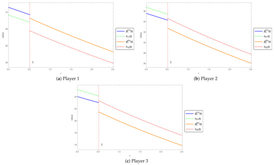
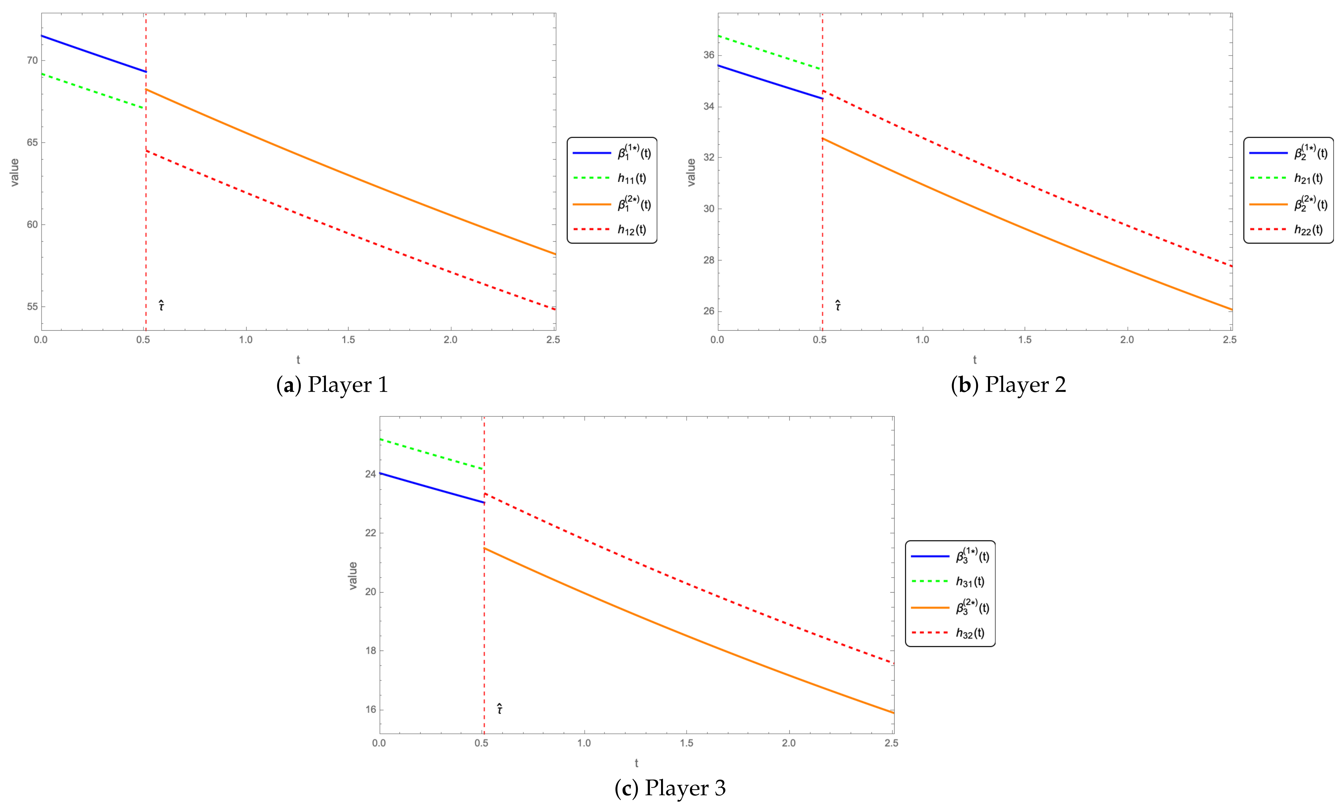
Panels (a)–(c) of Figure 1 plot the IDP payment rates and the corresponding discounted instantaneous payoff flows for players 1, 2, and 3, respectively. For player i, the solid blue curve represents the pre-switch IDP payment rate ${\beta }_i^{(1*)}\left(t\right)$, while the dashed green curve represents the pre-switch discounted instantaneous payoff flow $h_{i1}(e_i^{\left(1\right)}\left(t\right),P_1\left(t\right))$. After the realized switching time $\widehat{\tau }$, the solid orange curve represents the post-switch payment rate ${\beta }_i^{(2*)}\left(t\right)$, and the dashed red curve represents the post-switch discounted instantaneous payoff flow $h_{i2}(e_i^{\left(2\right)}\left(t\right),P_2\left(t\right))$.

Figure 1. IDP payment rates and discounted instantaneous payoff flows for the three players. The vertical dashed line marks the realized switching time $\widehat{\tau }=0.510522$. Before the switch, the curves correspond to ${\beta }_i^{(1*)}\left(t\right)$ and $h_{i1}(e_i^{\left(1\right)}\left(t\right),P_1\left(t\right))$; after the switch, they correspond to ${\beta }_i^{(2*)}\left(t\right)$ and $h_{i2}(e_i^{\left(2\right)}\left(t\right),P_2\left(t\right))$, $i=1,2,3$.

The figures show that the IDP payment rates change at the realized switching time. For all three players, both the payment rates and the instantaneous payoff flows decrease over time, reflecting discounting and the evolution of the pollution stock along the cooperative trajectory.

The comparison between ${\beta }_i^{(j*)}\left(t\right)$ and $h_{ij}\left(t\right)$ illustrates that the IDP is not simply a pointwise assignment of each player’s own instantaneous payoff flow. Instead, the payment rate is obtained from the change in the player’s continuation Shapley value. Hence, the IDP implements the Shapley allocation dynamically: at each time, the remaining unpaid payoff is consistent with the Shapley value of the corresponding continuation game. This is precisely the time-consistency requirement imposed by the imputation distribution procedure.

5. Threshold-Triggered Exponential Switch

We extend the baseline model by allowing the switching risk to become active only after the pollution stock reaches a threshold. This captures cases where policy or damages escalate only when pollution becomes sufficiently high, while the implementation still has a random delay.

Fix a pollution threshold $P_1>0$ and define the first hitting time

$$t_1:=inf\{t\ge 0:P\left(t\right)=P_1\}.$$

(18)

Switching cannot occur before the threshold is reached. After reaching $P_1$, switching occurs with a constant hazard $\lambda$:

$$\tau =t_1+X,X\sim \mathrm{Exp}\left(\lambda \right),\lambda >0.$$

(19)

The damage weight is

$$\gamma \left(t\right)=\left\{\begin{array}{cc}\hfill {\gamma }_1,\hfill & \hfill t<\tau ,\hfill \\ \hfill {\gamma }_2,\hfill & \hfill t\ge \tau .\hfill \end{array}\right.$$

where $k_i>0$ is the emission constraint of player i:

$$0\le e_i\left(t\right)\le k_i,i=1,\dots ,n,t\ge 0.$$

(20)

5.1. Post-Threshold Continuation Problem ($t\ge t_1$, Hazard $\lambda$ Active)

Once the threshold is reached, the model becomes the same constant-hazard switching environment as in Section 2 (now interpreted as a post-threshold subproblem). Therefore, the post-threshold continuation value at the threshold state is

$$e^{-r{t}_1}{V}_1^{\mathrm{th}}\left(P_1\right)=e^{-r{t}_1}(A_1+B_1{P}_1).$$

(21)

5.2. Pre-Threshold Subproblem on $[0,t_1]$ (Hazard 0, Fixed Endpoint $P\left(t_1\right)=P_1$)

Fix a candidate hitting time $t_1>0$. Since switching cannot occur before $t_1$, the planner solves a finite-horizon control problem with fixed endpoints:

$$\underset{{\left\{e_i\right\}}_{t\in [0,t_1]}}{max}{\int }_0^{t_1}{e}^{-rt}\left({\displaystyle \sum _{i=1}^n}\left(b_i{e}_i\left(t\right)-{\displaystyle \frac{1}{2}}{e}_i{\left(t\right)}^2\right)-n{\gamma }_{1}P\left(t\right)\right)dt,P\left(0\right)=P_0,P\left(t_1\right)=P_1,$$

(22)

subject to $\dot{P}={\sum }_i{e}_i-\alpha P$ and the constraint (20). This is a fixed-terminal-state problem with a free terminal time parameter $t_1$.

Let the current-value Hamiltonian be

$$H^{\mathrm{pre}}={\displaystyle \sum _{i=1}^n}\left(b_i{e}_i-{\displaystyle \frac{1}{2}}{e}_i^2\right)-n{\gamma }_{1}P+\mu \left({\displaystyle \sum _{i=1}^n}{e}_i-\alpha P\right).$$

The unconstrained FOC would give $e_i=b_i+\mu \left(t\right)$ and the costate equation

$$\dot{\mu }\left(t\right)=(r+\alpha )\mu \left(t\right)+n{\gamma }_1.$$

(23)

With the constraint, the implemented control is the projection

$$e_i^{\left(0\right)}\left(t\right)={\Pi }_{[0,k_i]}(b_i+\mu \left(t\right)),i=1,\dots ,n.$$

(24)

Writing $\kappa :=r+\alpha$ and $d:={\displaystyle \frac{n{\gamma }_1}{\kappa }}$, the costate has the explicit form

$$\mu \left(t\right)=c\left(t_1\right)e^{\kappa t}-d,$$

(25)

where the constant $c\left(t_1\right)$ is chosen so that the state trajectory under (24) satisfies the fixed endpoint $P\left(t_1\right)=P_1$.

5.3. Optimal Hitting Time $t_1^{*}$

For a given candidate $t_1>0$, let the pre-threshold value be

$$J_1\left(t_1\right):={\int }_0^{t_1}{e}^{-rt}\left[{\displaystyle \sum _{i=1}^n}\left(b_i{e}_i^{\left(0\right)}\left(t\right)-{\displaystyle \frac{1}{2}}{\left(e_i^{\left(0\right)}\left(t\right)\right)}^2\right)-n{\gamma }_1{P}_0\left(t\right)\right]dt,$$

where $P_0\left(t\right)$ is the solution of (1) under controls (24) with $P\left(0\right)=P_0$, $P\left(t_1\right)=P_1$.

The total value associated with $t_1$ is

$$W\left(t_1\right)=J_1\left(t_1\right)+e^{-r{t}_1}{V}_1^{\mathrm{th}}\left(P_1\right).$$

(26)

Hence, the optimal threshold-hitting time is

$$t_1^{*}\in arg\underset{t_1>0}{max}W\left(t_1\right).$$

In computations, we solve for $t_1^{*}$ by one-dimensional numerical maximization of $W\left(t_1\right)$. This direct approach is robust because the constraints can create kinks (at both 0 and $k_i$), so $W\left(t_1\right)$ is generally only piecewise smooth.

The pre-threshold current-value Hamiltonian at $t=t_1$ is

$$H^{\mathrm{pre}}\left(t_1\right)={\displaystyle \sum _{i=1}^n}\left(b_i{e}_i^{\left(0\right)}\left(t_1\right)-{\displaystyle \frac{1}{2}}{\left(e_i^{\left(0\right)}\left(t_1\right)\right)}^2\right)-n{\gamma }_1{P}_1+{\mu }_1\left({\displaystyle \sum _{i=1}^n}{e}_i^{\left(0\right)}\left(t_1\right)-\alpha P_1\right),$$

where ${\mu }_1:=\mu \left(t_1\right)$.

The standard free-terminal-time envelope identity with fixed terminal state $P\left(t_1\right)=P_1$ yields (see, e.g., Seierstad & Sydsæter, 1987)

$${\displaystyle \frac{d}{d{t}_1}}{J}_1\left(t_1\right)=e^{-r{t}_1}{H}^{\mathrm{pre}}\left(t_1\right).$$

(27)

Differentiating (26) and using (27), we obtain

$$W^{\prime }\left(t_1\right)=e^{-r{t}_1}\left(H^{\mathrm{pre}}\left(t_1\right)-r{V}_1^{\mathrm{th}}\left(P_1\right)\right).$$

(28)

Diagnostic Equation for $t_1^{*}$

On any smooth branch, a necessary condition for an interior maximizer is $W^{\prime }\left(t_1\right)=0$. By (28), this is equivalent to

$$g\left(t_1\right):=H^{\mathrm{pre}}\left(t_1\right)-r{V}_1^{\mathrm{th}}\left(P_1\right)=0.$$

(29)

If, in addition, the terminal control is interior for all players,

$$0<b_i+{\mu }_1<k_i,i=1,\dots ,n,$$

then $e_i^{\left(0\right)}\left(t_1\right)=b_i+{\mu }_1$ and the Hamiltonian simplifies to

$$H^{\mathrm{pre}}\left(t_1\right)={\displaystyle \frac{1}{2}}{S}_{b^2}+S_b{\mu }_1+{\displaystyle \frac{1}{2}}n{\mu }_1^2-n{\gamma }_1{P}_1-\alpha {\mu }_1{P}_1,$$

(30)

which gives the explicit interior-branch diagnostic equation

$${\displaystyle \frac{1}{2}}{S}_{b^2}+S_b{\mu }_1+{\displaystyle \frac{1}{2}}n{\mu }_1^2-n{\gamma }_1{P}_1-\alpha {\mu }_1{P}_1-r{V}_1^{\mathrm{th}}\left(P_1\right)=0.$$

5.4. Numerical Illustration

This subsection illustrates how the endogenous hitting time $t_1^{*}$ and the realized switching time $\tau =t_1^{*}+X$ shape the pollution path in the threshold-triggered model under the emission constraints (20).

For this threshold-triggered path illustration, we consider a five-player example with

$$\begin{array}{cc}& \hfill N=5,{\left(b_i\right)}_{i=1}^5=(12.0,11.2,10.7,10.1,9.6),\hfill \\ & \hfill r=0.05,\alpha =0.10,\lambda =0.30,{\gamma }_1=0.10,{\gamma }_2=0.30,\hfill \end{array}$$

and

$$P_0=0.20,P_1=2.00.$$

The emission caps are set uniformly as

$$(k_1,k_2,k_3,k_4,k_5)=(3.0,3.0,3.0,3.0,3.0).$$

These caps make the projection operator active in the numerical example. In the post-threshold pre-switch regime, the unconstrained emission vector

$$(4.222,3.422,2.922,2.322,1.822)$$

is projected to

$$(3.000,3.000,2.922,2.322,1.822).$$

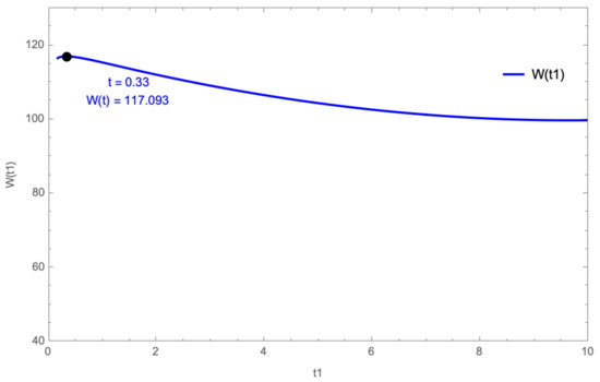
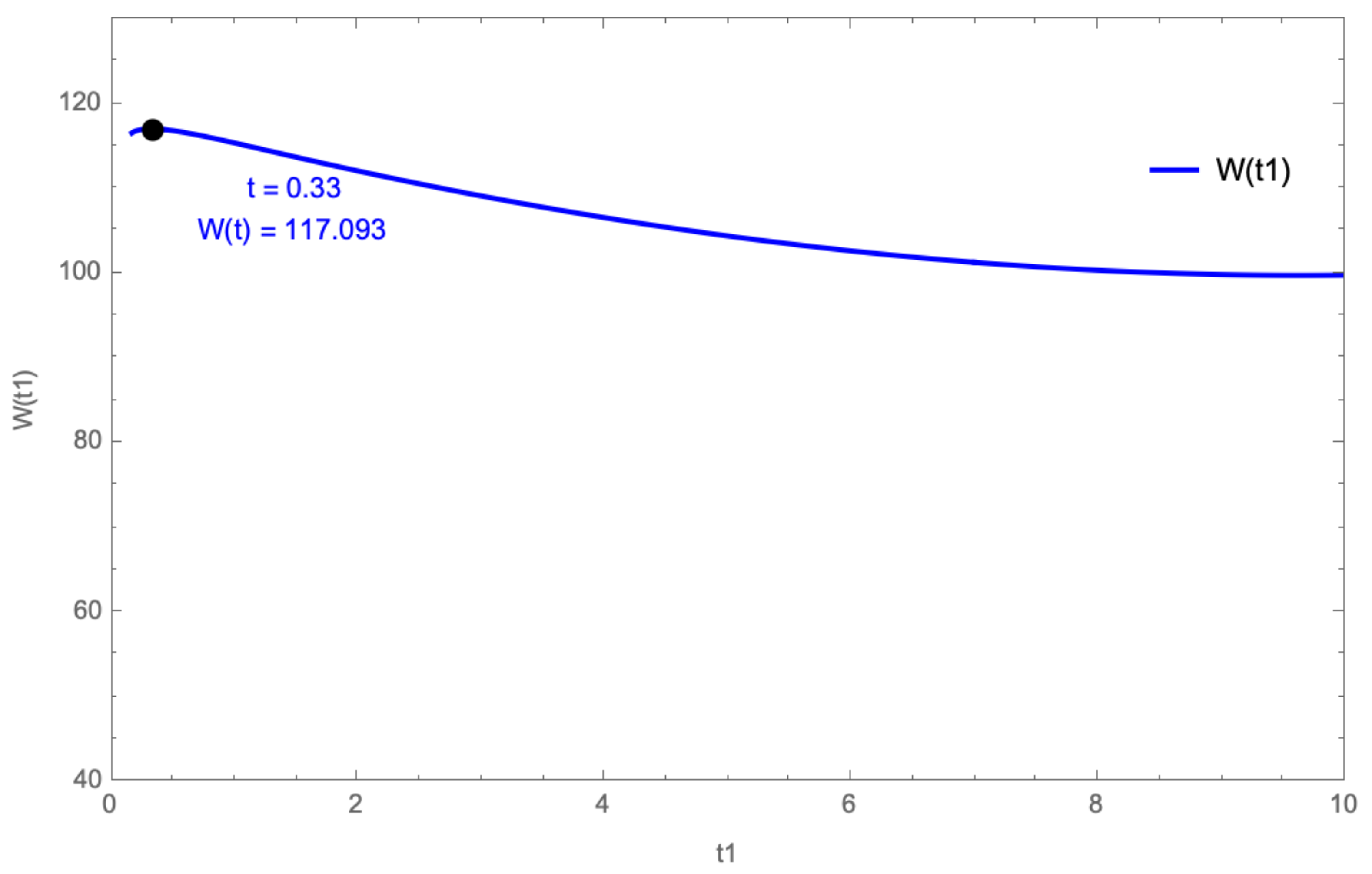
We maximize $W\left(t_1\right)$ numerically to obtain the optimal threshold-hitting time. For the above parameters, the maximization yields

$$t_1^{*}\approx 0.327792,W\left(t_1^{*}\right)\approx 117.093.$$

Figure 2 illustrates the one-dimensional maximization problem. The objective $W\left(t_1\right)$ reaches its maximum near $t_1^{*}$, after which the value gradually decreases as the threshold-hitting time is delayed.

Figure 2. The total value $W\left(t_1\right)$ under the uniform emission caps $k_i=3$. The marked point corresponds to the computed optimum $t_1^{*}\approx 0.327792$, with $W\left(t_1^{*}\right)\approx 117.093$.

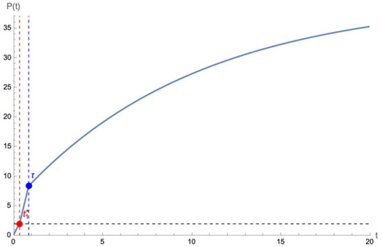
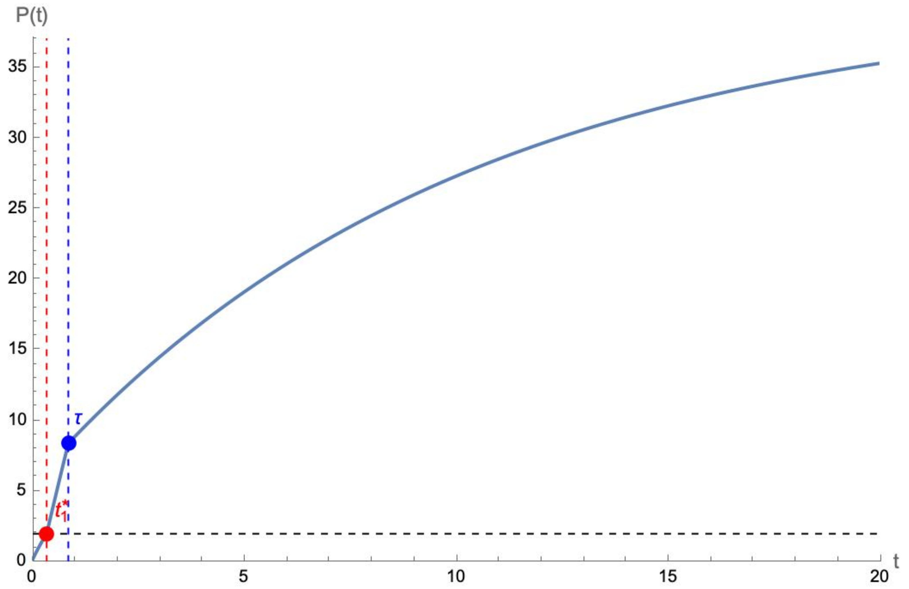
To generate the simulated pollution path in Figure 3, conditional on $t_1^{*}$, we draw one realization of $X\sim \mathrm{Exp}\left(\lambda \right)$. With the fixed random seed used in the numerical simulation, this gives

$$X\approx 0.510522,\tau =t_1^{*}+X\approx 0.838314.$$

Figure 3. Simulated pollution path $P\left(t\right)$ under the uniform emission caps $0\le e_i\left(t\right)\le 3$. The solid blue curve shows the simulated pollution path. The black dashed horizontal line denotes the threshold $P_1=2.00$, the red dashed vertical line marks the optimal hitting time $t_1^{*}\approx 0.327792$, and the blue dashed vertical line marks the realized switching time $\tau \approx 0.838314$. The red dot indicates the threshold-hitting point, and the blue dot indicates the pollution stock at the realized switching time.

On $[0,t_1^{*})$, the hazard is zero and the planner drives the stock to the fixed endpoint $P_1$. On $[t_1^{*},\tau )$, the hazard is active but the regime has not switched yet. At $t=\tau$, the damage weight jumps from ${\gamma }_1$ to ${\gamma }_2$, while the state $P\left(t\right)$ remains continuous.

6. Conclusions

This paper studies a pollution control differential game featuring a one-time increase in public damage weight at a random, exponentially distributed switching time. The model is solved using standard continuous-time dynamic programming, resulting in closed-form cooperative feedback policies for each regime in the baseline scenario. The characteristic function is constructed under pointwise emission caps and a conservative outsider benchmark. For the cooperative solution, a time-consistent imputation distribution procedure (IDP) is proposed to implement the Shapley allocation along the stochastic pollution path.

The numerical illustration shows how the characteristic function, the Shapley vector, and the corresponding IDP payment rule can be computed in practice. It also shows how active emission caps affect the constrained cooperative path and how the threshold-triggered mechanism links the switching risk to the pollution stock.

Finally, we extend the model to a threshold-triggered shifted-exponential specification, where switching risk activates only after the pollution stock reaches a threshold. The problem is separated into (i) a post-threshold continuation value solved via the HJB equation and (ii) a pre-threshold fixed-endpoint problem solved using the truncated maximum principle. The optimal hitting time $t_1^{*}$ is obtained by maximizing the one-dimensional objective $W\left(t_1\right)$, subject to the diagnostic condition $g\left(t_1\right)=0$ on smooth branches. The threshold and hazard parameters provide a tractable interpretation of ecological or regulatory regime changes.

References

- Basar, T., & Olsder, G. J. (1999). Dynamic noncooperative game theory (2nd ed.). SIAM. [Google Scholar] [CrossRef] [Scilit]
- Dockner, E. J., Jørgensen, S., Van Long, N., & Sorger, G. (2000). Differential games in economics and management science. Cambridge University Press. [Google Scholar] [CrossRef] [Scilit]
- Dockner, E. J., & Long, N. V. (1993). International pollution control: Cooperative versus noncooperative strategies. Journal of Environmental Economics and Management, 25, 13–29. [Google Scholar] [CrossRef] [Scilit]
- Fleming, W. H., & Soner, H. M. (2006). Controlled Markov processes and viscosity solutions (2nd ed.). Springer. [Google Scholar] [CrossRef] [Scilit]
- Kossioris, G., Plexousakis, M., Xepapadeas, A., de Zeeuw, A., & Mäler, K.-G. (2008). Feedback Nash equilibria for non-linear differential games in pollution control. Journal of Economic Dynamics and Control, 32, 1312–1331. [Google Scholar] [CrossRef] [Scilit]
- Kostyunin, S. Y., & Shevkoplyas, E. V. (2011). On simplification of integral payoff in differential games with random duration. Vestnik of St. Petersburg University. Series 10. Applied Mathematics. Informatics. Control Processes, 4, 47–56. Available online: https://www.mathnet.ru/eng/vspui57 (accessed on 24 May 2026).
- Lv, S. (2020). Two-player zero-sum stochastic differential games with regime switching. Automatica, 114, 108819. [Google Scholar] [CrossRef] [Scilit]
- Mao, X., & Yuan, C. (2006). Stochastic differential equations with Markovian switching. Imperial College Press. [Google Scholar] [CrossRef] [Scilit]
- Petrosjan, L. A. (2005). Cooperative differential games. In A. Haurie, S. Muto, L. A. Petrosjan, & T. E. S. Raghavan (Eds.), Advances in dynamic games: Applications to economics, finance, optimization, and stochastic control (pp. 183–200). Birkhäuser. [Google Scholar] [CrossRef] [Scilit]
- Petrosyan, L. A., & Danilov, N. N. (1979). Stability of solutions in non-zero sum differential games with transferable payoffs. Vestnik Leningradskogo Universiteta, 1, 52–79. (In Russian) [Google Scholar]
- Rubio, S. J., & Casino, B. (2002). A note on cooperative versus non-cooperative strategies in international pollution control. Resource and Energy Economics, 24, 251–261. [Google Scholar] [CrossRef] [Scilit]
- Seierstad, A., & Sydsæter, K. (1987). Optimal control theory with economic applications. North-Holland. [Google Scholar]
- Shapley, L. S. (1953). A value for n-person games. In H. W. Kuhn, & A. W. Tucker (Eds.), Contributions to the theory of games II (pp. 307–317). Princeton University Press. [Google Scholar] [CrossRef] [Scilit]
- Tur, A. V., & Gromova, E. V. (2020). On optimal control of pollution emissions: An example of the largest industrial enterprises of Irkutsk Oblast. Automation and Remote Control, 81, 548–565, (Original work published 2018). [Google Scholar] [CrossRef] [Scilit]
- von Neumann, J., & Morgenstern, O. (1953). Theory of games and economic behavior (3rd ed.). Princeton University Press. [Google Scholar]
- Yeung, D. W. K., & Petrosyan, L. A. (2006). Cooperative stochastic differential games. Springer. [Google Scholar] [CrossRef] [Scilit]
- Yin, G. G., & Zhu, C. (2010). Hybrid switching diffusions: Properties and applications. Springer. [Google Scholar] [CrossRef] [Scilit]
- Zaccour, G. (2003). Computation of characteristic function values for linear-state differential games. Journal of Optimization Theory and Applications, 117, 183–194. [Google Scholar] [CrossRef] [Scilit]
- Zaremba, A. P. (2022). Cooperative differential games with the utility function switched at a random time moment. Matematicheskaya Teoriya Igr i Prilozheniya, 14, 31–50. [Google Scholar] [CrossRef] [Scilit]
Disclaimer/Publisher’s Note: The statements, opinions and data contained in all publications are solely those of the individual author(s) and contributor(s) and not of MDPI and/or the editor(s). MDPI and/or the editor(s) disclaim responsibility for any injury to people or property resulting from any ideas, methods, instructions or products referred to in the content. |
© 2026 by the authors. Licensee MDPI, Basel, Switzerland. This article is an open access article distributed under the terms and conditions of the Creative Commons Attribution (CC BY) license.