A Provable Semi-Infinite Programming Approach for Solving Constrained Dynamic Games

Abstract

Many engineering problems must account for the non-cooperative decisions and actions of multiple players. These problems can be modeled within a game-theoretic framework. The approach herein is to model such problems as mathematical games, convert them to semi-infinite programs, and utilize a semi-infinite program solver whose output is provably an $ϵ$-optimal Nash equilibrium. The approach is successfully benchmarked on two low-dimensional problems. Two types of higher-dimensional linear quadratic dynamic games are then investigated: ones where each player’s problem is convex and ones where at least one player’s problem is nonconvex. Within each type, variations based on information structure, control constraints, number of players, and semi-infinite objective are considered. The algorithm is tested with different internal solvers, and it successfully solves all test problems using MATLAB’s fmincon. The numerical solutions approximate analytical solutions (when they are known) within approximately one percent. For a three-player game with input saturation constraints, hundreds of variables, and no analytical solution, the computational time is approximately five minutes.

1. Introduction

Game theory has numerous applications in wildlife management (Engwerda, 2018), power systems (Mylvaganam & Astolfi, 2015), traffic control (Colombo et al., 2025), evolutionary biology (Taylor & Jonker, 1978) and more (Guo et al., 2013; Huang & Zhao, 2021). A simple, quintessential example is that of a children’s game of tag—formally called pursuit and evasion—in which the pursuer minimizes its distance to a given evader and evaders maximize their distance to the pursuer. The players make decisions and take actions to optimize their respective outcomes understanding that others are doing the same. This is a non-cooperative game. The game is dynamic because the players’ states evolve according to differential or difference equations. Militaristic variations of this problem are pervasive and described in the early work of Isaacs (1965). Other notable examples from engineering/control, mathematical theories, and algorithms have been presented in the books by Bryson and Ho (1975) and Başar and Olsder (1999).

Because games involve the simultaneous solution of multiple optimization problems, standard linear, convex, and nonlinear programming solvers cannot directly solve games, though they can still indirectly be used by embedding optimality conditions as constraints within the solvers. For this reason, myriad numerical methods have been developed. Chenchene et al. (2025) proposed using agents to sample the solution space for the global Nash equilibrium with termination based on agent consensus. Another method by Garagic and Cruz (2003) uses fuzzy set theory to solve static Nash games by dividing the problem into three phases: fuzzification, inference, and defuzzification. In the work by Guo et al. (2013), semi-tensor products are used to find Nash equilibria for static games. A dynamic pursuer–evader game is solved by Pontani and Conway (2009) using a genetic algorithm to formulate an initial guess for a semi-direct collocation with nonlinear programming algorithm. A special subset of pursuer–evader games includes minimax games, where one player tries to minimize the same objective that the other player is trying to maximize. A method used to solve minimax games in machine learning is a gradient descent–ascent algorithm (Lin et al., 2020; Nouiehed et al., 2019). This method performs a step of gradient descent for one player and a step of gradient ascent for the other player for every iteration.

Embedding optimality conditions, specifically the Karush–Kuhn–Tucker (KKT) conditions (Berkovitz, 2002), of some or all players as constraints presents three challenges. First, KKT conditions have a constraint qualification (commonly linear independence or Mangasarian–Fromovitz) that is difficult to verify a priori. When the qualification is violated, the conditions are not solvable. Simple finite-dimensional examples are Example 5.2 of Berkovitz (2002) and Example 3.7 of Harris and Rose (2023). A practical optimal control problem that fails the constraint qualification is presented in Problem 5.10 of Harris and Rose (2023). If any player has such a problem in the Nash setting, this “KKT embedding” approach will fail. Second, when inequality constraints are present, the linear independence constraint qualification is trivially violated because gradients of the active inequality constraints and complementary slackness conditions are linearly dependent. Third, KKT conditions are only necessary conditions for nonconvex programs and may lead to spurious solutions. For these reasons, this paper pursues a “direct” approach that does not leverage KKT conditions.

In this paper, Nash games are transformed into semi-infinite programs (SIPs) so that an entirely different set of algorithms are applicable. SIPs are mathematical programs with a finite number of decision variables and an infinite number of constraints. The infinite constraints are typically formulated as inequalities with one or more variables belonging to an infinite set. These programs are commonly used in engineering problems for robustness (Ben-Tal & Nemirovski, 1999), the design of control Lyapunov functions (Tang & Daoutidis, 2023), worst-case control design (Polak & Stimler, 1988), design centering (Stein, 2006), set covering problems (Krieg et al., 2022), and more (Hettich & Kortanek, 1993; López & Still, 2007). There are many numerical approaches to solving SIPs based on interval methods (Bhattacharjee et al., 2005a), branch-and-bound (Bhattacharjee et al., 2005b), and the use of various lower and upper bounding problems (Cerulli et al., 2022; Feng et al., 2020; Floudas & Stein, 2008; Mitsos, 2011). The algorithmic literature is immense with approaches based on integral function transformation (Ling et al., 2006), proximal bundles (Pang & Wu, 2022), relaxations (Mitsos et al., 2008), spectral factorization (Hayashi & Wu, 2010), and more having been proposed (Djelassi et al., 2021). MATLAB has a built-in SIP solver fseminf (The MathWorks Inc., 2024). It does not generate a provably optimal point, and dimensional limitations make it inapplicable to the dynamic games of interest in this paper. Nonetheless, it is tested on the benchmark problems described in Section 2 for completeness.

With the goal of solving dynamic Nash games as SIPs, the primary algorithm of interest is one by Mitsos (2011). It uses commercially available off-the-shelf solvers to solve so-called lower-bounding, lower-level, and upper-bounding problems. The commercially available solver is henceforth referred to as the “internal solver”. By cycling through these problems, the algorithm converges finitely to a provably $ϵ$-optimal point—for both the SIP and the Nash game. Assumptions for convergence are mild and trivially satisfied by the construction of the SIP. Upcoming results explore the use of both global (Gurobi (Gurobi Optimization, LLC, 2024)) and local (MATLAB’s fmincon (The MathWorks Inc., 2024)) internal solvers. There is a natural trade-off between proving global optimality of the SIP solution and computation time. The ease of implementation, flexibility in choosing the internal solver, and convergence guarantees make the algorithm a promising one for solving challenging, constrained Nash games in SIP form.

The primary contributions of the paper are: (1) the transformation of a Nash game into a numerically solvable SIP; (2) the identification of a suitable SIP solver that generates a provably $ϵ$-optimal Nash solution; and (3) successful demonstration on benchmark problems and larger-scale dynamic games. An outline of the paper is as follows. Section 2 introduces Nash games, transformation to SIP form, and results on simple benchmark problems. In Section 3, larger-scale problems are solved. These have hundreds of decision variables and include a series of convex linear–quadratic games with and without control constraints for two and three players. Numerical solutions are compared with both open-loop and closed-loop theoretical solutions when possible. Nonconvex pursuer–evader games in both Nash and sequential forms are considered in Section 4. This paper is concluded in Section 5.

2. Approach and Benchmark Results

In this section, the problems of interest are two-player Nash games. The decision variables for the players are $x_1\in {\mathbb{R}}^{n_1}$ and $x_2\in {\mathbb{R}}^{n_2}$, their constraint sets are $X_1\subset {\mathbb{R}}^{n_1}$ and $X_2\subset {\mathbb{R}}^{n_2}$, and their objective functions are $f_1:X_1\times X_2\to \mathbb{R}$ and $f_2:X_1\times X_2\to \mathbb{R}$. Each player’s goal is to minimize its objective function by selecting an element from its constraint set. In a typical problem, the constraint sets are generated by equalities and inequalities, and they contain infinitely many elements. Because the objective functions depend on all players’ decisions, the Nash game is not solvable as a single standard optimization problem.

Definition 1.

A point $(x_1,x_2)\in X_1\times X_2$ is a locally optimal Nash solution (equilibrium) if there exist neighborhoods $N\left(x_1\right)\subset X_1$ and $N\left(x_2\right)\subset X_2$ of $x_1$ and $x_2$, respectively, such that

$$\begin{array}{c}\hfill \forall \gamma \in N\left(x_1\right),f_1(x_1,x_2)-f_1(\gamma ,x_2)\le 0,\end{array}$$

(1a)

$$\begin{array}{c}\hfill \forall \zeta \in N\left(x_2\right),f_2(x_1,x_2)-f_2(x_1,\zeta )\le 0.\end{array}$$

(1b)

If $N\left(x_1\right)=X_1$ and $N\left(x_2\right)=X_2$, then $(x_1,x_2)$ is a globally optimal Nash solution.

Recognizing that each player is solving an optimization problem with the other player’s decision fixed leads to simple necessary and sufficient conditions for local solutions of unconstrained, differentiable games.

Lemma 1.

Let $X_1$ and $X_2$ be open. Let $f_1$ and $f_2$ be twice continuously differentiable. If $(x_1,x_2)$ is a Nash solution, then

$${\displaystyle \frac{\partial }{\partial x_i}}{f}_i(x_1,x_2)=0,{\displaystyle \frac{{\partial }^2}{\partial x_i^2}}{f}_i(x_1,x_2)\ge 0,i=1,2.$$

(2)

Also, if

$${\displaystyle \frac{\partial }{\partial x_i}}{f}_i(x_1,x_2)=0,{\displaystyle \frac{{\partial }^2}{\partial x_i^2}}{f}_i(x_1,x_2)>0,i=1,2,$$

(3)

then $(x_1,x_2)$ is a locally optimal Nash solution.

The first-order conditions provide a means of generating candidate equilibria by solving a system of algebraic equations. This idea can be extended to problems with constraints; however, there are challenges with this KKT approach as described in the Introduction. A related solution concept is that of $ϵ$-optimality.

Definition 2.

For a given $ϵ>0$, a point $(x_1,x_2)\in X_1\times X_2$ is a locally ϵ-optimal Nash solution if there exist neighborhoods $N\left(x_1\right)\subset X_1$ and $N\left(x_2\right)\subset X_2$ of $x_1$ and $x_2$, respectively, such that

$$\begin{array}{c}\hfill \forall \gamma \in N\left(x_1\right),f_1(x_1,x_2)-f_1(\gamma ,x_2)-ϵ\le 0,\end{array}$$

(4a)

$$\begin{array}{c}\hfill \forall \zeta \in N\left(x_2\right),f_2(x_1,x_2)-f_2(x_1,\zeta )-ϵ\le 0.\end{array}$$

(4b)

If $N\left(x_1\right)=X_1$ and $N\left(x_2\right)=X_2$, then $(x_1,x_2)$ is a globally ϵ-optimal Nash solution.

Conceptually, an $ϵ$-optimal point produces an objective value that is at most $ϵ$ different than an optimal point. For a given $ϵ>0$, the $ϵ$-optimality inequalities in Equation (4) are now embedded as constraints in the following SIP:

$$\begin{array}{cc}\hfill \underset{x_1,x_2}{min}& F(x_1,x_2)\hfill \end{array}$$

(5a)

$$\begin{array}{cc}\hfill \mathrm{subject}\mathrm{to}& f_1(x_1,x_2)-f_1(\gamma ,x_2)-ϵ\le 0,\forall \gamma \in X_1\hfill \end{array}$$

(5b)

$$\begin{array}{cc}\hfill & f_2(x_1,x_2)-f_2(x_1,\zeta )-ϵ\le 0,\forall \zeta \in X_2\hfill \end{array}$$

(5c)

$$\begin{array}{cc}\hfill & x_1\in X_1,x_2\in X_2\hfill \end{array}$$

(5d)

The optimization variables are $x_1$ and $x_2$. Provided either $X_1$ or $X_2$ has infinitely many elements, there are infinite constraints. Variables $\gamma$ and $\zeta$ are referred to as the semi-infinite variables. It is obvious that any SIP solution (feasible, local, or global) produces a globally $ϵ$-optimal Nash solution. As such, the choice of F is not theoretically important. In practice, however, F can have a regularizing effect on the problem that can accelerate solve times. When the $f_i$ are convex, obvious choices for F are $F=f_1$, $F=f_2$, and $F={\displaystyle \frac{1}{2}}{f}_1+{\displaystyle \frac{1}{2}}{f}_2$. When the $f_i$ are nonconvex, one can choose $F={\parallel x_1\parallel }_2^2+{\parallel x_2\parallel }_2^2$. These choices are explored in our numerical examples. Ultimately, the choice is problem dependent and up to the engineer.

The SIP in standard form is given below:

$$\begin{array}{cc}\hfill \underset{x}{min}& F\left(x\right)\hfill \end{array}$$

(6a)

$$\begin{array}{cc}\hfill \mathrm{subject}\mathrm{to}& g(x,y)\le 0,\forall y\in Y\hfill \end{array}$$

(6b)

$$\begin{array}{cc}\hfill & x\in X\hfill \end{array}$$

(6c)

The finite variable x corresponds to the player choices ${[x_1^T,x_2^T]}^T$ in Equation (5). The infinite variable y is ${[{\gamma }^T,{\zeta }^T]}^T$. Both belong to the infinite set $X=Y=X_1\times X_2$. The inequality $g(x,y)\le 0$ corresponds to the inequalities in Equations (5b) and (5c). The framework just described trivially generalizes to games with three or more players.

To solve the SIP, the algorithm by Mitsos (2011) is selected because it (1) generates an $ϵ$-optimal solution to the SIP (and hence the Nash game), (2) leverages commercially available solvers, and (3) has mild assumptions for finite convergence. Assumptions include continuity of functions F and g and compactness of X and Y. The final assumption is existence of a SIP-Slater point—a point x for which $g(x,y)<0$ for all $y\in Y$. By construction, the Nash equilibrium serves as this point because g is bounded above by $-ϵ$ at the Nash equilibrium.

The algorithm is described informally in words here. A formalized step-by-step description is given in Algorithm 1 on the next page. There are four subproblems solved in the algorithm: the lower-bounding problem, the lower-level problem based on the results from the lower-bounding problem, the upper-bounding problem, and finally the lower-level problem based on the results from the upper-bounding problem. The sets $Y_L$ and $Y_U$ are finite subsets of Y. Their initializations $Y_{L,0}$ and $Y_{U,0}$ are arbitrary and are subsequently populated by the algorithm. The lower-bounding problem form is nearly identical to Equation (6) with the only change being that Y is replaced with the finite set $Y_L$. The results from the lower-bounding problem are denoted $\overline{x}$. The lower-level problem is then defined as ${max}_{y\in Y}g(\overline{x},y)$. The results from this lower-level problem are added to $Y_L$. The form of the upper-bounding problem is also similar to Equation (6) with two changes: the infinite set Y is replaced with the finite set $Y_U$ and $g(x,y)\le -{ϵ}_g$. The results from the upper-bounding problem are denoted $\overline{x}$. The lower-level problem is then solved again and the results are added to $Y_U$. The parameter r is a scalar greater than one and is used to decrease the value of ${ϵ}_g$. The bounding values $f_L$ and $f_U$ are the values from the objective functions solved in the lower- and upper-bounding problems. To end the algorithm, a tolerance $ϵ$ is used. Initial guesses to the internal solver are required when using MATLAB’s fmincon but not when using Gurobi. In all subsequent problems, ${ϵ}_g$ is initialized at 0.8, $r=1.5$, and $ϵ=0.001$. A discussion and numerical demonstration of the effects of these parameters is given by Mitsos (2011).

Algorithm 1 Algorithm to solve SIP.

Input:    Finite subsets $Y_{L,0}\subset Y$ and $Y_{U,0}\subset Y$    Threshold values ${ϵ}_g>0$ and $ϵ>0$    Update rate $r>0$ Output:    SIP solution, $x^{*}$ Begin    Set fL = −∞, fU = ∞, YL = YL,0, YU = YU,0.    While $|f_U-f_L|>ϵ$      Do        Solve the lower-bounding problem, set $\overline{x}$ to the solution.        Solve the lower-level problem.        If the lower-level problem objective value is non-positive         $f_U=f_L$ and $x^{*}=\overline{x}$.        End        Add the lower-level problem solution to $Y_L$.        Solve the upper-bounding problem, set the solution equal to $f_{dum}$.        If feasible         Set $\overline{x}$ to the solution.         Solve the lower-level problem.         If the lower-level problem objective value is non-positive          If fdum ≤ fU           fU = fL $\mathrm{and}$ x* = $\overline{x}$          End          ϵg = ϵg/r.         Else           Add lower-level problem solution to YU.         End        Else          ϵg = ϵg/r.        End      End    End End

2.1. Benchmark Problems and Results

This subsection presents two benchmark problems: the “location game” and the “heat transfer game”. After describing the problem, its solution is obtained via Lemma 1 for comparative purposes with the SIP solutions. In each game, the decision variables are scalars, and the SIP objective is chosen to be $F=x_1^2+x_2^2$ since the $f_i$ are nonconvex. The computer used to solve each of these benchmark problems will be referred to as Computer One: 64-bit 12th Gen Intel(R) Core(TM) i9-12900H at 2.50 GHz running Windows 11 and Gurobi 11.0.0.

2.1.1. Location Game

Each player in the location game aims to be near the origin while also being far from the other player (Ratliff et al., 2013). The locations of the players on the number line are $x_1$ and $x_2$. Objective functions are specified below. The first terms drive each player to the origin; the second terms drive the players apart. The second player is penalized slightly more for being close to the first player:

$$\begin{array}{cc}\hfill f_1(x_1,x_2)& =-cos\left(x_1\right)+1.00cos(x_1-x_2)\hfill \end{array}$$

(7)

$$\begin{array}{cc}\hfill f_2(x_1,x_2)& =-cos\left(x_2\right)+1.05cos(x_2-x_1)\hfill \end{array}$$

(8)

To avoid trigonometric non-uniqueness, we only investigate equilibria in the range $(-\pi ,\pi )$. Lemma 1 applies, and the derivatives are

$$\begin{array}{cc}\hfill {\displaystyle \frac{\partial }{\partial x_1}}{f}_1(x_1,x_2)& =sin\left(x_1\right)-1.00sin(x_1-x_2),\hfill \end{array}$$

(9)

$$\begin{array}{cc}\hfill {\displaystyle \frac{\partial }{\partial x_2}}{f}_2(x_1,x_2)& =sin\left(x_2\right)-1.05sin(x_2-x_1),\hfill \end{array}$$

(10)

$$\begin{array}{cc}\hfill {\displaystyle \frac{{\partial }^2}{\partial x_1^2}}{f}_1(x_1,x_2)& =cos\left(x_1\right)-1.00cos(x_1-x_2),\hfill \end{array}$$

(11)

$$\begin{array}{cc}\hfill {\displaystyle \frac{{\partial }^2}{\partial x_2^2}}{f}_2(x_1,x_2)& =cos\left(x_2\right)-1.05cos(x_2-x_1).\hfill \end{array}$$

(12)

Setting the first-order conditions to zero, using Newton’s method to solve the nonlinear system, and checking for positive second derivatives yields two candidates, $(x_1,x_2)\approx (\pm 1.0181,\mp 1.1054)$, which are Nash equilibria.

The location game is now solved as an SIP, described in Equation (5). The initial finite set is populated with 1000 uniformly distributed random numbers in the range $(-\pi ,\pi )$. Table 1 shows the results for different internal solvers and initial guesses (when required). Results obtained from MATLAB’s SIP solver fseminf are shown for completeness. The algorithm consistently approximates the known equilibria using both fmincon and Gurobi. fseminf performs inconsistently based on the initial guess.

Table 1. Numerical SIP results for the location game.

	Initial Guess	Solution	CPU Time (s)	Iter
fmincon	(2, −2)	(1.0169, −1.1053)	0.585	1
	(−2, 2)	(−1.0173, 1.1058)	0.446	1
	(0, −2)	(1.0164, −1.1057)	2.444	2
	(0, 2)	(−1.0171, 1.1043)	3.759	1
	(0, 0)	(−1.0186, 1.1040)	1.019	1
	(2, 2)	(1.0167, −1.1046)	3.923	2
	(−2, −2)	(−1.0209, 1.1016)	4.267	2
Gurobi	N/A	(1.0177, −1.1023)	0.7442	1
fseminf	(2, −2)	(−1.0189, 1.1038)	0.029	64
	(−2, 2)	(1.0170, −1.1059)	0.029	64
	(0, −2)	(1.0166, −1.1061)	0.007	12
	(0, 2)	(−1.0166, 1.1062)	0.007	11
	(0, 0)	(4.362, −4.362)	0.010	12
	(2, 2)	(0.0844, −0.0339)	0.005	3
	(−2, −2)	(−0.1056, 0.0138)	0.005	3

2.1.2. Heat Transfer Game

The heat transfer game represents two players in adjoining rooms of a building (Ratliff et al., 2016). The players try to maintain the temperature at a set point in thermodynamic equilibrium. The temperatures chosen by the players are $x_1$ and $x_2$. Objective functions are specified below. The first term in their objectives represents the energy cost at equilibrium; the second term is a cross-term used to model heat transfer effects (or thermodynamic coupling between the rooms).

$$\begin{array}{cc}\hfill f_1(x_1,x_2)& =0.5x_1^2-x_1{x}_2\hfill \end{array}$$

(13)

$$\begin{array}{cc}\hfill f_2(x_1,x_2)& =0.5x_2^2-x_1{x}_2\hfill \end{array}$$

(14)

There are no restrictions on the possible temperatures. Lemma 1 applies, and the derivatives are

$$\begin{array}{cc}\hfill {\displaystyle \frac{\partial }{\partial x_1}}{f}_1(x_1,x_2)& =x_1-x_2,{\displaystyle \frac{{\partial }^2}{\partial x_1^2}}{f}_1(x_1,x_2)=1,\hfill \end{array}$$

(15)

$$\begin{array}{cc}\hfill {\displaystyle \frac{\partial }{\partial x_2}}{f}_2(x_1,x_2)& =x_2-x_1,{\displaystyle \frac{{\partial }^2}{\partial x_2^2}}{f}_2(x_1,x_2)=1.\hfill \end{array}$$

(16)

Setting the first-order conditions to zero yields a continuum of candidates along the line $x_1=x_2$. The second-order derivatives are always positive; hence, any point on the line is a Nash equilibrium.

The heat transfer game is now solved as a SIP described in Equation (5). The initial finite set is populated with 1000 uniformly distributed random numbers in the range $(-100,100)$. Table 2 shows results for different internal solvers and initial guesses (when required). The algorithm consistently approximates known equilibria, most of which are near the origin because $F=x_1^2+x_2^2$. fseminf also approximates equilibria along the line $x_1=x_2$, but solutions vary based on the initial guess.

Table 2. Numerical SIP results for the heat transfer game.

	Initial Guess	Solution	CPU Time (s)	Iter
fmincon	(1, 1)	(0.252, 0.252)	0.831	1
	(0, 0)	${10}^{-10}\times$ (0.391, −0.360)	0.562	1
	(−1, −1)	(−0.6618, −0.6618)	0.726	1
	(−1, 1)	${10}^{-10}\times$ (0.331, 0.691)	0.796	1
	(1, −1)	${10}^{-10}\times$ (−0.604, −0.046)	0.759	1
Gurobi	N/A	(0, 0)	0.241	1
fseminf	(1, 1)	(0.2929, 0.2929)	0.007	3
	(0, 0)	(0, 0)	0.013	2
	(−1, −1)	(−0.2927, −0.2929)	0.064	2
	(−1, 1)	(−0.1335, −0.1347)	0.083	26
	(1, −1)	(0.5331, 0.5277)	0.087	35

2.2. Summary of Benchmark Results

The benchmark results show that the proposed approach can successfully solve Nash games, and that the algorithm is successful using either the local or global internal solver. These benchmark games have only two scalar decision variables. For such small problems, differences in CPU time between the local and global solver are insignificant. In fact, there are instances where the global solver is faster. The commercially available fseminf has no convergence guarantees and solution quality is worse than with the proposed approach. CPU times, however, are faster. Upcoming sections focus on dynamic Nash games with hundreds of variables and use the local fmincon for speed. fseminf has dimensional limitations and cannot be used on such large problems.

3. Convex Linear Quadratic Dynamic Games

3.1. Two Player

A discrete-time linear quadratic dynamic game with two players is now presented, solved analytically, and then solved numerically using the SIP formulation. The players’ objectives $f_i$ are convex, and SIP solutions are computed with different choices of F: $F=0$ and $F=\frac{1}{2}{f}_1+\frac{1}{2}{f}_2$. Finally, a variation of the dynamic game is presented in which the control magnitudes are constrained. The authors are unaware of any analytical solution to this problem, so only SIP solutions are presented. A key advantage of the SIP approach is the ability to solve such constrained problems while leveraging off-the-shelf solvers. The computer used to solve all problems in this section is Computer Two: 64-bit Intel Xeon(R) W-2245 at 3.90 GHz running Ubuntu 20.04.6.

The first player’s control at time index k is $u_{1,k}$. The second player’s control is $u_{2,k}$. Starting from a fixed initial condition $x_0$, they drive the following linear discrete-time system:

$$x_{k+1}=A{x}_k+B_1{u}_{1,k}+B_2{u}_{2,k},k=0,\dots ,N-1$$

(17)

The players have the following quadratic objectives. Throughout the paper, S’s are positive semidefinite, Q’s are positive semidefinite, and R’s are positive definite:

$$\begin{array}{cc}\hfill & f_1(u_1,u_2)=\frac{1}{2}{x}_N^T{S}_{1,N}{x}_N+\frac{1}{2}{\displaystyle \sum _{k=0}^{N-1}}{x}_k^T{Q}_1{x}_k+u_{1,k}^T{R}_{11}{u}_{1,k}+u_{2,k}^T{R}_{12}{u}_{2,k}\hfill \end{array}$$

(18)

$$\begin{array}{cc}\hfill & f_2(u_1,u_2)=\frac{1}{2}{x}_N^T{S}_{2,N}{x}_N+\frac{1}{2}{\displaystyle \sum _{k=0}^{N-1}}{x}_k^T{Q}_2{x}_k+u_{1,k}^T{R}_{21}{u}_{1,k}+u_{2,k}^T{R}_{22}{u}_{2,k}\hfill \end{array}$$

(19)

Theoretical solutions can be derived for each player using standard optimal control techniques, such as the sweep method used by Bryson and Ho (1975). The Hamiltonians, transversality, stationarity, and costate equations are the same for both the open- and closed-loop information structure solutions.

• Player One Optimality Conditions

$$\begin{array}{c}\hfill \begin{array}{cc}\hfill & H_1^k={\displaystyle \frac{1}{2}}\left(x_k^T{Q}_1{x}_k+u_{1,k}^T{R}_{1,1}{u}_{1,k}+u_{2,k}^T{R}_{1,2}{u}_{2,k}\right)\hfill \\ \hfill & +{\lambda }_{1,k+1}^T\left(A{x}_k+B_1{u}_{1,k}+B_2{u}_{2,k}\right)\hfill \end{array}\end{array}$$

(20)

$$\begin{array}{cc}\hfill & {\lambda }_{1,N}=S_{1,N}{x}_N\hfill \end{array}$$

(21)

$$\begin{array}{cc}\hfill & u_{1,k}=-R_{1,1}^{-1}{B}_1^T{\lambda }_{1,k+1}\hfill \end{array}$$

(22)

$$\begin{array}{cc}\hfill & {\lambda }_{1,k}=Q_1{x}_k+A^T{\lambda }_{1,k+1}+{\displaystyle \frac{\partial u_{2,k}}{\partial x_k}}{R}_{1,2}{u}_{2,k}+{\displaystyle \frac{\partial u_{2,k}}{\partial x_k}}{B}_2^T{\lambda }_{1,k+1}\hfill \end{array}$$

(23)

• Player Two Optimality Conditions

$$\begin{array}{c}\hfill \begin{array}{cc}\hfill & H_2^k={\displaystyle \frac{1}{2}}\left(x_k^T{Q}_2{x}_k+u_{1,k}^T{R}_{2,1}{u}_{1,k}+u_{2,k}^T{R}_{2,2}{u}_{2,k}\right)\hfill \\ \hfill & +{\lambda }_{2,k+1}^T\left(A{x}_k+B_1{u}_{1,k}+B_2{u}_{2,k}\right)\hfill \end{array}\end{array}$$

(24)

$$\begin{array}{cc}\hfill & {\lambda }_{2,N}=S_{2,N}{x}_N\hfill \end{array}$$

(25)

$$\begin{array}{cc}\hfill & u_{2,k}=-R_{2,2}^{-1}{B}_2^T{\lambda }_{2,k+1}\hfill \end{array}$$

(26)

$$\begin{array}{cc}\hfill & {\lambda }_{2,k}=Q_2{x}_k+A^T{\lambda }_{2,k+1}+{\displaystyle \frac{\partial u_{1,k}}{\partial x_k}}{R}_{2,1}{u}_{1,k}+{\displaystyle \frac{\partial u_{1,k}}{\partial x_k}}{B}_1^T{\lambda }_{2,k+1}\hfill \end{array}$$

(27)

The next step is to use the sweep method by inserting the sweep assumption into the stationarity equations:

$$\begin{array}{cc}\hfill & {\lambda }_{1,k+1}=S_{1,k+1}{x}_{k+1}\to u_{1,k}=-R_{1,1}^{-1}{B}_1^T{S}_{1,k+1}{x}_{k+1}\hfill \end{array}$$

(28)

$$\begin{array}{cc}\hfill & {\lambda }_{2,k+1}=S_{2,k+1}{x}_{k+1}\to u_{2,k}=-R_{2,2}^{-1}{B}_2^T{S}_{2,k+1}{x}_{k+1}\hfill \end{array}$$

(29)

These stationarity equations are then substituted into the state equation, and after simplifying, an equation for the future states is formed that is dependent on the current states:

$$\begin{array}{cc}\hfill x_{k+1}& =\underset{{\tilde{A}}_{k+1}}{\underbrace{{\left(I+B_1{R}_{1,1}^{-1}{B}_1^T{S}_{1,k+1}+B_2{R}_{2,2}^{-1}{B}_2^T{S}_{2,k+1}\right)}^{-1}A}}{x}_k={\tilde{A}}_{k+1}{x}_k\hfill \end{array}$$

(30)

The state equation is then substituted into the stationarity equations:

$$\begin{array}{cc}\hfill & u_{1,k}=-\underset{K_{1,k}}{\underbrace{R_{1,1}^{-1}{B}_1^T{S}_{1,k+1}{\tilde{A}}_{k+1}}}{x}_k=-K_{1,k}{x}_k\hfill \end{array}$$

(31)

$$\begin{array}{cc}\hfill & u_{2,k}=-\underset{K_{2,k}}{\underbrace{R_{2,2}^{-1}{B}_2^T{S}_{2,k+1}{\tilde{A}}_{k+1}}}{x}_k=-K_{2,k}{x}_k\hfill \end{array}$$

(32)

3.1.1. Closed-Loop Information Structure

To derive solutions with a closed-loop information structure, it is assumed that the partial derivative terms in the costate equations are nonzero and can be found by taking the partial derivative of the stationarity equations:

$$\begin{array}{cc}\hfill & {\displaystyle \frac{\partial u_{1,k}}{\partial x_k}}=-K_{1,k}^T\hfill \end{array}$$

(33)

$$\begin{array}{cc}\hfill & {\displaystyle \frac{\partial u_{2,k}}{\partial x_k}}=-K_{2,k}^T\hfill \end{array}$$

(34)

The partial derivative, stationarity, and sweep assumption are then substituted into the costate equation to get a recursive formula for $S_{1,k}$:

$$\begin{array}{c}\hfill \begin{array}{cc}\hfill S_{1,k}{x}_k& =Q_1{x}_k+A^T{S}_{1,k+1}{\tilde{A}}_{k+1}{x}_k\hfill \\ \hfill & +K_{2,k}^T{R}_{1,2}{K}_{2,k}{x}_k-K_{2,k}^T{B}_2^T{S}_{1,k+1}{\tilde{A}}_{k+1}{x}_k\hfill \end{array}\end{array}$$

(35)

For this equation to be true for all $x_k$, the coefficients of $x_k$ must be equal on both sides of the equation:

$$\begin{array}{cc}\hfill & S_{1,k}=Q_1+A^T{S}_{1,k+1}{\tilde{A}}_{k+1}+K_{2,k}^T{R}_{1,2}{K}_{2,k}-K_{2,k}^T{B}_2^T{S}_{1,k+1}{\tilde{A}}_{k+1}\hfill \end{array}$$

(36)

A similar process can be followed for player two to get a recursive formula for $S_{2,k}$:

$$\begin{array}{cc}\hfill & S_{2,k}=Q_2+A^T{S}_{2,k+1}{\tilde{A}}_{k+1}+K_{1,k}^T{R}_{2,1}{K}_{1,k}-K_{1,k}^T{B}_1^T{S}_{2,k+1}{\tilde{A}}_{k+1}\hfill \end{array}$$

(37)

3.1.2. Open-Loop Information Structure

To derive solutions with an open-loop information structure, it is assumed that the partial derivative terms in the costate equations equal zero. The sweep assumption is then inserted into the costate equation to get a recursive formula for $S_{1,k}$:

$$\begin{array}{cc}\hfill & S_{1,k}{x}_k=Q_1{x}_k+A^T{S}_{1,k+1}{\tilde{A}}_{k+1}{x}_k\hfill \end{array}$$

(38)

For this equation to be true for all $x_k$, the coefficients of $x_k$ must be equal on both sides of the equation:

$$\begin{array}{cc}\hfill & S_{1,k}=Q_1+A^T{S}_{1,k+1}{\tilde{A}}_{k+1}\hfill \end{array}$$

(39)

A similar process can be followed for player two to get a recursive formula for $S_{2,k}$:

$$\begin{array}{cc}\hfill & S_{2,k}=Q_2+A^T{S}_{2,k+1}{\tilde{A}}_{k+1}\hfill \end{array}$$

(40)

3.1.3. SIP Numerical Results with Unconstrained Control

The algorithm is initialized with a finite set comprised of 100 randomly generated sample trajectories. The internal solver fmincon is initialized with controls set to zero. Run times with Gurobi as the internal solver were excessively long and results are not presented. MATLAB’s fseminf is not suitable for this problem because the infinite variable in fseminf is limited to two dimensions, whereas in this problem, each infinite variable has length N. Table 3 shows the objective values, computation time, and iteration count for the theoretical solutions and SIP runs using two different objectives. Problem data are below:

$$A=\left[\begin{array}{cc}0.893& 0.046\\ 0.033& 1.012\end{array}\right],B_1=\left[\begin{array}{c}-0.025\\ 0.019\end{array}\right],B_2=\left[\begin{array}{c}-0.003\\ -0.025\end{array}\right]$$

(41)

$$Q_1=\left[\begin{array}{cc}0.169& -0.064\\ -0.064& 0.302\end{array}\right],Q_2=\left[\begin{array}{cc}0.136& -0.008\\ -0.008& 0.439\end{array}\right]$$

(42)

$$R_{11}=0.185,R_{12}=0.060,R_{21}=0.110,R_{22}=0.138$$

(43)

$$S_{1,N}=0,S_{2,N}=0$$

(44)

The initial condition is $x_0={\left[102\right]}^T$. The maximum time index is $N=100$.

Table 3. Numerical results for the two-player standard convex game.

		${\mathit{f}}_1$	${\mathit{f}}_2$	CPU Time	Iter
Closed-loop	Theoretical	97.730	162.330	N/A	N/A
Open-loop	Theoretical	97.567	160.298	N/A	N/A
SIP	$F=\frac{1}{2}{f}_1+\frac{1}{2}{f}_2$	97.660	159.898	16.811 (h)	646
Objective	$F=0$	97.683	159.786	3.072 (h)	275

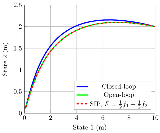
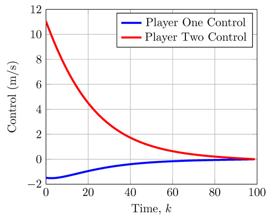
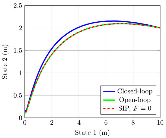
Both SIP solutions differ by less than 1% from the theoretical solution with open-loop information structure. The closed-loop information (blue), open-loop information (yellow), and SIP (red) state trajectories are shown in Figure 1. The control trajectories generated by solving the SIP formulation are shown in Figure 2 as a function of the time index k.

Figure 1. Closed-loop (blue), open-loop (green), and SIP (red) state trajectories for the two-player unconstrained convex game.

Figure 2. Control trajectories for the two-player unconstrained convex game obtained by solving the SIP.

3.1.4. SIP Numerical Results with Constrained Control

Pointwise control constraints are now added to the problem to increase the dynamic game’s complexity and demonstrate the effectiveness of the SIP approach:

$$\left|\right|u_{1,k}\left|\right|\le 3,\left|\right|u_{2,k}\left|\right|\le 3,k=0,\dots ,N-1$$

(45)

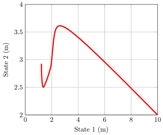
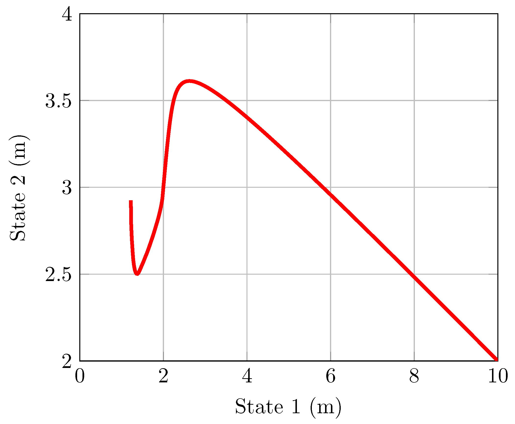
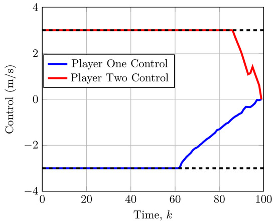
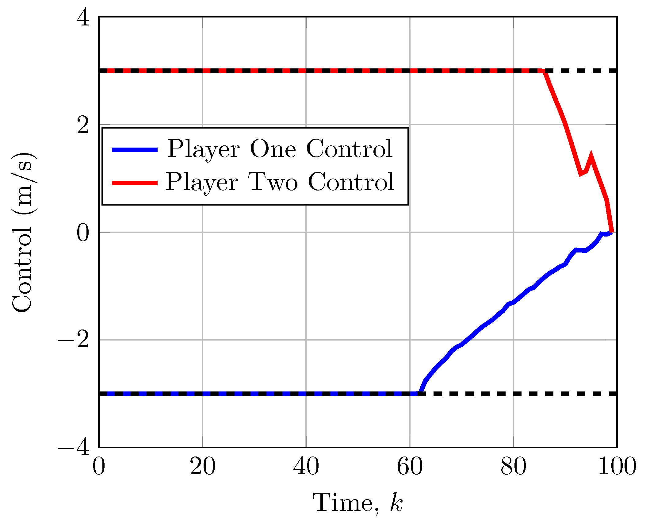
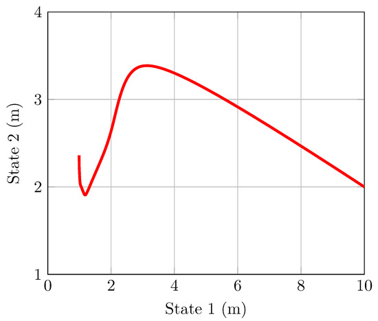
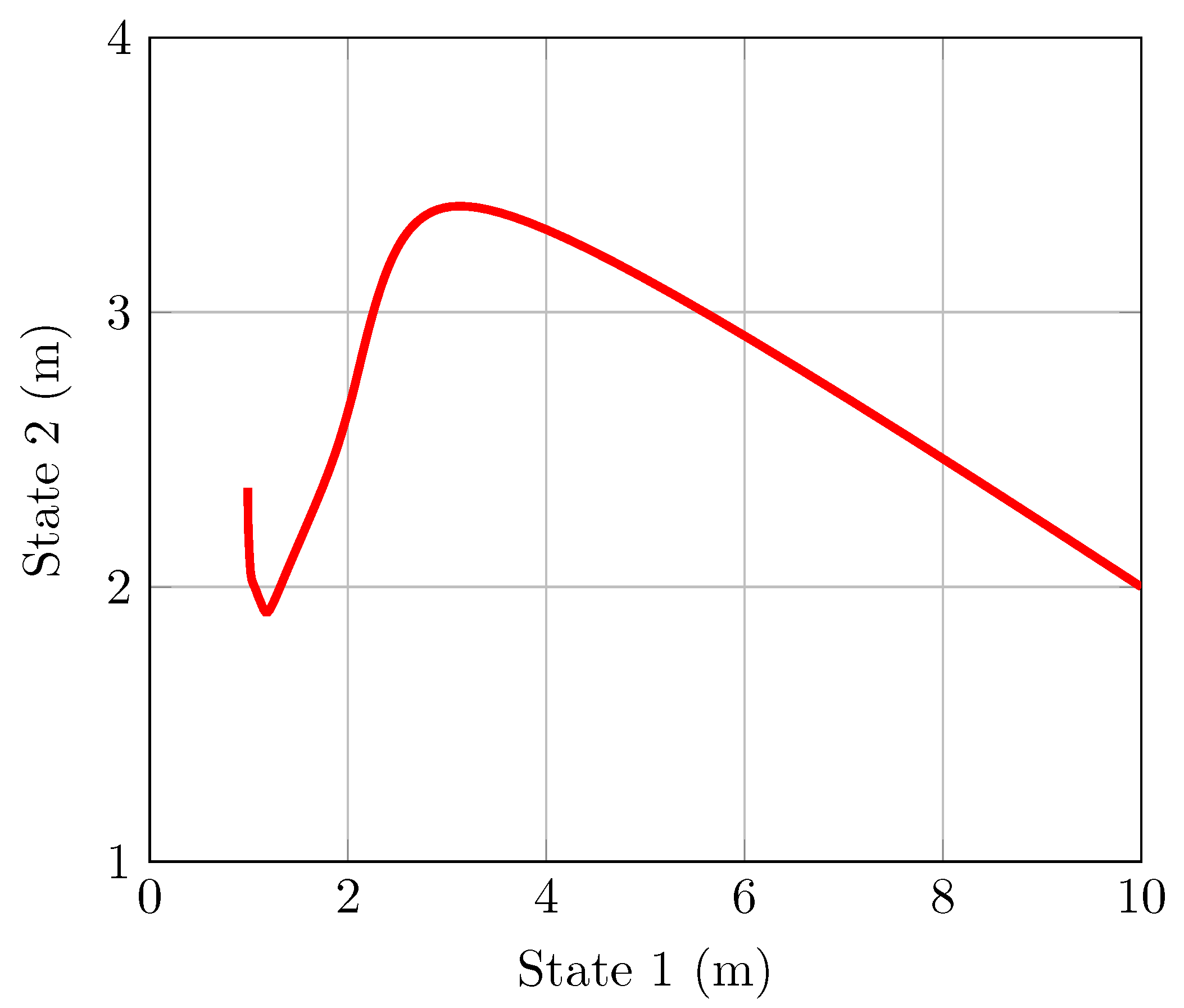
For this constrained problem, the authors are unaware of any theoretical solutions; therefore, only numerical solutions obtained from solving the SIP formulation with $F=\frac{1}{2}{f}_1+\frac{1}{2}{f}_2$ and initial guess comprised of zeros are shown. The optimal objective values are $f_1=259.436$ and $f_2=361.301$, and the iteration count is 3, taking $19.451$ s to compute. It is hypothesized that the significant reduction in run time is because the constraints effectively reduced the search space. The state trajectory is shown in Figure 3. The control trajectories are shown in Figure 4. The first player’s control is initially saturated at the lower bound, and the second player’s control is initially saturated at the upper bound.

Figure 3. State trajectory for the two-player constrained convex game obtained by solving the SIP.

Figure 4. Control trajectories for the two-player constrained convex game obtained by solving the SIP.

3.2. Three Player

A similar game with three players is now presented, solved analytically, and then solved numerically using the SIP formulation. The first player’s control at time index k is $u_{1,k}$. The second player’s control is $u_{2,k}$, and the third player’s control is $u_{3,k}$. Starting from a fixed initial condition $x_0$, they drive the following linear discrete-time system:

$$x_{k+1}=A{x}_k+B_1{u}_{1,k}+B_2{u}_{2,k}+B_3{u}_{3,k},k=0,\dots ,N-1$$

(46)

The players have the following quadratic objectives:

$$\begin{array}{cc}\hfill & f_1(u_1,u_2,u_3)=\frac{1}{2}{\displaystyle \sum _{k=0}^{N-1}}{x}_k^T{Q}_1{x}_k+u_{1,k}^T{R}_{11}{u}_{1,k}+u_{2,k}^T{R}_{12}{u}_{2,k}+u_{3,k}^T{R}_{13}{u}_{3,k}\hfill \end{array}$$

(47)

$$\begin{array}{cc}\hfill & f_2(u_1,u_2,u_3)=\frac{1}{2}{\displaystyle \sum _{k=0}^{N-1}}{x}_k^T{Q}_2{x}_k+u_{1,k}^T{R}_{21}{u}_{1,k}+u_{2,k}^T{R}_{22}{u}_{2,k}+u_{3,k}^T{R}_{23}{u}_{3,k}\hfill \end{array}$$

(48)

$$\begin{array}{cc}\hfill & f_3(u_1,u_2,u_3)=\frac{1}{2}{\displaystyle \sum _{k=0}^{N-1}}{x}_k^T{Q}_3{x}_k+u_{1,k}^T{R}_{31}{u}_{1,k}+u_{2,k}^T{R}_{32}{u}_{2,k}+u_{3,k}^T{R}_{33}{u}_{3,k}\hfill \end{array}$$

(49)

Theoretical solutions with open- and closed-loop information structures are obtained using the same techniques as in the two-player case. Numerical SIP solutions are obtained as before by initializing the finite set with 100 randomly generated sample trajectories. Rather than showing results for different choices of F, results are now shown with $F=0$ and different initializations of the internal solver: $u=0$ means controls were initialized at zero, $u=1.01u_{opt}$ means controls were initialized with random 1% variations away from the theoretical open-loop optimal solution. Table 4 shows the objective values, computation time, and iteration count for the theoretical solutions and SIP solutions. Problem data are below:

$$A=\left[\begin{array}{cc}0.893& 0.046\\ 0.033& 1.012\end{array}\right],B_1=\left[\begin{array}{c}-0.025\\ 0.019\end{array}\right],B_2=\left[\begin{array}{c}-0.003\\ -0.025\end{array}\right],B_3=\left[\begin{array}{c}-0.012\\ 0.005\end{array}\right]$$

(50)

$$Q_1=\left[\begin{array}{cc}0.169& -0.064\\ -0.064& 0.302\end{array}\right],Q_2=\left[\begin{array}{cc}0.136& -0.008\\ -0.008& 0.439\end{array}\right],Q_3=\left[\begin{array}{cc}0.140& -0.033\\ -0.033& 0.375\end{array}\right]$$

(51)

$$\begin{array}{cc}\hfill & R_{11}=0.185,R_{12}=0.060,R_{13}=0.150,R_{21}=0.110,R_{22}=0.138\hfill \end{array}$$

(52a)

$$\begin{array}{cc}\hfill & R_{23}=0.090,R_{31}=0.125,R_{32}=0.080,R_{33}=0.110\hfill \end{array}$$

(52b)

$$S_{1,N}=0,S_{2,N}=0,S_{3,N}=0$$

(53)

The initial condition is $x_0={\left[102\right]}^T$. The maximum time index is $N=100$.

Table 4. Numerical results for the three-player standard convex game.

		${\mathit{f}}_1$	${\mathit{f}}_2$	${\mathit{f}}_3$	CPU Time	Iter
Closed-loop		97.968	162.116	113.252	N/A	N/A
Open-loop		98.001	160.210	112.113	N/A	N/A
SIP	$u=0$	97.710	160.237	111.977	33.033 (min)	93
Initialization	$u=1.01u_{opt}$	97.918	160.221	111.973	10.264 (min)	40

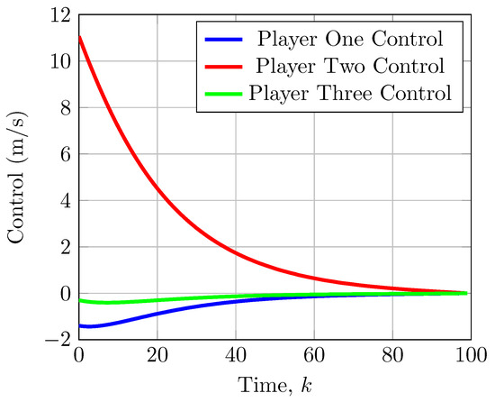
SIP solutions again approximate the theoretical solution with open-loop information structure with less than 1% error. As expected, the run time reduces dramatically when the internal solver is initialized with a high-quality guess. The closed-loop information (blue), open-loop information (yellow), and SIP (red) state trajectories are shown in Figure 5. The control trajectories generated by solving the SIP formulation are shown in Figure 6 as a function of the time index k.

Figure 5. Closed-loop (blue), open-loop (green), and SIP (red) state trajectories for the three-player unconstrained convex game.

Figure 6. Control trajectories for the three-player unconstrained convex game obtained by solving the SIP.

Pointwise control constraints are now added to the problem to increase the complexity of the dynamic game and demonstrate the effectiveness of the SIP approach:

$$\left|\right|u_{1,k}\left|\right|\le 3,\left|\right|u_{2,k}\left|\right|\le 3,\left|\right|u_{3,k}\left|\right|\le 3,k=0,\dots ,N-1$$

(54)

For this constrained problem, the authors are unaware of any theoretical solutions; therefore, only numerical solutions obtained from solving the SIP formulation with $F=0$ and initial guess comprised of zeros are shown. The optimal objective values are $f_1=249.355$, $f_2=321.853$, and $f_3=267.913$, and the iteration count is 19, taking $5.159$ min to compute. Being the largest problem solved in this paper, the timing results are compared with KKT-based approaches initialized with all zeros. Embedding the KKT conditions of players 2 and 3 as constraints in player 1’s optimization problem and solving as a nonlinear program leads to a situation in which the solver (using SQP or interior-point method) fails to converge. Embedding all players’ KKT conditions into a nonlinear program and using SQP solves in approximately 20 min. Embedding all players’ KKT conditions into a nonlinear program and using an interior-point method solves in approximately 2.5 min.

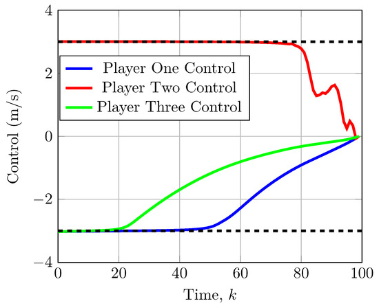
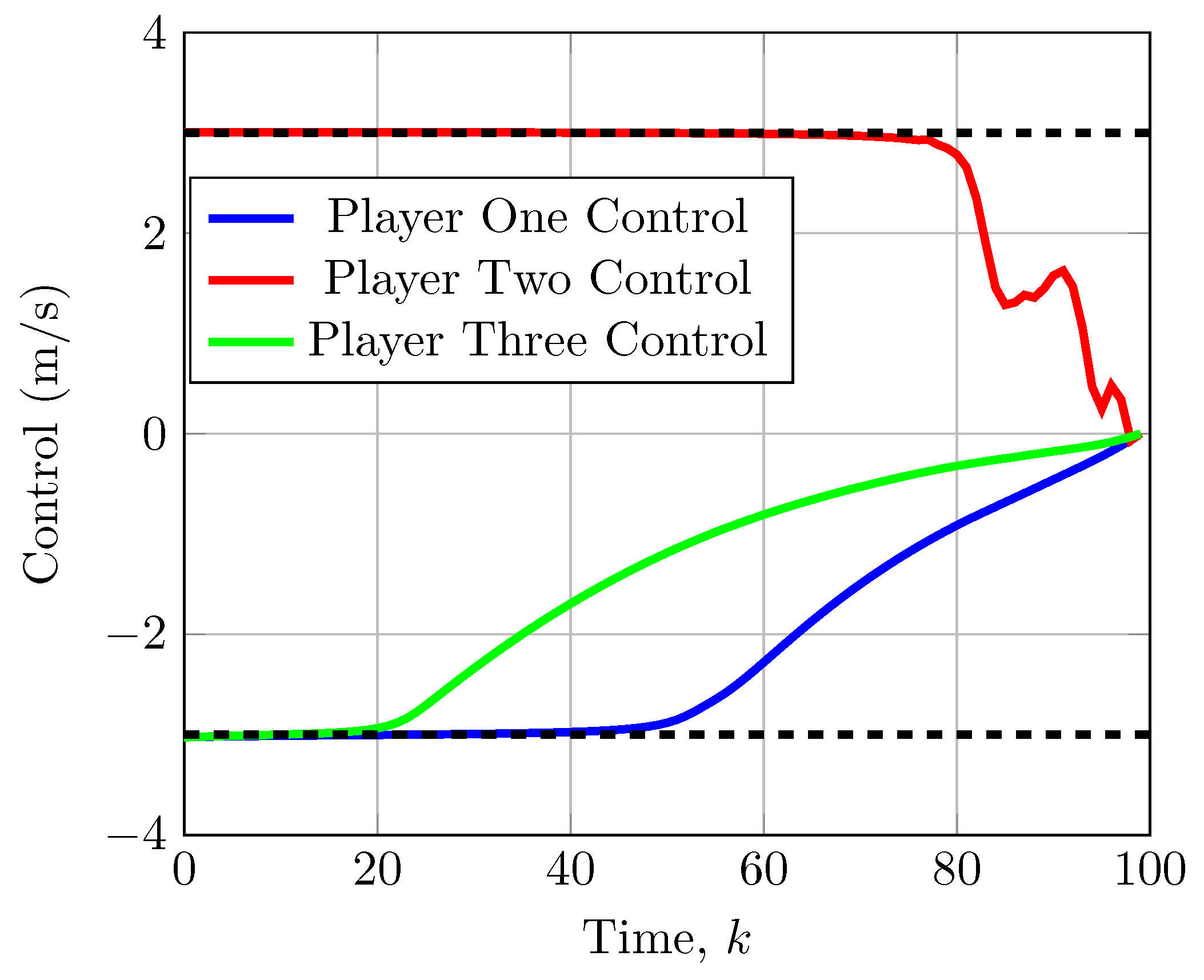
The state trajectory for the control constrained case is shown in Figure 7. The control trajectories are shown in Figure 8. The first player’s control is initially saturated at the lower bound, the second player’s control is initially saturated at the upper bound, and the third player’s control is initially saturated at the lower bound but gradually increases to zero.

Figure 7. State trajectory for the three-player constrained convex game obtained by solving the SIP.

Figure 8. Control trajectories for the three-player constrained convex game obtained by solving the SIP.

3.3. Summary of Convex Game Results

Results indicate that the proposed approach successfully solves larger-scale dynamic Nash games with hundreds of variables. The proposed approach worked with various choices of SIP objective F and various initialization strategies. As expected, higher-quality initial guesses reduced run time, but even an arbitrary initial guess led to numerical solutions with less than 1% error.

4. Nonconvex Pursuit and Evasion Dynamic Games

In the previous section, convex linear quadratic dynamic games were explored. In this section, games in which one player’s (the evader’s) objective function is nonconvex will be explored. The pursuer aims to minimize the state magnitude; the evader aims to maximize. Two games will be examined. The first is a single pursuer single evader game with running and terminal cost. The second game is a variation of the first and has only a terminal cost. The computer used to solve all problems in this section is Computer Two: 64-bit Intel Xeon(R) W-2245 at 3.90 GHz running Ubuntu 20.04.6.

4.1. Running and Terminal Cost

In this discrete-time game, the dynamics are linear and the objective functions are quadratic. The pursuer’s objective function is convex; while the evader’s is nonconvex. The objective functions are the following:

$$\begin{array}{cc}\hfill & f_p={\displaystyle \frac{1}{2}}{x}_N{S}_{p,N}{x}_N+{\displaystyle \frac{1}{2}}{\displaystyle \sum _{k=0}^{N-1}}{x}_k{Q}_p{x}_k+u_{p,k}{R}_p{u}_{p,k}\hfill \end{array}$$

(55)

$$\begin{array}{cc}\hfill & f_e=-{\displaystyle \frac{1}{2}}{x}_N{S}_{e,N}{x}_N+{\displaystyle \frac{1}{2}}{\displaystyle \sum _{k=0}^{N-1}}-x_k{Q}_e{x}_k+u_{e,k}{R}_e{u}_{e,k}\hfill \end{array}$$

(56)

Dynamics are described by the following equation:

$$\begin{array}{cc}\hfill & x_{k+1}=A{x}_k+B_p{u}_{p,k}+B_e{u}_{e,k}\hfill \end{array}$$

(57)

Theoretical solutions with open- and closed-loop information structures are obtained as before. Problem data are given below where I is the 2-by-2 identity matrix:

$$\begin{array}{cc}\hfill & A=I,B_p=-B_e=0.03I\hfill \end{array}$$

(58)

$$\begin{array}{cc}\hfill & Q_p=I,Q_e=0.1I,R_p=I,R_e=2I\hfill \end{array}$$

(59)

$$\begin{array}{cc}\hfill & S_{p,N}=S_{e,N}=0\hfill \end{array}$$

(60)

$$\begin{array}{cc}\hfill & x_0={[-3-1]}^T,N=100\hfill \end{array}$$

(61)

The SIP algorithm is initialized with a finite set comprised of 100 randomly generated sample trajectories, and the internal solver fmincon initialized with controls set to zero. Four SIP objective functions are considered: $F=f_p$, $F=f_e$, $F={\sum }_{k=0}^{N-1}\left|\right|u_{p,k}+u_{e,k}{\left|\right|}^2$, and $F=\frac{1}{2}{f}_p+\frac{1}{2}{f}_e$. Table 5 shows the results.

Table 5. Numerical results for the one evader one pursuer game.

		${\mathit{f}}_{\mathit{p}}$	${\mathit{f}}_{\mathit{e}}$	CPU Time	Iter
Closed-loop		172.774	8.924	N/A	N/A
Open-loop		176.819	9.478	N/A	N/A
SIP	$F=\frac{1}{2}{f}_p+\frac{1}{2}{f}_e$	172.149	8.975	2.427 (min)	3
Objective	$F=f_p$	174.125	9.066	$67.200$ (min)	7
	$F=f_e$	176.760	9.484	37.6793 (min)	21
	$F={\sum }_{k=0}^{N-1}\left|\right|u_{p,k}+u_{e,k}{\left|\right|}^2$	177.490	9.692	220.440 (min)	26

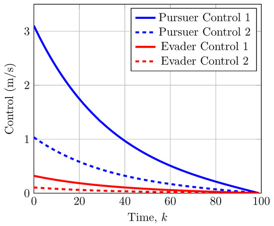
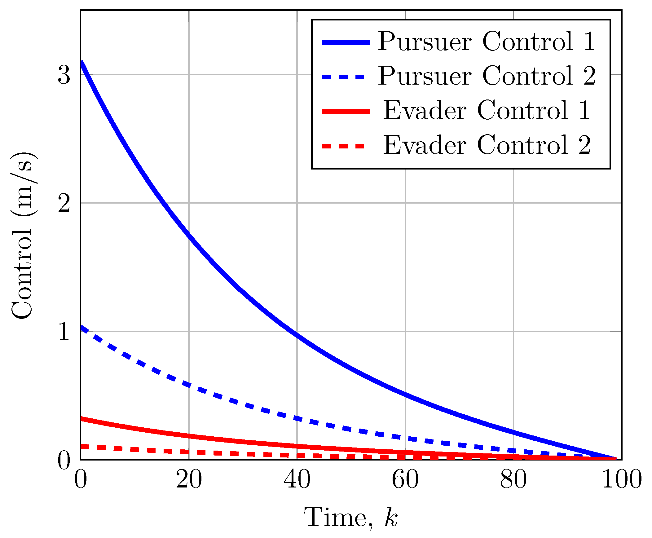
For the problem data used, all six solutions are visually indistinguishable. Comparative plots are not shown for this reason. The optimal controls obtained by solving the SIP with $F=f_e$ are shown in Figure 9. There are four curves because each player’s control vector is two-dimensional.

Figure 9. Control trajectories for the single pursuer running distance obtained by solving the SIP.

4.2. Terminal Cost

In this final scenario, the objective of the pursuer is to minimize the magnitude of the final state, and the objective of the evader is to maximize the magnitude of the final state. To demonstrate efficacy of the SIP formulation and selected algorithm in the broader field of game theory, this pursuit–evasion game is modeled as a sequential game in which the evader plays first and the pursuer plays second. The dynamics are again linear. The pursuer’s control must belong to the set ${\mathcal{U}}_p$, and the evader’s control must belong to the set ${\mathcal{U}}_e$:

$$\begin{array}{cc}\hfill \underset{u_e\in {\mathcal{U}}_e}{min}& -\left|\right|x_N{\left|\right|}^2\hfill \end{array}$$

(62a)

$$\begin{array}{cc}\hfill \mathrm{subj}.\mathrm{to}& \underset{u_p\in {\mathcal{U}}_p}{min}\left|\right|x_N{\left|\right|}^2\hfill \end{array}$$

(62b)

$$\begin{array}{cc}\hfill & \mathrm{subj}.\mathrm{to}{x}_{k+1}=A{x}_k+B_p{u}_{p,k}+B_e{u}_{e,k}\hfill \end{array}$$

(62c)

$$\begin{array}{cc}\hfill & x_0\mathrm{given}\hfill \end{array}$$

(62d)

As was done in Section 2, replacing the pursuer’s minimization with inequalities converts the sequential game into a SIP.

$$\begin{array}{cc}\hfill \underset{u_e\in {\mathcal{U}}_e,u_e\in {\mathcal{U}}_e}{min}& -\left|\right|x_N{\left|\right|}^2\hfill \end{array}$$

(63a)

$$\begin{array}{cc}\hfill \mathrm{subj}.\mathrm{to}& \left|\right|x_N{\left|\right|}^2\le \left|\right|{\chi }_N{\left|\right|}^2\hfill \end{array}$$

(63b)

$$\begin{array}{cc}\hfill & x_{k+1}=A{x}_k+B_p{u}_{p,k}+B_e{u}_{e,k}\hfill \end{array}$$

(63c)

$$\begin{array}{cc}\hfill & {\chi }_{k+1}={\chi }_k+B_p{\mu }_{p,k}+B_e{u}_{e,k},\forall {\mu }_{p,k}\in {\mathcal{U}}_p\hfill \end{array}$$

(63d)

$$\begin{array}{cc}\hfill & x_0\mathrm{given}\hfill \end{array}$$

(63e)

The semi-infinite variables are the ${\mu }_{p,k}$ for $k=0,\dots ,N-1$.

For the numerical example, the following data are used:

$$\begin{array}{cc}\hfill & A=B_p=-B_e=I,-1\le u_{p,k}\le 1,-1\le u_{e,k}\le 1,x_0={\left[66\right]}^T\hfill \end{array}$$

(64)

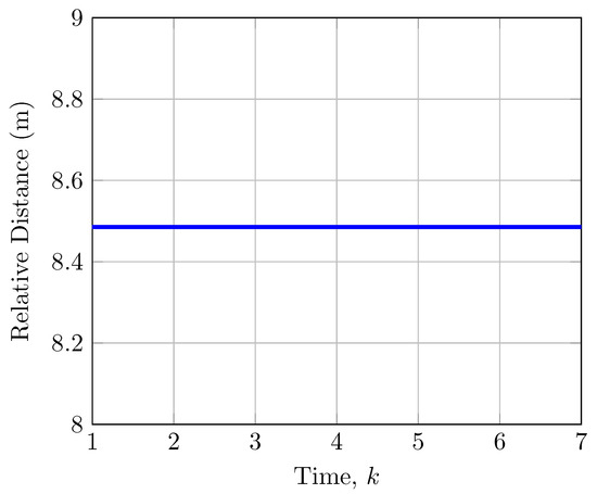
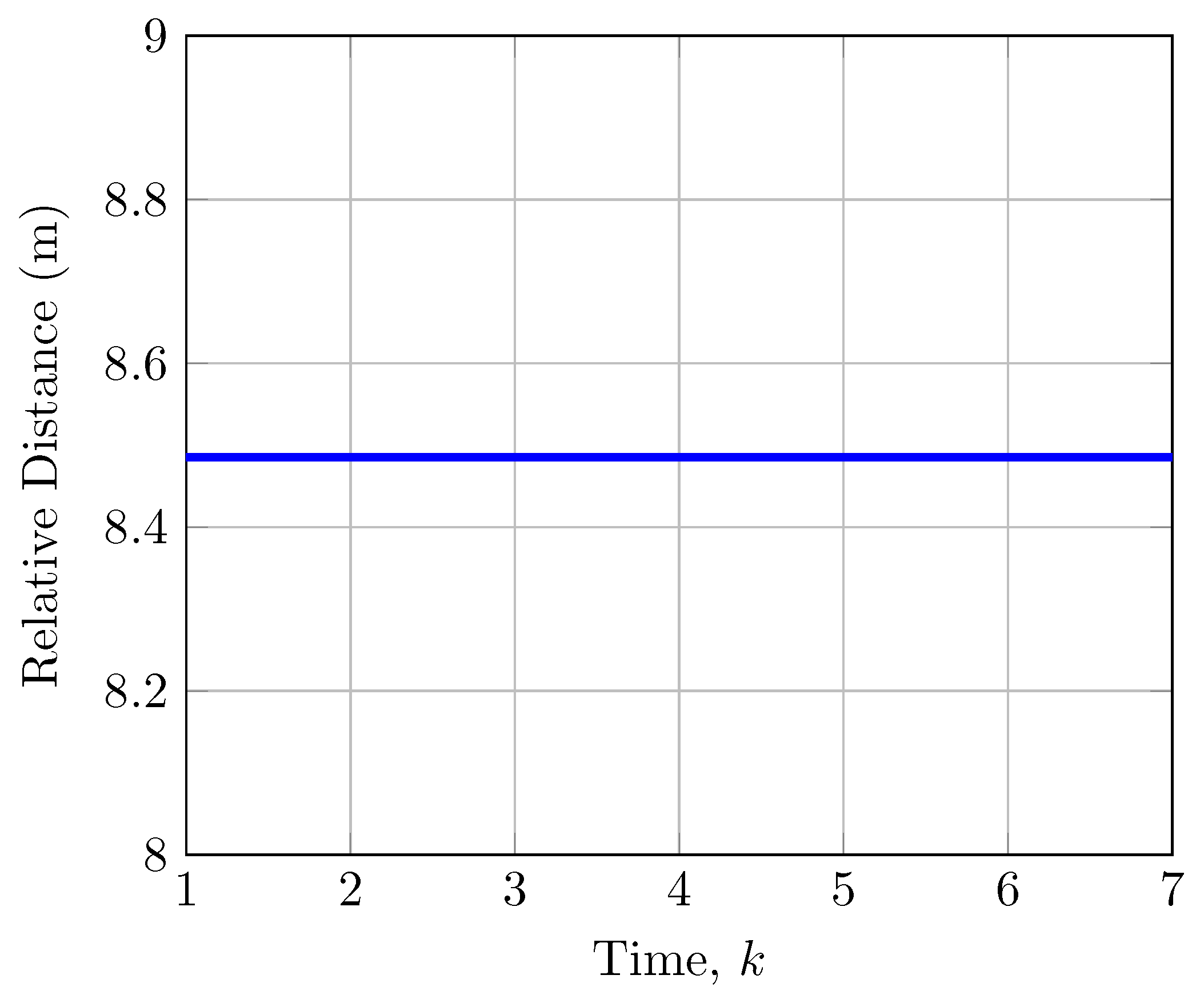
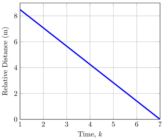
The SIP algorithm is initialized with a finite set comprised of 100 sample trajectories, and the internal solver fmincon is initialized with controls set to their maximum allowed value. The algorithm converges to a solution in 0.086 s after two iterations. The magnitude of the state $\left|\right|x_k\left|\right|$ is shown in Figure 10. As expected, the magnitude is constant because the two players have equal control authority and their control matrices are equal and opposite. The best strategy for the evader is to control at the maximum allowed level, and similarly for the pursuer.

Figure 10. Relative distance for the final distance formulation without capture by solving the SIP.

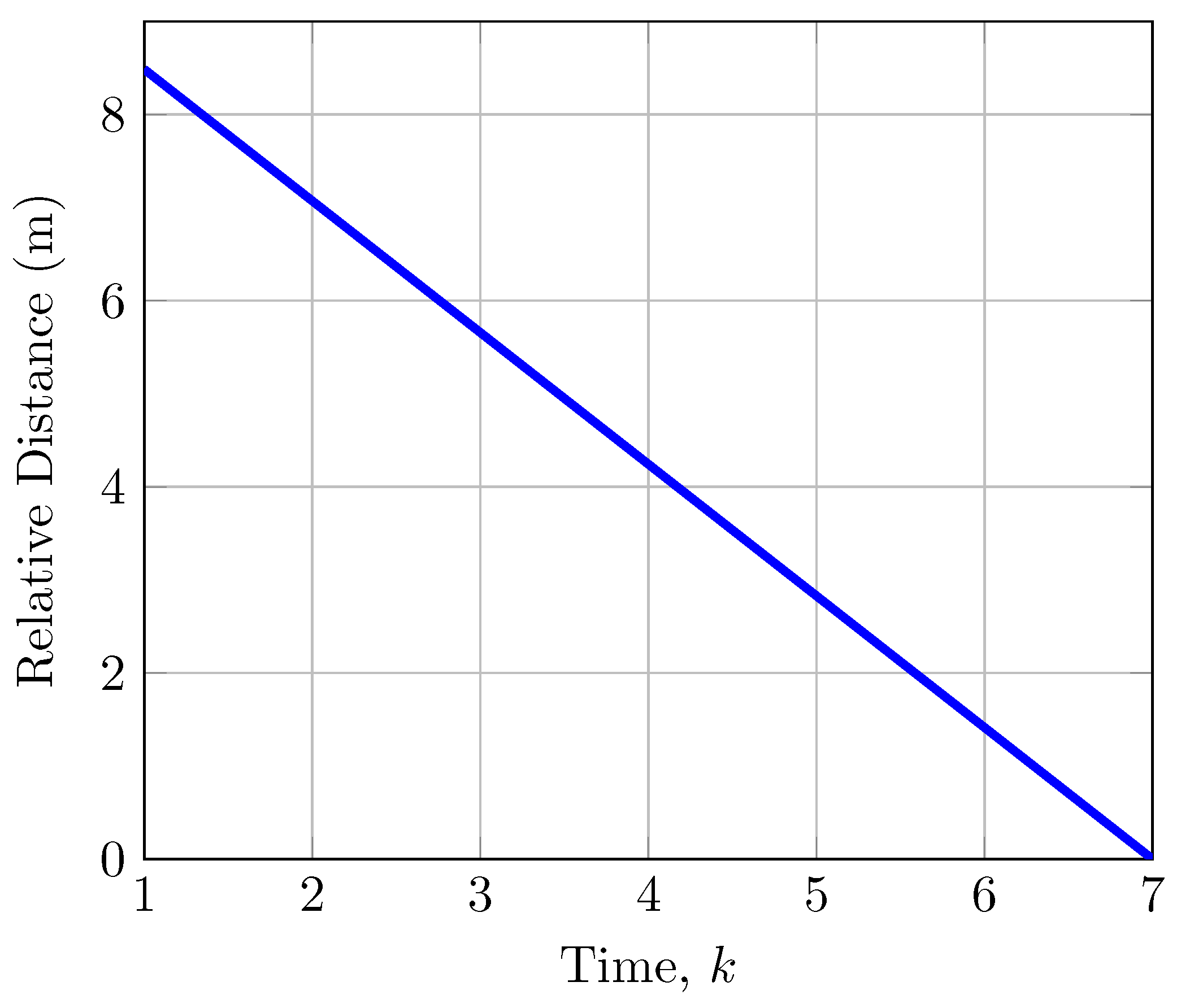
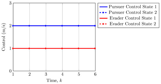
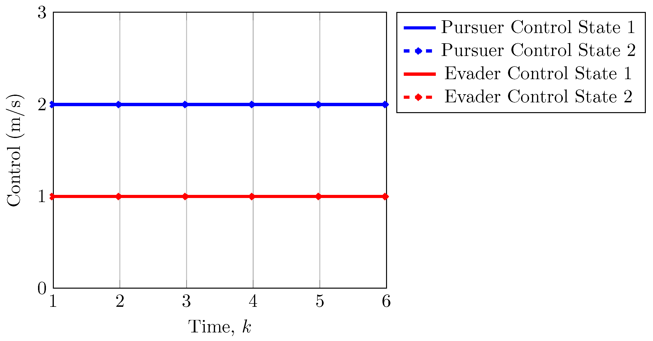
Increasing the pursuer’s control authority to $-2\le u_{p,k}\le 2$ allows capture to occur, i.e., $\left|\right|x_N\left|\right|=0$. Initialized as before, the SIP algorithm converges in 248.092 s after 486 iterations. The state magnitude as a function of time is shown in Figure 11. The magnitude decreases linearly to zero at the final time. The control trajectories generated by solving the SIP are shown in Figure 12. As expected, the optimal controls remain at the extreme values of their feasible sets.

Figure 11. Relative state distance for the final distance formulation with capture by solving the SIP.

Figure 12. Control trajectories for the final distance constrained with capture obtained by solving the SIP.

4.3. Summary of Nonconvex Game Results

Applied to pursuit–evasion games, the SIP approach successfully solved problems formulated as a Nash game and a sequential game. Within the Nash game, four SIP objectives were considered. While the CPU solve time varied dramatically, all solutions approximated the known theoretical solutions. Within the sequential game, two scenarios were considered wherein the players had equal control authority and unequal control authority. As expected, capture occurred in the latter but not the former.

5. Conclusions

With the goal of numerically solving Nash games, the paper presented: (1) transformation of a Nash game into a numerically solvable SIP; (2) identification of a suitable SIP solver that generates a provably $ϵ$-optimal Nash solution; and (3) successful demonstration on benchmark problems and larger-scale dynamic games. Compared to common alternative approaches, the approach described herein does not use KKT conditions, and thus avoids the challenges associated with them. The approach does involve solving a sequence of nonconvex programs that must be solved at least locally to ensure convergence to an $ϵ$-optimal point. This limits the speed and size of problems that are solvable. On the other hand, as nonconvex solvers advance, they can easily be incorporated into the algorithm.

In numerical experiments, various SIP objectives, algorithm initializations, and internal solver initializations were considered and shown to have minimal effects on solution quality but large effects on run time. For problems with known analytical solutions, numerical solutions were within approximately one percent. In one problem, changing SIP objectives caused run times to vary by a factor of 100.

Future work could focus on parallelized implementations for games with a large number of players, particularly a simultaneous solution for the lower-level problem across players. Though feasible initial guesses are not needed, customizing initialization strategies for a given problem may significantly reduce run times. Lastly, further applying optimization best practices is expected to accelerate solve times. The results presented herein were not obtained by fine-tuning every knob. For a given problem, it is expected that performance can be enhanced by customization.

References

- Başar, T., & Olsder, G. J. (1999). Dynamic noncooperative game theory. SIAM. [Google Scholar]
- Ben-Tal, A., & Nemirovski, A. (1999). Robust solutions of uncertain linear programs. Operations Research Letters, 25(1), 1–13. [Google Scholar] [CrossRef] [Scilit]
- Berkovitz, L. D. (2002). Convexity and optimization in ℝn. John Wiley and Sons, Inc. [Google Scholar]
- Bhattacharjee, B., Green, W. H., & Barton, P. I. (2005a). Interval methods for semi-infinite programs. Computational Optimization and Applications, 30(1), 63–93. [Google Scholar] [CrossRef] [Scilit]
- Bhattacharjee, B., Lemonidis, P., Green, W. H., Jr., & Barton, P. I. (2005b). Global solution of semi-infinite programs. Mathematical Programming, 103(2), 283–307. [Google Scholar] [CrossRef] [Scilit]
- Bryson, A. E., & Ho, Y.-C. (1975). Applied optimal control. Hemisphere. [Google Scholar]
- Cerulli, M., Oustry, A., D’Ambrosio, C., & Liberti, L. (2022). Convergent algorithms for a class of convex semi-infinite programs. SIAM Journal on Optimization, 32(4), 2493–2526. [Google Scholar] [CrossRef] [Scilit]
- Chenchene, E., Huang, H., & Qiu, J. (2025). A consensus-based algorithm for non-convex multiplayer games. Journal of Optimization Theory and Applications, 206(2), 45. [Google Scholar] [CrossRef] [Scilit]
- Colombo, R. M., Giuzzi, L., & Marcellini, F. (2025). Nash equilibria in traffic networks with multiple populations and origins–destinations. Journal of Optimization Theory and Applications, 206(2), 31. [Google Scholar] [CrossRef] [Scilit]
- Djelassi, H., Mitsos, A., & Stein, O. (2021). Recent advances in nonconvex semi-infinite programming: Applications and algorithms. EURO Journal on Computational Optimization, 9, 100006. [Google Scholar] [CrossRef] [Scilit]
- Engwerda, J. (2018). Stabilization of an uncertain simple fishery management game. Fisheries Research, 203, 63–73. [Google Scholar] [CrossRef] [Scilit]
- Feng, Z., Chen, F., Chen, L., & Yiu, K. F. C. (2020). Optimality analysis of a class of semi-infinite programming problems. Journal of Optimization Theory and Applications, 186(2), 398–411. [Google Scholar] [CrossRef] [Scilit]
- Floudas, C. A., & Stein, O. (2008). The adaptive convexification algorithm: A feasible point method for semi-infinite programming. SIAM Journal on Optimization, 18(4), 1187–1208. [Google Scholar] [CrossRef] [Scilit]
- Garagic, D., & Cruz, J., Jr. (2003). An approach to fuzzy noncooperative Nash games. Journal of Optimization Theory and Applications, 118(3), 475–491. [Google Scholar] [CrossRef] [Scilit]
- Guo, P., Wang, Y., & Li, H. (2013). A semi-tensor product approach to finding Nash equilibria for static games. In Proceedings of the 32nd Chinese control conference (pp. 107–112). IEEE. [Google Scholar]
- Gurobi Optimization, LLC. (2024). Gurobi optimizer reference manual, version 11.0.3. Available online: https://www.gurobi.com (accessed on 28 May 2026).
- Harris, M. W., & Rose, M. B. (2023). Optimal spacecraft guidance. Utah State University. [Google Scholar]
- Hayashi, S., & Wu, S.-Y. (2010). An explicit exchange algorithm for linear semi-infinite programming problems with second-order cone constraints. SIAM Journal on Optimization, 20(3), 1527–1546. [Google Scholar] [CrossRef] [Scilit]
- Hettich, R., & Kortanek, K. O. (1993). Semi-infinite programming: Theory, methods, and applications. SIAM Review, 35(3), 380–429. [Google Scholar] [CrossRef] [Scilit]
- Huang, Y., & Zhao, J. (2021). Socially optimal Nash equilibrium of switched linear quadratic differential games. In 2021 40th Chinese control conference (CCC) (pp. 1425–1430). IEEE. [Google Scholar] [CrossRef] [Scilit]
- Isaacs, R. (1965). Differential games: A mathematical theory with applications to warfare and pursuit, control and optimization. John Wiley and Sons. [Google Scholar]
- Krieg, H., Seidel, T., Schwientek, J., & Küfer, K.-H. (2022). Solving continuous set covering problems by means of semi-infinite optimization. Mathematical Methods of Operations Research, 96(1), 39–82. [Google Scholar] [CrossRef] [Scilit]
- Lin, T., Jin, C., & Jordan, M. (2020). On gradient descent ascent for nonconvex-concave minimax problems. In Proceedings of the 37th international conference on machine learning (pp. 6083–6093). PMLR. [Google Scholar]
- Ling, C., Qi, L. Q., Zhou, G. L., & Wu, S. Y. (2006). Global convergence of a robust smoothing SQP method for semi-infinite programming. Journal of Optimization Theory and Applications, 129(1), 147–164. [Google Scholar] [CrossRef] [Scilit]
- López, M., & Still, G. (2007). Semi-infinite programming. European Journal of Operational Research, 180(2), 491–518. [Google Scholar] [CrossRef] [Scilit]
- Mitsos, A. (2011). Global optimization of semi-infinite programs via restriction of the right-hand side. Optimization, 60(10–11), 1291–1308. [Google Scholar] [CrossRef] [Scilit]
- Mitsos, A., Lemonidis, P., Lee, C. K., & Barton, P. I. (2008). Relaxation-based bounds for semi-infinite programs. SIAM Journal on Optimization, 19(1), 77–113. [Google Scholar] [CrossRef] [Scilit]
- Mylvaganam, T., & Astolfi, A. (2015). Control of microgrids using a differential game theoretic framework. In 2015 54th IEEE conference on decision and control (CDC) (pp. 5839–5844). IEEE. [Google Scholar] [CrossRef] [Scilit]
- Nouiehed, M., Sanjabi, M., Huang, T., Lee, J. D., & Razaviyayn, M. (2019). Solving a class of non-convex min-max games using iterative first order methods. In Advances in neural information processing systems 32 (NeurIPS 2019). Curran Associates, Inc. [Google Scholar]
- Pang, L.-P., & Wu, Q. (2022). A feasible proximal bundle algorithm with convexification for nonsmooth, nonconvex semi-infinite programming. Numerical Algorithms, 90(1), 387–422. [Google Scholar] [CrossRef] [Scilit]
- Polak, E., & Stimler, D. (1988). Majorization: A computational complexity reduction technique in control system design. IEEE Transactions on Automatic Control, 33(11), 1010–1021. [Google Scholar] [CrossRef] [Scilit]
- Pontani, M., & Conway, B. A. (2009). Numerical solution of the three-dimensional orbital pursuit-evasion game. Journal of Guidance, Control, and Dynamics, 32(2), 474–487. [Google Scholar] [CrossRef] [Scilit]
- Ratliff, L. J., Burden, S. A., & Sastry, S. S. (2013). Characterization and computation of local Nash equilibria in continuous games. In 2013 51st annual allerton conference on communication, control, and computing (Allerton) (pp. 917–924). IEEE. [Google Scholar] [CrossRef] [Scilit]
- Ratliff, L. J., Burden, S. A., & Sastry, S. S. (2016). On the characterization of local Nash equilibria in continuous games. IEEE Transactions on Automatic Control, 61(8), 2301–2307. [Google Scholar] [CrossRef] [Scilit]
- Stein, O. (2006). A semi-infinite approach to design centering. In Optimization with multivalued mappings: Theory, applications, and algorithms (pp. 209–228). Springer US. [Google Scholar] [CrossRef] [Scilit]
- Tang, W., & Daoutidis, P. (2023). Optimal design of control-Lyapunov functions by semi-infinite stochastic programming. In 2023 62nd IEEE conference on decision and control (CDC) (pp. 7277–7284). IEEE. [Google Scholar] [CrossRef] [Scilit]
- Taylor, P. D., & Jonker, L. B. (1978). Evolutionary stable strategies and game dynamics. Mathematical Biosciences, 40(1), 145–156. [Google Scholar] [CrossRef] [Scilit]
- The MathWorks Inc. (2024). MATLAB R2024a (Version 24.1). The MathWorks Inc. Available online: https://www.mathworks.com (accessed on 28 May 2026).
Disclaimer/Publisher’s Note: The statements, opinions and data contained in all publications are solely those of the individual author(s) and contributor(s) and not of MDPI and/or the editor(s). MDPI and/or the editor(s) disclaim responsibility for any injury to people or property resulting from any ideas, methods, instructions or products referred to in the content. |
© 2026 by the authors. Licensee MDPI, Basel, Switzerland. This article is an open access article distributed under the terms and conditions of the Creative Commons Attribution (CC BY) license.