Measuring Pitcher Production Fairly in Baseball Using the Shapley Value

Abstract

This paper introduces fairer measures of individual pitcher performance in baseball using the Shapley Value from coalitional game theory. The paper’s key conceptual innovation is a novel two-stage procedure for constructing the coalitionary game value functions for runs allowed and outs recorded by a baseball team’s defense. This procedure enables the Shapley Value calculation to fairly divide credit for runs and outs between different pitchers and between pitchers and fielders. It also results in two new statistics—Shapley Pitcher Runs (SPR) and Shapley Pitcher Outs (SPO)—that, unlike traditional pitching statistics, consistently satisfy several mathematical fairness axioms. A third statistic, called Shapley Run Average, provides a fairer measure of pitcher efficiency. I calculate these statistics for the 2022 Major League Baseball regular season and the 1955–2022 World Series championships. Using SPR and SPO as the standard for fairness, empirical analysis reveals that the traditional pitching statistics systematically and unfairly overcredit pitchers by 40–50%, with starting pitchers miscredited more severely than relievers. Analysis of SRA identifies efficient pitchers whose performance is obscured by conventional statistics and enables a reassessment of historic World Series performances. Overall, this work demonstrates another application of the Shapley Value to creating new performance measures in team sports.

1. Introduction

Performance measures are used in many professions, from allocating bonuses among coworkers to selecting the winner of a school’s teaching award. However, it is especially difficult to accurately measure individual performance in team settings in which the outcome is the result of the complex interplay of many individuals’ contributions. Simple measures of inputs such as time spent working will not accurately measure performance; instead, each person’s contribution must be isolated in a way that respects the collaborative nature of the endeavor.

This is especially true in team sports. Indeed, the challenge of how to fairly allocate credit and blame has been recognized in baseball since 1867, when the “Father of Baseball” Henry Chadwick grappled with how to fairly assign credit (blame) to pitchers for runs that score when they pitch. His solution was the earned run statistic, which absolves the pitcher of blame for runs that score as a result of fielding errors (Schwarz, 1994). However, the earned run statistic is unfair in fully blaming the pitcher who allowed a runner on base when that runner scored against another pitcher, and in counting all earned runs the same whether or not fielding was involved. Meanwhile, the innings pitched statistic unfairly credits the pitcher for all outs recorded whether or not fielding was involved. Although there have been several advances in measuring pitcher performance, the fundamental approach to crediting pitchers for runs and outs has remained unchanged despite inherent unfairness.

This paper addresses three questions: (1) How should baseball pitchers be fairly credited for runs allowed and outs recorded when outcomes result from collaboration between pitchers and fielders and between multiple pitchers? (2) How do new measures of credit that more fairly account for collaboration compare with existing measures? (3) What insights do these improved measures provide about pitching performances in Major League Baseball?

To answer the first question, I develop a new method for assigning credit to pitchers that uses the Shapley Value concept from coalitional game theory (Shapley, 1953). This approach produces three new measures: Shapley Pitcher Runs (SPR), Shapley Pitcher Outs, and Shapley Run Average (SRA). SPR and SPO are calculated after mathematically representing runs allowed and outs recorded as coalitional games involving pitchers and fielders. As Shapley Values, SPR and SPO satisfy established theoretical fairness axioms that existing pitching statistics do not consistently meet. Thus, SRA provides a theoretically grounded alternative to earned-run average (ERA) to assess pitcher efficiency.

To answer the second and third questions, I calculate SPR, SPO, and SRA for the 2022 Major League Baseball regular season and the 1955–2022 World Series. Analysis of the calculations finds that: (1) traditional pitcher statistics systematically overcredit pitchers by 40–$50\%$; (2) overcrediting of runs affects starting pitchers more severely than relief pitchers; (3) SRA identifies pitchers whose efficiency is not accurately reflected in statistics such as ERA and fielding-independent pitching (FIP); and (4) SRA identifies the best World Series pitcher performances, thereby enabling a reevaluation of historically significant pitcher performances.

This paper contributes to two distinct literatures, the first being applications of the Shapley Value, see Algaba (2020). A small subset of this literature examines sports. For example, Fletcher-Hill (2014) and Hiller (2015) use the Shapley Value to estimate soccer players’ productivity; Metulini and Gnecco (2023) use the Shapley Value to estimate players’ expected contributions to winning; and van den Brink and Gilles (2000) and Manuel et al. (2013) use the Shapley Value to rank teams based on wins and losses.

McBride (2026) provides the only previous application of the Shapley Value to baseball. He (i) introduced a framework in which mathematically rich “event triggers,” that he created for past Major League Baseball games using machine learning models, replace baseball play events to replicate hypothetical innings, and he (ii) showed how event triggers could be selected for and then sequenced through for a coalition of offensive players to obtain a value-function value for that coalition. Completing the sequencing in (ii) using the event triggers from (i) for each coalition of players produced a well-defined coalitional game theory value function. Shapley Values were then calculated using these value functions to obtain his Shapley Run Credit statistic for baseball offense.

In this paper, I use his event-trigger framework and machine learning event triggers from (i), but his method for selecting event triggers for offensive players in (ii) cannot be applied to baseball defense because it does not account for the different roles of pitchers and fielders. I introduce a novel two-stage procedure to accomplish (ii) for baseball defense, i.e., a method that produces value functions from which Shapley Values can be calculated that respect the different pitching and fielding roles. The two-stage procedure is the main conceptual contribution of the paper and demonstrates another way in which the Shapley Value can be applied to team sports.

The second literature consists of baseball analytics research (“sabermetrics”). This work spans a variety of topics, such as the business side of baseball (e.g., Ormiston, 2014; Pifer et al., 2020; Solow & Krautmann, 2020), the measurement of player performance (e.g., James & Henzler, 2002; Schwarz, 1994; Thorn & Palmer, 2015), prediction (e.g., Doo & Kim, 2018; Tango et al., 2007), and more. My work contributes to the research on pitching (e.g., Baldini et al., 2011; Sidle & Tran, 2018) and follows in the footsteps of McCracken (2001) who inspired the creation of fielding-independent pitching statistics. Similar to these pitching statistics, the Shapley pitching statistics treat outcomes differently based on whether fielding was involved, but they do so using mathematical fairness axioms built into the Shapley Value. This gives the Shapley pitching statistics presented here a unique theoretical grounding and justification that no other pitching statistics can claim.

The focus on fair assignment of credit also distinguishes this paper from recent developments in estimating pitcher skill. While skill estimation aims to predict future performance for roster construction and in-game strategic decisions, credit assignment seeks an accurate measurement of past performance. These objectives are related because skill estimates depend partly on the quality of the underlying credit statistics (e.g., ERA combines the earned run and innings pitched credit measures). As credit measures, SPR, SPO, and SRA are not designed directly to improve prediction, but instead are designed to be the fairest and most accurate measures of actual performance.

Finally, note that SPR, SPO, and SRA can also be calculated for pitchers in fastpitch softball and slowpitch softball, two team sports that have very similar rules as baseball.

2. A Primer on SPR, SPO, and SRA

This section provides a non-technical introduction to the new Shapley pitching statistics, illustrating how they more fairly account for pitcher–pitcher and pitcher–fielder collaboration. A typical (professional) baseball game lasts nine innings, where each inning consists of each team taking a turn on both defense and offense. Because the Shapley statistics are constructed and calculated inning by inning, in this section we only consider an example of just a single half-inning (hereafter inning). The same logic would be applied to every inning of a game to obtain the statistics for that entire game.

Table 1 lists the play events for a single inning in which three runs are scored against two pitchers. For each play event, the columns report the pitcher, the play outcome, whether fielding was involved, the number of runs scored, and the number of outs recorded. The first several columns of Table 2 provide pitching statistics for that inning that are included in a typical box-score summary. The runs allowed (R) statistic assigns full credit for all three runs that scored to Pitcher A because the players who scored reached base against Pitcher A, but only two of the runs are earned runs due to the fielding error. FIP is a fielding-independent estimator of a pitcher’s ERA. ERA and FIP are most valuable when calculated for many games, but both are provided here for comparison.

Table 1. The Two-Pitcher Inning.

Pitcher	Play	Fielding	Runs	Earned Runs	Outs
A	Reached first base on fielding error	Yes	0	0	0
A	Home run	No	2	1	0
A	Strikeout	No	0	0	1
A	Double	Yes	0	0	0
B	Double, RBI	Yes	1	1	0
B	Strikeout	No	0	0	1
B	Groundout	Yes	0	0	1

Table 2. Box score for the Two-Pitcher Inning.

Pitcher	IP	R	ER	H	BB	K	HR	ERA	FIP	SPR	SPO	SRA
A	0.1	3	2	2	0	1	1	54.00	36.20	1.75	1.00	47.25
B	0.2	0	0	1	0	1	0	0.00	0.20	0.25	1.50	4.50
Total	1	3	2	3	0	2	1	18.00	12.20	2.00	2.50	21.60

Notes: IP = innings pitched, R = runs allowed, ER = earned runs allowed, H = hits allowed, BB = walks allowed, K = strikeouts allowed, HR = home runs allowed, ERA = earned-run average, FIP = fielding-independent pitching (assumes 3.20 FIP constant), SPR = Shapley pitcher runs, SPO = Shapley pitcher outs, SRA = Shapley run average. 0.1 IP denotes one-third of an inning pitched, and 0.2 denotes two-thirds of an inning pitched.

The last three columns of Table 2 provide the new Shapley pitching statistics. A pitcher’s Shapley Pitcher Runs (SPR) is their Shapley Value from a coalitional game in which the value function measures runs that are allowed to score, i.e., SPR is their fair share of credit (blame) for the runs their team’s defense allowed to score. According to SPR, Pitcher A is fully responsible for the run scored by the home run (HR) because the fielders could not do anything to prevent it, but SPR splits the credit for the other two runs between the two pitchers and fielders. Because the leadoff batter reached base via a fielded ball in play, Pitcher A and the fielders (i.e., the fielders as a collective entity) are calculated by the Shapley Value to be equally responsible for that leadoff runner reaching base and eventually scoring. By the Shapley Value calculation, credit for the third run is split equally between the fielders and the collective pitchers, and the pitchers’ collective share is split equally between the two pitchers because both pitchers participated in that scored run. Summing these credits yields $2.00$ SPR for the pitchers collectively in this inning, with $1.75$ SPR for Pitcher A ($0.50+1.00+0.25$) and $0.25$ SPR for Pitcher B ($0+0+0.25$). The remaining $1.00$ run of credit for this inning is attributed to the fielders, so the total amount credited to the pitchers and fielders exactly equals the total of three runs scored in the inning.

SPR partitions the credit for runs more fairly than runs (R) and earned runs (ER). First, SPR assigns full credit to the pitcher for runs that did not involve fielding, but it divides the credit between pitchers and fielders when batters reach base on fielding plays. The pitcher gets some credit when there is a fielding error because the pitcher allowed the ball in play. Second, SPR divides the credit between different pitchers when a batter reaches base against one pitcher but scores against a different pitcher. The total SPR and earned runs both happen to be two runs in this example, but because most of the runs in a typical game are earned, earned runs will usually assign more credit to pitchers than SPR.

Shapley Pitcher Outs (SPO) are Shapley Values for a coalitional game for outs recorded. Pitcher A is credited with $1.00$ SPO in this inning because their strikeout did not involve a ball in play. Pitcher B similarly gets full credit for their strikeout, but splits the credit with the fielders for the ground-out for a total of $1.50$ SPO. The remaining $0.50$ outs for the three-out inning are credited to the fielders.

SPO credits pitchers for outs more fairly than innings pitched (note: innings pitched is the number of outs recorded while pitching divided by three because there are three outs in an inning) because SPO splits credit between pitchers and fielders when fielding is involved. Innings pitched credits the pitcher for all outs, whether or not fielders were involved, so, unlike SPO, it does not separately identify the pitcher’s contribution. Although not the case in this example, SPO will also divide credit between pitchers when an opposing player reaches base against one pitcher but is recorded out against another pitcher, while innings pitched only credits the latter pitcher.

Finally, compare Shapley Run Average (SRA) with two well-known pitching statistics, earned-run average (ERA) and fielding-independent pitching (FIP):

$$\begin{array}{ccc}& ERA& ={\displaystyle \frac{9\times ER}{IP}}={\displaystyle \frac{27\times ER}{OUTS}},\hfill \end{array}$$

(1)

$$\begin{array}{ccc}& FIP& ={\displaystyle \frac{13\times HR+3\times \left(BB+HBP\right)-2\times K}{IP}}+FIPConstant,\hfill \end{array}$$

(2)

$$\begin{array}{ccc}& SRA& ={\displaystyle \frac{27\times SPR}{SPO}},\hfill \end{array}$$

(3)

where HR is home runs allowed, BB is walks allowed, HBP is hit by pitches, K is strikeouts, and FIPConstant is calibrated annually to make the average FIP equal to the average ERA. ERA reports how many earned runs the team allowed for every 27 outs made by the team when a particular pitcher was pitching, while FIP was created via calibration to estimate a pitcher’s ERA with average fielding quality behind them on defense. SRA, on the other hand, reports how many runs fairly credited to just that pitcher were allowed for every 27 outs fairly credited to just that pitcher.

Thus, SRA provides a fairer measure of overall pitcher performance. Like ERA and FIP, a lower SRA implies better pitcher performance. However, ERA and FIP measure the team’s overall run-prevention efficiency when the pitcher pitched, while SRA isolates just the pitcher’s run-prevention efficiency. Moreover, because the earned run statistic does not split credit between pitchers, ERA tends to overcredit (overblame) starting pitchers relative to relief pitchers. SRA is a fairer measure of pitcher performance than ERA and FIP because its formula uses pitcher-only credit measures, while ERA and FIP do not.

3. Materials and Methods

3.1. The Shapley Value

A coalitional game G is formally represented as a set of individual players $I=\left\{1,2,\dots ,n\right\}$ and a value function $v\left(S\right)\in \mathbf{R}$ where $v\left(S\right)$ is interpreted as the total production (i.e., output, value) achieved by a coalition of players $S\subseteq I$ when working together. The value function thus defines exactly how much can be produced by each possible subset of the players.

Shapley (1953) introduced a method to fairly divide credit for a team’s output among individuals on the team in a coalitional game. He proposed several axioms that any fair division of credit should have and then proved mathematically that there is only one formula—which came to be called the Shapley Value—for dividing credit that always satisfies all of the axioms. His idea has since been applied in a wide range of environments, including legal and business settings (see Algaba, 2020).

To define the Shapley Value, first let $m_i\left(S\right)$ denote player i’s marginal value when added to coalition $S\subseteq I$, i.e.,

$$m_i\left(S\right)=v\left(S\cup \left\{i\right\}\right)-v\left(S\right),\forall S\subseteq I\setminus \left\{i\right\}.$$

(4)

Second, say that players i and j from I are interchangeable if

$$m_i\left(S\right)=m_j\left(S\right),\forall S\subseteq I\setminus \{i,j\},$$

(5)

i.e., the players have the same exact marginal values when added to any coalition. Third, a player i is a dummy player if their marginal value is constant such that

$$m_i\left(S\right)=v\left(\left\{i\right\}\right),\forall S\subseteq I\setminus \left\{i\right\}.$$

(6)

A special dummy player is a null player whose marginal contribution is always 0, i.e., $m_i\left(S\right)=0$ for all $S\subseteq I\setminus \left\{i\right\}$. Finally, define Z to be the set of all orders of I, and let $S_i\left(z\right)$ be the subset of S in the coalition before i is added in order $z\in Z$.

The Shapley Value for player i can now be defined as

$$S{V}_i\left(G\right)={\displaystyle \frac{1}{n!}}\sum _{z\in Z}{m}_i\left(S_i\left(z\right)\right),$$

(7)

i.e., i’s average marginal value over all possible orders that construct the full coalition I. The idea is that an individual’s fair allocation of credit should equal how much value they add to the coalition, but because the marginal value can depend on the order in which that individual is added to the coalition, we calculate the marginal value that an individual adds for each of the possible orders and then find the average of all of those values. This average is the individual’s Shapley Value.

Shapley (1953) proved that the Shapley Value is the only way to partition credit that always satisfies key fairness axioms (though I here follow the presentation in Osborne & Rubinstein, 1994). First, symmetry: players i and j should receive the same credit if they are interchangeable, which ensures that a player is credited solely for their contribution, rather than for another trait. Second, the dummy-player condition: a dummy player’s credit should equal their constant marginal value, so that no player is given credit for value they did not contribute. Third, additivity: an individual’s total credit from two separate team activities should be the sum of their credit from each activity alone, thus allowing Shapley Values to sum across settings. These axioms further imply two other properties: marginalism because each player’s credit depends directly on their marginal value, and efficiency in that the full value of team production is partitioned among the players with no value left unallocated.

The only baseball statistics that consistently satisfy these fairness conditions are the Shapley statistics presented in McBride (2026). However, those statistics are for baseball offense, and no existing statistics for pitching consistently satisfy all the axioms. This fact provides a unique theoretical justification for the creation of SPR, SPO, and SRA.

3.2. The Event-Trigger Framework to Calculate Hypothetical Runs and Outs

There are two fundamental challenges in calculating SPR and SPO, both of which have to do with how to properly define the coalitional games for allowing runs and recording outs in a single inning. The first challenge, which is addressed in this section, is how to create value functions for runs allowed $R(·)$ and outs recorded $O(·)$ in an inning when the scorekeeping record of the game provides only some of the information needed for their creation. The second challenge, which is addressed in the next section, is how to create the $R(·)$ and $O(·)$ value functions that allow the appropriate splitting of credit between pitchers and fielders and between different pitchers.

McBride (2026) provides a framework for overcoming the first challenge, and I adopt that same framework directly in this paper without any changes. This section (i.e., Section 3.2) provides enough details of his framework to understand how it is used, and readers who want more details about should consult his book. However, his method for solving the second challenge to produce Shapley statistics for baseball offense cannot be applied to baseball defense because it does not adequately account for the way pitchers and fielders contribute differently to defense. Section 3.3 below will provide the details on the new method introduced in this paper for overcoming the second challenge for crediting pitchers.

For the first challenge, the fundamental issue is how to identify the runs allowed and outs recorded for each coalition $S\subseteq I$ when the actual course of play only reveals the runs allowed and outs recorded for some of the coalitions. If the set of actual play events in an inning is

$$Plays=\{pla{y}_1,pla{y}_2,pla{y}_3,\dots ,pla{y}_m\},$$

(8)

then the official scorekeeping record of the game only provides the runs scored and outs recorded after each of the following play sequences:

$$\begin{array}{cc}\hfill & \left\{pla{y}_1\right\},\hfill \\ \hfill & \{pla{y}_1,pla{y}_2\},\hfill \\ \hfill & \{pla{y}_1,pla{y}_2,pla{y}_3\},\hfill \\ \hfill & \dots ,\hfill \\ \hfill & \{pla{y}_1,pla{y}_2,pla{y}_3,\dots ,pla{y}_m\}.\hfill \end{array}$$

(9)

If the set of plays corresponding to coalition S is one of the above sequences, then $R\left(S\right)$ and $O\left(S\right)$ are simply the runs allowed and outs recorded, respectively, that resulted from completing that play sequence. However, if the set of plays for S is any other sequence, such as

$$\{pla{y}_2,pla{y}_3,pla{y}_6\},$$

(10)

then the official scorekeeping record does not reveal the runs allowed and outs recorded for the sequence, and baseball judgment must be used to determine what $R\left(S\right)$ and $O\left(S\right)$ should be.

McBride (2026) introduced a framework for reconstructing hypothetical innings that can be used to obtain $R\left(S\right)$ and $O\left(S\right)$. He replaced each play event with an event trigger that defined how that play event changes the game from the initial game state before the play to a new game state after the play. (The name “event trigger” refers to how the play event initiated by a player “triggers” a new game state from any possible initial state, not just the initial game state from the actual game.) Note that the actual play event data only reveal how the play event changed the game state from the actual initial game state, so the event trigger is a much richer description of a play that allows for a different resulting game state to be reached for a different initial game state.

Let $x\in X$ be an initial base-out state (at the start of the play), where

$$\begin{array}{ccc}\hfill X=\{& \text{000-0},\text{001-0},\text{010-0},\text{100-0},\text{011-0},\text{101-0},\text{110-0},\text{111-0},\hfill & \\ \hfill & \text{000-1},\text{001-1},\text{010-1},\text{100-1},\text{011-1},\text{101-1},\text{110-1},\text{111-1},\hfill & \\ \hfill & \text{000-2},\text{001-2},\text{010-2},\text{100-2},\text{011-2},\text{101-2},\text{110-2},\text{111-2}\}.\hfill \end{array}$$

(11)

The first triplet in x describes the location of the runners at the start of the play: the left digit takes value 1 if there is a runner on third base at the start of the play but takes value 0 if there was no runner on third base at the start of the play; the middle digit is 1 if there is an initial runner on second base but 0 otherwise; and the right digit takes value 1 if there is an initial runner on first base but 0 otherwise. The digit after the hyphen is the number of outs at the start of the play. For example, the base-out state “110-2” is “runners on third base and second base but not first base, with two outs.” With each base having either a runner or no runner, and there being three possible initial outs (0, 1, or 2), there are 24 initial base-out states in X (i.e., $2^3\times 3$).

Let the resulting base-out state (i.e., after the play) be $y\in Y$, where

$$\begin{array}{ccc}\hfill Y=\{& \text{000-0},\text{001-0},\text{010-0},\text{100-0},\text{011-0},\text{101-0},\text{110-0},\text{111-0},\hfill & \\ \hfill & \text{000-1},\text{001-1},\text{010-1},\text{100-1},\text{011-1},\text{101-1},\text{110-1},\text{111-1},\hfill & \\ \hfill & \text{000-2},\text{001-2},\text{010-2},\text{100-2},\text{011-2},\text{101-2},\text{110-2},\text{111-2}\hfill & \\ \hfill & \text{000-3},\text{001-3},\text{010-3},\text{100-3},\text{011-3},\text{101-3},\text{110-3},\text{111-3}\}.\hfill \end{array}$$

(12)

With the same possible runner possibilities but with three outs now possible at the end of a play, there are 32 possible resulting base-out states in Y (i.e., $2^3\times 4$).

Finally, let the number of runs that score on a play be $r\in \{0,1,2,3,4\}$ because the rules of baseball allow at most four runs to score on a play.

The event trigger $t_j$ is now defined as a mapping

$$t_j:X\to Y\times \{0,1,2,3,4\}.$$

(13)

By replacing $pla{y}_j$ with the event trigger $t_j$, we can now calculate how many runs will score and how many outs will be recorded for any sequence of event triggers that correspond to a coalition S. $R\left(S\right)$ is set equal to the number of runs that score during this sequence, and $O\left(S\right)$ is set equal to the number of outs that are recorded during the sequence. In this manner, the outcomes of the hypothetical sequence of event triggers yield the values for the value functions.

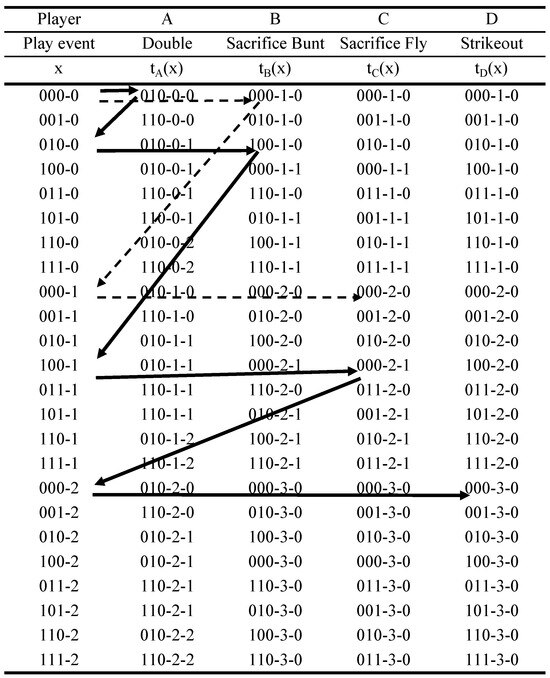
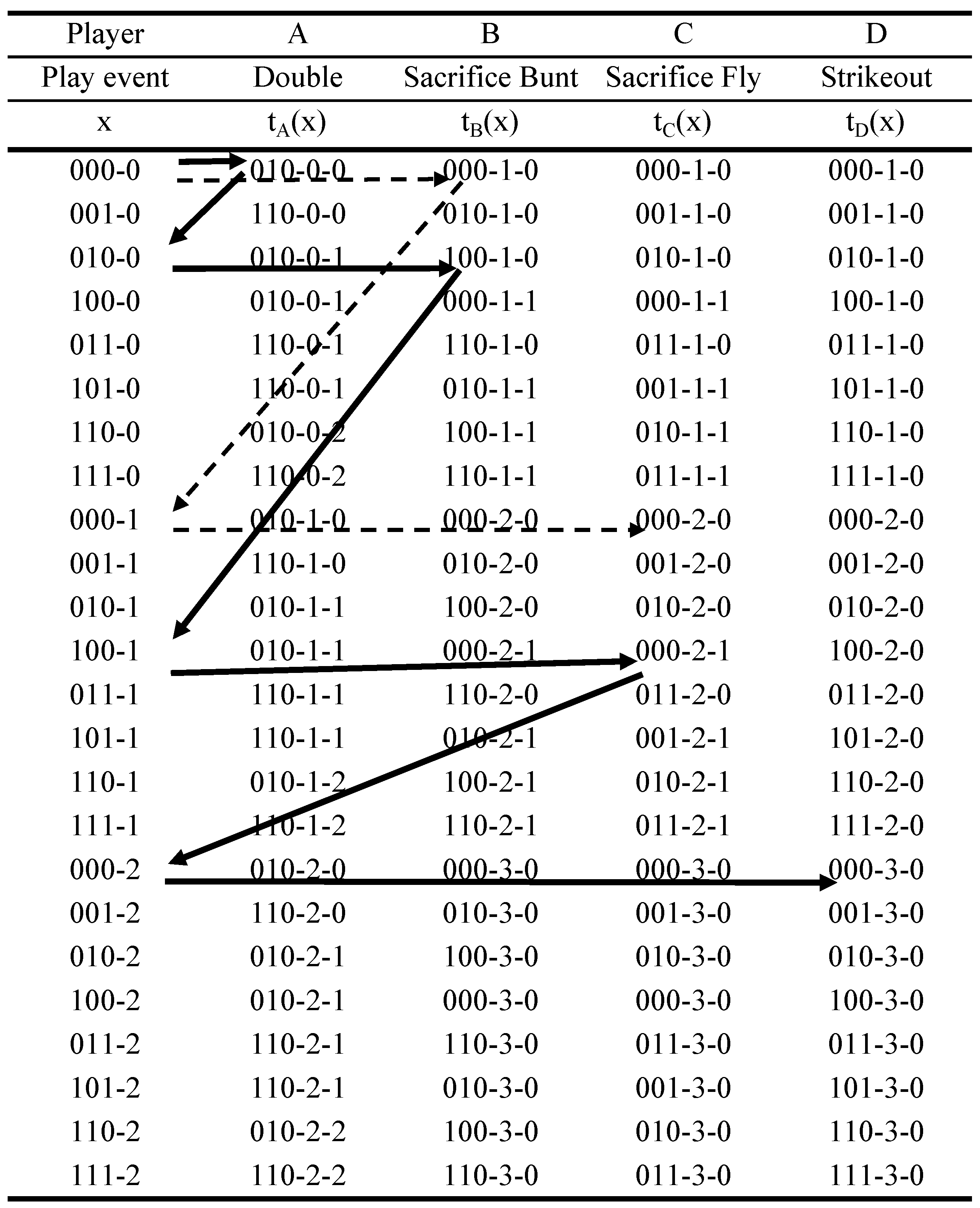
This is demonstrated in Figure 1 (from McBride, 2026). This inning has four actual plays: A’s double, B’s sacrifice bunt, C’s sacrifice fly, and D’s strikeout. Each play has a corresponding event trigger ($t_a$, $t_b$, $t_c$, and $t_d$, respectively) that maps from an initial state to a new base-out state and runs scored.

Figure 1. Example of event triggers for an inning. Notes: The solid arrows trace the path of the actual inning with all four players. The dotted arrows trace the hypothetical path of play for the hypothetical coalition of only players B and C.

The solid arrows trace the path of the actual inning. The inning began in initial state 000-0, and A’s double moved the game to state 010-0-0 (base-out state 010-0 with zero runs scored on the play). 010-0 is then the initial state for B’s sacrifice bunt, which changes the game to 100-1-0 (runner on third, one out, zero runs scored on the play). The next play begins in 100-1 and changes the game to 000-2-1 (based empty, two outs, and one run scored on the play). The final play results in the third out and no more runs scored. With one total run scored and three outs recorded, we set $R\left(S\right)=1$ and $O\left(S\right)=3$.

The dotted arrows trace out the course of play in the hypothetical coalition S that has only B and C’s event triggers. Whenever a subset of the plays is used, the relative order of the plays from the actual game is respected, so B’s trigger will occur first and C’s trigger second in this coalition. Any hypothetical coalition begins in initial state 000-0, and now B’s bunt moves the game to 000-1-0, after which C’s fly ball moves the game to 000-2-0. This hypothetical inning ends with 0 runs allowed and 2 outs recorded, i.e., $R\left(S\right)=0$ and $O\left(S\right)=2$.

With the basic mechanics of reconstructing hypothetical innings in place, McBride identified principles to follow when constructing event triggers. A vital one is actual state advancement: if a play event moved the actual game from initial state x to resulting state y with r runs scored on the play, then the event trigger for the play must also move the game to state to y with r runs scored when the initial state is x. This requirement is necessary to ensure that the values for the grand coalition are correct and the Shapley Values are efficient.

McBride next programmed a computer to construct event triggers for a large number of play events using Major League Baseball play-by-play data downloaded from www.Retrosheet.org, and then used the resulting event triggers to train machine learning models to create event triggers for all plays in all recorded Major League Baseball games for the 1916–2022 regular season and postseasons. Fortunately, I can use these event triggers in my calculations for SPR and SPO without having to create them again.

3.3. The Two-Stage Procedure to Calculate SPR and SPO

The second challenge is how to select which plays and event triggers to include when creating the value functions needed to calculate SPR and SPO for an inning. As will be explained below, McBride’s (2026) method for solving this second challenge cannot be used to credit pitchers. This section introduces a novel two-stage procedure for solving this challenge that yields fair measures of credit for pitchers.

For a given inning, let

$$I_P=\{pitche{r}_1,pitche{r}_2,\dots ,pitche{r}_k\},$$

(14)

denote the set of all pitchers in that inning, and further define $p_j\in I_P$ to be the pitcher associated with $pla{y}_j\in Plays$. By the rules of baseball, each $pla{y}_j$ must have a single baseball player in the pitcher role, so $p_j$ identifies just a single pitcher for $pla{y}_j$.

Because pitching and fielding are two distinct defensive roles, I impose a principle that I call pitcher anonymity:

The allocation of credit between pitchers and fielders does not depend on the identity of the pitcher.

This condition enforces a strict separation of the pitching and fielding roles and has two critical implications for the construction of value functions. The first implication is that the contributions of individual fielders do not need to be calculated separately, so that fielders can be depicted as a collective entity without the need to track which individual fielders were involved in each play. Let $f_j\in \{0,1\}$ take the value 1 if at least one fielder was involved in $pla{y}_j$ and take the value 0 otherwise. Fielding plays for which $f_j=1$ include plays with batted balls (ground-outs, fly-outs, etc.), but also plays like stolen bases, extra base advancements on wild pitches, and dropped-third strikes that involve or could have involved a fielder’s action. Note that a fielding play made by the pitcher has $f_j=1$ to keep the pitching and fielding roles separate. Non-fielding plays assigned $f_j=0$ include walks with standard base advances, strikeouts without base advances, home runs over the outfield fence, and hit by pitches.

We can now formally state that pitcher anonymity is satisfied if, holding $Plays$ and ${\left(f_j\right)}_{j=1}^m$ fixed, the total SPR and total SPO in an inning does not change if any element of $I_P$ or ${\left(p_j\right)}_{j=1}^m$ changes.

The second implication is that we must separate the Shapley Value calculation for an inning into a two-stage procedure. In the first stage, a Pitcher-Fielder Game is created for each of the possible coalitions of pitchers and the composite fielders. In the second stage, the Shapley Values from the first stage constitute the values in the value function in a single Between-Pitchers Game. The Shapley Values from this Between-Pitchers Game constitute the final SPR and SPO credit allocations. In effect, the first stage divides credit between pitchers and fielders while keeping pitching and fielding roles separate, while the second stage divides the pitchers’ total credit between the pitchers. If just a single stage is used, then pitcher anonymity cannot be ensured (discussed later).

3.3.1. Stage 1: The Pitcher–Fielder Games

Let $S\subseteq I_P$ be a coalition of pitchers for an inning. With k pitchers, there are $2^k$ such coalitions (i.e., the power set of coalitions). Each of these coalitions has its own Pitcher–Fielder Game, denoted $G_S$, which has two composite players: a composite actor $Pitcher{s}_S$ that treats all of the pitchers in S as if they are one pitcher, and a composite $Fielders$ actor that treats the fielders as one fielder. The set of players for the Pitcher–Fielder Game $G_S$ will thus always have two “actors”: $I_S=\{Pitcher{s}_S,Fielders\}$.

Because each Pitcher–Fielder Game has only two actors, there are four possible coalitions of these two actors: the $None$ coalition, the $Pitcher{s}_S$ coalition with only the composite actor of the pitchers in S, the $Fielders$ coalition with only the fielders, and the $All$ coalition with both $Pitcher{s}_S$ and $Fielders$.

Let $S^{\prime }\subseteq I_S$ be one of these coalitions. We use the event-trigger framework in Section 3.2 $G_S$ to construct the values for runs allowed $R^{\prime }\left(S\right)$ and outs recorded $O^{\prime }\left(R\right)$ for each $S^{\prime }\subseteq I_S$:

• The $S^{\prime }=None$ coalition has no associated plays, and sequencing through no event triggers yields $R^{\prime }\left(None\right)=0$ and $O^{\prime }\left(None\right)=0$.
• The $S^{\prime }=Pitcher{s}_S$ coalition includes only those plays for which $p_j\in S$ and $f_j=0$. Starting with $Plays$, remove any $pla{y}_j$ for which the associated pitcher $p_j$ is not in S and for which $f_j=1$, keeping the remaining plays in their respective order. Sequencing through these plays’ event triggers yields $R^{\prime }\left(Pitcher{s}_S\right)$ and $O^{\prime }\left(Pitcher{s}_S\right)$.
• The $S^{\prime }=Fielders$ coalition has no associated plays because each $pla{y}_j$ has an associated pitcher, so $R^{\prime }\left(Fielders\right)=0$ and $O^{\prime }\left(Fielders\right)=0$.
• The $S^{\prime }=All$ coalition includes all plays for which $p_j$ is in S, so remove any play for which $p_j$ is not in S. Sequencing through these plays’ event triggers yields $R^{\prime }\left(All\right)$ and $O^{\prime }\left(All\right)$.

With the value function now complete for $G_S$, we calculate the Shapley Values for $G_S$. Denote the Shapley Value for runs as $R\left(S\right)$, and the Shapley Value for outs as $O\left(S\right)$. Repeating this process of creating the Pitcher–Fielder Game and finding the Shapley Values for each coalition of pitchers $S\subseteq I_P$, we obtain $R\left(S\right)$ and $O\left(S\right)$ for every $S\subseteq I_P$.

This process is now demonstrated for the Two-Pitcher Inning example from Table 1. The set of pitchers is

$$I_P=\{A,B\},$$

(15)

and the set of possible pitcher coalitions is

$$\{\varnothing ,A,B,AB\}.$$

(16)

Each coalition S in this power set has its own Pitcher–Fielder Game, so there are four Pitcher–Fielder Games.

This Pitcher–Fielder Game for coalition $S=\varnothing$ is trivial because it does not have play events or event triggers, so the runs and outs Shapley Values for $G_{\varnothing }$ are $R(\varnothing )=0$ and $O(\varnothing )=0$.

The Pitcher–Fielder Game with all pitchers $S=AB$, denoted $G_{AB}$, is depicted in Table 3. Trivially, we must have $R^{\prime }\left(None\right)=0$ and $O^{\prime }\left(None\right)=0$, and also $R^{\prime }\left(Fielders\right)=0$ and $O^{\prime }\left(Fielders\right)=0$, as shown in panels (a) and (c) in the table, because the $None$ and $Fielders$ coalitions in $G_{AB}$ have no play events. The $Pitcher{s}_S$ coalition in panel (b) has three play events that involve only pitchers: the HR allowed by Pitcher A, the strikeout by Pitcher A, and the strikeout by Pitcher B, in that order. If these three play events occur in that order, then sequencing through their event triggers yields one run and two outs so that $R^{\prime }\left(Pitcher{s}_S\right)=1$ and $O^{\prime }\left(Pitcher{s}_S\right)=2$, as reported in the bottom-right of panel (b). Finally, the $All$ coalition in panel (d) includes event triggers for all play events in their actual order, so $R^{\prime }\left(All\right)=3$ and $O^{\prime }\left(All\right)=3$, as reported in the bottom-right of panel.

Table 3. Value function for the Pitcher–Fielder Game $G_{AB}$.

(a) Values for None Coalition
Play	Pitcher ${\mathit{p}}_{\mathit{j}}$	Fielding ${\mathit{f}}_{\mathit{j}}$	Runs	Outs
–	–	–	0	0
$R^{\prime }\left(None\right)=0$, $O^{\prime }\left(None\right)=0$
(b) Values for Pitchers Coalition
Play	Pitcher ${\mathit{p}}_{\mathit{j}}$	Fielding ${\mathit{f}}_{\mathit{j}}$	Runs	Outs
HR	A	0	1	0
K	A	0	0	1
K	B	0	0	1
$R^{\prime }\left(Pitcher{s}_S\right)=1$, $O^{\prime }\left(Pitcher{s}_S\right)=2$
(c) Values for Fielders Coalition
Play	Pitcher ${\mathit{p}}_{\mathit{j}}$	Fielding ${\mathit{f}}_{\mathit{j}}$	Runs	Outs
–	–	–	0	0
$R^{\prime }\left(Fielders\right)=0$, $O^{\prime }\left(Fielders\right)=0$
(d) Values for All Coalition
Play	Pitcher ${\mathit{p}}_{\mathit{j}}$	Fielding ${\mathit{f}}_{\mathit{j}}$	Runs	Outs
ROE	A	1	0	0
HR	A	0	2	0
K	A	0	0	1
DBL	A	1	0	0
DBL	B	1	1	0
K	B	0	0	1
GO	B	1	0	1
$R^{\prime }\left(All\right)=3$, $O^{\prime }\left(All\right)=3$

Table 4 completes the Shapley Value calculations for Pitcher–Fielder Game $G_{AB}$ using the value function information from Table 3. The Shapley Value is the average marginal value added to production in all possible orders that form the $All$ coalition. With just the two composite players, $Pitcher{s}_S$ and $Fielders$, there are only two orders: first, denoted $PF$, is to add $Pitcher{s}_S$ then $Fielders$; second, denoted $FP$, is to add $Fielders$ then $Pitcher{s}_S$. In order $PF$ in panel (a) of the table, the coalition before the pitchers are added (column $R^{\prime }\left(-P\right)$) is the $None$ coalition, and the coalition after they are added (column $R^{\prime }\left(+P\right)$) is just $Pitcher{s}_S$. The runs allowed values for these two coalitions are $R^{\prime }\left(None\right)=0$ and $R^{\prime }\left(Pitcher{s}_S\right)=1$, respectively, so the marginal increase in runs allowed (i.e., $m\left(P\right)$) from adding $Pitcher{s}_S$ to None is 1 as reported in in the right-most column. In the $FP$ order, the $Fielders$ are already in the coalition when the $Pitcher{s}_S$ are added. With $R^{\prime }\left(Fielders\right)=0$ and $R^{\prime }\left(All\right)=3$, the marginal increase in runs allowed when going from $Fielders$ to $All$ is 3. The average of these two marginal increases in runs allowed yields $R\left(AB\right)=(1+3)/2=2.00$, as displayed at the bottom of panel (a). A similar calculation for outs recorded in panel (b) yields $O\left(AB\right)=(2+3)/2=2.50$.

Table 4. Calculation of $R\left(AB\right)$ and $O\left(AB\right)$ for the Pitcher–Fielder Game $G_{AB}$.

(a) Calculation of $R\left(AB\right)$
	Coalition Before		Coalition After		$\mathit{m}\left(\mathit{P}\right)=$
Order	P Added	${\mathit{R}}^{\prime }(-\mathit{P})$	P Added	${\mathit{R}}^{\prime }(+\mathit{P})$	${\mathit{R}}^{\prime }(+\mathit{P})-{\mathit{R}}^{\prime }\left(\mathit{P}\right)$
$PF$	$None$	0	$Pitcher{s}_S$	1	1
$FP$	$Fielders$	0	$All$	3	3
$R\left(AB\right)=2.00$
(b) Calculation of $O\left(AB\right)$
	Coalition Before		Coalition After		$\mathit{m}\left(\mathit{P}\right)=$
Order	P Added	${\mathit{R}}^{\prime }(-\mathit{P})$	P Added	${\mathit{R}}^{\prime }(+\mathit{P})$	${\mathit{R}}^{\prime }(+\mathit{P})-{\mathit{R}}^{\prime }\left(\mathit{P}\right)$
$PF$	$None$	0	$Pitcher{s}_S$	2	2
$FP$	$Fielders$	0	$All$	3	3
$O\left(AB\right)=2.50$

There are two more Pitcher–Fielder Games: $G_A$ for the coalition of just Pitcher A and $G_B$ for the coalition of just Pitcher B. The value functions for these two games are provided in panels I and II, respectively, in Table 5. The logic used in these panels is identical to that as shown in Table 3 except for using only one pitcher. The Shapley Value calculations for the two games are in panels I and II of Table 6, where we see that $R\left(A\right)=1.50$ and $O\left(A\right)=1.00$ for Game $G_A$ and $R\left(B\right)=0.00$ and $O\left(B\right)=1.50$ for Game $G_B$. These calculations use the same logic as that used in Table 4.

Table 5. Value functions for Pitcher–Fielder Games $G_A$ and $G_B$.

I. Pitcher-Fielder Game ${\mathit{G}}_{\mathit{A}}$					II. Pitcher-Fielder Game ${\mathit{G}}_{\mathit{B}}$
(a) Values for $None$ Coalition					(a) Values for $None$ Coalition
Play	${\mathit{p}}_{\mathit{j}}$	${\mathit{f}}_{\mathit{j}}$	Runs	Outs	Play	${\mathit{p}}_{\mathit{j}}$	${\mathit{f}}_{\mathit{j}}$	Runs	Outs
–	–	–	0	0	–	–	–	0	0
$R^{\prime }\left(None\right)=0$, $O^{\prime }\left(None\right)=0$					$R^{\prime }\left(None\right)=0$, $O^{\prime }\left(None\right)=0$
(b) Values for $Pitcher{s}_S$ Coalition					(b) Values for $Pitcher{s}_S$ Coalition
Play	${\mathit{p}}_{\mathit{j}}$	${\mathit{f}}_{\mathit{j}}$	Runs	Outs	Play	${\mathit{p}}_{\mathit{j}}$	${\mathit{f}}_{\mathit{j}}$	Runs	Outs
HR	A	0	1	0	K	B	0	0	1
K	A	0	0	1
$R^{\prime }\left(Pitcher{s}_S\right)=1$, $O^{\prime }\left(Pitcher{s}_S\right)=1$					$R^{\prime }\left(Pitcher{s}_S\right)=0$, $O^{\prime }\left(Pitcher{s}_S\right)=1$
(c) Values for $Fielders$ Coalition					(c) Values for $Fielders$ Coalition
Play	${\mathit{p}}_{\mathit{j}}$	${\mathit{f}}_{\mathit{j}}$	Runs	Outs	Play	${\mathit{p}}_{\mathit{j}}$	${\mathit{f}}_{\mathit{j}}$	Runs	Outs
–	–	–	0	0	–	–	–	0	0
$R^{\prime }\left(Fielders\right)=0$, $O^{\prime }\left(Fielders\right)=0$					$R^{\prime }\left(Fielders\right)=0$, $O^{\prime }\left(Fielders\right)=0$
(d) Values for $All$ Coalition					(d) Values for $All$ Coalition
Play	${\mathit{p}}_{\mathit{j}}$	${\mathit{f}}_{\mathit{j}}$	Runs	Outs	Play	${\mathit{p}}_{\mathit{j}}$	${\mathit{f}}_{\mathit{j}}$	Runs	Outs
ROE	A	1	0	0	DBL	B	1	0	0
HR	A	0	2	0	K	B	0	0	1
K	A	0	0	1	GO	B	1	0	1
DBL	A	1	0	0
$R^{\prime }\left(All\right)=2$, $O^{\prime }\left(All\right)=1$					$R^{\prime }\left(All\right)=0$, $O^{\prime }\left(All\right)=2$

Table 6. Shapley Value calculations for Pitcher–Fielder Games $G_A$ and $G_B$.

I. Pitcher-Fielder Game ${\mathit{G}}_{\mathit{A}}$				II. Pitcher-Fielder Game ${\mathit{G}}_{\mathit{B}}$
(a) Calculation of $R\left(AB\right)$				(a) Calculation of $R\left(AB\right)$
Order	${\mathit{R}}^{\prime }(-\mathit{P})$	${\mathit{R}}^{\prime }(+\mathit{P})$	$\mathit{m}\left(\mathit{P}\right)$	Order	${\mathit{R}}^{\prime }(-\mathit{P})$	${\mathit{R}}^{\prime }(+\mathit{P})$	$\mathit{m}\left(\mathit{P}\right)$
$PF$	0	1	1	$PF$	0	0	0
$FP$	0	2	2	$FP$	0	0	0
$R\left(A\right)=1.50$				$R\left(B\right)=0.00$
(b) Calculation of $O\left(AB\right)$				(b) Calculation of $O\left(AB\right)$
Order	${\mathit{R}}^{\prime }(-\mathit{P})$	${\mathit{R}}^{\prime }(+\mathit{P})$	$\mathit{m}\left(\mathit{P}\right)$	Order	${\mathit{R}}^{\prime }(-\mathit{P})$	${\mathit{R}}^{\prime }(+\mathit{P})$	$\mathit{m}\left(\mathit{P}\right)$
$PF$	0	1	1	$PF$	0	1	1
$FP$	0	1	1	$FP$	0	2	2
$O\left(A\right)=1.00$				$O\left(B\right)=1.50$

With these Shapley Values calculated, we can now move to the Between-Pitchers Game to calculate SPR and SPO for each pitcher.

3.3.2. Stage 2: The Between-Pitchers Game

There is only one Between-Pitchers Game for an inning. Its set of players is $I_P$, and for coalition $S\in I_P$, the values $R\left(S\right)$ and $O\left(S\right)$ are exactly the $R\left(S\right)$ and $O\left(S\right)$ Shapley Values from the Pitcher–Fielder Game $G_S$. The Shapley Values of this Between-Pitchers Game are then the final SPR and SPO values for the inning.

Table 7 provides the analysis of the Between-Pitchers Game for the Two-Pitcher Inning, with the calculation for SPR in panel I on the left and the calculation for SPO in panel II on the right. Observe that $R\left(S\right)$ and $O\left(S\right)$ for the value function for each S, shown in panels I(a) and II(a) for runs allowed and outs recorded, respectively, are the $R\left(S\right)$ and $O\left(S\right)$ Shapley Values from Pitcher–Fielder Game $G_S$. For example, values $R\left(A\right)$ and $R\left(B\right)$ are the taken from Table 6, and $R\left(AB\right)$ is from Table 4. Finally, notice that the SPR and SPO Shapley Values at the bottom of panels I(b), I(c), II(b), and II(c) are exactly the Shapley Values first shown in Table 2. Thus, we have completed the two-stage procedure to calculate SPR and SPO.

Table 7. Between-Pitchers Games for the Two-Pitcher Inning.

I. SPR				II. SPO
(a) Value Function				(a) Value Function
$R\left(None\right)$			$0.00$	$O\left(None\right)$			$0.00$
$R\left(A\right)$			$1.50$	$O\left(A\right)$			$1.00$
$R\left(B\right)$			$0.00$	$O\left(B\right)$			$1.50$
$R\left(AB\right)$			$2.00$	$O\left(AB\right)$			$2.50$
(b) SPR Calculation for Pitcher A				(b) SPO Calculation for Pitcher A
Order	$\mathit{R}(-\mathit{A})$	$\mathit{R}(+\mathit{A})$	$\mathit{m}\left(\mathit{A}\right)$	Order	$\mathit{R}(-\mathit{A})$	$\mathit{R}(+\mathit{A})$	$\mathit{m}\left(\mathit{A}\right)$
$AB$	0	1.50	1.50	$AB$	0	1.00	1.00
$BA$	0	2.00	2.00	$BA$	1.50	2.50	1.00
$SPRA=1.75$				$SPOA=1.00$
(c) SPR Calculation for Pitcher B				(c) SPO Calculation for Pitcher B
Order	$\mathit{R}(-\mathit{B})$	$\mathit{R}(+\mathit{B})$	$\mathit{m}\left(\mathit{B}\right)$	Order	$\mathit{R}(-\mathit{B})$	$\mathit{R}(+\mathit{B})$	$\mathit{m}\left(\mathit{B}\right)$
$AB$	1.50	2.00	0.50	$AB$	1.00	2.50	1.50
$BA$	0	0	0	$BA$	0	1.50	1.50
$SPRB=0.25$				$SPOB=1.50$

3.4. Key Features

Several features of the SPR and SPO calculations are worth noting. First, the two-stage procedure described in Section 3.3 distinguishes the calculation of SPR and SPO from the calculation of the offensive Shapley baseball statistics in McBride (2026). The offensive Shapley statistics are calculated in a single stage because there is no division of roles in baseball offense like that between pitching and fielding on defense. However, if a single-stage method was used to calculate SPR and SPO using the set of players,

$$I=\{pitche{r}_1,pitche{r}_2,\dots ,pitche{r}_k,Fielders\},$$

(17)

then the Shapley Values would violate pitcher anonymity. For example, in the Two-Pitchers Example, a single-stage approach yields $1.83$ SPR for A and $0.33$ SPR for B, which totals $2.17$ SPR for the pitchers combined. But, if there was only one pitcher, then the total SPR would be $2.00$, thus violating pitcher anonymity. Pitcher anonymity is only maintained using the two-stage procedure.

Second, when there are multiple pitchers in an inning, the Pitcher–Fielder Game for the full set of pitchers ($S=I_P$) actually provides a clean division of total credit between the combined collection of pitchers and the combined collection of fielders. For example, the $R\left(AB\right)=2.00$ and $O\left(AB\right)=2.50$ Shapley Values in Table 4 are exactly the total SPR and total SPO shown in Table 2. The fielders’ collective share of credit for runs and outs is then easily calculated as the total runs and outs in the inning minus the pitchers’ SPR and SPO.

Third, the frequent equal splitting of credit between pitchers and fielders or between different pitchers is neither accidental nor intentional; it follows from the value functions and the Shapley Value formula (Equation (7)) combined with the pitcher-anonymity assumption. Because all members of a coalition must have participated in the play for it to be included in that coalition’s play events, the marginal increase in runs allowed (or outs made) when adding a pitcher to a fielder or adding the fielder to the pitcher will be the same for play events in which both participated. By the symmetry feature of the Shapley Value, the pitcher and fielder will be given equal credit for such plays. Thus, pitchers and fielders will split the credit in half for runners who reached base or scored via balls in play, as well as for outs on balls in play. Equally splitting SPR between pitchers is also standard for runners who reached base against one pitcher but scored against another pitcher.

Fourth, in contrast to earned runs, SPR does not make a distinction between plays with fielding errors and those without errors because the pitcher and fielders share credit (blame) for the outcomes of balls in play whether or not an error occurred. SPR assumes that pitchers and fielders work together to make outs, and when an out is missed on a ball in play for whatever reason, then the blame is shared. Standard scorekeeping places the full blame on the fielder for a throwing error or a dropped ball, but the pitcher allowed the ball to be put in play. With better pitching, the batter would not have put the ball in play, so the pitcher deserves some credit (blame) for the play. This may seem unfair to the pitcher from the point of view of the standard scorekeeping used to calculate earned runs, but it is consistent with the coalitional representation of run prevention in baseball. Note also that ignoring whether a fielder error occurred in the SPR and SPO calculations relieves the scorekeeper of having to use their individual judgment about whether an error occurs, which is often subjective, inconsistently determined, and prone to home-team bias.

Fifth, despite the non-triviality in their calculation, SPR and SPO are easy to interpret and use. SPR and SPO are merely shares of credit, making them easy to understand, even if their calculation is complex. Indeed, most advancements in baseball statistics involve replacing inferior but simpler statistics with newer but more complex statistics that the layperson can use even though they are unable to calculate them on their own. SPR and SPO follow this same trend. Moreover, by the Shapley Value’s additivity property, SPR and SPO are simply added across all of the innings in a game to get the SPR and SPO for a game, or added across all innings in a series or season to get SPR and SPO for a series or season, respectively. Because SPR and SPO are constructed and calculated inning by inning, any aggregation over multiple innings is done simply by adding the SPR or SPO from those individual innings.

Finally, official scorekeepers can be trained to assign event triggers to plays as part of their real-time responsibilities. This would enable the calculation of SPR and SPO at the end of each inning and make them available for inclusion in a box score at the end of the game.

3.5. Calculating Hypothetical Runs and Outs for Past MLB Games

I calculated SPR and SPO for the 2022 Major League Baseball regular season and the 1955–2022 World Series. I began with the machine learning event triggers created by McBride (2026) using Retrosheet.org play-by-play data. I then reprocessed the data from Retrosheet.org to identify for each $pla{y}_j$ and its associated event trigger the pitcher of record ($p_j$) and whether or not the play involved fielders ($f_j$). These pitching and fielding identifications were then merged with the machine learning event triggers. Finally, taking one inning at a time, each pitcher’s SPR and SPO was calculated via the two-stage procedure. Shapley Values were calculated using the Arrar–Declos Shapley Value algorithm (Araar & Duclos, 2009).

4. Results

4.1. Result 1: Standard Pitcher Credit Statistics Miscredit Runs and Outs by 40–50%

I use SPR and SPO for the 2022 MLB regular season to examine how earned runs (ER), runs allowed (R), and innings pitched (IP) miscredit pitchers. The 189,073 plays yielded 48,661 inning-level SPR and SPO calculations that could be summed together for analysis. The first column in Table 8 reports the MLB totals for SPR, SPO, ER, R, IP, and OUTS for the 2022 season. OUTS, which is $3\times IP$, is provided for easier comparison with SPO.

Table 8. Quantification of miscredit, 2022 MLB regular season.

		MLB	Starting Pitchers	Relief Pitchers
Statistic	MLB	(min 50 IP)	(min 50 IP)	(min 50 IP)
SPR	13,675.50	10,033.54	5675.46	4358.08
SPO	84,810.50	66,711.33	38,122.58	28,588.75
ER	18,993	14,055	8215	5840
R	20,817	15,417	8851	6566
IP	43,075.1	33,827.0	19,539.1	14,287.2
OUTS	129,226	101,481	58,618	42,863
ER/SPR	1.39	1.40	1.45	1.34
R/SPR	1.52	1.54	1.56	1.51
OUTS/SPO	1.52	1.52	1.54	1.50

Notes: SPR and SPO are from the author’s calculations. OUTS $=3\times$ IP. ER, R, and IP are from https://www.fangraphs.com/ (accessed on 1 November 2024). 0.1 IP denotes one-third of an inning pitched, and 0.2 denotes two-thirds of an inning pitched.

The three bottom rows provide the measures of miscredit. ER divided by SPR (ER/SPR) is an intuitive measure of miscredit. The more ER/SPR is above 1, the greater the amount that the ER statistic overcredits for runs that score. Having ER/SPR equal to $1.39$ means that the ER statistic overcredited the 2022 MLB pitchers for runs that scored by $39\%$. Because ER is always less than R, the R statistic must overcredit pitchers by a larger amount than ER, in this case $52\%$ as measured by R/SPR. OUTS/SPO indicates that OUTS (and IP by extension) overcredited pitchers by $52\%$. The second column reports very similar calculations when including only the pitchers with at least 50 IP in the 2022 MLB regular seasons, indicating that the overcrediting by ER, R, and IP is not significantly altered by pitchers who rarely pitched. That the overcrediting is so large provides an empirical justification for the motivation to create better credit measures of pitching performance.

4.2. Result 2: Starting Pitchers Are Overcredited by a Larger Amount than Relief Pitchers

The last two columns in Table 8 separate the miscredit measures for starting pitchers and relief pitchers (minimum 50 IP). I classify a pitcher as a starting pitcher if they started at least $90\%$ of their game appearances. Applying this threshold results in $58\%$ of the IP in this sample being attributed to starting pitchers, which is very close to the $59\%$ of IP that https://www.fangraphs.com/ attributes to starting pitchers in the full sample.

We see that the overcrediting of runs to pitchers differs significantly between starting pitchers and relief pitchers, with starting pitchers being overcredited for runs by $45\%$ compared to only $34\%$ for relief pitchers. This result confirms the claim made earlier in the paper that starting pitchers are consistently and unfairly given too much blame in the ER statistic for runners they allowed to reach base but who scored when another pitcher was pitching. SPR avoids this unfair allotment of credit.

Starting pitchers are also overcredited more for outs than relief pitchers as measured by OUTS/SPO, but the difference between starting pitchers and relief pitchers is only $4\%$. This difference is due in part to the fact that relief pitchers unfairly receive more credit for outs in the IP (OUTS) statistic, as mentioned earlier. However, some of the difference may be due to different pitching styles between starting pitchers and relief pitchers. In particular, relief pitchers strike out more batters per IP than starting pitchers ($9.06$ vs. $8.33$ K/9 in the 2022 MLB regular season), and this means that relief pitchers will deserve a higher share of credit for team outs than starting pitchers.

4.3. Result 3: SRA Ranks Pitchers Differently than ERA and FIP

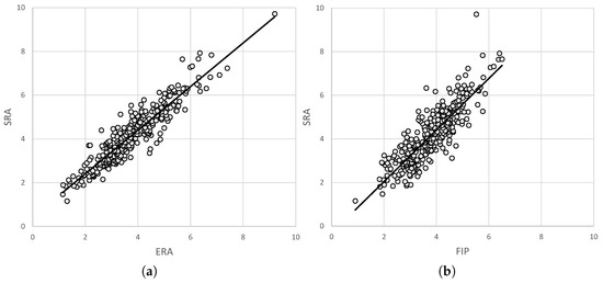
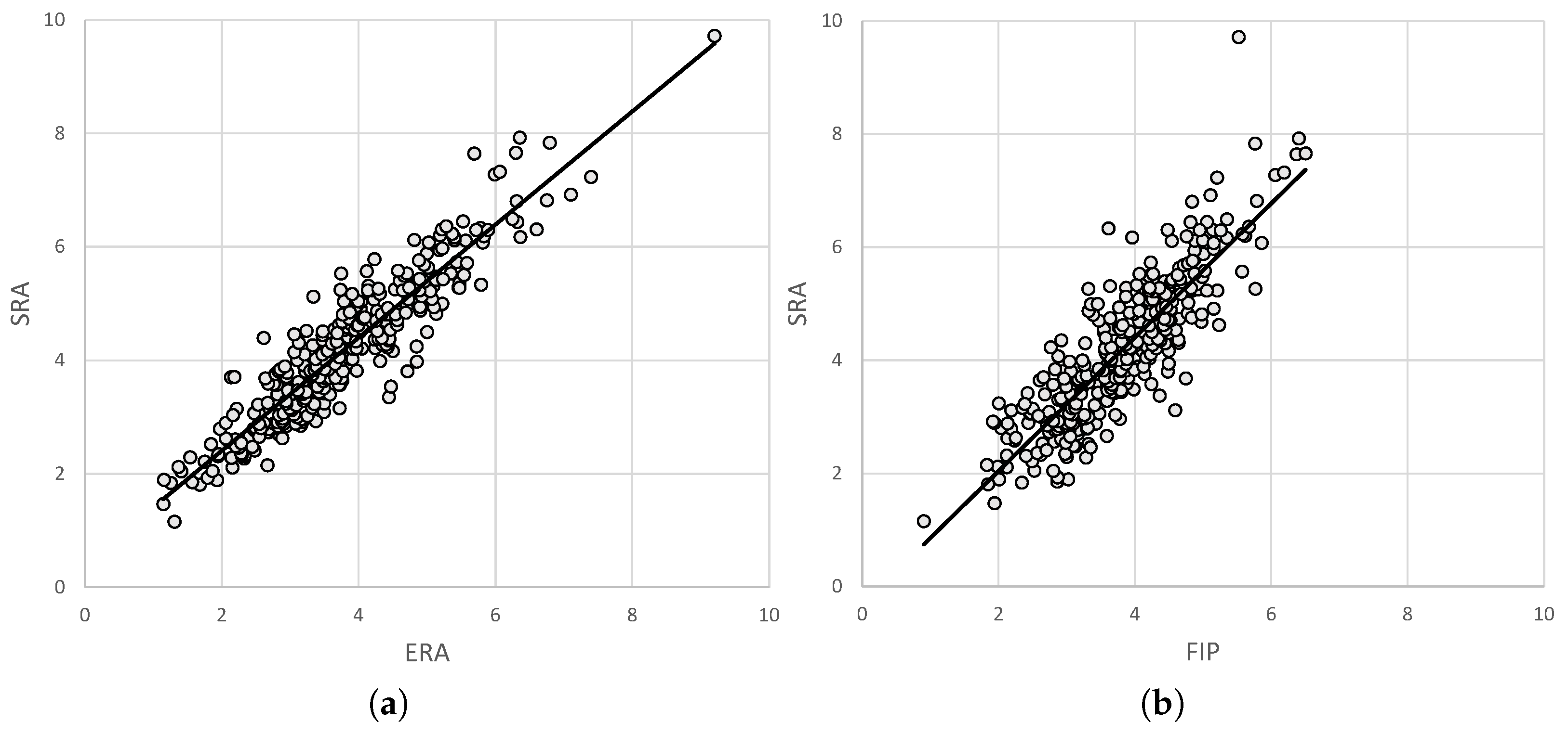
The two graphs in Figure 2 illustrate how SRA compares with the earned-run average (ERA) and fielding-independent pitching (FIP) for the 2022 MLB regular season (minimum 50 IP). In Figure 2a, each dot represents the SRA and ERA for a different pitcher, and the solid line represents the best linear fit. We find a clear and strong correlation of $0.93$ between SRA and ERA. The correlation between SRA and FIP is slightly lower at $0.86$, which matches the larger spread in Figure 2b. For comparison, the correlation between ERA and FIP in this sample is even lower at $0.75$.

Figure 2. SRA with ERA and FIP for 2022 MLB regular season pitchers, minimum 50 IP. ERA and FIP obtained from https://www.fangraphs.com/ (accessed on 1 November 2024). (a) plots SRA and ERA with best linear fit. (b) plots SRA and FIP with best linear fit.

That the correlation between ERA and FIP is the lowest of the three is instructive. By not counting fielded balls in play, FIP can be understood as a correction to ERA that estimates what a pitcher’s ERA should be with average fielder quality and batted-ball luck. Meanwhile, SRA provides a different kind of correction to ERA. Like FIP, SRA credits pitchers differently based on whether the play could be fielded, but like ERA, SRA still assigns some credit to pitchers for all balls in play. So SRA combines key features of both ERA and FIP, and this likely explains why SRA is more strongly correlated with ERA and FIP than ERA and FIP are to each other.

This same logic also explains why, if a pitcher’s FIP is higher (lower) than their ERA, their SRA also tends to be higher (lower) than their ERA. Of the pitchers in this sample, $53\%$ have SRA and FIP higher than ERA, and $14\%$ have SRA and FIP lower than ERA. Thus, for $67\%$ of the pitchers, SRA and FIP provide a directionally similar correction to ERA, but with SRA making a smaller correction than FIP.

Recall that SRA is strictly pitcher-only, while ERA and FIP are not. ERA’s numerator (ER) and denominator (IP) reflect team performance when a pitcher pitched, and while FIP’s numerator reflects the pitcher’s individual performance, its dominator (IP) does not. In contrast, SRA uses pitcher-only measures in its numerator and denominator. As a consequence, SRA ranks pitchers differently than ERA and FIP, as seen in Table 9 which lists the 25 most efficient pitchers in the 2022 MLB regular season, as measured by SRA (minimum 50 IP). According to SRA, the most efficient pitcher in 2022 was the relief pitcher Edwin Diaz, who was also 1st in FIP and 4th in ERA. In fact, the top 13 pitchers by SRA were relief pitchers, which matches the conventional wisdom that relief pitchers are selected in part for strikeout ability. That said, several starting pitchers also appear on the leaderboard, including Justin Verlander (14th), Shohei Ohtani (18th), and Clayton Kershaw (22nd).

Table 9. Top 25 efficient pitchers, 2022 MLB regular season, minimum 50 IP.

	SP/						ER/	R/	OUTS/	SRA/	ERA/	FIP/
Name	RP	SPR	SPO	SRA	ERA	FIP	SPR	SPR	SPO	Rank	Rank	Rank
E Diaz	RP	6.50	152.00	1.15	1.31	0.90	1.38	1.38	1.22	1	4	1
E Phillips	RP	7.25	133.25	1.47	1.14	1.94	1.10	1.52	1.42	2	1	6
E Swanson	RP	7.71	115.25	1.81	1.68	1.85	1.30	1.43	1.40	3	9	3
R Helsley	RP	9.75	143.25	1.84	1.25	2.34	0.92	1.13	1.35	4	3	19
J Adam	RP	9.00	131.00	1.86	1.56	2.86	1.22	1.33	1.45	5	8	52
D Williams	RP	9.75	139.25	1.89	1.93	2.01	1.33	1.74	1.31	6	14	9
R Stanek	RP	7.83	111.75	1.89	1.15	3.02	0.89	1.02	1.47	7	2	71
D Bard	RP	9.00	126.00	1.93	1.79	2.86	1.33	1.67	1.44	8	11	53
C Perez	RP	8.67	114.50	2.04	1.40	2.80	1.04	1.27	1.51	9	6	46
J Duran	RP	11.00	145.00	2.05	1.86	2.52	1.27	1.36	1.40	10	13	30
A Vesia	RP	9.50	121.50	2.11	2.15	2.12	1.37	1.47	1.34	11	23	12
E Clase	RP	11.50	146.50	2.12	1.36	1.98	0.96	1.57	1.49	12	5	7
S Strider	RP	23.75	298.25	2.15	2.67	1.83	1.64	1.77	1.32	13	56	2
J Verlander	SP	29.00	353.50	2.22	1.75	2.49	1.17	1.48	1.49	14	10	28
S Hentges	RP	10.83	128.75	2.27	2.32	2.48	1.48	1.57	1.44	15	34	27
T Gonsolin	SP	21.50	254.50	2.28	2.14	3.28	1.44	1.49	1.54	16	22	104
A Bass	RP	12.00	141.58	2.29	1.54	3.00	1.00	1.25	1.49	17	7	69
S Ohtani	SP	30.50	356.25	2.31	2.33	2.40	1.41	1.48	1.40	18	35	22
B Abreu	RP	11.50	134.25	2.31	1.94	2.12	1.13	1.39	1.35	19	15	11
M Scherzer	SP	26.25	304.50	2.33	2.29	2.62	1.41	1.49	1.43	20	32	34
M Moore	RP	13.25	152.50	2.35	1.95	2.98	1.21	1.51	1.46	21	16	64
C Kershaw	SP	22.50	257.25	2.36	2.28	2.57	1.42	1.60	1.47	22	30	31
M Fried	SP	32.25	361.00	2.41	2.48	2.70	1.58	1.71	1.54	23	41	39
A Manoah	SP	35.00	384.00	2.46	2.24	3.35	1.40	1.57	1.54	24	29	114
N Cortes	SP	29.25	319.25	2.47	2.44	3.13	1.47	1.50	1.49	25	38	88

Notes: SP = starting pitcher; RP = relief pitcher. ERA and FIP are from https://www.fangraphs.com/ (accessed on 1 November 2024). All other statistics are from the author’s calculations.

Despite the correlation between the pitchers’ SRA rank, ERA rank and FIP rank seen in Table 9, there are notable differences. For example, Max Fried is 16 positions higher in SRA ranking than in FIP ranking, and 18 positions higher than in the ERA ranking. His pitching efficiency is particularly underappreciated by ERA and FIP. His ER/SPR of $1.58$ is the highest among all pitchers in Table 9, making him the most overcredited (i.e., overblamed) pitcher on this list. Also notable is Nestor Cortes, whose SRA ranking is 13 positions higher than his ERA ranking and 53 spots higher than his FIP ranking. With an ER/SPR of $1.47$, he was overcredited the third most on this list. When accounting only for shares of runs and outs for which they deserve credit, Fried and Cortes were much more efficient than what standard statistics say.

Not shown in Table 9 are some other pitching performances of note. Relief pitcher Matt Brash ($50.2$ IP, $3.35$ SRA) had the highest ER/SPR of $1.91$ among all pitchers in this sample. The ER statistic unfairly blames him for almost twice as many runs as SPR. He ranks 97th in SRA, but ranks 129th in FIP and 257th in ERA, making him one of the most underappreciated pitchers according to the standard stats. Three other relief pitchers had ER/SPR over $1.80$: Brayan Bello ($1.88$), Joely Rodriguez ($1.84$), and Nick Nelson ($1.83$). The most overcredited starting pitcher according to ER/SPR was Ian Anderson ($1.72$).

There are also some pitchers who rate worse according to SRA than ERA and FIP. Six of the 347 pitchers in the sample had larger SPR than ER so that their ER/SPR was less than 1: Jaime Barria ($0.96$), Emmanual Clase ($0.96$), Ryan Helsley ($0.92$), Ryne Stanek ($0.89$), Scott Barlow ($0.88$), and Dylan Lee ($0.83$). These relief pitchers had a high fraction of unearned runs allowed for which SRA does not fully absolve them of blame. The standard stats do not blame these pitchers enough.

4.4. Result 4: SRA Identifies Efficient World Series Pitcher Performances

The World Series is the best-of-seven series played between two teams that determines the champion of Major League Baseball for a season. Between 1955, the first year in which a World Series MVP was selected, and 2022, there have been 29 pitchers selected as World Series MVP. These 29 pitchers and several of their statistics from their respective World Series are listed chronologically in Table 10. That these pitchers won the MVP award for their performances signals that their performances were recognized as critical to their team’s success in the World Series. But when comparing this list with Table 11, which lists the top pitcher performances by SRA (minimum 20 SPR and maximum $1.50$ SRA), we see that there are many impressive World Series performances that did not result in an MVP selection.

Table 10. Pitcher World Series Most Valuable Players, 1955–2022.

Year	Pitcher	W-L-S	IP	R	ER	HR	K	ERA	FIP	SPR	SPO	SRA
1955	J Podres (BRO)	2-0-0	18.0	3	2	1	10	1.00	2.65	2.00	32.00	1.69
1956	D Larsen (NYY)	1-0-0	10.2	4	0	0	7	0.00	2.18	1.92	17.00	3.05
1957	L Burdette (MLN)	3-0-0	27.0	2	2	1	13	0.67	2.42	1.50	47.00	0.86
1958	B Turley (NYY)	2-1-1	16.1	5	5	2	13	2.76	3.76	3.25	31.00	2.83
1959	L Sherry (LAD)	2-0-2	12.2	1	1	0	5	0.71	2.46	0.75	21.50	0.94
1961	W Ford (NYY)	2-0-0	14.0	0	0	0	7	0.00	2.00	0.00	24.50	0.00
1962	R Terry (NYY)	2-1-0	25.0	5	5	2	16	1.80	2.67	3.50	45.50	2.08
1963	S Koufax (LAD)	2-0-0	18.0	3	3	2	23	1.50	1.87	2.50	38.50	1.75
1964	B Gibson (STL)	2-1-0	27.0	11	9	4	31	3.00	3.35	7.50	55.50	3.65
1965	S Koufax (LAD)	2-1-0	24.0	2	1	0	29	0.38	0.73	1.00	50.50	0.53
1967	B Gibson (STL)	3-0-0	27.0	3	3	1	26	1.00	1.65	2.00	53.50	1.01
1968	M Lolich (DET)	3-0-0	27.0	5	5	2	21	1.67	2.57	3.50	51.00	1.85
1974	R Fingers (OAK)	1-0-2	9.1	2	2	2	6	1.93	5.04	2.00	17.00	3.18
1985	B Saberhagen (KCR)	2-0-0	18.0	1	1	0	10	0.50	1.74	0.50	32.00	0.42
1987	F Viola (MIN)	2-1-0	19.1	8	8	1	16	3.72	2.35	5.00	37.00	3.65
1988	O Hershiser (LAD)	2-0-0	18.0	2	2	0	17	1.00	0.92	1.00	35.50	0.76
1989	D Stewart (OAK)	2-0-0	16.0	3	3	1	14	1.69	2.20	2.00	31.00	1.74
1990	J Rijo (CIN)	2-0-0	15.1	1	1	0	15	0.59	1.83	0.50	30.00	0.45
1991	J Morris (MIN)	2-0-0	23.0	3	3	1	15	1.17	3.29	1.67	42.25	1.07
1995	T Glavine (ATL)	2-0-0	14.0	2	2	1	11	1.29	3.75	1.50	26.50	1.53
1996	J Wetteland (NYY)	0-0-4	4.1	1	1	0	6	2.08	1.10	0.50	9.50	1.42
1997	L Hernandez (FLA)	2-0-0	13.2	9	8	3	7	5.27	7.13	6.50	24.00	7.31
1999	M Rivera (NYY)	1-0-2	4.2	0	0	0	3	0.00	2.49	0.00	8.50	0.00
2001	R Johnson (ARI)	3-0-0	17.1	2	2	0	19	1.04	1.38	1.00	35.50	0.76
2001	C Schilling (ARI)	1-0-0	21.1	4	4	2	26	1.69	2.25	3.00	45.00	1.80
2003	J Beckett (FLA)	1-1-0	16.1	2	2	0	19	1.10	1.81	0.75	34.00	0.60
2008	C Hamels (PHI)	1-0-0	13.0	4	4	1	8	2.77	3.59	2.50	23.50	2.87
2014	M Bumgarner (SFG)	2-0-1	21.0	1	1	1	17	0.43	2.42	1.00	40.00	0.68
2019	S Strasburg (WAS)	2-0-0	14.1	4	4	2	14	2.51	3.70	3.00	28.50	2.84

Notes: SPR, SPO, and SRA are from the author’s calculations. ERA, IP, and other statistics are from BaseballReference.com (accessed on 1 November 2024). FIP is calculated using yearly FIP constants from https://www.fangraphs.com/ (accessed on 1 November 2024). W-L-S = wins–losses–saves, IP = innings pitched, R = runs allowed, ER = earned runs allowed, HR = home runs, K = strikeouts. 0.1 IP denotes one-third of an inning pitched and 0.2 denotes two-thirds. Johnson and Schilling were co-MVPs in 2001.

Table 11. World Series pitchers with SPO $\ge 20$ and SRA $\le 1.5$, 1955–2022.

Year	Pitcher	W-L-S	IP	R	ER	HR	K	ERA	FIP	SPR	SPO	SRA
1960 *	W Ford (NYY)	2-0-0	18.0	0	0	0	8	0.00	1.97	0.00	31.00	0.00
1961	W Ford (NYY)	2-0-0	14.0	0	0	0	7	0.00	2.00	0.00	24.50	0.00
1985	B Saberhagen (KCR)	2-0-0	18.0	1	1	0	10	0.50	1.74	0.50	32.00	0.42
1990	J Rijo (CIN)	2-0-0	15.1	1	1	0	15	0.59	1.83	0.50	30.00	0.45
1972 *	J Billingham (CIN)	1-0-1	13.2	1	0	0	11	0.00	1.67	0.50	25.75	0.52
1965	S Koufax (LAD)	2-1-0	24.0	2	1	0	29	0.38	0.73	1.00	50.50	0.53
1956 **	B Turley (NYY)	0-1-0	11.0	1	1	0	14	0.82	2.01	0.50	23.50	0.57
2003	J Beckett (FLA)	1-1-0	16.1	2	2	0	19	1.10	1.81	0.75	34.00	0.60
1956 **	C Labine (BRO)	1-0-0	12.0	1	0	0	7	0.00	1.95	0.50	21.50	0.63
2014	M Bumgarner (SFG)	2-0-1	21.0	1	1	1	17	0.43	2.42	1.00	40.00	0.68
1988	O Hershiser (LAD)	2-0-0	18.0	2	2	0	17	1.00	0.92	1.00	35.50	0.76
2001	R Johnson (ARI)	3-0-0	17.1	2	2	0	19	1.04	1.38	1.00	35.50	0.76
1957	L Burdette (MLN)	3-0-0	27.0	2	2	1	13	0.67	2.42	1.50	47.00	0.86
1972 *	BM Odom (OAK)	0-1-0	11.1	2	2	0	13	1.59	1.69	0.75	23.50	0.86
2013 *	J Lester (BOS)	2-0-0	15.1	1	1	1	15	0.59	2.13	1.00	30.50	0.89
2001 **	R Clemens (NYY)	1-0-0	13.1	2	2	0	19	1.35	1.32	1.00	29.75	0.91
1959	L Sherry (LAD)	2-0-2	12.2	1	1	0	5	0.71	2.46	0.75	21.50	0.94
2017 **	C Morton (HOU)	1-0-0	10.1	2	2	0	11	1.74	1.61	0.75	21.00	0.96
1957 **	W Ford (NYY)	1-1-0	16.0	2	2	0	7	1.13	2.52	1.00	27.50	0.98
1985 **	D Cox (STL)	0-0-0	14.0	2	2	0	13	1.29	1.68	1.00	27.50	0.98
1967	B Gibson (STL)	3-0-0	27.0	3	3	1	26	1.00	1.65	2.00	53.50	1.01
1991	J Morris (MIN)	2-0-0	23.0	3	3	1	15	1.17	3.29	1.67	42.25	1.07
1981 *	T John (NYY)	1-0-0	13.0	1	1	0	8	0.69	1.37	1.00	23.50	1.15
1971 *	S Blass (PIT)	2-0-0	18.0	2	2	1	13	1.00	2.40	1.50	33.50	1.21
2022 *	F Valdez (HOU)	2-0-0	12.1	2	2	1	18	1.46	2.71	1.25	27.50	1.23
2003 **	A Pettitte (NYY)	1-1-0	15.2	3	1	0	14	0.57	2.01	1.50	30.50	1.33
1985 **	D Jackson (KCR)	1-1-0	16.0	3	3	0	12	1.69	2.12	1.50	30.00	1.35
1997 **	C Ogea (BAL)	2-0-0	11.2	2	2	0	5	1.54	3.28	1.00	20.00	1.35
1968 **	B Gibson (STL)	2-1-0	27.0	5	5	1	35	1.67	0.72	3.00	58.00	1.40
1972 *	R Fingers (OAK)	1-1-2	10.1	2	2	0	11	1.74	1.72	1.17	21.00	1.50

Notes: SPR, SPO, and SRA from author’s calculations. All other statistics except FIP are from BaseballReference.com (accessed on 1 November 2024). FIP is calculated by the author using yearly FIP constants from https://www.fangraphs.com/ (accessed on 1 November 2024). * denotes a non-pitcher selected as World Series MVP. ** denotes another pitcher selected as World Series MVP. W-L-S = wins–losses–saves; IP = innings pitched; R = runs allowed; ER = earned runs; HR = home runs; K = strikeouts. 0.1 IP denotes one-third of an inning; 0.2 denotes two-thirds.

Whitey Ford of the New York Yankees received the World Series MVP award in 1961, but he was actually more impressive in the 1960 World Series in which he also allowed no runs and was credited for $6.50$ more outs according to SPO. Ford appears in Table 11 again for 1957, making him the only pitcher to appear three times on this list. Don Larsen is remembered for his perfect game in the 1956 World Series—the only perfect game in World Series history—and he won the MVP largely for that single-game performance. However, according to SPR, the ER statistic absolves him of too much blame, and his $3.05$ SRA in that World Series is actually the 5th worst among the MVP winners in Table 10. His Yankees teammate Bob Turley was actually more productive in the 1956 World Series, being credited with fewer SPR, more SPO, and a lower SRA ($0.57$) than Larsen. According to the Shapley pitcher statistics, Larsen was actually the third best pitcher in that World Series, with Turley first and Clem Labine ($0.63$ SRA) of the losing Brooklyn Dodgers second.

MVP voters have a clear preference for selecting a player on the winning team for the MVP award. This practice can be justified, but it does result in many impressive performances being overlooked. For example, Chad Ogea of the losing Cleveland Indians in 1997 had $1.00$ SPR, $20.00$ SPO, and $1.35$ SRA, which outperforms MVP winner Livan Hernandez of the Florida Marlins ($6.50$ SPR, $24.0$ SPO, and $7.31$ SRA).

Bob Gibson of the St. Louis Cardinals appears twice in Table 11. He received the World Series MVP Award in 1967, but his performance in 1968 is also notable with his massive 58 SPO in three games. His 1968 performance is also more impressive than that of Mickey Lolich, the MVP awardee on the victorious Detroit Tigers, who had more SPR, fewer SPO, and a higher, though still impressive, SRA ($1.85$). Indeed, Bob Gibson has the three highest World Series SPO between 1955 and 2022: $58.00$ in 1968, $55.50$ in 1964, and $53.50$ in 1967. Only four other players achieved 50 or more SPO in a World Series: Dave McNally $52.50$ (1969), Warren Spahn $52.00$ (1958), Mickey Lolich $51.00$ (1968), and Sandy Koufax $50.50$ (1965).

Finally, the following recorded an SRA lower than $1.00$: Jack Billingham $0.52$ (1972), Jon Lester $0.89$ (2013), Roger Clemens $0.91$ (2001), Charlie Morton $0.96$ (2017), and Danny Cox $0.98$ (1985). These performances stand out as some of the best non-MVP pitching performances in World Series history. Although brief, this revisiting of World Series performances has demonstrated how the Shapley pitching statistics provide fresh insight into the rich history of MLB.

5. Discussion

This paper introduces a game-theoretic approach to measuring pitcher performance that addresses fundamental fairness issues in traditional baseball (and softball) statistics. By applying the Shapley Value from coalitional game theory, new measures are created that constitute theoretically grounded credit allocations that account for collaboration between pitchers and fielders and between multiple pitchers. Empirical analysis reveals significant systematic biases in conventional pitching metrics. Standard statistics overcredit pitchers for runs and outs by 40–$50\%$, and the overcrediting is worse for starting pitchers. SRA provides a fairer measure of individual pitcher efficiency than ERA and FIP, and it can be used to identify exceptional pitching performances. Despite the complexity of their calculation, these new statistics have intuitive interpretations that make them easy to use by a wide baseball audience.

A potential criticism of SPR and SPO is that they split credit equally between pitchers and fielders (including on plays involving fielding errors), which differs from some other measures of defensive credit. While there is broad agreement in the baseball community that pitchers and fielders share responsibility for defense, there is no consensus on how that responsibility should be divided. For example, the two most widely used versions of Wins Above Replacement (WAR)—bWAR from Baseball-Reference and fWAR from FanGraphs—allocate credit to pitchers differently from each other. bWAR assigns pitchers some responsibility for all runs scored, including runs that scored after fielding errors, while fWAR does not. Despite these differences, both bWAR and fWAR are widely regarded as reasonable measures. SPR and SPO offer an alternative allocation of credit that satisfies the fairness axioms of the Shapley Value and the pitcher-anonymity condition. No other pitcher statistics can claim this type of theoretical foundation, which gives SPR and SPO a unique claim to reasonableness among pitching statistics.

This theoretical foundation for SPR and SPO provides both the argument in their favor as well as their main feature to be critically examined. For one, the statistics are derived from coalitional game theory, which means that only aspects represented in the value function are used in their calculation. If there are other aspects of defense that are not adequately captured by that formalism, then the new statistics will be flawed. Moreover, by their strict adherence to the game theory, the statistics may not always match our intuitions about what is a fair division of credit for pitchers. Of course, not all persons share the same intuitions, as evidenced by different approaches used to calculate bWAR and fWAR, and individual users of pitching statistics must ultimately decide for themselves which pitching statistics are best.

Note that the inherent randomness in baseball play outcomes does not pose a particular problem for the game-theoretical approach because the approach is not premised on the assumption that outcomes are deterministic. SPR and SPO divide credit for realized play events irrespective of whether those play events were deterministic or random, and different versions of SPR and SPO could be constructed that treat randomness differently. An example would be to identify a distribution of possible outcomes for each hypothetical coalition, estimate the probability of each outcome to obtain estimated runs as the value in the value function, and then calculate Shapley Values to divide credit for estimated runs. An argument in favor of my approach is that my event-trigger scorekeeping expands on the kind of hypothetical considerations that baseball scorekeepers currently make, rather than fundamentally altering it, but there is room for informed debate on the best way to construct value functions.

Having multiple options is a testament to the flexibility of a game-theoretical approach. My method that combines the event-trigger methodology of McBride (2026) with the two-stage procedure to produce the value functions can be directly adapted to other team sports that include discrete plays. An example is cricket, another bat-and-ball sport in which a ball is thrown (bowled) to the batter, and the ball in play must be fielded. For team sports with stretches of continuous movement, such as football (soccer) or basketball, a different approach to constructing a value function may need to be taken.

Future research has several promising directions: developing complementary Shapley-based fielding metrics, creating unified win credit statistics for baseball that enable the direct comparison between pitchers and non-pitchers, and incorporating improved credit measures into predictive models for player valuation and performance forecasting. Progress in these directions would further demonstrate the many practical applications of the Shapley Value.

References

- Algaba, E. (Ed.). (2020). Handbook of the shapley value. CRC Press. [Google Scholar]
- Araar, A., & Duclos, J. Y. (2009). An algorithm for computing the shapley value. PEP and CIRPEE. [Google Scholar]
- Baldini, K., Gillis, M., & Ryan, M. (2011). Do relief pitching and remaining games create moral hazard problems in major league baseball? Journal of Sports Economics, 12, 647–659. [Google Scholar] [CrossRef] [Scilit]
- Doo, W., & Kim, H. (2018). Modeling the probability of a batter/pitcher matchup event: A Bayesian approach. PLoS ONE, 13, e0204874. [Google Scholar] [CrossRef] [Scilit]
- Fletcher-Hill, P. (2014). Computing shapley values in the English premier league. Available online: https://docs.google.com/file/d/0B1XqqwUNJeTpRHoxTXI0a1RFT00/edit?resourcekey=0-rt-LrZpAAL3dHiavPftJ3Q (accessed on 1 November 2024).
- Hiller, T. (2015). The importance of players in teams of the German Bundesliga in the season 2012/13—A cooperative game theory approach. Applied Economics Letters, 22, 324–329. [Google Scholar] [CrossRef] [Scilit]
- James, B., & Henzler, J. (2002). Win shares. Stats Inc. Publishing. [Google Scholar]
- Manuel, C., González-Arangüena, E., & del Pozo, M. (2013). Cooperative game theory in sports. International Game Theory Review, 15, 1340021. [Google Scholar] [CrossRef] [Scilit]
- McBride, M. (2026). Game theory, machine learning, and production in sports: The fair-credit baseball statistics. World Scientific Publishing. [Google Scholar]
- McCracken, V. (2001). Pitching and defense: How much control do hurlers have? Baseball prospectus. Available online: https://www.baseballprospectus.com/news/article/878/pitching-and-defense-how-much-control-do-hurlers-have/ (accessed on 1 November 2024).
- Metulini, R., & Gnecco, G. (2023). Measuring players’ importance in basketball using the generalized shapley value. Annals of Operations Research, 325, 441–465. [Google Scholar] [CrossRef] [Scilit]
- Ormiston, R. (2014). Attendance effects of star pitchers in major league baseball. Journal of Sports Economics, 15, 338–364. [Google Scholar] [CrossRef] [Scilit]
- Osborne, M., & Rubinstein, A. (1994). A course in game theory. MIT Press. [Google Scholar]
- Pifer, N. D., McLeod, C., Travis, W., & Castlebury, C. (2020). Who should sign a professional baseball contract? Quantifying the financial opportunity costs of major league draftees. Journal of Sports Economics, 21, 746–780. [Google Scholar] [CrossRef] [Scilit]
- Schwarz, A. (1994). The numbers game: Baseball’s lifelong fascination with statistics. Thomas Dunne Books. [Google Scholar]
- Shapley, L. (1953). A value for n-person games. In H. Kuhn, & A. Tucker (Eds.), Contributions to the theory of games (pp. 307–317). Princeton University Press. [Google Scholar]
- Sidle, G., & Tran, H. (2018). Using multi-class classification methods to predict baseball pitch types. Journal of Sports Analytics, 4, 85–93. [Google Scholar] [CrossRef] [Scilit]
- Solow, J., & Krautmann, A. (2020). Do you get what you pay for? Salary and ex ante player value in major league baseball. Journal of Sports Economics, 21, 705–722. [Google Scholar] [CrossRef] [Scilit]
- Tango, T., Lichtman, M., & Dolphin, A. (2007). The book: Playing the percentages in baseball. Potomac Books, Inc. [Google Scholar]
- Thorn, J., & Palmer, P. (2015). The hidden game of baseball: A revolutionary approach to baseball and its statistics. University of Chicago Press. [Google Scholar]
- van den Brink, R., & Gilles, R. P. (2000). Measuring domination in directed networks. Social Networks, 15, 141–157. [Google Scholar] [CrossRef] [Scilit]
Disclaimer/Publisher’s Note: The statements, opinions and data contained in all publications are solely those of the individual author(s) and contributor(s) and not of MDPI and/or the editor(s). MDPI and/or the editor(s) disclaim responsibility for any injury to people or property resulting from any ideas, methods, instructions or products referred to in the content. |
© 2026 by the author. Licensee MDPI, Basel, Switzerland. This article is an open access article distributed under the terms and conditions of the Creative Commons Attribution (CC BY) license.