Climatology-Anchored Residual Learning for Spatio-Temporal Traffic Forecasting

Abstract

Graph neural networks remain challenging to apply to traffic forecasting, often failing to consistently outperform simple baselines. We observe that the strongest baseline is regime-dependent: last-value persistence dominates at short horizons on smooth freeway data, while time-of-day climatology prevails at longer horizons and on bursty arterial networks. Rather than treating this as a limitation, we propose a learnable approach that automatically selects the optimal baseline. Our method anchors predictions to a learned, per-horizon convex blend of persistence and climatology, introducing only twelve scalar parameters. This learned anchor recovers whichever baseline is locally most effective, allowing the model to focus on capturing residual variations that neither baseline captures. We evaluate on six public benchmarks (METR-LA, PEMS-BAY, PEMS03/04/07/08) spanning traffic speed and flow data under standard 70/10/20 chronological splits with masked evaluation metrics and holiday-aware climatology. Our anchored temporal models consistently beat both baseline methods on the 12-step average across all datasets, and outperform at every horizon on five of the six benchmarks. When integrated into two strong architectures (STID and Graph WaveNet), the anchor yields substantial gains at long horizons where climatology is most informative. Notably, within our lightweight framework, learned spatial graph components do not improve accuracy and can slightly degrade performance, a finding we analyze and discuss.

1. Introduction

Short-horizon traffic forecasting underpins routing, signal control, and incident response in intelligent transportation systems. The dominant paradigm couples a graph over road sensors with a temporal sequence model [1,2,3], yet on the very benchmarks used to validate these models considering time-of-day climatology, the historical mean for the sensor at a specific time of day is a remarkably strong baseline, and simple linear models on a seasonal, trend decomposition can rival far more complex architectures [4,5].

Empirical work in this area is organised around a small set of public sensor networks that have become de facto standard benchmarks. METR-LA and PEMS-BAY, released with DCRNN [1], record vehicle speed every five minutes from loop detectors on the Los Angeles and San Francisco Bay Area freeways, respectively, while PEMS03, PEMS04, PEMS07, and PEMS08 are companion traffic-flow benchmarks drawn from four further sensor networks in the same Caltrans Performance Measurement System [6,7,8]. Across all six networks, the task is the same: given a short history window of measurements at every sensor, predict the next several time steps, typically the next hour at five-minute resolution, so that downstream systems such as route planners and signal controllers can act on the forecast. We evaluate on all six networks so that our conclusions are not an artefact of a single city or measurement type.

We make this the foundation of our method. The key observation is that the strongest trivial baseline is regime-dependent: on PEMS-BAY, last-value persistence achieves 1.60 mph MAE at 15 min versus 2.70 for climatology, yet at 60 min, the ordering reverses; on bursty METR-LA, climatology is the stronger anchor at essentially all horizons, and the same crossover recurs on four flow benchmarks (PEMS03/04/07/08) with a network-dependent crossover point. A residual model anchored to either baseline alone therefore inherits that baseline’s weak regime.

Our method removes this dependence. Each model predicts a residual over an anchor that is a learned, per-horizon convex blend of persistence and climatology, $a_h=\sigma \left(w_h\right)\mathrm{persistence}+(1-\sigma \left(w_h\right))\mathrm{climatology}$, whose only new parameters are 12 scalars $w_h$. Because the blend is convex, its feasible set contains both pure persistence and pure climatology, so the residual-zero model can recover whichever baseline is stronger at each horizon, and the learned head need only capture what neither baseline gets. What we then observe (Section 5) is that our temporal models beat both baselines, even the strengthened holiday-aware climatology, at every test horizon on five of the six datasets and on the 12-step average everywhere.

Contributions.

• Learned horizon-adaptive anchored residual learning (Section 3): A twelve-parameter mechanism in which any predictor outputs a residual over a per-horizon learned blend of persistence and climatology, showing the difference between a model that loses to persistence at short horizons and one that beats both baselines at every horizon (Section 4.6).
• The mechanism on strong models: Added to STID [4] and Graph WaveNet [3] under an identical protocol, the effect is regime-dependent and small on average but concentrated at the long horizons where climatology is informative ($+0.18$ mph at 60 min on METR-LA; Section 4.4).
• A broad benchmark: Six datasets, a standard 70/10/20 chronological split, masked MAE/RMSE/MAPE, and 7-day holiday-aware climatology are used, so the baseline bar is as high as is reasonable (Section 4.1), with the split itself stress-tested by rolling-origin folds on all six datasets (Section 4.8).
• A diagnosed, scoped negative result: Within our lightweight family, a learned spatial graph does not help and slightly degrades accuracy at matched temporal capacity; a zero-initialised-graph control separates optimisation difficulty from a genuine effect (Section 4.7).

2. Related Work

Spatio-temporal GNNs. DCRNN models diffusion on a sensor graph with a recurrent encoder–decoder [1]; STGCN uses spatio-temporal convolutions [2]; Graph WaveNet learns an adaptive adjacency with dilated temporal convolutions [3]; AGCRN adds node-adaptive parameters [9]; MTGNN learns the graph end-to-end with mix-hop propagation [10]; GMAN stacks spatial and temporal attention [11]; and MegaCRN learns a meta-graph to adapt to heterogeneous and shifting patterns [12]. More recently, STAEformer shows that a vanilla transformer equipped with a spatio-temporal adaptive embedding reaches the state of the art on these benchmarks [13], notable here because, like our anchor and like STID, it locates the key ingredient in simple identity/embedding information rather than in elaborate spatial machinery, and it too uses historical inertia as a baseline. These remain the standard references on METR-LA and PEMS-BAY. The companion PEMS03/04/07/08 flow benchmarks we add were introduced with ASTGCN [6] and STSGCN [7] and are derived from the California PeMS system [8]; LibCity [14] and BasicTS+ [15] are standardised libraries.

Periodicity and decomposition. ASTGCN separates recent/daily/weekly components [6]; ST-ResNet decomposes closeness/period/trend [16]; STID attaches trainable time-of-day and day-of-week identities and shows that doing so is enough to match many heavier models [4].

Strong simple baselines. In long-horizon time-series forecasting, DLinear showed that a single linear layer on a decomposed series rivals elaborate transformers [5]; N-BEATS attains strong accuracy with a pure residual/basis-expansion stack and no domain-specific components [17], sharing our residual-over-baseline spirit. Cui et al. make the related point that “historical inertia”, essentially the last observed values, is a neglected but powerful baseline for long-sequence forecasting [18], which is exactly the basis for our persistence anchor.

Do we need the graph? A growing line of work questions whether graph machinery is necessary on these benchmarks: SimST matches sophisticated GNNs with lightweight spatial techniques and a far higher throughput [19], and BasicTS+ finds the necessity of graph convolution overstated, with non-GCN methods such as spatial-temporal identity competitive, while elevating dataset heterogeneity to a first-class concern [15]. Our result is in the same spirit, and that branch does not help but rather slightly degrades accuracy at matched temporal capacity (Section 4.7). The heterogeneity of [15] is precisely our regime-dependence, where different networks favour different trivial baselines, which the learned anchor is built to absorb.

Anchors in weather forecasting. WeatherBench computes persistence and (weekly) climatology as the two simplest baselines and states that a useful forecast must beat both [20]; its weekly climatology is the direct analogue of our time-of-day climatology. The same instinct underlies the mean absolute scaled error of Hyndman and Koehler [21], which scales error by a naïve/seasonal baseline; our absolute margins over persistence and climatology are its unscaled, per-horizon counterpart.

3. Method

3.1. Problem and Protocol

Let $X\in {\mathbb{R}}^{T\times N}$ be speeds at N sensors over T five-minute steps, with a binary observation mask M ($M_{t,i}=0$, where the sensor reading is missing; missing values appear as 0 in both datasets). Given a 12-step history, we predict the next 12 steps. We use the standard DCRNN split: the first 70% of time for training, the next 10% for validation, and the last 20% for test, with no shuffling across the split boundary. We calculate the z-score using the training-split statistics only. All metrics are masked to observed entries.

3.2. Two Training-Free Anchors

Climatology. On the training split, we compute a per-sensor climatology indexed by the (weekday/weekend, 5 min bin of day) pair, as follows:

$${\overline{y}}_i(b,w)={\displaystyle \frac{{\displaystyle \sum _{t\in \mathrm{train}}{M}_{t,i}⊮[b_t=b,w_t=w]X_{t,i}}}{{\displaystyle \sum _{t\in \mathrm{train}}{M}_{t,i}⊮[b_t=b,w_t=w]}}},$$

(1)

So, the climatology anchor for target step $t+h$ is $c_{t+h,i}={\overline{y}}_i(b_{t+h},w_{t+h})$, a deterministic lookup using no test information. Here, $b\in \{0,\dots ,287\}$ indexes the 5 min bin of the day and w is a day-key. We use a binary weekday/weekend flag ($w\in \{0,1\}$) as the conservative default and also evaluate finer keys, namely a full 7-day index and a 7-day+holiday index, in Section 4.1, adopting the strongest (holiday-aware) variant as the baseline our models must clear.

Persistence. With the input window $X_{t-11:t}$ ending at the last observed step t, the persistence anchor repeats that last observed value across all horizons, $p_{t+h,i}=X_{t,i}$ for $h=1,\dots ,12$. Both anchors are parameter-free.

3.3. Learned Horizon-Adaptive Anchor

The anchor used by every learned model is a per-horizon convex blend

$$a_{t+h,i}=\sigma \left(w_h\right)p_{t+h,i}+\left(1-\sigma \left(w_h\right)\right)c_{t+h,i},$$

(2)

where $\sigma$ is the logistic function and $w_h\in \mathbb{R}$ ($h=1,\dots ,12$) are the only new parameters the anchor introduces, twelve scalars shared across all N sensors. The residual head $g_{\theta }$ still holds essentially all of the model’s capacity; the anchor is a target reparameterisation that costs twelve parameters, not a twelve-parameter forecasting model. Its value is not in its size but in what it injects: two strong, closed-form baselines and a learned, interpretable rule for blending them per horizon.

The twelve weights are trained jointly with the head by the same loss; gradient descent discovers, per horizon, how much to trust persistence versus climatology. This is the non-parametric, learned-weight limit of decomposition baselines such as STID [4]: rather than learning time-of-day embeddings, we learn only how to combine two closed-form baselines.

3.4. Anchored Residual Predictors

Every learned model $g_{\theta }$ outputs a residual, and the prediction is

$${\widehat{y}}_{t+h,i}=a_{t+h,i}+g_{\theta }{\left(X_{t-11:t}\right)}_{h,i}.$$

(3)

When $g_{\theta }\equiv 0$, the model equals the learned anchor (2), which at its optimum is no worse than either baseline at any horizon; training reduces error from there. We instantiate $g_{\theta }$ at three levels of expressiveness, all predicting all 12 horizons at once (no autoregression, and hence no error accumulation):

Res-DLinear. Per-node linear maps on a moving-average trend and its remainder of the de-meaned history; a decomposition-linear model in the spirit of [5], with no spatial component.

Res-TCN. A dilated temporal convolutional stack (kernels with dilations 1, 2, 4, and residual connections) applied per node; still no graph.

Res-STNet. A spatial model included to test whether a graph helps. Each step’s de-meaned features are mixed by an adaptive graph convolution $\widehat{A}={\widehat{A}}_{\mathrm{phys}}+\mathrm{softmax}\left(E{E}^{\top }\right)$, combining the physical sensor graph with a learned, data-driven adjacency from node embeddings E, followed by a dilated temporal stack whose backbone is matched to Res-TCN (same channel widths, kernels, and dilations 1, 2, 4). Res-STNet thus has strictly more capacity than Res-TCN; the extra parameters are exactly the graph branch and node embeddings (Table 1), so a model able to drive its graph contribution to zero should, at worst, match Res-TCN. Setting the learned adjacency term to zero recovers a fixed-graph model, and initialising the node embeddings at zero gives a model that starts at the fixed-graph optimum (we run both ablations; Section 4.7).

Table 1. Training and architecture hyperparameters, shared across all learned models and all datasets unless otherwise noted.

Hyperparameter	Value
Optimiser	Adam
Learning rate	$2\times {10}^{-3}$
Weight decay	${10}^{-4}$
Batch size	32
Loss	Masked Huber, $\delta =1$ (z-space)
LR schedule	ReduceLROnPlateau (0.5, pat. 3)
Gradient clip (norm)	5
Max epochs/patience	40/8 (val MAE)
History/horizon	12/12 steps
TCN channels/kernel/dilations	64/3/{1, 2, 4}
Res-DLinear moving-avg kernel	5
Graph node-emb. dim/hops	16/2
STID embed dim/layers	32/3
GWNet res./dil./skip/end	32/32/128/256
GWNet blocks × layers/emb	$2\times 2$/10
Anchor init logit $w_h$	$-0.4$ ($\sigma \approx 0.40$)
Seeds	42, 1, 2

3.5. Training

We minimise a masked Huber loss ($\delta =1$) in z-space with Adam (learning rate $2\times {10}^{-3}$, weight decay ${10}^{-4}$, batch size 32), and we implement a reduce-on-plateau schedule (factor 0.5, patience 3), gradient-norm clipping at 5, and early stopping on masked validation MAE in mph (patience 8, max 40 epochs). The temporal stacks use 64 channels with dilations 1, 2, 4; Res-DLinear uses a moving-average kernel of 5; the adaptive graph uses 16-dimensional node embeddings and two hops. All hyperparameters are collected and presented in Table 1. Predictions are de-normalised to physical units (mph for speed datasets, veh/5 min for flow) before all metrics. An identical protocol, split, loss, optimiser, schedule, masking, and budget are used for every model and dataset, including the reimplemented STID and Graph WaveNet, so that the anchored-vs-unanchored comparison isolates the anchor. The spatial graph convolution is vectorised over the history window.

4. Experiments

4.1. Datasets and the Regime-Dependence of the Baselines

We use six public benchmarks. Speed (mph): METR-LA: 207 loop detectors in Los Angeles, 34,272 five-minute steps (∼4 months), and ≈8% missing; PEMS-BAY: 325 Bay-Area sensors, 52,116 steps (∼6 months), and essentially no missing data. Both were released with DCRNN [1] and are also archived as a citable dataset record [22], and we use the canonical DCRNN-format files with their published sensor-distance adjacencies. Flow (veh/5 min): PEMS03/04/07/08 [6,7,23], the standard ASTGCN/STSGCN flow benchmarks extracted from the Caltrans Performance Measurement System [8] (358/307/883/170 sensors; 26,208/16,992/28,224/17,856 steps; each an exact integer number of days at a 5 min cadence). For the flow datasets, we build a weighted adjacency from the released sensor distances with the same thresholded Gaussian kernel used for the speed graphs. All datasets use the standard 70/10/20 chronological split, train-only normalisation, and masked metrics.

The regime that favours each baseline differs by network. The numbers in this paragraph use the conservative weekday climatology (the holiday-aware variant, used as the harder baseline in Table 2 onward, is introduced next). On the held-out test split, persistence attains 5.14 mph average MAE on METR-LA but only 2.17 on PEMS-BAY, whereas the weekday climatology attains 4.42 and 2.70. On PEMS-BAY, persistence beats the weekday climatology at 15 min (1.60 vs. 2.70) but loses at 60 min (3.04 vs. 2.70); on METR-LA, climatology is stronger from 30 min onward. The flow datasets sharpen the picture: on all four, persistence wins at 15 min while climatology wins at 60 min, with the crossover horizon varying by network (e.g., on PEMS03, persistence is 18.4 vs. weekday climatology 26.2 at 15 min, reversing by 60 min; the holiday-aware climatology there is 24.6, still beaten by persistence at 15 min). No fixed anchor is best for every network and horizon, exactly the gap that (2) closes.

Table 2. Test MAE (mph) on METR-LA at 15/30/60 min and the 12-step average (lower is better). Anchored models blend the weekday climatology.

Model	15 min	30 min	60 min	Avg	Params
Persistence (last value)	4.02	5.10	6.80	5.14	0
Climatology (ToD × weekday)	4.42	4.42	4.42	4.42	0
Climatology (HA, ToD × 7-day+holiday)	4.19	4.19	4.19	4.19	0
Res-DLinear (ours, no graph)	3.65	4.17	4.46	4.02	59,628
Res-TCN (ours, no graph)	3.08	3.59	4.08	3.52	26,136
Res-STNet (ours, graph)	3.30	3.90	4.33	3.77	41,800

Strengthening the climatology baseline. The headline tables index the climatology by a binary weekday/weekend flag; this is the conservative (low-variance) choice given ∼2–6 months of data. So that the “beat both baselines” claim rests on the strongest reasonable baseline, we also build finer climatologies that the blend cannot itself synthesise: a full 7-day index and a 7-day+holiday index (empty (day, bin) cells back off to the time-of-day marginal, so the finer table is never higher-variance than the coarse one). These are genuinely stronger, e.g., METR-LA $4.42\to 4.19$, PEMS-BAY $2.70\to 2.58$, and PEMS08 $26.7\to 21.5$ average MAE, so we adopt the holiday-aware climatology as the baseline our learned models must clear. We deliberately leave the weaker weekday climatology inside the anchor blend of the headline models and separately confirm that retraining the anchor against the holiday climatology changes the 12-step-average MAE by at most 0.14 mph and leaves every model clearing the holiday bar. As Section 5 reports, the anchored temporal models still beat this stronger climatology at every horizon on every dataset (the only horizons where any baseline is not beaten are the two shortest on PEMS03, where short-horizon persistence edges Res-TCN).

4.2. Main Results

Table 2 and Table 3 report the test MAE on the two speed datasets; Table 4 summarises the 12-step-average MAE across all six benchmarks.

Table 3. Test MAE (mph) on PEMS-BAY at 15/30/60 min and the 12-step average (lower is better). Anchored models blend the weekday climatology.

Model	15 min	30 min	60 min	Avg	Params
Persistence (last value)	1.60	2.18	3.04	2.17	0
Climatology (ToD × weekday)	2.70	2.70	2.70	2.70	0
Climatology (HA, ToD × 7-day+holiday)	2.58	2.58	2.58	2.58	0
Res-DLinear (ours, no graph)	1.58	2.05	2.49	1.98	93,612
Res-TCN (ours, no graph)	1.49	1.94	2.35	1.87	26,136
Res-STNet (ours, graph)	1.48	1.94	2.42	1.89	43,688

Table 4. The 12-step-average test MAE across all six benchmarks (speed in mph, flow in veh/5 min; blocks not comparable in absolute units). Clim.* is the holiday climatology; STID and GWNet are the anchored variants. GWNet is run only on the speed datasets.

Dataset	Persist.	Clim.*	Res-TCN	Res-STNet	STID	GWNet
METR-LA	5.14	4.19	3.52	3.77	3.31	3.42
PEMS-BAY	2.17	2.58	1.87	1.89	1.75	1.87
PEMS03	23.80	24.60	19.18	19.52	18.86	–
PEMS04	31.58	24.60	21.21	21.18	21.07	–
PEMS07	35.45	29.30	24.35	24.38	22.10	–
PEMS08	25.29	21.46	17.79	17.85	15.80	–

4.3. Baselines

For calibration, we recall the original METR-LA MAE (15/30/60 min) for DCRNN (2.77/3.15/3.60) [1] and Graph WaveNet (2.69/3.07/3.53) [3]. We trained these authors’ architectures on our available hardware and reached accuracy close to the figures in their papers; they are stronger than our lightweight models. We list them to place our measured gains over the trivial baselines in context: the learned anchor lets simple temporal models beat those baselines.

In the literature context (Section 2), Table 5 and Table 6 collect published test MAE data for the six recent architectures we discuss: AGCRN [9], MTGNN [10], GMAN [11], MegaCRN [12], STAEformer [13], and SimST [19]. AGCRN, MTGNN, GMAN, and STAEformer are taken from the STAEformer paper’s own comparison tables [13]; MegaCRN is taken from its authors’ code repository; and SimST is taken from its own paper (the SimST-GRU variant; its only reported 12-step-average MAE). These numbers were not reproduced under our protocol, and the flow benchmarks are commonly evaluated in the literature under a 60/20/20 split rather than our 70/10/20, so only the speed datasets are directly comparable on protocol. Our lightweight models trail the literature in absolute accuracy, particularly on larger flow networks, since our contribution is the anchor’s relative gain over trivial baselines rather than state-of-the-art accuracy.

Table 5. Published test MAE (mph) on METR-LA and PEMS-BAY at 15/30/60 min, as well as 12-step-average where the source reports it (“n/r” = not reported at that granularity by the cited source).

Model	15 min	30 min	60 min	12-Step Avg
METR-LA
AGCRN [9]	2.85	3.20	3.59	n/r
MTGNN [10]	2.69	3.05	3.47	n/r
GMAN [11]	2.80	3.12	3.44	n/r
MegaCRN † [12]	2.52	2.93	3.38	n/r
STAEformer [13]	2.65	2.97	3.34	n/r
SimST (GRU) [19]	n/r	n/r	n/r	3.16
Res-TCN (ours)	3.08	3.59	4.08	3.52
Res-STNet (ours)	3.30	3.90	4.33	3.77
PEMS-BAY
AGCRN [9]	1.35	1.67	1.94	n/r
MTGNN [10]	1.33	1.66	1.95	n/r
GMAN [11]	1.35	1.65	1.92	n/r
MegaCRN † [12]	1.28	1.60	1.88	n/r
STAEformer [13]	1.31	1.62	1.88	n/r
SimST (GRU) [19]	n/r	n/r	n/r	1.57
Res-TCN (ours)	1.49	1.94	2.35	1.87
Res-STNet (ours)	1.48	1.94	2.42	1.89

^† MegaCRN numbers from the authors’ code repository’s “updated results” table; MegaCRN does not evaluate PEMS03/04/07/08.

Table 6. Published 12-step-average test MAE (veh/5 min) on PEMS03/04/07/08. MegaCRN is omitted (not evaluated by its authors on these benchmarks); SimST does not report PEMS03.

Model	PEMS03	PEMS04	PEMS07	PEMS08
AGCRN [9]	15.24	19.38	20.57	15.32
MTGNN [10]	14.85	19.17	20.89	15.18
GMAN [11]	16.87	19.14	20.97	15.31
STAEformer [13]	15.35	18.22	19.14	13.46
SimST (GRU) [19]	n/r	19.19	20.14	14.99
Res-TCN (ours)	19.18	21.21	24.35	17.79
Res-STNet (ours)	19.52	21.18	24.38	17.85

4.4. Does the Anchor Help a Strong Model?

The most important question about a “model-agnostic” mechanism is whether it helps models that are already strong, not only the lightweight predictors used to introduce it. We therefore reimplement two well-known architectures under our identical protocol (same split, loss, optimiser, masking, and budget) and train each in two forms: with the climatology-anchored residual head (“anchored”) and predicting the absolute signal (“no anchor”). The only difference between the two forms is the target reparameterisation (3). We choose STID [4], a pure-MLP model that attaches trainable time-of-day, day-of-week, and node identities, and Graph WaveNet [3], a gated dilated-causal TCN with diffusion graph convolution over a learned adaptive adjacency. These span the design space (identity-MLP vs. adaptive-graph TCN), and Graph WaveNet is the model we concede outperforms our lightweight predictors. Table 7 reports the result, and the measured per-model effect is summarised below.

Table 7. Anchor effect on strong architectures (STID, Graph WaveNet): test MAE (mph) with and without the anchored residual head. $\Delta$ is the 12-step-average change from the anchor (negative = helps).

Model	15 min	30 min	60 min	Avg
METR-LA (MAE, mph)
STID, no anchor	2.94	3.36	3.78	3.29
STID, anchored	2.98	3.37	3.76	3.31
$\Delta$ (anchor effect)				+0.018
Graph WaveNet, no anchor	2.96	3.47	4.15	3.45
Graph WaveNet, anchored	3.01	3.48	3.98	3.42
$\Delta$ (anchor effect)				−0.025
PEMS-BAY (MAE, mph)
STID, no anchor	1.40	1.75	2.08	1.68
STID, anchored	1.45	1.82	2.15	1.75
$\Delta$ (anchor effect)				+0.067
Graph WaveNet, no anchor	1.42	1.84	2.34	1.79
Graph WaveNet, anchored	1.49	1.93	2.35	1.87
$\Delta$ (anchor effect)				+0.071

On these well-trained models, the average effect is small in both directions: near-neutral on METR-LA for Graph WaveNet ($\Delta =-0.025$ mph, interval crossing zero) and for the climatology-equipped STID ($+0.018$), and a small (<0.08 mph) regression for both on smooth PEMS-BAY. The informative structure is within the METR-LA average: at horizon resolution (Table 8), the anchor mildly hurts Graph WaveNet at 15 min ($-0.045$ mph, interval below zero), where the model already captures the dynamics, and clearly helps at 60 min ($+0.18$ mph, interval $[+0.12,+0.23]$), where the injected climatology carries information the model lacks; the two cancel in the average. In summary, on a strong, well-trained model, the anchor’s net effect is often sub-noise, but the regime structure persists: its value concentrates at the long horizons where climatology is informative and fades where the model already has that information. This is the boundary-respecting form of “model-agnostic”: the anchor injects a climatology prior, so it naturally helps least on models that already learn that prior well.

Table 8. The 95% paired moving-block bootstrap intervals on the anchor benefit: $\Delta =\mathrm{MAE}(\mathrm{no}\mathrm{anchor})/\mathrm{MAE}\left(\mathrm{anchored}\right)$ (+ = helps). “n.s.” marks intervals crossing zero.

Dataset	Model	95% CI (Avg)	Verdict
METR-LA	STID	$[-0.031,-0.005]$	regresses
METR-LA	Graph WaveNet	$[-0.009,+0.056]$	n.s.
PEMS-BAY	STID	$[-0.080,-0.055]$	regresses
PEMS-BAY	Graph WaveNet	$[-0.114,-0.035]$	regresses
Graph WaveNet, METR-LA, by horizon
GWNet @15 min	$-0.045$	$[-0.065,-0.025]$	regresses
GWNet @30 min	$-0.008$	$[-0.042,+0.024]$	n.s.
GWNet @60 min	$+0.177$	$[+0.124,+0.230]$	helps

4.5. Computational Cost of the Anchor

A practical objection to any added mechanism is whether its benefit is worth its cost. The anchor (2) introduces exactly twelve scalar parameters, $w_1,\dots ,w_{12}$, shared across all sensors: on METR-LA, this is 0.010% of STID’s 117,112 parameters and 0.004% of Graph WaveNet’s 309,444 (Table 1 reports the full parameter counts, which already include these twelve scalars). Table 9 reports the wall-clock training time for the anchored and no-anchor variants of STID and Graph WaveNet on both speed datasets; the differences (up to $2\times$ in either direction) reflect how many epochs each run took before early stopping, not the per-step cost of the anchor itself, since the anchor only adds a sigmoid and a weighted sum of two precomputed scalars per horizon to a backbone with tens to hundreds of thousands of parameters.

Table 9. Wall-clock training time (s) for the anchored vs. no-anchor variants of STID and Graph WaveNet (identical protocol, hardware, and stopping criterion). Differences track how many epochs each run took before early stopping rather than the anchor’s per-step cost.

Model/Dataset	Anchored (s)	No Anchor (s)
STID, METR-LA	121	99
STID, PEMS-BAY	156	278
GWNet, METR-LA	3680	3011
GWNet, PEMS-BAY	4005	7786

To isolate that per-step cost, Table 10 reports inference latency and model size (freshly initialised models, so the timing depends only on architecture and tensor shapes, not on trained weight values) for a batch of 32 twelve-step windows at METR-LA scale (207 sensors), measured on the same Apple-silicon (MPS) hardware used for training. Our lightweight family (Res-DLinear, Res-TCN, Res-STNet) is both smaller and 6–96× faster at inference than Graph WaveNet, the strongest architecture we evaluate, which is the practical motivation for building the anchor into lightweight models rather than assuming a heavy graph backbone is required. Section 4.4 shows Graph WaveNet’s accuracy edge over Res-TCN is small, so its added latency buys comparatively little on these benchmarks.

Table 10. Parameter count, model size, and inference latency at METR-LA scale (207 sensors, batch of 32 twelve-step windows, mean of 30 timed forward passes on the training hardware).

Model	Params	Size (MB, fp32)	Latency (ms/Batch)
Res-DLinear	59,628	0.24	0.44
Res-TCN	26,136	0.10	4.91
Res-STNet	41,800	0.17	7.02
STID	117,112	0.47	1.13
Graph WaveNet	309,444	1.24	42.11

4.6. Ablation: The Anchor and the Graph

Table 11 isolates the anchor design on the Res-STNet backbone: the learned blend (2) versus climatology-only versus no anchor (predict the absolute signal), and the learned adjacency versus a fixed physical graph versus a zero-initialised adaptive graph (Section 4.7). The learned blend matters most where the two baselines disagree across horizons (PEMS-BAY); on METR-LA, where climatology dominates throughout, the blend reduces to near climatology-only, as the learned weights confirm.

Table 11. Ablation on the Res-STNet backbone (test MAE), varying the anchor (learned blend, climatology-only, none) and the graph (learned, fixed, zero-init).

Variant	15 min	30 min	60 min	Avg
METR-LA (MAE, mph)
Res-STNet (ours, graph)	3.30	3.90	4.33	3.77
Res-STNet, climatology anchor	4.09	4.19	4.29	4.17
Res-STNet, no anchor	4.44	4.72	5.14	4.72
Res-STNet, fixed graph	3.30	3.89	4.31	3.76
Res-STNet, zero-init adaptive graph	3.28	3.87	4.29	3.74
PEMS-BAY (MAE, mph)
Res-STNet (ours, graph)	1.48	1.94	2.42	1.89
Res-STNet, climatology anchor	2.60	2.64	2.67	2.63
Res-STNet, no anchor	3.45	3.59	3.76	3.58
Res-STNet, fixed graph	1.51	1.98	2.45	1.92
Res-STNet, zero-init adaptive graph	1.49	1.96	2.44	1.90

4.7. Diagnosing the Graph Result

A reasonable objection to “the graph does not help” is that adding a graph branch and node embeddings changes the loss landscape, so a worse result under a fixed budget could be an optimisation artefact rather than evidence about spatial structure. We address this directly with a control: Res-STNet, zero-initialised adaptive graph, identical to Res-STNet but with the learned adjacency’s node embeddings initialised at zero, so the model starts at the fixed-graph optimum and departs from it only if the data reward the graph. If the degradation were purely an optimisation difficulty introduced by a poor graph initialisation, this control would recover (or beat) Res-TCN; if the graph genuinely fails to earn its place, it would not. The result is in the ablation tables and is read in Section 5.

The negative result is not uniform across metrics and horizons: it is robust on METR-LA and on MAE, but marginal and metric-dependent on PEMS-BAY at short horizons (Appendix A). We therefore state it precisely: within our lightweight family and budget, the graph does not help and slightly degrades accuracy at matched temporal capacity.

4.8. Significance

We test the gap between two models with a paired bootstrap over forecast windows (10,000 resamples), reporting the MAE difference, a 95% interval, and a two-sided p (Table 12 and Table 13 for the speed datasets; Table 14, Table 15, Table 16 and Table 17 for the flow datasets). The bootstrap statistic is the observation-pooled MAE difference, and within each resampled set of windows, we sum masked absolute errors and observed-target counts and take their ratio, rather than averaging per-window MAEs, so each $\Delta$MAE equals the difference of the corresponding headline-table MAEs by construction. This matters on METR-LA (≈12% missing test targets), where a per-window-average variant would up-weight sparse windows and not be recoverable from the pooled headline MAE. Here and throughout this subsection, “Climatology” denotes the weekday/weekend-binned baseline embedded in the anchor itself (Section 4.1), not the stronger holiday-aware climatology reported as Clim.* in Table 4; the significance tables therefore test Res-TCN against the same, weaker climatology the anchor is built on, which is the easier of the two baselines to clear, not the harder holiday-aware bar used elsewhere in this paper.

Table 12. Paired moving-block bootstrap significance on METR-LA (all-horizon, observation-pooled MAE, 10,000 resamples of contiguous blocks of 18 windows). Negative $\Delta$MAE means Res-TCN is better; marks $p\ge 0.05$ (not significant).

Comparison	$\Delta$MAE	95% CI	p
Res-TCN—Climatology	$-0.904$	$[-1.008,-0.810]$	<${10}^{-4}$
Res-TCN—Persistence	$-1.625$	$[-1.984,-1.307]$	<${10}^{-4}$
Res-TCN—Res-STNet	$-0.256$	$[-0.343,-0.184]$	<${10}^{-4}$

Table 13. Paired moving-block bootstrap significance on PEMS-BAY (all-horizon, observation-pooled MAE, 10,000 resamples of contiguous blocks of 22 windows). Negative $\Delta$MAE means Res-TCN is better; marks $p\ge 0.05$ (not significant).

Comparison	$\Delta$MAE	95% CI	p
Res-TCN—Climatology	$-0.829$	$[-0.905,-0.761]$	<${10}^{-4}$
Res-TCN—Persistence	$-0.308$	$[-0.365,-0.247]$	<${10}^{-4}$
Res-TCN—Res-STNet	$-0.022$	$[-0.028,-0.017]$	<${10}^{-4}$

Table 14. Paired moving-block bootstrap significance on PEMS03 (all-horizon, observation-pooled MAE, 10,000 resamples of contiguous blocks of 17 windows). Negative $\Delta$MAE means Res-TCN is better; marks $p\ge 0.05$ (not significant).

Comparison	$\Delta$MAE	95% CI	p
Res-TCN—Climatology	$-6.979$	$[-8.420,-5.736]$	<${10}^{-4}$
Res-TCN—Persistence	$-4.619$	$[-5.981,-3.179]$	<${10}^{-4}$
Res-TCN—Res-STNet	$-0.339$	$[-0.420,-0.259]$	<${10}^{-4}$

Table 15. Paired moving-block bootstrap significance on PEMS04 (all-horizon, observation-pooled MAE, 10,000 resamples of contiguous blocks of 15 windows). Negative $\Delta$MAE means Res-TCN is better; ^† marks $p\ge 0.05$ (not significant).

Comparison	$\Delta$MAE	95% CI	p
Res-TCN—Climatology	$-6.653$	$[-7.944,-5.491]$	<${10}^{-4}$
Res-TCN—Persistence	$-10.370$	$[-11.414,-9.343]$	<${10}^{-4}$
Res-TCN—Res-STNet	+0.034 †	$[-0.018,+0.090]$	$2.1\times {10}^{-1}$

Table 16. Paired moving-block bootstrap significance on PEMS07 (all-horizon, observation-pooled MAE, 10,000 resamples of contiguous blocks of 18 windows). Negative $\Delta$MAE means Res-TCN is better; ^† marks $p\ge 0.05$ (not significant).

Comparison	$\Delta$MAE	95% CI	p
Res-TCN—Climatology	$-10.647$	$[-11.496,-9.831]$	<${10}^{-4}$
Res-TCN—Persistence	$-11.101$	$[-12.438,-9.839]$	<${10}^{-4}$
Res-TCN—Res-STNet	−0.032 †	$[-0.078,+0.013]$	$1.7\times {10}^{-1}$

Table 17. Paired moving-block bootstrap significance on PEMS08 (all-horizon, observation-pooled MAE, 10,000 resamples of contiguous blocks of 15 windows). Negative $\Delta$MAE means Res-TCN is better; marks $p\ge 0.05$ (not significant).

Comparison	$\Delta$MAE	95% CI	p
Res-TCN—Climatology	$-8.936$	$[-9.790,-8.137]$	<${10}^{-4}$
Res-TCN—Persistence	$-7.501$	$[-8.412,-6.600]$	<${10}^{-4}$
Res-TCN—Res-STNet	$-0.066$	$[-0.108,-0.026]$	$1.6\times {10}^{-3}$

The forecast windows are produced by a stride-1 sliding window and so overlap by eleven of twelve steps; treating each as an independent resampling unit would understate sampling variance and overstate significance. We therefore use a moving-block bootstrap, which resamples contiguous blocks of windows and thereby preserves the local dependence [24,25]; the block length (18 windows on METR-LA, 22 on PEMS-BAY) is set to the larger of the window overlap and the standard $n^{1/3}$ rate. Respecting the dependence widens the intervals by roughly 3–4× relative to the i.i.d.-window variant, as expected, but does not change any conclusion: all large gaps remain at $p<{10}^{-4}$. This dependence-aware bootstrap matters most for the borderline “detectable but not meaningful” effects below, which we further corroborate across seeds (Table 18) rather than rest on any single bootstrap. Our paired window bootstrap is in the spirit of the Diebold–Mariano test for equal predictive accuracy [26], but resamples blocks of windows rather than assuming an asymptotic distribution for the loss-differential series.

Table 18. Training-procedure variance: Test MAE (mph) mean ± std over seeds $\{42,1,2\}$ for the headline models. (Graph WaveNet is omitted; see Table 8 for its uncertainty).

Model	15 min	12-Step Avg
METR-LA
Res-DLinear (no graph)	$3.651\pm 0.000$	$4.023\pm 0.001$
Res-TCN (no graph)	$3.085\pm 0.008$	$3.523\pm 0.007$
Res-STNet (graph)	$3.308\pm 0.012$	$3.769\pm 0.005$
STID (anchored)	$2.977\pm 0.005$	$3.306\pm 0.003$
PEMS-BAY
Res-DLinear (no graph)	$1.580\pm 0.001$	$1.978\pm 0.001$
Res-TCN (no graph)	$1.505\pm 0.013$	$1.884\pm 0.014$
Res-STNet (graph)	$1.491\pm 0.006$	$1.900\pm 0.008$
STID (anchored)	$1.453\pm 0.002$	$1.746\pm 0.003$

The best model, Res-TCN, is significantly better than both training-free baselines on both speed datasets, and significantly better than the graph-based Res-STNet ($\Delta$MAE $-0.256$ on METR-LA, $-0.022$ on PEMS-BAY, both $p<{10}^{-4}$).

The graph gap is not uniform across the flow benchmarks. The same bootstrap on PEMS03/04/07/08 (Table 14, Table 15, Table 16 and Table 17) confirms that Res-TCN significantly beats both training-free baselines everywhere, but the Res-TCN vs. Res-STNet comparison is dataset-dependent: the gap is significant on PEMS03 ($-0.339$, $p<{10}^{-4}$) and PEMS08 ($-0.066$, $p=1.6\times {10}^{-3}$), but not significant on PEMS04 ($+0.034$, $p=0.21$) or PEMS07 ($-0.032$, $p=0.17$), i.e., on two of the six benchmarks, the data cannot distinguish Res-STNet from Res-TCN at all. This further narrows the graph finding: even within our lightweight family and fixed budget, the negative result is not uniform across datasets.

Statistical detectability is not practical significance. With ∼10⁶ observed test targets, the bootstrap resolves differences far below any operationally meaningful threshold, and we are explicit about which is which. The METR-LA Res-TCN < Res-STNet gap (0.256 mph) is both significant and practically appreciable. The PEMS-BAY gap (0.022 mph) and the margin by which Res-DLinear beats persistence at 15 min are statistically detectable but practically negligible, being about 1% of the error and well inside the sensor noise. We report them as “detectable but not meaningful” and corroborate them across seeds below precisely because a $p<{10}^{-4}$ on a 0.022 mph effect should not be allowed to carry weight it cannot bear. The substantive claims of this paper rest on large margins (anchored models vs. baselines), not on these marginal effects.

Training-procedure variance: The bootstrap above quantifies the sampling variability of the test set for a fixed trained model; it does not capture variance from initialisation and optimisation, which is the relevant uncertainty for the two marginal effects, Res-TCN vs. Res-STNet on PEMS-BAY (0.022 mph) and Res-DLinear barely beating persistence at 15 min. We therefore retrain the headline models on three seeds ($\{42,1,2\}$) and report the mean ± std test MAE in Table 18. On the 12-step average, the ordering Res-TCN < Res-STNet holds on every seed on both datasets (PEMS-BAY: $1.884\pm 0.014$ vs. $1.900\pm 0.008$), and Res-DLinear remains at or below persistence at 15 min on every seed, so the small effects are stable to training noise rather than artefacts of a single run.

4.9. Rolling-Origin Robustness

In addition to the standard 70/10/20 split, we add three further expanding-window (walk-forward) folds per dataset: each fold applies the identical 70/10/20 split within the leading 40%, 60%, and 80% of the series, so training, validation, and test data are all disjoint in time both within a fold and across folds, and the 100%-of-series fold already reported (Table 2, Table 3 and Table 4) serves as the fourth. This gives $6\times 4=24$ (dataset, fold) combinations. Table 19 reports Res-TCN’s 12-step-average MAE per fold together with the two training-free baselines recomputed on the same fold (so the comparison is never against a baseline fit on a different span of data). Res-TCN beats both persistence and climatology in all 24 combinations, so the “beat both baselines” result is not an artefact of the specific 70/10/20 boundary used throughout the rest of this paper. Absolute MAE does vary across folds, more with less data on some datasets, less on others, reflecting that different spans of a real traffic time series are not equally difficult, and are not a trend of the model improving or degrading with training-set size; the property that is stable across partitions is the ordering (anchored model below both baselines), not the absolute error level.

Table 19. Rolling-origin robustness: Res-TCN 12-step-average test MAE on each of four expanding-window folds (leading 40%/60%/80%/100% of each series, identical 70/10/20 split within each).

Dataset	40%	60%	80%	100%	Beats Both
METR-LA	3.61	3.48	3.52	3.52	4/4
PEMS-BAY	2.04	1.79	1.91	1.87	4/4
PEMS03	15.92	16.01	16.58	19.18	4/4
PEMS04	20.74	22.88	21.47	21.21	4/4
PEMS07	23.36	24.20	25.73	24.35	4/4
PEMS08	18.45	18.05	18.81	17.79	4/4

5. Discussion

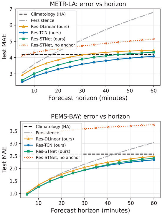
The anchor closes most of the gap to a strong climatology baseline. The improvements in Table 2, Table 3 and Table 4 are consistent in direction and size across both measurement types we study: Res-TCN improves on the holiday-aware climatology by 16.0% on METR-LA and 27.6% on PEMS-BAY, and by 13.8–22.0% on the four flow benchmarks, so the anchor’s benefit does not depend on a particular sensor network or on whether the signal is speed or flow. That the anchor, rather than the residual head alone, drives this result is clearest when it is removed: 60 min MAE degrades from 4.33 to 5.14 mph on METR-LA and from 2.42 to 3.76 mph on PEMS-BAY, with the degradation concentrated at exactly the long horizons where climatology carries most of the signal. The graph-based Res-STNet trails the non-spatial Res-TCN on both speed datasets, a pattern we return to below.

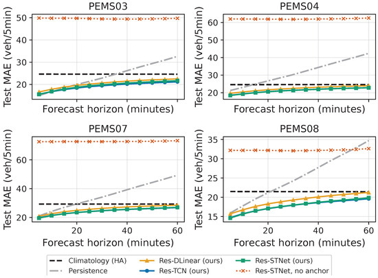
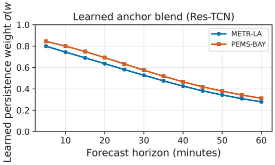
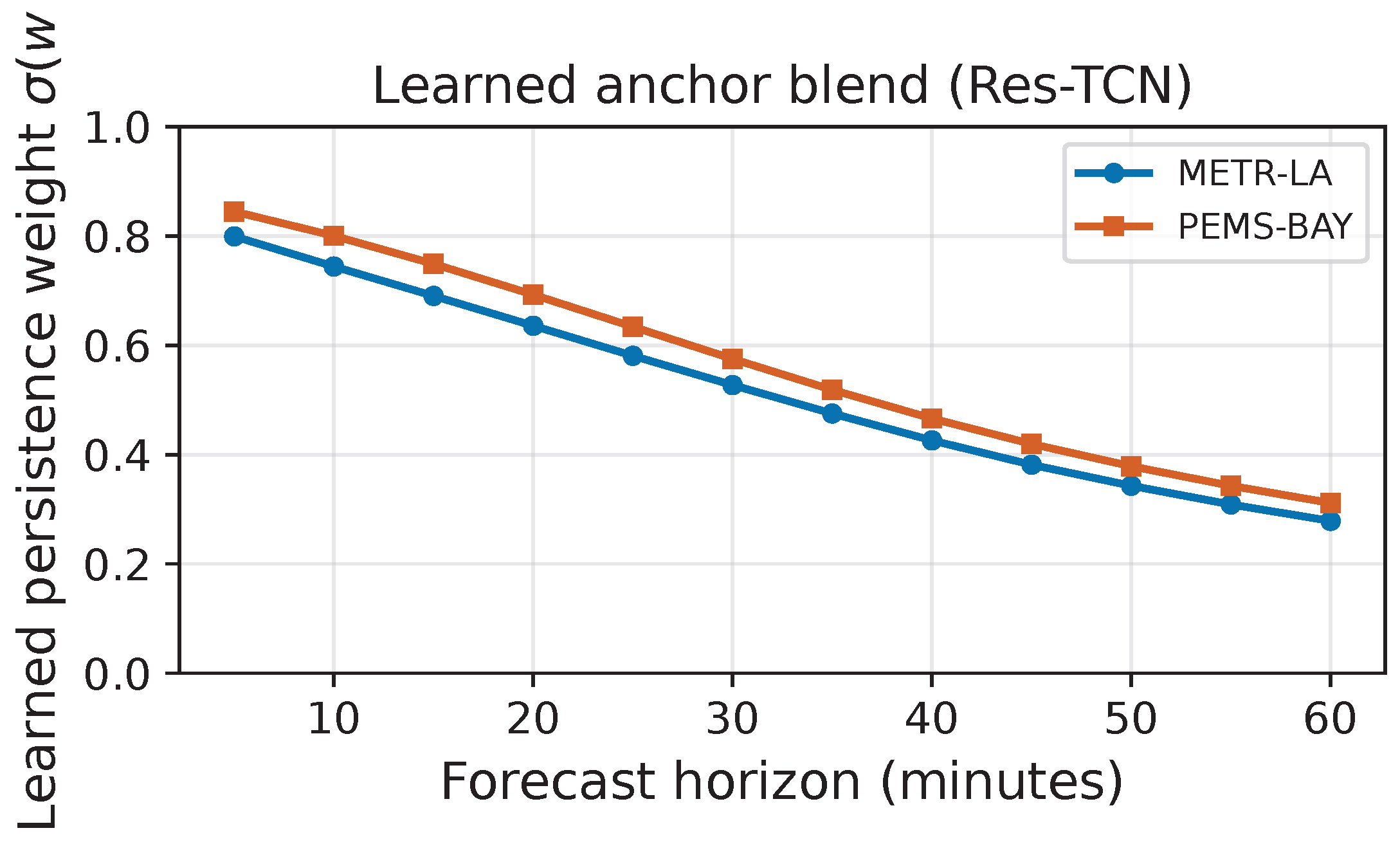
The learned blend recovers the regime-appropriate baseline at each horizon. Figure 1 and the ablation table show that removing the anchor degrades error sharply with horizon, whereas the learned blend keeps the temporal models at or below both baselines everywhere. On PEMS-BAY, the climatology-only anchor is beaten by persistence at short horizons; the learned blend recovers the persistence regime there and the climatology regime at long horizons, the mechanism behind the all-horizon win. With limited capacity (Res-DLinear), the residual head cannot fully cover the extreme horizons, so DLinear crosses the better baseline slightly there while still winning on average; the all-horizon win is realised once the head is expressive enough (Res-TCN, Res-STNet) as seen in Figure 1 (speed) and Figure 2. The learned weights are interpretable. The per-horizon persistence weight $\sigma \left(w_h\right)$ decays monotonically across all 12 horizons (Figure 3), on METR-LA from 0.80 at the 5 min horizon to 0.28 at 60 min, and on PEMS-BAY, from 0.84 at the 5 min horizon to 0.31 at 60 min (Res-TCN, seed-stable): with no supervision beyond the forecasting loss, the model discovers “trust the last observation short-term, the climatology long-term”, a regime structure a fixed anchor cannot express.

Figure 1. Test MAE versus forecast horizon on METR-LA (top) and PEMS-BAY (bottom).

Figure 2. Test MAE versus horizon on the four flow benchmarks PEMS03/04/07/08 (veh/5 min).

Figure 3. Learned per-horizon persistence weight $\sigma \left(w_h\right)$ of the Res-TCN anchor.

The shape transfers across datasets; the level does not. Table 20 reports $\sigma \left(w_h\right)$ (Res-TCN) at five horizons on all six benchmarks. The monotone-decay shape recurs everywhere, and every dataset trusts persistence most at 5 min and climatology most at 60 min, so the qualitative rule the anchor discovers is not specific to one sensor network. The evel is not transferable: the two speed datasets start near $\sigma \approx 0.80$–$0.84$ at 5 min, while the four flow datasets start markedly lower ($\sigma \approx 0.55$–$0.65$), i.e., the flow networks trust climatology more even at the shortest horizon. This mirrors the regime-dependence that motivates the anchor in the first place (Section 4.1): the mechanism is transferable as a rule, but its learned operating point is, correctly, dataset-specific. We also check stability across training seeds (Table 21): on METR-LA and PEMS-BAY, retraining Res-TCN on seeds $\{1,2,42\}$ reproduces the same weight profile to within 0.02 at every reported horizon, so the learned rule is a property of the data, not of a particular initialisation.

Table 20. Learned persistence weight $\sigma \left(w_h\right)$ (Res-TCN, seed 42) at five horizons across all six benchmarks. Values decay monotonically everywhere; the flow datasets (PEMS03/04/07/08) start lower than the speed datasets, i.e., they trust climatology more even at short horizons.

Dataset	5 min	15 min	30 min	45 min	60 min
METR-LA	0.799	0.690	0.527	0.381	0.278
PEMS-BAY	0.844	0.749	0.575	0.419	0.311
PEMS03	0.551	0.446	0.359	0.302	0.260
PEMS04	0.557	0.467	0.369	0.300	0.253
PEMS07	0.651	0.553	0.451	0.377	0.315
PEMS08	0.629	0.543	0.455	0.396	0.344

Table 21. Seed stability of the learned persistence weight $\sigma \left(w_h\right)$ (Res-TCN) at three horizons, seeds $\{42,1,2\}$.

Dataset	Seed	5 min	30 min	60 min
METR-LA	42	0.799	0.527	0.278
	1	0.803	0.532	0.281
	2	0.802	0.535	0.286
PEMS-BAY	42	0.844	0.575	0.311
	1	0.842	0.559	0.275
	2	0.845	0.565	0.290

The graph branch does not help within our lightweight family. In line with the literature questioning whether graph machinery is necessary [15,19], our spatial model (Res-STNet) is worse than the non-spatial Res-TCN on the speed datasets, significantly so under the paired bootstrap and on every seed (Table 18), and the learned adjacency is indistinguishable from a fixed physical graph. The zero-initialised-graph control (Section 4.7) shows this is not merely a bad initialisation. We scope the result to our lightweight family and budget: spatial structure is not useless in general, since the strong DCRNN/Graph WaveNet architectures (Section 4.4) beat all our lightweight predictors and our own anchored Graph WaveNet edges out Res-TCN by a thin margin.

6. Conclusions

Treating the regime-dependence of trivial baselines as a design principle rather than an obstacle yields a simple mechanism, a learned horizon-adaptive blend of persistence and climatology used as a residual anchor, that allows a learned temporal model to reliably beat two baselines on real data across six benchmarks spanning traffic speed and traffic flow, even against a strengthened holiday-aware climatology: at every horizon on five of the six datasets and on the 12-step average on all six (on PEMS03, persistence edges it only at the two shortest horizons). On these well-trained models, the average effect is small, but the regime structure persists at horizon resolution: on bursty METR-LA, the anchor hurts Graph WaveNet slightly at short horizons and helps it clearly at long ones, where climatology is informative, so its benefit concentrates exactly where the regime rewards it and fades where the model already has that information. Within our own lightweight family, the anchor, not architectural complexity, is what drives the improvements. Additionally, a non-spatial temporal model is sufficient to capture the gain, and the learned spatial graph adds minimal value relative to its parameter cost. This scopes the practical takeaway precisely: the stronger DCRNN and Graph WaveNet architectures still lead on absolute accuracy, but the anchor recovers a comparable share of their advantage at a fraction of the parameters and inference latency (Section 4.5), which is what recommends it for settings where a lightweight model is preferred.

References

- Li, Y.; Yu, R.; Shahabi, C.; Liu, Y. Diffusion convolutional recurrent neural network: Data-driven traffic forecasting. In Proceedings of the International Conference on Learning Representations (ICLR), Vancouver, BC, Canada, 30 April–3 May 2018. [Google Scholar]
- Yu, B.; Yin, H.; Zhu, Z. Spatio-temporal graph convolutional networks: A deep learning framework for traffic forecasting. In Proceedings of the International Joint Conference on Artificial Intelligence (IJCAI), Stockholm, Sweden, 13–19 July 2018; pp. 3634–3640. [Google Scholar] [CrossRef] [Scilit] [PubMed]
- Wu, Z.; Pan, S.; Long, G.; Jiang, J.; Zhang, C. Graph wavenet for deep spatial-temporal graph modeling. In Proceedings of the International Joint Conference on Artificial Intelligence (IJCAI), Macao, China, 10–16 August 2019; pp. 1907–1913. [Google Scholar] [CrossRef] [Scilit] [PubMed]
- Shao, Z.; Zhang, Z.; Wang, F.; Wei, W.; Xu, Y. Spatial-temporal identity: A simple yet effective baseline for multivariate time series forecasting. In Proceedings of the 31st ACM International Conference on Information and Knowledge Management (CIKM), Atlanta, GA, USA, 17–21 October 2022; pp. 4454–4458. [Google Scholar] [CrossRef] [Scilit]
- Zeng, A.; Chen, M.; Zhang, L.; Xu, Q. Are transformers effective for time series forecasting? In Proceedings of the AAAI Conference on Artificial Intelligence, Washington, DC, USA, 7–14 February 2023; Volume 37, pp. 11121–11128. [Google Scholar] [CrossRef] [Scilit]
- Guo, S.; Lin, Y.; Feng, N.; Song, C.; Wan, H. Attention based spatial-temporal graph convolutional networks for traffic flow forecasting. In Proceedings of the AAAI Conference on Artificial Intelligence, Honolulu, HI, USA, 27 January 2019; Volume 33, pp. 922–929. [Google Scholar] [CrossRef] [Scilit]
- Song, C.; Lin, Y.; Guo, S.; Wan, H. Spatial-temporal synchronous graph convolutional networks: A new framework for spatial-temporal network data forecasting. In Proceedings of the AAAI Conference on Artificial Intelligence, New York, NY, USA, 7–12 February 2020; Volume 34, pp. 914–921. [Google Scholar] [CrossRef] [Scilit]
- Chen, C.; Petty, K.; Skabardonis, A.; Varaiya, P.; Jia, Z. Freeway performance measurement system: Mining loop detector data. Transp. Res. Rec. 2001, 1748, 96–102. [Google Scholar] [CrossRef] [Scilit]
- Bai, L.; Yao, L.; Li, C.; Wang, X.; Wang, C. Adaptive graph convolutional recurrent network for traffic forecasting. In Proceedings of the Advances in Neural Information Processing Systems (NeurIPS), Virtual, 6–12 December 2020; Volume 33, pp. 17804–17815. [Google Scholar]
- Wu, Z.; Pan, S.; Long, G.; Jiang, J.; Chang, X.; Zhang, C. Connecting the dots: Multivariate time series forecasting with graph neural networks. In Proceedings of the 26th ACM SIGKDD International Conference on Knowledge Discovery & Data Mining, Jeju, Republic of Korea, 23–27 August 2020; pp. 753–763. [Google Scholar] [CrossRef] [Scilit]
- Zheng, C.; Fan, X.; Wang, C.; Qi, J. Gman: A graph multi-attention network for traffic prediction. In Proceedings of the AAAI Conference on Artificial Intelligence, New York, NY, USA, 7–12 February 2020; Volume 34, pp. 1234–1241. [Google Scholar] [CrossRef] [Scilit]
- Jiang, R.; Wang, Z.; Yong, J.; Jeph, P.; Chen, Q.; Kobayashi, Y.; Song, X.; Fukushima, S.; Suzumura, T. Spatio-temporal meta-graph learning for traffic forecasting. In Proceedings of the AAAI Conference on Artificial Intelligence, Washington, DC, USA, 7–14 February 2023; Volume 37, pp. 8078–8086. [Google Scholar] [CrossRef] [Scilit]
- Liu, H.; Dong, Z.; Jiang, R.; Deng, J.; Deng, J.; Chen, Q.; Song, X. Spatio-temporal adaptive embedding makes vanilla transformer sota for traffic forecasting. In Proceedings of the 32nd ACM International Conference on Information and Knowledge Management (CIKM), Birmingham, UK, 21–25 October 2023; pp. 4125–4129. [Google Scholar] [CrossRef] [Scilit]
- Wang, J.; Jiang, J.; Jiang, W.; Li, C.; Zhao, W.X. Libcity: An open library for traffic prediction. In Proceedings of the 29th ACM SIGSPATIAL International Conference on Advances in Geographic Information Systems, Beijing, China, 2–5 November 2021; pp. 145–148. [Google Scholar] [CrossRef] [Scilit]
- Shao, Z.; Wang, F.; Xu, Y.; Wei, W.; Yu, C.; Zhang, Z.; Yao, D.; Sun, T.; Jin, G.; Cao, X.; et al. Exploring progress in multivariate time series forecasting: Comprehensive benchmarking and heterogeneity analysis. IEEE Trans. Knowl. Data Eng. 2025, 37, 291–305. [Google Scholar] [CrossRef] [Scilit]
- Zhang, J.; Zheng, Y.; Qi, D. Deep spatio-temporal residual networks for citywide crowd flows prediction. In Proceedings of the AAAI Conference on Artificial Intelligence, San Francisco, CA, USA, 4–9 February 2017; pp. 1655–1661. [Google Scholar] [CrossRef] [Scilit]
- Oreshkin, B.N.; Carpov, D.; Chapados, N.; Bengio, Y. N-beats: Neural basis expansion analysis for interpretable time series forecasting. In Proceedings of the International Conference on Learning Representations (ICLR), Addis Ababa, Ethiopia, 26–30 April 2020. [Google Scholar]
- Cui, Y.; Xie, J.; Zheng, K. Historical inertia: A neglected but powerful baseline for long sequence time-series forecasting. In Proceedings of the 30th ACM International Conference on Information and Knowledge Management (CIKM), Gold Coast, Australia, 1–5 November 2021; pp. 2965–2969. [Google Scholar] [CrossRef] [Scilit]
- Liu, X.; Xia, Y.; Liang, Y.; Hu, J.; Wang, Y.; Bai, L.; Huang, C.; Liu, Z.; Hooi, B.; Zimmermann, R. Do we really need graph neural networks for traffic forecasting? arXiv 2023, arXiv:2301.12603. [Google Scholar] [CrossRef] [Scilit]
- Rasp, S.; Dueben, P.D.; Scher, S.; Weyn, J.A.; Mouatadid, S.; Thuerey, N. Weatherbench: A benchmark data set for data-driven weather forecasting. J. Adv. Model. Earth Syst. 2020, 12, e2020MS002203. [Google Scholar] [CrossRef] [Scilit]
- Hyndman, R.J.; Koehler, A.B. Another look at measures of forecast accuracy. Int. J. Forecast. 2006, 22, 679–688. [Google Scholar] [CrossRef] [Scilit]
- Kwak, S. PEMS-BAY and METR-LA in csv (Version v5) [Dataset]. Zenodo, 2020. Available online: https://zenodo.org/records/5146275 (accessed on 10 June 2026).
- Huang, X. California Traffic Network Datasets: PEMS03, PEMS04, PEMS07 and PEMS08 for Traffic Flow Forecasting [Dataset]. IEEE DataPort, 2025. Available online: https://ieee-dataport.org/documents/california-traffic-network-datasets-pems03-pems04-pems07-and-pems08-traffic-flow (accessed on 10 June 2026).
- Künsch, H.R. The jackknife and the bootstrap for general stationary observations. Ann. Stat. 1989, 17, 1217–1241. [Google Scholar] [CrossRef] [Scilit]
- Politis, D.N.; Romano, J.P. The stationary bootstrap. J. Am. Stat. Assoc. 1994, 89, 1303–1313. [Google Scholar] [CrossRef]
- Diebold, F.X.; Mariano, R.S. Comparing predictive accuracy. J. Bus. Econ. Stat. 1995, 13, 253–263. [Google Scholar] [CrossRef] [Scilit]
Disclaimer/Publisher’s Note: The statements, opinions and data contained in all publications are solely those of the individual author(s) and contributor(s) and not of MDPI and/or the editor(s). MDPI and/or the editor(s) disclaim responsibility for any injury to people or property resulting from any ideas, methods, instructions or products referred to in the content. |
© 2026 by the authors. Licensee MDPI, Basel, Switzerland. This article is an open access article distributed under the terms and conditions of the Creative Commons Attribution (CC BY) license.