Hierarchical Graph Representation Learning for ECG Classification with Cross-Dataset Generalization

Abstract

In this research, we propose a graph-based approach to classify ECG signals. We model the ECG signal as a time-varying graph and examine its dynamics at two levels: intra-beat and inter-beat. The proposed framework employs a two-level graph representation of the ECG. At the intra-beat level, each beat is modeled as a graph in which the P, Q, R, S, and T waves serve as nodes, and temporal distance information is incorporated into the node feature vector. At the inter-beat level, the ECG signal is represented as a graph of beats. We investigated two node representations: learnable MLP embeddings derived from handcrafted features and reduced features obtained via PCA. Unlike conventional temporal GCNs, graph attention networks (GATs), and transformers, which predominantly rely on single-level representations of ECG signals, the proposed approach builds hierarchical graph structures directly from ECG signals. The dual model was trained on 1024 ECG segments from the PTB Diagnostic ECG Database (PTBDB) and tested on 398 ECG segments from the MIT-BIH Arrhythmia Database to evaluate its performance. The results indicate that the best-performing configuration, which employs PCA-reduced node features, outperforms the other configurations tested. The model achieves a mean accuracy of $97.67\%$ and a mean F1-score of $97.18\%$ over five runs.

1. Introduction

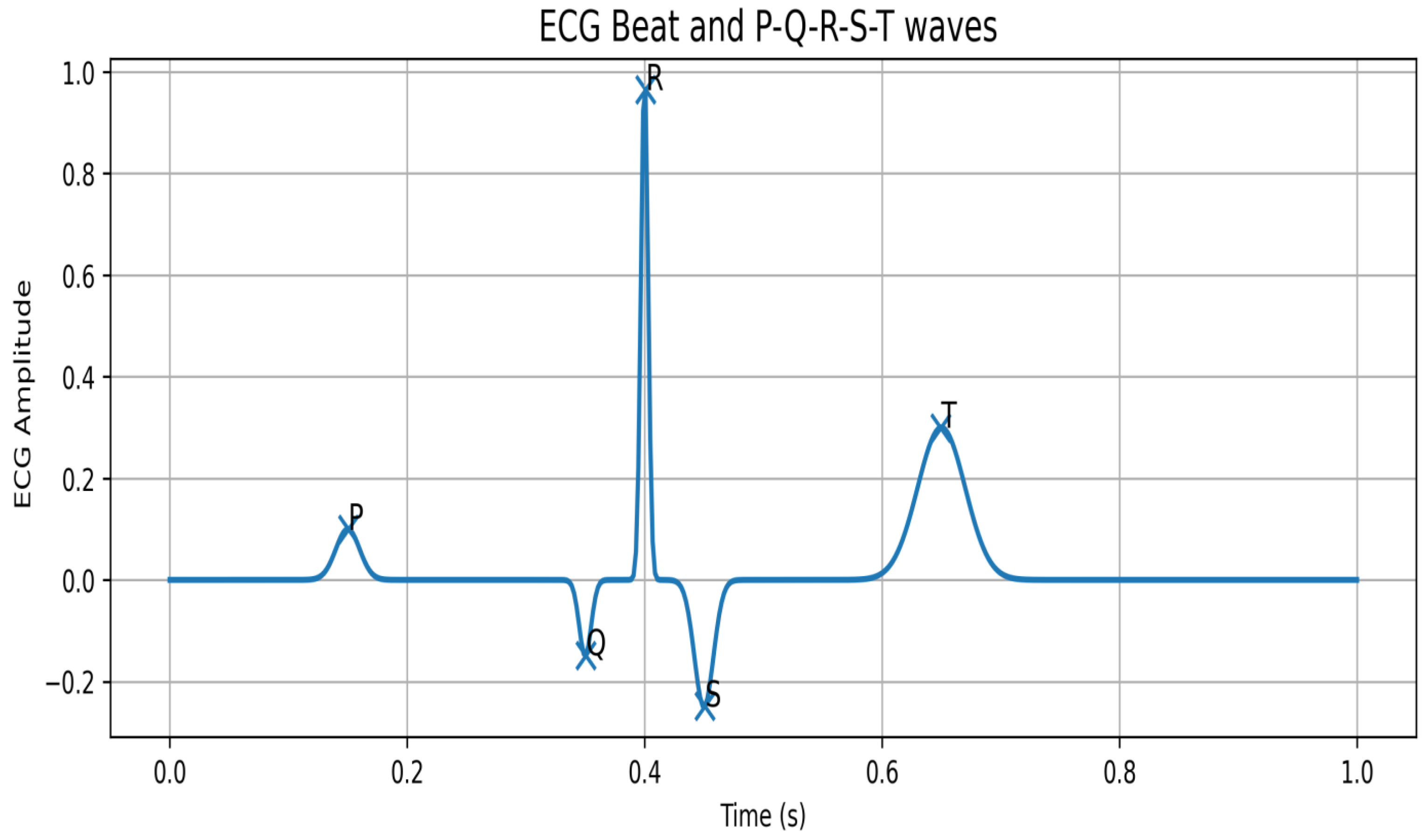
An electrocardiogram (ECG) is a graphical representation of cardiac cycles that illustrates the electrical activity of the heart. An ECG beat comprises the P wave, QRS complex, and T wave. The P wave depicts atrial depolarization, the QRS complex represents ventricular depolarization, and the T wave represents ventricular repolarization. An ECG beat with P-Q-R-S-T waves is shown in Figure 1.

Deep learning methods have been widely used to interpret ECG signals and, in several studies, have achieved higher accuracy than manual reading. These methods include Multilayer Perceptrons (MLPs), Recurrent Neural Networks (RNNs), Convolutional Neural Networks (CNNs), Long Short-Term Memory networks (LSTMs), and Transformers. MLPs are simple, efficient, and effective for limited discriminative features; however, they do not account for local temporal structure. CNNs extract discriminative features automatically without hand engineering and therefore often outperform MLPs. Hybrid CNN–RNN architectures are also used to classify ECG signals: CNNs detect local features, while RNNs capture contextual information in both directions, aiding the classification of long-duration recordings.

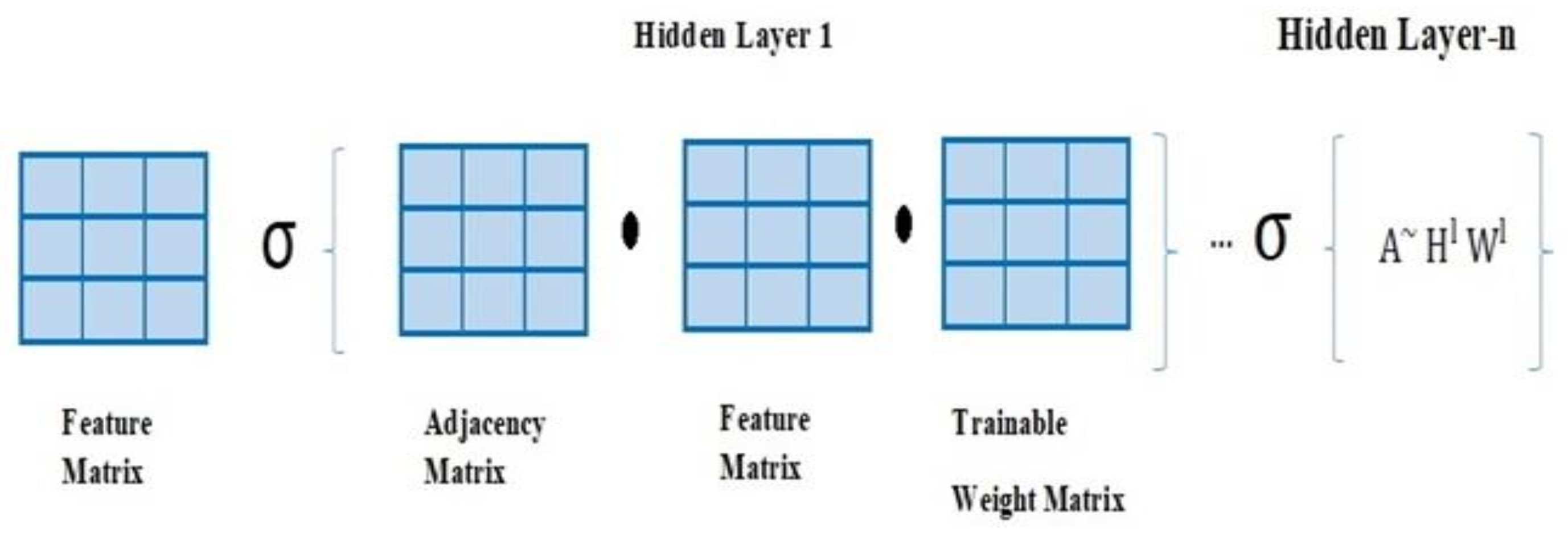
In a Graph Convolutional Network (GCN), each node corresponds to an entity, and edges represent interactions between entities. The primary objective of the GCN is to learn node embeddings—vector representations of nodes that incorporate not only the node’s features but also its interactions with neighboring nodes in the graph. The input size of GCNs can vary, making them particularly suitable for ECG signals.

Many previous studies have reported using GCNs for analyzing ECG signals and detecting various arrhythmias. For example, Lee et al. [1] proposed a GCN to detect and classify beats into normal, supraventricular, and ventricular ectopic categories. In their network, the P wave, QRS complex, and T wave serve as graph nodes. To improve feature extraction, a QRS-centered weighted average pooling method is used to enhance beat-specific feature extraction. A systematic approach is employed to find the optimal model design by investigating node features, GCN architecture, and edge descriptions. The dataset consists of a single 10 s lead ECG recording per patient from a total of 328 patients. Using 5-fold cross-validation, the proposed method achieved an F1 score of 88.61%, demonstrating that Graph Convolutional Networks can be beneficial in the context of electrocardiography. Xu and Xia [2] utilized a dynamic Graph Convolutional Neural Network to extract temporal information from ECG signals. Ma and Xia [3] employed a GCN to detect atrial fibrillation, where node features represent morphological features of heartbeats and edges represent the time intervals between heartbeats. The proposed model was evaluated on the MIT-BIH AFDB dataset and the Physionet Challenge 2017 AFDB dataset. The results indicate that the model is promising for detecting AF compared to other existing models.

GCN models that use pooling methods such as average pooling, max pooling, and add pooling often lose vital beat features. Although CNNs and RNNs are effective at analyzing local features and temporal dependencies in ECG data, they lack explicit modeling of the structured relationships among different physiological factors. The use of Temporal Graph Convolutional Networks enables the incorporation of structured relationships into ECG data analysis. However, these are typically applied at a single level and cannot discriminate between intra-beat and inter-beat temporal characteristics. Transformer models capture long-term dependencies using an attention mechanism within ECG data but still operate based on sequential modeling. There is therefore a need for an approach that integrates both temporal and structured features within ECG modeling.

We propose a GCN that represents the morphological, temporal, and spectral features of nodes to enhance its ability to learn beat-level information more effectively than from raw signals. First, we propose a graph representation with five nodes per beat, each representing the P, Q, R, S, and T points. Our model uses a ring topology due to its simplicity and physiological relevance. The nodes of the graph represent each of the five major waves in an electrocardiogram, namely P, Q, R, S, and T, where the ring preserves their chronological order and allows efficient information exchange between adjacent wave components. In contrast to the chain topology, the ring topology creates a direct link between the T and P waves, thereby emphasizing the cyclical pattern of cardiac activity and information flow throughout the entire graph. A fully connected graph would introduce numerous physiologically irrelevant connections, needlessly increasing computational complexity. In addition, learning the adjacency of the graph from data would require a significant number of parameters along with larger training datasets, making the resultant graph structure less interpretable. By using existing physiological knowledge for constructing the graph, the suggested ring topology acts as an appropriate inductive bias, with each node connected to two other nodes: P is connected to Q, Q to R, R to S, S to T, and T back to P. The edges represent intra-beat structural connections and reflect the structural relationships, temporal adjacency, and physiological order of the nodes. In contrast to previous models limited by fixed-length inputs, our GCN model handles variable-length ECG signals. We systematically evaluated multiple GCN architectures to identify the optimal design. In addition, we used different sets of ECG signal morphological, temporal, and spectral features to select the most appropriate set for accurate diagnosis.

Our method uses a novel approach that employs GCN to represent the ECG signal and thus illustrate the complex relationships in the data. In contrast to existing ECG-GNN methods that use sample-level graphs or generic connectivity, we represent each heartbeat as a physiologically constrained graph whose nodes correspond to clinically meaningful ECG waves (P-Q-R-S-T). Each node combines both local spectral characteristics and global morphological descriptors, enabling attention-based pooling to highlight diagnostically dominant cardiac phases. Second, we propose a representation in which each beat is a node with embedded features. The features are extracted from a set of representative time-domain and frequency-domain features to classify normal and abnormal segments.

We summarize our method as follows:

• Apply global normalization to the ECG signal as an essential preprocessing step that reduces differences in heart rate, position, and amplitude. We applied min–max scaling, which is an amplitude normalization that resizes amplitudes to a fixed range.
• Apply a simple peak detection approach to identify the R-peaks, which serve as landmarks for heartbeats, and then for each detected R-peak, specify the P, Q, S, and T points to perform ECG segmentation.
• Extract different morphological, temporal, and spectral features and form different sets of features to examine the most appropriate set for beat detection.
• Evaluate different ECG graph representations to find the optimal representation for detecting arrhythmia.

Our experiments demonstrate the significant value of GCNs, which use graph-based deep learning to classify ECG signals and detect different arrhythmia types. The results validate the proposed approach and provide a novel perspective on the effectiveness of graph representations in arrhythmia detection, particularly for the illustration and analysis of complex sequential data such as ECG signals.

The main contributions of this work are the following:

• A two-level graph representation that models the ECG at both the intra-beat and inter-beat levels, capturing multi-scale temporal dependencies.
• A feature engineering approach that utilizes morphological, temporal, and spectral features in graph representations.
• A cross-dataset evaluation, in which the model is trained on one database and tested on segments of a different database to assess generalization.

Deep learning techniques have been widely used for ECG classification. However, further research is still required. Graph Neural Networks (GNNs) have recently also been used for ECG analysis by representing ECG signals as graphs. However, ECG-GraphNet and Temporal Graph Convolutional Networks have achieved higher accuracy in ECG classification by exploiting relationships within ECG feature data. Most of these methods use only one level of graphs, where either ECG signal segments or features form the nodes of a graph. This implies that none of these methods explicitly discriminates between relations among wave components of one cardiac cycle (intra-beat relations) and successive cardiac cycles (inter-beat relations).

Intra-beat and inter-beat relationships contain crucial information for ECG diagnosis. Intra-beat relationships represent morphological features, while inter-beat relationships refer to rhythm dynamics. Modeling these two different types of relationships within a single consistent framework poses a challenge in the field of ECG classification. Moreover, despite good performance on specific datasets, most previous studies lack cross-dataset validation and thus may not perform well in other clinical settings.

The present work proposes a two-level hierarchical graph representation for ECG classification, inspired by the physiological knowledge of the cardiovascular system. Specifically, intra-beat relationships within ECG waves are represented as graph nodes at the first level, and heartbeats are represented as nodes in a temporal graph to model inter-beat relationships at the second level.

2. Literature Review

2.1. Background

In this section, we provide an overview of GCNs and highlight their architectural insights. While Convolutional Neural Networks (CNNs) process grid-like data representations, GCNs handle graph-structured data, which makes them powerful deep learning models appropriate for non-Euclidean data and useful in fields such as social networks, molecular structures, and recommendation systems. A graph is defined as G = (V, E), where V is the set of nodes and E is the set of edges. Each node v in V has features Xv that represent the initial features or learned embeddings. In the graph, the nodes represent the entities, while the edges describe the relationships between them. The adjacency matrix describes the graph’s structure and indicates which nodes are connected. The GCN model learns about the graph structure via graph-structured embeddings. GCNs consist of multiple layers, each capable of improving node embeddings by combining information from distant neighbors. The layers are:

1.

Input layer: The input layer accepts node features or pre-trained node embeddings.

2.

Hidden Layers: The hidden layers contain the following:

• Convolutional Layers: These layers update the node’s feature representation based on the node and its neighbors’ information.
• Pooling Layers: These layers aggregate nodes to reduce the graph size, enabling the model to learn hierarchical relationships more efficiently.
• Activation functions, such as ReLU, are used after each convolutional layer to enhance the model’s ability to learn more complex patterns.

3.

Output Layer: The output layer produces the final prediction or node embeddings.

4.

Fully Connected Layers: Flatten the learned embedding to produce the final prediction.

The Architecture of GCN is represented in Figure 2.

The main operation in a GCN layer is given by:

$$H^{(l+1)}=\sigma \left(\tilde{A}{H}^{\left(l\right)}{W}^{\left(l\right)}\right)$$

(1)

where

• $H^{\left(l\right)}$ is the matrix of node features at layer l,
• $\tilde{A}$ is the normalized adjacency matrix,
• $W^{\left(l\right)}$ is the trainable weight matrix at layer l,
• $\sigma$ is an activation function, such as ReLU.

2.2. Related Works

In this section, we summarize related literature on ECG record classification and highlight its strengths and limitations. MLPs have been widely used to analyze ECG signals [4,5,6,7,8,9,10,11]. MLPs remain useful for ECG analysis and classification, particularly with hand-engineered features and small-scale models. MLPs are simple and efficient when precise hand-engineered features are provided; however, they lack the temporal dependency learning capabilities of CNNs and RNNs. CNNs do not require prior domain knowledge to extract features. They allow direct input of ECG signals to learn key features. They are widely used to detect and classify ECG signals [12,13,14,15,16,17]. Still, they have a fixed input length, which is a restriction when processing variable-length signals; in addition, they have difficulty effectively capturing temporal dependencies in sequential data. RNNs/LSTMs are also used for analyzing ECG signals and classification [18,19,20,21]. They can handle models with temporal dependencies and variable-length signals and capture changes over time in ECG signal patterns, but they have a high computational cost for large datasets and have a fixed input length. Transformer-based models prove useful for analyzing electrocardiogram signals, as they can detect long-term temporal dependencies and dependencies between distant regions of a waveform. Nevertheless, transformer-based models often require large training sets, powerful computational resources, and regularization techniques due to their vulnerability to overfitting [22,23,24,25].

A list of representative deep learning-based ECG classifiers is summarized in

Table 1. Comparison of Existing ECG Classification Approaches with the Proposed Method.

Method	Function	Approach	Strengths	Limitations	Proposed Method Characteristics
CNN-based	CNN arrhythmia classification	Local waveform features	Strong morphology learning	No long temporal or structural modeling	Adds temporal and structural graph modeling.
CNN–RNN Hybrid	CNN–RNN attention ECG model	CNN + sequence modeling	Captures temporal dependencies	No explicit structure modeling	Models physiological relationships using graphs.
Transformer-based	Transformer ECG classification	Self-attention sequence learning	Long-range dependency modeling	Ignores physiological structure	Introduces physiologically structured ECG graphs.
GCN-based	ECG-GraphNet	Graph representation of ECG	Captures feature relationships	Single-level representation	Uses two-level hierarchical graphs.
Temporal GCN	MST-DGCN	Graph + temporal modeling	Captures temporal dependencies	No intra-/inter-beat separation	Separates intra-beat and inter-beat levels.
Hybrid GCN+DL	BiLSTM–GCN	Temporal + graph hybrid	Good performance	Not a unified representation	Provides a unified graph architecture.
Proposed Method	This Work	Two-level hierarchical graph + features	Captures multi-scale dependencies	Requires graph design	Provides physiologically guided intra- and inter-beat graph modeling.

. Deep learning-based models using CNNs have been shown to be powerful for local morphological feature learning; however, such models provide limited explicit representation of physiological structure between different ECG components. CNN/RNN hybrids and Transformer networks show significant improvements in capturing temporal dependencies; however, these models still treat ECG signals as sequences and lack the ability to represent relationships among ECG components based on physiological knowledge. Graph neural network-based solutions can better model the structure of ECGs but typically represent ECGs as single-level graphs. Single-level graphs usually capture either morphological relationships or temporal dependencies; they do not represent intra-beat and inter-beat relationships together in one framework.

The limitations discussed above motivate the development of the two-level graph architecture. The following section presents the methodology, including dataset preparation, label harmonization, intra-beat GCN, inter-beat GCN, two-level graph representation, and hyperparameters.

3. Methodology

3.1. Dataset Preparation and Patient-Wise Segmentation

The proposed framework was developed on the PTBDB. Throughout this study, the reported sample sizes refer to ECG segments, not to the original recordings in the databases. Each recording was preprocessed and divided into non-overlapping 5 s segments, which increased the number of samples while preserving the temporal characteristics of the signal. To avoid subject-level leakage, we applied a patient-wise split before segmentation: all recordings from a given patient were placed in a single set, so no patient appeared in more than one set. The training and validation sets were both drawn from PTBDB in this patient-wise manner. The MIT-BIH Arrhythmia Database was held out entirely and used only for the final external test; it was not used for validation, early stopping, or any model selection. The MIT-BIH database contains 48 annotated records from 47 subjects, each approximately 30 min long and sampled at 360 Hz. Each record was split into non-overlapping 5 s segments. Because the PTBDB recordings were originally sampled at 1000 Hz, they were resampled to 360 Hz to match MIT-BIH, ensuring that each 5 s segment contained 1800 samples in both databases. After segmentation, 1024 PTBDB segments were used for model development, and 398 MIT-BIH segments were used for external testing.

The beat-level experiments (Experiments 1–3) draw on a partially distinct pool of source recordings than the record-level experiments. On the training side, approximately 30% of the 20,000 PTBDB training beats (≈6000 beats) were extracted from the same 1024 PTBDB segments used in the record-level experiments, while the remaining ≈70% (≈14,000 beats) were extracted from additional PTBDB recordings belonging to patients already assigned to the training set, preserving the patient-wise split described above. On the test side, the 4029 MIT-BIH beats used for external testing were extracted entirely from MIT-BIH recordings distinct from the 398 segments used in the record-level test set, with no overlap between the two beat- and segment-level test pools; these additional recordings were likewise drawn exclusively from the held-out MIT-BIH test patients. Consequently, no beat-level or record-level data crosses between the training and test partitions at either granularity.

Table 2. Recordings, segments, and beats used across all experiments.

Database (Role)	Recordings/Subjects	Segments (5 s)	Beats
PTBDB (Training)	250 records	1024	20,000
MIT-BIH (Test)	48 records, 47 subjects	398	4029

summarizes the number of recordings, segments, and beats used across all experiments in both databases.

3.2. Label Harmonization

Since the PTBDB Diagnostic ECG Database and the MIT-BIH Arrhythmia Database used distinct annotation standards, their original labels had to be converted to a common binary system before developing the models. The PTBDB offers clinical diagnoses for individual subjects or records. Records from healthy subjects were classified as normal. In contrast, those associated with myocardial infarction, cardiomyopathy/heart failure, bundle branch block, dysrhythmia, myocardial hypertrophy, valvular heart disease, myocarditis, or other cardiovascular problems were classified as abnormal. Subjects for whom a definitive clinical diagnosis was unavailable were not included in the labeled dataset. After the segmentation process, each 5 s PTBDB record was assigned a label matching the source record’s label.

The MIT-BIH Arrhythmia Dataset includes expert annotations at the individual heartbeat level. These were first classified into standard coarse-grained beat classes and then into the corresponding binary label space. A 5 s MIT-BIH excerpt was classified as normal if all the annotated beats in the excerpt were of the normal beat type. If one or more supraventricular ectopic, ventricular ectopic, or fusion beats were found in the excerpt, it was considered abnormal. Paced, unclassifiable, or noise-contaminated excerpts were removed to prevent any ambiguity in the labels. This mapping ensured that the target of normal versus abnormal classification was consistent across both datasets.

3.3. Intra-Beat GCN

The nodes are connected in a ring topology, where each node is linked to exactly two neighbors and the edges follow the physiological order of the waves. P is connected to Q, Q is connected to R, R is connected to S, S is connected to T, and T is connected back to P. The edge between T and P closes the ring and reflects the cyclic nature of the cardiac cycle, allowing information to flow between the end of one beat and the start of the next. We used bidirectional edges, which allow information to travel in both directions and lead to more stable learning.

Every single beat forms a graph, so the ECG record is represented by a set of graphs. The graph representation enhances the GCN’s ability to analyze the ECG signal. (1) We first apply min–max normalization to reduce variability and improve stability across the dataset. (2) We applied a threshold-based peak detection algorithm to identify R-peaks. An R-peak corresponds to a local maximum in the sample. A local maximum is accepted as an R-peak if its amplitude exceeds a predefined threshold and it is separated from neighboring peaks by a minimum distance. Each identified R-peak marks the midpoint of a cardiac cycle. For an R-peak at index r, the beat is extracted over the window [$r-0.35f_s$, $r+0.45f_s$] where fs is the sampling frequency. (3) We performed beat segmentation by finding P, Q, S, and T points relative to the R-peak. Every P-Q-R-S-T represents a single beat. P and T waves are recognized as local maxima, while Q and S waves are recognized as local minima within predefined windows. (4) We constructed a graph G = (V, E) for each heartbeat, where V represents the graph nodes, which are P, Q, R, S, and T points. The edge set (E) has a ring topology.

Each node is represented by a set of local time–frequency features and global morphological features. This set of representative features enables the GCN to learn both intra-beat structure and inter-wave associations. We propose edge definitions that represent morphological and spectral ECG features. The node feature matrix captures crucial characteristics for effective beat classification. For each node, we applied three feature groups and validated them; local features are extracted from a small window around the node position, containing amplitude and spectral features such as dominant frequency, spectral entropy, and band power. Various global beat-level features, such as QRS duration, PR interval, ST interval, R-peak amplitude, and beat slope, are computed and added to each node’s feature vector. The amplitude represents the normalized voltage at the ECG beat, scaled to [0, 1] to enhance the GCN’s ability to focus on local shape. The amplitude illustrates the strength of the heart’s electrical activity. The dominant frequency is the highest magnitude in the beat frequency spectrum and corresponds to the frequency shift. A sharp change in the heartbeat indicates an abnormal heartbeat. Spectral entropy is used to estimate the uniformity of the power distribution across the frequency domain of a signal. It detects deviations in beats and separates abnormal beats from normal ones. Spectral entropy is a measure of frequency complexity. Higher entropy values indicate abnormal behavior, while lower values indicate normal behavior. Band power measures the physiological energy content and captures factors that affect beat detection beyond heart-rate variability. We extracted these spectral features to reveal patterns that are not distinguishable in the raw ECG. QRS duration represents the depolarization time, and abnormalities can be detected based on this duration. The PR interval measures the time between atrial depolarization and the start of ventricular depolarization. The ST interval represents the time between the ventricular QRS complex and the T wave. R-peak amplitude is the maximum height of the R wave and is significant in ECG analysis. Beat slope demonstrates the speed of electrical activation.

These features capture beat context and enable the GCN to learn interaction conditions based on beat morphology; they also enhance training stability.

Group 1 (G1) includes amplitude, dominant frequency, and spectral entropy.

Group 2 (G2) includes ECG amplitude, spectral centroid, spectral bandwidth, and spectral flatness. The spectral centroid measures the center of mass of the frequency spectrum. Typically, P has a low spectral centroid (SC), which indicates a slow change; Q and S have medium values, while R has a high value, implying a very sharp transition, and T has a low value. SC is a crucial feature for detecting arrhythmia, as it can detect abnormal depolarization rate and thus differentiate between sharp and smooth waves. Spectral bandwidth indicates the spread of the spectrum around the centroid and measures the width of the frequency distribution. Typically, P has a narrow bandwidth, R is wideband, and T is also narrow. It describes the dimensionality of waveform shape. A wider bandwidth indicates an irregular shape. Spectral flatness is the ratio of the geometric mean to the arithmetic mean of the power spectrum. G2 uses complete spectral information to provide a robust representation of ECG morphology, enabling useful discrimination between normal and abnormal beats.

Group 3 (G3) includes two features for each of P, Q, R, S, and T: amplitude and time relative to R, in seconds. Each node is described by its normalized amplitude and temporal offset relative to the R-peak. This reflects the physiological nature of the ECG signal; G3 represents a low-dimensional feature node matrix that reduces overfitting and provides a useful inductive bias for the GCN. The set of feature groups is provided in

Table 3. Feature groups used to construct ECG graph node representations.

Group (1) G1		Group (2) G2		Group (3) G3
Class	Feature	Class	Feature	Class	Feature
Time-domain	Amplitude	Frequency-domain	Spectral Centroid	Time-domain	Amplitude
Frequency-domain	Dominant Frequency	Frequency-domain	Spectral Bandwidth	Time-domain	Time Relative to R (s)
Frequency-domain	Spectral Entropy	Frequency-domain	Spectral Flatness	–	–
–	–	Time-domain	Amplitude	–	–

. We conducted five experiments; in the first three, we used G1, G2, and G3. The architecture of the proposed GCN uses attentional graph pooling to learn the importance of each graph node. Attentional Graph Pooling is used instead of uniformly analyzing all nodes to construct a graph-level representation. In graph pooling, an attention score is assigned to each node based on its feature vector by the pooling layer, and the scores are normalized using a softmax function. The resulting graph embedding is calculated as the weighted sum of node embeddings.

3.4. Inter-Beat GCN

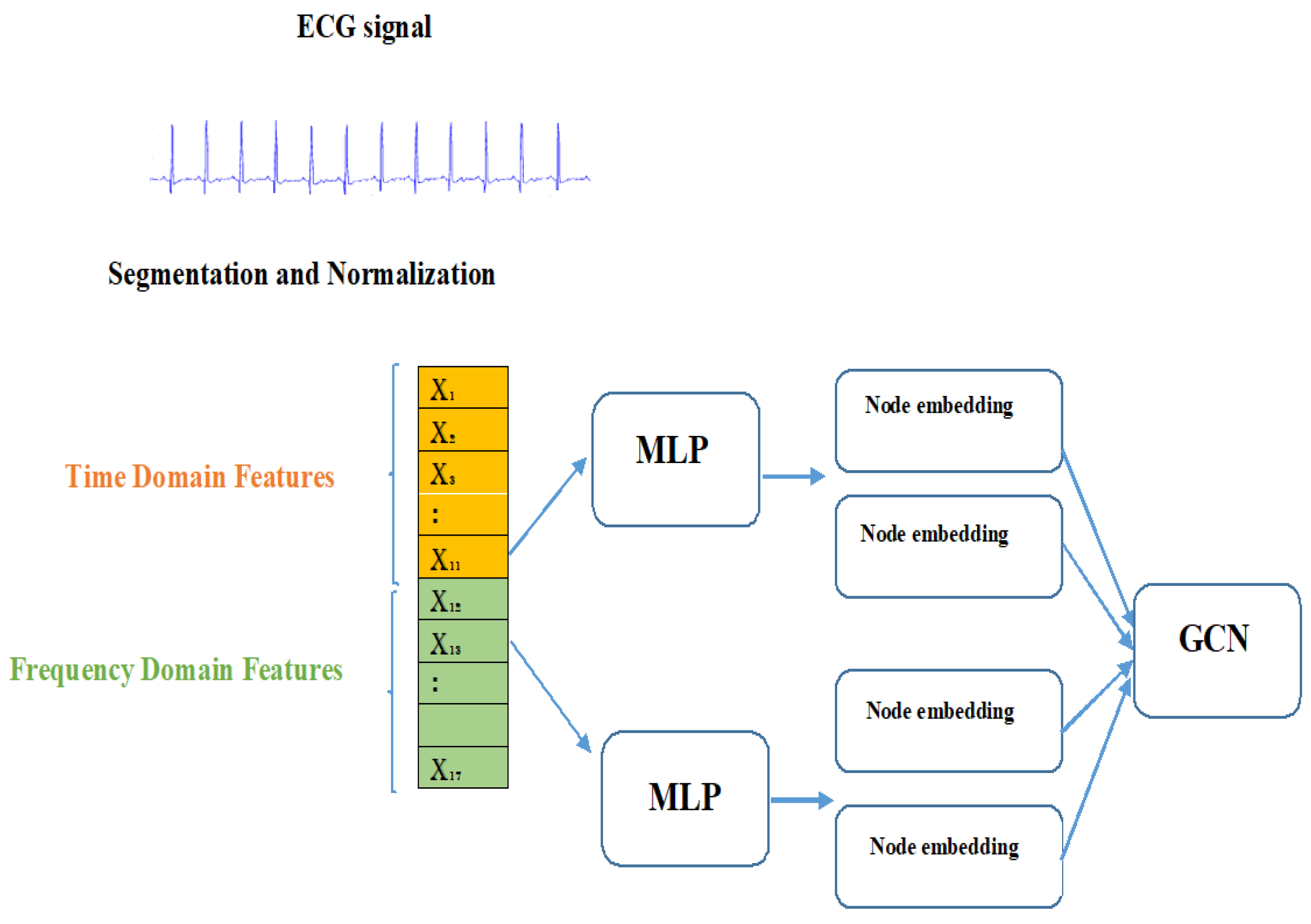
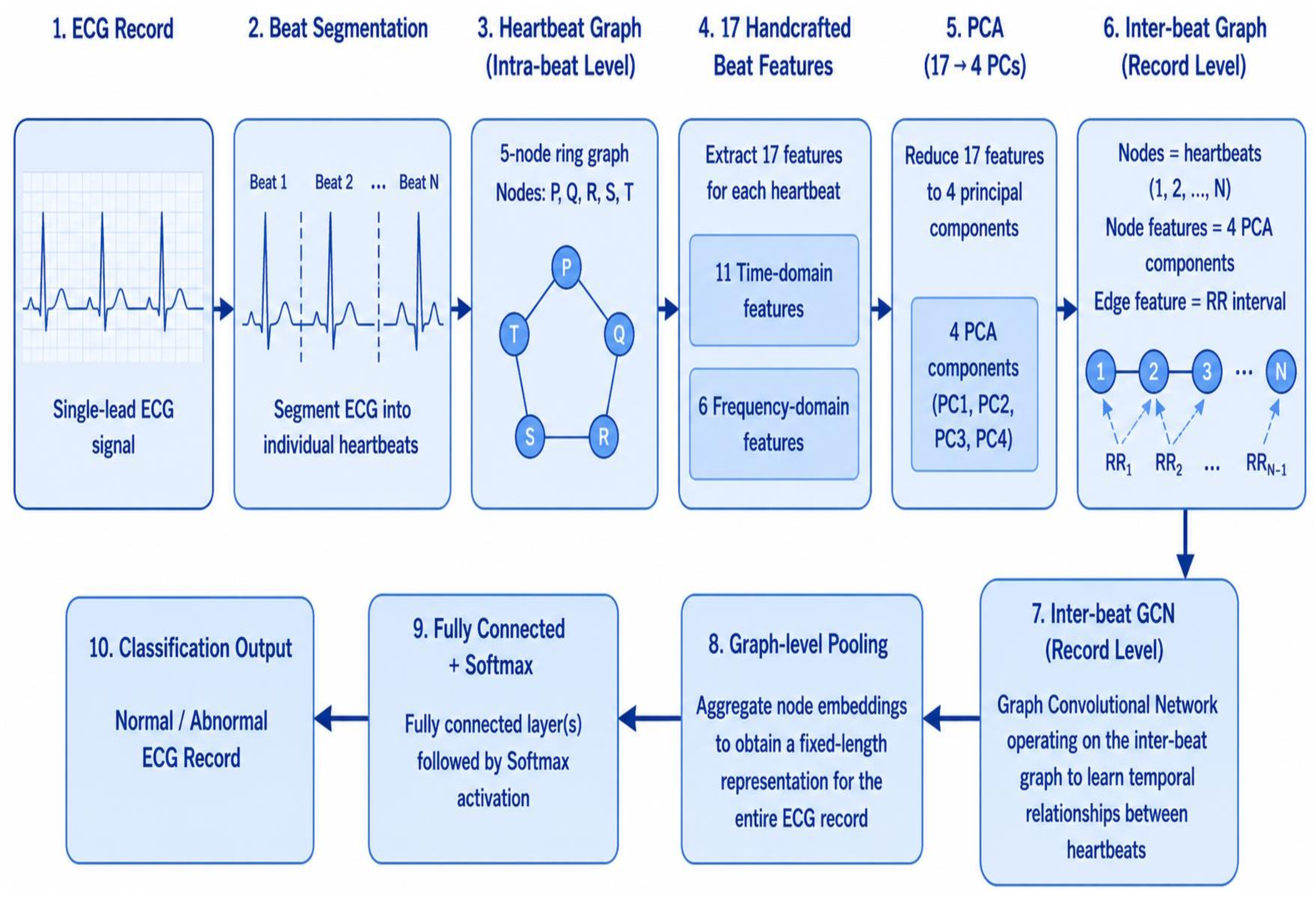
We propose a second GCN in which the whole record is represented as a single graph, with the beats considered as nodes. Initially, each beat was expressed in terms of a 17-dimensional handcrafted feature vector comprising eleven time-domain features and six frequency-domain features. To determine the impact of different feature representations on the model’s accuracy, two additional feature representation schemes were considered. In the first, the time-domain and frequency-domain features were independently embedded through two multilayer perceptrons to generate compact node embeddings. The second technique involved performing PCA on the initial feature vector to yield four principal components with minimal loss of variance.

In the fourth experiment, we extracted 17 features from the time and frequency domains of the signal detailed below. The time-domain features are computed directly from the ECG signal and from the ECG waveform. They illustrate the amplitudes and the time intervals between the cardiac points (P, Q, R, S, T). These features describe beat morphology and reflect the regularity and variability of beat rhythm. Frequency-domain features are computed from the fast Fourier transform (FFT) domain or the power spectrum. They describe energy and distribution across various frequencies. These features include the dominant frequency of the beat spectrum, spectral entropy, band power in the 0–40 Hz range, spectral centroid, spectral bandwidth, and spectral flatness. They represent signal complexity and describe abnormal electrical patterns. To perform the feature extraction phase, we detect R-peaks using a simple local-maximum rule with adaptive thresholding based on the signal amplitude and a minimum inter-peak distance of 200 ms. We tried several thresholds per record and retained records with at least two valid R-peaks. Then, we defined a window from 0.35 s before the R-peak to 0.45 s after to detect the P, Q, S, and T waves (P is detected in [$-0.25$ s, $-0.08$ s], Q is detected in [$-0.06$ s, $-0.01$ s], S is detected in [+0.01 s, +0.06 s], and T is detected in [+0.08 s, +0.40 s]).

Based on these points, we extracted 9 time-domain and 2 rhythm features, in addition to 6 frequency-domain features. Although time- and frequency-extracted features represent crucial detectors, they have non-discriminative parts. To solve this issue, we employed a learnable embedding mechanism that reduced the dimensionality of the extracted features to a low-dimensional embedding. The 17-dimensional node feature vector contains 11 time-domain features and 6-dimensional frequency-domain features. Each domain feature is independently fed into two multi-layer perceptrons (MLPs), which produce node embeddings; the first MLP embeds the time-domain features and the second MLP embeds the frequency-domain features into a low-dimensional space, and the two embeddings are concatenated to form the node feature. The learned embedding features form the feature matrix of each node (beat) in the graph. This helps the model learn better representations, reduces overfitting, and preserves the morphological and spectral content of the beat. After beat-level feature vectors have been obtained, each ECG record is transformed into a graph structure. Nodes represent individual beats, and edges illustrate temporal adjacency. Each beat is connected to its neighboring beats in the ECG record. The graph construction maintains beat-to-beat reliance while enabling the GCN to aggregate information across beats. 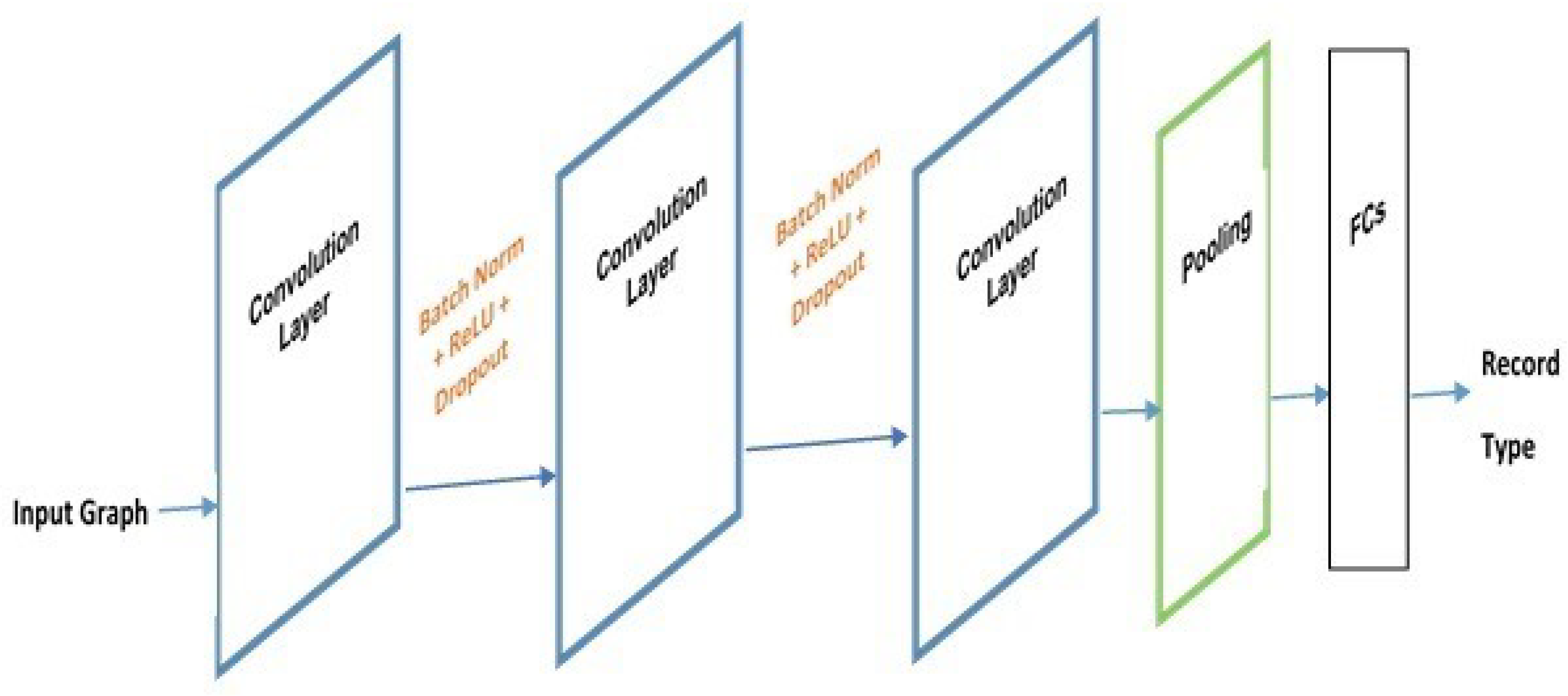This method is summarized in Figure 3. In contrast to fixed-length sequence models, the graph representation naturally captures ECG records of varying durations without resampling. The learned embedding features serve as node features in the GCN. We searched for an optimal GCN architecture. To accomplish this task, we tried several architectures. The first architecture is composed of three convolutional layers, a mean-pooling layer, and two fully connected layers. The convolution layers learn feature embeddings by updating node representations based on aggregated information from neighbors. As a result, at the end, each beat representation is captured by the surrounding beats. After each convolutional layer, we added batch normalization and dropout to stabilize training and reduce the risk of overfitting. We use simple average pooling to reduce the graph to a simpler representation and to transfer node features into a single vector. Thus, the record is summarized by the average beat embedding, followed by two fully connected layers at the end of the GCN. The first layer performs a nonlinear transformation to discriminate features, followed by dropout regularization. The second layer classifies the record using a log-softmax function. The architecture of the proposed GCN is shown in Figure 4.

In the fifth experiment, we reduced the 17-feature matrix to 4 principal components using PCA. This PCA-reduced vector is then fused with the intra-beat GCN embedding of the same heartbeat (Section 3.5, Equations (2)–(5) to form the node representation fed into the proposed inter-beat GCN.

3.5. Two-Level Graph Representation for ECG Record Classification

In the fifth experiment, a graph-based hierarchical learning approach is used to learn about ECG signals at two levels. These include intra-beat modeling of the morphological structure of the heartbeats and inter-beat modeling of the relationship between successive heartbeats in the ECG signal. The entire architecture is shown in Figure 5.

In each ECG record, R-peaks were first identified, and each heartbeat was segmented. Each heartbeat corresponds to a 17-dimensional manually crafted feature vector, comprising 11 time-domain features and 6 frequency-domain features. Principal Component Analysis is used to reduce this feature vector to 4 principal components while retaining 96.3% of its variance. This four-dimensional feature vector is then attached to that particular heartbeat and acts as the node representation of the inter-beat graph. Here, each node corresponds to a heartbeat, and the edges connecting them represent the temporal order of the heartbeats. In addition, the distance (RR interval) between consecutive heartbeats is considered an additional feature of the edge, thereby allowing the graph to contain information not only about heartbeat morphology but also about interbeat variability.

A second GCN layer acts on this inter-beat graph to learn relationships among successive heartbeats. The network aggregates information contained in the PCA-reduced heartbeat feature vectors together with the temporal relationships encoded by the graph edges. As the final step, a pooling layer extracts the representation of the entire ECG recording from the graph convolution results, which is then used to classify the recording with a fully connected classification layer and the softmax activation function.

The introduced model adopts the genuine hierarchy of graph learning, in which the representations learned by the intra-beat graph convolutional network (GCN) are transferred to the inter-beat graph. More specifically, the intra-beat GCN encodes the local morphological features of each ECG beat. Subsequently, the encoded beat representation is combined with the reduced physiological feature vector for the same ECG beat and used as the node representation in the inter-beat graph.

The intra-beat representation of the i-th ECG beat is first learned by the intra-beat GCN as

$${\mathbf{h}}_i^{\mathrm{intra}}={\mathrm{GCN}}_{\mathrm{intra}}({\mathbf{X}}_i,{\mathbf{A}}_i),$$

(2)

where ${\mathbf{X}}_i$ and ${\mathbf{A}}_i$ denote the node feature matrix and adjacency matrix of the intra-beat graph, respectively.

To construct the inter-beat graph, the learned intra-beat embedding is concatenated with the PCA-reduced physiological feature vector,

$${\mathbf{x}}_i=\left[{\mathbf{h}}_i^{\mathrm{intra}}\parallel {\mathbf{p}}_i\right]\in {\mathbb{R}}^{16},$$

(3)

where ${\mathbf{p}}_i$ denotes the reduced physiological feature vector and ‖ represents vector concatenation.

The fused feature vector is subsequently projected into a compact latent representation using a learnable two-layer multilayer perceptron (MLP),

$${\mathbf{z}}_i=\varphi \left({\mathbf{x}}_i\right),$$

(4)

where the projection function is defined as

$$\varphi \left(\mathbf{x}\right)={\mathbf{W}}_2\sigma \left({\mathbf{W}}_1\mathbf{x}+{\mathbf{b}}_1\right)+{\mathbf{b}}_2,$$

(5)

with ${\mathbf{W}}_1\in {\mathbb{R}}^{8\times 16}$, ${\mathbf{b}}_1\in {\mathbb{R}}^8$, ${\mathbf{W}}_2\in {\mathbb{R}}^{4\times 8}$, and ${\mathbf{b}}_2\in {\mathbb{R}}^4$. The hidden layer employs the Rectified Linear Unit (ReLU) activation function,

$$\sigma \left(x\right)=max(0,x),$$

(6)

while no activation function is applied after the final projection layer. Consequently, the 16-dimensional fused feature vector is mapped to a 4-dimensional latent representation that serves as the node feature for the inter-beat graph.

The projected embeddings of all beats are stacked to form the inter-beat node feature matrix,

$$\mathbf{Z}={\left[{\mathbf{z}}_1,{\mathbf{z}}_2,\dots ,{\mathbf{z}}_N\right]}^{\top },$$

(7)

which is subsequently processed by the inter-beat graph convolutional network,

$${\mathbf{H}}^{\mathrm{inter}}={\mathrm{GCN}}_{\mathrm{inter}}(\mathbf{Z},{\mathbf{A}}_{\mathrm{inter}}),$$

(8)

where ${\mathbf{A}}_{\mathrm{inter}}$ denotes the adjacency matrix of the inter-beat graph.

This hierarchical information flow enables the proposed model to progressively capture fine-grained morphological characteristics at the intra-beat level and higher-level temporal relationships among beats at the inter-beat level.

The hierarchical framework jointly exploits intra-beat graph representations and PCA-reduced beat descriptors to improve ECG classification accuracy. This hierarchical training approach makes it possible for the proposed framework to utilize information available at two different levels.

Table 4. Summary of the experimental configurations.

Exp.	Graph Representation	Node Feature Representation
1	Heartbeat graph with five nodes (P–Q–R–S–T) connected in a ring topology	G1: Band power, dominant frequency, and spectral entropy for each ECG wave.
2	Heartbeat graph with five nodes (P–Q–R–S–T) connected in a ring topology	G2: Amplitude, spectral centroid, spectral bandwidth, and spectral flatness for each ECG wave.
3	Heartbeat graph with five nodes (P–Q–R–S–T) connected in a ring topology	G3: Amplitude and temporal offset relative to the R-peak for each ECG wave.
4	ECG record represented as a temporal graph whose nodes correspond to heartbeats connected according to their temporal order	Each beat is initially represented by a 17-dimensional handcrafted feature vector (11 time-domain and 6 frequency-domain features). Two MLPs independently embed the time-domain and frequency-domain features, and the resulting embeddings are concatenated to form the node representation used by the GCN.
5	Same temporal graph representation as Experiment 4	The same 17-dimensional handcrafted feature vector is reduced to four principal components via PCA to form ${\mathbf{p}}_i$. Each heartbeat’s node representation for the inter-beat GCN is the fused vector ${\mathbf{z}}_i=\varphi \left(\left[{\mathbf{h}}_i^{\mathrm{intra}}\parallel {\mathbf{p}}_i\right]\right)$ (Equations (2)–(5)), where ${\mathbf{h}}_i^{\mathrm{intra}}$ is the intra-beat GCN embedding of the same heartbeat and $\varphi$ is the two-layer projection MLP defined in Section 3.5.

shows a summary of the experimental configurations.

3.6. Hyperparameters

The optimization was carried out using the Adam optimizer, with the initial learning rate set to 0.003 and the weight decay coefficient set to ${10}^{-3}$. Training was performed with a batch size of 16 for up to 40 epochs. For increased numerical stability, gradient clipping with a maximum norm equal to 2.0 was used. To control the learning rate, the ReduceLROnPlateau learning schedule was employed, in which the learning rate is halved after three consecutive epochs in which validation accuracy does not increase. The training process would stop after eight consecutive epochs of no improvements in validation accuracy; at that point, the state achieving the best validation accuracy would be retained.

To ensure reproducibility, the random seed was set to 42.

4. Results and Discussion

In this study, we conducted several experiments to determine the best structure to represent the ECG signal and beats. The experiments involved several graph configurations to classify both the ECG signal and individual beats. This section introduces these experiments and evaluates the performance of different graph representations.

Table 5. Summary of the experimental protocol.

Exp.	Task	Training Set	Test Set	Unit
1	Beat-level classification (G1)	20,000 beats extracted from the PTBDB dataset	4029 beats extracted from MIT-BIH records	Beats
2	Beat-level classification (G2)	20,000 beats extracted from the PTBDB dataset	4029 beats extracted from MIT-BIH records	Beats
3	Beat-level classification (G3)	20,000 beats extracted from the PTBDB dataset	4029 beats extracted from MIT-BIH records	Beats
4	Record-level classification	1024 ECG segments from the PTBDB dataset	398 ECG segments from MIT-BIH records	Segments
5	Cross-dataset hierarchical graph classification	1024 ECG segments from the PTBDB dataset	398 ECG segments from MIT-BIH records	Segments

shows the data used in different experiments. In Experiments 1–3, the classifier was trained on 20,000 heartbeat sequences from PTBDB and tested on 4029 heartbeat sequences from the independent MIT-BIH Arrhythmia Database. The goal of this external test is to assess the robustness and generalization of the intra-beat graph representation.

The first experiments performed beat-level classification using GCN, where each graph contains five nodes representing P, Q, R, S, and T, and each node has three features (dominant frequency (Hz), spectral entropy, and band power in the 0–40 Hz band) corresponding to a beat. This approach enables the model to use the features of the ECG waves that have the highest discriminative effect while minimizing the impact of all other nodes. Thus, the resulting graph representation preserves the most important physiological features of each heartbeat.

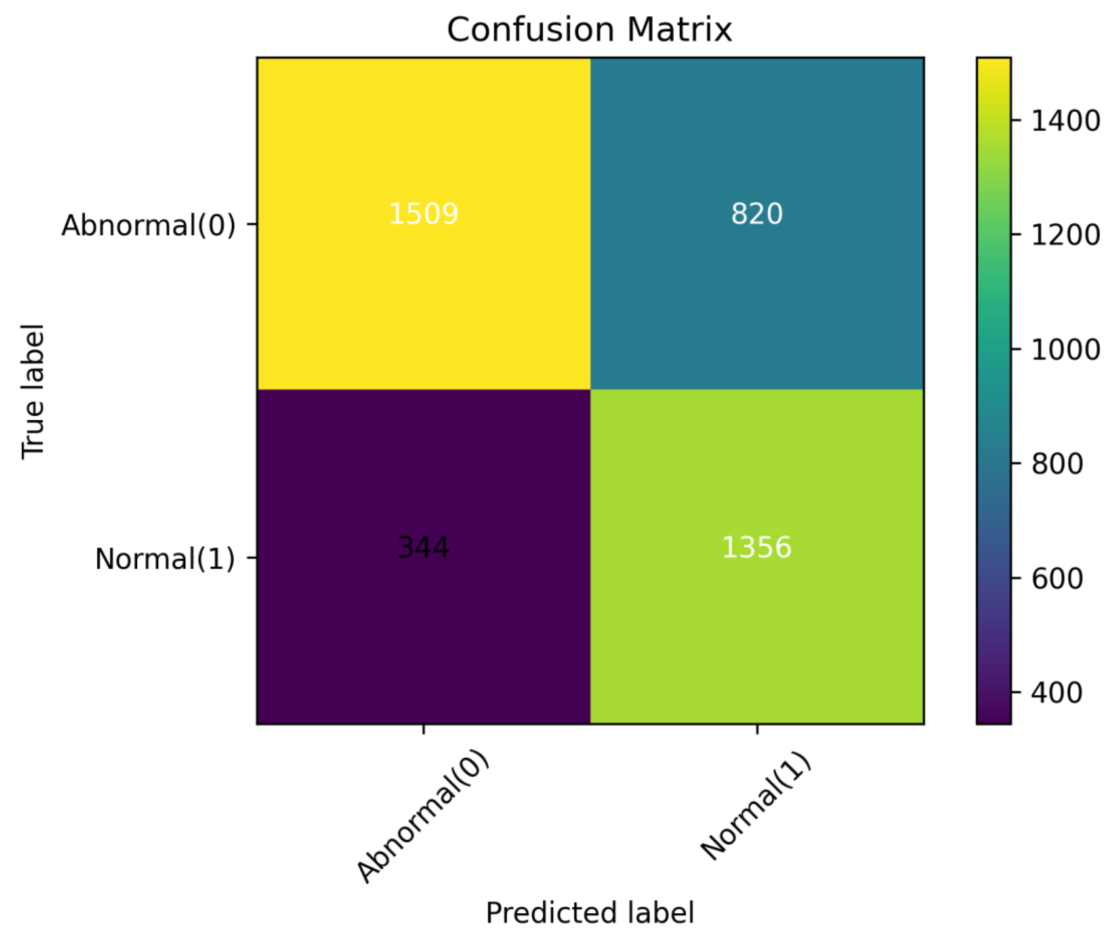
The confusion matrix for dataset 1 is shown in Figure 6. It displays a strong indicator of distinction between normal and abnormal beats. Out of 2329 abnormal beats, 1509 were correctly classified as abnormal, while 820 were incorrectly predicted as normal. For the normal class, 1356 out of 1700 beats were correctly identified, whereas 344 normal beats were falsely classified as abnormal. 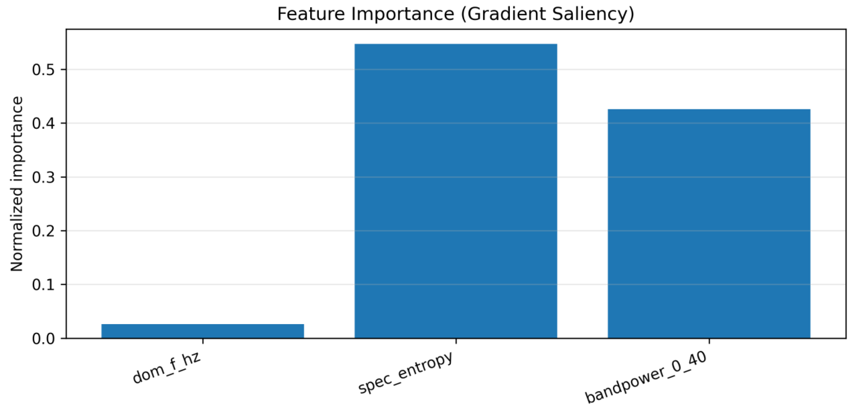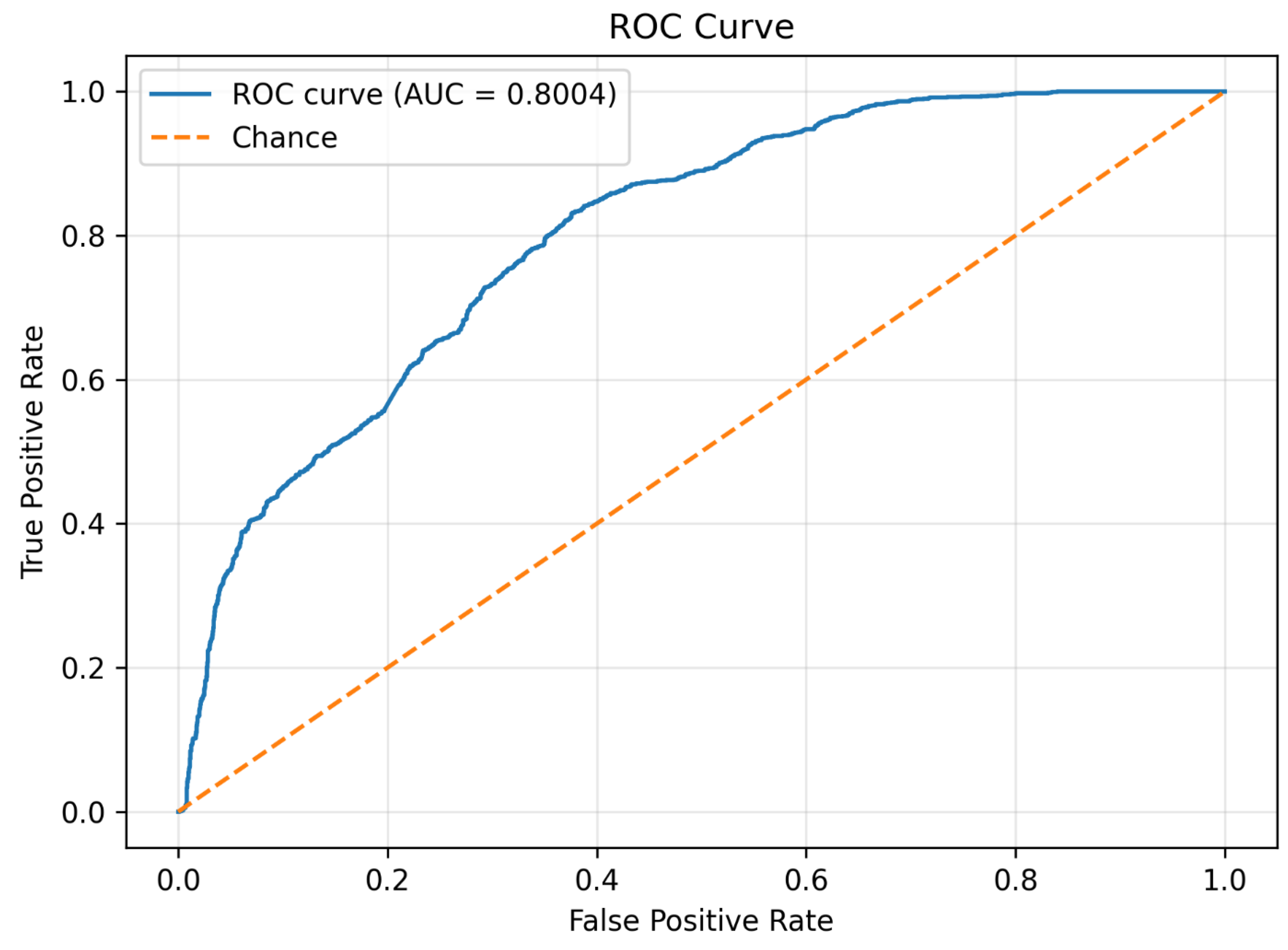A feature importance plot, as indicated in Figure 7, shows how each input feature affects the model’s classification decisions. The plot emphasizes which features are the most important. The importance values are scaled so that they sum to 100 percent. Higher bars in the plot indicate that the feature has a greater impact on the classification decisions. As can be seen, spectral entropy is the most significant feature, accounting for more than half of the total importance in classification decisions, which strongly indicates that model performance depends on frequency components. Band power in the 0–40 Hz range is the second-most significant feature influencing classification decisions. The dominant frequency feature has the lowest effect on classification decisions. The importance plot highlights the critical role of frequency-domain complexity in ECG beat classification. The ROC curve of the model, shown in Figure 8, has an AUC of 0.80, indicating an acceptable predictive rate. The recall, F1-score, and support of the model are evaluated and presented in

Table 6. The Performance of the three experiments.

Class	Precision	Recall	F1-Score	Support
G1
Normal Beats	0.62	0.79	0.69	1700
Abnormal Beats	0.81	0.64	0.72	2329
Macro Average	0.71	0.72	0.71	4029
Weighted Average	0.73	0.71	0.71	4029
G2
Normal Beats	0.88	0.88	0.88	1700
Abnormal Beats	0.91	0.91	0.91	2329
Macro Average	0.90	0.90	0.90	4029
Weighted Average	0.90	0.90	0.90	4029
G3
Normal Beats	0.98	0.78	0.87	1700
Abnormal Beats	0.86	0.99	0.92	2329
Macro Average	0.92	0.88	0.89	4029
Weighted Average	0.91	0.90	0.90	4029

. The model achieves a precision of 0.814, a recall of 0.648, and an F1 score of 0.722 for abnormal beats. For normal beats, the model achieves higher recall and lower precision. The macro-average for both classes illustrates that the model performs similarly across both classes without bias toward one class over the other.

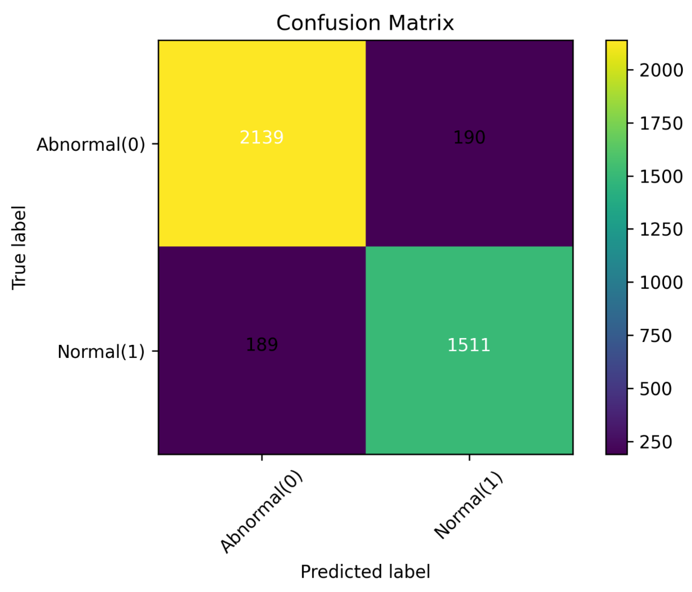
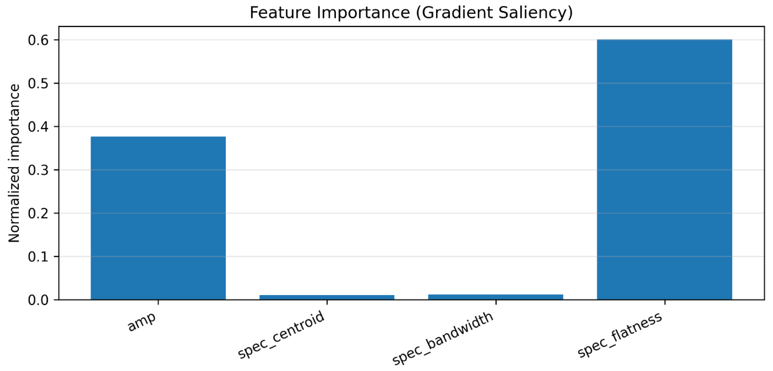
The second Experiment involved a GCN with four features: amplitude (Amp), spectral centroid (spec_centroid), spectral bandwidth (spec_bandwidth), and spectral flatness (spec_flatness). The confusion matrix of this experiment is seen in Figure 9 and indicates robust and balanced predictive performance. Spectral flatness is the most important feature in the classification process; the amplitude feature is the second-most influential. 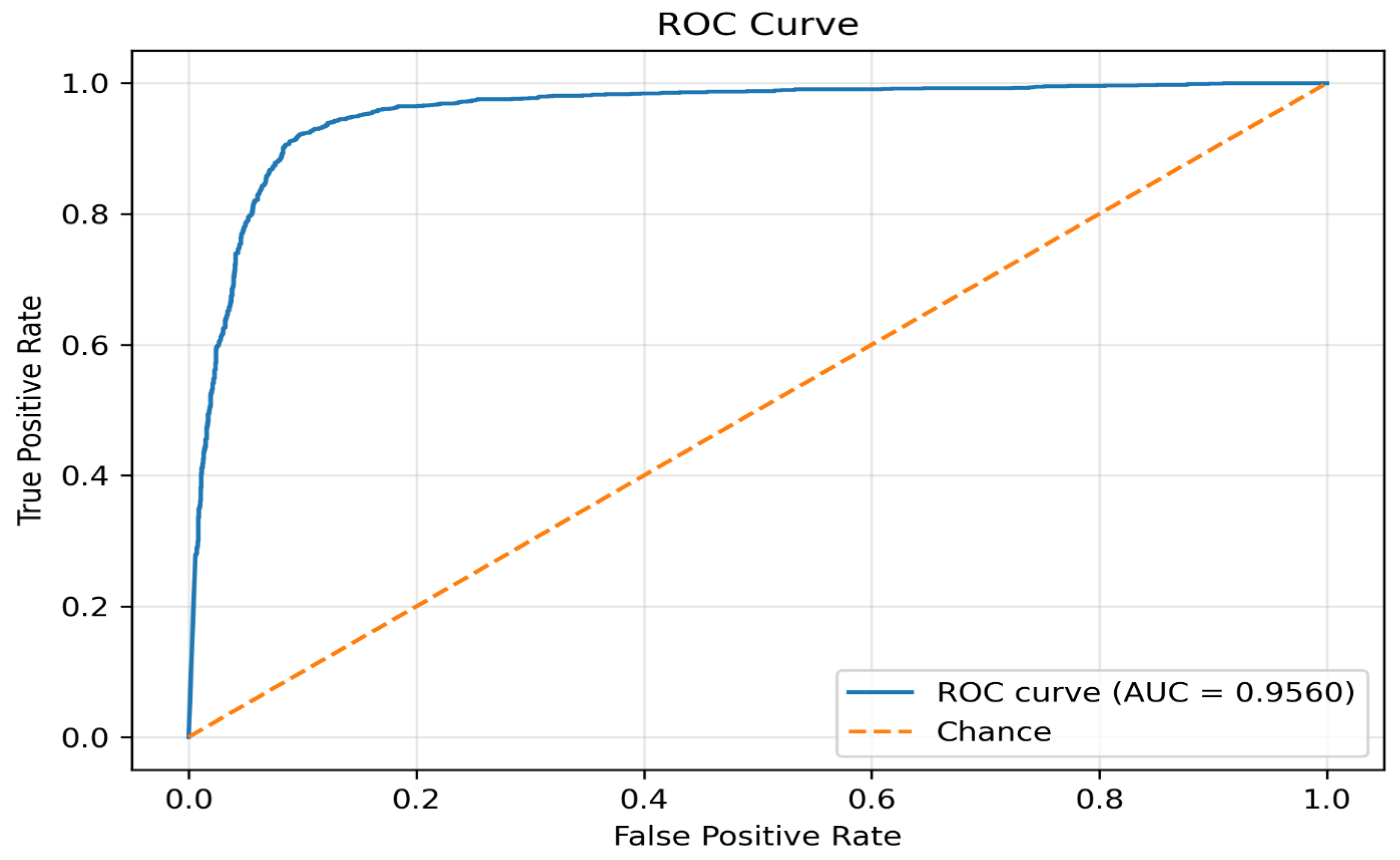Spectral centroid and spectral bandwidth have a low impact on the model’s output, as indicated in Figure 10. The Area Under the Curve (AUC ≈ 0.956), as seen in Figure 11, indicates good performance, demonstrating that the model performs well in distinguishing normal from abnormal beats. The curve indicates that the classifier performs accurately and maintains a stable confidence between sensitivity and specificity.

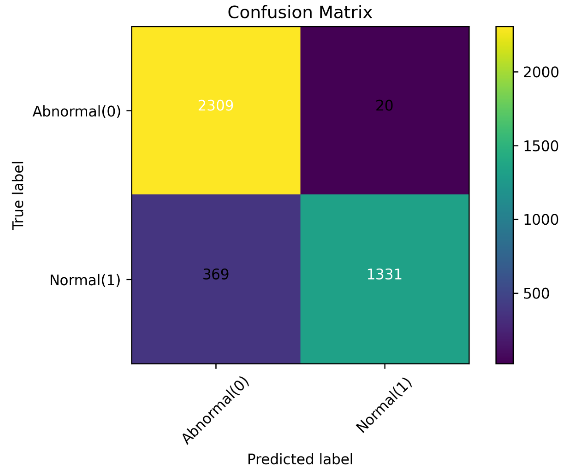
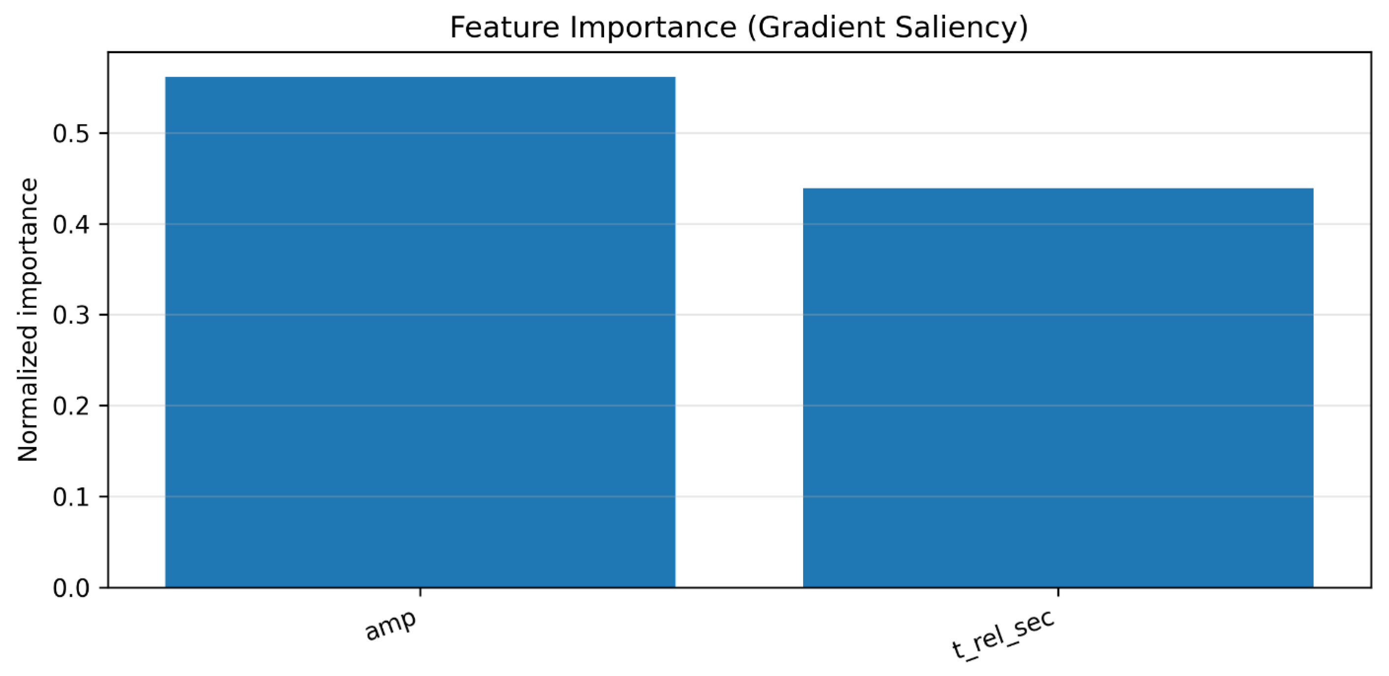
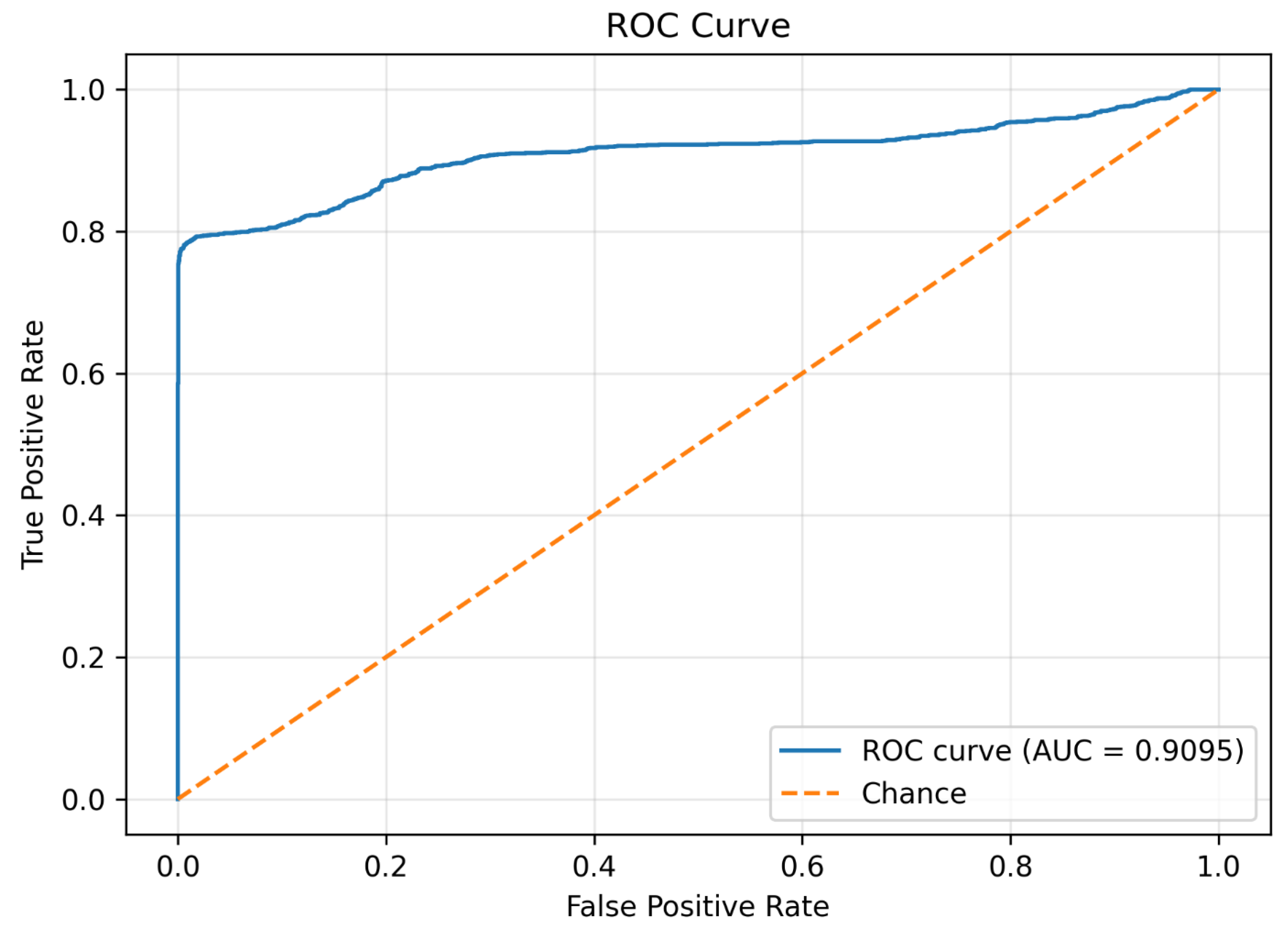
The third Experiment contains two features per node: the amplitude (amp) and the relative time feature (t_rel_sec). The confusion matrix of this experiment is represented in Figure 12. The amp has the greatest influence on the model. In addition, t_rel_sec contributes to model performance, indicating that the temporal positioning of the signal plays an effective role as seen in Figure 13. The relatively close values indicate that the model uses both signal strength and timing information equitably. The model’s ROC curve shows high sensitivity with relatively low false-positive rates. The Area Under the Curve (AUC ≈ 0.91) in Figure 14 indicates good overall performance. The confusion matrix shows that the model could accurately identify abnormal and normal beats.

A comparison of the conducted experiments reveals that the second experiment with a GCN, where each node has four features—Amplitude, Spectral Centroid, Spectral Bandwidth, and Spectral Flatness—demonstrates balanced performance for normal and abnormal beats and has the highest precision and recall for both, implying robust classification. These features provide the GCN with morphological information about beats, facilitating discrimination between the two classes. Experiment 1 shows good performance, with a weighted F1 score of 0.71 and better recall for normal beats than for abnormal beats. Experiment 3 also achieves a high weighted F1 score of 0.90 but shows bias toward abnormal beats. Table 6 summarizes the results of the experiments.

4.1. Comparison with an MLP Baseline

To evaluate whether the graph structure of the intra-beat GCN provides an advantage over a simpler architecture operating on the same information, we trained an MLP classifier on the identical G2 feature set (amplitude, spectral centroid, spectral bandwidth, spectral flatness for each of the P, Q, R, S, and T nodes), concatenated into a single 20-dimensional vector rather than structured as a graph. The MLP was trained and evaluated on the same beat-level split used in experiments 1–3 (20,000 PTBDB training beats, 4029 MIT-BIH test beats). The architecture of the MLP is presented in

Table 7. Architecture of the MLP baseline used to test the necessity of graph convolution on the 5-node intra-beat graph.

Layer	Configuration
Input	20-dimensional concatenated node feature vector
	(G2 features × P, Q, R, S, T)
FC + BN + ReLU + Dropout	$20\to 32$, dropout = 0.3
FC + ReLU + Dropout	$32\to 16$, dropout = 0.3
FC + Log-Softmax	$16\to 2$

BN: batch normalization; FC: fully connected layer.

. The MLP baseline achieved 89.10% accuracy and an F1-score of 0.8800, slightly below the intra-beat GCN’s 90.59% accuracy and 0.9059 F1-score. This indicates a consistent, direction-favorable margin for the graph-based representation.

4.2. Segment-Level Experiments

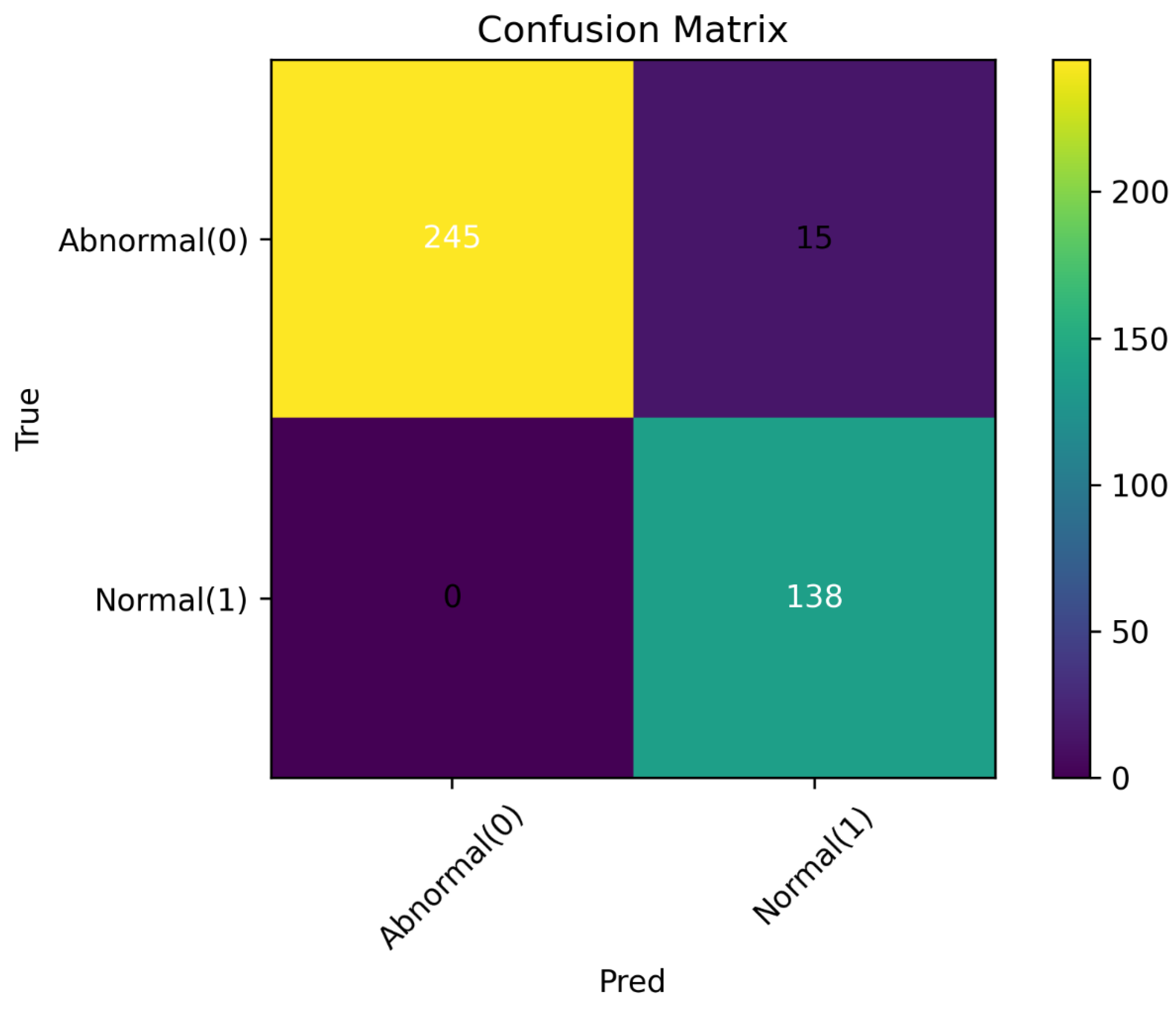
The fourth experiment performs segment classification, where each beat represents a single node. Unlike the previous experiments, which evaluated the proposed framework at the beat level, Experiment 4 performs classification at the ECG segment level. In this setting, each complete ECG segment is represented as a single graph and treated as one sample for classification. The graph construction maintains beat-to-beat reliance while enabling the GCN to aggregate information across beats. Two MLPs are used to learn embedding features that act as node features in the GCN. 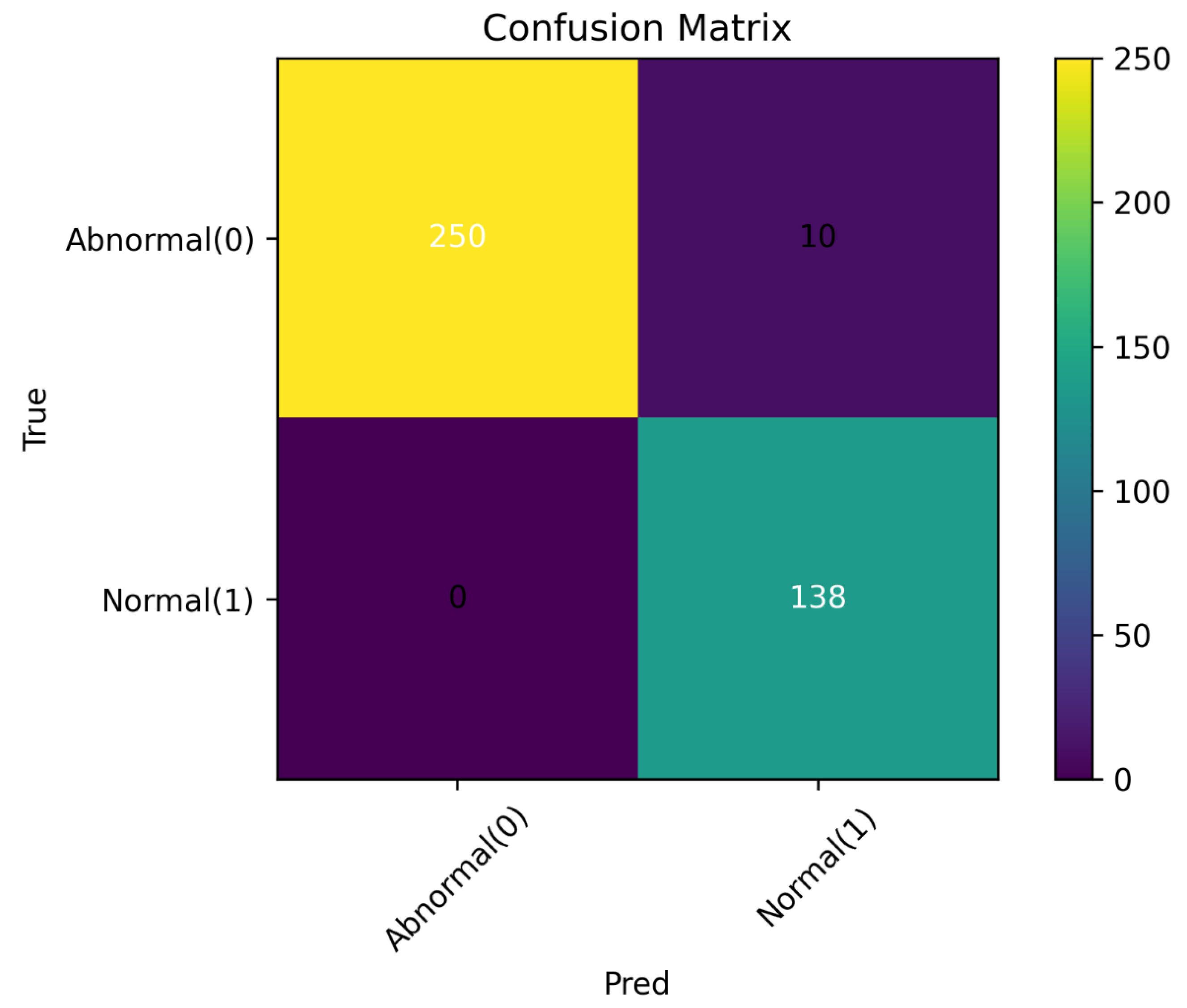The confusion matrix in Figure 15 shows the confusion matrix for Experiment 4. Of the 260 abnormal ECG records, 245 were correctly detected as abnormal, while the remaining 15 were incorrectly detected as normal, resulting in a recall of 94.23% for the abnormal class.

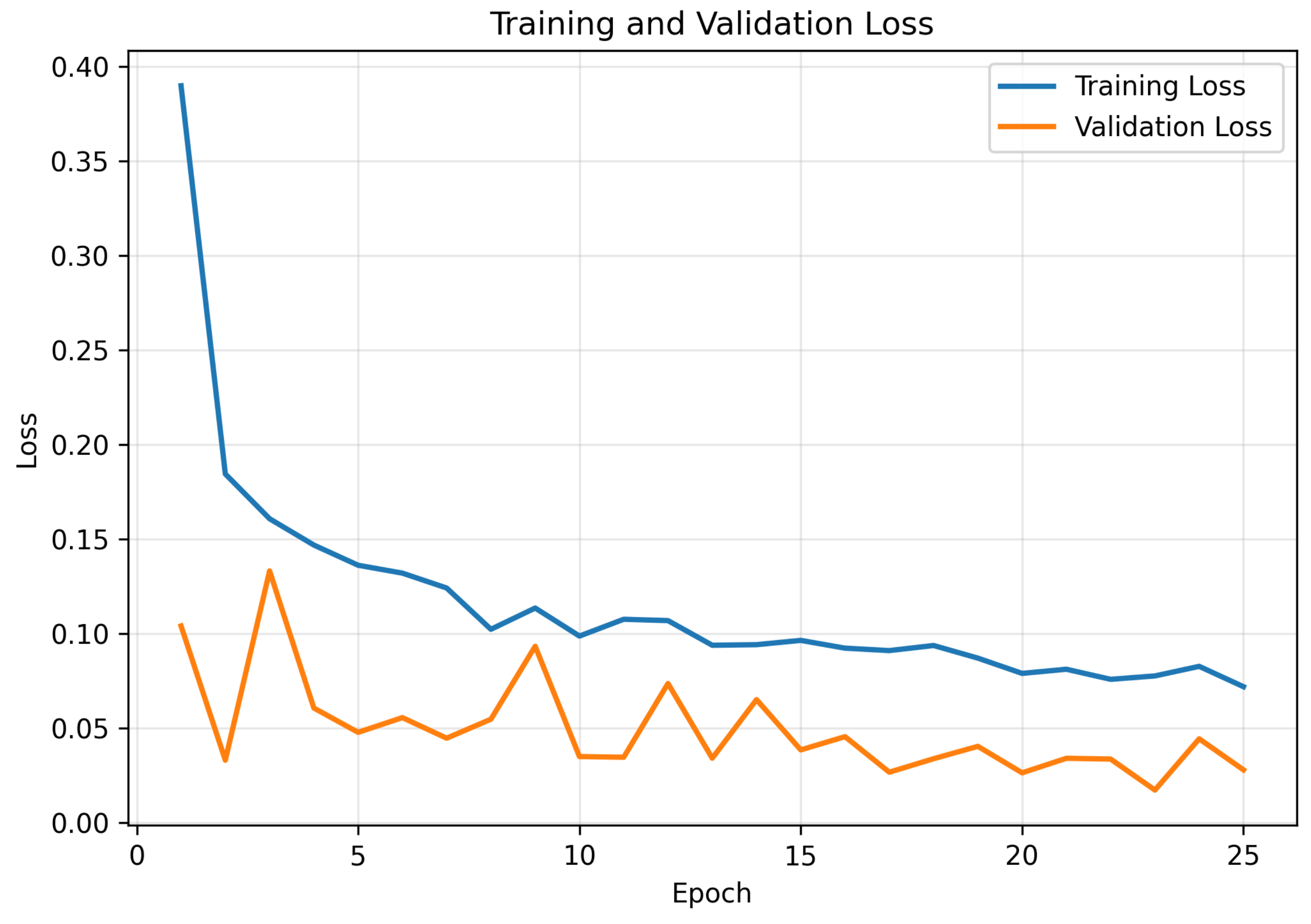
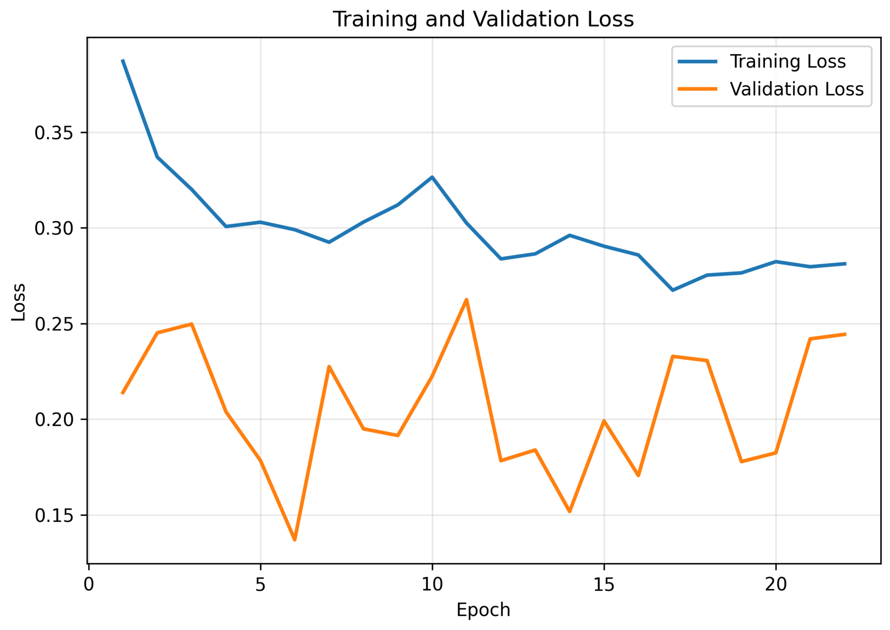
On the other hand, of the 138 normal ECG records, all were correctly detected with no false negatives, resulting in a perfect recall of 100% for the normal class. Therefore, there are no classification errors in the normal class, which implies that the model is quite capable of recognizing the pattern of a normal heartbeat, but the fewer records in the abnormal class indicate that only some of the abnormal data are difficult to classify. Overall, from the analysis using the confusion matrix, it is evident that the inter-beat graph convolutional neural network model can classify normal and abnormal ECG segments accurately, with 15 errors in 398 readings. The suggested model in this experiment achieves an accuracy of 96.23% in classifying ECG segments, which proves the effectiveness of the conducted procedure in maintaining discriminative features for classifying normal and abnormal records, where the model generalizes to learn better representations and thus reduces the risk of overfitting; in addition, it maintains both the beat’s morphology and spectral content. The model’s training loss curve is shown in Figure 16. It demonstrates rapid convergence during the first epochs, which emphasizes the model’s ability to capture dominant signal patterns during these epochs. Then, fine-grained optimization of the learned representation is obtained through a gradual reduction in loss in the final epochs. Training loss stabilizes by the final epochs. The classification results indicate that the model has excellent performance on both normal and abnormal classes. Records from the normal class have a recall level of 1.00, while the abnormal beats have a perfect precision rate. The very high F1 scores across the classes indicate even performance without any bias.

Table 8. Classification report for the proposed model.

Class	Precision	Recall	F1-Score	Support
Normal	0.90	1.00	0.94	138
Abnormal	1.00	0.94	0.97	260
Macro Average	0.95	0.97	0.95	398
Weighted Average	0.96	0.96	0.96	398

summarizes the results of the experiment.

The fifth experiment involves a dual representation for ECG segment classification, in which each record is represented as a temporal graph with one node per heartbeat and edges connecting consecutive beats. Each node’s feature vector is the fused representation ${\mathbf{z}}_i=\varphi \left(\left[{\mathbf{h}}_i^{\mathrm{intra}}\parallel {\mathbf{p}}_i\right]\right)$ described in Section 3.5, combining the intra-beat GCN embedding with the PCA-reduced physiological features; the RR interval between consecutive beats is used as an edge feature; the confusion matrix in Figure 17 indicates an accuracy of 97.49%. Figure 18 presents the loss curve for Experiment 5. The convergence occurs effectively throughout the optimization process. There is a significant decrease in the loss value at the beginning of training due to rapid parameter adaptation and effective gradient-based learning. However, as the process proceeds, the loss gradually decreases; this means that the process of convergence is almost complete. Minor oscillations in later epochs are small and do not affect the overall convergence trend. Thus, the obtained plateau signifies the insignificance of further iterations, meaning that the number of training epochs is sufficient.

Classification results for Experiment 5 are listed in

Table 9. Classification report of the proposed two-level model (Experiment 5).

Class	Precision	Recall	F1-Score	Support
Normal	0.93	1.00	0.96	138
Abnormal	1.00	0.96	0.98	260
Macro Average	0.96	0.98	0.97	398
Weighted Average	0.97	0.97	0.97	398

. Our model achieved an F1 score of 97.51% and an accuracy of 97.49%. It shows good performance for both classes, as it recognized all normal cases with a recall of 100% and a precision of 93.24%. At the same time, it had precision of 100% for the abnormal class, which means that all predicted abnormal cases were correctly recognized, and its recall is 96.15% with an F1 score equal to 98.04%. Macro-averaged precision, recall, and F1-score were 96.62%, 98.08%, and 97.27%, respectively. Also, weighted averages remained high, demonstrating once again that the proposed approach yields proper feature representation and heartbeat embeddings.

To evaluate the stability of the proposed models with respect to the random training process, Experiments 4 and 5 were independently reproduced using five distinct random seeds. The averages and standard deviations for the accuracy, precision, recall, and F1-score for each experiment were computed.

Table 10. Multi-seed stability analysis of the proposed graph-based models over five independent runs using different random seeds. Results are reported as the mean ± standard deviation (%), demonstrating the robustness of the models against random initialization and stochastic optimization.

Experiment	Accuracy	Precision	Recall	F1-Score
Experiment 4	96.39 ± 0.13	95.56 ± 0.82	96.14 ± 0.80	95.28 ± 0.37
Experiment 5	97.67 ± 0.24	96.55 ± 0.41	98.34 ± 0.11	97.18 ± 0.55

presents small standard deviations for all metrics, suggesting stable and replicable results, proving the high stability and replicability of the results produced by the proposed graph-based framework with respect to various initializations of the parameters, mini-batches, and optimizations. Experiment 5 performs slightly better than Experiment 4 but shows the same degree of stability. The standard deviations are less than 1% for all metrics analyzed, indicating that the differences are attributable solely to the proposed method.

4.3. Ablation Study

The objective of the ablation study is to evaluate the contribution of each component of the proposed two-level framework. Three model configurations were compared.

1.

Inter-Beat GCN Only. Each ECG record is modeled as a single temporal graph in which nodes represent heartbeats and edges represent temporal adjacency between consecutive beats.

2.

Intra-Beat GCN Only. Each heartbeat is modeled independently as a five-node P–Q–R–S–T ring graph; no inter-beat edges or temporal relationships between beats are modeled. Among the three intra-beat node-feature configurations (G1, G2, G3), G2 (amplitude, spectral centroid, spectral bandwidth, spectral flatness) achieved the strongest and most balanced performance and is therefore used as the representative intra-beat-only configuration. To enable a fair comparison with the segment-level Inter-Beat GCN Only and Full Proposed Model configurations, beat-level predictions from this model were aggregated to the segment level. For each of the 398 MIT-BIH test segments, the trained model’s predictions on all constituent beats were combined using the same rule used to construct the ground-truth segment labels (Section 3.2): a segment was predicted abnormal if one or more of its constituent beats was predicted abnormal, and predicted normal otherwise. This yields a segment-level accuracy and F1-score for the Intra-Beat-Only configuration that is directly comparable to the other two configurations, both of which operate natively on 398 segments.

3.

Full Proposed Model. The complete two-level hierarchical architecture, combining the intra-beat P–Q–R–S–T graph with the PCA-reduced inter-beat temporal graph.

Table 11. Ablation study of the proposed framework.

Model	Corresponds to	Accuracy (%)	F1-Score
Inter-Beat GCN Only	Experiment 4	96.23	0.9627
Intra-Beat GCN Only	Experiment 2 (segment-aggregated)	89.44	0.9010
Full Proposed Model	Experiment 5	97.49	0.9751

reports accuracy and weighted F1-score for each configuration, evaluated uniformly at the segment level (n = 398) to ensure direct comparability.

The results confirm that both the inter-beat and intra-beat representations individually contribute useful information for ECG classification and that combining them in the full two-level hierarchical model yields the best performance on both accuracy and F1-score. Notably, the inter-beat-only configuration outperforms the intra-beat-only configuration in this comparison, which is consistent with rhythm-level information across multiple beats being more discriminative for record-level (as opposed to individual beat-level) classification of normal versus abnormal ECG segments. While Table 11 reports single-run results on the fixed 398-segment test set, the multi-seed results in Table 10 allow this improvement to be tested formally. The paired t-test on the per-seed accuracy and F1-score between the Full Proposed Model (Experiment 5) and the Inter-Beat GCN Only model (Experiment 4) for the same five seeds shows that even a small difference in their point estimates is significant (

Table 12. Paired statistical comparison of the Full Proposed Model (Experiment 5) against Inter-Beat GCN Only (Experiment 4), per-seed accuracy and F1-score, paired t-test, $n=5$ seeds.

Metric	Mean Difference (pp)	t-Statistic	df	p-Value	Significant ($\mathit{\alpha }=0.05$)
Accuracy	1.28	8.83	4	0.0009	Yes
F1-score	1.90	19.42	4	<0.0001	Yes

pp: percentage points; df: degrees of freedom. Experiment 4 (Inter-Beat GCN Only): accuracy $96.39\pm 0.13\%$, F1-score $95.28\pm 0.37$. Experiment 5 (Full Proposed Model): accuracy $97.67\pm 0.24\%$, F1-score $97.18\pm 0.55$ (mean ± standard deviation, $n=5$ seeds; see Table 10).

). There was an increase in accuracy by 1.28 percentage points ($t\left(4\right)=8.83$, $p=0.0009$) and F1-score by 1.90 percentage points ($t\left(4\right)=19.42$, $p<0.0001$), which is much less than $\alpha =0.05$. This suggests that the difference between these models is systematic with respect to random seeds and not just a stochastic one-off result.

4.4. Baseline Architectures

To assess the performance of our hierarchical model relative to baseline architectures, we propose two baselines: a CNN and a single-level GCN that serves as a substitute for prior GCN-based ECG methods. All operate on the same classification unit as Experiments 4 and 5, so they are directly comparable to the proposed two-level model. The architectures of the proposed CNN and GCN baselines are presented in

Table 13. Architecture of the 1D-CNN baseline used for ECG classification.

Layer	Configuration
Conv1D + BN + ReLU + MaxPool	16 filters, kernel size = 7, stride = 1, pool size = 2
Conv1D + BN + ReLU + MaxPool	32 filters, kernel size = 5, stride = 1, pool size = 2
Conv1D + BN + ReLU + GAP	64 filters, kernel size = 3, global average pooling
FC + ReLU + Dropout	$64\to 32$, dropout = 0.3
FC + Log-Softmax	$32\to 2$

BN: batch normalization; GAP: global average pooling; FC: fully connected layer.

and

Table 14. Configuration of the single-level generic ECG-GCN baseline.

Component	Configuration
Nodes	ECG segment divided into 30 equal 60-sample windows, providing a generic temporal decomposition independent of the P/Q/R/S/T landmarks.
Node features	Per-window mean, standard deviation, minimum, maximum, and dominant frequency, resulting in a 5-dimensional generic statistical feature vector for each node.
Edges	Bidirectional sequential-chain edges representing temporal adjacency, augmented with k-nearest-neighbor (k-NN) connections in node-feature space with $k=3$. This provides generic temporal and similarity-based connectivity without imposing the physiological ring topology used in the proposed model.
GCN layers	Two GCNConv layers with dimensions $5\to 32\to 32$, each followed by batch normalization, ReLU activation, and dropout with a rate of 0.3.
Readout	Global mean pooling → FC $(32\to 16)$ → ReLU → Dropout $\left(0.3\right)$ → FC $(16\to 2)$ → Log-Softmax.

GCN: graph convolutional network; FC: fully connected layer; k-NN: k-nearest neighbors.

, respectively. In addition, we used the same training and optimization settings as the proposed two-level model, and the baseline models were trained on the identical 1024 PTBDB segments and tested on the identical 398 MIT-BIH segments.

Table 15. Performance comparison of the baseline models and the proposed hierarchical model.

Model	Accuracy (%)	Recall	F1-Score
1D-CNN	$95.23\pm 0.05$	$96.13\pm 0.66$	$95.00\pm 0.93$
Single-level GCN (generic)	$93.00\pm 0.89$	$92.00\pm 0.34$	$93.63\pm 0.96$
Proposed (two-level hierarchical)	$\mathbf{97}.\mathbf{67}\pm \mathbf{0}.\mathbf{24}$	$\mathbf{98}.\mathbf{34}\pm \mathbf{0}.\mathbf{11}$	$\mathbf{97}.\mathbf{18}\pm \mathbf{0}.\mathbf{55}$

Note: Bold values indicate the Accuracy, Recall, and F1-Score of the proposed method.

presents the performance of all models in terms of accuracy, recall, and F1-score. The proposed two-level hierarchical model achieved the highest F1-score and accuracy among all models, 97.18 ± 0.55% and 97.67 ± 0.24%, respectively, outperforming the CNN by approximately 2 percentage points in accuracy and in F1-score. The single-level GCN baseline, which lacks physiologically structured, hierarchical graph construction, achieved approximately 93% accuracy, supporting the central claim that hierarchical intra-beat/inter-beat structure enhances performance.

The paired t-test was used to compare the per-seed F1-scores of the proposed model with the 1D-CNN and single-level GCN baselines for all five random seeds shown in Table 15.

Table 16. Paired statistical comparison against the proposed model (per-seed F1-score, paired t-test, $n=5$ seeds).

Comparison	Mean F1 Difference (pp)	t-Statistic	df	p-Value	Significant ($\mathit{\alpha }=0.05$)
Proposed vs. 1D-CNN	2.18	10.85	4	0.0004	Yes
Proposed vs. Single-Level GCN	3.55	19.95	4	<0.0001	Yes

pp: percentage points; df: degrees of freedom.

shows the results. The proposed two-level hierarchical model was statistically significantly better than the 1D-CNN baseline (F1-score mean difference of 2.18 percentage points, t(4) = 10.85, p = 0.0004) and single-level GCN baseline (F1-score mean difference of 3.55 percentage points, t(4) = 19.95, p < 0.001).

5. Conclusions

We present a physiologically motivated, two-level graph-based ECG classification method using GCNs. Most prior work follows one of two directions: treating the ECG as a signal sequence with little physiological interpretation, or representing it as a single-level graph that does not separate beat morphology from rhythm. This paper proposes a new representation of ECGs based on intra-beat and inter-beat relationships among physiological markers (P, Q, R, S, and T) within each beat and between beats across the entire segment. In other words, the intra-beat level represents a single heartbeat as a graph where the nodes are made up of the main component parts of a normal heartbeat. In contrast, the inter-beat level represents a series of ECGs as a graph sequence, with relationships between beats represented as edges in the graphs. Three distinct types of node feature combinations were evaluated to ascertain which one offered the highest level of information for classifying electrocardiograms (ECGs). The highest overall classification performance was achieved with the following four measured characteristics: amplitude, spectral centroid, spectral bandwidth, and spectral flatness when combined to form a feature set to classify ECG signal data into one of two groups: normal or abnormal function. The method modeled both shape- and rhythm-based information well, which allowed accurate separation of normal and abnormal beats, enabling accurate distinction between normal and abnormal heart functions.

To evaluate cross-dataset generalization, the proposed network was trained on the PTBDB database and tested on the independent MIT-BIH Arrhythmia Database. The MIT-BIH dataset was not included in any part of the network training process, including but not limited to validation, parameter optimization, feature selection, and model selection. To ensure compatibility between databases, the same preprocessing method was utilized for both, including normalization, beat detection, segmentation, feature extraction, and label adjustment. All network parameters were estimated solely on the training database. The method was validated using data from the PTBDB database for training and the MIT-BIH Arrhythmia Database for testing model performance.

The findings demonstrate that the proposed approach generalizes effectively across datasets from different sources and demonstrated that using dimensional data in the form of dual-layer representations of graphs provided sufficient information about ECG data’s temporal (time-based) and structural (shape-based) relationships. The ablation study, evaluated uniformly at the segment level on the identical 398-segment MIT-BIH test set, confirmed that capturing both intra-beat morphology and inter-beat rhythm gives the best results when predicting ECG diagnosis: the complete proposed system exceeded each of its simplified single-level configurations, and this improvement over the stronger of the two individual components was confirmed as statistically significant across five random seeds.

This work has several limitations: it solves only a binary classification problem, the MIT-BIH database and PTBDB label different types of abnormalities, and fiducials are detected using simple criteria. Future work will extend the method to multi-class arrhythmia classification; add stronger delineation; evaluate broader comparisons with LSTM- and Transformer-based architectures on larger training sets; test on additional databases; and include a within-database control that evaluates normal vs abnormal separation using training and test partitions drawn from a single database, to isolate acquisition-related effects from genuine cross-pathology generalization.