


Abstract
Wind turbine blades endure cyclic loading and variable aerodynamic stresses that make them prone to cracks, requiring early detection for predictive maintenance. This work classifies blade condition into four categories (healthy and with light, intermediate, and severe damage) from triaxial accelerometer signals under rotor speed varying between 0 and 12 rps. Robustness to variable speed is achieved through computed order tracking, using a tachometer signal to re-express vibration signals in the angle domain. From overlapping angle-domain windows, 130 non-redundant time- and frequency-domain descriptors are computed across three accelerometer axes (43 per axis) plus mean rotor speed. A fully nested cross-validation procedure, repeated within each leave-one-trial-out fold to avoid bias, first determines the discriminative axis, then sizes the final feature set to each classifier’s statistical criterion. The search converges on a single axis (Vy), outperforming an unrestricted three-axis search. After redundancy pruning, the random forest retains eight features and the support vector machine thirteen, the former a subset of the latter, reaching 94.9% and 95.2% accuracy; severe damage is recognized with up to 98.4% recall. Regarding the features, mean rotor speed is retained by both classifiers, indicating that order tracking mitigates, but does not completely eliminate, speed dependence. Moreover, severely damaged blades operate at lower speed than other conditions (Kruskal-Wallis, ), suggesting that rotor speed itself provides a genuine damage signature.
1. Introduction
Wind turbines have an important role in the transition toward renewable energy sources, and their installed capacity continues to grow gradually worldwide as part of decarbonization strategies for the electricity sector [1,2]. Among their components, blades are particularly critical: they are continuously subjected to cyclic loads, variable aerodynamic stresses, and adverse environmental conditions, making them prone to developing structural defects such as cracks [3,4]. An undetected crack can progressively propagate until it causes catastrophic blade failure, compromising installation safety, drastically increasing corrective maintenance costs, and causing unplanned downtime that reduces turbine availability and profitability [3,4,5]. Reliable methods for early detection and severity classification of blade damage are therefore essential for an effective predictive maintenance strategy.
In recent years, several studies have addressed the detection and classification of wind turbine blade damage through vibration signal analysis combined with machine learning algorithms. Rangel-Rodriguez et al. [6] analyzed vibration signals from a low-power wind turbine under different damage conditions (healthy, light, intermediate, and severe) and different wind speeds, using statistical and harmonic indices as features, ANOVA-based feature selection, and k-nearest neighbors classification, compared against neural networks, decision trees, and support vector machines. The same authors later proposed a complementary approach based on empirical mode decomposition (EMD) of the vibration signal and convolutional neural networks (CNNs), transforming the signal into time-frequency representations for classification [7]. Sevilla-Camacho and Robles-Ocampo [8] proposed locating cracks in low-power wind turbine blades using a single piezoelectric accelerometer and a support vector machine, achieving over 99% accuracy with a reduced dataset. Ogaili et al. [9] proposed a methodological framework for detecting multiple faults (cracks at different blade locations) using feature-ranking techniques (ReliefF, chi-square, information gain) and several supervised classifiers, including random forests. Korolis et al. [10] evaluated damage diagnosis in a lab-scale floating wind turbine model under different wind speeds and directions, using classification methods based on multiple models, k-nearest neighbors, and support vector machines, highlighting the importance of diagnostic methods being robust to changing operating conditions. More recent studies have further investigated vibration-based and learning-based approaches for wind turbine blade condition monitoring. Sethi et al. [11] combined vibration signals, continuous wavelet transform, and convolutional neural networks for the diagnosis of different blade fault conditions. Rezazadeh et al. [12] investigated dimensionality-reduction techniques for representing and classifying damaged wind turbine blades using vibration-based structural health monitoring. Aranizadeh et al. [13] proposed a failure detection methodology for small-scale wind turbine blades based on monitored data obtained from accelerometers and strain gauges. Pan et al. [14] developed a deep learning-based fault detection approach using graph Fourier transform and acoustic signals. Ma et al. [15] proposed a hybrid 1D-CNN-BiLSTM-AdaBoost architecture combined with multi-source data fusion for wind turbine blade fault diagnosis.
Two broad families of approaches can be distinguished in these studies. Deep learning models, such as the CNN, CNN-LSTM, and hybrid architectures reported in [7,11,14,15], learn discriminative representations directly from raw vibration signals or from their time–frequency transforms, avoiding manual feature engineering and frequently reaching very high accuracy. However, they typically require large labeled datasets, which are costly to obtain for damaged blades; they are prone to overfitting when trained on small, laboratory-scale datasets; they involve many hyperparameters and a considerable computational cost; and they offer limited physical interpretability of their decisions. Approaches based on hand-crafted features combined with classical classifiers [6,8,9,10], in contrast, depend on the quality of the engineered descriptors, but are data-efficient, computationally light, and transparent, since each feature has a direct statistical or physical meaning. The latter approach is adopted in this work for three reasons: (i) the dataset comprises 40 trials, so that, once overlapping windows are grouped by trial to avoid data leakage, the number of independent training units is too small to train a deep network reliably; (ii) interpretability is required to determine which accelerometer axis, which descriptors, and which speed-related effects drive the classification, a central objective of this study; and (iii) a compact feature set and a lightweight classifier are better suited to embedded, real-time deployment in predictive-maintenance systems.
Despite these advances, most reported studies evaluate classifier performance under constant or discrete rotor speed conditions (comparing across a few fixed speeds), without explicitly addressing the case of a rotational speed that varies continuously within a single trial. This limitation is relevant because wind turbines typically operate under dynamic conditions, where fluctuations in wind speed and control actions produce continuous changes in rotor speed, altering the vibration characteristics and introducing patterns that may interfere with damage-related features. In this regard, this work proposes a methodology for the automatic classification of wind turbine blade condition (healthy, and with light, intermediate, and severe damage) from triaxial accelerometer signals, whose distinguishing feature is robustness to rotor rotational speed, which varied continuously between 0 and approximately 12 rps within each trial. This robustness is achieved through computed order tracking: by using a synchronized tachometer signal, the vibration signals are converted from the time domain into the angle domain (revolutions), so that phenomena tied to rotation always appear at the same order regardless of the instantaneous speed. As shown in Section 4.6, order tracking does not remove the dependence of vibration amplitude on speed; this residual dependence is explicitly quantified, and mean rotor speed is retained as an input so that the classifiers can account for it.
The remainder of this article is organized as follows: Section 2 presents the theoretical framework of the concepts used; Section 3 describes the proposed methodology, including data acquisition, order-tracking-based preprocessing, feature extraction and selection, and the classification models used; Section 4 presents the results obtained and their discussion; and finally, Section 5 presents the conclusions of this work.
2. Theoretical Framework
2.1. Vibration-Based Structural Health Monitoring
Vibration-based structural health monitoring (SHM) rests on the principle that a change in the structure’s physical properties (stiffness, mass, damping), such as one produced by a crack, manifests as a measurable shift in its vibrational response [3,12]. In rotating elements like wind turbine blades, these changes typically appear as periodic alterations tied to the rotor’s rotation [6,10]. This tendency motivates analyzing the signal as a function of the rotor’s angular position rather than relying on time alone [16].
2.2. Rotating Machinery Diagnostics Under Variable Speed
If the rotational speed remains constant, standard spectral analysis (using an FFT on the time-domain signal) adequately links frequency components to specific physical phenomena [16,17]. However, under non-stationary operating conditions, like the 0-to-12 rps speed sweep examined in this study, the frequencies associated with a given physical phenomenon shift alongside the instantaneous speed. This variation scatters the signal’s energy across the spectrum, making consistent detection difficult across trials performed at varying speeds [17].
2.3. Order Tracking
Order tracking is the technique that resolves this problem by re-expressing the signal not as a function of time but of the angle rotated by the rotor (in revolutions) [16,17,18]. In this domain, a phenomenon geometrically tied to rotation (e.g., an impact occurring once per revolution) always occupies the same relative position within each revolution. Consequently, the position of rotation-related phenomena in the order domain becomes independent of the rotor’s instantaneous velocity, although their amplitude may still depend on it (Section 4.6) [17,18].
The reason conventional, time-domain spectral analysis fails under these conditions can be stated precisely. For a rotation-synchronous phenomenon of order o (occurring o times per revolution), its instantaneous frequency in Hz is , which changes continuously as the rotor accelerates or decelerates [16,18]. A conventional Fourier transform, computed over a time window spanning a range of speeds, does not see a single frequency component but an entire family of them, one for each instantaneous speed visited during that window; the resulting spectral energy is smeared across the whole frequency band swept by , rather than appearing as a sharp, easily identifiable peak. Because the rotor spends comparatively more time near the turning points of the speed profile (where ) than while sweeping rapidly through intermediate speeds, this smeared energy is also unevenly distributed, often concentrating near the extrema of the swept band; such concentrations can be mistaken for genuine resonances even though they arise purely from the kinematics of the speed profile itself. Order tracking removes this ambiguity by re-expressing the same phenomenon in the angle domain, where its periodicity in is constant, i.e., exactly o cycles per revolution, regardless of how evolved in time, collapsing the smeared band back into a single, sharp peak at order o [16,18]. Figure 1, discussed further below, illustrates this effect on a simulated example.
Figure 1.
Effect of computed order tracking on a simulated signal, , with order-1 and order-2 components under a non-stationary speed profile: (a) simulated time-domain signal, showing the stretching/compression of its instantaneous frequency as speed varies; (b) simulated instantaneous rotor speed; (c) conventional time-domain spectrum, smeared across the frequency bands swept by each order; (d) order-domain spectrum after resampling to the angle domain, showing sharp, speed-invariant peaks at orders 1 and 2.
Two main variants are distinguished: hardware-based order tracking (physical resampling synchronized to encoder pulses) and Computed Order Tracking (COT), which digitally resamples an already-acquired signal using an independently measured instantaneous speed [16,17,18]. This work uses the latter variant, based on a tachometer signal.
Mathematically, if is the instantaneous rotor speed (in revolutions per unit time), the cumulative angle (in revolutions) is obtained by integration:
The original signal, uniformly sampled in time, is then re-interpolated by linear interpolation onto a grid uniformly spaced in , yielding an equivalent signal uniformly sampled in angle, at a fixed resolution of samples per revolution, rather than in time. This angular resolution plays the same role in the angle domain that the sampling rate plays in the time domain: it fixes the highest order that can be resolved without aliasing (the Nyquist order, equal to half the number of samples per revolution), and must therefore be chosen high enough to capture the highest-order phenomenon of interest, analogous to the usual sampling-rate requirement in conventional signal acquisition.
A centrally derived concept is that of order: while frequency (Hz) measures cycles per second, order measures cycles per revolution. An “order 1” (1X) phenomenon occurs once per rotor revolution, “order 2” (2X) twice per revolution, and so on, independent of the absolute rotational speed.
Figure 1 illustrates these effects together on a simulated example, built for clarity rather than reproducing a specific experimental trial: a signal containing an order-1 component (dominant) and an order-2 component (secondary), both phase-locked to the rotor angle, under a smooth, non-stationary speed profile qualitatively similar to the 0-to-12 rps sweep described in Section 3.1 (Figure 1a,b). The time-domain signal itself (Figure 1a) visibly changes character as speed varies: its instantaneous frequency stretches out near the beginning and end of the profile, where the rotor turns slowly, and compresses into a dense, rapidly oscillating waveform near the middle, where speed peaks, i.e., a direct visual signature of the same non-stationarity that spectral smearing exploits. Its conventional, time-domain spectrum (Figure 1c) shows both components smeared across the entire frequency band swept by the corresponding order (shaded regions), with a spurious concentration of energy near the upper edge of each band, exactly as described above, most visibly for order 1, where the smeared energy peaks near the profile’s maximum speed rather than at any single, physically meaningful frequency. After computed order tracking, the same signal’s order-domain spectrum (Figure 1d) resolves both components as sharp, well-defined peaks at orders 1 and 2, independent of the speed profile that generated them.
2.4. Feature Extraction from Vibration Signals
For each window of the signal (already in the angle domain), numerical descriptors, i.e., features, are computed to summarize different aspects of its behavior [6,9]. A direct audit of the feature-extraction implementation (Appendix A) showed that five descriptors originally intended as order-domain-specific, i.e., RMS, skewness, crest factor, peak-to-peak, and kurtosis, are computed by exactly the same formula (kurtosis up to an additive constant) as a time-domain descriptor already present elsewhere in the pipeline; these are reported once, under their time-domain name, throughout this article. With this consolidation, two non-overlapping feature families remain: time-domain and frequency-domain descriptors.
2.4.1. Time-Domain Features
These are computed directly on the angle-domain window and include measures of central tendency and dispersion (mean, standard deviation, square-root amplitude, range/peak-to-peak, mode, median, RMS), distribution shape (skewness, kurtosis, higher-order normalized moments), dimensionless condition factors widely used in vibration diagnostics (crest factor, shape factors, impulse factor, latitude factor, skewness factor, kurtosis factor), and nonlinear complexity and information-theoretic descriptors: the Katz [19] and Higuchi [20] fractal dimensions, which quantify the complexity or roughness of the waveform, and Shannon [21] and Rényi [22] entropy, which quantify, in information-theoretic terms, the degree of uncertainty or disorder in the signal’s instantaneous energy. Mean rotor speed, obtained from the tachometer rather than the accelerometer and computed once per window rather than per axis, is grouped with this family as a physical, time-domain control variable (Section 3.6).
2.4.2. Frequency-Domain Features
These are obtained from the Fast Fourier Transform (FFT) of the window (with Hanning windowing to reduce spectral leakage), re-expressing the frequency axis in order units rather than Hz [16,17]. From the magnitude spectrum , spectral moments (spectral centroid, spectral variance, spectral skewness and kurtosis) and the energy contained within specific order bands (1X, 2X, 3X, 4X, and a higher-order band above 4X), associated with fundamental rotational phenomena and their harmonics, together with the kurtosis of the full order spectrum, were computed.
The complete, non-redundant list of all 43 features computed per accelerometer axis (26 time-domain and 17 frequency-domain descriptors) is provided in Appendix A (Table A1 and Table A2) for completeness and reproducibility; mean rotor speed is listed alongside the time-domain descriptors in Table A1.
2.5. Feature Selection
Because 43 non-redundant features were computed for each accelerometer axis (26 time-domain plus 17 frequency-domain features; Section 2.4), evaluated independently across the three vibration axes (Vx, Vy, Vz), together with mean rotor speed, the initial candidate space comprised 130 descriptors, without any axis being presupposed as more informative than the others. Rather than fixing an arbitrary subset size in advance, a fully nested (doubly cross-validated) selection procedure was used, repeated independently within each fold of the leave-one-trial-out cross-validation scheme (Section 2.6), to avoid the optimistic bias that selecting features on the full dataset before validation would otherwise introduce [11,23]. This procedure was applied in two stages. First, a nested search combining Random Forest importance ranking with a pairwise-correlation redundancy analysis was applied to the full 130-feature space to determine which accelerometer axis carries the discriminative information [13,24]. Second, within the axis identified as informative, a more exhaustive refinement, combining a nested one-standard-error accuracy-versus-feature-count criterion evaluated over the entire candidate range, recursive feature elimination with cross-validation (RFECV) [25], and the same pairwise-correlation redundancy analysis, identified a non-redundant final feature set sized independently for each classifier, reported in Table 1 for the random forest and Table 2 for the SVM (x: acceleration signal window with N samples; : FFT of the window; : mean of x). A between-condition comparison of mean rotor speed, using the Kruskal–Wallis [26] and Mann–Whitney [27] tests, was additionally performed given its role among the final features. The complete procedure, including the validation scheme used to avoid an optimistic bias in the ranking itself, is described in Section 3.6, and its results are presented in Section 4.3 and Section 4.4.
Table 1.
Mathematical definitions of the eight features retained in the final random forest model.
Table 2.
Mathematical definitions of the thirteen features retained in the final SVM model. The first eight (above the mid-rule) are identical to, and listed in the same order as, the random forest’s set in Table 1; the remaining five are used only by the SVM.
2.6. Supervised Machine Learning
Among the wide range of supervised classifiers available, support vector machines and random forests were selected for this study because they represent two methodologically distinct, complementary approaches that are both well-established and broadly effective on small- to moderate-sized tabular datasets of the kind produced by the feature-extraction stage of this work [11,13,23,24,28]. SVM-RBF constructs a single, margin-maximizing nonlinear decision boundary in an implicit, continuous feature space, and is known to perform well even with comparatively few training samples relative to the number of features, at the cost of being an opaque, non-interpretable model whose decision surface offers no direct insight into which input variables drive its predictions [23,28]. Random forests, in contrast, build an ensemble of discrete, axis-aligned decision trees, are largely insensitive to feature scaling and outliers, and, unlike the SVM, directly yield a quantitative, per-feature importance measure, which is exploited in this work to drive the feature-selection procedure described in Section 3.6 [13,23,24]. Evaluating both algorithms in parallel, rather than committing to a single classifier, allows the conclusions of this study, particularly regarding which accelerometer axis and which features are most discriminative, to be cross-checked across two models with different inductive biases, so that an axis or feature retained by both is far less likely to be an artifact of one particular algorithm’s internal mechanics.
2.6.1. Support Vector Machines (SVMs)
Support vector machines [28] are a supervised classification algorithm that seeks the separating hyperplane maximizing the margin between classes. For a binary problem with training pairs , , the soft-margin formulation seeks the weight vector w and bias b that solve
where are slack variables that allow a controlled amount of misclassification or margin violation, and C is a regularization parameter that trades off margin width against training error. This problem is more commonly solved in its dual form,
where is a kernel function that computes an inner product in an implicit, higher-dimensional feature space without explicitly constructing it. Using kernel functions, in this case, the radial basis function (RBF) kernel,
with controlling the width of the kernel. Nonlinear decision boundaries can be constructed in the original feature space, implicitly projecting the data into a higher-dimensional space where they become linearly separable. The resulting decision function is
where only training points with (the support vectors) contribute to the prediction. Because the four-class problem addressed in this work is not intrinsically binary, the scikit-learn [29] implementation used here extends this formulation through the one-vs-one strategy, training one binary classifier of the form above for every pair of classes (six classifiers for four classes) and assigning the label obtained by majority vote among them. In this study, the RBF kernel was used with and set automatically from the feature variance (scale option), following preliminary tuning.
2.6.2. Random Forest
Random forests [24] are an ensemble method that combines the predictions of a large number of decision trees, each trained on a random sample (bootstrap) of the data and considering, at each split, a random subset of the available features (by default, candidate features out of the p available, for a classification task). This double randomization, i.e., bootstrap sampling of the training instances and random selection of the candidate features at each split, decorrelates the individual trees and reduces the variance and overfitting typical of a single decision tree. Each split is chosen to maximize the decrease in Gini impurity,
where, for a node containing samples from K classes with proportions , the Gini impurity is
The final prediction for a new sample is obtained by majority vote across all T trees in the forest,
where is the prediction of the t-th tree. As a result of the training process, this method allows for the estimation of the relative importance of each feature through the Mean Decrease in Impurity (MDI), computed by accumulating the impurity decrease attributable to a given feature over every split in which it was used, weighted by the proportion of samples reaching that split, and averaged over all T trees in the forest,
where is the set of splits in tree t that use feature and is the fraction of training samples reaching split s, a property leveraged in this study for the feature selection described in Section 2.5. In this study, forests of 300 trees were used, following preliminary tuning.
2.7. Cross-Validation and Performance Metrics
To ensure a reliable estimate of the model’s generalization capabilities, we employed a leave-one-group-out cross-validation strategy, defining each complete trial as a distinct “group.” This approach prevents data leakage that would occur if highly correlated overlapping windows from a single trial were split across both the training and validation sets. We evaluated model performance using standard multiclass classification metrics, including overall accuracy, per-class precision, recall, F1-score, and the confusion matrix. All models were implemented using the scikit-learn library [29].
3. Methodology
Figure 2 provides a high-level overview of the seven stages of the proposed methodology. The process begins with the synchronized acquisition of triaxial vibration and tachometer signals (1). Each recording is then transformed into the angular domain using order tracking (2) and divided into overlapping analysis windows (3). From each window, a comprehensive set of time-, order-, fractal-, and entropy-based features is extracted from the three accelerometer axes (4). A fully nested feature-selection procedure is subsequently employed to identify the most informative axis and feature subset (5). Two supervised classifiers are then trained and evaluated using a leave-one-trial-out validation scheme (6), ultimately providing the final blade-condition label (7). The following subsections describe each stage of the proposed methodology in detail.
Figure 2.
Overview of the proposed methodology.
3.1. Data Acquisition
The proposed methodology was evaluated on a dataset of 40 vibration signals acquired from a wind turbine test rig, in which one blade was subjected to four distinct structural conditions: healthy, and with an induced cut of 1 cm (light), 2 cm (intermediate), and 3 cm (severe) depth. Ten repeated trials were performed for each condition on the same blade, yielding 40 recordings in total; therefore, the ten recordings of each condition are repeated measurements of a single damaged specimen rather than ten independent specimens.
In each trial, nacelle acceleration was simultaneously measured along three axes (Vx, Vy, Vz) using a triaxial accelerometer, together with the instantaneous rotor speed, obtained from a tachometer whose analog output is directly expressed in revolutions per second (rps). Both signals were acquired synchronously at a 10 kHz sampling rate and stored in a single file per trial, ensuring sample-by-sample correspondence between vibration and rotor speed. Rotor speed varied continuously between 0 and approximately 12 rps within each trial, so the recorded signals correspond to non-stationary operating conditions.
Each recording contains 1,100,000 samples (110 s duration); however, the initial and final segments of each trial correspond to periods in which the rotor is stationary or rotating below the speed range of interest. Prior to processing, each signal (the three acceleration axes and the tachometer) was therefore uniformly trimmed to the sample range in which rotor speed is representative of normal turbine operation (approximately samples 50,000 to 1,050,000 in this study), preserving synchronization across all signals.
3.2. Preprocessing: Speed-Invariant Order Tracking
Because rotor speed varies continuously within each trial, conventional time-domain spectral analysis is inadequate: a given vibration phenomenon tied to blade rotation (e.g., a periodic impact associated with the crack) manifests at different absolute frequencies depending on the instantaneous rotor speed, hindering consistent characterization across trials. To remove this dependency, computed order tracking [16] was applied, re-expressing each vibration signal in the angle domain (cumulative rotor revolutions) rather than the time domain.
Instantaneous rotor speed, , was obtained directly from the tachometer signal, smoothed with a 0.05 s moving-average filter to attenuate measurement noise without distorting the true speed trend. From , the cumulative number of revolutions was computed via numerical (trapezoidal) integration.
The 0.05 s window length was chosen as a compromise between these two competing requirements. At the maximum rotor speed observed (approximately 12 rps), one revolution takes about 83 ms, so a 0.05 s window spans roughly 0.6 revolutions. This is short enough to avoid excessive smoothing or delay of genuine, mechanically driven speed changes across a trial, which occur over a timescale of seconds and could otherwise distort the subsequent angle integration. At the same time, the window averages over 500 samples at the 10 kHz acquisition rate, which is sufficient to suppress the sample-to-sample electrical and quantization noise of the tachometer signal.
Each acceleration signal was then resampled from the time domain to the (revolution) domain by linear interpolation onto a grid uniformly spaced in revolutions, with a fixed angular resolution of 64 samples per revolution. This procedure ensures that vibration events geometrically tied to blade rotation occupy the same relative position within each revolution regardless of the instantaneous speed at which they occurred and constitutes the basis for the robustness to speed of all subsequent analysis.
The angular resolution of 64 samples per revolution sets the Nyquist order at 32, which corresponds to 384 Hz at the maximum speed of 12 rps and to proportionally lower frequencies at lower speeds. Since resampling was performed by linear interpolation, without a dedicated anti-aliasing filter, vibration content above order 32 may fold into the order spectrum, particularly at low speeds. This does not affect the time-domain statistics, which depend on the amplitude distribution of the resampled samples, but it may affect order-domain descriptors; because all trials share the same excitation profile, this contribution is systematic rather than condition-specific. The use of a speed-dependent anti-aliasing low-pass filter before resampling, or a higher angular resolution, is left for future work.
The practical effect of this transformation is illustrated in Figure 3, which shows the short-time Fourier transform (STFT) of the Vy vibration signal for a representative severe-condition trial, computed before and after computed order tracking. Before order tracking (panel a), the spectrogram is expressed in the original time-frequency plane (Hz vs. seconds): as rotor speed ramps up, plateaus, and then decays over the trial, the vibration energy associated with the once-per-revolution rotational order visibly drifts across frequency, tracing a curved, speed-dependent trajectory rather than a fixed line. Because this energy is smeared over a wide frequency band whose center varies from trial to trial and even within a single trial, extracting consistent, comparable spectral descriptors directly from the time-frequency representation is unreliable. After order tracking (panel b), the same signal, resampled and re-expressed in the angle domain, is instead analyzed in the revolution-order plane (order vs. revolution number): the same physical phenomenon now appears as a flat, constant-order horizontal band, concentrated almost entirely at the first rotational order (1X) regardless of the instantaneous speed at which each portion of the trial was recorded. This collapse of a speed-varying frequency trajectory onto a fixed order is precisely what allows the order-domain features described in Section 3.4 to be computed and compared consistently across trials and across the full range of operating speeds analyzed in this study.
Figure 3.
STFT spectrogram of the Vy vibration signal for a representative severe-condition trial, before (a) and after (b) computed order tracking. Before order tracking, the vibration energy associated with blade rotation drifts across frequency as rotor speed varies; after order tracking, the same energy collapses onto a fixed rotational order, demonstrating the speed normalization achieved by the proposed preprocessing.
3.3. Segmentation into Analysis Windows
The angle-domain signals were segmented into fixed-length analysis windows of 30 revolutions, with 50% overlap between consecutive windows. Because the total number of revolutions completed during each trial depends on the average speed reached, the number of resulting windows varied across trials; collectively, the 40 trials yielded several hundred analysis windows, substantially increasing the effective sample size relative to the 40 original recordings. Each window was additionally assigned to the mean rotor speed over its duration, later used as a control variable.
The window length of 30 revolutions was chosen to ensure that each window contains enough angle-domain samples (30 revolutions at 64 samples per revolution, or 1920 samples) to reliably estimate the frequency- and order-domain features described in Section 3.4, particularly the higher-order spectral descriptors up to the 4X rotational order, providing an order resolution of orders, so that each order band (e.g., 0.8–1.2 for 1X) contains about twelve spectral bins, while remaining short enough that the crack-related impact events recurring once per revolution are still well represented multiple times within a single window without averaging over an excessively long, and potentially non-stationary, segment of the trial. The 50% overlap between consecutive windows was in turn adopted as a standard trade-off in windowed signal analysis: it approximately doubles the number of analysis windows available for training and validation relative to non-overlapping segmentation, at the cost of introducing some statistical dependence between adjacent windows, an effect explicitly accounted for by grouping all windows from the same trial together in the leave-one-trial-out validation scheme described in Section 3.5, so that no two overlapping windows are ever split across the training and validation sets.
3.4. Feature Extraction
For each window, and independently for each accelerometer axis, two feature sets were computed:
- (i)
- A set of 26 time-domain features, computed directly on the angle-domain window: measures of central tendency and dispersion (mean, standard deviation, square-root amplitude, range/peak-to-peak, mode, median, RMS value), distribution shape (skewness, kurtosis, higher-order normalized moments), several dimensionless condition factors (RMS-, impulse-, latitude-, skewness-, and kurtosis-based), Shannon energy entropy, Rényi entropy, and the Katz and Higuchi fractal dimensions [19,20]. Mean rotor speed, obtained once per window from the tachometer rather than per axis from the accelerometer, is grouped with this time-domain set as a physical control variable.
- (ii)
- A set of 17 frequency-domain features, computed from the FFT of the window: spectral centroid, spectral moments, spectral standard deviation, RMS frequency, spectral root-variance, spectral skewness and kurtosis, spectral energy within the bands corresponding to rotational orders 1X, 2X, 3X, and 4X, energy in a higher-order band (>4X), and the kurtosis of the full order spectrum.
A relevant methodological point is that, because the windows are already expressed in the angle domain, the features in the second set were computed using the angular resolution (samples per revolution) as the nominal sampling rate, rather than the true acquisition sampling rate. This expresses these features in order units (cycles per revolution) rather than frequency (Hz), preserving their invariance to instantaneous rotor speed, consistent with the rest of the analysis. Together, sets (i) and (ii) yield 43 non-redundant features per axis, plus mean rotor speed, for a total of 130 candidate features across the three accelerometer axes, forming the starting point of the feature-selection procedure described in Section 3.6.
3.5. Classification and Validation
Two supervised classification algorithms were evaluated: support vector machines with a radial basis function kernel (SVM-RBF) [28] and random forests of 300 trees [24], both preceded by feature standardization (zero mean, unit variance). Models were implemented using the scikit-learn library [29].
Both hyperparameters were fixed following preliminary tuning on the training data, guided by standard practice for each algorithm rather than an exhaustive search, since the primary aim of this study is the feature-selection methodology rather than hyperparameter optimization. The RBF kernel was preferred over a linear kernel for the SVM because the class boundaries between adjacent damage severities are not expected to be linearly separable in the raw feature space, and over a polynomial kernel because it offers comparable flexibility with a single, more numerically stable length-scale parameter (); no systematic gain was observed from departing from the RBF choice during preliminary testing. For the random forest, 300 trees were adopted because preliminary experiments showed that the cross-validated accuracy and the resulting feature-importance ranking (Section 3.6) stabilized well before this point, with additional trees beyond a few hundred yielding negligible further change at a proportionally higher computational cost, consistent with the well-known property that random forest generalization error decreases monotonically and then plateaus as the ensemble grows.
Model validity was assessed using a leave-one-trial-out cross-validation scheme (Leave-One-Group-Out), in which each group corresponds to a complete trial (original recording) rather than an individual window. This scheme ensures that windows originating from the same trial never appear simultaneously in the training and validation sets, avoiding the data leakage that window overlap would otherwise introduce if partitioning were performed at the window level. Model performance was reported in terms of overall accuracy, per-class precision, recall, and F1-score, and confusion matrices, computed over the aggregated out-of-fold predictions across all partitions.
Additionally, relative feature importance was computed from a random forest fitted on the entire dataset, and the correlation between each feature and the mean rotor speed of the window was assessed independently within each condition class, in order to verify that the features retained for classification remained approximately invariant to rotor speed and did not confound blade condition with operating speed.
3.6. Feature Selection Refinement
To identify a compact and well-justified final feature set, without presupposing either the relevant accelerometer axis or the number of features required, a fully nested (doubly cross-validated) selection procedure was applied in two stages, each repeated independently within every fold of the Leave-One-Group-Out scheme using only that fold’s training trials, never the held-out trial.
First, axis relevance was assessed directly on the full 130-feature candidate space described in Section 3.4 (Vx, Vy, and Vz axes combined with mean rotor speed). For each of the 40 folds, using only the 39 training trials of that fold, a Random Forest importance ranking was computed and its top-ranked candidates were pruned for pairwise redundancy (discarding one feature from any pair with a Pearson correlation coefficient , keeping the better-ranked one), yielding a fold-specific set of six features. The threshold is a conventional limit for a very strong linear association: two features exceeding it share more than 81% of their variance (), so that retaining both adds little independent information while increasing the dimensionality and the instability of the importance ranking. In this dataset, the dominant redundancy cluster (Section 4.4) was correlated at –, well above the threshold, so its pruning is not sensitive to the exact value chosen. Because this ranking and pruning step is repeated from scratch within each fold, the resulting fold-by-fold record of which axis and which features were selected reflects an unbiased, data-driven estimate of axis relevance, as opposed to relying on a single ranking computed on the full dataset, which would only illustrate the outcome of one particular partition.
Second, restricting attention to the axis found to dominate this fold-by-fold selection (Section 4.3), a more exhaustive refinement was performed on its 44 candidate features (43 non-redundant time- and frequency-domain descriptors, per axis, plus mean rotor speed). A nested leave-one-trial-out ranking curve was constructed over the entire candidate range: for each of the 40 folds, feature importance was recomputed using only the 39 training trials, and both classifiers were retrained and evaluated using the top-k features from that fold-specific ranking, for every k across the candidate range. For each classifier independently, the smallest k whose mean cross-validated accuracy fell within one standard error of the maximum across all k, a standard parsimony criterion in cross-validated model selection [23], was selected as that classifier’s recommended operating point. As an independent cross-check, recursive feature elimination with cross-validation (RFECV) [25] was applied to the same candidate set, using a random forest estimator and the same Leave-One-Group-Out scheme. Rank stability across folds was additionally examined using a Borda-count aggregation of the per-fold rankings. Finally, for each classifier separately, pairwise Pearson correlation was computed among that classifier’s top-ranked candidates (the top-k by average rank, with k its own one-standard-error recommendation), and one feature from any pair exceeding was discarded (keeping the one with the better average rank), to eliminate features that, despite appearing individually important, carried largely duplicate information. The size of the resulting non-redundant list was not fixed in advance: it is a direct consequence of each classifier’s own statistical criterion and of however many near-duplicate features that criterion’s candidate pool happened to contain, so the two classifiers need not, and in general do not, converge on a final list of the same size.
Finally, because mean rotor speed was retained among the final features, its distribution was additionally compared across the four blade conditions using a Kruskal–Wallis test [26] (one averaged value per trial, to avoid pseudo-replication across the highly correlated windows of a single trial), followed by pairwise Mann–Whitney U tests [27] between conditions, to determine whether its predictive value reflects a genuine, damage-related difference in operating speed rather than an artifact of the experimental protocol. The within-class correlation between each final feature and mean rotor speed was also examined, independently within each condition, to assess the residual dependence of amplitude- and spectral-shape-related descriptors on instantaneous speed after order tracking.
In the fully nested cross-check described above, the ranking and the redundancy pruning are repeated within each outer fold, whereas the number of features k of each classifier is taken from the one-standard-error rule applied to the accuracy curves aggregated over the 40 held-out trials. To verify that this choice does not bias the reported performance, a strictly nested evaluation was additionally performed: within each outer fold, an inner five-fold cross-validation over the 39 training trials, grouped by trial and stratified by condition, was used to construct the accuracy-versus-k curve and select k by the one-standard-error rule; ranking and redundancy pruning were then performed on the same 39 training trials, and the held-out trial was used only for evaluation. Since every decision is made without access to the held-out trial, this procedure provides an unbiased estimate of generalization performance. Figure 4 summarizes the complete nested feature-selection procedure described in this section, indicating which steps are repeated within each outer fold and which data are used at each step.
Figure 4.
Flowchart of the nested feature-selection and validation procedure. Shaded steps are repeated within each of the 40 outer leave-one-trial-out folds using only that fold’s 39 training trials.
4. Results and Discussion
4.1. Experimental Setup
The experimental setup, as shown in Figure 5, is based on a low-power, small-scale wind turbine (Air X model, rated at 12 V and 400 W), selected to allow controlled and repeatable damage testing under laboratory conditions. To prevent external disturbances from the wind tunnel airflow from contaminating the vibration measurements, the turbine was mounted on an independent base rigidly fixed to the ground, mechanically decoupled from the tunnel structure. Vibration was measured with a KISTLER 8395A10 (Kistler Instrumente AG, Winterthur, Switzerland) triaxial accelerometer mounted directly on the turbine nacelle, capturing acceleration along the three orthogonal axes (Vx, Vy, Vz). Figure 6 shows a short representative segment of the raw, time-domain vibration signal along each of the three axes (rows) for each of the four blade conditions (columns), taken from a single representative trial per condition prior to any order-tracking or feature-extraction processing. Signals were digitized through a National Instruments USB-6211 (National Instruments Corp., Austin, TX, USA) data acquisition board at a sampling rate of 10,000 Hz, and all data collection and subsequent processing were carried out on a pc (HP Inc., Palo Alto, CA, USA) equipped with a 2.10 GHz CPU, 32 GB of RAM, and a 64-bit operating system.
Figure 5.
Experimental setup.
Figure 6.
Representative raw vibration signals along the three accelerometer axes (Vx, Vy, Vz), one representative trial per blade condition.
Figure 7 illustrates the continuously varying operating speed referred to throughout this work, showing the tachometer-derived instantaneous rotor speed for a representative trial, from start-up through the sustained high-speed segment to shutdown. Rotor speed ramps up from rest to a plateau of approximately 12 rps over roughly 30 s, is sustained near that plateau for about 20 s, and then decays back toward rest, with no interval of strictly constant speed; this non-stationary, ramp-hold-ramp profile is representative of the 40 trials analyzed and is the direct motivation for the order-tracking preprocessing step described in Section 3.2, since conventional time-domain spectral analysis would otherwise smear the vibration content associated with each rotational order across a wide frequency band.
Figure 7.
Instantaneous rotor speed, from the tachometer signal, for a representative trial (healthy condition), showing the ramp-up, sustained high-speed segment, and ramp-down that characterize the non-stationary operating conditions analyzed in this study.
Damage was introduced as a progressively lengthened chordwise cut on a single blade, defining four severity levels: healthy (no damage), light, intermediate, and severe, corresponding to cut lengths of 1 cm, 2 cm, and 3 cm, respectively, in increments of 1 cm. Figure 8 shows the complete acquisition chain together with the blade geometry and crack location. The turbine blades have a total length of 55 cm and a cross-sectional width that tapers from 9 cm at the root to 3 cm at the tip. All cracks were introduced at a mid-span location, 25 cm from the hub, a region of reduced thickness that is inherently more susceptible to structural damage. Cuts were produced with a jeweler’s saw fitted with a blade thinner than 0.5 mm, ensuring precise and repeatable crack dimensions. The three damage severities correspond to chordwise cuts of 1, 2, and 3 cm, measured from the leading edge, equal to 14.3%, 28.6%, and 42.9% of the local chord width of the blade (7 cm) at the cut location; this configuration was chosen to represent a realistic progression of damage severity while preserving sufficient structural integrity for repeated testing.
Figure 8.
Experimental setup diagram: acquisition chain and blade crack configuration.
Crack progression was carefully monitored and documented throughout the experiment to ensure that each severity level remained consistent across all trials. This incremental damage protocol enabled a detailed characterization of the vibration response at successive stages of blade degradation, providing the basis for the analysis of how crack advancement affects the turbine’s vibration signature, presented in the remainder of this section.
4.2. Configuration of the Reported Run
The results presented in this section correspond to a run of the methodology described in Section 3, using the following parameters: angular resolution of 64 samples per revolution, analysis windows of 30 revolutions with 50% overlap, and an acquisition sampling rate of 10 kHz. The full feature-extraction pipeline (Section 3.4) was applied to all three accelerometer axes, yielding a combined candidate space of 130 non-redundant features (43 per axis, plus mean rotor speed), with no axis singled out in advance (Appendix A).
With this configuration, the 40 original trials produced a total of 1285 analysis windows, a considerable increase relative to the 40 original recordings, although smaller than would be obtained with shorter windows, in exchange for a finer order resolution and more stable spectral estimates per window.
Section 4.3 presents the outcome of the nested axis-selection stage (Section 3.6) applied to this 130-feature space; based on its result, Section 4.4 reports the subsequent refinement, restricted to the selected axis, that produced the final feature sets, which are sized independently for each classifier by its own one-standard-error criterion, reported throughout the remainder of this section. Section 4.5 and Section 4.6 then report their classification performance and the role of mean rotor speed as a physical indicator of blade condition, respectively.
4.3. Axis Selection: A Single Axis Suffices
Applying the nested procedure of Section 3.6 to the full 130-feature space (all three accelerometer axes plus mean rotor speed) yielded, across the 40 outer folds, an overall accuracy of 92.2% (SVM) and 92.8% (random forest), which is below the accuracy eventually reached by focusing the search on a single axis (Section 4.4), though by a narrower margin than the axis-level selection frequencies below might suggest. Figure 9 shows how often each axis contributed at least one of the six features selected within each fold: across the fold-level selections, 84.2% (202 of 240) came from the Vy axis, 15.8% (38 of 240) from Vx, and none from Vz. Figure 10 further breaks this down at the individual-feature level: the window mean, order spectral kurtosis, order-1X energy, and window median, all computed on Vy, were selected in every one of the 40 folds; the standard deviation of Vy was additionally selected in 31 folds and RMS in 9. Among Vx descriptors, order-4X energy stands out, appearing in 36 of the 40 folds, which is almost as consistently as the core Vy quartet, while order-2X energy and the Vy kurtosis factor each appeared in only 2 folds.
Figure 9.
Frequency with which each accelerometer axis contributed to the six features selected in each of the 40 outer folds of the nested axis-selection procedure.
Figure 10.
Frequency with which each individual feature was selected across the 40 outer folds of the nested axis-selection procedure (130-feature candidate space).
This result provides two complementary lines of evidence in favor of the single-axis design used throughout the remainder of this work. First, the nested procedure, which was given no prior information about which axis might be relevant and was free to draw features from any of the three, converges predominantly on Vy on its own, without this choice being imposed, even though a single Vx descriptor (order-4X energy) is recruited almost as consistently as the core Vy features. Second, and more informative for practical purposes, allowing the search to draw from all three axes simultaneously does not improve, but rather clearly degrades, classification accuracy relative to a search restricted to Vy alone (92.2%/92.8% versus 95.3%/94.7%, Section 4.4). This is consistent with a well-known effect in feature selection under a fixed sample size: enlarging the candidate pool (from 44 to 130 features) without a corresponding increase in the number of independent trial-groups available per fold (39 in both cases) makes the Random Forest importance ranking used internally noisier and less stable, occasionally substituting a genuinely informative Vy descriptor for a Vx feature that ranked well only by chance in a particular fold; the near-universal selection of order-4X energy from Vx nonetheless indicates that this axis does carry some genuine, secondary discriminative information, even though it is not needed, and in fact counterproductive, once Vy is used on its own. Both lines of evidence therefore support restricting the final model to a single accelerometer axis, which further offers practical advantages in terms of instrumentation cost and complexity for a future field implementation.
For completeness, Table 3 reports the full per-class precision, recall, and F1-score obtained by the fully nested three-axis pipeline itself (i.e., without yet restricting to a single axis), corresponding to the 92.2%/92.8% overall accuracy figures reported above. Relative to the Vy-only final model reported in Section 4.5, both classifiers show a comparable pattern of confusion, where the healthy and intermediate classes remain the hardest to separate, but with somewhat lower precision and recall on the healthy and intermediate classes in particular, consistent with the noisier, 130-feature search space discussed above.
Table 3.
Per-class classification metrics, fully nested three-axis pipeline (Leave-One-Trial-Out validation).
4.4. Selecting the Final Feature Set for the Vy Axis
Motivated by the results of Section 4.3, the feature-selection refinement described in Section 3.6 was restricted to the Vy axis’s 44 candidate features (43 descriptors plus mean rotor speed). Figure 11 shows the resulting accuracy-vs-k curves for both classifiers, evaluated over the entire candidate range rather than a pre-restricted subset. Accuracy rises steeply from a single feature () to approximately –6, after which both curves enter a long, slowly rising plateau, within the fold-to-fold variability (shown as ± one standard error), through . Applying the one-standard-error criterion independently to each classifier recommended for the random forest (mean accuracy 0.950) and for the SVM (mean accuracy 0.962); because the curve keeps climbing marginally beyond its early plateau, the wider accuracy band around this higher ceiling makes the one-standard-error criterion noticeably more permissive than it would be over a narrower, pre-restricted candidate range.
Figure 11.
Accuracy vs. number of retained features, nested leave-one-trial-out ranking curve evaluated over the entire 44-feature Vy candidate range, for both classifiers.
The independent RFECV cross-check (Figure 12) selected thirty-five features as its raw optimum. As with the one-standard-error curve, this reflects a very flat, high-uncertainty region of the accuracy landscape from approximately onward (visible in the wide error bars of Figure 12) rather than a sharp, well-defined optimum, since RFECV maximizes cross-validated accuracy directly, without a parsimony correction.
Figure 12.
RFECV: accuracy vs. number of retained features, evaluated over the entire 44-feature Vy candidate range (random forest estimator).
Because both the one-standard-error curve and the RFECV cross-check recommend a considerably larger number of features than would be needed to approach peak accuracy, a pairwise-correlation redundancy analysis (Section 3.6) was applied separately to each classifier’s own top-ranked candidates (top-13 for the random forest, top-21 for the SVM), discarding one feature from any pair with and keeping the better-ranked one. This step exposed a cluster of near-duplicate descriptors within the candidate pool: RMS, standard deviation, mean absolute deviation, spectral roll-off, square-root amplitude, energy concentration, and Shannon energy entropy of Vy were found to be correlated with one another at – in this dataset, i.e., different formulas that, for these particular signals, capture essentially the same amplitude/energy-spread information, so only one representative of this cluster (RMS) was retained for each classifier. After pruning, the random forest’s candidate list reduced from 13 to eight features and the SVM’s from 21 to thirteen; no further size restriction was imposed, so each classifier’s final list is exactly as large as its own statistical criterion, followed by redundancy pruning, produced. The random forest’s eight features, i.e., window mean, order-1X energy, order spectral kurtosis, window median, order spectral standard deviation, mean rotor speed, RMS, and kurtosis factor (Table 1), are, feature for feature, a subset of the SVM’s thirteen, which add skewness factor, order-4X energy, spectral skewness, skewness, and normalized Rényi entropy (Table 2). Across repetitions of the fully nested Vy-only cross-check summarized in Table 4, the six features shared by both classifiers’ final lists, i.e., window mean, order-1X energy, order spectral kurtosis, window median, order spectral standard deviation, and mean rotor speed, were selected in all 40 outer folds by both classifiers. Beyond this shared core, the random forest additionally selected kurtosis factor in 37 of 40 folds (92.5%) and RMS in 22 of 40 (55%), the latter alternating with its near-duplicate, the standard deviation of Vy, in the remaining 18; the SVM selected kurtosis factor, skewness factor, order-4X energy, and spectral skewness in all 40 folds, skewness and normalized Rényi entropy in 38 of 40 (95%), and RMS again in 22 of 40 (55%), alternating with the standard deviation of Vy in the remaining 18. Mean rotor speed is therefore selected in every one of the 40 outer folds of this fully nested cross-check, by both classifiers.
Table 4.
Leave-One-Trial-Out accuracy for the pipeline variants examined.
The five features retained only by the SVM (skewness, skewness factor, spectral skewness, order-4X energy, and normalized Rényi entropy) describe the shape of the vibration response rather than its level. Skewness and skewness factor quantify the asymmetry of the acceleration distribution; a notch on one edge of the blade makes its cross-section asymmetric, coupling bending and torsion and distorting the waveform asymmetrically. Spectral skewness and order-4X energy describe the redistribution of energy toward higher rotational orders, and the Rényi entropy describes how concentrated, or impulsive, the instantaneous energy of the signal is. Individually, each of these descriptors has a modest discriminative power, which explains why they rank low in the random forest importance ranking and fall outside the random forest’s one-standard-error cutoff (), whose accuracy curve plateaus earlier than that of the SVM (Figure 11). The difference stems from the inductive bias of each model: the random forest builds axis-aligned splits and relies mainly on the few strongest features, so additional weak features mostly add candidate splits without adding information, whereas the RBF-kernel SVM separates classes according to Euclidean distances in the standardized space of all features, so several moderately informative and weakly correlated features jointly increase the separation between class clusters. This is consistent with the SVM’s larger one-standard-error recommendation () and with the fact that the additional features mainly improve the separation between adjacent severities.
Table 4 and Figure 13 summarize overall accuracy across the three pipeline variants examined in this study.
Figure 13.
Leave-One-Trial-Out accuracy for the pipeline variants examined in this study.
The close agreement between the fully nested Vy-only cross-check and the final curated feature set (differences of for SVM, favoring the nested cross-check, and for random forest, favoring the curated set) confirms that finalizing each classifier’s feature set outside the cross-validation loop, rather than re-deriving it from scratch within every fold, does not introduce a meaningful optimistic bias; if anything, for the SVM the fixed, once-derived set performs marginally worse than re-deriving it per fold, the opposite of what an optimistic bias would produce. The strictly nested evaluation, in which the number of features is also selected within each outer fold through an inner cross-validation, reached 95.6% (SVM) and 94.8% (random forest) (Table 4), with a median of 23 (SVM) and 15.5 (random forest) top-ranked candidates per fold, reduced by redundancy pruning to a median of 14 and 10 features, respectively; window mean, order-1X energy, order spectral kurtosis, window median, and mean rotor speed were selected in all 40 folds by both classifiers. These values agree with the curated and fully nested estimates, confirming that the reported performance is not inflated by the feature-selection procedure.
Table 5 reports the full per-class precision, recall, and F1-score for this fully nested Vy-only cross-check, alongside which Table 6 (Section 4.5) reports the same breakdown for the final curated feature sets, allowing a direct, class-by-class comparison between the two. The two variants agree closely on a class-by-class basis as well, not only in overall accuracy: for both classifiers, the intermediate class remains the hardest to classify (recall of 0.90–0.91), while light and severe damage are recognized with recall at or above 0.97 in both variants.
Table 5.
Per-class classification metrics, Vy-axis fully nested cross-check (Leave-One-Trial-Out validation).
4.5. Performance of the Final Curated Models
Table 6 reports per-class precision, recall, and F1-score for both classifiers trained on their own final curated feature set: 95.2% overall accuracy for the SVM, using the thirteen features of Table 2, and 94.9% for the random forest, using the eight features of Table 1. Both closely match the corresponding fully nested Vy-only cross-check (Table 4), marginally above it for the random forest (94.9% vs. 94.7%) and marginally below it for the SVM (95.2% vs. 95.3%), and the small, sign-inconsistent gap expected from ordinary fold-to-fold variability rather than from any systematic bias.
Figure 14 collects the confusion matrices of all three pipeline variants examined in this study (three-axis nested, Vy-only nested cross-check, and Vy-only curated final models) side by side for both classifiers, and is discussed here in detail for the curated final models (bottom row), each evaluated on its own feature set. For the SVM (13 features), severe damage is recognized with 98.4% recall (250 of 254 windows), the highest per-class recall of the four conditions; the healthy–intermediate boundary remains the largest single source of confusion, accounting for 23 of the 62 total misclassified windows (16 healthy windows classified as intermediate, and 7 intermediate windows classified as healthy, 37% of all errors), though the intermediate–severe boundary also contributes non-trivially (19 intermediate windows classified as severe, 31% of all errors). The random forest model (8 features) also reaches 98.4% recall on severe damage (250 of 254), and here the healthy–intermediate boundary is more dominant still, accounting for 35 of its 65 total misclassified windows (15 healthy windows classified as intermediate, and 20 intermediate windows classified as healthy), i.e., 54% of all errors, more than half. This is consistent with prior work of this kind and suggests that a 2 cm deep cut can, in some trials, produce a vibration signature not entirely distinguishable from the undamaged condition, and occasionally from the more severe one as well; it does not alter the overall diagnostic conclusion that crack severity is reliably classified from this compact, single-axis feature set.
Figure 14.
Confusion matrices for all three pipeline variants (rows) and both classifiers (columns): fully nested three axes (Section 4.3), Vy-axis fully nested cross-check, and Vy-axis final curated models, each on its own feature set (Section 4.5). Cell shading reflects the row-normalized proportion; cell values are raw window counts.
Comparing across the three pipeline variants shown in Figure 14, the healthy–intermediate boundary is consistently the main source of confusion in every one of the six panels, while the light and severe classes are recognized with few errors regardless of the pipeline variant. This confirms that the axis- and feature-selection refinements described in Section 4.3 and Section 4.4 sharpen classification performance, most visibly by reducing healthy–intermediate confusion, since the three-axis pipeline (top row) misclassifies noticeably more healthy and intermediate windows than either Vy-only variant, without changing which classes are intrinsically hardest to separate.
Table 7 summarizes, for every pipeline variant, the overall accuracy, the false alarm rate (healthy windows classified as damaged), and the missed-damage rate (damaged windows classified as healthy), together with the binary healthy-versus-damaged accuracy. Restricting the search to the Vy axis halves the false alarm rate relative to the three-axis pipeline (from 10.2–11.6% to 5.4–6.8%). For the final curated models, the SVM combines the highest accuracy (95.2%) with the lowest missed-damage rate (1.2%), whereas the random forest, with a similar false alarm rate (5.4%), misses twice as many damaged windows (2.6%), mostly intermediate windows classified as healthy (20 of 328, 6.1%). Since an undetected damage has more severe consequences than a false alarm in predictive maintenance, the SVM model is preferable for deployment. No severe-damage window was classified as healthy by any of the Vy-axis models.
Table 7.
Accuracy, false alarm rate, and missed-damage rate derived from the confusion matrices of Figure 14 (1285 windows: 353 healthy, 932 damaged).
To examine whether residual speed dependence drives the healthy–intermediate confusion, the 681 healthy and intermediate windows were grouped by their mean rotor speed (Table 8). The confusion is not uniformly distributed across speeds: for the SVM, no healthy–intermediate error occurred among the 167 windows below 8 rps, whereas the error rate peaked in the 10–11 rps range (11.5% for the SVM and 16.9% for the random forest), which corresponds to the transition between the speed ramps and the high-speed plateau, and was 3.8% and 5.7%, respectively, on the plateau above 11 rps, where most windows lie. The dependence of the error rate on the speed range was statistically significant ( test, for the SVM and for the random forest). These errors were spread over 14 of the 20 healthy and intermediate trials for the SVM, with at most three misclassified windows per trial, so they do not arise from a single anomalous recording. These results indicate that the residual within-condition speed dependence discussed in Section 4.6 contributes to the healthy–intermediate confusion, mainly at high and transitional speeds, where vibration amplitude is largest. From a diagnostic standpoint, the most consequential error is an intermediate blade classified as healthy (a missed damage), which occurred in 7 of 328 intermediate windows (2.1%) for the SVM and 20 of 328 (6.1%) for the random forest (Table 7).
Table 8.
Healthy–intermediate misclassifications grouped by the mean rotor speed of the window (681 healthy and intermediate windows; random forest: mean over ten random seeds).
To account for the dependence between windows of the same trial, uncertainty was estimated with the trial as the resampling unit: the 40 held-out trials were resampled with replacement (2000 bootstrap replicates, stratified by condition), and the window-level metrics were recomputed for each replicate. The resulting 95% confidence intervals of the overall accuracy were 93.7–96.5% for the SVM (95.2%) and 93.6–96.3% for the random forest (95.0%, mean of ten random seeds). The widest intervals corresponded to the recall of the intermediate class (SVM: 91.2%, 86.2–95.4%; random forest: 90.2%, 86.9–93.6%), whereas the recall of the severe class remained high (SVM: 98.4%, 96.6–99.6%; random forest: 98.7%, 97.0–99.9%). At the trial level, assigning to each trial the majority-vote label of its windows, all 40 trials were correctly classified by both models, and by the random forest for all ten random seeds; the lowest within-trial window accuracy was 77.8% (an intermediate trial, SVM). This shows that, although individual windows of a trial may be misclassified, the aggregation of the windows of a recording yields a reliable trial-level diagnosis, which is the relevant decision unit in a monitoring scenario.
4.6. Operating Speed
Two distinct speed-related effects coexist in the data and must be distinguished. The first is a between-condition effect: under the same excitation profile, the average speed reached by the rotor depends on blade condition, with severely damaged blades running slower. This is a genuine physical consequence of damage and, therefore, a legitimate diagnostic signature; it is quantified below at the trial level using the Kruskal–Wallis and Mann–Whitney tests (Table 9, Figure 15). The second is a within-condition residual effect: for a given blade condition, the amplitude and spectral shape of the vibration still change with instantaneous speed after order tracking, because centrifugal and aerodynamic loads increase with speed. This effect is an undesired operating-condition dependence, unrelated to damage, and is quantified by the within-class correlation between each feature and mean rotor speed. Mean rotor speed, as an input feature, plays a role in both effects: it carries the between-condition signature of severe damage, and it allows the classifiers to condition the amplitude-related features on the operating speed, partially compensating for the within-condition effect.
Table 9.
Mean rotor speed by blade condition, averaged per trial ( trials per condition).
Figure 15.
Mean rotor speed by blade condition, one value per trial (Kruskal–Wallis ).
The inclusion of mean rotor speed in both classifiers’ final feature sets, together with the within-class correlation analysis described in Section 3.6, revealed an important aspect that must be discussed. Within-class correlation between each of the remaining vibration-based features (the union of Table 1 and Table 2) and mean rotor speed, computed independently within each condition, ranged from 0.157 (window median) and 0.168 (window mean), indicating little residual dependence, through a broad band of moderate values (0.243 skewness factor, 0.286 skewness, 0.422 normalized Rényi entropy, 0.441 kurtosis factor, and 0.477 order spectral standard deviation) to a cluster of stronger dependence (0.592 order-1X energy, 0.641 order-4X energy, 0.647 spectral skewness, and 0.681 order spectral kurtosis), and, most notably, 0.865 for RMS, markedly higher than any other retained feature and the clearest indication that residual speed dependence is not fully removed by order tracking alone.
These values indicate that, although order tracking succeeds in making vibration phenomena tied to rotation consistently appear at the same order regardless of instantaneous speed, it does not eliminate the dependence of vibration amplitude and spectral shape on rotor speed, most severely for RMS and, to a lesser but still appreciable degree, for order-domain descriptors such as order-1X energy and order spectral kurtosis. This is physically expected: at higher rotational speeds, centrifugal and aerodynamic loads on the blade are greater, so vibration intensity naturally increases regardless of the blade’s structural condition. Order tracking, as implemented in this work, corrects the order-domain location of rotation-related phenomena but does not explicitly normalize signal amplitude with respect to speed.
Mean rotor speed itself, however, is explicitly retained as a feature in every one of the fully nested cross-check’s outer folds (40 of 40, 100%; Section 4.4), by both classifiers, and its inclusion allows both classifiers to at least partially account for the residual within-trial dependency described above. To determine whether this feature’s predictive value instead reflects a difference in average operating speed between conditions, which, if introduced solely by the experimental protocol, would constitute a confound rather than a genuine indicator of blade condition, the mean rotor speed of each trial (averaged across its windows, one value per trial to avoid pseudo-replication) was compared across the four conditions using a Kruskal–Wallis test. The four trial groups differed significantly (H = 22.56, ; Table 9), driven almost entirely by the severe condition: mean rotor speed was statistically indistinguishable among the healthy, light, and intermediate trials (pairwise Mann–Whitney, –), but was approximately 15% lower, and markedly more variable, in severe trials than in any other condition (pairwise Mann–Whitney, in all three comparisons against severe). Figure 15 shows this distribution.
Because all 40 trials were driven with the same nominal excitation profile, i.e., a smooth, approximately Gaussian speed ramp from 0 to 12 rps and back to 0, common to every trial regardless of blade condition, this systematic difference cannot be attributed to the experimenters adjusting the drive settings per condition. It instead reflects a genuine physical response of the rotor-blade system: under identical excitation, a severely damaged blade (a 3 cm cut, 42.9% of the local chord width) is unable to reach or sustain the same rotational speed as a healthy, lightly, or moderately damaged one, most plausibly due to a loss of aerodynamic efficiency and/or increased drag introduced by the crack. Mean rotor speed is therefore best interpreted not merely as an operating condition to be normalized away, but as a complementary physical indicator of severe blade damage in its own right, alongside the vibration-based descriptors, which is consistent with its retention in every one of the outer folds (100%) of the fully nested selection procedure (Section 4.4), by both classifiers, ahead of competing order-domain and statistical descriptors. At the same time, because it distinguishes severe damage from the other three conditions but not light from intermediate from healthy, mean rotor speed complements rather than substitutes for the vibration-domain features, which remain responsible for the finer discrimination among the milder damage levels.
To quantify the contribution of rotor speed, an ablation study was performed by removing mean rotor speed from each final feature set and re-evaluating both classifiers with the same leave-one-trial-out scheme (Table 10); for the random forest, results are averaged over ten random seeds, which yields % with the full feature set, consistent with the single-run value reported in Table 6. Without mean rotor speed, overall accuracy decreased from 95.2% to 94.0% for the SVM and from % to % for the random forest. The largest decrease occurred in the recall of the severe class (SVM: 0.98 to 0.96; random forest: 0.99 to 0.94), consistent with the between-condition signature being concentrated in the severe condition, while the recall of the intermediate class also decreased (SVM: 0.91 to 0.89; random forest: 0.90 to 0.88), reflecting the role of rotor speed in compensating the within-condition amplitude dependence. Nevertheless, the vibration-based features alone still reach 92.5–94.0% accuracy, which shows that mean rotor speed is a complementary input rather than the main driver of the classification.
Table 10.
Per-class precision/recall of the final models with and without mean rotor speed (Leave-One-Trial-Out validation; random forest: mean over ten random seeds).
Taken together, these results should not be interpreted as evidence of complete invariance to rotor speed: order tracking corrects the order-domain location of vibration phenomena but not the residual within-trial dependence of their amplitude and spectral shape on instantaneous speed, and the reported accuracy should be understood as the result of a scheme that mitigates, but does not eliminate, this within-trial effect. As future work, explicit normalization of the amplitude-related features with respect to speed will be evaluated to isolate the within-condition effect. Four candidate schemes are considered. (i) Power-law normalization: dividing amplitude-based features by , where would correspond to loads dominated by centrifugal forces, or where n is estimated from healthy-condition data by a log–log regression of each feature against speed. (ii) Baseline residualization: fitting, on healthy-condition windows only, a smooth regression (e.g., polynomial or spline) of each feature as a function of speed, and using as features the residuals, or z-scores, with respect to this healthy baseline at the same speed. (iii) Speed-binned standardization: standardizing each feature within speed bins using reference statistics from the healthy condition, analogous to the operating-mode (power-bin) normalization commonly used in wind turbine condition monitoring systems. (iv) Ratio-type features: ratios between order-band energies (e.g., ) or band energies normalized by total energy, in which a common speed-dependent gain cancels out. Schemes (ii) and (iii) require a healthy reference database covering the speed range, whereas (i) and (iv) require no reference data.
4.7. Comparison with Related Works
Table 11 summarizes the performance reported by related vibration-based studies on wind turbine blade damage. A direct numerical comparison should be made with caution, since the datasets, damage types, and, above all, operating conditions and validation schemes differ. The most direct comparison is with [6,7], which used the same test rig, accelerometer, and damage protocol as the present work, reaching accuracies above 99% with feature-based KNN and EMD–CNN classifiers, respectively. However, both evaluated the turbine at a few constant rotor speeds, with a separate model per speed, and partitioned the data at the sample or image level. The present work addresses a more demanding scenario: rotor speed varies continuously between 0 and 12 rps within each trial, a single model covers the entire speed range, and all windows from a trial are kept together in the leave-one-trial-out validation, which prevents the optimistic bias introduced when highly correlated segments of the same recording appear in both the training and test sets. Under these conditions, the proposed pipeline reaches 95.2% accuracy with a compact, interpretable set of features from a single accelerometer axis. Its main strengths are its robustness to variable speed, its leakage-free validation, and its low computational cost; its weaknesses are a lower absolute accuracy than constant-speed studies, the need for a tachometer signal, and the residual speed dependence discussed in Section 4.6.
Table 11.
Comparison with related vibration-based studies on wind turbine blade damage.
4.8. Observed Limitations
Although the primary objective of this work is to develop a speed-invariant diagnostic methodology, robust to the continuously varying rotor speed characteristic of real turbine operation, several characteristics of the dataset and experimental setup should be acknowledged. The four damage severities correspond to coarse, evenly spaced cut depths (0, 1, 2, and 3 cm), introduced as clean, open notches with a jeweler’s saw. This differs mechanically from a naturally propagating fatigue crack. A saw-cut notch is permanently open: it introduces a constant reduction of the local bending and torsional stiffness, a small loss of mass, and a localized aerodynamic disturbance, so that its vibration signature is essentially a time-invariant change of the blade’s dynamic response. A real fatigue crack, in contrast, has nearly closed, rough faces that open and close under the cyclic gravitational and aerodynamic loads experienced in each revolution (breathing). The resulting stiffness is bilinear and changes within each revolution, producing nonlinear signatures, such as super-harmonics of the rotational orders, sidebands, and amplitude modulation, together with friction-related damping at the crack faces, none of which is reproduced by a static notch. Furthermore, the smallest damage evaluated here (a 1 cm chordwise cut from the leading edge, 14.3% of the local chord width) is already a macroscopic defect. Consequently, the reported performance cannot be directly extrapolated to incipient micro-cracks at sub-centimeter scales or to naturally evolving damage, which are expected to be considerably harder to distinguish from the healthy condition than the discrete levels evaluated here. The dataset also reflects a single damage location (mid-span, 25 cm from the hub) on one blade, without addressing other locations, multiple simultaneous defects, or the heterogeneous laminate construction typical of utility-scale blades. Moreover, since all damage levels were produced progressively on the same blade, the ten recordings per condition are repeated measurements of a single specimen; the leave-one-trial-out scheme thus evaluates generalization across repeated runs, but not across different blades, and between-specimen variability (manufacturing tolerances, mounting, blade-to-blade differences) is not captured. Likewise, the platform is a low-power, small-scale turbine under a fixed, deterministic speed profile identical across all 40 trials, a substantial simplification relative to the turbulent wind loading and active pitch control present in field operation. The number of windows obtained was not identical across the four conditions (353, 350, 328, and 254 for the healthy, light, intermediate, and severe conditions, respectively), despite 10 trials having been performed per condition. This difference arises because each trial completed a different total number of revolutions, depending on the speed profile reached during that trial. Finally, the SVM and random forest hyperparameters were fixed from preliminary, non-exhaustive tuning; a more exhaustive search could shift the reported accuracy.
5. Conclusions
This work proposed and evaluated a methodology for classifying wind turbine blade condition (healthy, light, intermediate, and severe damage) from triaxial accelerometer signals under continuously varying rotor speed (0–12 rps). The approach combines computed order tracking, which re-expresses vibration signals in the angle domain so that rotation-related phenomena appear at fixed orders regardless of the instantaneous speed, with a broad set of time-, order-, fractal-, and entropy-based features and a fully nested, doubly cross-validated selection procedure that determines both the relevant accelerometer axis and a compact, non-redundant final feature set without presupposing either in advance.
Applied to the full three-axis candidate space, the procedure selected the Vy axis in 84.2% of fold-level selections, and restricting the search to this axis alone both confirmed its dominance and outperformed the unrestricted three-axis search (95.3%/94.7% versus 92.2%/92.8% for SVM/random forest), supporting a single-axis instrumentation. Within the Vy axis, each classifier’s own one-standard-error criterion, cross-checked by RFECV, yielded eight non-redundant features for random forest and thirteen for SVM, with the random forest’s eight forming an exact subset of the SVM’s thirteen. These curated models achieved 94.9% and 95.2% accuracy, closely matching a fully nested cross-check (94.7%/95.3%) with no systematic optimistic bias, and 98.4% recall on severe damage for both classifiers; the main remaining confusion was between the healthy and intermediate conditions.
A further finding concerns rotor speed: within-class correlation between the retained features and instantaneous speed ranged from weak (window mean/median) to markedly higher for RMS (), indicating that order tracking corrects the order-domain location of vibration phenomena without fully normalizing their amplitude to speed. Separately, mean rotor speed differed significantly across conditions (Kruskal–Wallis, ), driven by the severe condition running about 15% slower than the other three, a genuine physical consequence of damage rather than an artifact, consistent with its retention by both classifiers in every outer fold. An ablation study showed that removing mean rotor speed lowers accuracy by 1.2 (SVM) and 2.5 (random forest) percentage points, confirming its complementary, rather than dominant, role.
Based on these findings, several avenues for future work are identified: (i) evaluating explicit normalization schemes for amplitude-based features with respect to instantaneous speed or its square, with RMS as the clearest priority, given its markedly higher residual speed dependence, in order to more rigorously isolate the residual within-trial effect from the now better-understood between-condition effect documented here; (ii) conducting a systematic ablation study comparing performance when varying the analysis window size and the angular resolution used for order tracking, including speed-dependent anti-aliasing filtering prior to angular resampling, and quantifying the contribution of the order-tracking stage against a time-domain baseline; (iii) validating the methodology, and the stability of the final feature sets and of the Vy-axis finding, with a larger dataset and with damage locations additional to those evaluated in this work; (iv) exploring the feasibility of a real-time implementation of the proposed pipeline for use in a predictive maintenance scheme; and (v) generating more realistic damage through fatigue loading, e.g., by applying cyclic flapwise loading to a pre-notched blade on a fatigue rig until a crack initiates and propagates, monitoring its growth with dye penetrant inspection or strain gauges, and recording vibration at successive crack lengths, in order to evaluate the methodology on breathing cracks and on incipient, sub-centimeter damage.
Taken together, these results support computed order tracking, combined with a transparently derived, compact feature set and standard supervised classifiers, as an effective strategy for classifying blade damage severity under variable rotational speed, contributing to more reliable, cost-effective predictive maintenance for wind turbines.
Author Contributions
Conceptualization and methodology, D.C.-M. and M.V.-R.; software, formal analysis, resources, and data curation, D.C.-M., A.H.R.-R., D.G.-L. and M.V.-R.; writing—review and editing, all authors; supervision, project administration, and funding acquisition, D.C.-M., J.L.G.-C., D.G.-L., J.P.A.-S. and M.V.-R. All authors have read and agreed to the published version of the manuscript.
Funding
This work was supported by the “Fondo para el Fortalecimiento de la Investigación, Vinculación y Extensión (FONFIVE-UAQ 2025)” project number FIN202547.
Data Availability Statement
The data presented in this study are not publicly available.
Acknowledgments
We would like to thank the “Secretaría de Ciencia, Humanidades, Tecnología e Innovación (SECIHTI)-México” which partially financed this research under the scholarship 826907 given to A.H. Rangel-Rodriguez, and the scholarships given to D. Granados-Lieberman, J. P. Amezquita-Sanchez, D. Camarena-Martinez, Jose L. Gonzalez-Cordoba, and M. Valtierra-Rodriguez, respectively, through the “Sistema Nacional de Investigadoras e Investigadores (SNII)–SECIHTI–México”.
Conflicts of Interest
The authors declare no conflicts of interest.
Appendix A. Complete List of Extracted Features
For completeness and reproducibility, Table A1 and Table A2 list the complete, non-redundant set of 43 features computed for each accelerometer axis, i.e., 26 time-domain descriptors (Table A1) and 17 frequency-domain descriptors (Table A2), together with mean rotor speed (Table A1), grouped with the time-domain descriptors as a physical control variable obtained once per window from the tachometer rather than per axis from the accelerometer, for a total of 130 candidate features across the three accelerometer axes, as introduced in Section 2.5.
Table A1.
Time-domain features (26 per axis) and mean rotor speed (1, computed once per window from the tachometer rather than per axis). x: analysis window (N samples, already in the angle/order domain); : mean of x; : sample standard deviation ( denominator); : mean absolute value; SMR: square-root amplitude; : instantaneous rotor speed; M: number of tachometer samples spanned by the window.
Table A2.
Frequency-domain features (17 per axis). F: one-sided frequency/order axis; : one-sided amplitude spectrum; : spectral centroid; : FFT of the Hanning-windowed window; : order value at bin k; : samples per revolution.
References
- International Renewable Energy Agency (IRENA). Renewable Capacity Statistics 2025; IRENA: Abu Dhabi, United Arab Emirates, 2025. [Google Scholar]
- International Energy Agency (IEA). Global Energy Review 2025; IEA: Paris, France, 2025. [Google Scholar]
- Oh, S.Y.; Joung, C.; Lee, S.; Shim, Y.B.; Lee, D.; Cho, G.E.; Jang, J.; Lee, I.Y.; Park, Y.B. Condition-based maintenance of wind turbine structures: A state-of-the-art review. Renew. Sustain. Energy Rev. 2024, 204, 114799. [Google Scholar] [CrossRef] [Scilit]
- Shakya, P.; Thomas, M.; Seibi, A.C.; Shekaramiz, M.; Masoum, M.A.S. Fluid-structure interaction and life prediction of small-scale damaged horizontal axis wind turbine blades. Results Eng. 2024, 23, 102388. [Google Scholar] [CrossRef] [Scilit]
- Xu, H.; Wang, B.; Zhu, Y.; Bi, R.; Zhao, T.; Huang, T.; Zhang, D.; Qian, P. Quantitative identification of crack damage in composite offshore wind turbine blades considering environmental aging. Measurement 2025, 251, 117248. [Google Scholar] [CrossRef] [Scilit]
- Rangel-Rodriguez, A.H.; Granados-Lieberman, D.; Amezquita-Sanchez, J.P.; Bueno-Lopez, M.; Valtierra-Rodriguez, M. Analysis of vibration signals based on machine learning for crack detection in a low-power wind turbine. Entropy 2023, 25, 1188. [Google Scholar] [CrossRef] [Scilit] [PubMed]
- Rangel-Rodriguez, A.H.; Machorro-Lopez, J.M.; Granados-Lieberman, D.; de Santiago-Perez, J.J.; Amezquita-Sanchez, J.P.; Valtierra-Rodriguez, M. Detection of cracks in low-power wind turbines using vibration signal analysis with empirical mode decomposition and convolutional neural networks. AI 2025, 6, 179. [Google Scholar] [CrossRef] [Scilit]
- Sevilla-Camacho, P.Y.; Robles-Ocampo, J.B. Crack location in wind turbine blades using vibration signal and support vector machine. Vibration 2025, 8, 20. [Google Scholar] [CrossRef] [Scilit]
- Ogaili, A.A.F.; Jaber, A.A.; Hamzah, M.N. A methodological approach for detecting multiple faults in wind turbine blades based on vibration signals and machine learning. Curved Layer. Struct. 2023, 10, 20220214. [Google Scholar] [CrossRef] [Scilit]
- Korolis, J.S.; Bourdalos, D.M.; Sakellariou, J.S. Machine learning-based damage diagnosis in floating wind turbines using vibration signals: A lab-scale study under different wind speeds and directions. Sensors 2025, 25, 1170. [Google Scholar] [CrossRef] [Scilit] [PubMed]
- Sethi, M.R.; Subba, A.B.; Faisal, M.; Sahoo, S.; Koteswara Raju, D. Fault diagnosis of wind turbine blades with continuous wavelet transform based deep learning model using vibration signal. Eng. Appl. Artif. Intell. 2024, 138, 109372. [Google Scholar] [CrossRef] [Scilit]
- Rezazadeh, N.; Polverino, A.; Perfetto, D.; De Luca, A. Dimensionality Reduction in Structural Health Monitoring: A Case Study on Damaged Wind Turbine Blades. Macromol. Symp. 2024, 413, 2400044. [Google Scholar] [CrossRef] [Scilit]
- Aranizadeh, A.; Shad, H.; Vahidi, B.; Khorsandi, A. A novel small-scale wind-turbine blade failure detection according to monitored-data. Results Eng. 2025, 25, 103809. [Google Scholar] [CrossRef] [Scilit]
- Pan, X.; Chen, A.; Zhang, C.; Wang, J.; Zhou, J.; Xu, W. Wind turbine blade fault detection based on graph Fourier transform and deep learning. Digit. Signal Process. 2025, 159, 105007. [Google Scholar] [CrossRef] [Scilit]
- Ma, K.; Wang, Y.; Yang, Y. Fault Diagnosis of Wind Turbine Blades Based on One-Dimensional Convolutional Neural Network-Bidirectional Long Short-Term Memory-Adaptive Boosting and Multi-Source Data Fusion. Appl. Sci. 2025, 15, 3440. [Google Scholar] [CrossRef] [Scilit]
- Fyfe, K.R.; Munck, E.D.S. Analysis of computed order tracking. Mech. Syst. Signal Process. 1997, 11, 187–205. [Google Scholar] [CrossRef] [Scilit]
- Kestel, K.; Chesterman, X.; Zappalá, D.; Watson, S.; Li, M.; Hart, E.; Carroll, J.; Vidal, Y.; Nejad, A.R.; Sheng, S.; et al. Condition monitoring of wind turbine drivetrains: State-of-the-art technologies, recent trends, and future outlook. Wind. Energy Sci. 2026, 11, 2103–2155. [Google Scholar] [CrossRef] [Scilit]
- Wang, Y.; Liu, H.; Li, Q.; Wang, X.; Zhou, Z.; Xu, H.; Zhang, D.; Qian, P. Overview of Condition Monitoring Technology for Variable-Speed Offshore Wind Turbines. Energies 2025, 18, 1026. [Google Scholar] [CrossRef] [Scilit]
- Katz, M.J. Fractals and the analysis of waveforms. Comput. Biol. Med. 1988, 18, 145–156. [Google Scholar] [CrossRef] [Scilit] [PubMed]
- Higuchi, T. Approach to an irregular time series on the basis of the fractal theory. Phys. D Nonlinear Phenom. 1988, 31, 277–283. [Google Scholar] [CrossRef] [Scilit]
- Shannon, C.E. A mathematical theory of communication. Bell Syst. Tech. J. 1948, 27, 379–423. [Google Scholar] [CrossRef] [Scilit]
- Rényi, A. On measures of entropy and information. In Proceedings of the Fourth Berkeley Symposium on Mathematical Statistics and Probability; University of California Press: Berkeley, CA, USA, 1961; Volume 1, pp. 547–561. [Google Scholar]
- Hastie, T.; Tibshirani, R.; Friedman, J. The Elements of Statistical Learning: Data Mining, Inference, and Prediction, 2nd ed.; Springer: New York, NY, USA, 2009. [Google Scholar]
- Breiman, L. Random forests. Mach. Learn. 2001, 45, 5–32. [Google Scholar] [CrossRef] [Scilit]
- Guyon, I.; Weston, J.; Barnhill, S.; Vapnik, V. Gene selection for cancer classification using support vector machines. Mach. Learn. 2002, 46, 389–422. [Google Scholar] [CrossRef] [Scilit]
- Kruskal, W.H.; Wallis, W.A. Use of ranks in one-criterion variance analysis. J. Am. Stat. Assoc. 1952, 47, 583–621. [Google Scholar] [CrossRef]
- Mann, H.B.; Whitney, D.R. On a test of whether one of two random variables is stochastically larger than the other. Ann. Math. Stat. 1947, 18, 50–60. [Google Scholar] [CrossRef] [Scilit]
- Cortes, C.; Vapnik, V. Support-vector networks. Mach. Learn. 1995, 20, 273–297. [Google Scholar] [CrossRef] [Scilit]
- Pedregosa, F.; Varoquaux, G.; Gramfort, A.; Michel, V.; Thirion, B.; Grisel, O.; Blondel, M.; Prettenhofer, P.; Weiss, R.; Dubourg, V.; et al. Scikit-learn: Machine learning in Python. J. Mach. Learn. Res. 2011, 12, 2825–2830. [Google Scholar]
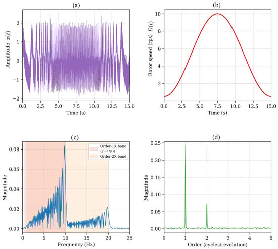
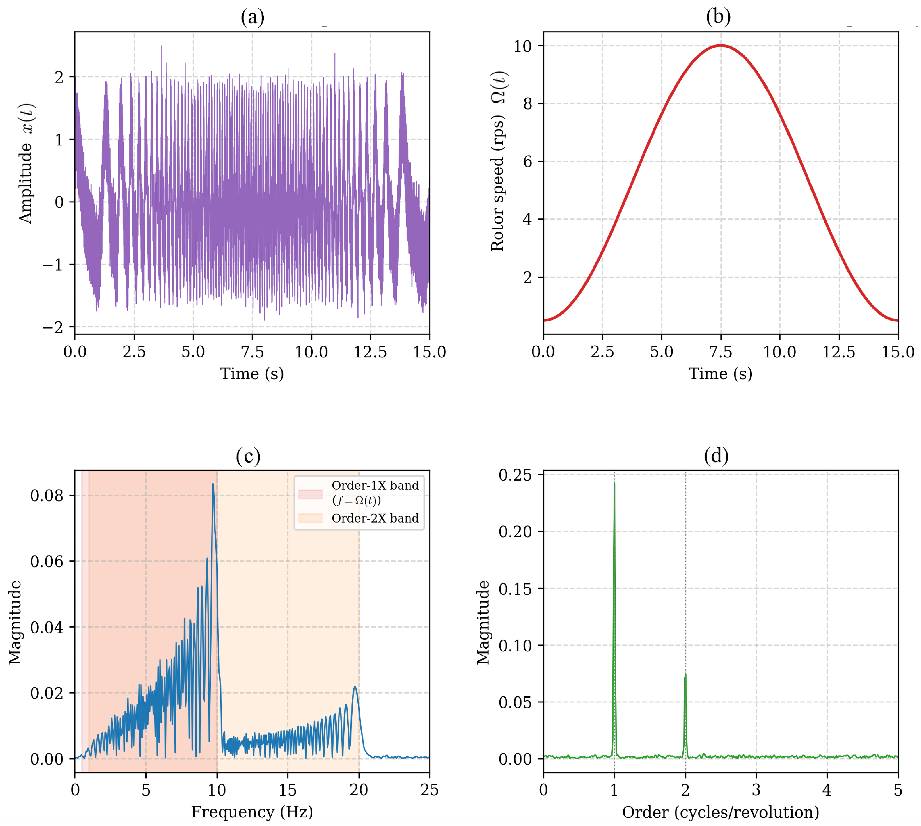
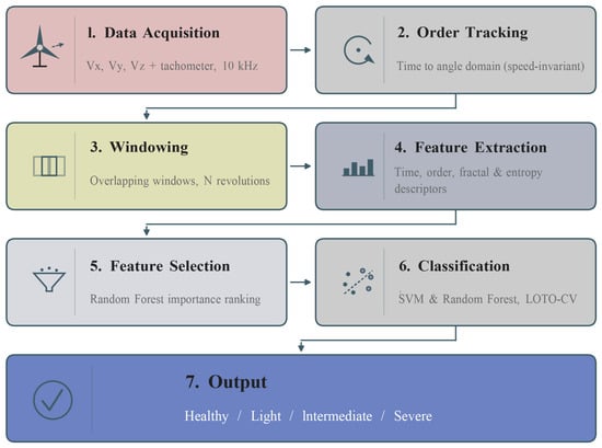
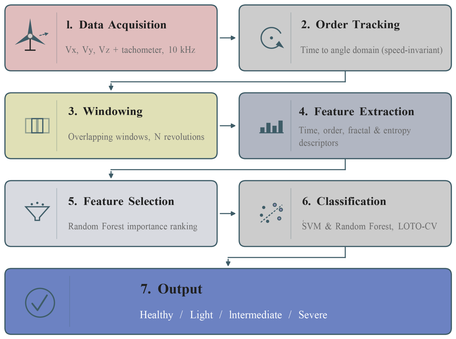
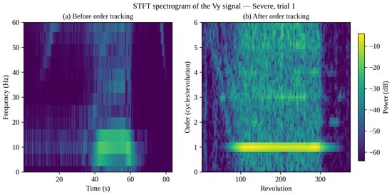
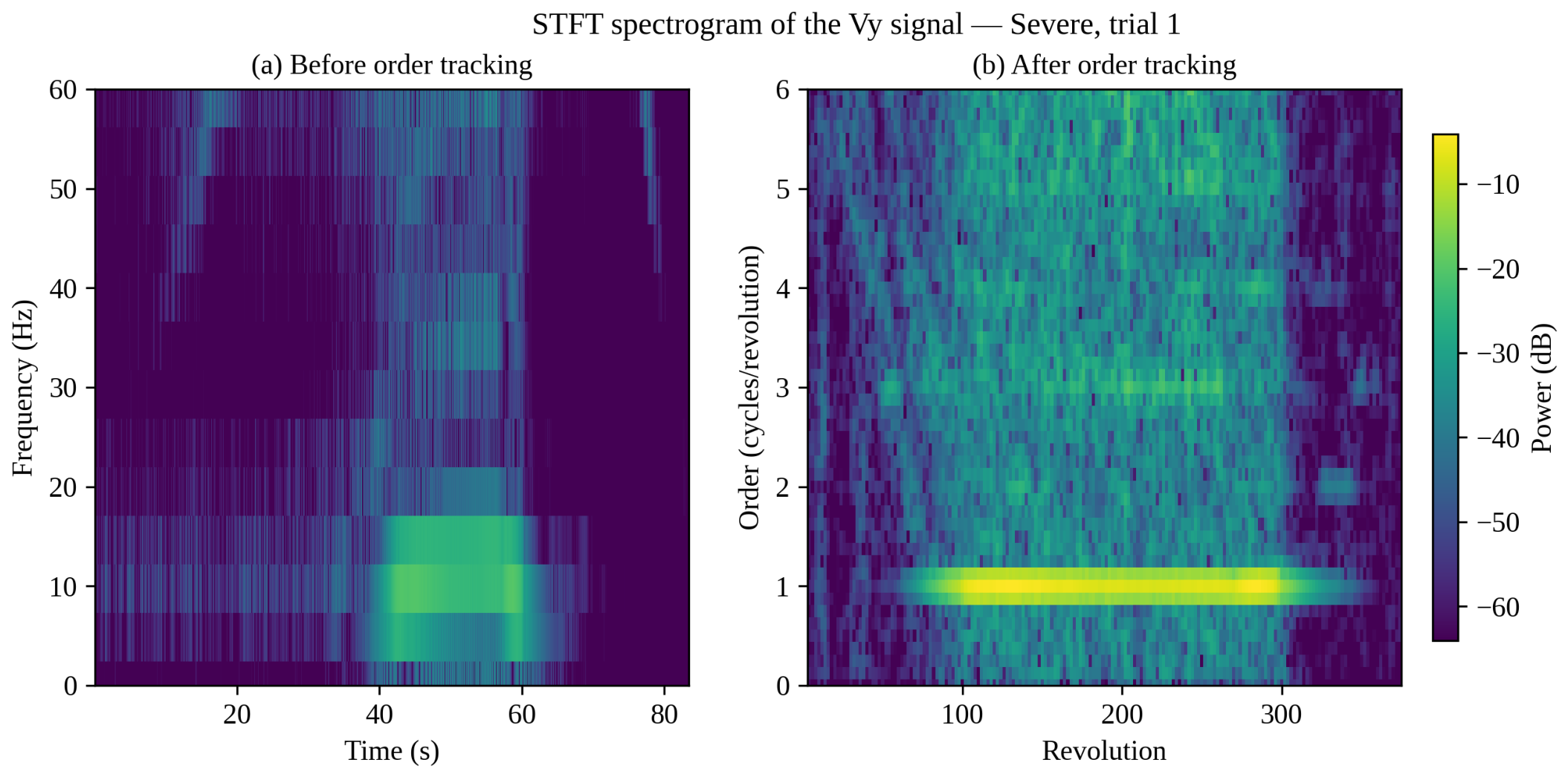
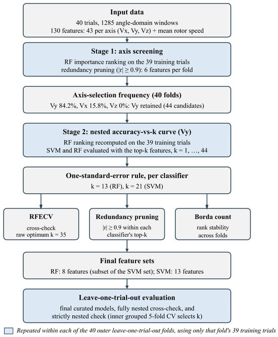
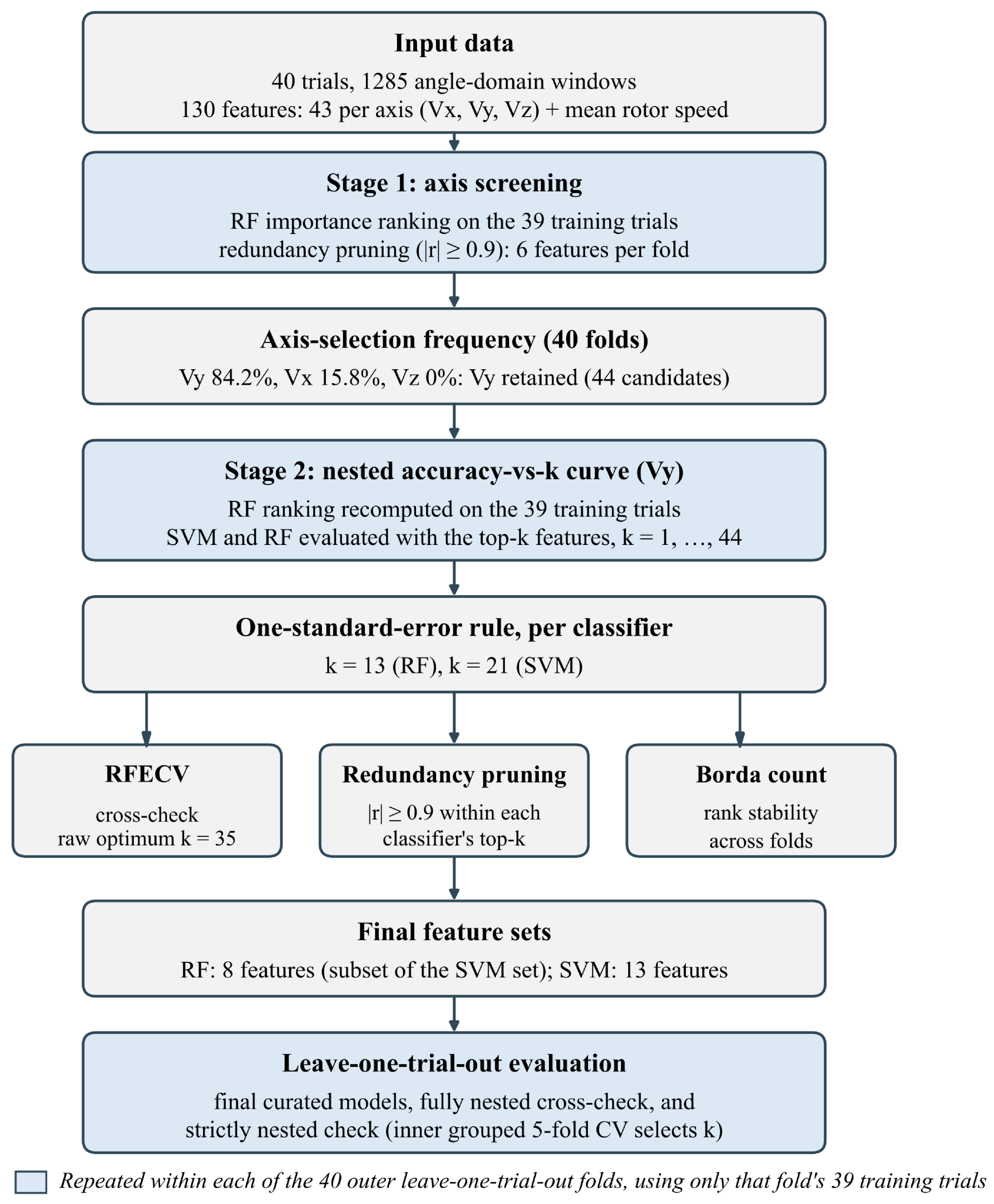
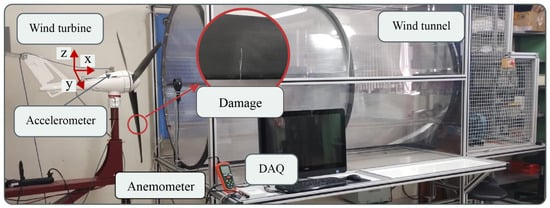
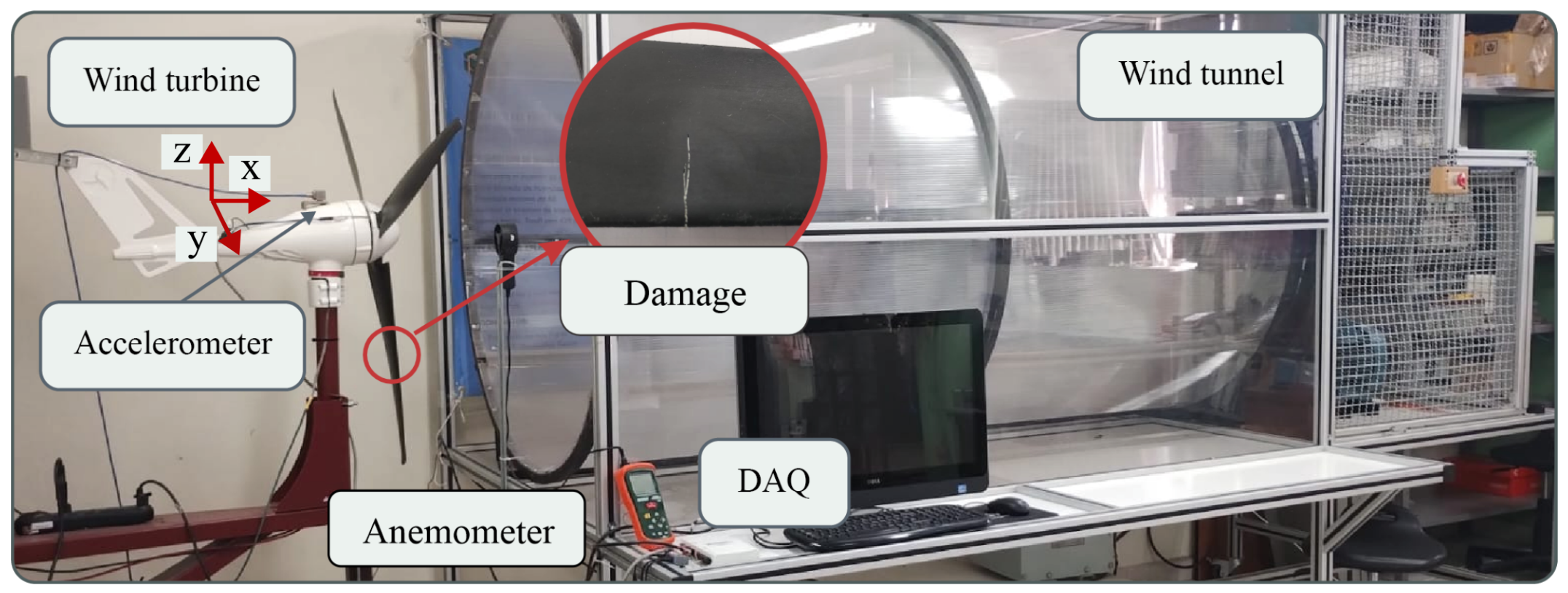
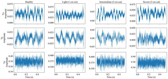
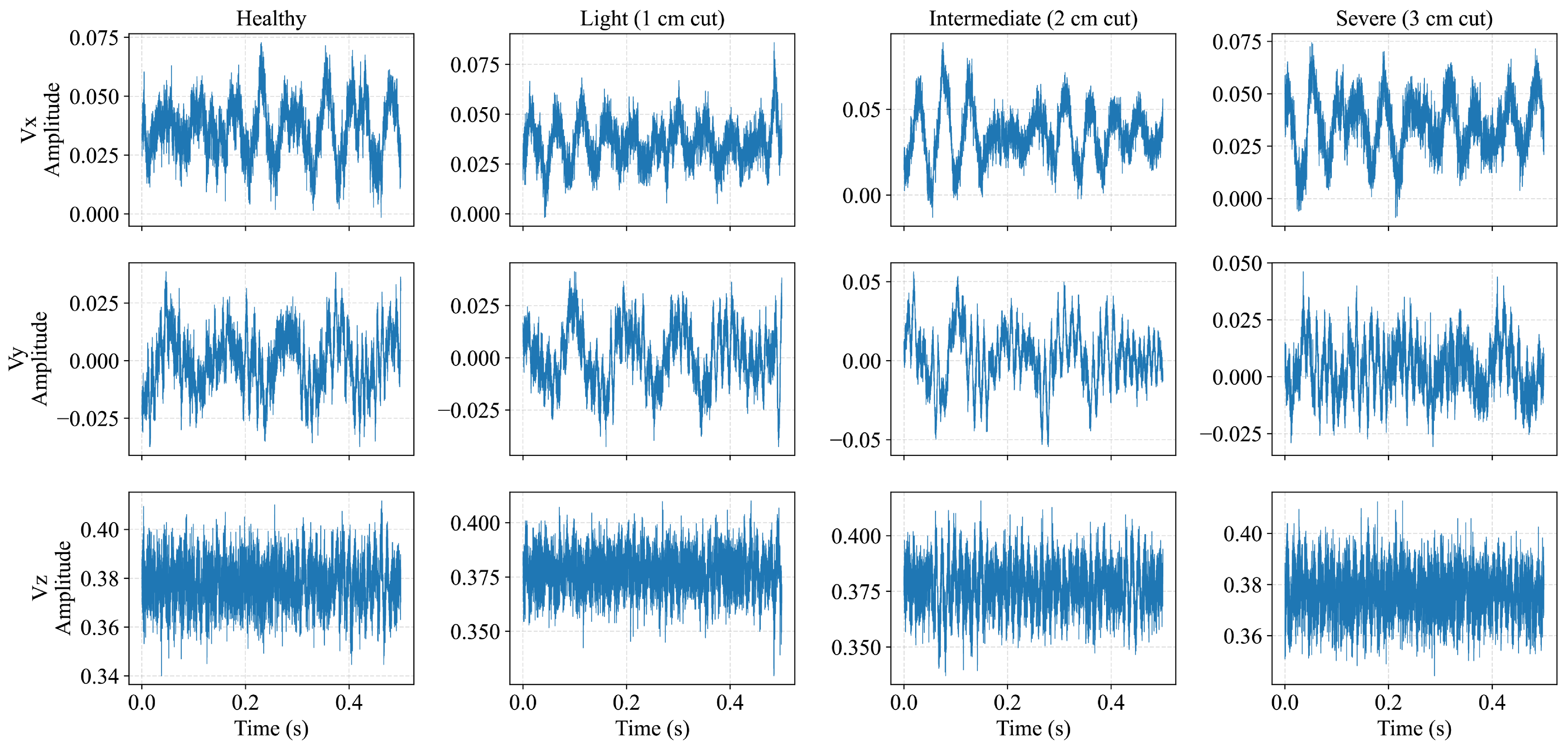
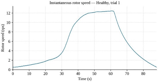
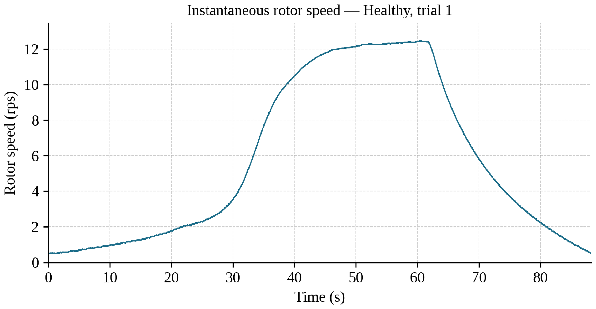
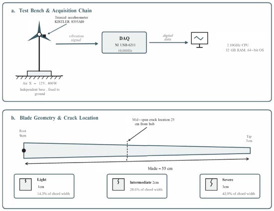
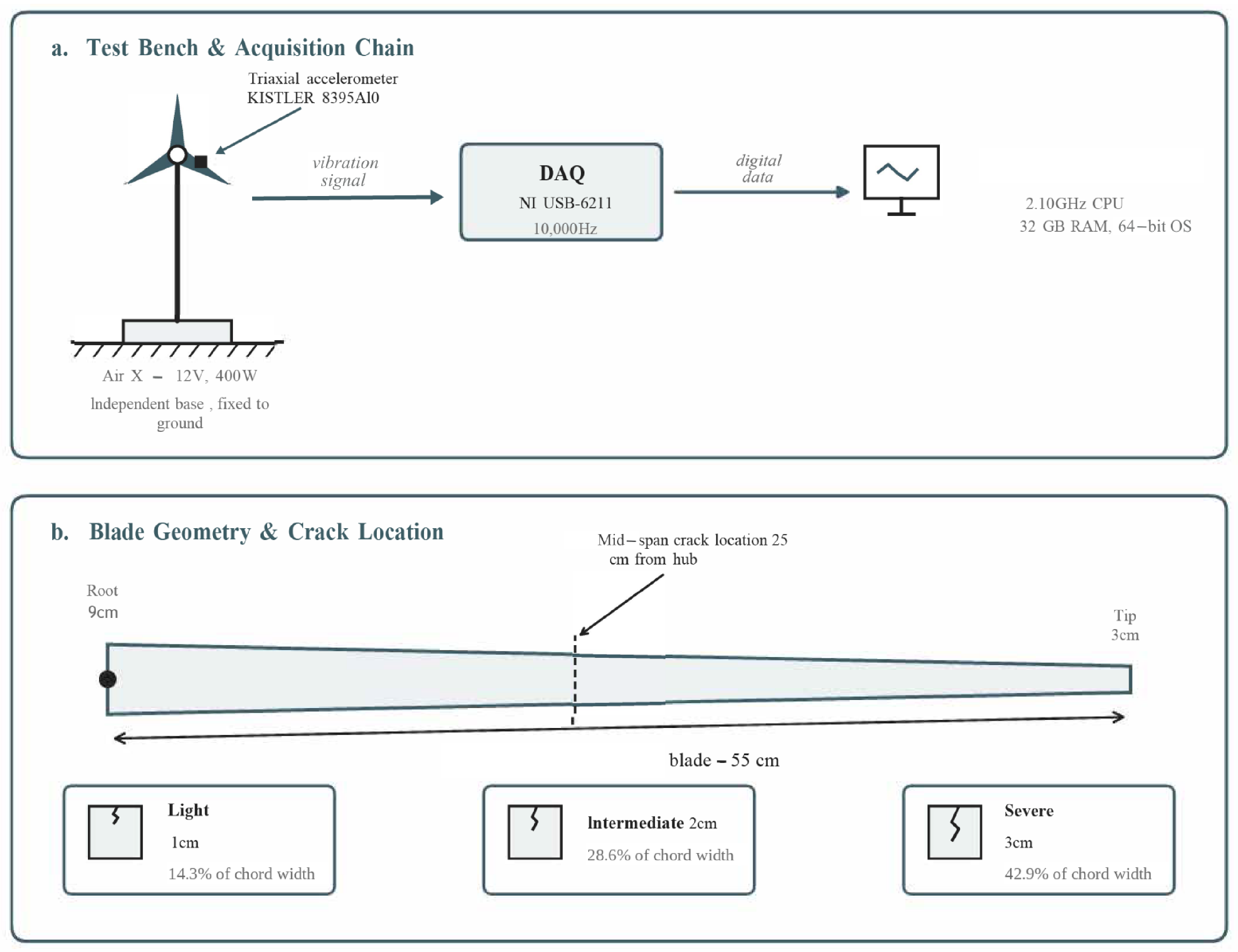
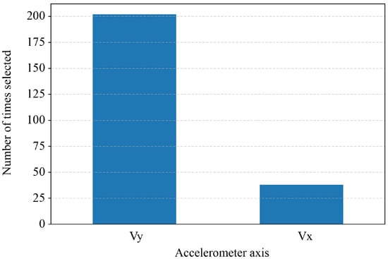
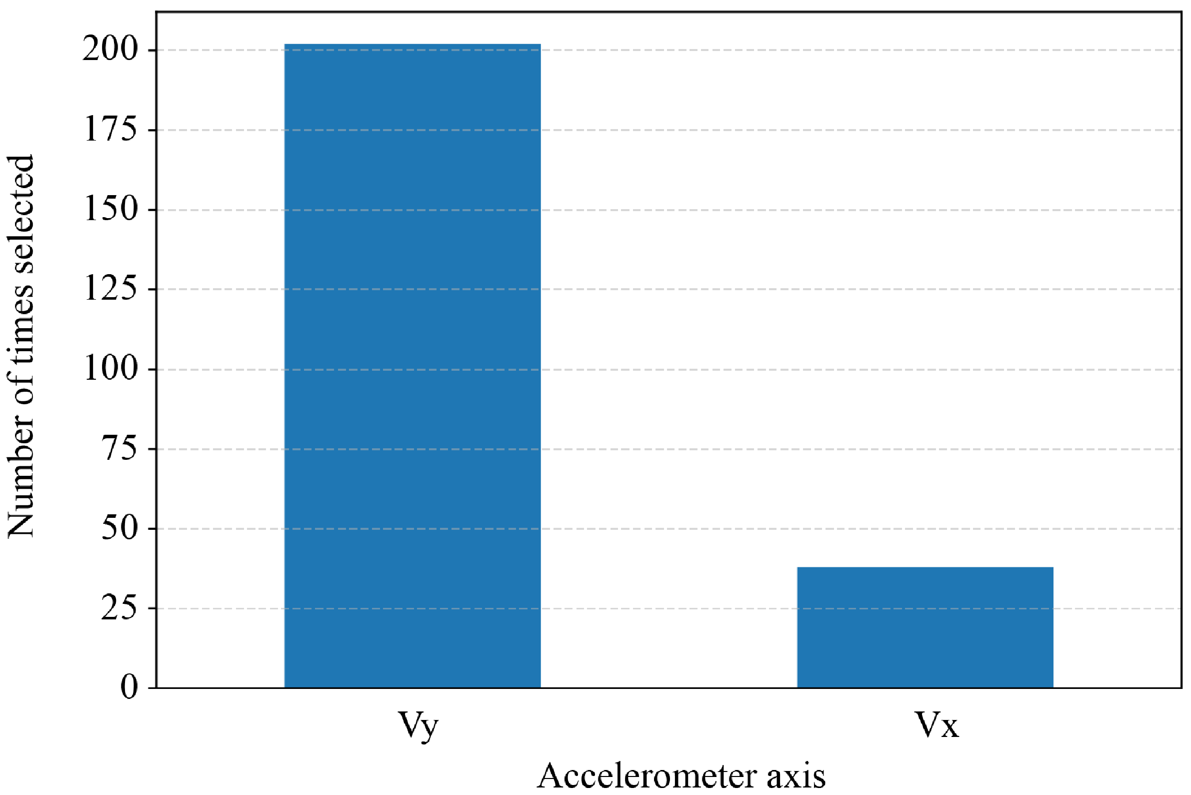
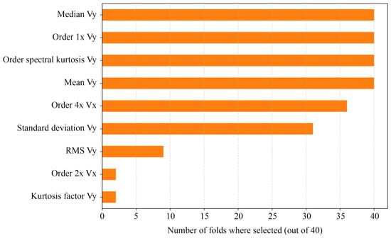
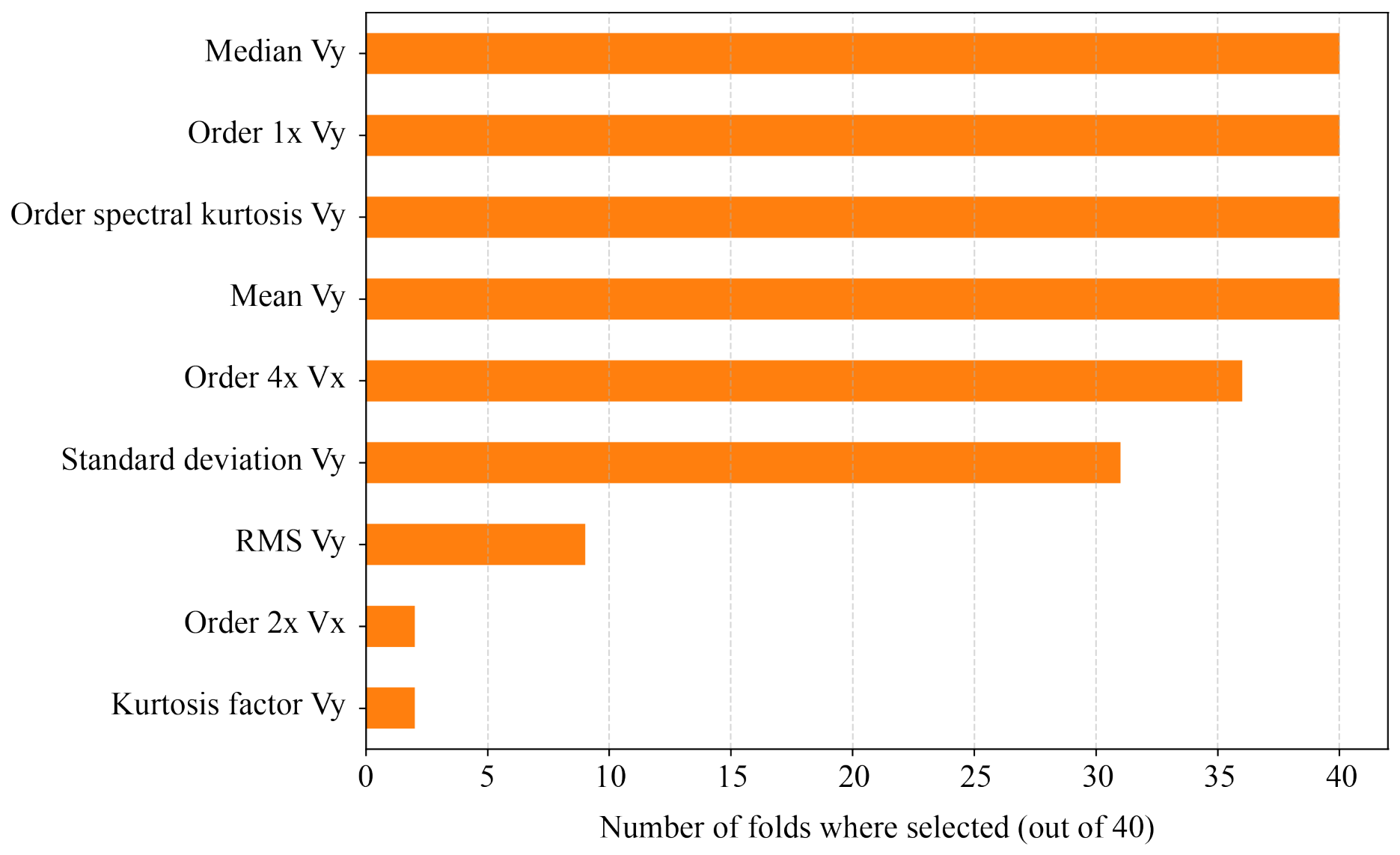
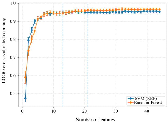
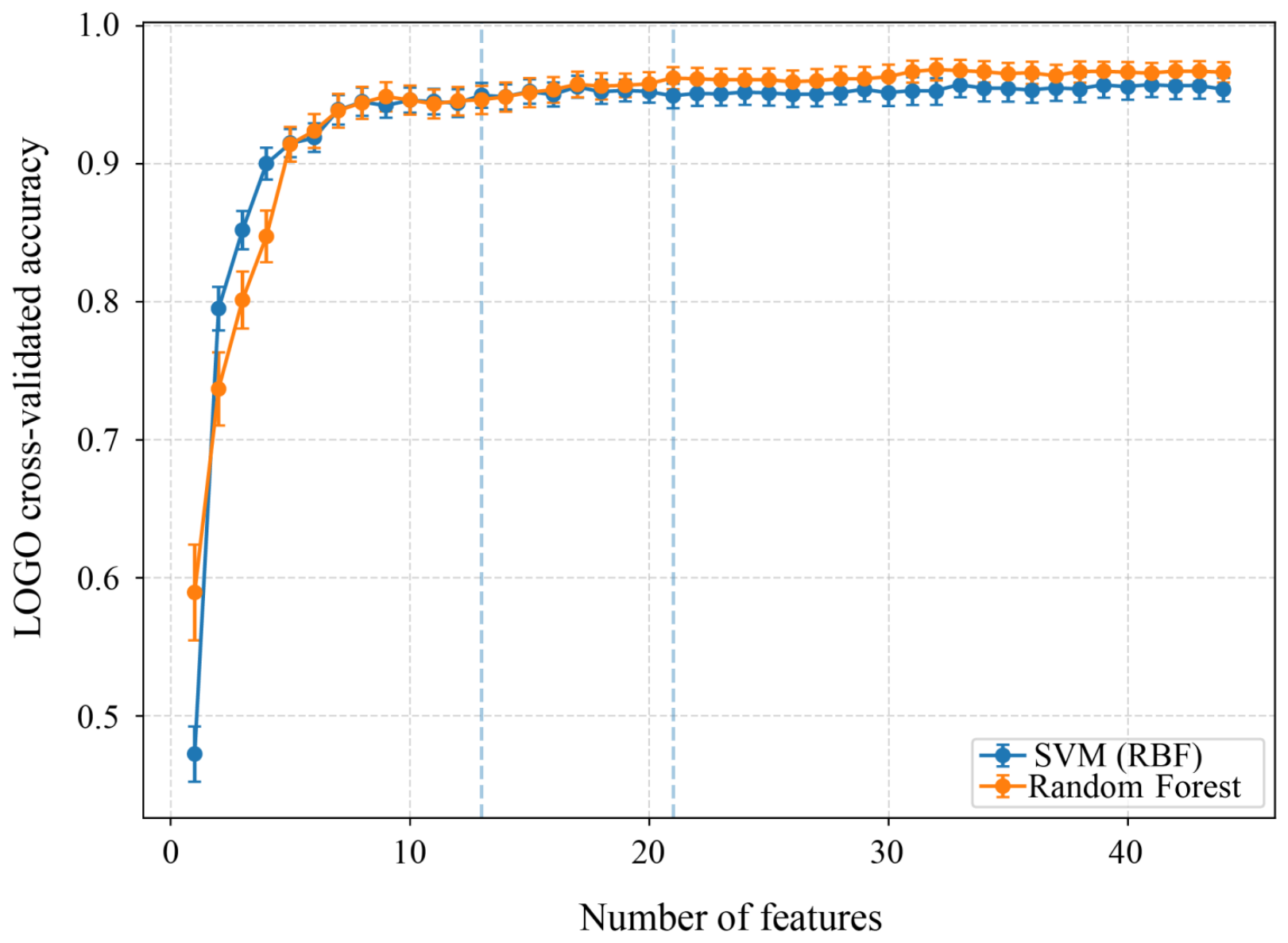
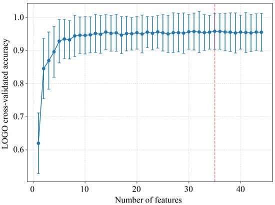
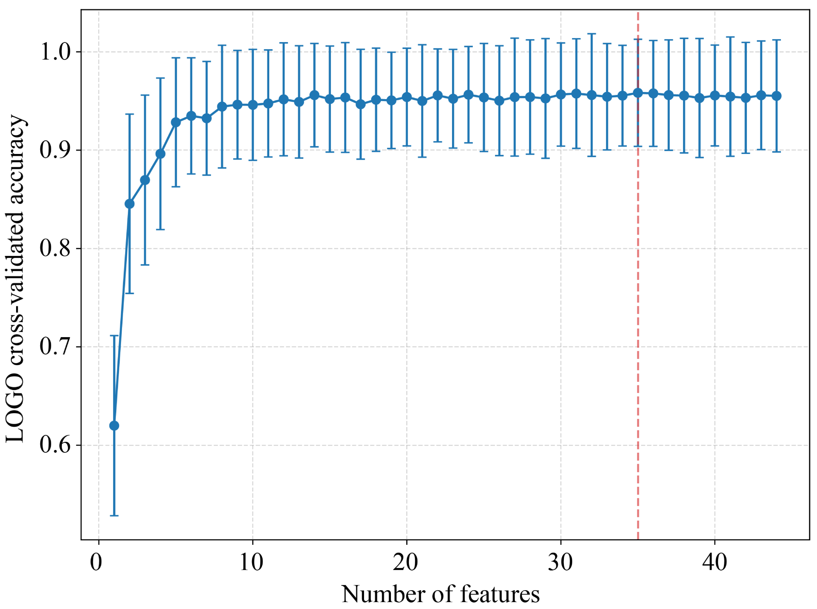
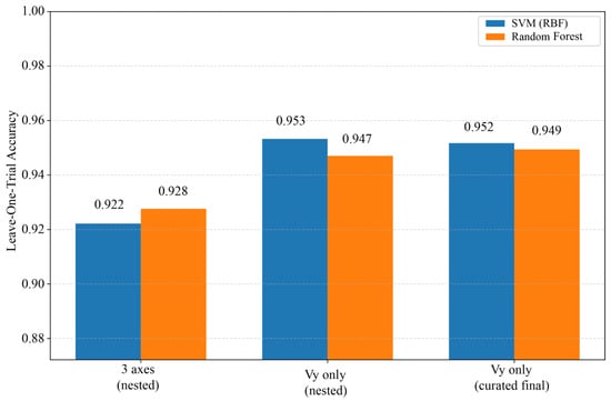
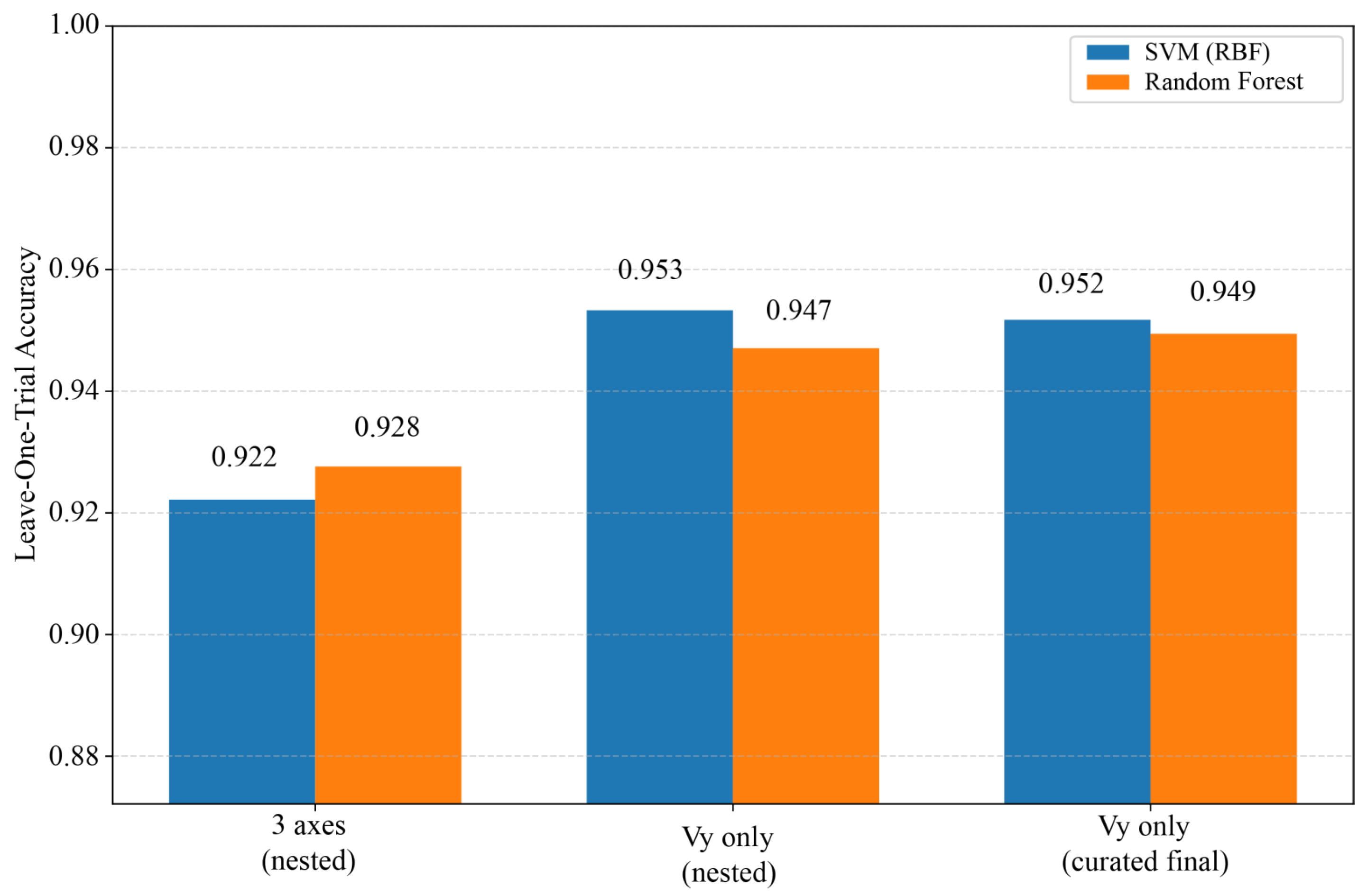
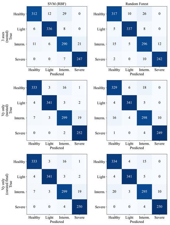
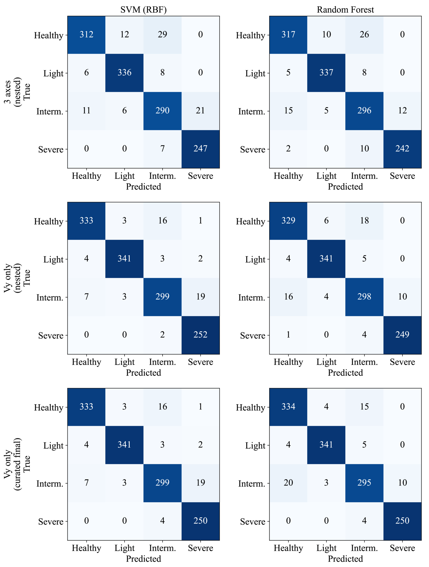
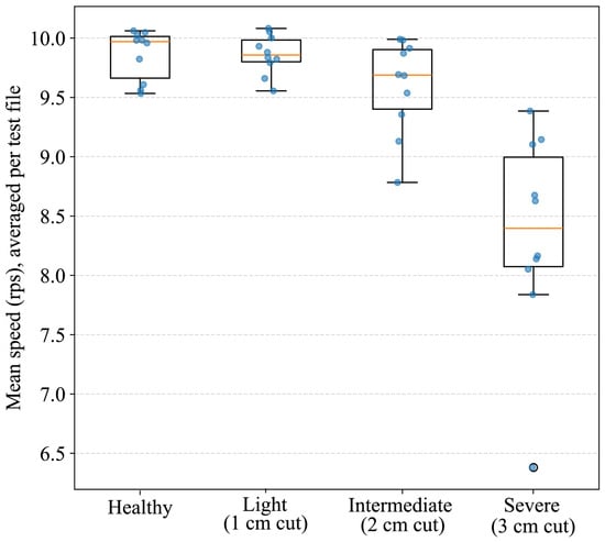
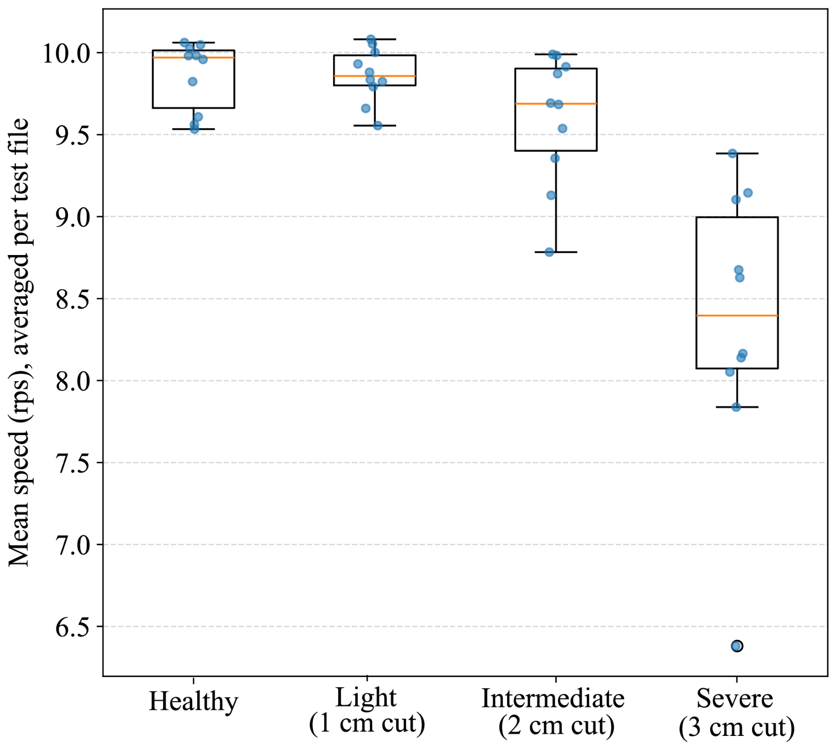

Disclaimer/Publisher’s Note: The statements, opinions and data contained in all publications are solely those of the individual author(s) and contributor(s) and not of MDPI and/or the editor(s). MDPI and/or the editor(s) disclaim responsibility for any injury to people or property resulting from any ideas, methods, instructions or products referred to in the content. |
© 2026 by the authors. Licensee MDPI, Basel, Switzerland. This article is an open access article distributed under the terms and conditions of the Creative Commons Attribution (CC BY) license.