


Highlights
What are the main findings?
- Geographic context classification enables building-level flood vulnerability assessment without site-specific calibration across coastal, fluvial, and pluvial settings, validated across 183 independent locations (AUC 0.855, Spearman ρ 0.746).
- Multi-hazard decomposition separates fluvial, coastal, and pluvial contributions with SHAP attribution identifying dominant drivers, while DEM resolution experiments show global 30 m data produces category reclassification in only 5.3–8.6% of locations.
What are the implications of the main findings?
- The calibration-free design enables pre-construction vulnerability screening at any global location using coordinates alone, shifting flood assessment from post-event damage analysis to prevention-stage planning. Implementation as a web app through Google Earth Engine makes this accessible to non-specialists without GIS software experience.
- Hierarchical integration of heterogeneous data sources (Global Building Atlas + ConvNeXt estimation for building heights; regional 0.5–10 m + global 30 m DEMs) with quantified uncertainty demonstrates a template for global RS applications despite spatially variable data quality.
Abstract
Remote sensing enables building-level flood vulnerability assessment without field surveys, yet existing approaches require site-specific calibration or produce categorical outputs without physical interpretability. We present the Global Flood Vulnerability Model (GFVM), integrating six remotely sensed components (elevation, slope, topographic position index, distance to water, building height, and basement depth) through geographic context classification to quantify vulnerability from terrain and structural characteristics across coastal, fluvial, and pluvial settings. Building heights are extracted primarily from the Global Building Atlas, with gaps filled using a ConvNeXt neural network trained on high-resolution Light Detection and Ranging (LiDAR) ground truth from four cities (within-city MAE 1.35–1.91 m, cross-city MAE 2.05–3.47 m). Terrain metrics are derived from a combination of hierarchical digital elevation models (DEM) (USGS 3DEP 10 m, AHN LiDAR 0.5 m, UK Environment Agency DTM 1 m, Australia 5 m) and global datasets (NASADEM 30 m, Copernicus GLO-30). Hydrographic networks are sourced from OpenStreetMap and Natural Earth. Implementation through Google Earth Engine requires only coordinates as input, returning a five-level vulnerability index with multi-hazard decomposition (fluvial, coastal, pluvial) and SHapley Additive exPlanations (SHAP)-based attribution identifying dominant drivers. Validation across 183 independent locations in Germany, UK, and USA demonstrates robust performance: Area Under Curve 0.855 for separating flooded from non-flooded sites, weighted Cohen’s kappa 0.493 across regulatory zones, and Spearman ρ 0.746 against Federal Emergency Management Agency (FEMA) classifications. Sensitivity analysis across 625 parameter configurations confirms stability, and DEM resolution experiments show that global 30 m elevation data produces category reclassification in only 5.3–8.6% of locations compared to high-resolution sources. Application to the 2024 Kazakhstan floods identifies 118 high-vulnerability locations across 581 assessment points, with vulnerability patterns matching documented inundation. GFVM advances remote sensing applications for disaster risk assessment by demonstrating that multi-source geospatial data fusion enables building-level vulnerability screening without local calibration or field surveys.
1. Introduction
Floods cause widespread structural and economic losses worldwide and remain the most frequent natural disaster, affecting 1.65 billion people, causing 104,614 deaths, and generating more than $651 billion in economic damages between 2000 and 2019 [1,2]. Residential buildings are disproportionately affected not because they are inherently more vulnerable, but because they outnumber other structure types and remain fixed during inundation [3].
Despite these well documented impacts, global investment continues to favor post disaster response over prevention: from 2005 to 2017, 96% of disaster-related spending supported emergency response, reconstruction, and relief, while only 4% was directed toward mitigation and preparedness [4]. Yet evidence shows that proactive risk reduction pays off, for example United States federal mitigation grants save $6 for every $1 spent, and interventions such as acquiring or demolishing flood prone buildings yield $7 in benefits per $1 invested [5].
Flood risk assessment is typically structured around two components: hazard characterization and vulnerability assessment [6,7]. Hazard characterization refers to estimating the probability, spatial extent and intensity of flood events, commonly achieved through hydrodynamic modeling, inundation mapping, and flood frequency analysis [8,9]. Vulnerability describes the susceptibility of exposed elements to damage, shaped by their physical attributes, location, and exposure conditions [10]. Vulnerability, as used throughout this study, refers to the physical susceptibility of a building to flood damage given its locational attributes (terrain position and proximity to water) and structural characteristics such as height and basement depth.
Index-based vulnerability assessments are widely used at regional scales but face challenges in transferability. Studies in Australia’s Hawkesbury–Nepean Catchment [11], Ethiopia’s Amhara region [12], Kashmir [13], and Bangladesh’s Chattogram district [14] show that integrating terrain metrics (elevation, slope, drainage density), land use, and soil properties enables effective local vulnerability mapping. These methods perform well when validated against known flood patterns within their calibration areas. However, they are highly localized, limiting applicability beyond study areas [12,15]; static models cannot reflect changing exposure conditions [12,13]; and validation often relies on single historical events [14] or is entirely absent [13,16].
Beyond these limitations, practical barriers such as technical complexity, data requirements, and lack of accessible implementation platforms also limit adoption by practitioners and non-experts in resource-constrained settings. Comprehensive reviews [17] highlight that indicator-based assessments frequently fail to explain parameter selection or the physical mechanisms justifying component weights. Additional challenges include equal weighting of all terrain indicators, or reliance on expert judgment without sensitivity analysis [13,14] or omission of confidence intervals for vulnerability scores as noted by de Brito and Evers [18]. Most critically, existing indices combine susceptibility into single scores without distinguishing fluvial, coastal, and pluvial mechanisms [19,20,21], obscuring the pathways that determine adaptation requirements.
Recent cloud-based implementations using Google Earth Engine (GEE) demonstrate potential for scalable vulnerability assessment [16,22,23], though these remain regional in scope and rely on machine learning methods that require large labeled datasets and generalize poorly across regions with different hydrological processes. Extracting building heights globally remains challenging due to limited Light Detection and Ranging (LiDAR) coverage and gaps in global building databases, while multi-source DEM fusion requires quantifying uncertainty when integrating regional high-resolution data with global datasets. No existing framework integrates global remote sensing capabilities into a calibration-free flood vulnerability assessment that distinguishes flood mechanisms, explains physical drivers at each location, and remains practical, and usable by non-expert practitioners.
To address these gaps, the Global Flood Vulnerability Model (GFVM) was developed as a globally applicable framework for estimating building-level physical flood vulnerability from remote sensing data without site-specific calibration. GFVM advances remote sensing-based vulnerability assessment through three contributions. First, geographic context classification enables calibration-free vulnerability assessment by integrating six remotely sensed components (elevation, slope, topographic position index (TPI), distance to water, building height, and basement depth) with adaptive weights according to dominant flood mechanisms. Five geographic contexts (coastal, low inland, river valley, mountain, high plateau) adjust component weights to reflect whether vulnerability is controlled by coastal surge, fluvial (riverine) overflow, or pluvial surface-water flooding, eliminating site-specific calibration while maintaining physical interpretability. Multi-hazard decomposition separates fluvial, coastal, and pluvial contributions, with SHAP (SHapley Additive exPlanations) analysis identifying the primary driver at each location.
Second, hierarchical data integration combines the Global Building Atlas with ConvNeXt neural network trained on LiDAR ground truth for building heights, and fuses regional DEM sources (0.5–10 m) with global datasets (30 m). Uncertainty intervals quantify error propagation across heterogeneous terrain and building data sources.
Third, GEE implementation requires only coordinates as input, returning a five-level vulnerability index with mechanism-specific contributions. This enables pre-construction vulnerability screening for building permits and development planning without specialized software, field surveys, or historical damage data, allowing vulnerability assessment to be integrated into planning decisions rather than only post-event response.
GFVM is validated against three independent datasets: observed flood footprints from the Dartmouth Flood Observatory for events in Germany [24], the UK Environment Agency Flood Map for Planning covering three regulatory flood zone categories [25], and Federal Emergency Management Agency [26] multi-hazard designations across riverine, coastal, and pluvial settings. Sensitivity analysis across 625 configurations of relative importance factors for four terrain components (TPI, proximity, slope, and height) tests whether the baseline configuration represents a robust solution or fragile one. Ablation experiments across four contrasting terrain types (Netherlands coastal flat, Thames Valley, Sydney Basin, Florida lowland) quantify each component’s contribution to the final index. Digital elevation model (DEM) resolution comparison between high-resolution sources (0.5–10 m) and global NASADEM (30 m) assesses whether terrain generalization introduces systematic bias in vulnerability estimation.
Application to the 2024 Petropavlovsk flood (Kazakhstan) demonstrates operational utility. The model assesses 581 locations across five neighborhoods and attributes vulnerability to fluvial versus pluvial mechanisms. When paired with flood frequency and depth data, the vulnerability index supports full risk quantification; without hazard information, it still guides land use decisions and retrofit priorities.
2. Methods
The GFVM methodology follows the two-stage workflow described in Section 2.3. Section 2.1 and Section 2.2 describe the data sources and building height extraction methods. Section 2.3 describes the GFVM architecture: geographic context classification in Stage 1, component scoring and weighted aggregation in Stage 2, and multi-hazard decomposition. Section 2.4 describes the model’s web interface. Section 2.5, Section 2.6 and Section 2.7 describe four analyses characterizing model behavior: weight sensitivity, component contribution, and DEM resolution effects. Section 2.8 describes operational evaluation.
2.1. Data Sources
GFVM uses globally available remote sensing datasets to enable vulnerability assessment at the global level. Terrain metrics (elevation, TPI, slope) come from digital elevation models through hierarchical source selection that prioritizes the highest resolution available (Table 1). Regional sources include USGS 3DEP (10 m, USA), AHN2 and AHN3 (0.5 m LiDAR, The Netherlands), UK Environment Agency DTM (1 m), and Australia 5 m DEM. Global coverage defaults to NASADEM (30 m), Copernicus GLO-30 (30 m), and ALOS World 3D (30 m). This hierarchy balances local accuracy with global applicability, and operates through a simple rule: the model uses the highest-resolution DEM available for a given location, falling back to global 30 m sources where high-resolution regional datasets are absent. This integrated strategy ensures global coverage while maintaining internal consistency in terrain-derived components.
Water proximity is derived from OpenStreetMap’s (OSM) hydrographic network (rivers, streams, lakes, coastlines) via the Overpass API, with Natural Earth providing fallback where OSM mapping is sparse. Significant water bodies are filtered from ornamental features using geometric criteria (minimum 500 m2 area, >10 geometry nodes) and tag-based classification to exclude fountains or decorative ponds.
Building height is extracted primarily from Global Building Atlas (GBA) [27], which provides near-global coverage of building height information. In locations where GBA height is unavailable, building height is estimated using a convolutional neural network trained on high resolution reference datasets from four cities: Vienna (200,000+ footprints, 0.5 m DSM and 1 m DTM) [28], Paris (198,000 footprints, 0.5 m LiDAR HD) [29], Astana and Barcelona (11,000 and 16,500 cadastral footprints from Maxar Technologies, Westminster, CO, USA). Overhead RGB satellite imagery was retrieved at zoom level 20 (0.07–0.15 m ground sampling distance), producing 425,000 training instances.
Table 1.
Summary of the datasets used for model development, validation, and application.
Model evaluation used three independent datasets covering observed flood events, regulatory classifications, and multi hazard zones. Event observations in Germany were taken from the Dartmouth Flood Observatory and included 51 points, with 32 mapped as flooded and 19 mapped as non-flooded. Regulatory comparison in the United Kingdom used 59 locations drawn from the UK Environment Agency Flood Zone system, covering 16 Zone 1 sites, 22 Zone 2 sites, and 21 Zone 3 sites. A third dataset covered FEMA flood designations at 73 sites spanning riverine, coastal, pluvial, and mixed hazard settings. FEMA categories were grouped into a four-level ordinal scale: low (X unshaded), moderate (X shaded), high (A, AE, AH, AO), and very high (VE). This set contained 12 low vulnerability, 9 moderate vulnerability, 33 high vulnerability, and 19 very high-vulnerability samples.
2.2. Building Height Extraction
Building height was obtained primarily from the GBA by querying footprint-level height attributes within a local spatial buffer around each target location. To ensure height estimates in regions without GBA coverage and to enable internal consistency checks, a supervised height estimation model was trained using high-resolution reference data described in Section 2.1. Reference building heights were derived by subtracting DTM from DSM for each footprint. For Vienna, DSM was resampled from 0.5 m to 1 m to match DTM resolution. Heights below 2 m were excluded as likely measurement artifacts. Extraction accuracy was assessed against official government reference dataset from Paris and Vienna [30,31] using mean absolute error (MAE), root mean square error (RMSE), and coefficient of determination (R2). A supplementary point-level-validation against Google Earth height measurements for 20 randomly selected buildings across Vienna and Paris provides an additional assessment of real-world estimation accuracy.
For model training, overhead RGB image tiles were centered on each building, cropped, resized to 224 × 224 pixels, and normalized using ImageNet statistics. To prevent spatial leakage, a grid-based spatial split was applied within each city, assigning entire grid cells to training, validation, and test sets in a 70/15/15% ratio (Figure 1). To address the long-tailed height distribution, data augmentation combined standard stochastic transformations with targeted oversampling of buildings. The height prediction model employs ConvNeXt [32] as the visual backbone, initialized with ImageNet-pretrained weights [33] and trained using the AdamW optimizer [34] with a cosine-annealing learning-rate schedule.
Figure 1.
Spatial train, validation, and test splits for (a) Astana, (b) Barcelona, (c) Paris, and (d) Vienna using grid-based partitioning. Blue grids were used for train, green for validation, and orange for testing.
2.3. Flood Model Architecture
GFVM runs on two-stage architecture (Figure 2). In Stage 1, geographic context is classified using rule-based thresholds of elevation, TPI, and distance to surface water (Table 2). These criteria allow the classification of five distinct settings: Coastal zones, defined as areas below about 10 m [35,36] and close to the shoreline, where surge and tidal effects are amplified. River valleys (100–300 m, negative TPI, near rivers) typically represent channel-adjacent terrain with overbank flooding as the primary inundation mechanism, consistent with flood-susceptibility studies showing that low-elevation areas close to rivers are the most flood-prone zones [37,38]. Low inland areas (10–100 m) tend to accumulate water due to gentle slopes and poor drainage, whereas mountainous terrain (300–600 m) and high plateaus (>600 m) generally reduce flood propagation through reduced catchment connectivity and gravity-driven drainage, except where local depressions occur.
Figure 2.
Global flood vulnerability model (GFVM) architecture overview. Vertical arrows represent hierarchical DEM selection; horizontal arrows represent component-level outputs.
Table 2.
Component weights and physical basis used in the flood vulnerability index.
Each context applies an adjustment factor that influences the final vulnerability score to reflect the dominant flood mechanisms. This terrain-based classification provides contextual information only; the fluvial, coastal, and pluvial components themselves are defined and computed entirely in Stage 2 which scores six components: Proximity, slope, TPI, elevation, building height and basement depth, then aggregates them through weighted combination to produce the final vulnerability score.
Equations (1)–(6) shows how each component is transformed into a normalized vulnerability score (0–1) through piecewise functions calibrated to flood dynamics. TPI is the dominant factor in GFVM, with its relative importance estimated at approximately 35%. TPI reflects local elevation context rather than absolute elevation, enabling identification of depressions and valley bottoms, areas consistently recognized as primary flood initiation zones [39,40].
Negative TPI values indicate topographic depressions where surface water accumulates. The −5 m threshold separates shallow swales from pronounced valleys that concentrate drainage from upslope contributing areas. Positive TPI (ridges and hilltops) reduces vulnerability through gravity-driven drainage away from the assessment point.
Proximity to water accounts for 30% of the vulnerability score, reflecting its established role in controlling overbank flooding during moderate to extreme events because buildings near rivers or coasts face higher exposure [42], with machine learning studies identifying distance to streams as a key factor, with relative importance of 0.43 on a 0–1 scale [41].
where is the elevation adjustment factor and is distance to the nearest significant water body.
where is elevation above sea level.
The 100 m threshold corresponds to standard practice in flood vulnerability indices, where it captures very high exposure to flooding across diverse sources, while the gradual decay to 5 km outer bound captures residual risk from extreme events [46,47]. The elevation adjustment factor reduces proximity scores above 500 m because high-elevation rivers and lakes generate limited inundation [48,49].
The influence of slope on flood susceptibility varies considerably across regions. Tetteh et al. [43] found slope accounted for 16.6% of flood susceptibility in multivariate models, Kasahun et al. [37] reported 26.3% in South Ethiopia and Burayu et al. [50] found 32% to be sufficient in Oromia. Based on these findings, we adopted a global weight of 20% for slope. Flat or gently sloping areas impede drainage, while steeper gradients promote runoff [40]. GFVM reflects these dynamics by converting the raw slope values into piecewise function and assigning higher vulnerability weight to low-slope terrain and lower scores to steeper ground, consistent with hydrological principles and recent studies [38,51].
where s is the slope.
The minimum score of 0.5 reflects residual vulnerability from concentrated flow paths even on steep terrain.
Elevation is not assigned a direct weight because it operates as a structural control that shapes geographic context, modifies proximity through the elevation adjustment factor, and forms the base surface from which slope and TPI are derived. Its influence is therefore expressed through those components rather than as a separate weighted term. Structural vulnerability is represented through building height (15%), which captures vertical clearance from flood stages and the exposure of floor-levels. Prior studies show that structural attributes influence vulnerability but do not override terrain-driven controls in urban vulnerability assessments [44,45].
Basements introduce additional vulnerability through below-grade exposure to groundwater intrusion and limited egress during rapid-onset flooding. When basements are present, component weights shift: building height increases to 30% (from 15%), TPI drops to 30% (from 35%), proximity reduces to 25%, and slope to 15%. Basement depth is an optional user-supplied input; when it is not provided, the model defaults to zero basement depth and applies the standard above-grade component weights. A depth-dependent multiplier increases vulnerability by 15% per meter of basement depth, reflecting the additional failure pathways of subsurface spaces such as hydrostatic pressure on foundation walls, groundwater intrusion through floor slabs, and restricted egress that are absent from above grade structures. This assumption is supported by the sensitivity analysis in Section 2.5, which shows that building height parameters do not govern ordinal rankings at the composite vulnerability index level.
where H is the elevation of the building.
The ground-level structures () offer no vertical buffer against inundation. The non-zero floor (0.1) acknowledges that even elevated structures face infrastructure damage from extreme events.
These weights represent informed initial estimates, defined prior to validation and not adjusted to improve performance on any validation dataset. To evaluate robustness, we conducted a sensitivity analysis across different weight combinations spanning ±20% perturbations of baseline values (see Section 2.5 for details).
The final vulnerability index is given as:
where: are component scores (i.e., 30, 35, 20, 15) for proximity, TPI, slope and building height respectively.
The base model extends to multi-hazard assessment by decomposing vulnerability into three flood mechanisms: fluvial, coastal, and pluvial (Equations (7)–(13)). Fluvial vulnerability captures riverine flood exposure through water proximity, topographic position relative to channels, and drainage characteristics
In our approach, coastal vulnerability peaks below 2 m within 5 km of the shoreline, declines with elevation to a residual level by 10 m, and then decreases with distance from 5 km to 20 km, with lower elevations retaining higher residual vulnerability.
where is distance to coastline.
For pluvial vulnerability, we combine normalized TPI and slope to identify poorly drained areas, with TPI weighted slightly higher than slope. We also applied an elevation decay function ) that reduces vulnerability scores above 200 m and decreases linearly to 0.1 above 1000 m to account for lower precipitation intensity and higher infiltration capacity at altitude.
where and are normalized factors derived from the TPI and slope scoring functions (Equations (10) and (11))
The three hazard components are combined using adaptive weights (Equation (13)) that reflect dominant flood mechanisms for each elevation context. These weights mirror the typical influence of surge (coastal), river overflow (fluvial), or surface-runoff (pluvial) processes across terrain settings, ensuring that the vulnerability index assigns greater influence to the mechanisms most responsible for driving exposure and damage in each class. Coastal zones assign weights of 0.50 to coastal processes, 0.30 to fluvial, and 0.20 to pluvial, emphasizing surge-related risk. Low inland areas balance riverine and surface water threats, weighting fluvial and pluvial processes at 0.50 and 0.40 respectively with minimal coastal contribution. Elevated regions assign zero coastal weights, distributing influence between fluvial and pluvial processes at 0.60 and 0.40 respectively. Complete scoring functions and implementation details are available in the Github repository (https://github.com/Gunjuzone/flood-vulnerability-api, accessed on 19 January 2026).
where , and are context-dependent adaptive weights for fluvial, coastal, and pluvial hazard components respectively.
Additionally, we incorporate SHAP decomposition to support transparency and vulnerability communication. A Random Forest surrogate model (R2 > 0.95) trained on 1000 globally distributed locations is used to decompose vulnerability indices into component-level contributions. SHAP thereby translates the composite index into physically interpretable terms: a location where proximity is the primary contributor indicates that water exposure is the controlling condition and interventions such as riparian setbacks or protective barriers may be most effective, whereas a location dominated by TPI reflects a topographic depression where drainage improvements would be more impactful. This interpretability layer provides a clear link between the composite index and the physical factors driving site level susceptibility.
2.4. GFVM Interface
The flood-vulnerability application runs on a FastAPI backend powered by GEE. The interface is accessible through web browsers on desktop or mobile devices at: https://huggingface.co/spaces/GeoOrg13/flood-vulnerability. The landing page provides four entry options: (1) Basic Assessment, (2) Detailed Explanation, (3) Multi-Hazard Analysis, and (4) Batch Upload (Figure 3). Users enter latitude and longitude (WGS84) manually for point-based assessment and may optionally specify building height and basement depth or predict building height using the predict option.
Figure 3.
(a–f) Illustrates the user interface flow of the GFVM web application, showing how users navigate from data entry to vulnerability outputs and multi-hazard summaries.
For each query, the backend retrieves elevation, slope, and TPI from the global DEM via GEE and extracts water-network proximity using OpenStreetMap hydrological features. Basic assessment returns the vulnerability index, assessment confidence, and terrain analysis. Detailed Explanation provides the same information plus detailed vulnerability factor analysis. Multi-Hazard Analysis offers the same data but replaces vulnerability factor analysis with a breakdown of hazards (fluvial, coastal, and pluvial pathway scores) and the dominant hazard. Batch Upload accepts CSV files in place of single-point entry and can perform basic or multi-hazard evaluations. Single-point results appear on the web interface and the Batch assessment results export automatically in CSV.
2.5. Weight Sensitivity Analysis
The sensitivity analysis evaluates whether the fixed component weights in Equation (6) influence the stability and robustness of the model’s predictions across independent validation datasets. Weight sensitivity was assessed using a full-factorial design in which the weights assigned to the four terrain components (proximity, TPI, slope, and height) were systematically varied across five levels (−20%, −10%, baseline, +10%, +20%), producing 625 weight configurations (54). For each combination, terrain metrics were precomputed to avoid repeated API calls, and GFVM was run against the three validation datasets (FEMA flood categories, UK flood zones, and Germany event observations). Only latitude and longitude coordinates were used, with height and basement set to zero for all samples, ensuring that any observed sensitivity originated solely from terrain features rather than building characteristics. Performance was assessed using Kendall’s τ and Spearman’s ρ to evaluate ordinal agreement, and MAE to quantify deviations in vulnerability magnitude.
2.6. Component Contribution Experiment (Ablation Study)
The ablation study evaluated the influence of each GFVM component by measuring the effect of removing individual contributors. Unlike the weight sensitivity analysis, which tests parameter variation, ablation isolates the contribution of the terrain metrics by disabling them one at a time. GFVM ran once with the full configuration, then repeated with specific components disabled. When a component was disabled, its score was replaced with a neutral value of 0.5 and its weight was redistributed among the remaining active components to preserve a valid convex combination.
The analysis was conducted across four regions representing distinct terrain conditions: a flat coastal corridor in the Netherlands, the Thames River valley, an urban coastal setting in Sydney, and a low inland floodplain in Florida. For each region, random points were sampled within predefined geographic bounds, and terrain metrics were extracted for all ablation configurations. Each ablation run produced a vulnerability index, categorical vulnerability class, and internal component scores for each sampled point.
2.7. DEM Resolution Experiment
This experiment validates the hierarchical DEM selection strategy described in Section 2.2 by quantifying how substituting high resolution regional DEMs with the global 30 m NASADEM affects terrain-derived metrics and the resulting vulnerability index. The four regions used in the ablation study (Netherlands, Thames Valley, Florida, and Sydney) were sampled uniformly using random latitude and longitude points within predefined geographic bounds. For each point, elevation, TPI, and slope were computed using the designated high-resolution DEM: AHN2 and AHN3 (0.5 m) for the Netherlands, the Environment Agency 1 m LiDAR grid for the Thames Valley, USGS 3DEP 10 m for Florida, and the national 5 m DEM for Australia. These high-resolution DEMs serve as benchmarks for quantifying resolution effects. The same points were then re-evaluated with NASADEM (30 m), producing matched pairs of terrain metrics and vulnerability outputs for every location.
The outputs included the absolute change in the vulnerability index, the elevation difference between DEMs, the corresponding changes in slope and TPI, and the resulting change in vulnerability category. This provides a direct quantification of how DEM resolution differences propagate through terrain metrics and ultimately affect the vulnerability model.
2.8. Operational Evaluation
The operational evaluation tests whether terrain-driven vulnerability patterns identified by GFVM correspond to documented flood impacts when applied in an independent region. This evaluation was carried out using the 2024 historical flooding in some regions of Kazakhstan. In April 2024, the Ishim River flooded Petropavlovsk in Northern Kazakhstan, displacing over 5000 residents and inundating almost 1000 homes. The event combined several factors: rapid snowmelt, heavy rains, frozen soil preventing infiltration, dams breached, reservoirs overflowed, and rivers burst their banks.
To perform an operational analysis, five neighborhoods representing different topographic settings were selected: Zarechnyi, Teplichnoye, Pribrezhnoy, Podgora, and Khromzavod. Assessment points were systematically selected on a 100 m grid across the five zones, totaling 581 locations. Building height and basement depth were set to zero, isolating terrain-driven vulnerability. Model outputs were compared against qualitative flood impact reports from regional authorities and satellite imagery documenting inundation extent. Performance was assessed through spatial correspondence between high-vulnerability zones and reported flooding concentrations, and through consistency between dominant hazard attribution and observed flood mechanisms. Results are reported in Section 3.6 and interpreted in Section 4.6.
3. Results
3.1. Model and Building Height Performance
The ConvNeXt model achieved MAE of 1.35–1.91 m under within-city hold-out evaluation across four training cities (Table 3). Leave-one-city-out evaluation produced MAE of 2.05–3.47 m, showing expected performance reduction under domain shift. Tall building augmentation reduced MAE in the tallest height bin from ~12 m to ~8.5 m (Figure 4a).
Table 3.
Evaluation results of the ConvNeXt model for within-city and cross-city testing.
Figure 4.
(a) Per-bin MAE across buildings, with sample counts shown on a log scale (b) Independent point validation of the model against google earth buildings.
Ground truth validation against official cadastral datasets from Paris and Vienna showed RMSE between 3.62 and 5.15 m when comparing DEM-derived heights with reference data. The GBA produced MAE of 3.18 m (Vienna) and 5.02 m (Paris) with RMSE of 4.99 m and 6.86 m respectively. As supplementary point-level verification, independent validation against Google Earth height measurements in Vienna and Paris produced overall MAE of 0.94 m and RMSE of 1.34 m (Figure 4b), with one Vienna building showing the largest deviation of 4.27 m against a measured height of 15 m and the remaining nineteen below 2.3 m.
3.2. Sensitivity Analysis
Table 4 summarizes the distribution of performance metrics across component weight permutations (n = 625). Kendall’s τ, Spearman’s ρ, and MAE remains within narrow ranges in all datasets. FEMA shows τ values between 0.671 and 0.730 (mean 0.706), while Germany spans 0.435 to 0.494 (mean 0.462), and the UK spans 0.518 to 0.611. Spearman’s ρ shows a similar pattern with low variation, and MAE values remain tightly clustered within each dataset.
Table 4.
Model sensitivity performance across the tested range for the FEMA, Germany, and UK.
Figure 5 illustrates the effect of varying proximity and TPI weights while keeping slope and height weights fixed at their baseline values (0.20 and 0.15). White diamonds mark the baseline configuration (proximity 0.30, TPI 0.35) on each panel. Performance surfaces are smooth, with gradual changes across weight dimensions, and no abrupt transitions. Contour lines are widely spaced in all cases, though FEMA panels display marginally steeper gradients compared to Germany and the UK, whose surfaces remain relatively flat.
Figure 5.
Sensitivity of performance metrics to proximity and TPI weights (slope and height fixed at baseline 0.20 and 0.15). White diamond mark the baseline configuration (proximity 0.30, TPI 0.35).
The baseline configuration lies close to the corresponding means for all three datasets. For FEMA, the baseline Kendall’s τ is 0.698, marginally below the overall mean; for Germany, 0.472, slightly above the mean; and 0.541 for the UK, which is close to the mean. MAE values exhibit a similar pattern, with baseline values situated within the center of the observed performance range for each dataset.
3.3. Component Contribution Analysis
The ablation experiment evaluated how removing individual model components affects the vulnerability index across four contrasting terrain settings. Mean absolute deviation patterns (Figure 6a) shows that proximity is the most influential component: removing proximity produced the largest deviations among the ablation configurations, with values of 0.10–0.11 in Coastal Flat and Low Inland regions. Removing TPI had moderate effects across all regions (0.04–0.07). Slope removal had its strongest effect in Low Inland terrain, while height removal consistently produced the smallest deviations.
Figure 6.
Ablation analysis showing the effect of removing individual model components on (a) mean absolute deviation in vulnerability index (|ΔVI|) across four terrain types, (b) vulnerability category reclassification rates, (c) distributions under each ablation configuration, and (d) component influence heatmap by terrain types.
Single-factor configurations amplified these effects. “Proximity only” runs exceeded 0.20 deviation in Coastal Flat and Low Inland regions, while “terrain only” produced moderate shifts (0.07–0.14). Reclassification rates (Figure 6b) follow this pattern: Removing proximity reclassified 47% of samples. TPI removal reclassified around 32%. Height removal led to the lowest rate at 14%. Single-factor configurations hit 72% reclassification for “proximity only.”
Figure 6c shows how component removal alters index distribution. Removing proximity shifts the distribution upward and narrows spread. Removing TPI flattens central density and slope removal causes minor changes in central tendency and spread. Height removal shifts a subset of samples upward slightly. Terrain-only and proximity-only distributions show the largest departures, matching their higher deviation values in Figure 6a.
The heatmap (Figure 6d) summarizes these effects through mean change in vulnerability index when a component is removed: Proximity has the strongest influence, especially in coastal flat areas; TPI has moderate influence (0.06–0.08) with variation across terrain types; and slope and height contribute less, typically in the 0.04–0.06 range.
3.4. DEM Comparison
DEM source resolution comparison in Figure 7 shows the distribution of absolute vulnerability differences (ΔVI) for each location. Thames Valley shows the smallest deviations, with median ΔVI below 0.1, and most values clustered near zero. The Netherlands showed slightly wider spread extending to roughly 0.2. Australia and Florida show larger deviations, with median ΔVI around 0.12 and occasional cases exceeding 0.40.
Figure 7.
DEM resolution comparison showing (a) violin plots of absolute vulnerability deviations (|ΔVI|) by region, (b) vulnerability category reclassification rates, (c) relationship between elevation difference and |ΔVI| across regions, and (d) boxplots of |ΔVI| distributions across four test regions.
Vulnerability category changes remained low across all regions, between 5.3% and 8.6%. Thames Valley had the lowest reclassification rate, and the Sydney Basin the highest. Although the maximum elevation differences reached 12 to 14 m in all regions (Figure 7c), ΔVI values remained within a relatively narrow range and rarely exceeded 0.2 for most points.
Region-wise boxplots of ΔVI (Figure 7d) show consistent patterns across the DEM hierarchy: Thames Valley has the narrowest interquartile range, the Netherlands distribution widens moderately, and Florida and Australia exhibit broader spreads.
3.5. Independent Validation
The event-based evaluation in Figure 8 shows that GFVM separates flooded and non-flooded locations in Germany with an Area Under Curve (AUC) of 0.855, sensitivity of 0.875 and specificity of 0.737 at the optimal threshold of 0.46. The confusion matrix (Figure 8a) contains 28 true positives, 14 true negatives, 5 false positives, and 4 false negatives. The precision-recall has an average precision of 0.848, with an F1 score of 0.862 and an accuracy of 0.824. Vulnerability values for flooded and safe sites form two distinct groups, with means of 0.558 and 0.476, respectively.
Figure 8.
Model agreement with ground-truth flood vulnerability classifications for Germany, the UK, and FEMA datasets. Confusion matrices are shown in panels (a,c,e), and vulnerability index distributions with high-vulnerability thresholds (white dots show mean values) in panels (b,d,f). Overall model performance for Germany is summarized at the bottom.
There is a clear progression in mean vulnerability across the three UK regulatory zones, increasing from 0.265 in Zone 1 to 0.492 in Zone 2 and 0.569 in Zone 3. Weighted Cohen’s kappa is 0.493, and the unweighted kappa is 0.237. Exact agreement is 50.8%, with 98.3% of locations falling within one category. The confusion matrix in Figure 8c shows 6/16 Zone 1 sites classified as low; Zone 2 sites are split between medium (12/22) and high (10/22); and Zone 3 sites are classified as medium (9/21) or high (12/21). No Zone 2 or Zone 3 locations are assigned to the low category.
The multi-hazard FEMA evaluation shows broader variability across the four ordinal levels. Exact agreement is 50.7% and within-one-level agreement is 84.9%. The Spearman correlation coefficient is 0.746. Weighted Cohen’s kappa is 0.663 and the unweighted kappa is 0.247. The confusion matrix (Figure 8e) shows stable behavior at the extremes, with low FEMA sites mostly classified as low, and all nineteen locations in the VE group assigned to the very-high class. Mean vulnerability values follow the FEMA scale (Figure 8f), from 0.194 in low-vulnerability areas to 0.296 in moderate, 0.468 in high, and 0.729 in very-high-vulnerability locations. The high-vulnerability category shows the widest range of predictions.
3.6. Application Results
Vulnerability indices across assessment points (n = 581) of Petropavlovsk ranged from 0.23 to 0.68 (mean 0.39). GFVM classified 118 locations (20.3%) as high vulnerability, 421 locations (72.5%) as moderate, and 42 locations (7.3%) as low. No locations exceeded the very high threshold (VI ≥ 0.80). Table 5 present the detailed result and spatial patterns in Figure 9 showed strong neighborhood differentiation.
Table 5.
Vulnerability assessment results for Petropavlovsk neighborhoods during the 2024 flood event.
Figure 9.
Vulnerability map of Petropavlovsk neighborhoods for the 2024 flood, showing the distribution of vulnerability classes (high, moderate, low) across the five neighborhoods.
Zarechnyi had the highest mean vulnerability (0.46), with 43.4% of locations being high-vulnerability, corresponding to the shortest mean distance to water (281 m) and most negative TPI (−0.54 m). Fluvial hazard attribution reached 44.1% in Zarechnyi, the highest among all neighborhoods, while pluvial drainage mechanisms accounted for 55.9%. Teplichnoye had the lowest average vulnerability (0.34), with 26.7% categorized as low vulnerability, associated with the greatest distance from water (810 m) and the largest pluvial attribution (82.2%).
The TPI varied across the neighborhoods. Zarechnyi had the most negative mean TPI (−0.54 m), followed by Podgora (−0.39 m), while Teplichnoye (+0.31 m), Khromzavod (+1.12 m), and Pribrezhnoy (+1.36 m) had positive TPI values. Neighborhoods with negative TPI (Zarechnyi, Podgora) showed higher proportions of high-vulnerability locations (43.4% and 20.7%) compared to neighborhoods with positive TPI (Khromzavod 17.3%, Pribrezhnoy 2.9%, Teplichnoye 8.9%). Mean slope gradients ranged from 4.8° in Pribrezhnoy to 7.5° Podgora.
4. Discussion
4.1. Building Height Accuracy
Building height in GFVM acts as a structural adjustment rather than a primary vulnerability driver, requiring accuracy sufficient for categorical classification (ground-level, low-rise, mid-rise, tall) rather than precise floor-level estimates. ConvNeXt delivers the best performance where training data exists, with expected degradation under domain shift in leave-one-city-out tests (MAE 2.05–3.47 m). Errors remain within the ~2–3 m tolerance needed for bin-level classification. Ground-truth checks against Paris and Vienna confirm consistency across methods, with independent point-level validation yielding MAE of 0.94 m.
The GBA offers global coverage with modest correlation but acceptable MAE, sufficient to separate major vulnerability categories. Misclassification between adjacent bins has minimal impact on GFVM outputs, as height contributes only 15% to the index (30% when basements exist). Sensitivity analysis (Section 2.5) confirms robustness: terrain position and proximity exert stronger control on flood vulnerability than structural elevation, particularly for moderate flood depths where even tall buildings experience ground-floor damage if poorly positioned topographically.
For GFVM deployment, we recommend a hierarchical selection strategy: use GBA as the primary source for global coverage, invoke ConvNeXt estimation where GBA data are missing or flagged as uncertain, and allow users to override with self-measured heights when available for site-specific assessment.
4.2. Weight Sensitivity and Transferability
The sensitivity analysis confirms that GFVM’s behavior stays stable across component weight variations. The baseline configuration does not maximize performance on any of the dataset yet achieves near-mean performance in all the three datasets (Table 4). This is the expected behavior for a globally transferable model where optimizing weights for one region or hazard type would degrade performance elsewhere. The smooth, continuous performance surfaces with widely spaced contours indicate minor deviations from the baseline, a practical necessity given users are unlikely to adjust the weights for every specific application.
Mixed-hazard datasets (FEMA) exhibit wider sensitivity ranges compared to single-process zones (UK regulatory, Germany events) because weight changes influence multiple flood mechanisms simultaneously. In purely fluvial environments, distance-to-water and TPI correspond with the same physical process; in coastal-pluvial environments, they signify autonomous pathways that respond differently when component changes. These patterns are similar to those found in comparative flood modeling study [52] which show that mixed-hazard zones have wider response ranges than single-process zones.
The allocation of highest weights to TPI and proximity aligns with empirical studies identifying elevation context and spatial exposure as dominant flood controls [37,38], and the sensitivity results confirm this physical grounding, modifying weights within ±20% range alters index magnitude but maintains ranking structure across all three validation datasets. The baseline configuration intentionally sacrifices peak performance on individual validations to maintain global transferability, a necessary trade-off when fixed parameters must perform consistently across coastal, fluvial, and mixed-hazard settings without regional recalibration.
Overall, the sensitivity results indicate that moderate shifts in component weights change the index magnitude but preserve the relative ordering of vulnerability, supporting stable classifications under a wide range of weight choices.
4.3. DEM Resolution Effects
The DEM comparison follows the expected pattern: higher-resolution sources preserve detail that NASADEM smooths out, and ΔVI tracks this loss. The Thames Valley records the lowest ΔVI using 1 m LiDAR as reference. The Netherlands coast shows higher ΔVI despite having the finest reference DEM (0.5 m AHN2/3). AHN captures microtopography such as tidal flats, levee edges, and drainage channels that affect ponding and flow at sub-meter scales. NASADEM at 30 m eliminates these features entirely, and this coarser representation shifts Slope and TPI accordingly, raising ΔVI in a flat, engineered landscape where NASADEM underestimate local relief.
Sydney Basin produces the largest ΔVI using a 5 m reference DEM. This resolution preserves drainage breaks, valley rims, and curvature that drive slope and TPI. NASADEM’s 30 m generalization flattens slope gradients and broadens topographic convergences, and TPI responds strongly to this neighborhood smoothing. The elevated ΔVI here stems from how much NASADEM alters local curvature relative to the 5 m baseline, not from terrain complexity alone.
Florida sits between these cases. Its 10 m 3DEP reference is coarser than the LiDAR datasets but retains coastal and fluvial geomorphology. Moving from 10 m to 30 m reduces local slope and smooths shoreline micro-relief without erasing broader structure, yielding moderate ΔVI.
Vulnerability category change stays low across all regions (5–9%). This stability comes from the multi-component structure: proximity and elevation are less affected by DEM generalization than slope or TPI, and the weighting scheme dampens shifts in the more sensitive components, preventing large ordinal transitions. The narrow relationship between elevation difference and ΔVI confirms this: vertical error raises ΔVI but does not trigger nonlinear escalation or classification collapse. GFVM behaves as DEM-resolution literature states [53,54]: coarser models degrade microtopographic fidelity but preserve basin-scale terrain organization.
These results establish operational guidelines for DEM selection: use high-resolution sources (≤10 m) for project-level assessment where microtopography affects drainage, but accept NASADEM (30 m) for regional screening where 5–9% category shift is tolerable given global coverage and computational efficiency.
4.4. Component Contributions and Model Behavior
The ablation experiment reveals how component effects match GFVM’s design logic and the mathematical properties of the terrain metrics. Removing proximity produces the largest deviations in the vulnerability index and the highest category-shift rates. This reflects its role as a first-order control on susceptibility wherever hydrological connectivity exists. Because proximity enters the GFVM through a monotonic decay function, removing it collapses spatial contrast and redistributes values more than any other component. Similar findings appear in the literature: studies that lack explicit proximity metrics often compensate by assigning greater influence to slope or other terrain factors [38], underscoring the pivotal role of water distance when available.
Removing TPI or slope produces moderate but systematic changes. Although both describe local terrain configuration, they capture different attributes: TPI tracks deviations from neighborhood elevation and responds to curvature, whereas slope reflects local gradient. Dropping either reduces GFVM’s ability to separate convergent from divergent positions. The observed deviations show these metrics contribute additively to terrain differentiation rather than dominating the index. This additive behavior is consistent with Analytical Hierarchy Process-derived vulnerability frameworks, where slope and other elevation-derived metrics operate in combination rather than isolation [37], and with observations that elevation plays a moderate role with lowest areas showing greatest susceptibility [38].
Building height shows localized rather than systematic influence, aligning with its function as a structural adjustment rather than a factor that increases susceptibility. It adjusts exposure by altering the weights of terrain-based components, yet it does not completely override them. Single-component configurations (“proximity only” and “terrain only”) show the largest departures from the baseline. Eliminating component interaction produces exaggerated gradients or excessive smoothing, and the high deviation and reclassification rates in these setups confirm that no single component replicates the composite model’s behavior.
The heatmap further shows a consistent arrangement of components across various terrain settings. Proximity plays a significant role in how water connectivity influences vulnerability, while TPI and slope play a significant role in areas where elevation differences influence drainage patterns. Building height remains secondary in all settings. This consistency indicates the weighting scheme and scoring functions produce stable behavior across terrain conditions and confirms GFVM’s components have distinct, interpretable influences on the vulnerability index.
4.5. Model Evaluation Across Independent Datasets
The three validation datasets test complementary aspects of model performance: observed flood footprints assess the model’s ability to detect physical flood mechanism, UK regulatory classifications test ordinal consistency with established planning frameworks, and multi-hazard zones assess whether GFVM distinguishes process-specific drivers. Agreement across all three suggests combined use of elevation, slope distance-to-water, and building height produces a stable representation of structural and locational susceptibility that is consistent with spatial variation in flood risk reported in Ramadan et al. [55].
Event-based validation in Germany produced AUC of 0.855 with a sensitivity of 0.875 and specificity of 0.737, separating flooded from non-flooded locations. This performance exceeds that of indices relying solely on exposure metrics without structural attributes, aligning with comparative studies where terrain features combined with building morphology outperform those relying solely on exposure [56,57].
The UK confusion matrix shows that disagreements are systematic rather than random. Sites in Zones 2 and 3 are never assigned to the lowest vulnerability class, indicating that major underestimation in higher-risk regulatory zones is uncommon. Most differences occur between neighboring classes, reflecting that regulatory zones impose discrete boundaries on an underlying continuous hazard surface.
This pattern across both the Germany and UK datasets reflects the model’s multi-component structure, which provides discriminatory ability beyond what single-layer terrain overlays can achieve. Buildings at identical elevation and distance from water receive different vulnerability scores depending on their topographic position relative to surrounding terrain, local drainage context, and structural height. These interactions, confirmed by the ablation results (Section 3.4 and Section 4.4), contribute independently to the model’s performance and help explain the consistency observed in the first two validation settings.
FEMA results highlight GFVM’s strengths and limitations in heterogeneous settings. Strong agreement for VE (very high coastal) and X unshaded (low) levels is consistent with earlier work [58,59] showing coastal surge area and clearly elevated zones have distinct topographic signatures. Weaker performance for the combined A/AE/AH/AO (high-vulnerability FEMA) group reflects the diversity of fluvial, pluvial, and shallow sheet flow processes captured under a single regulatory class. Similar discrepancies appear in global-model comparisons [60,61] where different model structures drove the mismatch patterns.
Subgroup analysis explains this dispersion. High-vulnerability FEMA sites classified by GFVM as low tend to occupy higher ground or lie far from inundation pathways. Those classified as very high align with local flow-accumulation areas or coastal surge zones. Previous comparative studies [15,62] show composite indices are more sensitive to topographic and proximity cues than to broad regulatory labels, particularly when local drainage or infrastructure influences hazard delineation.
GFVM differs from existing approaches in data requirements and scope. Regional remote sensing-based implementations [17,23,24] require historical flood extents for supervised modeling, limiting application to documented events. Global flood-hazard models rely on hydrodynamic simulations and discharge inputs to estimate inundation extent and depth, which restricts their use to regions with adequate hydrological data. In contrast, GFVM assesses building or site-specific vulnerability from static terrain and building characteristics derived from remote sensing, making it suitable for pre-construction screening where hazard probability data are unavailable. This positions GFVM as a complementary tool, enabling integration: vulnerability scores can be combined with hazard models for full risk quantification or used independently for comparative site assessment. Unlike vulnerability indices calibrated using local damage surveys, GFVM requires no site-specific calibration and operates solely on globally available remote-sensing datasets.
4.6. Petropavlovsk Case Study
GFVM’s operational evaluation, conducted using the procedure described in Section 2.8, reproduced the observed spatial pattern of flood impacts in Petropavlovsk, with high-vulnerability locations aligning with the neighborhoods most severely affected during the 2024 event. Satellite imagery confirmed that Podgora and Zarechnyi districts were entirely inundated [63], matching our identification of these neighborhoods as highest vulnerability. The 118 high-vulnerability locations provide a conservative estimate compared to nearly 1000 flooded houses across North Kazakhstan region, reflecting systematic grid sampling versus total affected parcels.
The vulnerability distribution reflects terrain controls on flood pathways. Zarechnyi’s combination of negative TPI (−0.54 m), proximity to water (281 m), and elevation (97.5 m) creates compound exposure from both fluvial overflow and pluvial accumulation, explaining the 43.4% high-vulnerability classification. Conversely, Teplichnoye’s distance from water (810 m) and positive TPI (+0.31 m) reduce vulnerability despite similar elevation (99.96 m), demonstrating that topographic position overrides absolute elevation in flat terrain.
Multi-hazard decomposition revealed pluvial drainage mechanisms dominated overall, yet proximity to the Ishim River systematically elevated both vulnerability and fluvial contribution. Zarechnyi’s 44.1% fluvial attribution, the highest among all neighborhoods, combined with its negative TPI explains why riverfront districts experienced the most severe impacts. GFVM correctly identified that locations closer to water faced compound exposure from direct fluvial overflow plus pluvial accumulation in topographic depressions. Eyewitness accounts support this pattern: Communities near the river experienced repeated flooding driven by upstream reservoir level rises after extended rainfall events, with flood depths reaching three meters despite the construction of precautionary embankments [64].
These findings have clear operational implications. Across the Atyrau Region, emergency responders deployed 33,400 sandbags and 870 tons of inert material for bank reinforcement [65]. Had the model assessment been available pre-event for Petropavlovsk, these resources could have been targeted toward Zarechnyi’s high-vulnerability locations rather than distributed uniformly.
The terrain analysis defines three integrated criteria for development restrictions: (1) elevation below 100 m, (2) negative TPI, and (3) proximity within 500 m of the Ishim River. Buildings meeting any two criteria warrant enhanced flood-proofing requirements, while those meeting all three should be subject to construction prohibitions. Under this framework, Zarechnyi is correctly restricted (97.5 m elevation, TPI −0.54 m, 281 m distance), as are vulnerable areas in Podgora (103.2 m mean elevation, TPI −0.39 m, 452 m distance), despite Podgora’s higher elevation. In contrast, development is appropriately permitted in Pribrezhnoy (102.3 m elevation, TPI +1.36 m, 617 m distance) and Teplichnoye (99.9 m elevation, TPI +0.31 m, 810 m distance), where positive terrain position provides natural protection. Reliance on elevation thresholds alone would have failed to identify Podgora’s vulnerability while unnecessarily constraining protected areas in Pribrezhnoy and Teplichnoye.
5. Strength and Limitations of GFVM
GFVM is designed around operational constraints that are rarely addressed explicitly in flood vulnerability modeling. Its primary strength lies not in maximizing performance for a specific dataset, but in maintaining consistent behavior across heterogeneous geographic and data conditions.
First, GFVM operates without site-specific calibration while retaining building-level resolution. Unlike most index-based or machine learning approaches, it does not rely on locally tuned thresholds, event-specific training data, or hazard maps. This enables direct application across coastal, fluvial, and pluvial settings using coordinates alone, addressing a persistent gap between research-grade vulnerability models and tools usable for pre-construction screening and planning.
Second, the model exhibits strong structural stability. The full factorial sensitivity analysis of 625 weight configurations demonstrates that ordinal agreement and error metrics remain tightly bounded across independent datasets. This indicates that GFVM’s predictions are controlled by strong topographic relationships instead of sensitive parameter choices. The baseline configuration intentionally avoids optimizing performance for any single validation set. Instead, it prioritizes consistent behavior across regions and hazard types. This characteristic is necessary for global deployment because users cannot reasonably recalibrate the weights for each location.
Third, GFVM maintains interpretability while remaining physically grounded. Each component represents a distinct flood control mechanism, and the model explicitly separates fluvial, pluvial, and coastal contributions rather than collapsing vulnerability into a single undifferentiated score. The SHAP-based decomposition further translates terrain and structural interactions into dominant drivers at each location, enabling users to understand why vulnerability is high rather than only how high it is.
Fourth, the model is resilient to data resolution constraints. Comparisons between high-resolution DEMs and a global 30 m elevation model show limited category shift, even in flat and engineered landscapes. This establishes practical bounds on DEM selection and confirms that GFVM can operate meaningfully in regions where only global terrain data are available, without systematic inflation or suppression of vulnerability.
Finally, GFVM combines structural exposure with building height and basement depth, but these factors did not override terrain controls. This design choice is based on real-world flood behavior, where a poor topographic position often leads to more damage, regardless of vertical clearance. These characteristics render GFVM transferable, interpretable, and operational.
Some constraints affect operational scope. Component weights are defined using expert judgment constrained by empirical evidence rather than site-specific calibration. This reflects a design choice to prioritize global applicability and avoid overfitting to regional damage patterns. Sensitivity analysis and ablation experiments confirm this approach produces stable vulnerability indices across diverse settings. GFVM operates at point resolution and does not incorporate upstream drainage or hydraulic connectivity, producing relative susceptibility rankings rather than absolute inundation predictions. Integration with hydrodynamic models would enable full risk quantification by coupling vulnerability with depth-frequency relationships.
GFVM excludes factors that improve local accuracy but limit global deployability. Land use/land cover, topographic wetness index, drainage density, and soil properties lack globally consistent datasets at building-level resolution, requiring users to source and process regional data—a barrier incompatible with the calibration-free design principle. As globally consistent datasets for these variables emerge, particularly soil hydraulic properties and land cover at high resolution, their integration into the geographic context classification would improve local accuracy without requiring site-specific data collection.
Building height data quality varies globally, with validation results adequate for categorical classification but might be insufficient for floor-level precision. The ConvNeXt estimation model shows expected performance reduction under geographic transfer, reflecting training data concentrated in European and Central Asian cities. Expanding training to include building typologies from sub-Saharan Africa, South and Southeast Asia, and rural Latin America using globally available footprint datasets such as Microsoft’s Global ML Building Footprints would reduce domain-shift degradation in leave-one-region-out evaluation.
GFVM assumes stationary conditions, excluding climate-driven changes in precipitation intensity, sea-level rise, and land-use. Forward-looking analysis requires integration with time-varying hazard projections, particularly for coastal settings where relative sea-level rise is expected to substantially shift exposure. Finally, the SHAP attribution layer uses a Random Forest surrogate (R2 > 0.95) rather than analytical decomposition, this might introduce approximation errors that affect interpretation where multiple drivers contribute similarly in compound exposure zones. Future work could explore interpretability approaches that operate directly on the vulnerability model without requiring a surrogate approximation.
6. Conclusions
We developed GFVM, a globally applicable flood vulnerability model that operates without site-specific calibration while distinguishing coastal, fluvial, and pluvial mechanisms. The framework integrates six remotely sensed components through geographic context classification, implemented in Google Earth Engine to enable assessment from coordinates alone. Users receive a five-level vulnerability index, multi-hazard decomposition, and component attribution identifying dominant drivers, requiring no specialized software, historical flood records, or field surveys.
Validation across independent datasets demonstrates that GFVM transfers reliably across regulatory, empirical, and event-based reference systems. The model consistently distinguishes between flooded and non-flooded locations in Germany, aligns with UK regulatory zones, and shows a high correlation with FEMA classifications. Application to the 2024 Petropavlovsk flood further confirms its ability to identify high-risk locations and resolve compound exposure driven by interacting fluvial and pluvial processes.
GFVM operationalizes disaster risk reduction by providing vulnerability assessment at decision points where intervention costs are lowest: before construction occurs, during land-use planning, and in pre-event preparedness. Three applications demonstrate this shift from reactive response to proactive prevention: (1) pre-construction screening that enables building permit agencies to identify high-vulnerability sites requiring enhanced flood-proofing or construction prohibition, (2) development restriction criteria based on terrain position and proximity thresholds rather than arbitrary elevation rules, and (3) emergency resource allocation guided by spatial vulnerability patterns. The 2024 Petropavlovsk response deployed 33,400 sandbags uniformly; pre-event assessment would have enabled targeted allocation toward 118 identified high-vulnerability locations.
By integrating multi-source remote sensing data through hierarchical fusion strategies and implementing through Google Earth Engine, GFVM demonstrates that building-level vulnerability assessment can transition from specialized analysis requiring desktop GIS software and terrain preprocessing to operational tools accessible via web browsers. This addresses a persistent implementation gap in disaster risk reduction applications of Earth observation data, enabling risk-informed decision-making in data-scarce settings where remote sensing provides the only viable path to building-level assessment.
Author Contributions
Conceptualization, S.O.O. and F.K.; methodology, S.O.O., A.S. (Ademi Sharipova), H.A.V. and F.K.; software, S.O.O. and A.S. (Ademi Sharipova); validation, S.O.O., A.S. (Ademi Sharipova), A.S. (Adina Serikkyzy), D.S., H.A.V. and F.K.; formal analysis, S.O.O., A.S. (Ademi Sharipova), H.A.V. and F.K.; investigation, S.O.O., A.S. (Ademi Sharipova), A.S. (Adina Serikkyzy) and D.S.; resources, H.A.V. and F.K.; data curation, S.O.O., A.S. (Ademi Sharipova), A.S. (Adina Serikkyzy) and D.S.; writing—original draft preparation, S.O.O., A.S. (Ademi Sharipova), A.S. (Adina Serikkyzy) and D.S.; writing—review and editing, S.O.O., A.S. (Ademi Sharipova), H.A.V. and F.K.; visualization, S.O.O., A.S. (Ademi Sharipova) and A.S. (Adina Serikkyzy); supervision, H.A.V. and F.K.; funding acquisition, H.A.V. and F.K. All authors have read and agreed to the published version of the manuscript.
Funding
This research was supported by Nazarbayev University, Kazakhstan, faculty development competitive research grant number 040225FD4740.
Data Availability Statement
The GFVM source code, documentation and evaluation results are publicly available at https://github.com/Gunjuzone/flood-vulnerability-api (accessed on 19 January 2026) with an interactive web application at https://huggingface.co/spaces/GeoOrg13/flood-vulnerasbility (accessed on 19 January 2026). All geospatial and validation data sources used in this study are publicly accessible and are described in detail within the manuscript.
Acknowledgments
The authors are grateful to the Institute of Smart Systems and Artificial Intelligence (ISSAI) for their support.
Conflicts of Interest
The authors declare that they have no known competing financial interests or personal relationships that could have appeared to influence the work reported in this paper.
Abbreviations
The following abbreviations are used in this manuscript:
| AHN | Actueel Hoogtebestand Nederland |
| AHP | Analytical Hierarchy Process |
| AUC | Area Under Curve |
| DEM | Digital Elevation Model |
| DSM | Digital Surface Model |
| DTM | Digital Terrain Model |
| LiDAR | Light Detection and Ranging |
| FEMA | Federal Emergency Management Agency |
| GBA | Global Building Atlas |
| GEE | Google Earth Engine |
| GFVM | Global Flood Vulnerability Model |
| MAE | Mean Absolute Error |
| RMSE | Root Mean Square Error |
| SHAP | SHapley Additive exPlanations |
| TPI | Topographic Position Index |
| κ | Cohen’s kappa |
| ρ | Spearman correlation coefficient |
References
- CRED & UNDRR. Human Costs of Disasters. An Overview of the Last 20 Years 2000–2019. 2020. Available online: https://www.preventionweb.net/files/74124_humancostofdisasters20002019reportu.pdf (accessed on 9 December 2025).
- Zenker, M.L.; Bubeck, P.; Thieken, A.H. Always on my mind: Indications of post-traumatic stress disorder among those affected by the 2021 flood event in the Ahr valley, Germany. Nat. Hazards Earth Syst. Sci. 2024, 24, 2837–2856. [Google Scholar] [CrossRef] [Scilit]
- Paprotny, D.; Kreibich, H.; Morales-Nápoles, O.; Wagenaar, D.; Castellarin, A.; Carisi, F.; Bertin, X.; Merz, B.; Schröter, K. A probabilistic approach to estimating residential losses from different flood types. Nat. Hazards 2021, 105, 2569–2601. [Google Scholar] [CrossRef] [Scilit]
- UNDRR. Financing Prevention and De-Risking Investment. 2021. Available online: https://www.undrr.org/implementing-sendai-framework/drr-focus-areas/financing-prevention (accessed on 16 December 2025).
- NIBS. Mitigation Saves: Federal Grants Provide a $6 Benefit for Each $1 Invested; National Institute of Building Science: Washington, DC, USA, 2019; Available online: https://nibs.org/wp-content/uploads/2025/04/ms_v3_federalgrants.pdf (accessed on 16 December 2025).
- Li, C.; Sun, N.; Lu, Y.; Guo, B.; Wang, Y.; Sun, X.; Yao, Y. Review on Urban Flood Risk Assessment. Sustainability 2022, 15, 765. [Google Scholar] [CrossRef] [Scilit]
- Tabasi, N.; Fereshtehpour, M.; Roghani, B. A review of flood risk assessment frameworks and the development of hierarchical structures for risk components. Discov. Water 2025, 5, 10. [Google Scholar] [CrossRef] [Scilit]
- Guo, K.; Guan, M.; Yu, D. Urban surface water flood modelling—A comprehensive review of current models and future challenges. Hydrol. Earth Syst. Sci. 2021, 25, 2843–2860. [Google Scholar] [CrossRef] [Scilit]
- Maranzoni, A.; D’Oria, M.; Rizzo, C. Quantitative flood hazard assessment methods: A review. J. Flood Risk Manag. 2023, 16, e12855. [Google Scholar] [CrossRef] [Scilit]
- Malgwi, M.B.; Fuchs, S.; Keiler, M. A generic physical vulnerability model for floods: Review and concept for data-scarce regions. Nat. Hazards Earth Syst. Sci. 2020, 20, 2067–2090. [Google Scholar] [CrossRef] [Scilit]
- Kelly, M.; Schwarz, I.; Ziegelaar, M.; Watkins, A.B.; Kuleshov, Y. Flood Risk Assessment and Mapping: A Case Study from Australia’s Hawkesbury-Nepean Catchment. Hydrology 2023, 10, 26. [Google Scholar] [CrossRef] [Scilit]
- Desalegn, H.; Mulu, A. Flood vulnerability assessment using GIS at Fetam watershed, upper Abbay basin, Ethiopia. Heliyon 2021, 7, e05865. [Google Scholar] [CrossRef] [Scilit]
- Sofi, M.S.; Rautela, K.S.; Muslim, M.; Bhat, S.U. From data to decisions: Evaluating flood vulnerability in the Sindh watershed through Analytical Hierarchy Process. Front. Urban Rural Plan. 2024, 2, 12. [Google Scholar] [CrossRef] [Scilit]
- Zzaman, R.U.; Nowreen, S.; Billah, M.; Islam, A.S. Flood hazard mapping of Sangu River basin in Bangladesh using multi-criteria analysis of hydro-geomorphological factors. J. Flood Risk Manag. 2021, 14, e12715. [Google Scholar] [CrossRef] [Scilit]
- Kocsis, I.; Bilașco, Ș.; Irimuș, I.-A.; Dohotar, V.; Rusu, R.; Roșca, S. Flash Flood Vulnerability Mapping Based on FFPI Using GIS Spatial Analysis Case Study: Valea Rea Catchment Area, Romania. Sensors 2022, 22, 3573. [Google Scholar] [CrossRef] [Scilit]
- Agrawal, R.; Singh, S.K.; Kanga, S.; Sajan, B.; Meraj, G.; Kumar, P. Advancing Flood Risk Assessment through Integrated Hazard Mapping: A Google Earth Engine-Based Approach for Comprehensive Scientific Analysis and Decision Support. J. Clim. Change 2024, 10, 47–60. [Google Scholar] [CrossRef] [Scilit]
- Moreira, L.L.; de Brito, M.M.; Kobiyama, M. Review article: A systematic review and future prospects of flood vulnerability indices. Nat. Hazards Earth Syst. Sci. 2021, 21, 1513–1530. [Google Scholar] [CrossRef] [Scilit]
- de Brito, M.M.; Evers, M. Multi-criteria decision-making for flood risk management: A survey of the current state of the art. Nat. Hazards Earth Syst. Sci. 2016, 16, 1019–1033. [Google Scholar] [CrossRef] [Scilit]
- Kaur, M.; Sultana, S.; Ishaq, S.; Saleem, S.; Nahiduzzaman, K.M.; Hewage, K.; Sadiq, R. Building a flood vulnerability index for urban resilience: Insights from Kelowna, British Columbia. J. Urban Manag. 2025, 14, 1034–1052. [Google Scholar] [CrossRef] [Scilit]
- Papathoma-Köhle, M.; Schlögl, M.; Dosser, L.; Roesch, F.; Borga, M.; Erlicher, M.; Keiler, M.; Fuchs, S. Physical vulnerability to dynamic flooding: Vulnerability curves and vulnerability indices. J. Hydrol. 2022, 607, 127501. [Google Scholar] [CrossRef] [Scilit]
- Tascón-González, L.; Ferrer-Julià, M.; García-Meléndez, E. Methodological approach for mapping the flood physical vulnerability index with geographical open-source data: An example in a small-middle city (Ponferrada, Spain). Nat. Hazards 2024, 120, 4053–4081. [Google Scholar] [CrossRef] [Scilit]
- Hajji, S.; Krimissa, S.; Abdelrahman, K.; Boudhar, A.; Elaloui, A.; Ismaili, M.; El Bouzekraoui, M.; Chikh Essbiti, M.; Kahal, A.Y.; Mondal, B.K.; et al. Enhancing flood prediction through remote sensing, machine learning, and Google Earth Engine. Front. Water 2025, 7, 1514047. [Google Scholar] [CrossRef] [Scilit]
- Jodhani, K.H.; Patel, D.; Madhavan, N.; Gupta, N.; Singh, S.K.; Rathnayake, U. Unravelling flood risk in the Rel River watershed, Gujarat using coupled earth observations, multi criteria decision making and Google Earth Engine. Results Eng. 2024, 24, 102836. [Google Scholar] [CrossRef] [Scilit]
- Dartmouth Flood Observatory. Flood Event 5095—Germany, 2021. 2025. Available online: https://floodobservatory.colorado.edu/wiki/Germany (accessed on 9 October 2025).
- Environment Agency. National Assessment of Flood and Coastal Erosion Risk in England 2024. 22 January 2025. Available online: https://www.gov.uk/government/publications/national-assessment-of-flood-and-coastal-erosion-risk-in-england-2024/national-assessment-of-flood-and-coastal-erosion-risk-in-england-2024 (accessed on 27 November 2025).
- FEMA. FEMA National Flood Hazard Layer (NFHL). 2025. Available online: https://hazards.fema.gov/femaportal/NFHL/searchResult (accessed on 13 October 2025).
- Zhu, X.X.; Chen, S.; Zhang, F.; Shi, Y.; Wang, Y. GlobalBuildingAtlas: An open global and complete dataset of building polygons, heights and LoD1 3D models. Earth Syst. Sci. Data 2025, 17, 6647–6668. [Google Scholar] [CrossRef] [Scilit]
- Stadt Wien. Building Model (LOD1.4)—Product Information. 2025. Available online: https://www.wien.gv.at/stadtplanung/baukoerpermodell-produktinformation (accessed on 9 August 2025).
- République Française. A 3D Map of the Soil and Oversoil of France. 2021. Available online: https://geoservices.ign.fr/lidarhd (accessed on 13 August 2025).
- Department of Landscape Information. Digital Landscape Model—Buildings Cut-Off Date 25.03.2025. 2025. Available online: https://data.bev.gv.at/geonetwork/srv/eng/catalog.search#/metadata/e79b6825-7b6a-45db-b3a7-a44a58732609 (accessed on 13 August 2025).
- République Française. 2D and 3D Modelling of the Territory and Its Infrastructures Throughout France. 2025. Available online: https://geoservices.ign.fr/bdtopo (accessed on 13 August 2025).
- Liu, Z.; Mao, H.; Wu, C.-Y.; Feichtenhofer, C.; Darrell, T.; Xie, S. A convnet for the 2020s. arXiv 2022. [Google Scholar] [CrossRef] [Scilit]
- Deng, J.; Dong, W.; Socher, R.; Li, L.J.; Kai, L.; Li, F.-F. ImageNet: A large-scale hierarchical image database. In Proceedings of the 2009 IEEE Conference on Computer Vision and Pattern Recognition, Miami, FL, USA, 20–25 June 2009. [Google Scholar] [CrossRef] [Scilit]
- Loshchilov, I.; Hutter, F. Decoupled weight decay regularization. arXiv 2017, arXiv:1711.05101. [Google Scholar] [CrossRef] [Scilit]
- Feng, S.; Yang, K.; Liu, J.; Yang, Y.; Zhao, L.; Wen, J.; Wan, C.; Yan, L. Multi-Hazard Population Exposure in Low-Elevation Coastal Zones of China from 1990 to 2020. Sustainability 2023, 15, 12813. [Google Scholar] [CrossRef] [Scilit]
- McGranahan, G.; Balk, D.; Anderson, B. The rising tide: Assessing the risks of climate change and human settlements in low elevation coastal zones. Environ. Urban. 2007, 19, 17–37. [Google Scholar] [CrossRef] [Scilit]
- Kasahun, M.; Diriba, D.; Lemma, T.; Karuppannan, S.; Kanko, N. Flood vulnerability and risk mapping in Arba minch city using remote sensing, GIS and AHP. Sci. Afr. 2025, 30, e02976. [Google Scholar] [CrossRef] [Scilit]
- Mulu, A.; Kassa, S.B.; Wossene, M.L.; Adefris, S.; Meshesha, T.M. Identification of flood vulnerability areas using analytical hierarchy process techniques in the Wuseta watershed, Upper Blue Nile Basin, Ethiopia. Sci. Rep. 2025, 15, 28680. [Google Scholar] [CrossRef] [Scilit] [PubMed]
- Narangerel, S.; Suzuki, Y.; Hasegawa, T.; Takaichi, Y. Flood hazard mapping and disaster prevention recommendations based on detailed topographical analysis in Khovd City, Western Mongolia. Nat. Hazards Earth Syst. Sci. 2025, 25, 4563–4576. [Google Scholar] [CrossRef] [Scilit]
- Rayamajhi, D.; Bhattarai, K.; Giri, K.; Budhathoki, M.; Karn, N.K.; Subedi, O.; Regmi, R.K.; Dahal, V. Assessing flood susceptibility in a Triyuga watershed, Nepal using statistical models. Sci. Rep. 2025, 15, 32056. [Google Scholar] [CrossRef] [Scilit]
- Janizadeh, S.; Vafakhah, M.; Kapelan, Z.; Dinan, N. Novel Bayesian Additive Regression Tree Methodology for Flood Susceptibility Modeling. Water Resour. Manag. 2021, 35, 4621–4646. [Google Scholar] [CrossRef] [Scilit]
- Zhang, Y.; Wei, Y.; Yao, R.; Sun, P.; Zhen, N.; Xia, X. Data Uncertainty of Flood Susceptibility Using Non-Flood Samples. Remote Sens. 2025, 17, 375. [Google Scholar] [CrossRef] [Scilit]
- Tetteh, A.T.; Kahuri, S.; Yevugah, L.L.; Moomen, A.-W.; Kwakwa, P.A.; Yakubu, I. A multi-criteria approach to fluvial flood vulnerability assessment: A case study of lower Manya Krobo municipality. Water Cycle 2026, 7, 68–82. [Google Scholar] [CrossRef] [Scilit]
- D’Ayala, D.; Wang, K.; Yan, Y.; Smith, H.; Massam, A.; Filipova, V.; Pereira, J.J. Flood vulnerability and risk assessment of urban traditional buildings in a heritage district of Kuala Lumpur, Malaysia. Nat. Hazards Earth Syst. Sci. 2020, 20, 2221–2241. [Google Scholar] [CrossRef] [Scilit]
- Mabrouk, M.; Han, H.; Mahran, M.G.N.; Abdrabo, K.I.; Yousry, A. Revisiting Urban Resilience: A Systematic Review of Multiple-Scale Urban Form Indicators in Flood Resilience Assessment. Sustainability 2024, 16, 5076. [Google Scholar] [CrossRef] [Scilit]
- Andrews, J.; Lee, J.; Mason, J.B.; Nam, Y.; Tang, Z. Associations between owner proximity and parcel-level flood exposure: Evidence from Douglas County, Nebraska. Int. J. Disaster Risk Reduct. 2025, 129, 105795. [Google Scholar] [CrossRef] [Scilit]
- Ashfaq, S.; Tufail, M.; Niaz, A.; Muhammad, S.; Alzahrani, H.; Tariq, A. Flood susceptibility assessment and mapping using GIS-based analytical hierarchy process and frequency ratio models. Glob. Planet. Change 2025, 251, 104831. [Google Scholar] [CrossRef] [Scilit]
- Deepak, S.; Rajan, G.; Jairaj, P.G. Geospatial approach for assessment of vulnerability to flood in local self governments. Geoenviron. Disasters 2020, 7, 35. [Google Scholar] [CrossRef] [Scilit]
- Kiss, T.; Nagy, J.; Fehérvári, I.; Amissah, G.J.; Fiala, K.; Sipos, G. Increased flood height driven by local factors on a regulated river with a confined floodplain, Lower Tisza, Hungary. Geomorphology 2021, 389, 107858. [Google Scholar] [CrossRef] [Scilit]
- Burayu, D.G.; Karuppannan, S.; Shuniye, G. Identifying flood vulnerable and risk areas using the integration of analytical hierarchy process (AHP), GIS, and remote sensing: A case study of southern Oromia region. Urban Clim. 2023, 51, 101640. [Google Scholar] [CrossRef] [Scilit]
- Asghar Rostami, A.; Taghi Sattari, M.; Apaydin, H.; Milewski, A. Modeling Flood Susceptibility Utilizing Advanced Ensemble Machine Learning Techniques in the Marand Plain. Geosciences 2025, 15, 110. [Google Scholar] [CrossRef] [Scilit]
- Hochrainer-Stigler, S.; Šakić Trogrlić, R.; Reiter, K.; Ward, P.J.; de Ruiter, M.C.; Duncan, M.J.; Torresan, S.; Ciurean, R.; Mysiak, J.; Stuparu, D.; et al. Toward a framework for systemic multi-hazard and multi-risk assessment and management. iScience 2023, 26, 106736. [Google Scholar] [CrossRef] [Scilit]
- Alexopoulos, M.J.; Iliopoulou, T.; Modé, P.; Istrati, D.; Koutsoyiannis, D.; Królewicz, S.; Graf, R.; Kaczmarek, L.; Rączkowski, W. Flood risk assessment of cultural heritage sites near lakes via advanced hydrodynamic modeling and digital technologies. Results Eng. 2025, 28, 107977. [Google Scholar] [CrossRef] [Scilit]
- Polidori, L.; El Hage, M. Digital Elevation Model Quality Assessment Methods: A Critical Review. Remote Sens. 2020, 12, 3522. [Google Scholar] [CrossRef] [Scilit]
- Ramadan, M.S.; Almurshidi, A.H.; Razali, S.F.M.; Ramadan, E.; Tariq, A.; Bridi, R.M.; Rahman, M.A.; Albedwawi, S.; Alshamsi, M.; Alshamisi, M.; et al. Spatial decision-making for urban flood vulnerability: A geomatics approach applied to Al-Ain City, UAE. Urban Clim. 2025, 59, 102297. [Google Scholar] [CrossRef] [Scilit]
- da Silva Junior, U.J.; da Penha Pacheco, A.; Ruiz-Armenteros, A.M.; da Silva Junior, J.A.; Wickenhäuser, J.; da Silva, T.R.F.; Pinto, L.B.; de Paiva, A.L.R.; de Oliveira, L.M.M.; dos Santos, S.M. A methodological approach to flood dynamics based on satellite-derived spectral indices and altimetric forecast models: A case study in Southern Brazil. Sci. Total Environ. 2025, 1003, 180686. [Google Scholar] [CrossRef] [Scilit] [PubMed]
- Khodaei, H.; Nasiri Saleh, F.; Nobakht Dalir, A.; Zarei, E. Future flood susceptibility mapping under climate and land use change. Sci. Rep. 2025, 15, 12394. [Google Scholar] [CrossRef] [Scilit] [PubMed]
- Leaman, C.K.; Harley, M.D.; Splinter, K.D.; Thran, M.C.; Kinsela, M.A.; Turner, I.L. A storm hazard matrix combining coastal flooding and beach erosion. Coast. Eng. 2021, 170, 104001. [Google Scholar] [CrossRef] [Scilit]
- Rocha, C.; Antunes, C.; Catita, C. Coastal indices to assess sea-level rise impacts—A brief review of the last decade. Ocean Coast. Manag. 2023, 237, 106536. [Google Scholar] [CrossRef] [Scilit]
- Fleischmann, A.; Paiva, R.; Collischonn, W. Can regional to continental river hydrodynamic models be locally relevant? A cross-scale comparison. J. Hydrol. X 2019, 3, 100027. [Google Scholar] [CrossRef] [Scilit]
- Trigg, M.; Birch, C.; Neal, J.; Bates, P.; Smith, A.; Sampson, C.; Yamazaki, D.; Hirabayashi, Y.; Pappenberger, F.; Dutra, E. The credibility challenge for global fluvial flood risk analysis. Environ. Res. Lett. 2016, 11, 094014. [Google Scholar] [CrossRef] [Scilit]
- Pamukçu Albers, P.; Evers, M. Assessing Flood Risk: Identifying Indicators and Indices for Period-Specific Flood Measures. EGUsphere 2024. [Google Scholar] [CrossRef] [Scilit]
- NASA. Spring Flooding in Kazakhstan. 2025. Available online: https://science.nasa.gov/earth/earth-observatory/spring-flooding-in-kazakhstan-154265/ (accessed on 12 December 2025).
- The Times of Central Asia. “This Disaster Has Shown We Are All United”: An Interview with Zakirzhan Kharisovich, Deputy of Petropavlovsk, About the Kazakh Floods. 10 May 2024. Available online: https://timesca.com/kazakh-floods-interview-zakirzhan-kharisovich/ (accessed on 12 December 2025).
- Kazinform. Flood-Relief Efforts Ongoing in Kazakhstan, over 61,000 Flood Victims Return Their Homes. 15 May 2024. Available online: https://qazinform.com/news/flood-relief-efforts-ongoing-in-kazakhstan-over-61000-flood-victims-return-their-homes-219fc8 (accessed on 15 December 2025).
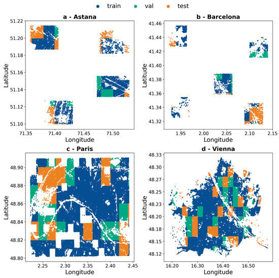
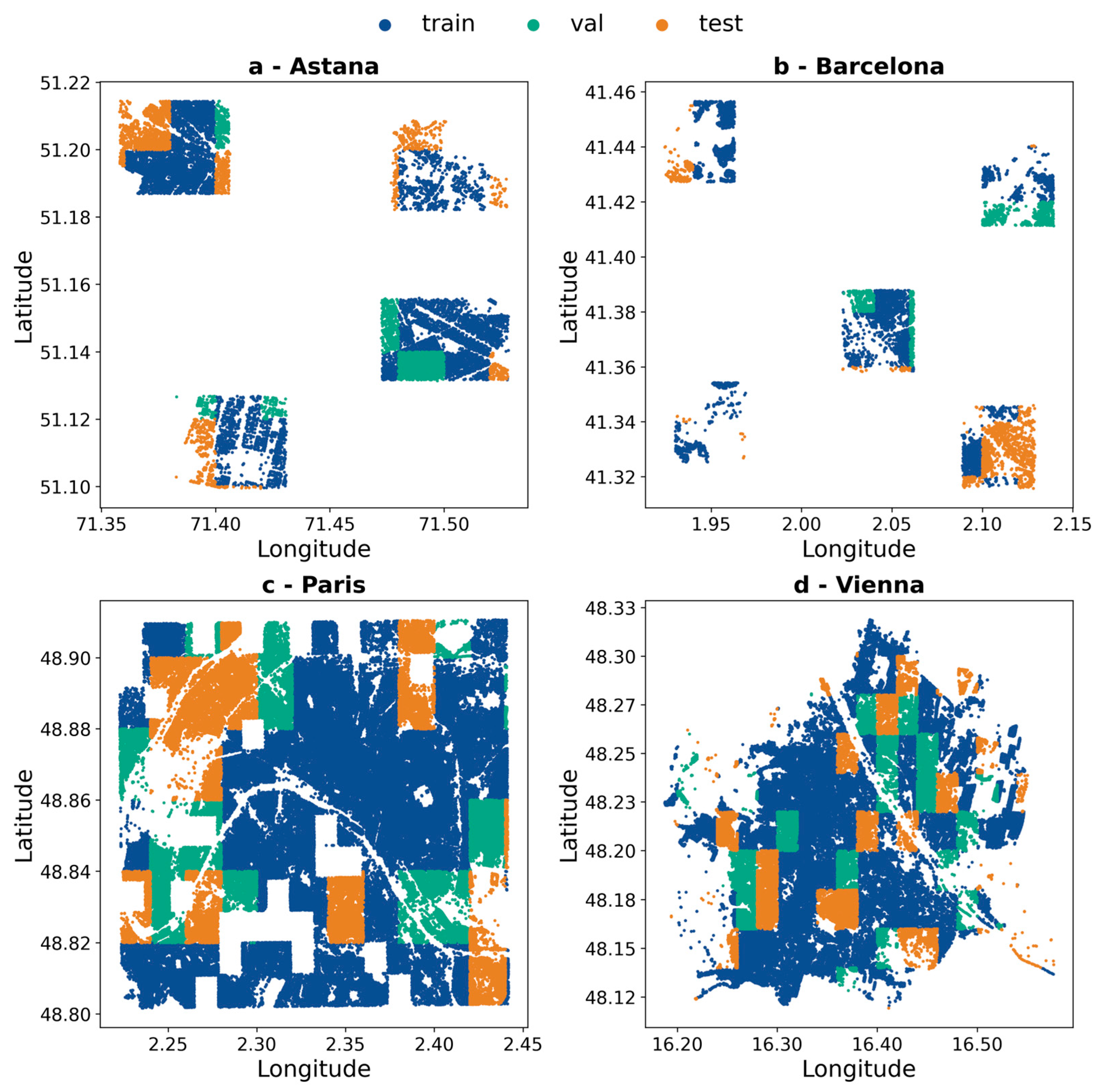
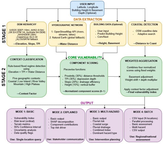
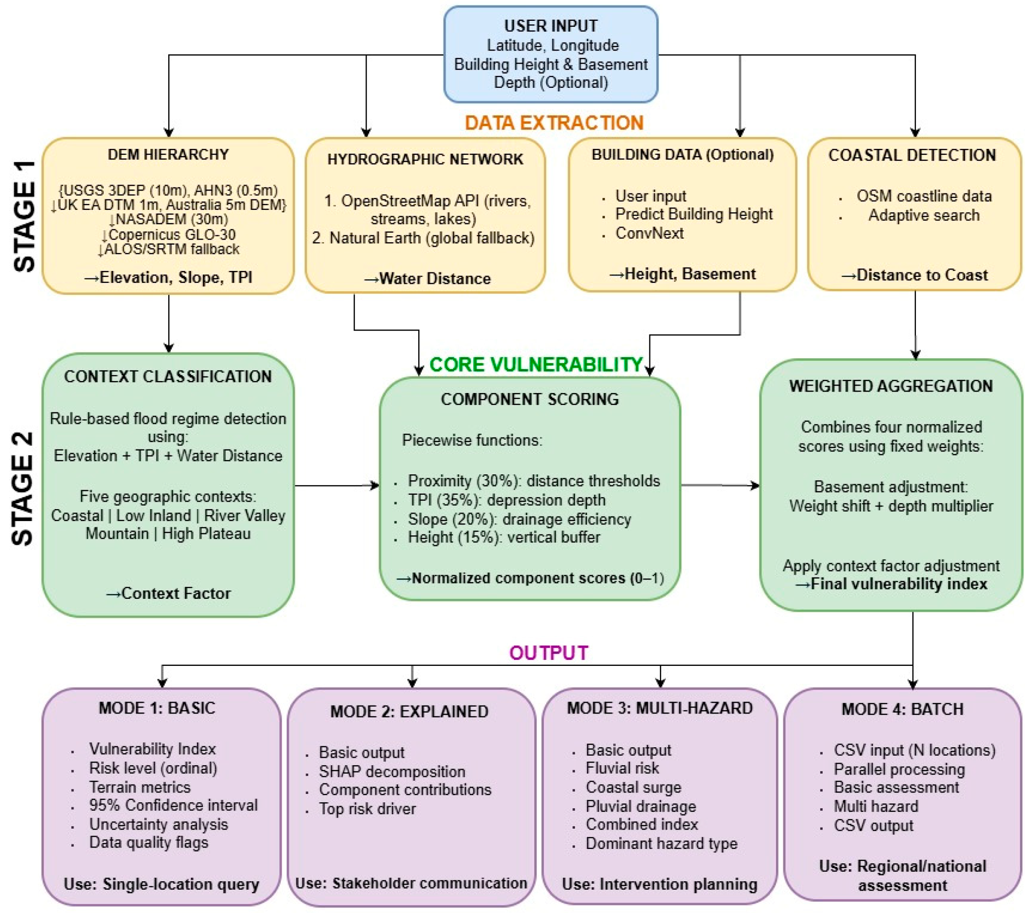
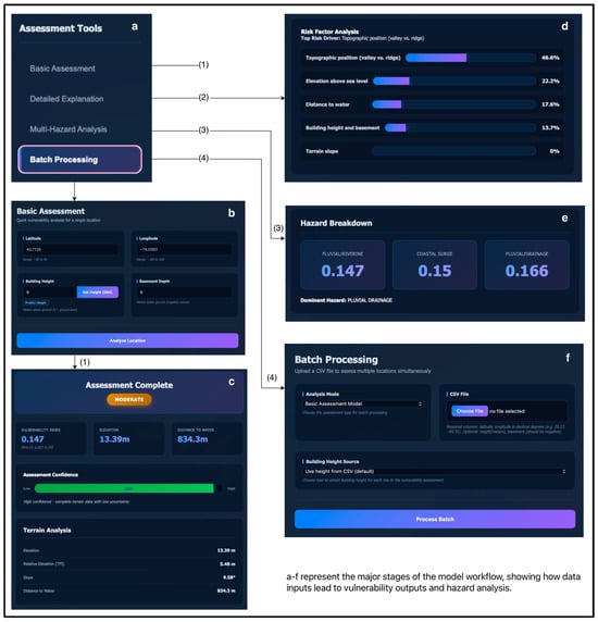
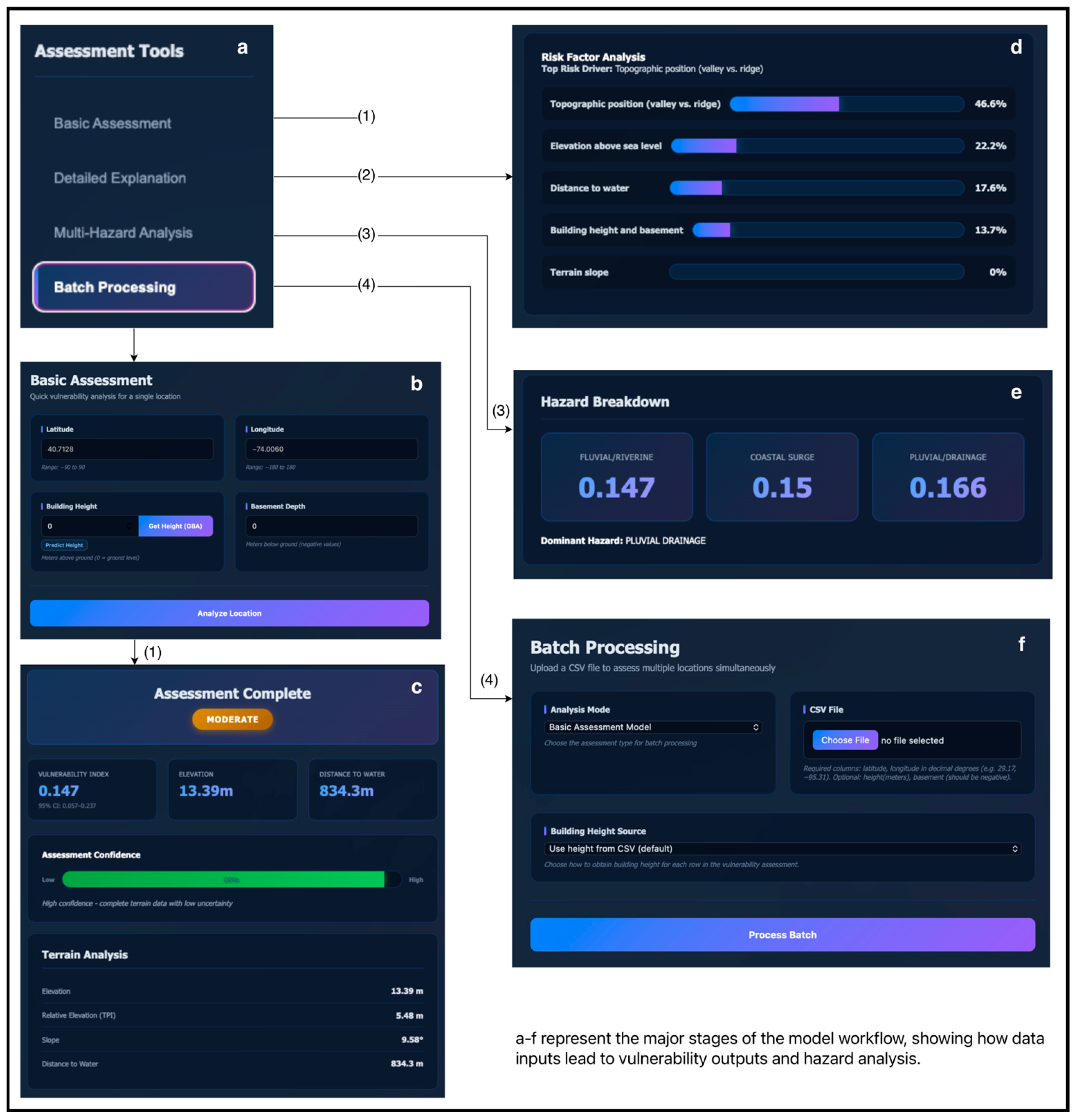
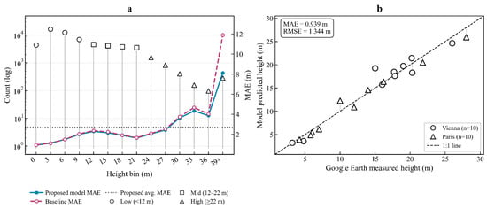
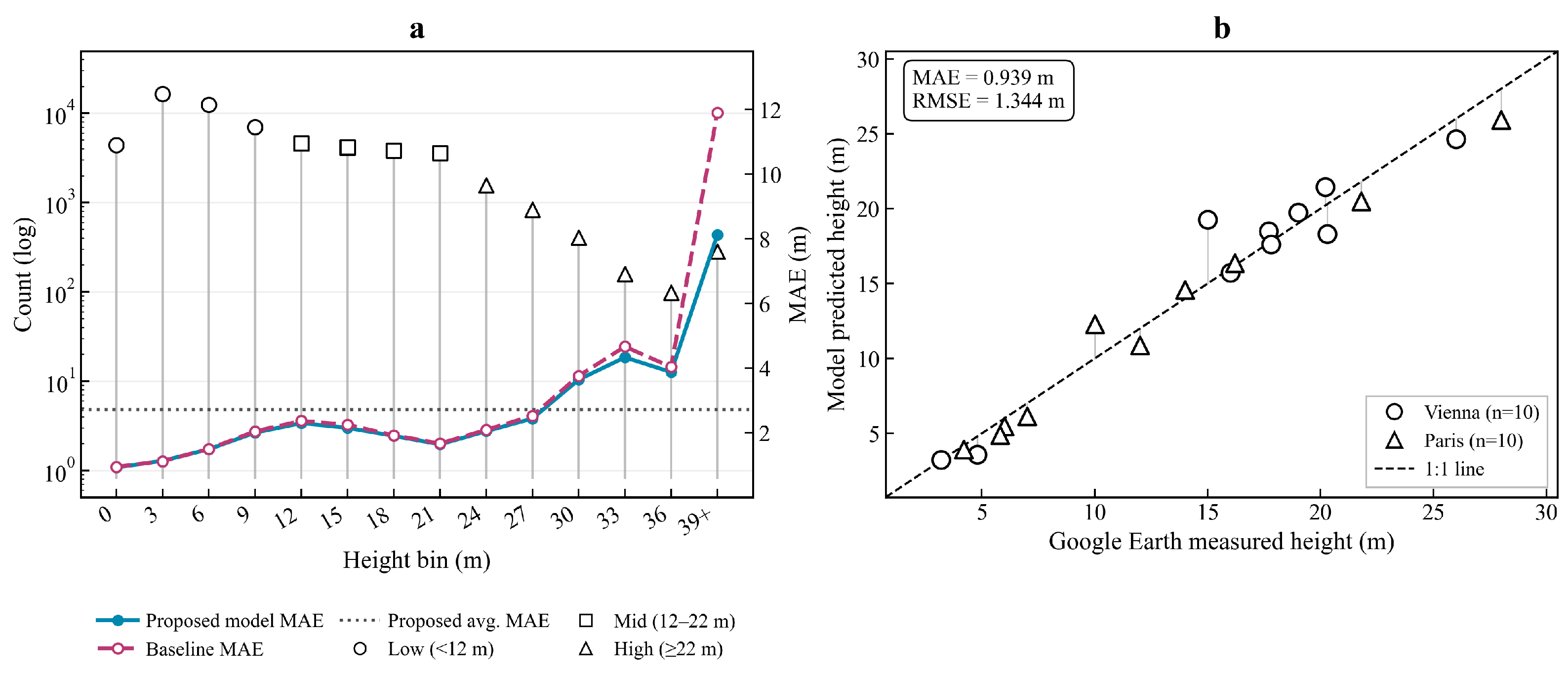
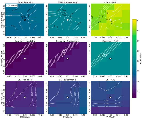
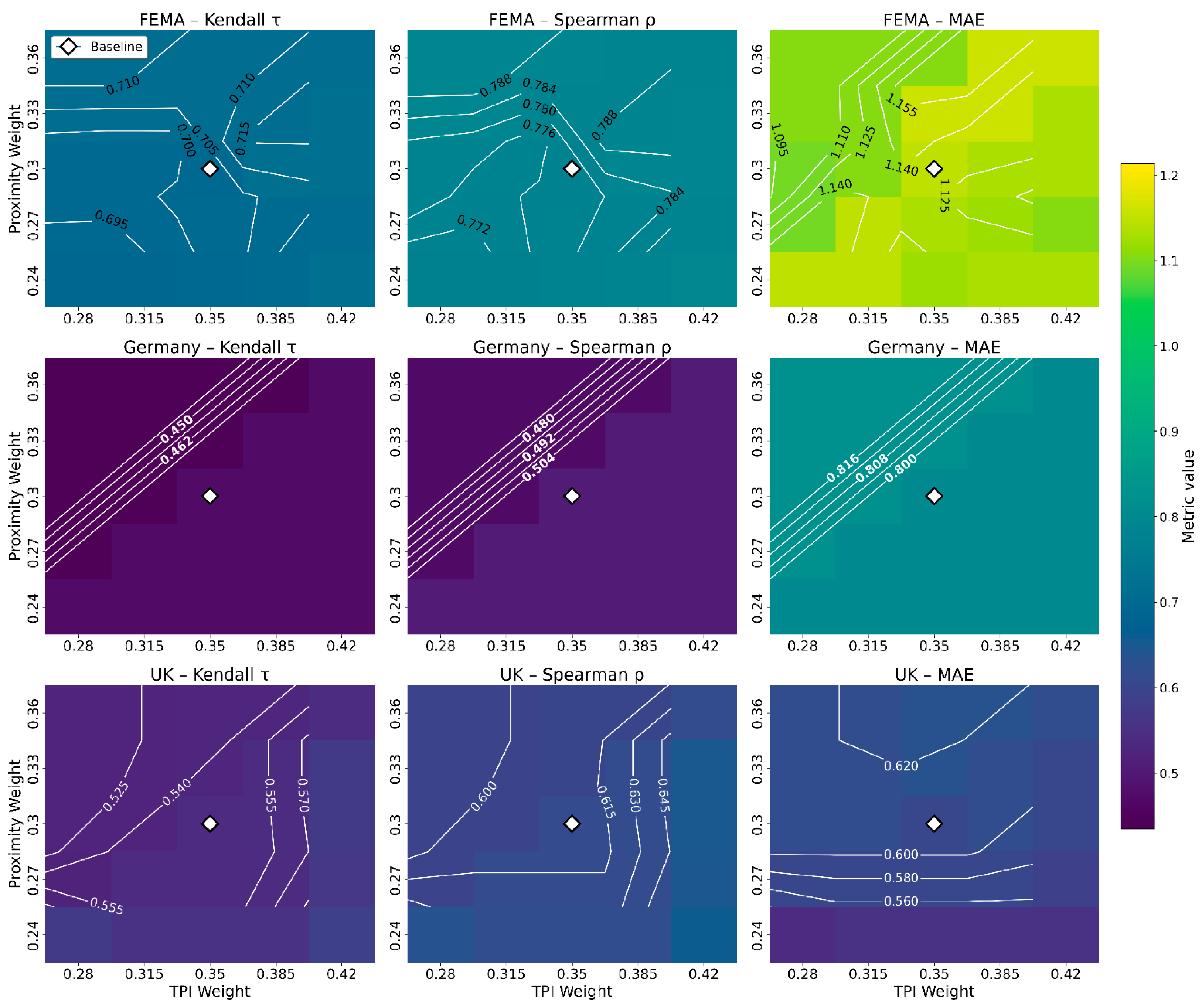
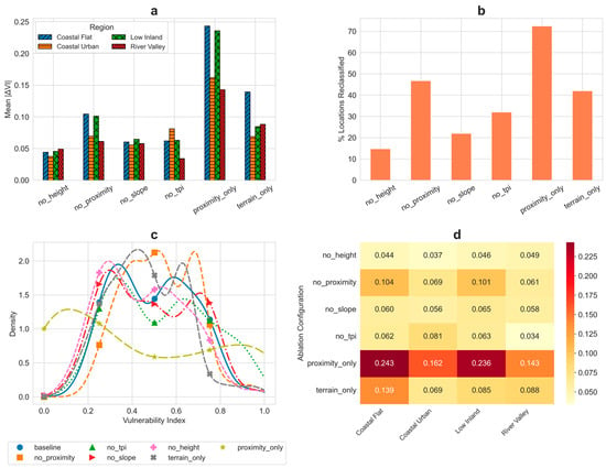
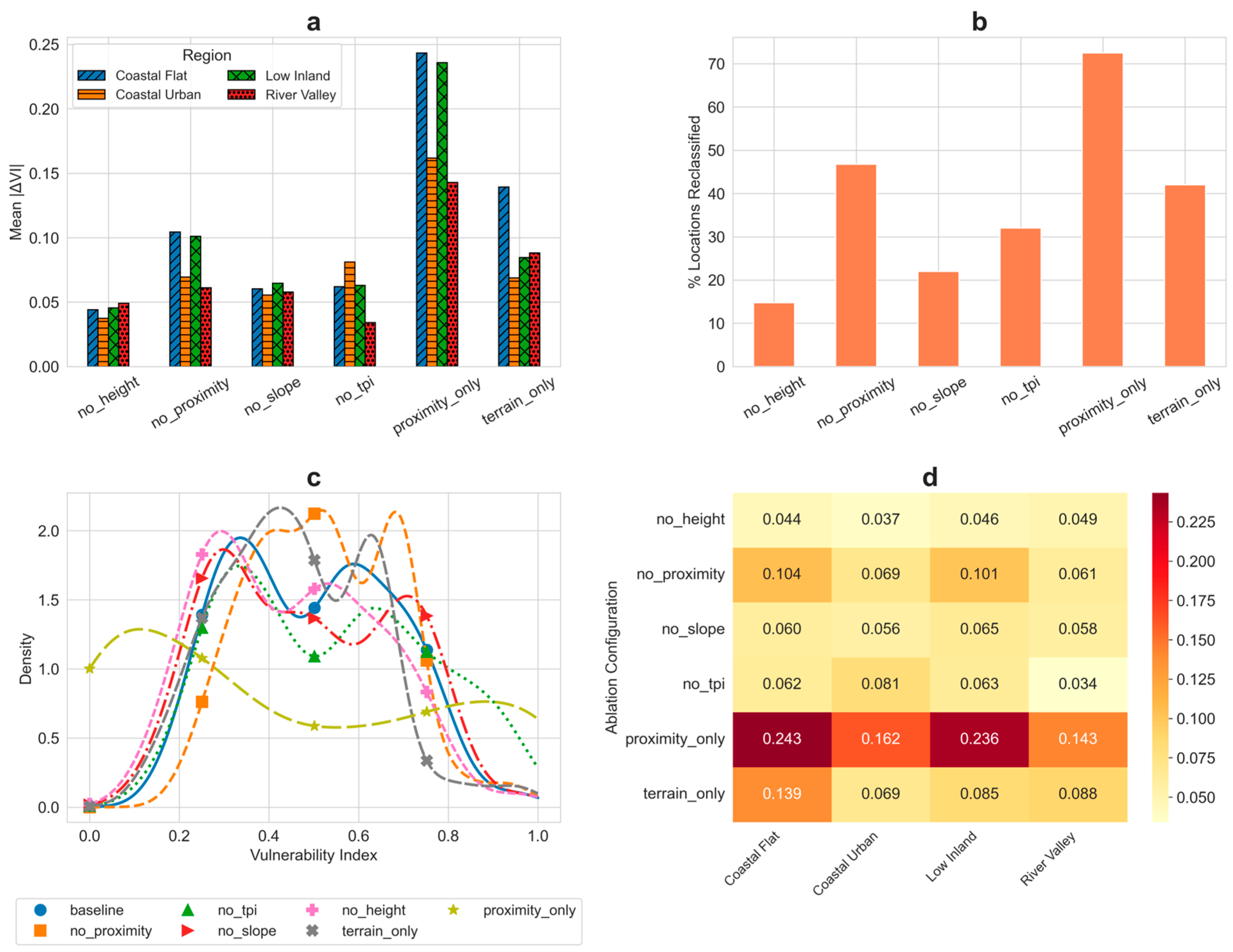
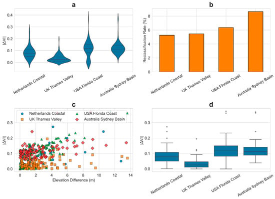
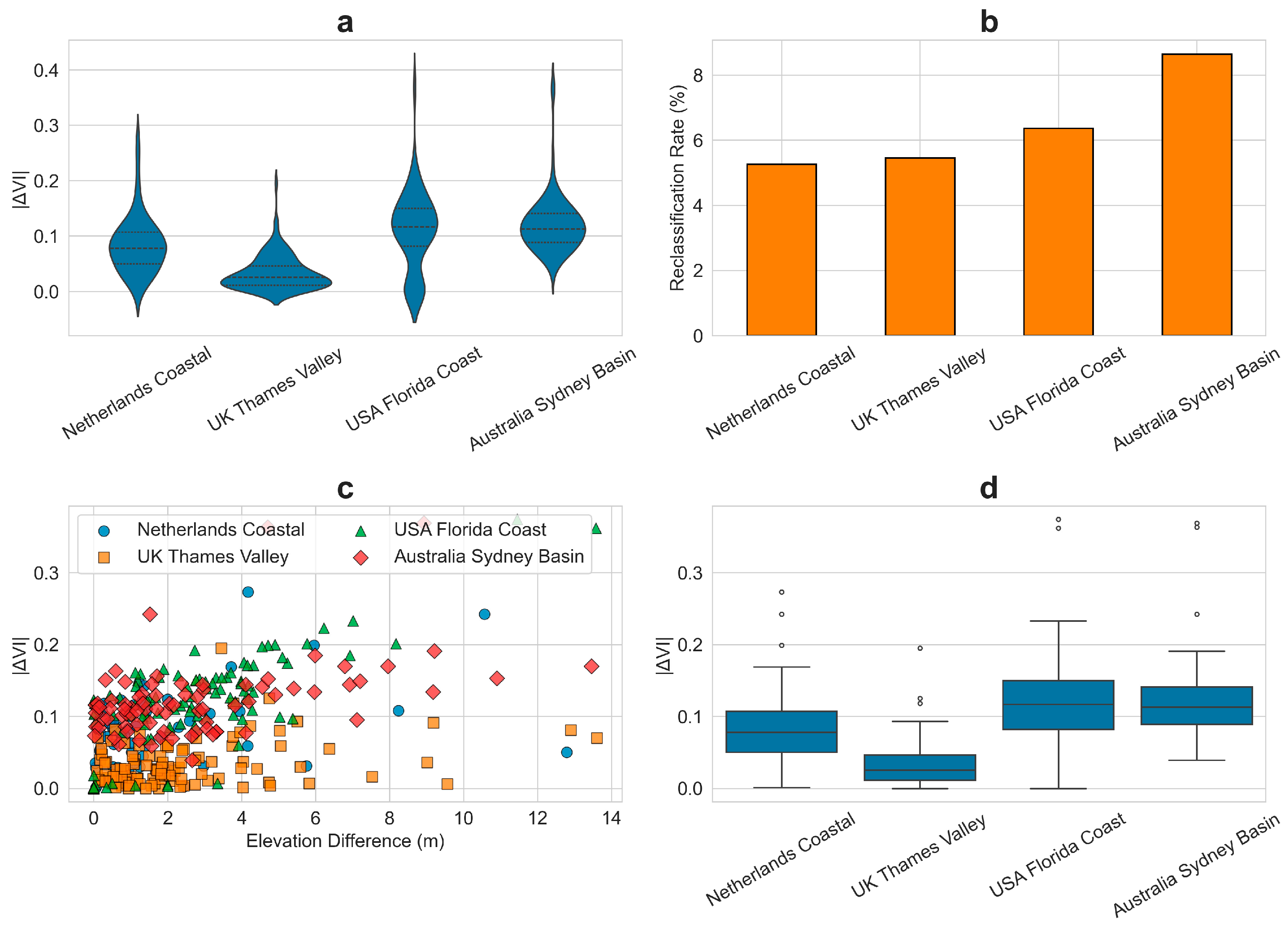
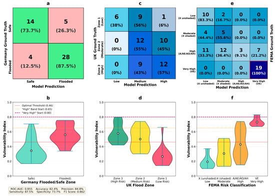
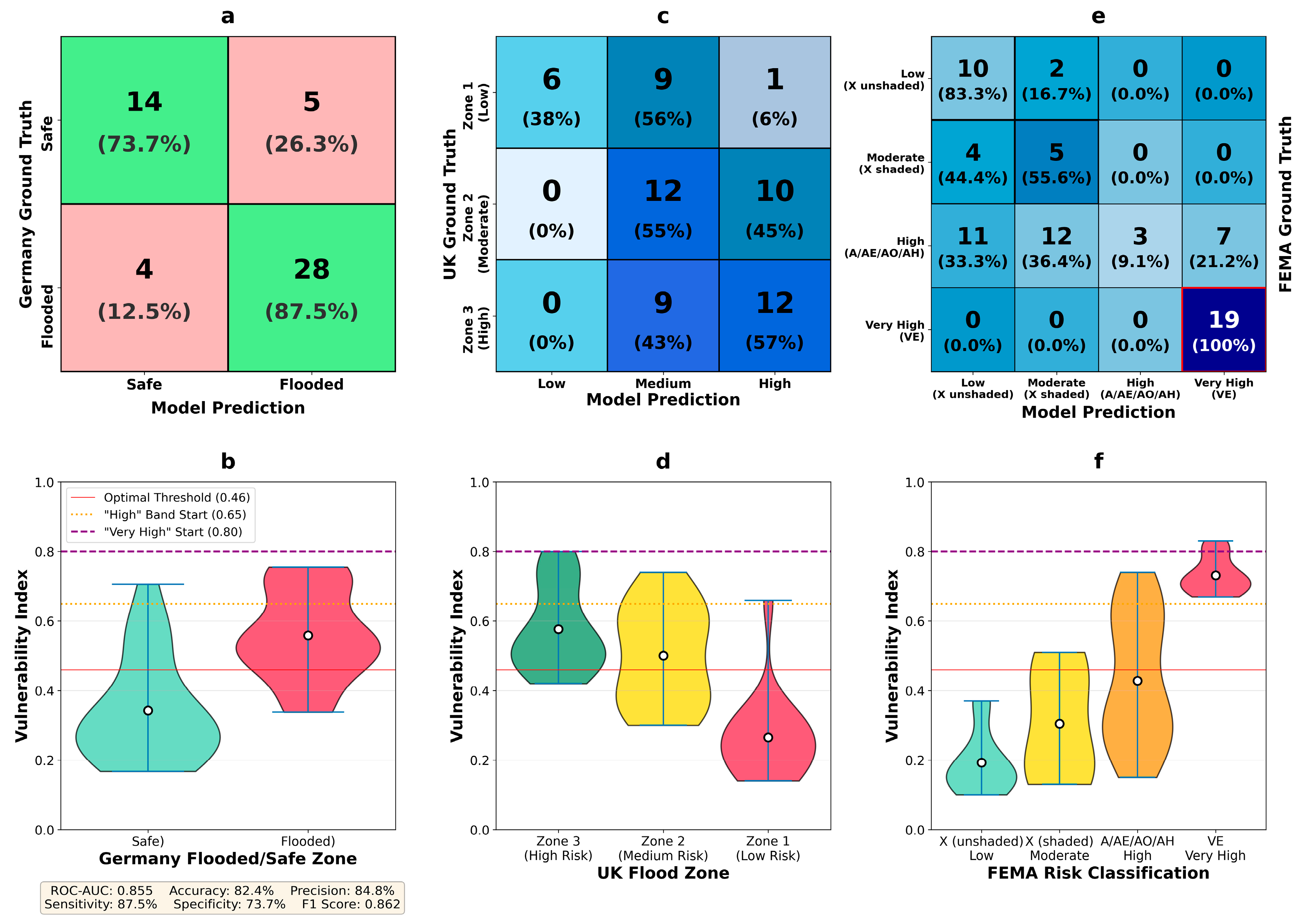
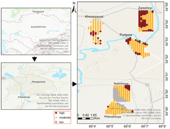
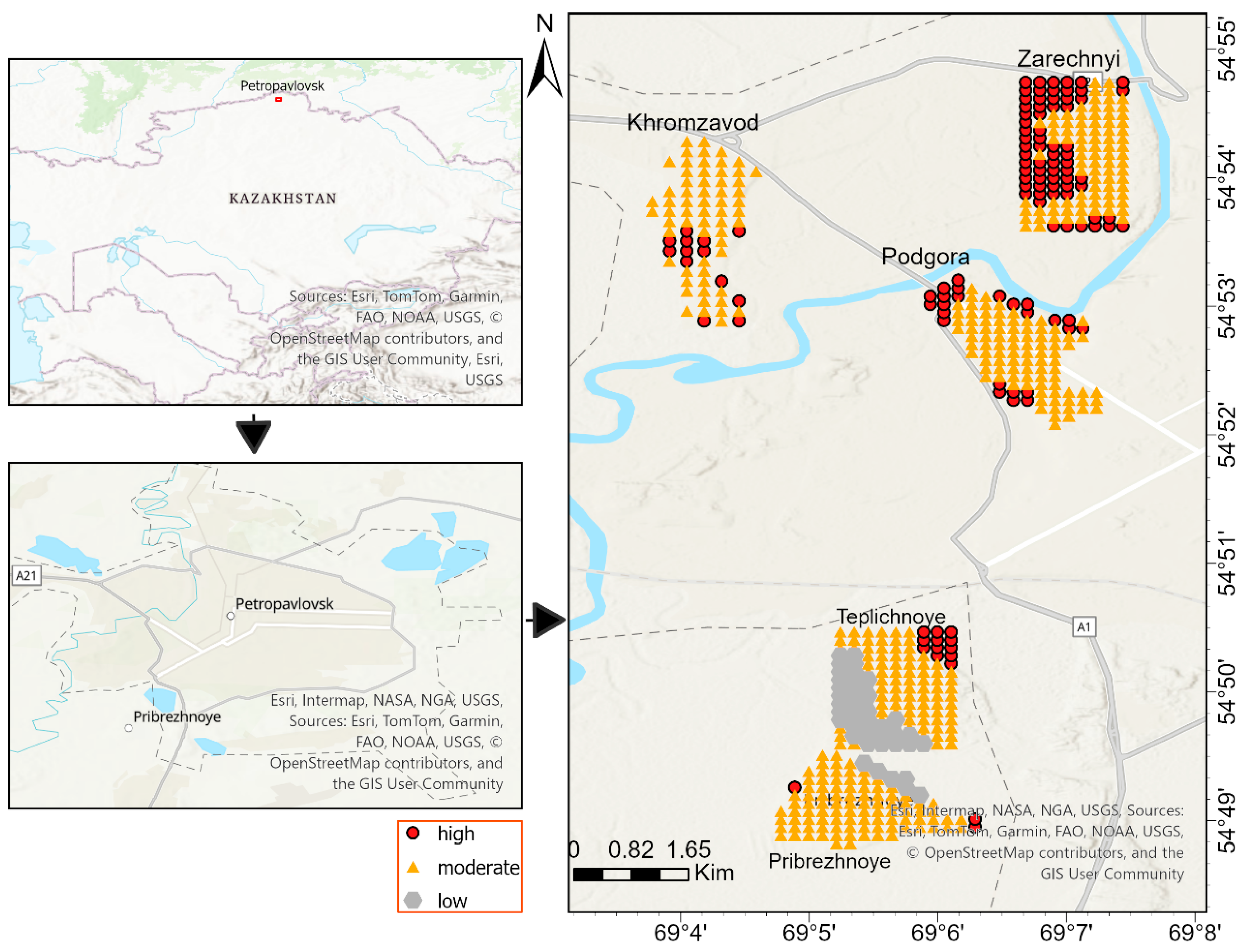

Disclaimer/Publisher’s Note: The statements, opinions and data contained in all publications are solely those of the individual author(s) and contributor(s) and not of MDPI and/or the editor(s). MDPI and/or the editor(s) disclaim responsibility for any injury to people or property resulting from any ideas, methods, instructions or products referred to in the content. |
© 2026 by the authors. Licensee MDPI, Basel, Switzerland. This article is an open access article distributed under the terms and conditions of the Creative Commons Attribution (CC BY) license.