


Highlights
What are the main findings?
- This paper presents a UAV orthophoto-generation-oriented 3D Gaussian Splatting pipeline that can produce orthographic and true-orthographic image outputs under single-GPU constraints. The pipeline targets common urban failure cases, including specular reflection, weak texture, and occlusion, and may alleviate selected artifacts that are often associated with DSM-based occlusion handling in conventional workflows.
- A structure-aware density control scheme (DS-ADC) is introduced, combining a Concentric Topological Neighborhood Atlas (CTNA) with Edge-weighted Dynamic Consistency Scoring (E-DynaCons). CTNA filters gradients within a structured neighborhood, while E-DynaCons assigns higher densification priority to regions with consistent edge observations. Together, these two components steer densification toward reliable regions and suppress boundary over-densification and floating artifacts.
- An orthographic tiled rendering + stitching strategy with a “core–buffer” dual-layer tile mechanism and overlap-weighted blending is proposed, reducing tile-boundary truncation, seams, and radiometric discontinuities in large-format outputs.
What are the implications of the main findings?
- Provides a lower-cost and hardware-efficient route for 3DGS-based UAV orthophoto/true-orthophoto generation on limited hardware, offering potential support for remote-sensing mapping workflows rather than replacing established photogrammetric production pipelines.
- Improves the usability of 3DGS outputs for orthophoto-oriented applications by reducing common artifacts, such as holes, ghosting, and seams, at the rendering-and-stitching stage.
- Provides a product-level evaluation pathway against commercial photogrammetry software, such as MetaShape and Pix4DMapper, under geo-aligned conditions, supporting geometric-consistency analysis in addition to visual assessment.
Abstract
Unmanned Aerial Vehicle (UAV) orthophoto generation in complex environments remains challenging because weak textures, reflective surfaces, occlusions, and large scene extents can cause incomplete reconstruction, ghosting, and seam artifacts. Although 3D Gaussian Splatting (3DGS) offers an efficient explicit scene representation, its use in large-scale UAV orthophoto generation is limited by high memory consumption, unstable densification, and insufficient support for mapping-oriented orthographic rendering. This paper proposes a single-GPU 3DGS framework for UAV orthophoto generation by integrating adaptive spatial block partitioning, deterministic structure-sensitive adaptive density control, and core–buffer tiled orthographic rendering with weighted blending. The proposed framework decomposes large scenes into resource-bounded subregions, guides Gaussian densification using fixed multi-view neighborhoods and edge-enhanced dynamic consistency, and generates large-format orthophotos with reduced boundary and seam artifacts. Experiments on MatrixCity-S and multiple UAV photogrammetric datasets show that the method achieves competitive reconstruction quality and improved resource efficiency. On MatrixCity-S, it reaches 29.01 dB PSNR and 0.901 SSIM, while completing training in 1 h 49 min on a single NVIDIA RTX 3090 GPU. Compared with BlockGS, peak VRAM consumption is reduced by more than 38% across datasets. Under geo-aligned comparison conditions, line-measurement comparisons with MetaShape and Pix4DMapper yield RMSE values of 0.099 m and 0.087 m, respectively. These results demonstrate the potential of the proposed framework for memory-efficient 3DGS-based UAV orthophoto generation under constrained hardware resources, while further control-point-based validation is still needed for rigorous surveying-grade applications.
1. Introduction
Low-altitude UAV remote sensing has become an important tool for urban management, disaster assessment, engineering surveying, and digital-twin applications. Its main mapping products include digital orthophoto maps (DOMs), true digital orthophoto maps (TDOMs), dense point clouds, and 3D models. In practical production, large-area coverage, non-uniform viewing geometry, occlusions, weak textures, and reflective surfaces can cause incomplete reconstruction, ghosting, radiometric inconsistency, and mosaic seams, thereby reducing the usability of DOM/TDOM products. Previous studies have reviewed orthorectification and mosaicking workflows [1], compared explicit-geometry and implicit-representation-based orthophoto generation methods [2], improved radiometric consistency through normalization and block adjustment [3,4], and evaluated mapping accuracy using ground control points, check points, RMSE, and related geometric indicators [5,6]. Occlusion handling and building-oriented reprojection strategies have also been investigated to improve roof completeness and reduce ghosting artifacts [7,8]. However, robust and efficient orthophoto generation in weak-texture, reflective, and structurally complex UAV scenes remains challenging.
Recent advances in 3D Gaussian Splatting (3DGS) [9] provide an explicit and differentiable representation with fast GPU rasterization, making it attractive for large-scale scene reconstruction and remote-sensing mapping. Surveys have summarized progress in optimization, rendering acceleration, compression, and downstream applications, while also identifying scalability, training stability, and reproducibility as open issues [10,11]. For large-scale reconstruction, CityGaussian [12], CityGaussianV2 [13], DOGS [14], BlockGaussian (BlockGS) [15], and related tile-consistency studies [16] have explored divide-and-conquer training, geometric constraints, distributed optimization, single-machine processing, and inter-block consistency. In remote-sensing scenarios, AGS [17], DroneSplat [18], ARSGaussian [19], and EOGS [20] further demonstrate the potential of Gaussian representations for aerial, UAV, LiDAR-assisted, and satellite photogrammetric applications. Recent work has also begun to connect 3DGS with DOM/TDOM generation [21], including orthographic Gaussian projection for TDOM production [22], engineering-oriented orthophoto studies [23], and sparse-view orthophoto generation with structural priors [24]. These studies show that 3DGS is being explored beyond novel-view synthesis toward orthophoto-oriented outputs, but several practical issues remain unresolved for UAV orthophoto production under constrained hardware.
Despite these advances, three issues limit the direct use of 3DGS for UAV orthophoto generation. First, large UAV surveys usually contain hundreds or thousands of high-resolution images, and unconstrained Gaussian densification can rapidly increase model size and GPU memory consumption, making stable single-GPU training difficult. Second, weak textures, repetitive patterns, reflective surfaces, and non-uniform viewpoints can make photometric gradients unreliable, leading to erroneous densification, floating artifacts, texture streaking, or local geometric degradation. Third, even when a 3DGS model is successfully reconstructed, producing large-format orthographic image products still requires a practical rendering and mosaicking protocol that controls tile-boundary artifacts, seam visibility, sampling distance, coordinate consistency, and product-level comparison with photogrammetric outputs.
To address these issues, this paper proposes a UAV orthophoto-oriented 3DGS framework that integrates adaptive spatial block partitioning, deterministic structure-sensitive adaptive density control, and core–buffer tiled orthographic rendering. The framework is designed to enable stable reconstruction of large UAV scenes on a single GPU, guide Gaussian densification toward structurally reliable regions, and generate visually continuous orthographic mosaics suitable for product-level comparison and geometric-consistency assessment.
The main contributions of this study are summarized as follows:
(1) An Adaptive Spatial Block Partitioning (ASBP) strategy is developed to decompose large UAV scenes according to spatial point distribution and view-coverage constraints, enabling scalable 3DGS reconstruction under single-GPU memory limits.
(2) A Deterministic and Structure-sensitive Adaptive Density Control (DS-ADC) scheme is proposed by combining a Concentric Topological Neighborhood Atlas (CTNA) with Edge-aware Dynamic Consistency Scoring (E-DynaCons), allowing densification and pruning to focus on structurally meaningful regions while suppressing redundant or floating Gaussian primitives.
(3) A core–buffer tiled orthographic rendering and weighted mosaicking strategy is designed for large-format UAV orthophoto generation, reducing tile-boundary truncation, seam artifacts, and radiometric discontinuities. The generated orthographic products are compared with representative 3DGS baselines and commercial photogrammetric software outputs under consistent alignment conditions.
2. Methodology
2.1. Overview
This section presents a framework for large-scale 3D reconstruction and orthophoto generation in UAV remote-sensing scenes under a single-GPU setting. The framework is built around a deterministic, structure-aware adaptive density control (ADC) scheme, termed DS-ADC (Deterministic and Structure-aware ADC). To enable deployment in large and complex geospatial environments, an optimized scene partitioning strategy, Adaptive Spatial Block Partitioning (ASBP), is introduced. This section details two key components of DS-ADC: (1) the Concentric Topology Neighbor Atlas (CTNA), which provides multi-view geometric correlation information; and (2) the Edge-aware Dynamic Consistency Scoring (E-DynaCons), which defines an edge-aware, structure-driven error metric. Their roles in guiding densification are described in detail. Finally, the procedure for generating a visually consistent and scale-controlled orthographic tile mosaic from the trained 3D Gaussian splatting model is presented.
The overall framework is illustrated in Figure 1. Subfigures A–C correspond to three sequential stages: subregion partitioning, partition-wise training, and orthographic image generation. Together, these stages form an integrated pipeline for high-quality large-area reconstruction and orthographic product generation under a single-GPU hardware constraint.
Figure 1.
Overview of the proposed method. (A) Partitioning stage. (B) Training stage. (C) Orthophoto generation stage.
2.2. Adaptive Spatial Block Partitioning
Deploying 3DGS in large-scale remote-sensing scenarios, such as city-scale environments or wide-area terrain mapping, introduces challenges that differ substantially from those encountered in small-scale scene reconstruction. These challenges stem primarily from rapid growth in data volume and the characteristics of geospatial datasets. First, computational resource constraints become a dominant limitation. A large scene may comprise thousands to tens of thousands of high-resolution images. The associated initial sparse point cloud (typically produced by SfM) can contain millions to tens of millions of points. Loading the entire scene at once and initializing it as a single 3DGS model can impose GPU memory and CPU RAM requirements that exceed the capacity of typical workstations. Second, optimization efficiency and convergence behavior become key issues. Jointly optimizing a massive model with on the order of hundreds of millions of parameters leads to prohibitively long training times and increases the risk of convergence to suboptimal local solutions. Moreover, gradient propagation over large spatial extents can be inefficient, resulting in highly uneven convergence across different regions of the scene. Finally, scalability through parallelization and workflow robustness are important in practice. For large-scale 3DGS reconstruction, the ability to decompose the task for distributed computation, while ensuring that failures in individual subtasks do not compromise the overall pipeline, is a key engineering consideration. In resource-constrained settings, a sequential strategy that trains subregions independently and then fuses their results can provide a practical solution.
The proposed framework assumes that an initial SfM reconstruction is available, including sparse 3D points and camera poses with sufficient global consistency. These SfM outputs provide the geometric basis for spatial partitioning, view assignment, Gaussian initialization, and orthographic ROI determination. Therefore, the quality of the initial SfM reconstruction inevitably affects the final orthophoto. In practice, local point-cloud noise or a small number of outliers can be partly alleviated by outlier removal, visibility weighting, quantile-based ROI trimming, and the view-coverage constraint used in ASBP. However, these mechanisms cannot fully compensate for severe SfM failures, such as large pose drift, missing reconstruction over extended areas, or highly inconsistent sparse points. In such cases, the resulting Gaussian reconstruction and the derived orthophoto may inherit the corresponding geometric defects.
Conventional scene-partitioning strategies, such as fixed-size geographic gridding or standard octree subdivision, can segment the space. However, they often ignore terrain and surface characteristics and thus struggle with the highly non-uniform data distribution in large, complex scenes. For instance, a grid cell may fall largely within low-texture water surfaces or vegetation regions, yielding few usable SfM points and thereby degrading 3DGS reconstruction quality. In contrast, a neighboring cell may span a structurally complex building, which can demand a substantially higher computational budget than average to model and train effectively.
To address the above issues, this paper builds upon prior work and adopts an Adaptive Spatial Block Partitioning (ASBP) strategy. A data-driven recursive bisection procedure decomposes a large-area scene into independent sub-scenes. Each sub-scene remains within a bounded resource budget and maintains adequate view coverage. This decomposition enables 3DGS training on consumer-grade single-GPU hardware.
The key idea of ASBP is to recursively and adaptively split the scene point cloud based on its 2D ground-plane projection. Unlike simple midpoint splitting or K-means clustering, ASBP determines partition boundaries jointly from the spatial distribution of 3D points and the associated view-coverage characteristics of the scene.
2.2.1. Ground-Plane Projection with Visibility Weighting
After outlier removal and Manhattan alignment, the first step of ASBP projects the sparse 3D point cloud onto a 2D ground plane. This preserves the horizontal spatial distribution of the scene. Meanwhile, ASBP assigns each sparse point a visibility weight . In SfM, a point observed by more cameras and with a smaller mean reprojection error is typically estimated more accurately and more stably in 3D. Accordingly, the visibility weight is defined as a function of the observation count and the reprojection error:
Here, denotes the number of cameras (i.e., views) in which point is observed, and denotes the mean reprojection error of . In subsequent partitioning decisions, this weighting assigns greater influence to reliable feature points that provide stable structural support for the scene.
2.2.2. Recursive Subdivision via Weighted-Median Splitting
After the first step, ASBP performs region splitting in a recursive manner. It takes the 2D axis-aligned bounding rectangle of the projected scene as input and determines whether further subdivision is required based on a set of partitioning constraints. Specifically:
- Initial boundary. First, the algorithm computes the minimum-area bounding rectangle (MABR) that encloses all projected points. Compared with an axis-aligned bounding box (AABB), the MABR more tightly encloses elongated or irregular scenes with arbitrary orientations. This reduces unused area in the initial processing domain.
- Splitting-axis selection. At each recursion, the longer side of the current rectangle is chosen as the splitting axis . This choice biases the subdivision toward partitions with more balanced aspect ratios, which is beneficial for maintaining workload balance in subsequent training.
- Weighted-median splitting. Instead of a geometric midpoint split, ASBP selects the split location as the weighted median of the point coordinates projected onto the splitting axis . Formally, for any projected point within the rectangle, its coordinate along the splitting axis is , where is the 2D point coordinate and is a reference vertex of the MABR. The cut position is defined such that the sum of weights of points with projected coordinates smaller than is approximately half of the total weight:
Under this formulation, partition boundaries are biased toward regions with lower point density or less reliable geometry, so that structurally coherent or feature-rich areas are more likely to remain within the same subregion. This reduces the risk of partition-induced structural fragmentation.
2.2.3. Constraints for Partitioning
Partitioning constraints constitute the key elements of this part. The following three constraints are adopted:
- Point-cloud budget constraint. The number of sparse point clouds contained in a subregion does not exceed the preset upper limit . This constraint condition will directly relate to the GPU video-memory requirement at 3DGS initialization, and is the core for ensuring task startup.
- View-coverage constraint. To ensure that each subregion has sufficient viewpoint constraints, the camera views assigned to the subregion as constrained. First, the number of views must be no less than the lower bound . Second, a refined coverage criterion is used to filter candidate views. Specifically, for a candidate view , the algorithm computes two ratios: (1) the fraction of points in subregion observed by relative to the total number of points in (subregion coverage ratio ); and (2) the fraction of points in subregion among all points observed by (view coverage ). A view is assigned to subregion only if the following conditions are satisfied:Here, denotes the coverage threshold (e.g., 0.3). The logical “or” ensures selection of two types of views. The first type covers a large portion of the subregion. The second type may observe only a limited part of the subregion, but the subregion accounts for a large fraction of the view’s observed content.
- Recursion-depth constraint. To avoid excessive subdivision that would create many tiny fragments with insufficient texture, a maximum recursion depth is imposed. This constraint keeps each subregion at a reasonable spatial extent and helps maintain a manageable computational budget while still ensuring adequate training-view availability.
Figure 2 shows the workflow of ASBP. After recursion ends, each leaf rectangle that satisfies the constraints is treated as an independent subregion. For each subregion, an anisotropically expanded 3D bounding box is constructed. It is extended more along the vertical axis to include complete rooftop structures and reduce boundary truncation effects across neighboring subregions. Based on the camera geometry assigned to the subregion, the corresponding initial point set is extracted, which provides reliable training data for the subsequent DS-ADC framework.
Figure 2.
Overview of adaptive spatial partitioning workflow. This figure schematically illustrates the partitioning process, where a complete region is divided into four subregions, distinguished by four different colors.
2.3. Improved Adaptive Density Control Scheme
In standard 3DGS, scene fidelity is progressively improved by alternating between parameter optimization and density control (i.e., densification and pruning), which aims to increase geometric detail and visibility coverage. The densification schedule typically depends on the randomly sampled training views and is triggered by image-domain photometric losses together with several heuristic statistics (e.g., position-parameter gradients, opacity, and scale). However, in scenes with complex textures, large scale variation, or non-uniform camera distributions, this paradigm exhibits two key limitations [25]. First, the density-control signal can be highly sensitive to the sequence of online view sampling. Under different sampling orders, the same structure may be densified at different times and with different intensities. Second, photometric residuals alone may not reliably localize structurally misaligned regions. These residuals can be confounded by texture-phase differences, exposure changes, and other appearance variations. In turn, this confusion may lead to unnecessary densification or redundant primitives.
Motivated by these issues, this paper proposes a Deterministic and Structure-aware Adaptive Density Control scheme (DS-ADC) to improve the robustness of densification signals and enhance sensitivity to structure-related errors. Without modifying the primary 3DGS optimization loop, DS-ADC introduces a joint constraint that combines multi-view context with structure-aware pixel masks. Specifically, an offline, precomputed Concentric Topology Neighbor Atlas (CTNA) provides a fixed neighborhood set for each reference view. Given this neighborhood, Edge-aware Dynamic Consistency Scoring (E-DynaCons) produces a structure-informed, pixel-wise binary map. The resulting pixel masks are aggregated into primitive-level coverage statistics via the rendering coverage relationship between pixels and contributing Gaussian primitives. These statistics provide additional criteria for densification and for setting pruning weights. As a result, DS-ADC suppresses erroneous densification driven by texture and sampling fluctuations, while balancing reconstruction quality against computational cost.
2.3.1. Overall Pipeline
Let the training camera set be . During a densification step, the training procedure selects a reference view . CTNA then returns a neighborhood set of size , denoted . For each neighboring view , a binary metric map (i.e., a pixel domain mask) is computed. The mask is aggregated via pixel-to-primitive coverage relationships in the rendering stage and mapped to the Gaussian-primitive level. This yields two scores for each primitive : an importance score and a pruning-propensity score . Finally, is applied as an additional criterion for densification, whereas is used to weight pruning and to determine the hard-pruning threshold in the later stage.
2.3.2. Concentric Topology Neighbor Atlas
In the standard 3DGS formulation, optimization and error metrics are primarily based on per-view photometric reconstruction, without explicitly imposing cross-view constraints or introducing a fixed multi-view context. Consequently, the signals used for density control are often derived from single-view local observations and can be sensitive to texture patterns, occlusions, and stochastic view sampling. Recently, several studies have incorporated multi-view cues during densification, although the goal is typically not to enforce a classical multi-view geometric-consistency constraint; instead, multi-view information is used as an auxiliary reference [26]. Such cues can suppress error-driven over-densification while promoting primitive growth at geometrically reliable locations. Motivated by this idea, the Concentric Topology Neighbor Atlas (CTNA) proposed in this section determines offline a stable and representative set of neighboring views for each reference view, which provides a reliable basis for subsequent densification decisions. Specifically, CTNA uses candidate-selection strategies, including temporal neighbors, geometric neighbors, and ring-based sampling, to define correlation weights based on the distance between camera centers and the angular difference between viewing directions. It then selects a subset of high-weight views to form a fixed neighborhood for each training view. This design aims to balance local consistency with viewpoint diversity.
- Candidate set construction
For a reference view , let the camera center be and the camera’s forward unit viewing direction be . The candidate pool is defined as the union of three sets constructed by different heuristics: (1) temporal neighbors , which are adjacent to in the acquisition sequence; (2) geometric nearest neighbors , selected based on the distance between camera centers; and (3) ring-based sampling , obtained by sorting views by distance and then subsampling at fixed intervals. The three sets are defined as follows:
Here, denotes the -th closest view to the reference view (excluding itself), where the ordering is defined by the distance between camera centers. The parameter is the ring-sampling stride, denotes the number of consecutive cameras selected at each sampling step, indexes the sampled ring, and is the total number of views skipped to avoid overlap with the geometric nearest neighbors and temporal neighbors. Figure 3 provides a spatial illustration of the candidate set for and .
Figure 3.
Schematic diagram of candidate set construction. Triangles denote camera/view positions along a zigzag UAV flight path. The number of temporal (sequential) neighbors is 1, the number of geometric nearest neighbors is 6, the ring-sampling stride is 4 (i.e., three intermediate views are skipped between selected views), and 11 consecutive views are selected at each sampling step (i.e., candidate views).
The union of the three candidate sets is then deduplicated to obtain the final set:
- 2.
- Adaptive geometric weighting with a deterministic neighborhood
For any candidate view , the distance between camera centers is defined as follows:
as well as the angular difference , defined via . A correlation weight can then be defined as follows:
Here, and control the distance-based and view-direction (camera orientation) penalty terms, respectively. Equation (9) employs a separable, monotonic penalization, such that distance and orientation independently down-weight the correlation score. This design prevents extreme values in one term from overwhelming the contribution of the other, thereby maintaining a balance between local proximity and viewpoint diversity. To accommodate scenes at different spatial scales, the distance penalty is normalized using the median of the global nearest-neighbor distances:
denotes the index of the nearest neighboring view of (under the camera-center distance). The neighborhood atlas is then constructed by selecting the candidate views with the highest correlation weights:
Because is computed offline and is queried (rather than updated) during training, the resulting neighborhood is deterministic and fully reproducible for a given reference view, providing a stable context for subsequent multi-view statistics. In addition, is set to 0.25 by default. This setting preserves a degree of viewpoint diversity while preventing excessively large orientation differences from dominating neighborhood selection.
2.3.3. Edge-Aware Dynamic Consistency Scoring
Pixel-wise photometric residuals do not necessarily provide a reliable indicator of geometric error. In high-frequency texture regions, even minor appearance variations can substantially amplify residual magnitudes. In contrast, in low-texture areas, pronounced geometric misalignment may elicit only a weak photometric response [27]. Accordingly, E-DynaCons introduces an edge-sensitive residual filtering mechanism during densification to improve the stability of ADC under complex texture and structural conditions. Specifically, CTNA is used to select, for the current view , a neighborhood set comprising highly correlated views (with in this work, as shown in Figure 4, the current view id = 421 is taken as an example from the Factory dataset at the 7000th iteration). Over this set, a normalized L1 residual is computed and fused with edge cues extracted from the reference image to produce a pixel-wise binary map. This map preserves high-residual regions and amplifies residuals near edges. As a result, selected pixels are biased toward contours and boundaries that better reflect geometric structure.
Figure 4.
Illustration of the current view (id = 421) and its neighboring view set.
After the pixel-wise binary metric maps are obtained, the pixel-domain signals must be transferred to the Gaussian-primitive level to guide densification decisions. Accordingly, E-DynaCons projects each Gaussian primitive onto the image plane of each neighboring view. For each view, it counts the positively labeled pixels in the metric map that fall within the projected footprint. The counts are summed over the neighborhood set to form a primitive-level score. A score greater than zero indicates that the primitive contributes, in at least one neighboring view, to imaging a region flagged as structurally inconsistent. Such primitives are added to the densification candidate set. With this constraint, densification can better separate structure-related errors from appearance-driven residuals in complex textured areas. This encourages suitable primitive growth while reducing redundant or uninformative primitives.
- Binary metric map computation
For view , let the reference (target) image be and the rendered image at training step be . The pixel-wise L1 residual is computed and normalized to obtain , where denotes a pixel location and denotes the image domain. From , a Sobel edge-magnitude map is extracted. The edge-enhanced score map is then defined as follows:
The dynamic weight is defined using a curriculum-learning strategy [28] and is determined jointly by a curriculum-based schedule and an online feedback term. The training progress is defined as , where denotes the total number of iterations, and the scheduling term is given by the following:
To characterize the relative difficulty of edge regions, an edge-pixel set is defined by thresholding . The mean error over edge pixels and the global mean error are then computed as follows:
The feedback term is defined as follows:
Here, denotes the sigmoid function, and avoids division by zero. When the mean edge error is markedly larger than the global mean error, the feedback term increases, thereby automatically placing greater emphasis on edge regions. Finally, the dynamic weight is obtained via a smooth blending of the schedule and feedback terms:
This curriculum-learning-based dynamic weighting strategy reduces reliance on ad hoc hyperparameter tuning by adapting the weighting automatically as training progresses (via ).
Finally, the binary metric map is obtained by thresholding:
Here, is an empirically chosen threshold and is set to 0.1 in this work. The resulting mask identifies regions associated with structural inconsistency, which subsequently supports the structure-aware mapping from pixels to Gaussian primitives and provides effective guidance for densification. Figure 5 illustrates the workflow for generating the metric map.
Figure 5.
Workflow for generating the binary metric map.
To further illustrate the generation process of the binary metric map, Figure 6 provides a visualization of the intermediate results at the 7000th iteration. First, the error heatmap in Figure 6b depicts the spatial distribution of the initial reconstruction residuals. Then, the edge magnitude map in Figure 6c is used to capture potential structural boundary information. Based on these two cues, the error is reweighted according to Equation (12), yielding the edge-enhanced error map shown in Figure 6d, which increases the sensitivity to regions containing fine structural details.
Figure 6.
Visualization of the intermediate results in the generation process of the binary metric. (a) Ground-truth image, (b) normalized loss heatmap, (c) edge magnitude map, (d) edge-weighted enhanced error heatmap, (e) binary metric map.
Finally, a thresholding operation is applied to obtain the binary metric map in Figure 6e. The resulting map adaptively concentrates on structurally important regions, such as building boundaries and roof edges. This spatial selectivity is achieved through the adaptive weighting mechanism defined in Equation (12), which dynamically adjusts the error weights according to local geometric complexity, thereby enabling a more effective balance between reconstruction accuracy and structural preservation.
- 2.
- Structure-aware mapping from pixels to Gaussian primitives
The binary metric map highlights high-error regions associated with structural inconsistency in a given view. To use this information for densification, the pixel-domain signal must be aggregated to the Gaussian-primitive level. Let the current set of Gaussian primitives be . For any view , the renderer projects each primitive onto the image domain , yielding its 2D footprint under that view. Let denote the coverage indicator of primitive at pixel : if is visible at and contributes non-zero color, then ; otherwise, .
Based on this pixel-level coverage relationship, two counts are defined for each primitive and view: a structural-hit count and a total-coverage count , which are expressed as follows:
For the reference view and its neighborhood set , the multi-view importance score of a Gaussian primitive is defined as the cumulative (summed) structural-hit count over the neighborhood views:
When , the primitive covers, in at least one view within the multi-view neighborhood, pixels that are flagged as exhibiting structurally notable error; thus, is admitted as a candidate for densification.
In addition to guide pruning, a pruning-propensity score is introduced. First, a normalized view-level structural participation rate is defined as follows:
The mean participation rate is computed as , i.e., averaged over the reference view and its neighboring views. The resulting pruning-propensity score is then defined as follows:
When a Gaussian primitive contributes only rarely to regions flagged as structurally inconsistent across multiple views (i.e., is small), the corresponding approaches 1, making it more likely to be removed during pruning. Conversely, when frequently covers structurally inconsistent regions (i.e., is large), decreases, indicating that the primitive remains informative for preserving structural fidelity and should be retained for further optimization.
2.3.4. Densification Guided by Gradient Candidates and Structural Constraints
- Densification
This paper retains the standard 3DGS densification procedure while introducing as an additional structure-aware criterion. The goal is to inject explicit scene-structure cues so that densification is driven by structurally meaningful errors rather than appearance-only artifacts. Let and denote the clone and split candidate sets produced by the original 3DGS. Under the proposed structural constraint, a candidate primitive is admitted to the final densification sets only if , i.e.,
This forms a two-stage selection mechanism. Gradient-based signals primarily reflect local fitting difficulty and change magnitude, and are used to identify candidate primitives for densification. The structural constraint then assesses whether these candidates correspond to structure-related errors. Densification is triggered only when both criteria are satisfied. This design reduces spurious candidates induced by non-structural factors, such as high-frequency texture-phase discrepancies and local exposure inconsistency. As a result, new Gaussian primitives are preferentially allocated to fine-scale structural details rather than to texture overfitting.
- 2.
- Two-Stage Pruning
Stage one operates during densification. In the original 3DGS, a base pruning candidate set is formed using simple criteria (e.g., persistently low opacity or anomalous scale). A subset is removed to control the number of primitives and stabilize training. Building on this mechanism, the proposed method introduces as a priority signal. Given a deletion budget (the maximum number of candidates removed in the current step; set to 50% of in this work), weighted sampling without replacement is performed to preferentially remove primitives with low structural participation.
Specifically, for each candidate , a sampling weight is defined as follows:
where is a numerical-stability constant. Sampling without replacement is then conducted according to to select primitives that constitute the removal set. Because larger indicates lower structural contribution, Equation (25) assigns higher sampling weights to such primitives, increasing their removal priority under a limited budget. The combination of a fixed budget and sampling without replacement also mitigates training instability that could arise from removing all candidates in a single hard-pruning operation.
Stage two is applied near the end of training, after densification has ended. At this point, the model’s geometric coverage and visibility structure are largely stable. The objective of pruning shifts from controlling model growth during training to compressing the final representation. This entails removing clearly uninformative long-tail primitives without substantially perturbing the converged solution. Accordingly, stage two replaces budgeted sampling with hard pruning of two categories of primitives: (1) primitives with persistently low opacity and negligible contribution to color compositing, and (2) primitives whose structural participation remains consistently low within the fixed multi-view neighborhood, resulting in a persistently high pruning-propensity score . Specifically, let denotes the opacity of the n-th Gaussian primitive. The primitive is removed if the following conditions are satisfied:
Here, denotes the final opacity threshold and denotes the high pruning-score threshold. In this work, and . Stage two is complementary to stage one. Stage one performs smooth, budgeted removal. Stage two applies hard-threshold pruning near convergence to eliminate primitives with low contribution or weak structural relevance. The two stages control model size and reduce computational cost.
Figure 7 illustrates the spatial execution distribution of the proposed two-stage joint densification strategy at the 7000th iteration. In the example shown, among approximately 2.31 million Gaussian primitives (Figure 7a), 95,678 are identified by the metric mask as densification candidates (Figure 7b). Subsequent cloning (Figure 7c) and splitting operations (Figure 7d) are performed primarily around these candidate primitives, enabling targeted refinement in structure-sensitive regions and thereby enhancing the representation of local details. During the pruning stage, 936,103 candidate primitives are first selected based on opacity and structure-related parameters (Figure 7e). After the progressive two-stage filtering process, 189,218 redundant primitives are ultimately removed (Figure 7f). In this way, the proposed strategy effectively controls model size while preserving sufficient representation capacity.
Figure 7.
Illustration of the spatial distribution of the execution regions for the densification. (a) Gaussian primitives before pruning. (b) Gaussian primitives represented by the metric mask. (c) Candidate primitives selected for cloning. (d) Candidate primitives selected for splitting. (e) Candidate primitives filtered based on opacity and structure-related parameters. (f) Primitives finally pruned.
2.4. Orthographic Tiled Rendering and Blending
After a high-quality large-scene 3DGS reconstruction is obtained using ASBP and DS-ADC, the next objective is to generate an orthographic image mosaic. Unlike conventional orthophoto production, orthographic rendering with 3DGS does not require terrain products. An orthographic camera model enables direct rendering of an orthographic image for a specified region in a single pass. Related efforts have also been explored in the NeRF literature [22].
2.4.1. Orthographic Reference Frame and ROI Selection
The first step in orthographic image generation is to establish a globally consistent 2D map coordinate system. A global “up” unit vector is defined using the scene’s prior vertical axis (which can be determined from the projection plane in Section 2.2 or set to the Z-axis of a geographic coordinate system). An orthonormal basis spanning the corresponding ground (map) plane is then constructed such that it is orthogonal to . Under this map coordinate system, any 3D world point can be uniquely expressed as follows:
Here, is a reference point in the scene, denote the coordinates of the point on the map plane, and is the height relative to that plane.
To automatically determine the rendering extent, quantile trimming is applied to the projections of the sparse point cloud onto the plane. Specifically, low (e.g., 0.5%) and high (e.g., 99.5%) quantiles are computed for the distributions of and , and these quantiles define the boundary of the Region of Interest (ROI). Compared with using the minimum and maximum values directly, this strategy is reliable to a small number of spatial outliers introduced during SfM. The resulting rendering region is tighter and more reasonable.
2.4.2. Core–Render Two-Level Tiling Strategy
For a large region of interest (ROI), rendering the full orthographic image in a single pass on a single GPU is often infeasible. Accordingly, a tiled rendering strategy is adopted, and a two-level Core–Render Tiling scheme is designed to address this limitation.
Core Tile: The ROI is partitioned into a regular grid of non-overlapping core tiles of size (in world units), as illustrated in Figure 8a. These core tiles constitute the final mosaic, and their edge-to-edge adjacency simplifies subsequent stitching.
Figure 8.
Core–render tiling scheme. (a) Illustration of the extent of the Core Tile. (b) Illustration of the extent of the Render Tile, which extends beyond the Core Tile.
Render Tile: During rendering, core tiles are not rendered directly. Instead, for each core tile, an expanded margin of width is added on all sides to form a larger render tile (Figure 8b). The render-tile size is , where
Here, is a user-defined overlap ratio, and is set to 0.2 in this work.
In practice, only render tiles are rendered, after which the central region is then cropped from each rendered tile to form the corresponding core-tile image. This design is motivated by the splatting-based nature of 3DGS rendering. Gaussian primitives whose screen-space footprints intersect the image boundary can be clipped by the view frustum or the image frame. This causes incomplete color contributions near tile edges and visible brightness or color discontinuities along mosaic seams. By rendering an enlarged area, the approach ensures that every pixel in the core tile receives the full contribution from all relevant Gaussian primitives, including boundary pixels. This eliminates boundary truncation artifacts at the source.
2.4.3. Orthographic Camera Construction
For each tile, a virtual orthographic camera is instantiated for rendering. Its pose is defined deterministically to ensure that all tiles share a consistent rendering reference frame.
Virtual camera position determination: For a tile centered at map coordinates , the orthographic camera center is placed vertically above the tile center. The camera height is set to the maximum point height within the tile plus a sufficiently large safety margin, so that the camera is positioned above the scene content and provides complete coverage of the target area.
Virtual camera orientation determination: The camera rotation matrix is set to a strict nadir-looking configuration. The viewing (“down”) direction is aligned with the scene’s vertical axis (i.e., collinear with ), the “forward” axis is aligned with on the ground plane, and the “right” axis is aligned with . This ensures that all tile renderings share a consistent image orientation.
The automatic computation pipeline for orthographic camera parameters is summarized in Algorithm 1. Given the final orthophoto size, the projection region size, the target tile size , the overlap ratio , and the region origin, the algorithm determines the camera parameters for all tiles through four key steps.
| Algorithm 1 Orthographic Camera Parameter Determination for Tiled Rendering |
| Input: Orthophoto dimensions Projected region size Tile size target Overlap ratio Region origin Output: Number of tiles Tile size Camera positions Procedure: 1: Number of tiles in X direction 2: Number of tiles in Y direction 3: Tile width in world coordinates 4: Tile height in world coordinates 5: Final square tile size 6: Overlap region size 7: 8: for to do 9: for to do 10: 11: 12: Camera position 13: Nadir orientation 14: 15: end for 16: end for 17: return |
First, based on the preset target tile size , the numbers of tiles along the X and Y directions, denoted as and , are computed in Steps 1 and 2. A ceiling operation is applied to ensure complete coverage of the entire region. Second, the size of the projection region is divided by the corresponding tile counts to obtain the theoretical dimensions of each tile in the world coordinate system. The larger value of the two directions is then selected as the side length of the final square tile, denoted by , in Steps 3–5. This design ensures a uniform spatial sampling resolution across all tiles.
Next, according to the specified overlap ratio , the overlap extent between adjacent tiles, denoted by , is computed in Step 6 to facilitate the subsequent smooth weighted stitching process. Finally, a nested loop is used to traverse all tiles, compute the center position of each tile in the world coordinate system, and generate the corresponding camera position vector and pose matrix in Steps 7–16. The camera height is defined as the maximum point-cloud elevation within each tile plus an additional safety margin , while the camera pose is uniformly set to a nadir-looking orientation. This configuration guarantees a consistent imaging reference across different tiles.
The time complexity of the algorithm is , which is linear in the total number of tiles. Therefore, the algorithm can efficiently support tile-based rendering and camera parameter generation for large-scale scenes.
All derived parameters (including the orthonormal basis, ROI boundaries, tiling-grid settings, and the per-tile camera poses) are stored consistently and used as key inputs for subsequent rendering and mosaicking. This ensures both rendering quality and geometric accuracy. Figure 9 illustrates an example after processing, including the tiling result and the spatial distribution of the corresponding virtual cameras. Figure 9a shows, in the 2D map projection, the extents of core tiles and render tiles together with the associated virtual cameras (red ×). The core tiles are edge-adjacent and collectively cover the ROI; each core tile is then expanded outward to form overlapping render tiles (colored dashed boxes), which define the actual orthographic rendering extents. Figure 9b visualizes the spatial distribution of the virtual cameras (red ▲), where the blue arrows indicate viewing directions.
Figure 9.
Projected partitioning results and corresponding orthographic camera distribution. (a) Distribution of virtual cameras and partitioning results from a 2D planar perspective. (b) Distribution of virtual cameras and partitioning results from a 3D perspective.
2.4.4. Orthographic Rendering and Weighted Blending
During rendering, the orthographic camera model in the 3DGS rasterizer is used, with the following intrinsic matrix:
A key property of this formulation is that the focal-length entries effectively act as world-to-pixel scale factors, specifying the number of pixels per unit length in the scene. To enforce a constant Sample Distance (SD) across the final mosaic, identical scale factors and are assigned to all tiles:
where and are the render-tile image dimensions (in pixels). This setting ensures metric consistency of the 3D-to-2D projection across the entire scene.
Although the render-and-crop strategy removes the primary boundary truncation artifacts, small radiometric discrepancies may still appear between adjacent tiles due to view-dependent effects in 3DGS. To achieve seamless mosaicking, weighted blending is applied to the overlapping regions between render tiles (i.e., the regions corresponding to the expanded margin ).
For each render-tile image , a 2D weight mask is constructed over pixel coordinates . The mask equals 1 in the central area of the tile and then linearly decays to 0 toward the tile boundary. The decay width is typically set to the pixel width corresponding to the margin .
In the final mosaic, the color of any pixel , denoted , is computed as the weighted average of all render tiles that cover , using their corresponding weights :
where is a small constant for numerical stability. By exploiting redundancy in overlapping regions and enforcing a smooth transition of weights, the blending strategy mitigates visually perceptible hard seams and produces a visually continuous and radiometrically uniform orthographic image mosaic.
3. Experiment
3.1. Experimental Setup
3.1.1. Datasets
The experiments are based on one large-scale synthetic dataset and twelve real UAV datasets. These datasets include public benchmarks, in-house acquisitions, and survey-grade photogrammetric samples. Together, they cover a wide range of acquisition patterns, terrain types, scene structures, weakly textured areas, water surfaces, and typical mapping scenarios. A visual overview is provided in Figure 10. This diverse test set enables a comprehensive assessment of reconstruction quality, robustness, resource efficiency, and geometric accuracy, as summarized in Table 1.
Figure 10.
Schematic diagram of the corresponding camera distributions for different datasets. (a) MatrixCity-S. (b) Building. (c) Rubble. (d) Residence. (e) Sci-Art. (f) Huanpu. (g) Village. (h) Dianzhan. (i) Shenzhen. (j) Factory. (k) Sbb. (l) Pix4D-1469. (m) Urban.
Table 1.
Summary of datasets used in the experiments.
3.1.2. Evaluation Metrics
To assess the visual quality of the proposed method, three commonly used image-quality metrics are adopted. The first is the Peak Signal-to-Noise Ratio (PSNR), which quantifies pixel-level differences via the ratio between the maximum possible pixel value (MAX) and the mean squared error (MSE):
The second metric is the Structural Similarity Index (SSIM), which measures similarity in terms of luminance, contrast, and structural information. SSIM ranges from −1 to 1, with larger values indicating higher similarity:
where and denote the mean intensities of the reference and rendered images, respectively; and are the corresponding variances; is the covariance; and and are small constants introduced to avoid division by zero.
Finally, the Learned Perceptual Image Patch Similarity (LPIPS) metric measures perceptual similarity by extracting local features using a convolutional neural network and computing the distance between images in the resulting feature space. Values closer to 0 indicate higher similarity:
where and denote features of images and extracted at layer , and and are the feature-map height and width. All reported LPIPS results in this work are computed using a VGG-based backbone.
The procedure for evaluating geometric accuracy is described in detail in subsequent sections.
3.1.3. Training Details
The implementation is based on PyTorch 2.5.1 and CUDA 12.2 for GPU-accelerated computation. Experiments are conducted on a workstation equipped with an Intel Xeon 6620R CPU (64 GB RAM; Intel Corporation, Santa Clara, CA, USA) and a single NVIDIA RTX 3090 GPU (24 GB VRAM; NVIDIA Corporation, Santa Clara, CA, USA). As the RTX 3090 is a 2020-generation GPU, it is used to emulate a constrained-compute setting relative to more recent mainstream GPUs. Model parameters are optimized using Adam, with a learning rate of 1 × 10⁻⁴, β1 = 0.9 and β2 = 0.999 following the default 3DGS configuration. To accommodate differences in image characteristics across datasets and ensure stable training, two training configurations are adopted, primarily distinguishing between large-scale public datasets and UAV photogrammetric datasets. In this study, the large-scale public datasets refer to Mill 19, UrbanScene3D, and MatrixCity-S, which are commonly used for assessing large-scale 3DGS training quality. The remaining datasets are categorized as UAV photogrammetric data. These datasets are collected by the authors in real-world acquisitions; although they exhibit some image overlap, they remain sparse-view for 3DGS reconstruction and therefore pose challenges for high-fidelity reconstruction.
All methods are evaluated on a single NVIDIA RTX 3090 GPU (24 GB) using the hyperparameters reported in their respective papers. For comparisons on large-scale public datasets, 3DGS is trained in a block-wise manner using the partitioning strategy adopted in this work. All remaining settings follow the defaults of the official implementation. In some scenes, DOGS cannot be executed on a single 24 GB GPU under its released default configuration; therefore, the corresponding results reported in the published paper are used for comparison. For BlockGaussian (denoted as BlockGS), single-GPU sequential partition training is adopted, while all other settings are kept consistent with those reported in the original paper. Table 2 shows the training parameter settings for different data types.
Table 2.
Training configurations of the proposed method across datasets.
3.2. Comparative Evaluation on Large-Scale Public Benchmark Datasets
This section evaluates the proposed method on large-scale public benchmark datasets. The 3DGS and two representative methods are selected for comparison. The proposed method is trained with the adaptive partitioning strategy described above and compared in terms of reconstruction quality, visual fidelity, Gaussian count, training time, and peak GPU memory usage.
Table 3 and Table 4 summarize quantitative results on the public benchmark datasets. The best and second-best results are highlighted in red and yellow, respectively; ↑ and ↓ indicate whether higher or lower values are preferred.
Table 3.
Quantitative comparisons of the proposed method and others on different datasets.
Table 4.
Quantitative comparison of different methods regarding the number of Gaussian primitives and the overall training time.
The block-wise trained 3DGS can handle large image collections, but it produces lower reconstruction metrics and a larger model size in most cases. On MatrixCity-S, its Gaussian count reaches 16.64 × 10⁶, which is higher than that of DOGS and the proposed method. DOGS obtains the best quantitative results on several datasets, including Building, Rubble, and Sci-Art. However, its training time is consistently longer than that of the proposed method; for example, on Residence, the runtime is more than five times higher. BlockGS achieves competitive reconstruction quality, but it requires more training time and produces a larger model under the single-GPU setting. On MatrixCity-S, its training time reaches 9 h 7 min and the Gaussian count exceeds 19 × 106.
DOGS leverages distributed training together with a consensus-based Gaussian fusion mechanism, which allows it to achieve the best quantitative performance on several datasets. For instance, on Building, Rubble, and Sci-Art, it achieves higher values across the three metrics than the proposed method. Nevertheless, DOGS is primarily designed for multi-GPU platforms and introduces considerable system complexity, requiring management of distributed tasks and coordination across subregions, which can complicate deployment and debugging. Moreover, despite multi-GPU training, its runtime remains substantially longer than that of the proposed method; on Residence, the reported training time increases by 435.29%, highlighting limitations in training efficiency and in practical applicability to single-GPU settings.
The proposed method achieves the best or second-best results on multiple datasets while using fewer Gaussian primitives and less training time in most cases. On MatrixCity-S, it completes training in 1 h 49 min under a single-GPU setting. These results suggest a favorable trade-off between reconstruction quality and efficiency for large-scene 3DGS reconstruction under the tested resource constraints.
Qualitatively, Figure 11 presents representative visual results obtained after training on different datasets. The selected examples include regions with complex fine-scale details. Scene features range from specular solar-panel rooftops and vegetation with heterogeneous density to building facades and structurally complex urban areas with pronounced geometric discontinuities. The geometric and textural complexity of these scenes challenges high-fidelity reconstruction.
Figure 11.
Qualitative comparison of different reconstruction methods on a public dataset. (a) Rooftop solar panels. (b) Branches of vegetation. (c) Building facade and an advertising sign with the traditional Chinese characters “Run Xing Fa”.
The 3DGS exhibits noticeable degradation in large, uniformly textured surfaces. For example, in Figure 11a, the large solar-panel rooftop is reconstructed with poor delineation of the seams between panels. In addition, 3DGS struggles to recover fine structures in complex textured regions, such as the canopy branches in Figure 11b, where small-scale details appear heavily blurred. These issues are primarily attributable to the original adaptive density control in 3DGS, which does not sufficiently guide primitive splitting in such cases, leading to under-densification and the loss of high-frequency details. By comparison, DOGS and BlockGS provide a clear improvement in fine-detail recovery (e.g., Figure 11a), although residual blurring can still be observed in some high-frequency regions, such as facade details in the DOGS result in Figure 11c. The proposed method incorporates an improved densification strategy that explicitly leverages correlated multi-view observations to better regulate gradient-driven primitive cloning and splitting. This promotes a more appropriate primitive distribution and yields higher geometric consistency and visual fidelity in challenging scenarios, including specular surfaces (Figure 11a), texture-sparse yet complex regions (Figure 11b), and intricate building facades (Figure 11c).
Regarding training-time resource consumption, GPU memory usage is compared among three methods that support single-GPU training: 3DGS, BlockGS, and the proposed method. The reported metric is the peak VRAM allocation during training for each subregion (Figure 12). This reflects the maximum memory demand per subregion. All methods remain below 12 GB; however, the proposed method demonstrates stronger memory control. On Sci-Art, it achieves the lowest peak usage (2.12 GB), corresponding to a maximum reduction of 52.25% relative to BlockGS, and reductions exceed 38% on the remaining datasets.
Figure 12.
Quantitative comparison of the peak computational resource usage of different methods when training a single sub-region.
3.3. Ablation Study and Robustness Analysis
3.3.1. Component-Wise Ablation
To evaluate the contribution of individual components in DS-ADC, four ablation settings are constructed using the original 3DGS as the baseline: ① baseline 3DGS; ② random-sampling variant (E-DynaCons only, without the CTNA fixed neighborhood); ③ non-structure-aware variant (CTNA fixed neighborhood only, without E-DynaCons); and ④ the proposed method. All settings use the same partitioning strategy, hardware, and training configuration. Table 5 and Figure 13 report quantitative and qualitative ablation results, respectively, where NGS denotes the number of Gaussians (in units of 106).
Table 5.
Quantitative comparison of the improved adaptive density control method using photogrammetric datasets.
Figure 13.
Qualitative comparison of the improved adaptive density control method using photogrammetric datasets. (a) Factory Region 1. (b) Factory Region 2. (c) Sbb Region 1. (d) Sbb Region 2. (e) Shenzhen Region 1. (f) Shenzhen Region 2.
The baseline fails with GPU out-of-memory errors on Factory and Sbb. On Shenzhen, it completes training but obtains the lowest PSNR, 19.54, with visibly blurred texture details in Figure 13e.
When only E-DynaCons is introduced, the consistency score provides a strong signal for densification gradient filtering. This prevents many low-contribution primitives from participating in densification. As a result, computational resource usage is reduced and training completes on all three datasets. On Shenzhen, PSNR, SSIM, and LPIPS improve to 24.94, 0.827, and 0.232, respectively. Qualitatively, however, recovery of high-frequency structural details remains limited, with suboptimal detail in some regions (e.g., the left area in Figure 13a and the right area in Figure 13e) and insufficient canopy detail near water (Figure 13d).
When only CTNA is used without E-DynaCons, reconstruction metrics improve further, benefiting from the highly correlated multi-view context provided by the fixed neighborhood. Qualitative results indicate effective suppression of floating artifacts and improved preservation of scene geometry.
When CTNA and E-DynaCons are combined, overall performance is best. PSNR increases to 28.94, 29.90, and 25.33 on Factory, Sbb, and Shenzhen, respectively, while SSIM and LPIPS also achieve the best levels. Relative to using either module alone, the combined setting yields more pronounced improvements in fine details, such as near-water vegetation branches in Figure 13d and the meadow region in the upper-right of Figure 13e. CTNA provides a stable and representative multi-view context for E-DynaCons, mitigating sensitivity of density-control signals to online view sampling. E-DynaCons, in turn, strengthens structure-related cues by edge-enhanced residuals, addressing the limitation that purely photometric signals may fail to localize structural errors. Together, the two modules balance detail recovery with geometric consistency.
3.3.2. Spatial Partitioning Strategy Comparison
To verify the effectiveness of the proposed adaptive partition strategy, this section compares it with a conventional regular-grid partition method. A qualitative visualization of the partition results is presented in Figure 14.
Figure 14.
Qualitative comparison of different partition strategies across scenes. The different colored blocks in the figure represent the extents of different subregions.
From the perspective of image allocation balance among subregions, Table 6 shows that the proposed method achieves substantially lower coefficients of variation than the regular-grid method on all four datasets, indicating a more balanced image distribution. Taking the Residence dataset as an example, the coefficient of variation of the regular-grid method is 23.2%, whereas that of the proposed method is only 9.2%, suggesting that images are distributed much more uniformly across subregions. The balance of image allocation directly affects the degree of view coverage and the sufficiency of geometric constraints available to each subregion, and thus influences the final reconstruction quality. A more balanced allocation helps prevent reconstruction degradation caused by insufficient information in certain subregions.
Table 6.
Comparison of image allocation statistics under different scene partition strategies.
The difference is particularly evident on the Sci-Art dataset. The coefficient of variation of the regular-grid method reaches 164.8%. Among its nine subregions, six receive far fewer images than the others, revealing a severe imbalance. In contrast, although the proposed method yields a higher average number of images on this dataset, its coefficient of variation is only 30.3%, substantially improving the balance of image allocation and helping ensure the training quality of each subregion.
Table 7 further shows that the proposed strategy improves PSNR on all four datasets. The largest gain is observed on Building, where PSNR increases from 18.41 to 22.15, while Residence shows a smaller improvement of 2.55%. Overall, the adaptive strategy provides more balanced image allocation and higher PSNR than regular grids on the tested datasets.
Table 7.
Comparison of reconstruction performance under different scene partition strategies.
3.3.3. Parameter Sensitivity Analysis
- Camera orientation penalty term and neighborhood view set size
To investigate how the camera orientation penalty term and the neighborhood view set size affect rendering quality and resource consumption, a two-dimensional grid search is conducted on two representative UAV photogrammetry datasets, namely Factory and Urban, with the aim of determining suitable default parameter values. The search space is defined as and , resulting in a total of 40 parameter configurations. For each configuration, the average rendering quality is evaluated in terms of PSNR, the standard deviation of per-view PSNR , the training time in minutes, and the peak GPU memory usage in GB. Here, is used to measure the uniformity of reconstruction quality across views. A lower value indicates that rendering quality is more stable and consistent across viewpoints, implying a lower risk of local degradation.
Figure 15 illustrates the trends of PSNR and with respect to under different values of . Two main observations can be drawn. First, as increases, the PSNR improvement exhibits a clear diminishing-return pattern after a certain threshold. In the Factory scene, the gain is still noticeable when increases from 5 to 10, whereas further increasing from 10 to 20 yields almost no improvement and even introduces slight fluctuations. In the Urban scene, the saturation point is slightly higher: a modest gain is still observed when increases from 10 to 20, but once reaches 100, PSNR essentially stops improving. Second, from the overall trend, begins to rise once exceeds 10. For example, in the Factory scene, increases from 2.83 at to 2.88 at , while in the Urban scene it rises from 0.77 to 0.99. Although local fluctuations exist under a few settings, such as the slight drop at in Factory, the general trend suggests that an excessively large may bias the optimization toward views that are easier to fit, thereby weakening the overall uniformity of rendering quality.
Figure 15.
Trends of PSNR and with respect to . The red solid line corresponds to the default parameter , while the light dashed lines correspond to the other values of . The horizontal axis is shown on a logarithmic scale, and the default value of is 10.
As reported in Table 8 and Table 9, once reaches 10, PSNR quickly approaches 0, indicating that PSNR is already close to saturation. For instance, in the Factory scene, PSNR shows almost no further improvement when increases from 10 to 20. In the Urban scene, the gain becomes exactly 0 when increases from 20 to 100. These results further confirm the above observation regarding performance saturation. At the same time, generally increases after , which is also consistent with the pattern observed in Figure 15.
Table 8.
Performance metrics on the Factory scene with fixed and varying .
Table 9.
Performance metrics on the Urban scene with fixed and varying .
Regarding the effect of , Table 10 and Table 11 show that the performance differences among different values of are generally small. With fixed, the PSNR variation among the five tested values remains within a narrow range: the maximum difference is no more than 0.19 dB in the Factory scene and no more than 0.11 dB in the Urban scene. The variation in is also limited, suggesting that this parameter is relatively robust across different scene types. Considering its stable behavior across both datasets and under different settings, is finally selected as the default value.
Table 10.
Performance metrics on the Factory scene with fixed and varying .
Table 11.
Performance metrics on the Urban scene with fixed and varying .
From the perspective of computational cost, both training time and peak GPU memory usage tend to saturate once . Taking the Factory scene as an example, as shown in Table 8, when increases from 5 to 10, the training time rises from 9.5 min to 11.5 min, corresponding to an increase of about 21%, while the peak memory usage increases from 9.2 GB to 14.0 GB. However, when further increases from 10 to 20, the changes in both metrics remain below 1%. This result indicates that once exceeds a certain scale, adding neighboring views no longer improves performance. Instead, it increases computational overhead.
Based on the above analysis, is finally adopted as the default setting. This value lies at the balance point where the PSNR gain begins to diminish clearly, while has not yet deteriorated noticeably. This also reflects an advantage of the CTNA offline precomputation strategy. With a fixed neighborhood size, the algorithm does not adjust the neighborhood dynamically during training. Consequently, the additional randomness and instability associated with online adjustment are avoided. Under this configuration, PSNR is already close to the saturation level for both scenes, while remains relatively low, at 2.83 for Factory and 0.77 for Urban. Meanwhile, training time and memory usage remain within a stable range. Therefore, the combination of and achieves a favorable balance among rendering quality, reconstruction stability, and resource consumption.
- 2.
- Stage-two pruning parameters and
To determine appropriate values for the two core parameters in stage-two pruning, namely the final opacity threshold and the high pruning-score threshold , a comparative study is conducted on the Factory and Urban datasets. Specifically, 30 parameter configurations are evaluated by and .
Figure 16 presents the PSNR distribution for all parameter combinations in the search space. The results show that PSNR is substantially more sensitive to than to . Taking the Factory dataset as an example, when , increasing from 0.005 to 0.5 leads to a PSNR drop of approximately 5.9 dB. In contrast, when , increasing from 0.8 to 0.99 changes PSNR by only 0.17 dB between its maximum and minimum values. A similar pattern is observed on the Urban dataset, where the corresponding variation is only 0.07 dB. These results indicate that is the dominant parameter governing rendering quality, whereas exerts only a limited influence within a reasonable range. Accordingly, in the following analysis, the proposed method fixes and focuses on the effect of .
Figure 16.
PSNR distribution over the full parameter space of stage-two pruning on different datasets. (a) Factory. (b) Urban.
On this basis, Figure 17 further shows the trade-off between rendering quality and model size as varies, with fixed. Both datasets show a consistent trend. Increasing from 0.005 to 0.1 reduces the number of Gaussians by about 33%, from to on Factory and from to on Urban. Meanwhile, PSNR drops by only 0.16 dB and 0.37 dB, respectively. This indicates a clear gain in compactness with limited quality loss. When increases further from 0.1 to 0.2, PSNR drops sharply by 1.19 dB on Factory and 0.78 dB on Urban, while the Gaussian count is nearly halved. These results identify as a key turning point. Lower values provide only slight PSNR gains but substantially increase model size, making them less cost-effective.
Figure 17.
Trade-off between rendering quality, measured by PSNR, and the number of Gaussian primitives as varies, with fixed. (a) Factory. (b) Urban.
Table 12 and Table 13 provide a more detailed quantitative analysis of this trend from different perspectives. In Table 12, with fixed, reducing from 0.1 to 0.05 improves PSNR by only 0.17 dB on Factory and 0.23 dB on Urban, while increasing the number of Gaussian primitives by approximately 40% and 23%, respectively. The marginal benefit is therefore quite limited. In Table 13, with fixed, varying from 0.8 to 0.99 changes PSNR by only 0.17 dB on Factory and 0.07 dB on Urban, while the number of Gaussians changes by less than 8%. This variation is substantially smaller than that reported in Table 12, further confirming the limited influence of on both rendering quality and model size.
Table 12.
Rendering quality and Gaussian count under varying with fixed .
Table 13.
Rendering quality and Gaussian count under varying with fixed .
Overall, when , the highest PSNR within the group is achieved on the Factory dataset, reaching 29.03 dB, while also producing the smallest number of Gaussian primitives, namely 3,198,611. On the Urban dataset, the corresponding PSNR is 32.93 dB, which is only 0.04 dB lower than the best value in the group and therefore remains highly competitive.
- 3.
- Binary threshold parameter of the metric map
To evaluate the suitability of the binary threshold parameter of the metric map , comparative experiments are conducted on the Factory and Urban datasets using 10 settings, namely . The effects of this parameter on rendering quality, the number of Gaussian primitives, and memory usage are systematically analyzed.
Figure 18 shows the effect of on rendering quality and Gaussian model size for the two datasets. As increases from 0.01 to 0.5, the number of Gaussian primitives decreases monotonically. In the low-threshold range of 0.01–0.1, the model size drops from to on Factory, and from to on Urban, corresponding to reductions of 5.75% and 14.90%, respectively. When increases further to 0.5, the number of Gaussians decreases by more than 50% on both datasets, indicating substantial model compression.
Figure 18.
Effects of different values on rendering quality and the number of Gaussian primitives. (a) Factory. (b) Urban.
In terms of rendering quality, PSNR remains relatively stable when lies in the low range of . On the Factory dataset, PSNR varies between 28.58 dB and 28.96 dB, with only a local drop of about 0.38 dB at , while in all other cases it remains above 28.75 dB. On the Urban dataset, PSNR exhibits a slight monotonic decline, with an overall decrease of about 0.24 dB. However, when further increases from 0.1 to 0.5, PSNR decreases by 1.49 dB and 2.75 dB on the two datasets, respectively. This degradation is considerably more severe, indicating that rendering quality deteriorates rapidly in the high-threshold range. These results suggest that there is a clear trade-off boundary near between rendering quality and model size. Lowering the threshold introduces more Gaussian primitives but yields only limited improvement in rendering quality, whereas increasing the threshold significantly degrades reconstruction accuracy.
Table 14 quantitatively confirms this trend. On Factory, reducing from 0.1 to 0.01 improves PSNR by only 0.05 dB, while increasing the number of Gaussians by about 6.1%. Memory usage changes by only 0.5%, indicating limited cost-effectiveness. On Urban, the same adjustment improves PSNR by 0.24 dB, but increases the Gaussian count and memory usage by 17.6% and 20.6%, respectively. By contrast, increasing to 0.2 reduces the Gaussian count by 17.1% on Factory with only a 0.19 dB PSNR drop. On Urban, it reduces the Gaussian count by 20.9%, but causes a larger PSNR drop of 0.56 dB. This still offers some compression benefit. However, when reaches 0.5, PSNR drops sharply, and the quality loss outweighs the reduction in model size. These results indicate that an excessively high threshold removes useful information and weakens densification.
Table 14.
Comparison of rendering quality, Gaussian count, and memory usage under different values. #GS denotes the Number of Gaussian.
Overall, serves as an effective operating point for balancing rendering quality and model size. When , the additional Gaussian primitives contribute little to PSNR improvement. On the Factory dataset, the PSNR variation within the interval is only 0.38 dB. On the Urban dataset, the gain is about 0.24 dB, but it comes at the cost of an increase in model size and memory usage. Under resource-constrained large-scale scenarios, such a trade-off is not attractive. By contrast, when , the PSNR decline becomes clearly more pronounced, especially once , where the degradation accelerates noticeably.
Therefore, setting as the default threshold provides a favorable balance between rendering quality and computational efficiency. It avoids the redundant Gaussian primitives caused by an excessively low threshold, while also preventing the loss of useful densification information caused by an overly high threshold. In addition, different scene types exhibit different sensitivities to . For example, the PSNR fluctuation range on the Urban dataset, at 2.99 dB, is larger than that on the Factory dataset, which is 1.54 dB. However, when , the PSNR variations on both datasets remain within 0.5 dB, and the difference is not pronounced. Therefore, using as a general threshold across different scenes provides a stable and practically effective choice.
3.4. Orthographic Image Generation Evaluation
To validate the proposed orthographic image generation approach, comparative experiments are designed from three perspectives: geometric accuracy, visual quality, and computational efficiency. Both qualitative and quantitative analyses are conducted to assess the robustness and effectiveness of the proposed pipeline.
3.4.1. Quantitative Geometric Consistency Assessment
Geometric consistency is essential for evaluating orthophoto-oriented outputs. This experiment uses two survey-grade UAV datasets released by Pix4D: Pix4D-1469 with 1469 images and Urban with 100 images. Both cover relatively large areas and provide GCPs and official Pix4D orthophotos as references. The proposed orthophotos are aligned to the references using only two randomly selected GCPs for planimetric absolute orientation, ensuring consistent scale and orientation under an absolute reference frame. No additional geometric correction is applied. MetaShape orthophotos are also included as a baseline, using the same input data and GCPs.
For evaluation, five-line segments are randomly selected on the imagery, and their corresponding lengths are measured on the orthographic products generated by MetaShape (v2.1.3), Pix4DMapper (v4.5.6), and the proposed method. Differences are quantified using the absolute error () and the relative error () between measured lengths. The summary statistics (the RMSE and the mean relative error) are then computed for each method to quantify discrepancies between the proposed method and the two commercial photogrammetric packages.
As reported in Table 15, when compared with MetaShape, the proposed method shows strong geometric agreement with both commercial products. Compared with MetaShape, it yields a maximum absolute error of 0.135 m and a maximum relative error of 0.451%, with RMSE/mean relative error values of 0.099 m/0.238% and 0.057 m/0.188%, respectively. Against Pix4DMapper, the maximum errors are slightly higher at 0.144 m and 0.467%, while the summary statistics are slightly lower, at 0.087 m/0.179% and 0.057 m/0.172%. Overall, the proposed orthophoto products demonstrate high geometric accuracy in both quantitative evaluation and visual inspection.
Table 15.
Quantitative accuracy assessment in line-segment length measurements, comparing the proposed method with MetaShape- and Pix4DMapper-based pipelines.
3.4.2. Qualitative Orthophoto Comparison
To provide an intuitive qualitative comparison between commercial software and the proposed method, six UAV datasets are selected: Huanpu and Village for small-scale scenes, Sbb and Urban for survey-grade photogrammetry, and Pix4D-1469 and Dianzhan for large-scale scenes with 1469 and 1169 images, respectively. These datasets span urban and rural environments, large water surfaces, and dense vegetation. Representative tiles are used for comparison, with emphasis on challenging structures and textures, including building edges and facades, sparse structures, water bodies, and vegetated areas.
Figure 19 compares building structures. In principle, building boundaries in orthophoto products should conform to true building geometry, with well-aligned seams between adjacent structures and minimal irregular distortion. As observed in Figure 19a,b, both commercial methods exhibit limitations in edge reconstruction, including jagged boundaries, missing pixels and edge ghosting (Figure 19c). These artifacts are likely related to complex occlusions and insufficient viewpoint coverage, which can hinder accurate differential rectification. In contrast, leveraging the dense and detailed 3D Gaussian representation produced by the preceding pipeline, the proposed method projects building structures more accurately and maintains improved geometric consistency along edges.
Figure 19.
Qualitative comparison between commercial software and the proposed method for building structures. (a) Edges of low-rise rural buildings. (b) Edges of urban buildings. (c) Large power plant coal storage yard. The red boxes indicate areas where stitching seams and holes occur.
Sparse structures are also evaluated. For the large transmission tower in Figure 20b, only the proposed method preserves the overall geometry and fine details without noticeable blur or structural distortion. The commercial outputs lose or degrade thin components, likely due to limited viewpoint coverage. A similar trend is observed in Figure 20a. The outdoor air-conditioning unit and its pipes appear irregular in the commercial results, whereas the proposed method reconstructs them more faithfully, with clearer internal transitions and no obvious aliasing or misalignment.
Figure 20.
Qualitative comparison between commercial software and the proposed method for sparse structures. (a) Large air-conditioning duct network on the rooftop of a high-rise building. (b) Large high-voltage transmission tower installed in a mountainous area. The red boxes indicate areas where structural misalignment occurs.
For water-surface regions, MetaShape shows the weakest performance: while land areas are relatively complete, large voids appear over water (Figure 21). This is attributed to the lack of GCPs and POS information in the Dianzhan dataset, which prevents reliable DSM recovery and forces reliance on depth-map-based products during orthophoto generation, limiting differential rectification over water surfaces. Under such conditions, the proposed method outperforms traditional approaches. It reconstructs large water areas and preserves fine details such as oil-slick patterns and surface vessels.
Figure 21.
Qualitative comparison between commercial software and the proposed method for water-body regions.
Regarding vegetation, conventional photogrammetric software often yields unnaturally sharp edge transitions for large canopies or branches, partly due to viewpoint-dependent shape variations and DSM granularity limitations (Figure 22a). In addition, wind-induced vegetation motion can introduce substantial blur in reconstructions (Figure 22b). The proposed method alleviates these issues and reconstructs vegetation boundaries with finer and more accurate edge details.
Figure 22.
Qualitative comparison between commercial software and the proposed method for vegetated areas. (a) Top of large vegetation. (b) A rural standalone building and its surrounding vegetation. The red boxes indicate areas where the reconstruction of large vegetation tops is inconsistent with the actual scene.
3.4.3. Processing-Time Evaluation
Processing time is also critical for evaluating orthophoto generation methods. This experiment compares the end-to-end runtime of the proposed method with commercial photogrammetric software on the same six datasets used in the qualitative evaluation. All methods are tested under identical hardware conditions, and the reported runtime includes the SfM stage. Table 16 summarizes the results, with the best and second-best values highlighted in red and yellow, respectively.
Table 16.
Processing time comparison between the proposed method and commercial software (in minutes).
Commercial software runtime is affected by factors such as image count and tie-point quality, which can lead to long processing times on large datasets. For example, MetaShape requires 4 h 50 min on Pix4D-1469, limiting its use in time-critical reconstruction tasks. Although the proposed method shows no clear advantage on small datasets, it is faster on large-scale scenes. Its 3D Gaussian representation can also be used directly for 3D visualization and orthographic image generation, supporting faster delivery of 3D products when precise metric measurement is not required.
3.4.4. Overall Visual Quality Assessment
Finally, an overall qualitative assessment is conducted for orthographic product generation using Pix4DMapper and the proposed method.
Figure 23 compares orthographic outputs generated from Urban, Sbb, and Pix4D-1469. Overall, the two approaches produce largely consistent results. The most noticeable differences occur near the boundaries of the mapped area. Pix4DMapper follows a conventional photogrammetric workflow; when image coverage is limited at the periphery, boundary scene elements exhibit pronounced warping/smearing artifacts (e.g., the upper-left region of Figure 23b). By contrast, the proposed method mainly shows incomplete reconstruction in such boundary areas, while the recovered geometry remains relatively coherent. Across the three datasets, both methods exhibit reduced quality primarily on Pix4D-1469 (Figure 23c), particularly over agricultural areas near the urban-rural fringe. Pix4DMapper presents fish-scale-like tonal variations, which are mainly associated with radiometric balancing during mosaicking. For the proposed method, although Gaussian primitives are densely distributed across the region, their shapes and orientations do not provide sufficiently effective coverage under the orthographic viewpoint. Notably, the degraded regions are broadly consistent between the two methods, and the underlying cause can largely be attributed to missing reconstruction due to insufficient viewpoint coverage.
Figure 23.
Visualization of the generated imagery results. (a) Urban. (b) Sbb. (c) Pix4D-1469.
Figure 24 further contrasts seam handling. The proposed method relies on orthographic rendering and weighted tile blending, reducing the need for explicit seamline search in the tested cases; the resulting structures show better local consistency with the reconstructed scene geometry. In comparison, Pix4DMapper exhibits seamline misalignment and tonal inconsistencies (highlighted by the red boxes in Figure 24), which further demonstrates the advantages of the proposed approach.
Figure 24.
Schematic illustration of mosaicking seams. (a) Pix4DMapper exhibits streaking artifacts along the building edges. (b) Pix4DMapper not only shows streaking artifacts, but also structural misalignment in the tower crane.
4. Discussion
4.1. Comparison with Related Methods
In comparison with existing large-scale 3DGS reconstruction methods, DOGS achieves better or at least comparable PSNR to the proposed method on datasets such as Building (22.73 dB vs. 22.15 dB) and Rubble (25.91 dB vs. 25.91 dB). This observation suggests that multi-GPU distributed consistency optimization can improve rendering quality to a certain extent. One possible reason is that the Building and Rubble scenes exhibit relatively regular layouts and simpler geometric structures, allowing DOGS to benefit more effectively from global consistency constraints in a multi-GPU setting. As a result, it can capture global geometric relationships more thoroughly. However, this performance gain comes at the cost of substantially higher training overhead. For example, on the Residence dataset, DOGS requires 4 h 33 min for training, whereas the proposed method requires only 51 min. On MatrixCity-S, the corresponding training times are 6 h 34 min and 1 h 49 min, respectively.
BlockGS achieves the highest PSNR on MatrixCity-S, reaching 29.13 dB, which is slightly higher than the 29.01 dB achieved by this study, indicating its strong competitiveness in reconstruction accuracy. However, in terms of overall efficiency, BlockGS also requires the longest training time across all five public datasets. On MatrixCity-S, its training time reaches 9 h 7 min. Meanwhile, it produces the largest Gaussian model, containing 19.15 million Gaussian primitives. In contrast, the proposed method serves as an optimized alternative for single-GPU settings. It maintains nearly comparable rendering quality while offering substantially higher efficiency. Specifically, on MatrixCity-S, the PSNR gap between this study and BlockGS is only 0.12 dB, whereas the training time is reduced by approximately 80% and the model size by about 51%. This balance between reconstruction quality and computational efficiency is of practical value in orthophoto-generation scenarios where multi-GPU hardware is unavailable but rapid task completion is still desirable.
For orthophoto generation, the proposed method differs substantially from TOrtho-Gaussian in both research objective and implementation mechanism. TOrtho-Gaussian mainly focuses on anisotropic orthographic projection and seeks to avoid the occlusion-handling procedures required in traditional TDOM generation at the representation level. In contrast, the proposed method is designed to address the practical need for generating large-format orthophoto mosaics through tile-based rendering. It primarily tackles issues such as improved adaptive density control, boundary truncation, and seam fusion, which are rarely discussed in TOrtho-Gaussian. Therefore, the two methods should be regarded as complementary rather than directly competitive. The line-measurement results in Table 14 further show that, under the adopted geo-aligned comparison setting, the proposed method keeps the relative differences from commercial photogrammetric software within 1%. For instance, on the Pix4D-1469 dataset, the RMSE with respect to MetaShape is only 0.099 m. This result suggests that 3DGS-based orthographic rendering can achieve encouraging geometric consistency with commercial photogrammetric outputs under the tested alignment conditions, while rigorous surveying-grade accuracy still requires validation with independent control and check points. In addition, the sparse-view structural consistency previously proposed in JARS is mainly intended for extremely sparse-view scenarios, whereas the proposed method targets standard photogrammetric acquisition with sufficient image overlap. The two methods therefore address different application settings. Nevertheless, from the perspective of methodological design, the structural consistency constraint in JARS is conceptually related to the multi-view consistency mechanism adopted in DS-ADC. Future work could explore how such structural priors might be incorporated into the density control framework to improve robustness under low-overlap or even sparse-view conditions.
For other 3DGS methods targeting remote sensing scenes, including AGS, DroneSplat, and ARSGaussian, this paper does not conduct strict direct comparisons because they have not been evaluated on the same public benchmarks. The discussion is therefore limited to the methodological level. AGS adopts tiled data organization for large-scale aerial imagery, which is conceptually similar to the ASBP partitioning strategy used here. However, ASBP further introduces a view-coverage constraint to ensure sufficient observational support for each subregion before training. DroneSplat focuses mainly on dynamic disturbances in UAV imagery, which differs from the static reconstruction problem addressed in this work. ARSGaussian uses LiDAR point clouds as geometric priors during densification, improving geometric stability but increasing data acquisition, processing, and deployment requirements. By contrast, the proposed method relies only on optical imagery, offering a lower acquisition threshold and greater practical flexibility, although its robustness still depends on SfM quality and its geometric accuracy may be lower than that of multi-sensor fusion methods. At a larger scale, EOGS extends 3DGS to satellite photogrammetry through a rational function model. Its imaging model differs fundamentally from the perspective projection adopted in this study, so the two methods target different application domains.
Taken together, these comparisons indicate that the core strength of this study lies in its emphasis on technical feasibility and hardware-efficient orthophoto generation under limited resources, while preserving competitive reconstruction quality as much as possible. This trade-off is relevant to practical UAV orthophoto-generation tasks, especially when multi-GPU hardware is unavailable.
4.2. Design Insights
The experimental results yield several key design insights. First, the effectiveness of deterministic neighborhood selection in CTNA stems primarily from the correlation-based weighting strategy, rather than from the specific choice of the neighborhood size parameter . The hyperparameter sensitivity analysis in Section 3.3.3 shows that PSNR is already close to saturation when . Meanwhile, even when varies over a fivefold range, the fluctuation in PSNR remains below 0.2 dB. This finding indicates that, compared with the random-sampling baseline, the main source of performance improvement lies in the geometry-correlated neighborhood construction mechanism itself, rather than in the redundant view information introduced by simply enlarging the neighborhood size.
Second, the two-stage pruning structure reveals a clear asymmetry in parameter sensitivity. Reconstruction quality and model size are governed mainly by the final opacity threshold , whereas the high pruning-score threshold has a relatively limited influence on these two metrics. Taking the Factory dataset as an example, under the fixed setting , increasing from 0.8 to 0.99 results in only a 0.17 dB change in PSNR and less than 7.3% variation in the number of Gaussian primitives. This suggests that functions more as a local fine-tuning parameter than as a primary factor governing rendering quality or model size. Accordingly, this pruning framework reduces the system’s reliance on delicate hyperparameter tuning to some extent and improves the transferability of the method across different scenes.
Third, the number of Gaussian primitives adapts to scene complexity, rather than exhibiting indiscriminate uniform expansion. For example, under the setting , the Urban dataset produces Gaussian primitives, whereas the Factory dataset produces only . This result indicates that DS-ADC allocates representation capacity dynamically according to scene richness and structural complexity, instead of performing blind over-densification. Moreover, in both datasets, the growth in the number of Gaussian primitives becomes saturated once exceeds 10. From to , the increase remains below 7% in both cases. This further demonstrates the proposed method’s strong adaptivity and stability in expanding representation capacity.
4.3. Future Work
Although the proposed method demonstrates promising performance in large-scale remote sensing scene reconstruction, several directions warrant further investigation. First, it is necessary to evaluate the method under more challenging imaging conditions, such as severe shadows, highly specular surfaces, and low-overlap acquisition settings. Validation on such complex datasets would enable a more thorough assessment of the robustness, failure modes, and applicability limits of the proposed approach.
Second, the qualitative results show that the proposed method outperforms traditional photogrammetric methods in scenarios such as reflective water surfaces. Stronger view-dependent suppression mechanisms could extend these gains to more highly specular materials, including metal roofs and glass curtain walls. Such an extension would enhance the method’s adaptability in complex urban environments.
In addition, the current pipeline still has two practical limitations in orthophoto-oriented production. The orthographic camera construction adopts a conservative tile-local height setting to ensure complete rendering coverage. Although the map sampling scale is determined by the projected ground extent and output resolution under orthographic projection, scenes with extreme vertical relief within a single tile may still introduce unnecessarily large depth ranges and reduce rendering efficiency. Relief-adaptive tiling or multi-layer orthographic rendering could therefore be explored in future work. Moreover, the proposed framework depends on the quality of the preceding SfM reconstruction, including sparse points and camera poses. The adopted outlier removal, visibility weighting, and view-coverage constraints can alleviate local noise and a small number of unreliable points, but they cannot fully compensate for severe pose drift, extended reconstruction gaps, or highly inconsistent sparse point clouds. Future work should further analyze the sensitivity of 3DGS-based orthophoto generation to SfM quality and incorporate pose refinement or stronger geometric priors where necessary.
Finally, the current verification of geometric consistency still relies primarily on relative measurements under consistency-aligned conditions. Future work could incorporate richer georeferencing information, such as additional ground control points (GCPs), POS constraints, and joint bundle adjustment mechanisms. These extensions would provide a more rigorous basis for accuracy evaluation in future 3DGS-based surveying-oriented applications.
5. Conclusions
This work addresses the practical demand for orthophoto and true-orthophoto generation in UAV remote-sensing applications. It explores a feasible framework for large-scale scene reconstruction and orthographic image generation based on 3DGS under limited computational resources. Unlike most existing studies, which primarily focus on novel view synthesis, this work places greater emphasis on the stability and product-level usability of 3DGS-based orthophoto outputs.
At the methodological level, this work proposes a deterministic and structure-aware adaptive density control strategy, termed DS-ADC. By constructing deterministic neighborhoods offline and introducing an edge-enhanced consistency constraint, the proposed method improves the stability of the densification process, significantly reduces floating artifacts and redundant Gaussian primitives, and effectively enhances rendering quality. In addition, by integrating orthographic rendering with a tile-based stitching pipeline, this work establishes a framework for orthophoto and true-orthophoto generation suitable for large-format output, which mitigates boundary discontinuities and seam artifacts in the tested datasets.
In the experimental evaluation, the proposed method is evaluated on multiple types of datasets. The results demonstrate that it achieves a favorable balance among reconstruction quality, training efficiency, and computational cost. Under a single-GPU setting with less than 24 GB of memory, the proposed method supports Gaussian reconstruction and orthophoto generation for the tested city-scale datasets. This demonstrates its potential practical value for hardware-constrained UAV orthophoto-generation tasks.
Overall, this work provides a practical technical route for applying 3DGS to UAV orthophoto generation under limited hardware conditions, and provides a basis for future surveying-oriented studies that incorporate stronger georeferencing, independent control/check points, and more rigorous accuracy assessment.
Author Contributions
Conceptualization, K.Y. and H.W.; methodology, K.Y.; software, K.Y. and Z.L.; validation, Y.W.; formal analysis, H.W. and Z.L.; investigation, K.Y.; resources, S.L.; data curation, S.L.; writing—original draft preparation, K.Y.; writing—review and editing, K.Y. and H.W.; visualization, L.W.; supervision, S.L. All authors have read and agreed to the published version of the manuscript.
Funding
This research received no external funding.
Data Availability Statement
The data used in this study are available from the corresponding author upon reasonable request.
Conflicts of Interest
The authors declare no conflicts of interest.
References
- Zhang, J.; Xu, S.; Zhao, Y.; Sun, J.; Xu, S.; Zhang, X. Aerial Orthoimage Generation for UAV Remote Sensing: Review. Inf. Fusion 2023, 89, 91–120. [Google Scholar] [CrossRef] [Scilit]
- Lv, J.; Jiang, G.; Ding, W.; Zhao, Z. Fast Digital Orthophoto Generation: A Comparative Study of Explicit and Implicit Methods. Remote Sens. 2024, 16, 786. [Google Scholar] [CrossRef] [Scilit]
- Wang, Y.; Yang, Z.; Khan, H.A.; Kootstra, G. Improving Radiometric Block Adjustment for UAV Multispectral Imagery under Variable Illumination Conditions. Remote Sens. 2024, 16, 3019. [Google Scholar] [CrossRef] [Scilit]
- Pastucha, E.; Puniach, E.; Gruszczyński, W.; Ćwiąkała, P.; Matwij, W.; Midtiby, H.S. Relative Radiometric Normalisation of Unmanned Aerial Vehicle Photogrammetry-based RGB Orthomosaics. Photogramm. Rec. 2022, 37, 228–247. [Google Scholar] [CrossRef] [Scilit]
- Mesas-Carrascosa, F.-J.; Notario García, M.; Meroño De Larriva, J.; García-Ferrer, A. An Analysis of the Influence of Flight Parameters in the Generation of Unmanned Aerial Vehicle (UAV) Orthomosaicks to Survey Archaeological Areas. Sensors 2016, 16, 1838. [Google Scholar] [CrossRef] [Scilit] [PubMed]
- Elkhrachy, I. Accuracy Assessment of Low-Cost Unmanned Aerial Vehicle (UAV) Photogrammetry. Alex. Eng. J. 2021, 60, 5579–5590. [Google Scholar] [CrossRef] [Scilit]
- Li, J.; Bosché, F.; Lu, C.X.; Wilson, L. Occlusion-Free Orthophoto Generation for Building Roofs Using UAV Photogrammetric Reconstruction and Digital Twin Data. In Proceedings of the 40th International Symposium on Automation and Robotics in Construction (ISARC 2023), Chennai, India, 5–7 July 2023. [Google Scholar]
- Shoab, M.; Singh, V.K.; Ravibabu, M.V. High-Precise True Digital Orthoimage Generation and Accuracy Assessment Based on UAV Images. J. Indian Soc. Remote Sens. 2022, 50, 613–622. [Google Scholar] [CrossRef] [Scilit]
- Kerbl, B.; Kopanas, G.; Leimkühler, T.; Drettakis, G. 3D Gaussian Splatting for Real-Time Radiance Field Rendering. ACM Trans. Graph. 2023, 42, 1–14. [Google Scholar] [CrossRef] [Scilit]
- Fei, B.; Xu, J.; Zhang, R.; Zhou, Q.; Yang, W.; He, Y. 3D Gaussian Splatting as New Era: A Survey. IEEE Trans. Vis. Comput. Graph. 2024, 31, 4429–4449. [Google Scholar] [CrossRef] [Scilit]
- Bao, Y.; Ding, T.; Huo, J.; Liu, Y.; Li, Y.; Li, W.; Gao, Y.; Luo, J. 3D Gaussian Splatting: Survey, Technologies, Challenges, and Opportunities. IEEE Trans. Circuits Syst. Video Technol. 2025, 35, 6832–6852. [Google Scholar] [CrossRef] [Scilit]
- Liu, Y.; Luo, C.; Fan, L.; Wang, N.; Peng, J.; Zhang, Z. CityGaussian: Real-Time High-Quality Large-Scale Scene Rendering with Gaussians. In Proceedings of the Lecture Notes in Computer Science; Springer Nature: Cham, Switzerland, 2024; pp. 265–282. [Google Scholar]
- Liu, Y.; Luo, C.; Mao, Z.; Peng, J.; Zhang, Z. CityGaussianV2: Efficient and Geometrically Accurate Reconstruction for Large-Scale Scenes. arXiv 2024, arXiv:2411.00771v2. [Google Scholar] [CrossRef] [Scilit]
- Chen, Y.; Lee, G.H. DOGS: Distributed-Oriented Gaussian Splatting for Large-Scale 3D Reconstruction via Gaussian Consensus. In Proceedings of the 38th International Conference on Neural Information Processing Systems; Curran Associates Inc.: Red Hook, NY, USA, 2025; Volume 37, pp. 34487–34512. [Google Scholar]
- Wu, Y.; Qi, Z.; Shi, Z.; Zou, Z. BlockGaussian: Efficient Large-Scale Scene Novel View Synthesis via Adaptive Block-Based Gaussian Splatting. arXiv 2025, arXiv:2504.09048. [Google Scholar]
- Wang, M.; Chen, B.; Pan, S.; Liu, N.; Su, J. Consistency-Preserving Gaussian Splatting for Block-Based Large-Scale Scene Reconstruction. Comput. Graph. 2026, 134, 104493. [Google Scholar] [CrossRef] [Scilit]
- Yuanzheng, W.; Jinhua, L.; Anjian, X.; Shunping, J. A Large-Scale Surface Reconstruction Method for Aerial Imagery Based on 3D Gaussian Splatting. Geomat. Inf. Sci. Wuhan Univ. 2025. [Google Scholar] [CrossRef]
- Tang, J.; Gao, Y.; Yang, D.; Yan, L.; Yue, Y.; Yang, Y. DroneSplat: 3D Gaussian Splatting for Robust 3D Reconstruction from In-the-Wild Drone Imagery. In 2025 IEEE/CVF Conference on Computer Vision and Pattern Recognition (CVPR); IEEE: New York, NY, USA, 2025; pp. 833–843. [Google Scholar] [CrossRef] [Scilit]
- Yao, Y.; Zhang, B.; Zhang, W.; Gao, L.; Peng, D.; Li, B.; Wang, Y.; Wang, B. ARSGaussian: 3D Gaussian Splatting with LiDAR for Aerial Remote Sensing Novel View Synthesis. ISPRS J. Photogramm. Remote Sens. 2026, 231, 288–306. [Google Scholar] [CrossRef] [Scilit]
- Aira, L.S.; Facciolo, G.; Ehret, T. Gaussian Splatting for Efficient Satellite Image Photogrammetry. In Proceedings of the 2025 IEEE/CVF Conference on Computer Vision and Pattern Recognition (CVPR), Nashville, TN, USA, 11–15 June 2025; IEEE: New York, NY, USA, 2025; pp. 5959–5969. [Google Scholar]
- Yang, J.; Cai, Z.; Wang, T.; Ye, T.; Gao, H.; Huang, H. Ortho-3DGS: True Digital Orthophoto Generation From Unmanned Aerial Vehicle Imagery Using the Depth-Regulated 3D Gaussian Splatting. IEEE J. Sel. Top. Appl. Earth Obs. Remote Sens. 2025, 18, 10972–10994. [Google Scholar] [CrossRef] [Scilit]
- Wang, X.; Wang, X.; Zhang, W.; Wang, T.; Xie, H.; Ai, H.; Yuan, Q.; Zhan, Z. Tortho-Gaussian: Splatting True Digital Orthophoto Maps. Geo-Spat. Inf. Sci. 2024, 1–24. [Google Scholar] [CrossRef] [Scilit]
- Previtali, M.; Barazzetti, L.; Roncoroni, F. Orthophoto Generation with Gaussian Splatting: Mitigating Reflective Surface Artifacts in Imagery from Low-Cost Sensors. Int. Arch. Photogramm. Remote Sens. Spat. Inf. Sci. 2024, XLVIII-2/W8-2024, 371–378. [Google Scholar] [CrossRef] [Scilit]
- Cai, Z.; Huang, H.; Ye, T.; Bian, W.; Wang, T.; Yang, J. Orthophoto Generation from Sparse Views via Structurally Consistent Prior-Guided 3D Gaussian Splatting. J. Appl. Remote Sens. 2025, 19, 044506. [Google Scholar] [CrossRef] [Scilit]
- Rota Bulò, S.; Porzi, L.; Kontschieder, P. Revising Densification in Gaussian Splatting. In European Conference on Computer Vision; Lecture Notes in Computer Science; Springer Nature: Cham, Switzerland, 2024; pp. 347–362. [Google Scholar]
- Liu, X.; Zhang, X.; Ma, Z.; Zhu, X.; Lei, Z. MVBoost: Boost 3D Reconstruction with Multi-View Refinement. In Proceedings of the 2025 IEEE/CVF Conference on Computer Vision and Pattern Recognition (CVPR), Nashville, TN, USA, 11–15 June 2025; IEEE: New York, NY, USA, 2025; pp. 21664–21673. [Google Scholar]
- Lu, S.-Y.; Chen, Y.-Y.; Wu, Y.-T.; Lin, H.-C.; Jhong, S.-Y.; Cheng, W.-H. Radiance Field-Based Pose Estimation via Decoupled Optimization Under Challenging Initial Conditions. In Proceedings of the 2025 IEEE/CVF Winter Conference on Applications of Computer Vision (WACV), Tucson, AZ, USA, 26 February–6 March 2025; IEEE Press: New York, NY, USA, 2025; pp. 2664–2673. [Google Scholar]
- Bengio, Y.; Louradour, J.; Collobert, R.; Weston, J. Curriculum Learning. In Proceedings of the 26th Annual International Conference on Machine Learning, Montreal, QC, Canada, 14–18 June 2009; ACM: New York, NY, USA, 2009; pp. 41–48. [Google Scholar]
- Li, Y.; Jiang, L.; Xu, L.; Xiangli, Y.; Wang, Z.; Lin, D.; Dai, B. MatrixCity: A Large-Scale City Dataset for City-Scale Neural Rendering and Beyond. In Proceedings of the 2023 IEEE/CVF International Conference on Computer Vision (ICCV), Paris, France, 1–6 October 2023; IEEE: New York, NY, USA, 2023; pp. 3182–3192. [Google Scholar]
- Turki, H.; Ramanan, D.; Satyanarayanan, M. Mega-NeRF: Scalable Construction of Large-Scale NeRFs for Virtual Fly-Throughs. In Proceedings of the 2022 IEEE/CVF Conference on Computer Vision and Pattern Recognition (CVPR), New Orleans, LA, USA, 18–24 June 2022; IEEE: New York, NY, USA, 2022; pp. 12912–12921. [Google Scholar]
- Lin, L.; Liu, Y.; Hu, Y.; Yan, X.; Xie, K.; Huang, H. Capturing, Reconstructing, and Simulating: The UrbanScene3D Dataset. In European Conference on Computer Vision; Lecture Notes in Computer Science; Avidan, S., Brostow, G., Cissé, M., Farinella, G.M., Hassner, T., Eds.; Springer Nature: Cham, Switzerland, 2022; pp. 93–109. [Google Scholar]
- Dong, Y.; Bu, S.; Li, K.; Chen, L.; Xia, Z.; Wang, Y.; Han, P.; Cao, X.; Li, K. ClusterFusion: Real-Time Relative Positioning and Dense Reconstruction for UAV Cluster. arXiv 2023, arXiv:2304.04943. [Google Scholar]
- Wang, W.; Zhao, Y.; Han, P.; Zhao, P.; Bu, S. TerrainFusion: Real-Time Digital Surface Model Reconstruction Based on Monocular SLAM. In 2019 IEEE/RSJ International Conference on Intelligent Robots and Systems (IROS); IEEE: New York, NY, USA, 2019; pp. 7895–7902. [Google Scholar]
- Hou, Q.; Xia, R.; Zhang, J.; Feng, Y.; Zhan, Z.; Wang, X. Learning Visual Overlapping Image Pairs for SfM via CNN Fine-Tuning with Photogrammetric Geometry Information. Int. J. Appl. Earth Obs. Geoinf. 2023, 116, 103162. [Google Scholar] [CrossRef] [Scilit]
- RealityCapture RealityCapture. Available online: https://www.realitycapture.com.cn/pages/example (accessed on 11 October 2025).
- Wingtra Data Sets. Available online: https://wingtra.com/data-sets/ (accessed on 11 October 2025).
- Pix4D Example Projects—Real Photogrammetry Data. Available online: https://support.pix4d.com/hc/en-us/articles/360000235126 (accessed on 11 October 2025).
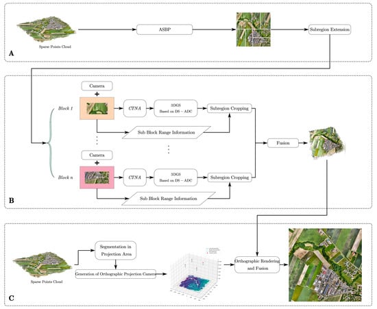
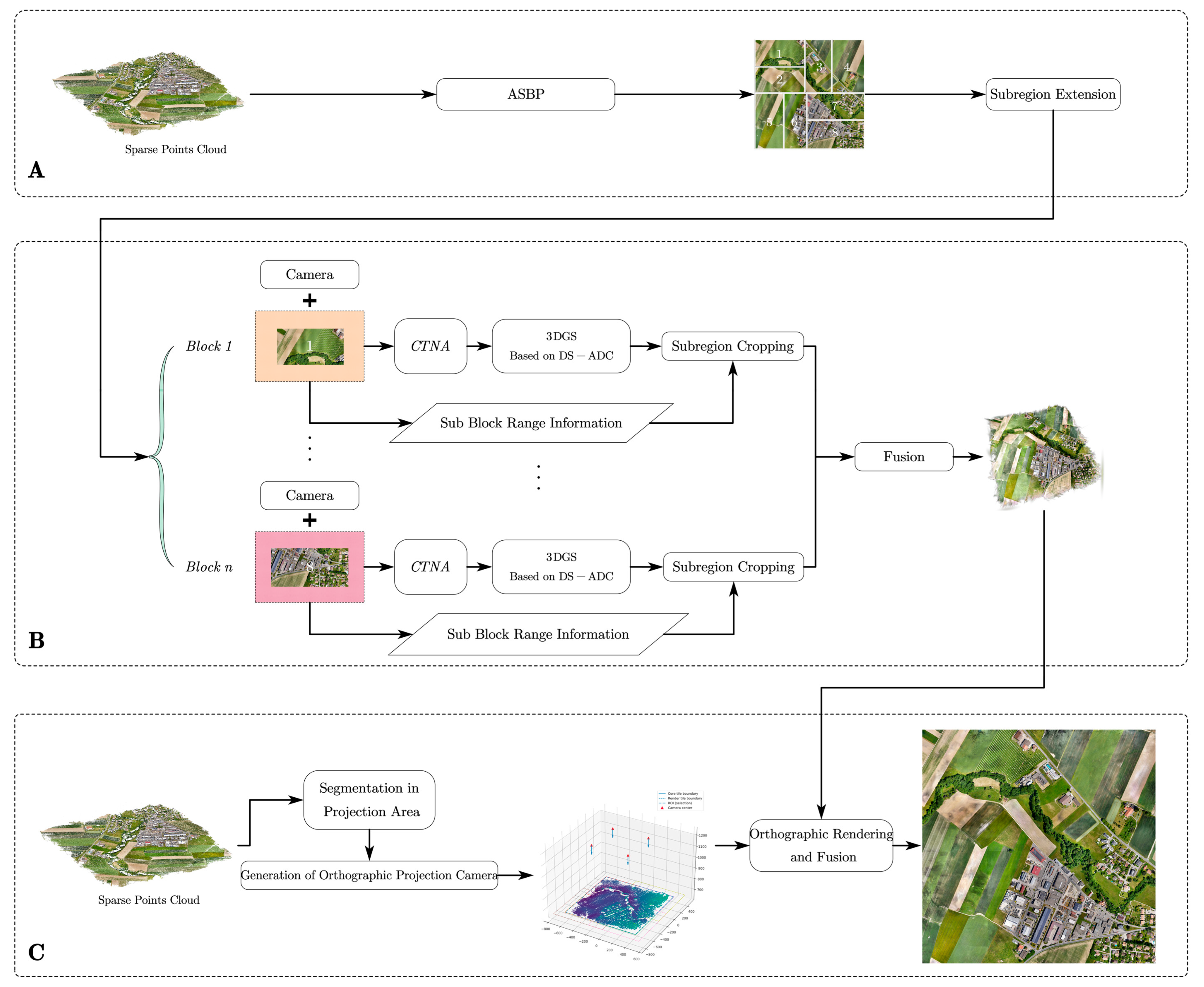
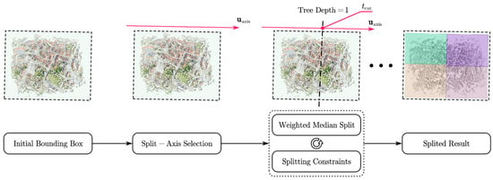
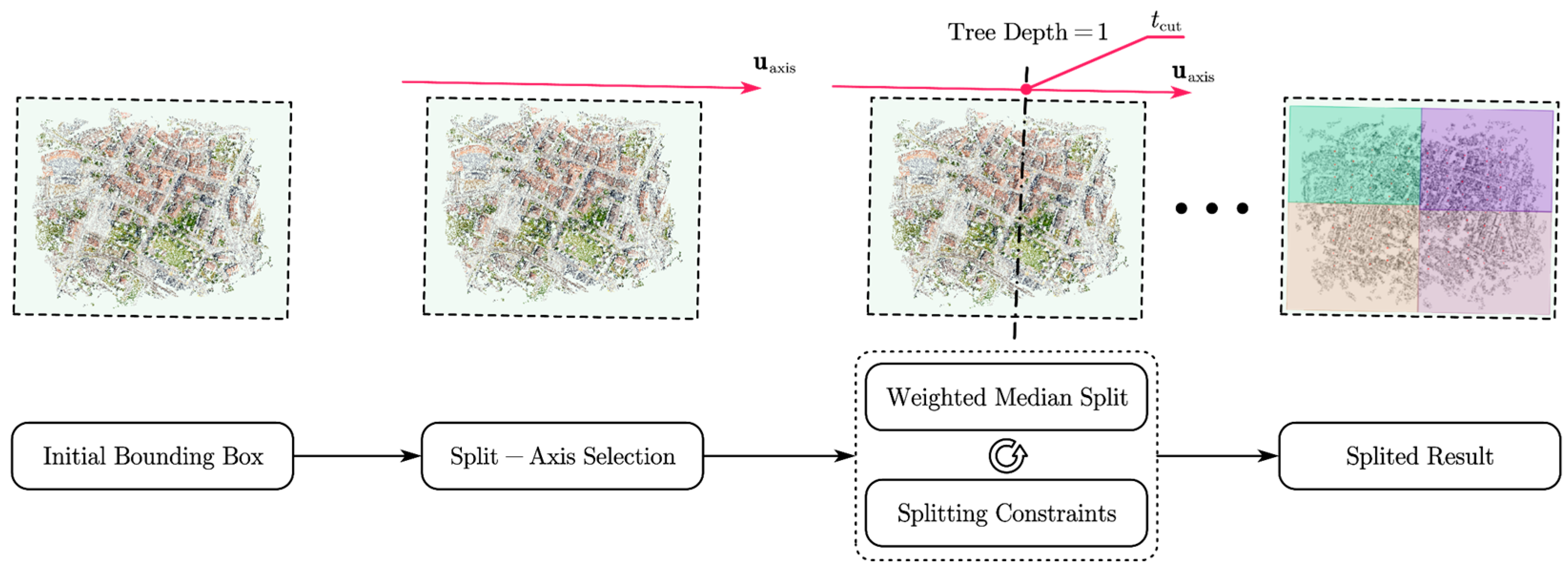
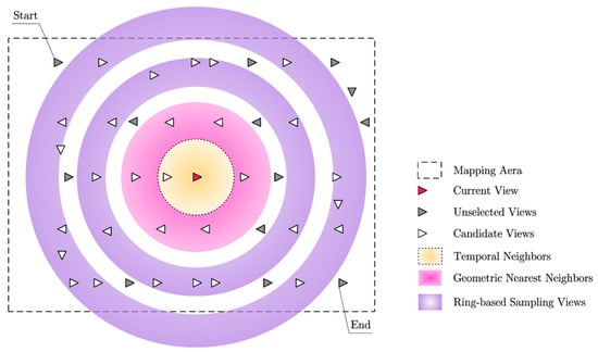
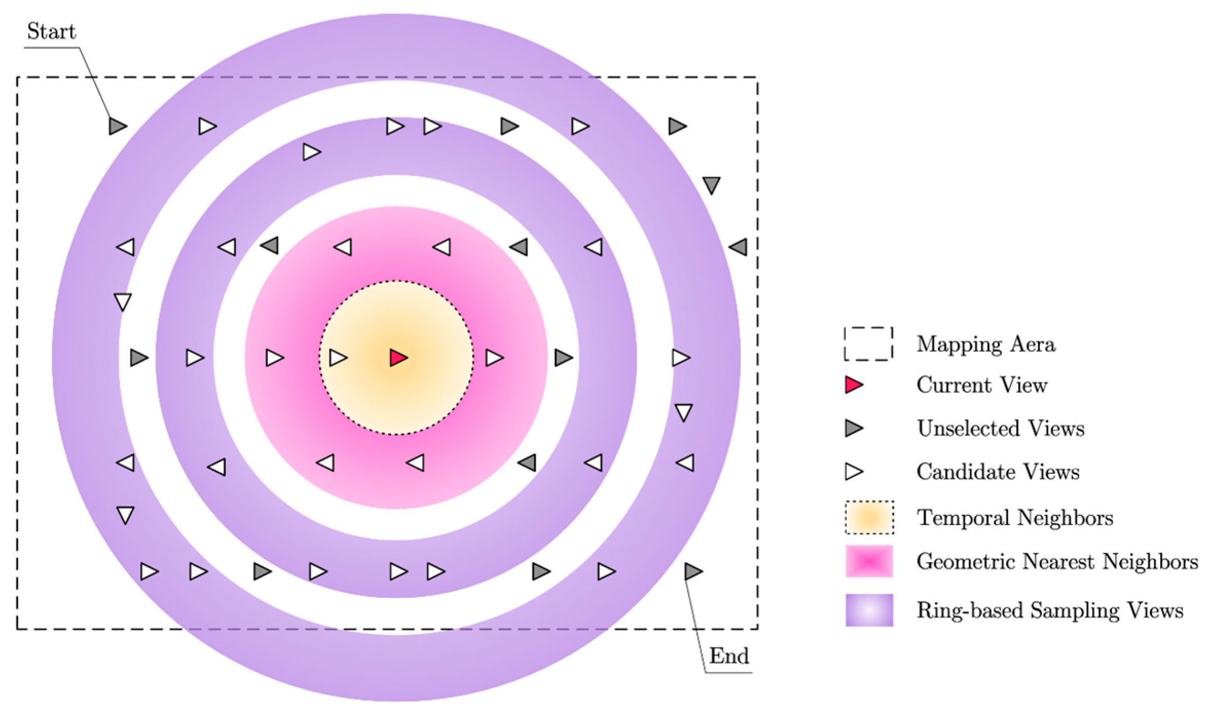
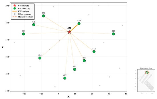
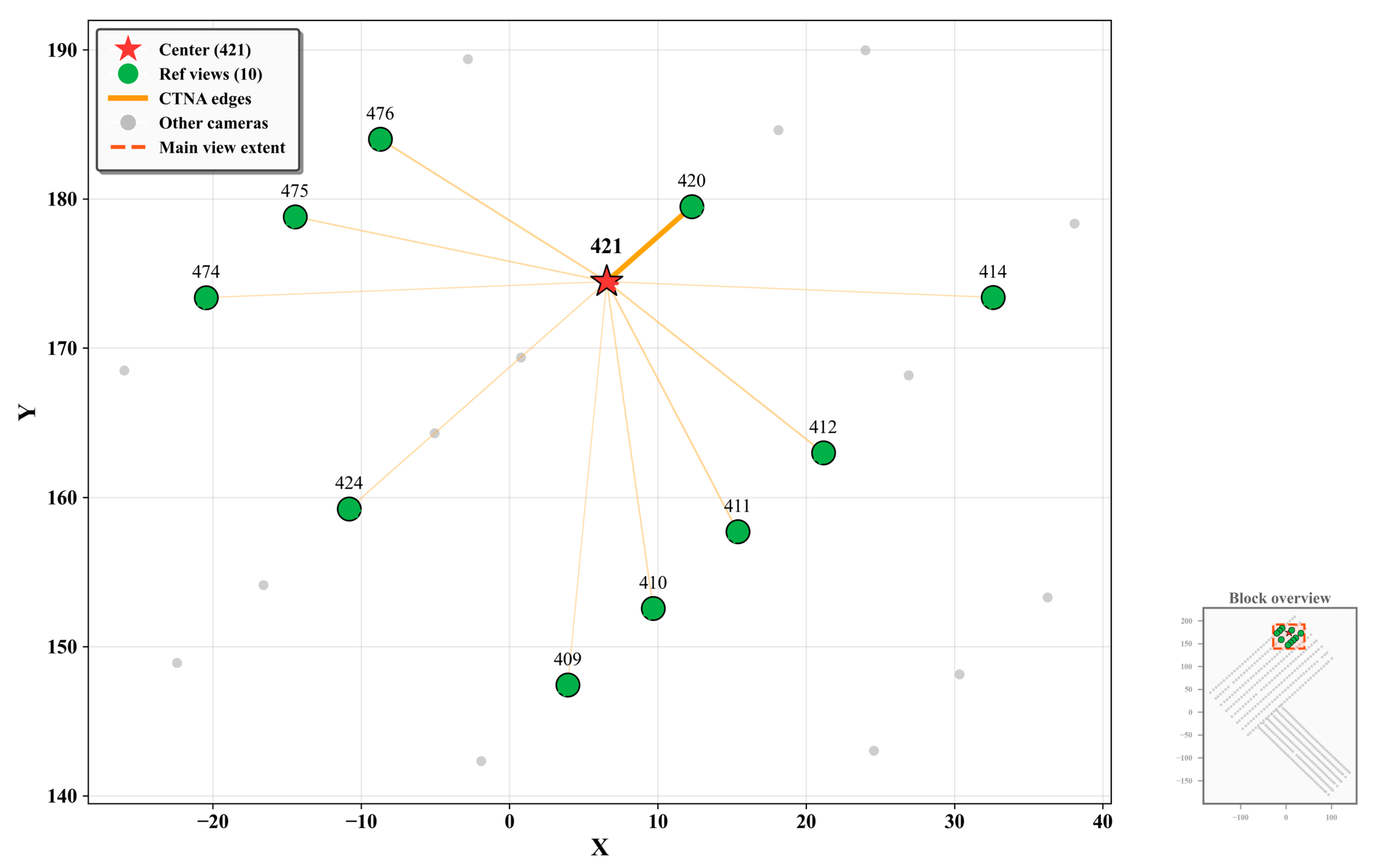
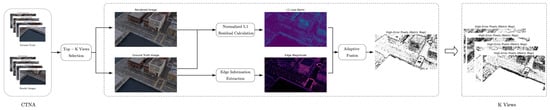

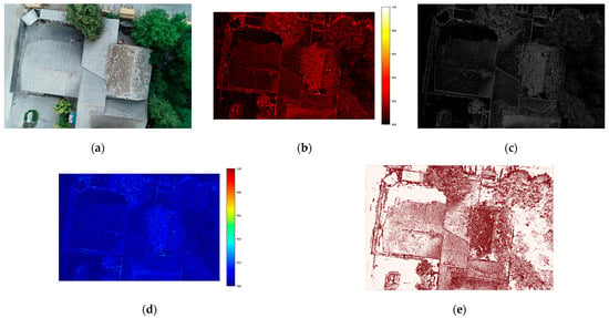
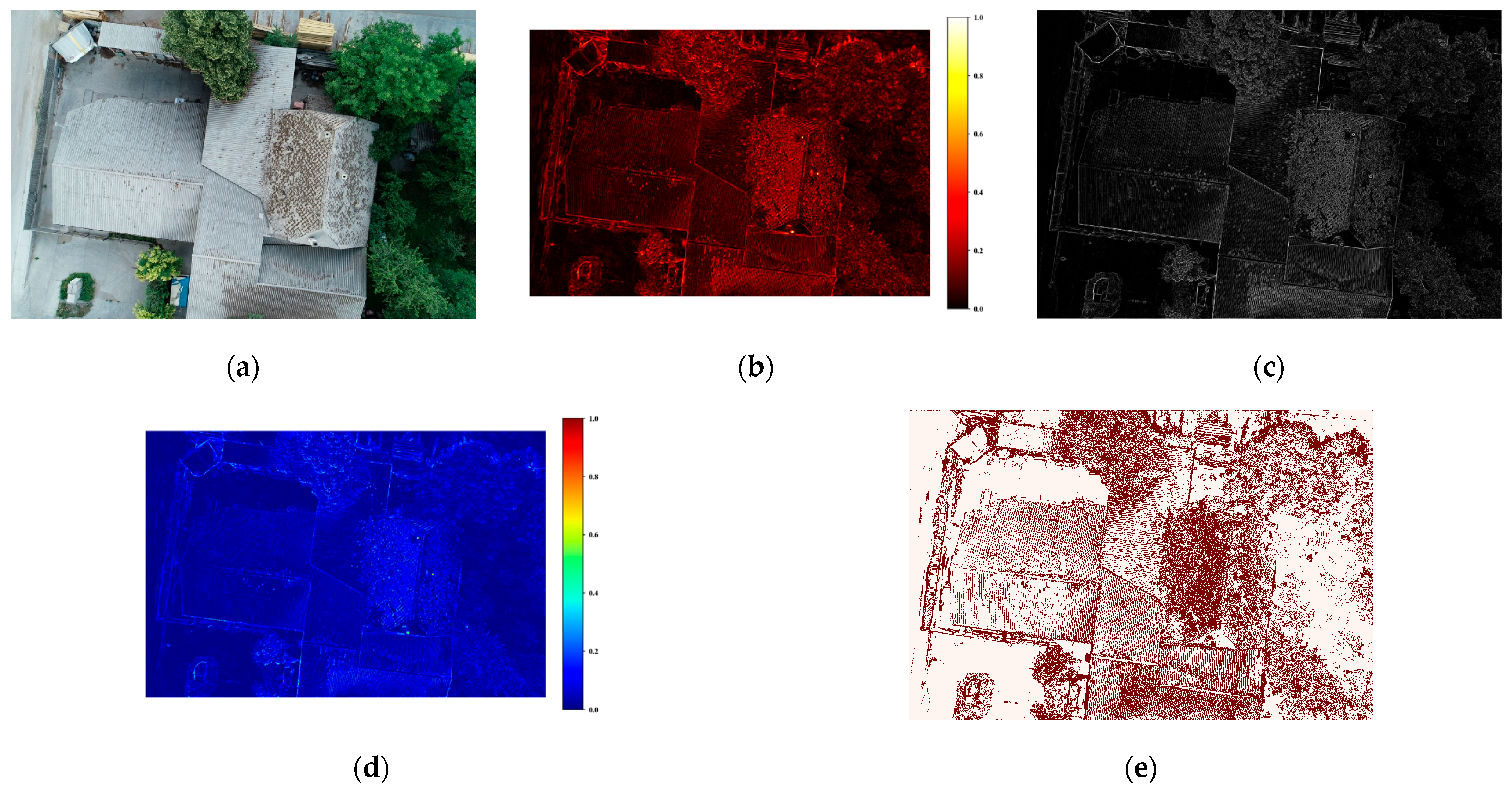
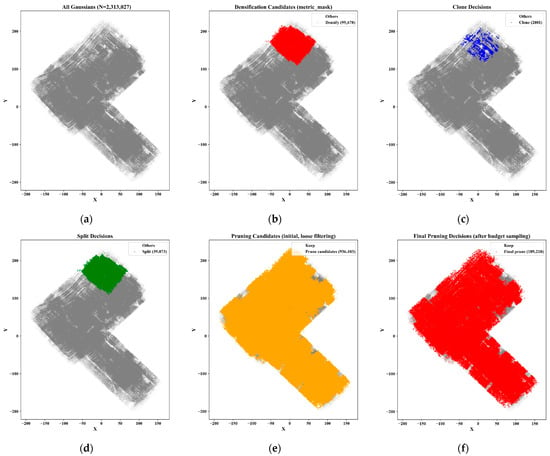
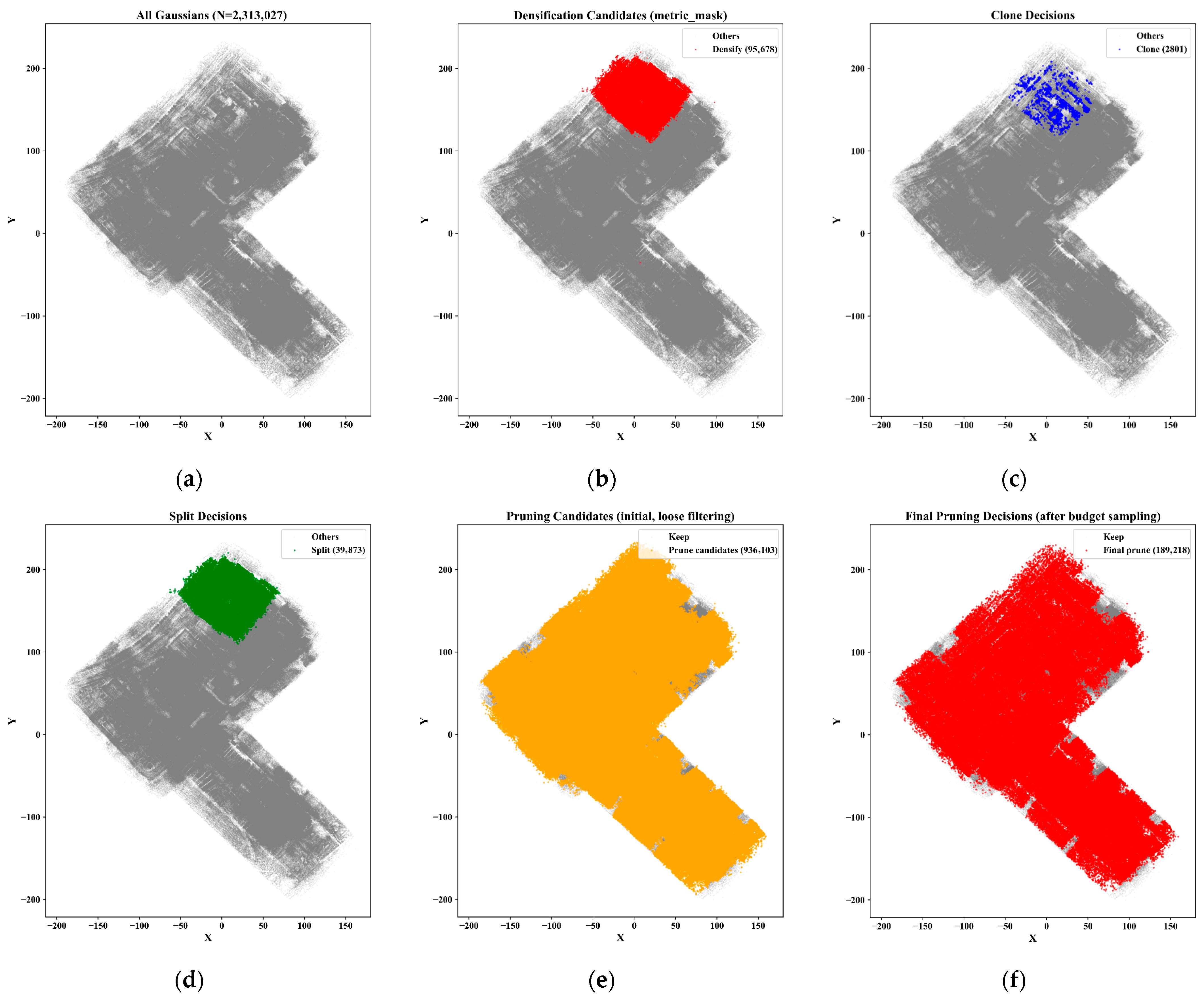
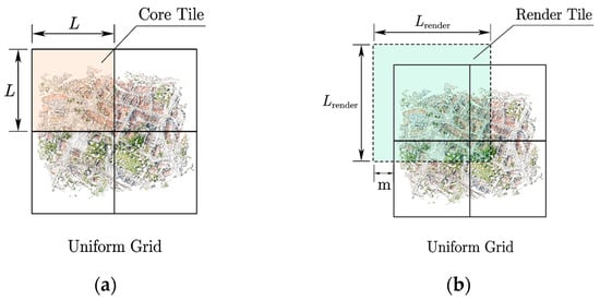
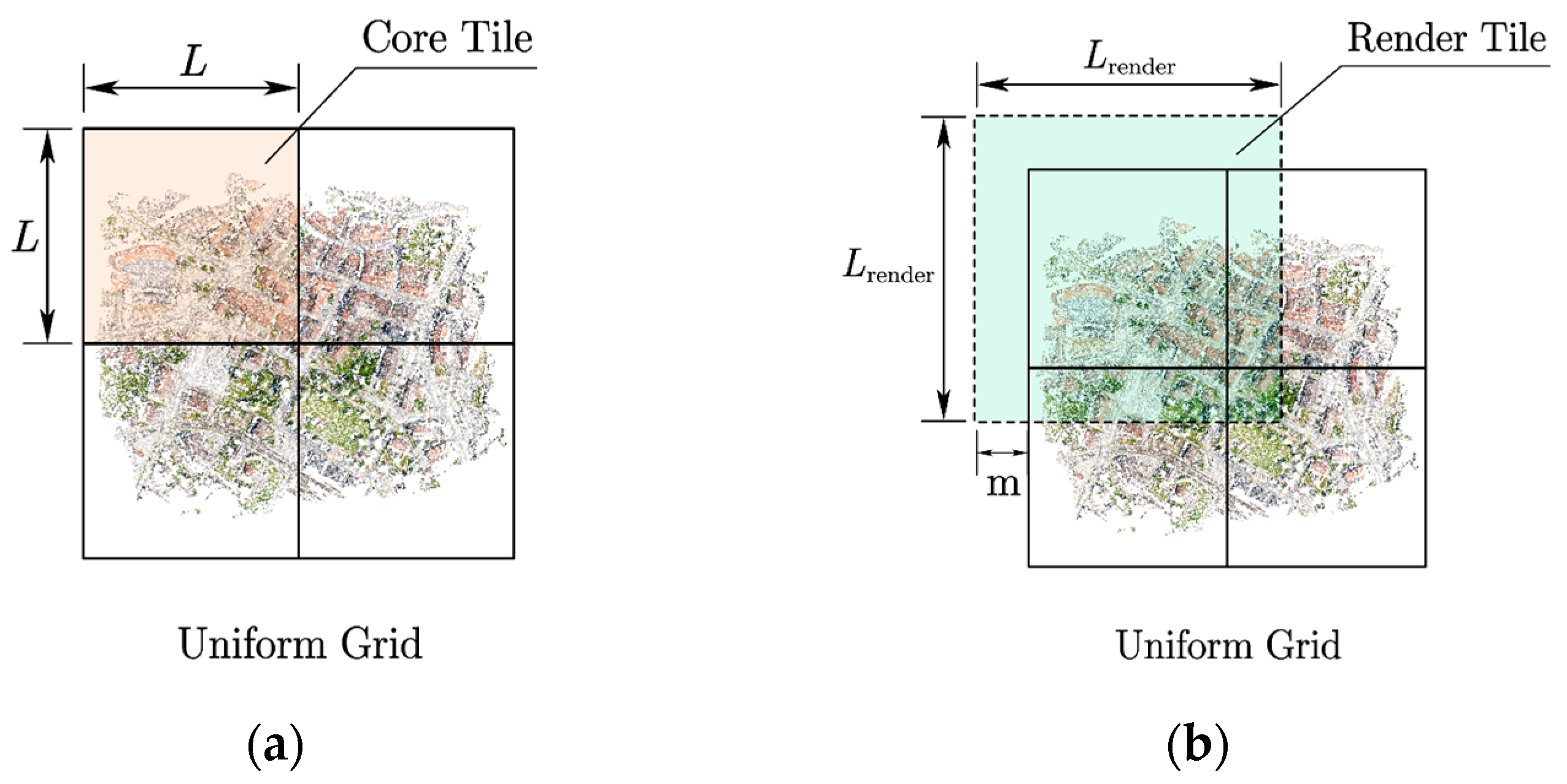
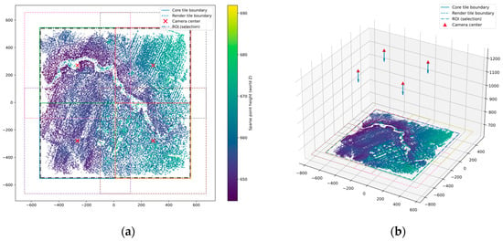
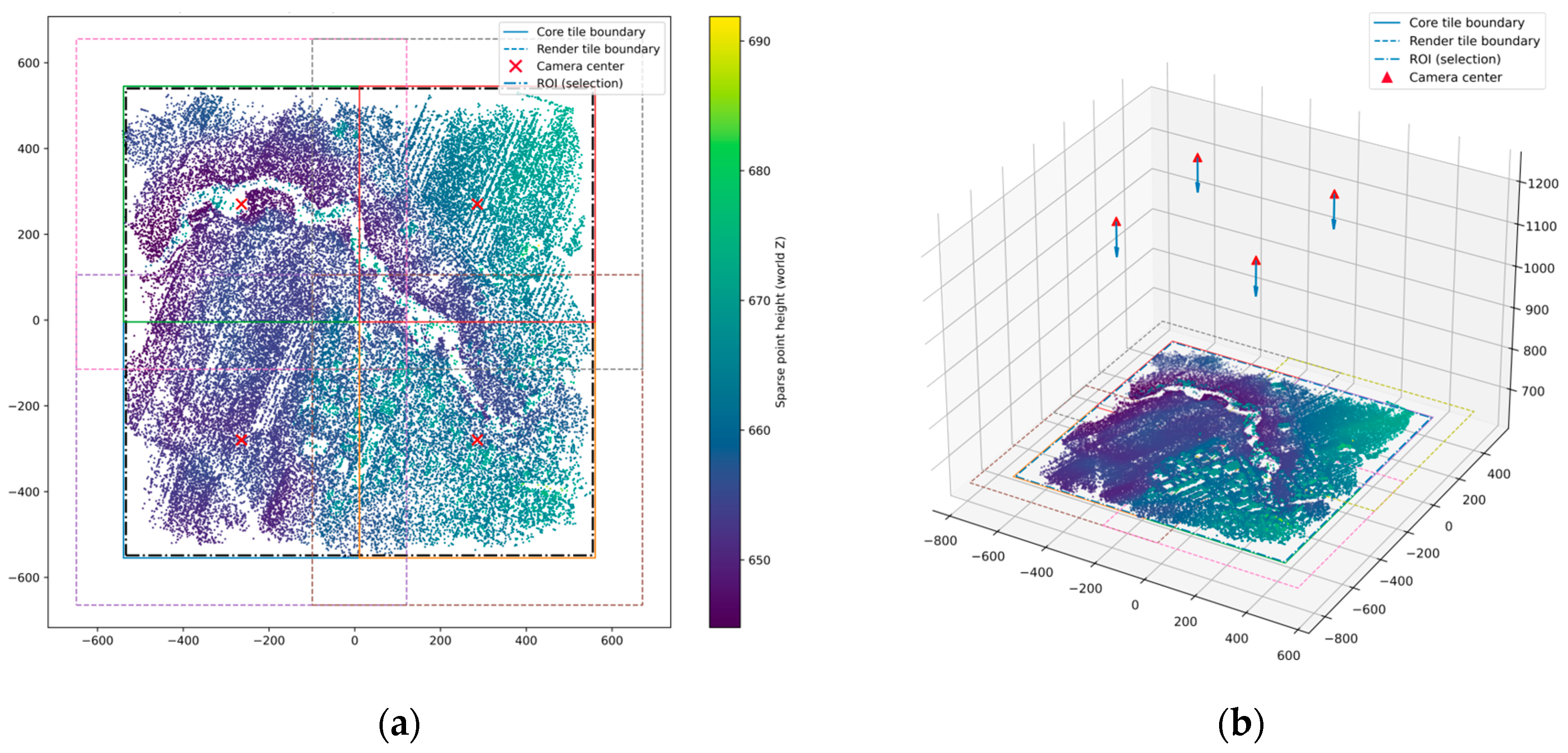
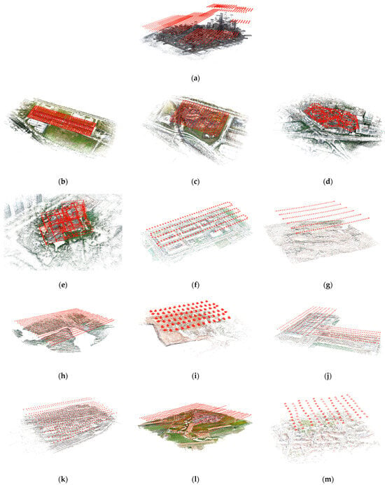
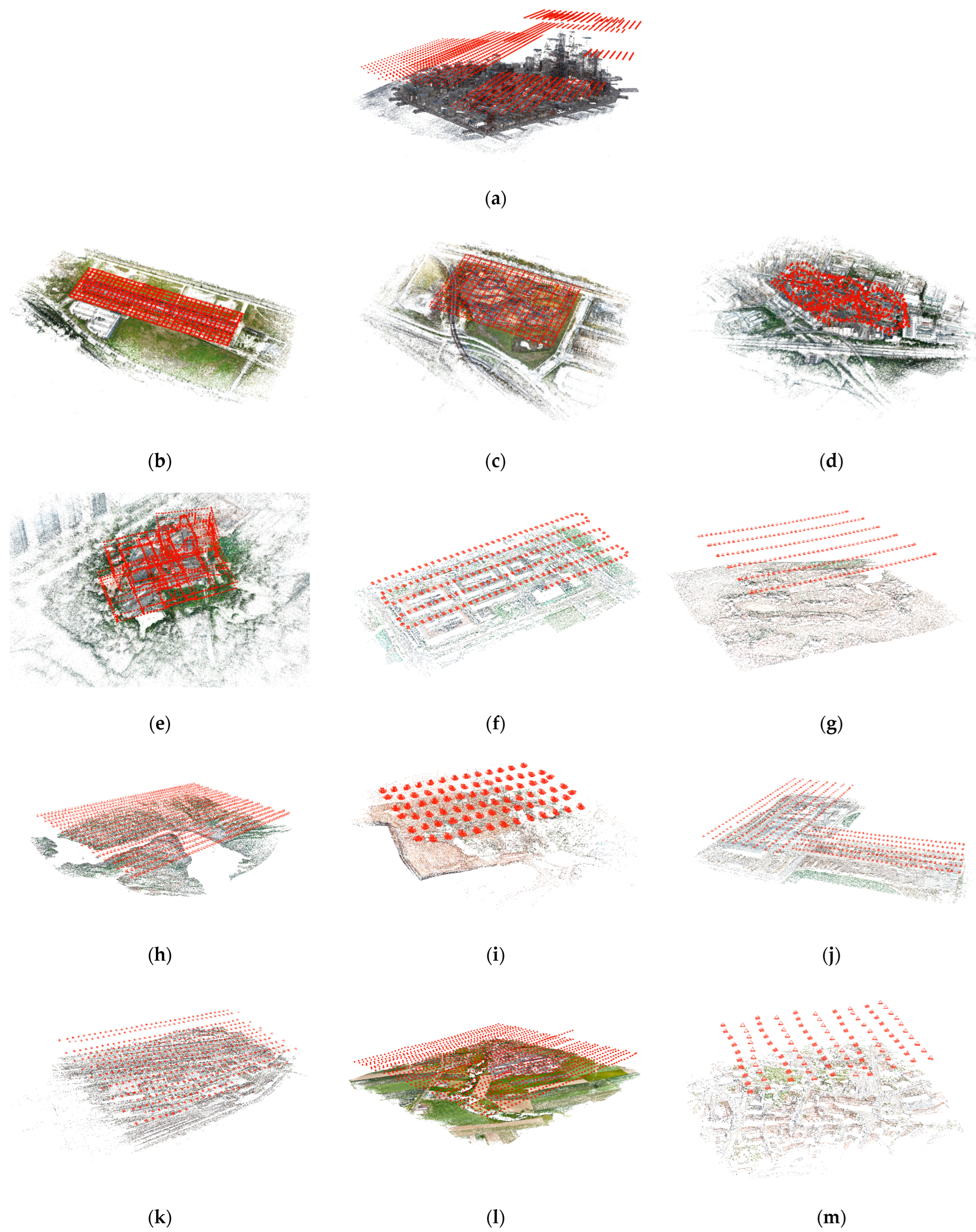
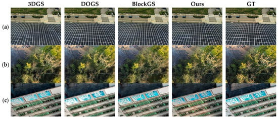
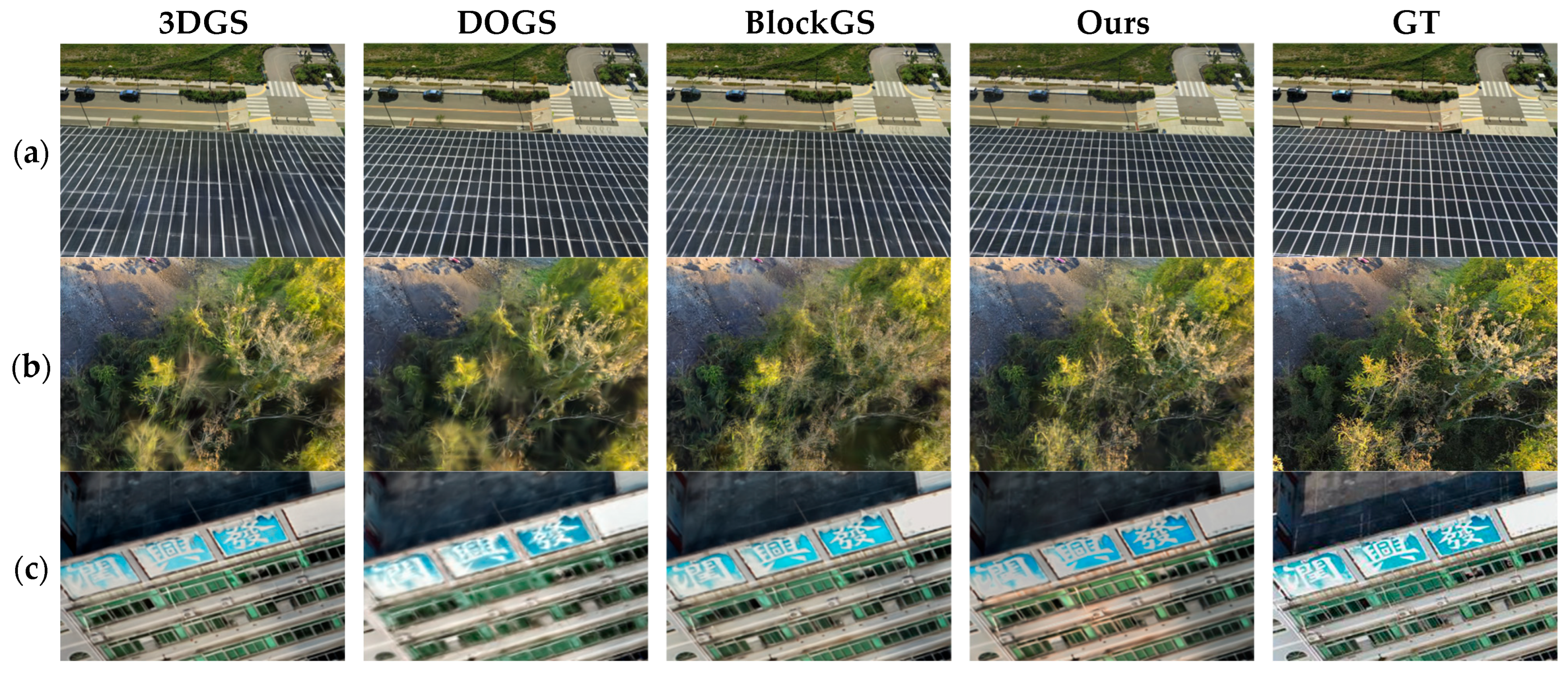
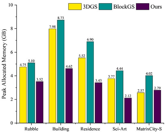
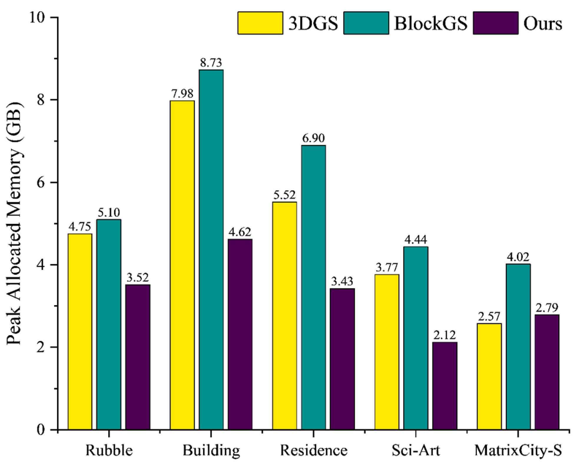
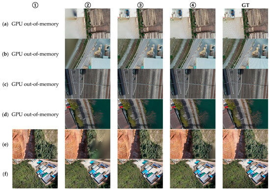
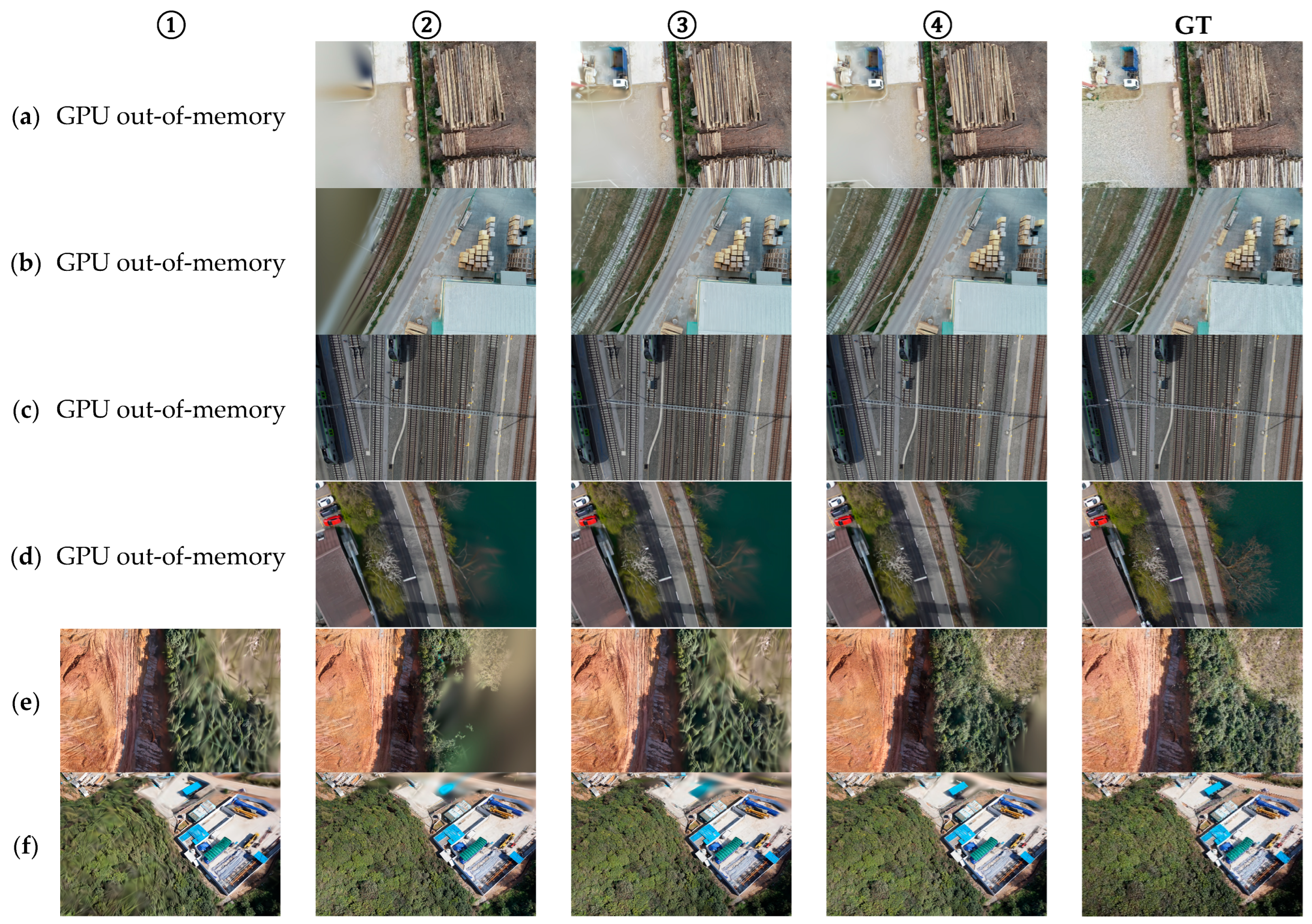
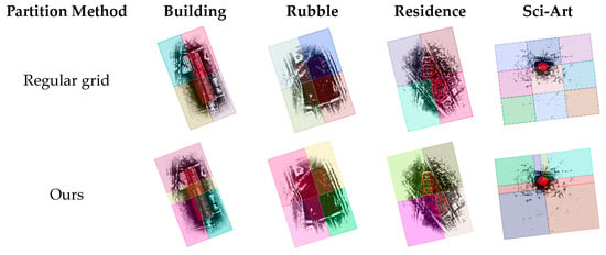
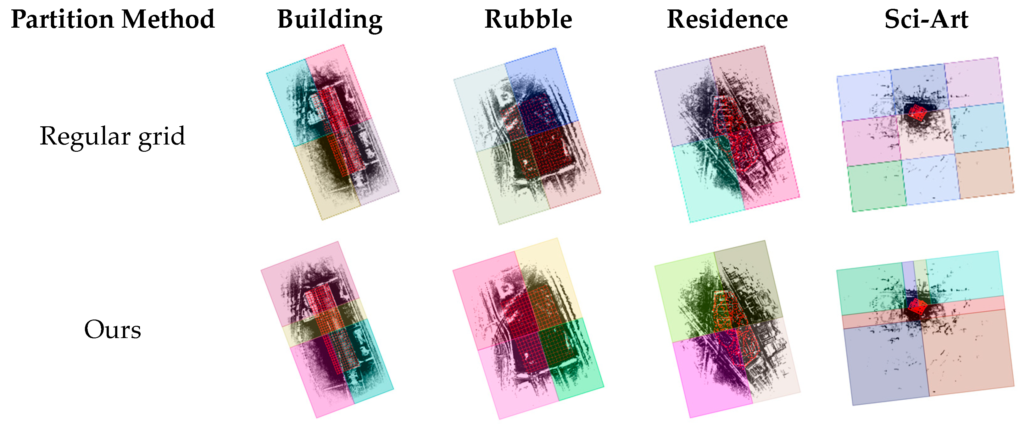
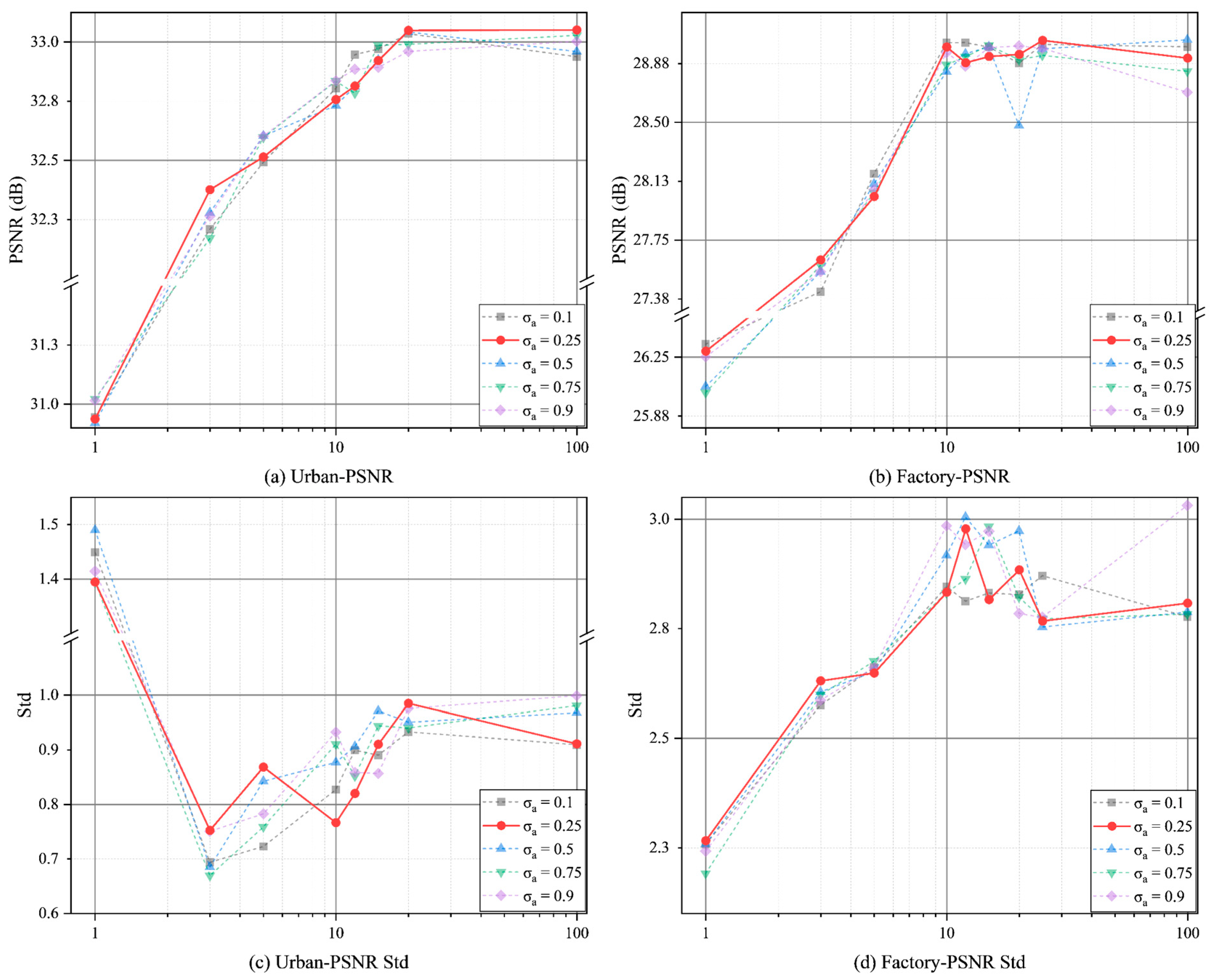
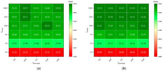
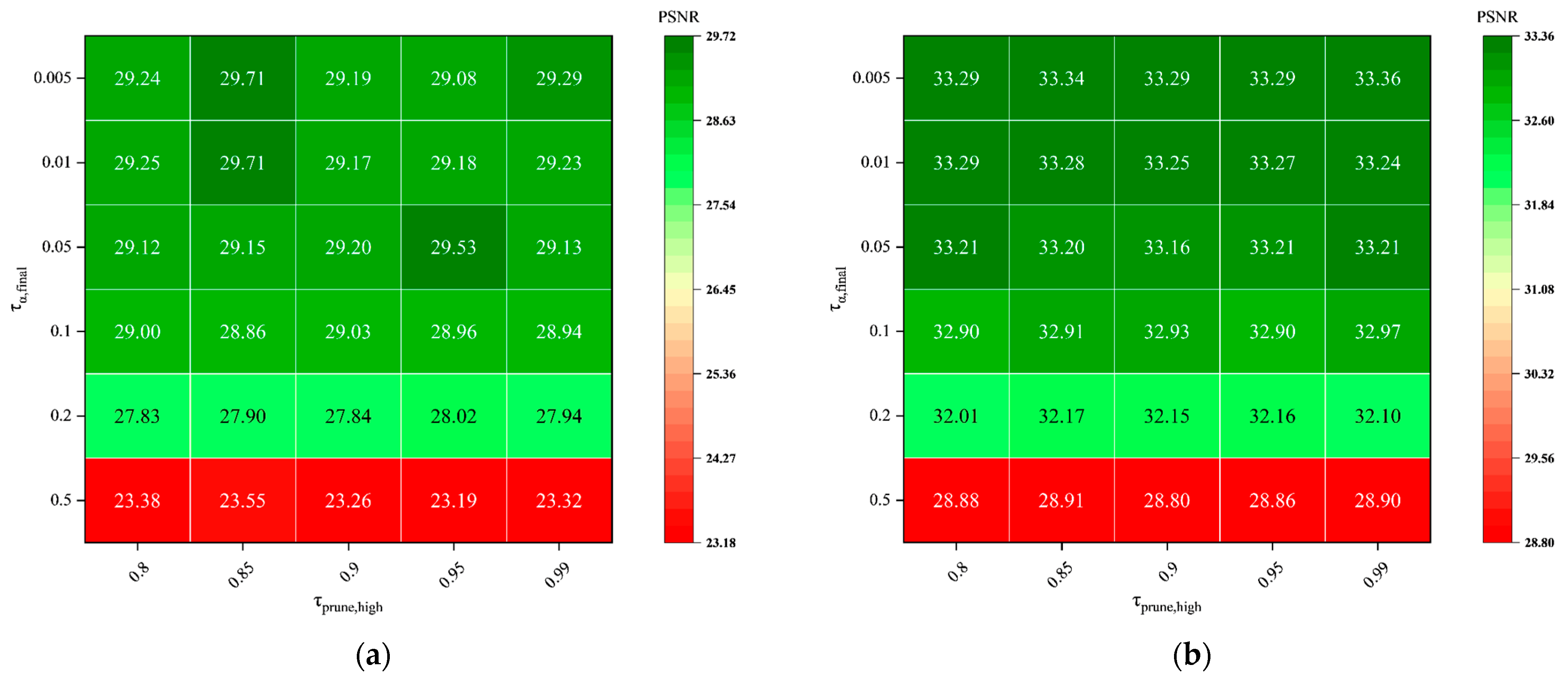
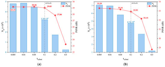
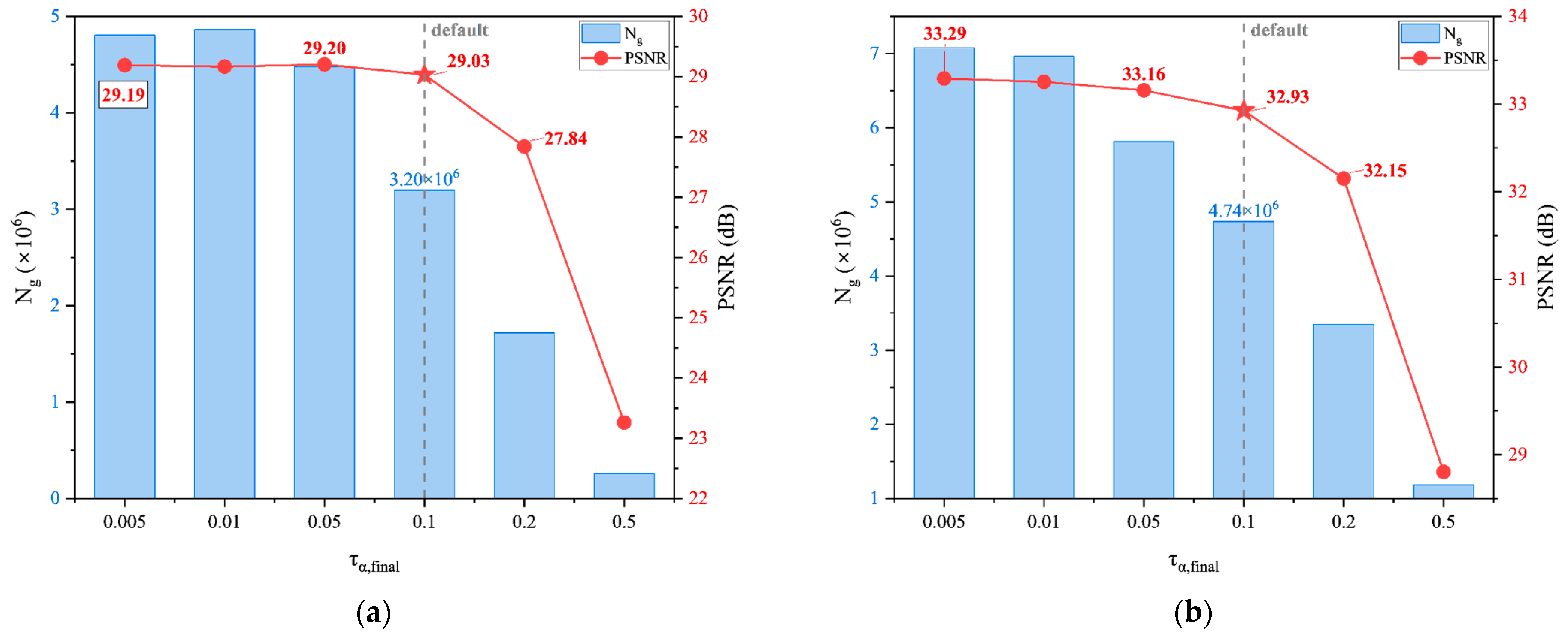
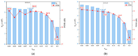
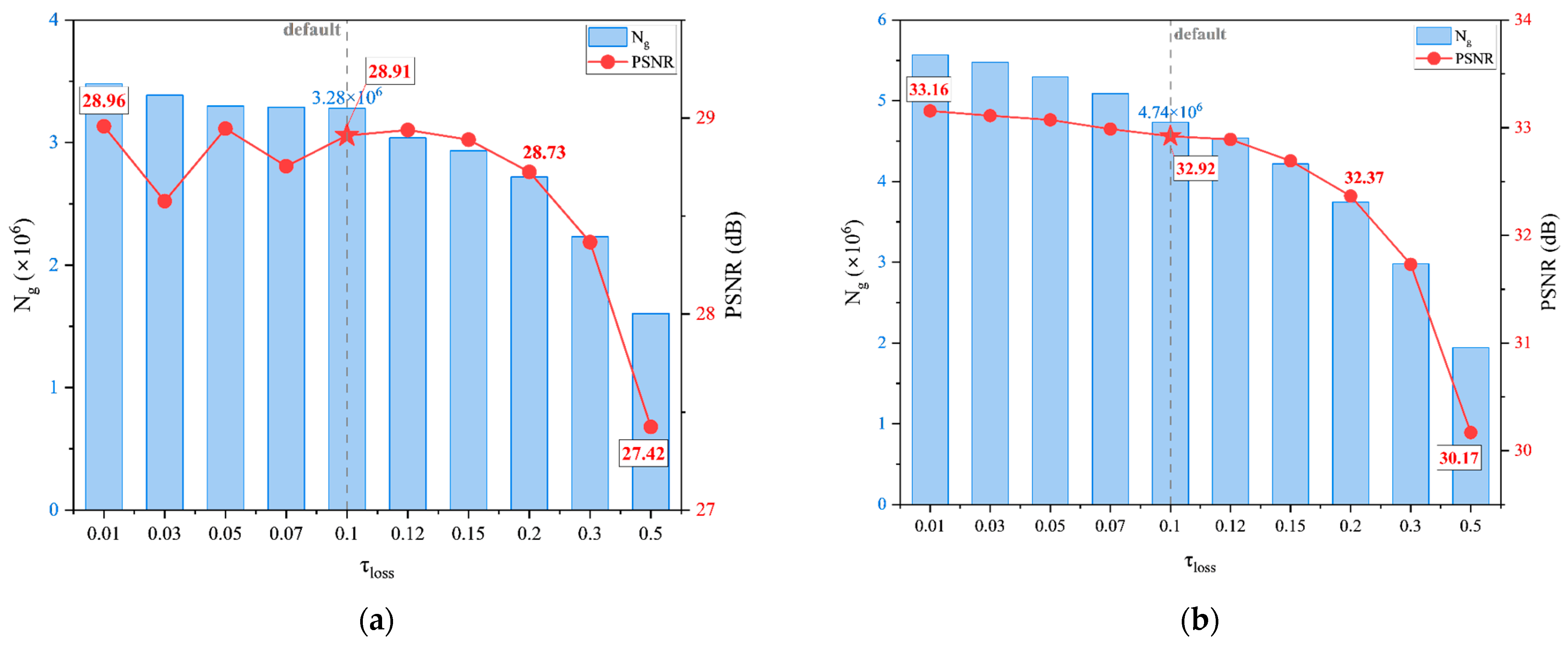
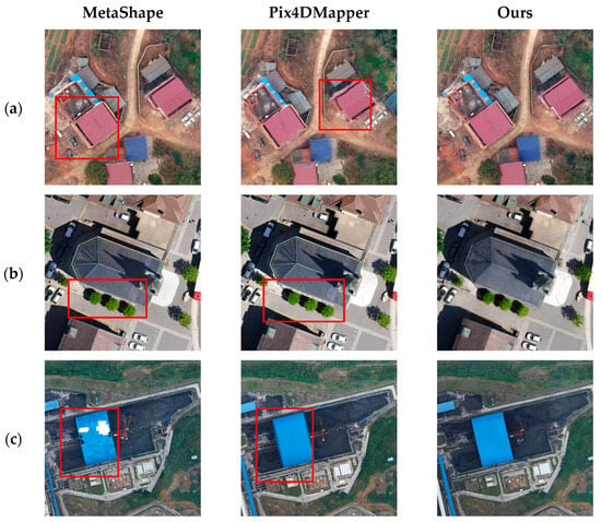
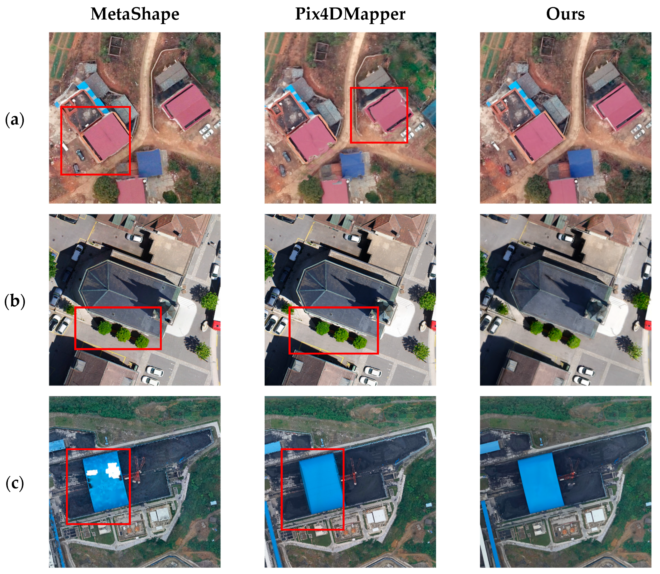
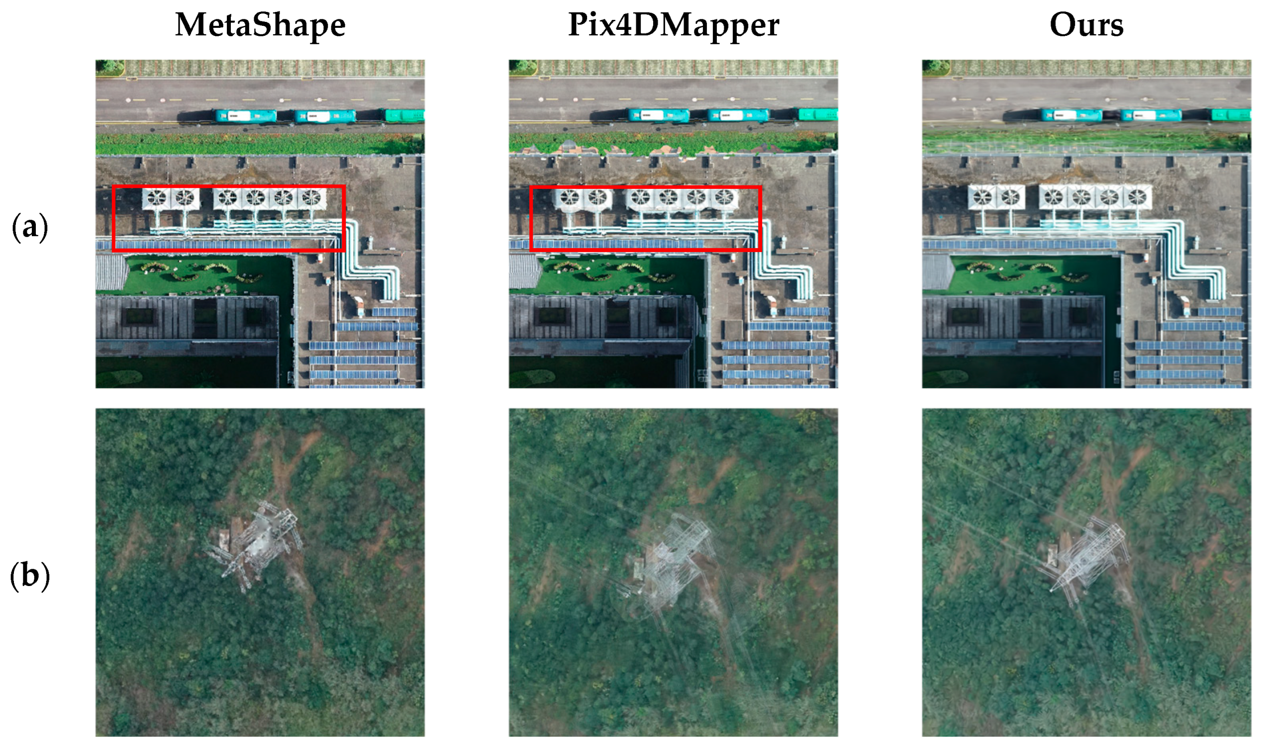
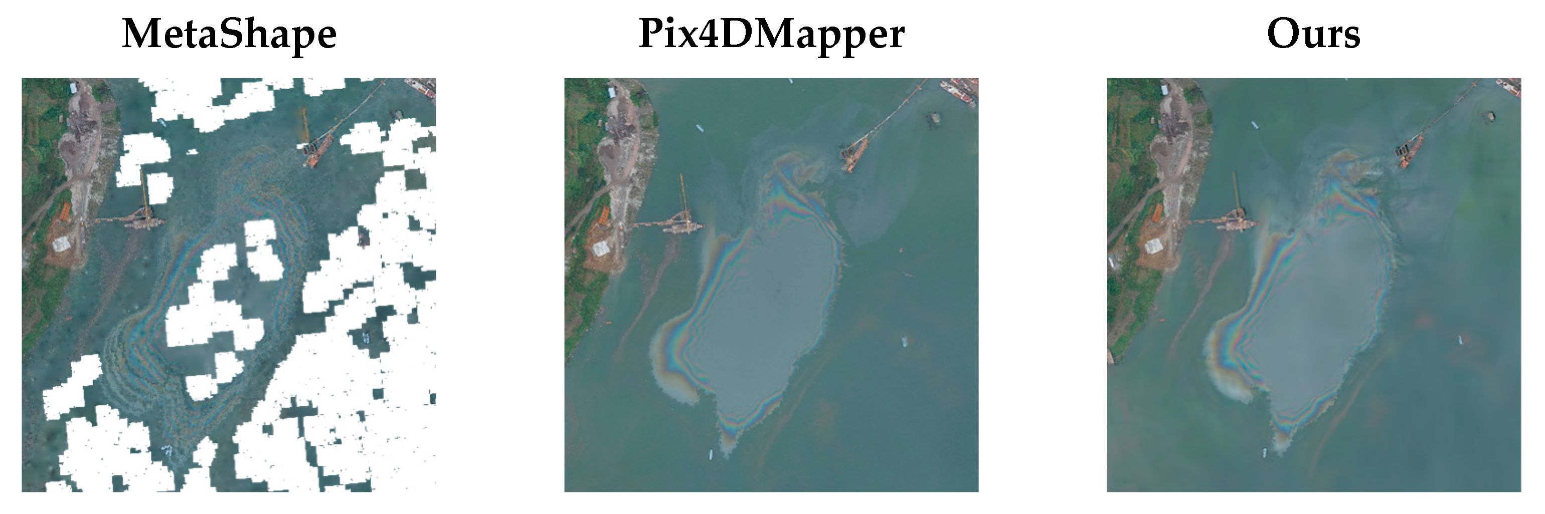
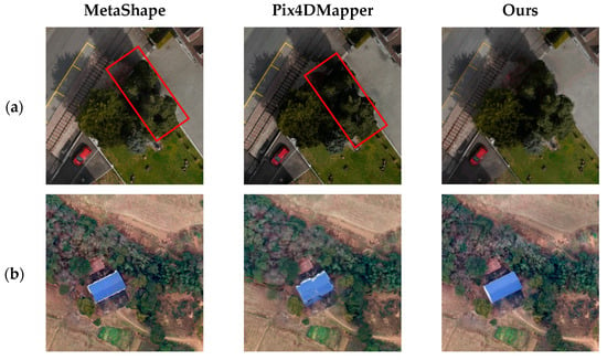
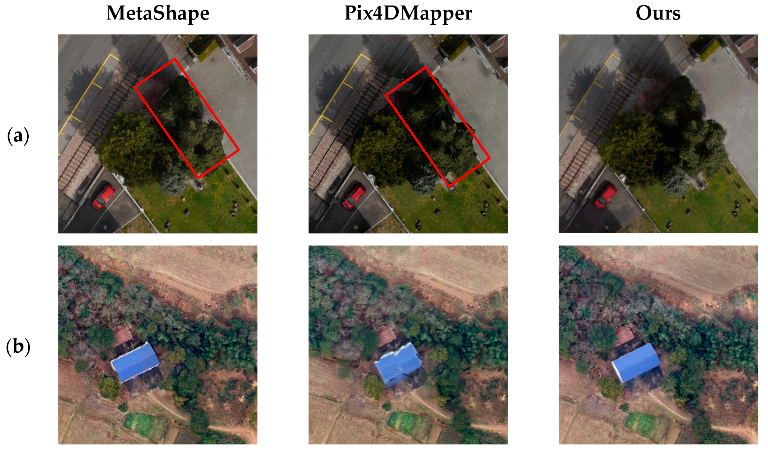
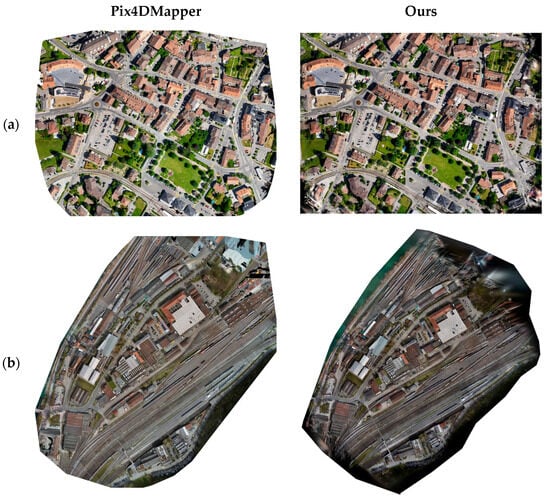
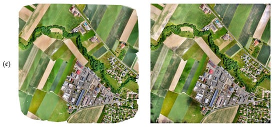
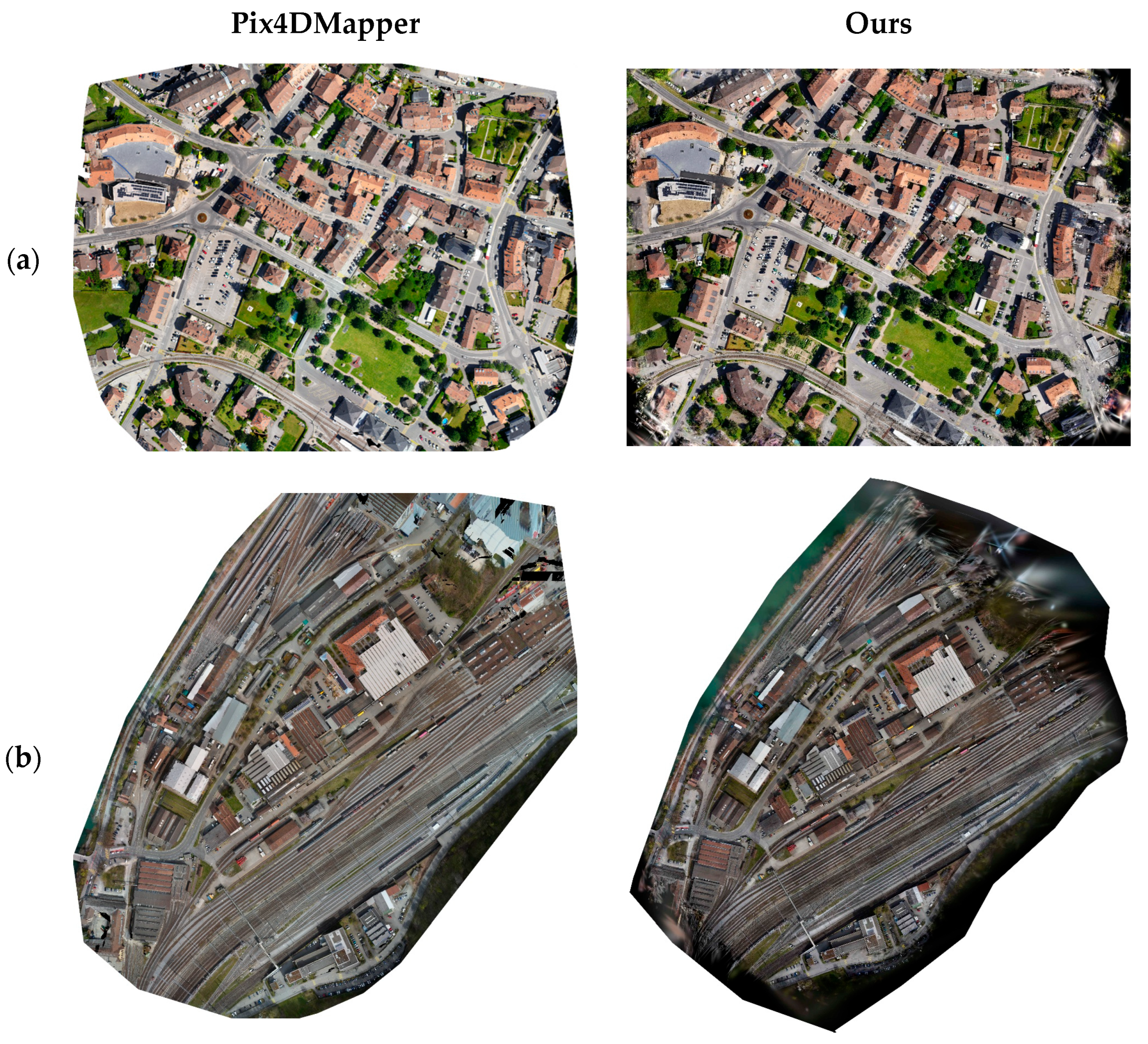
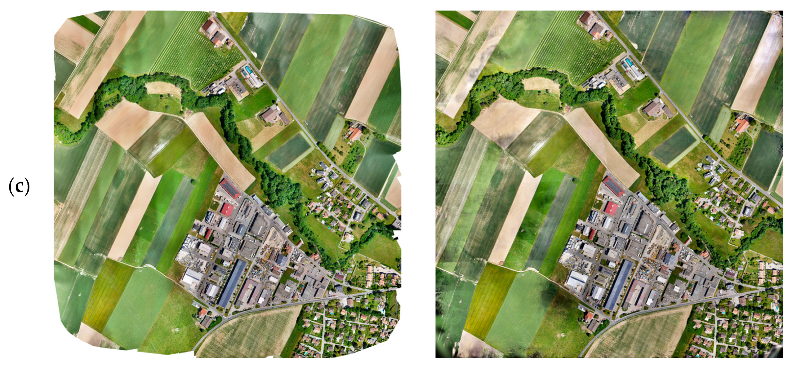
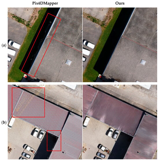
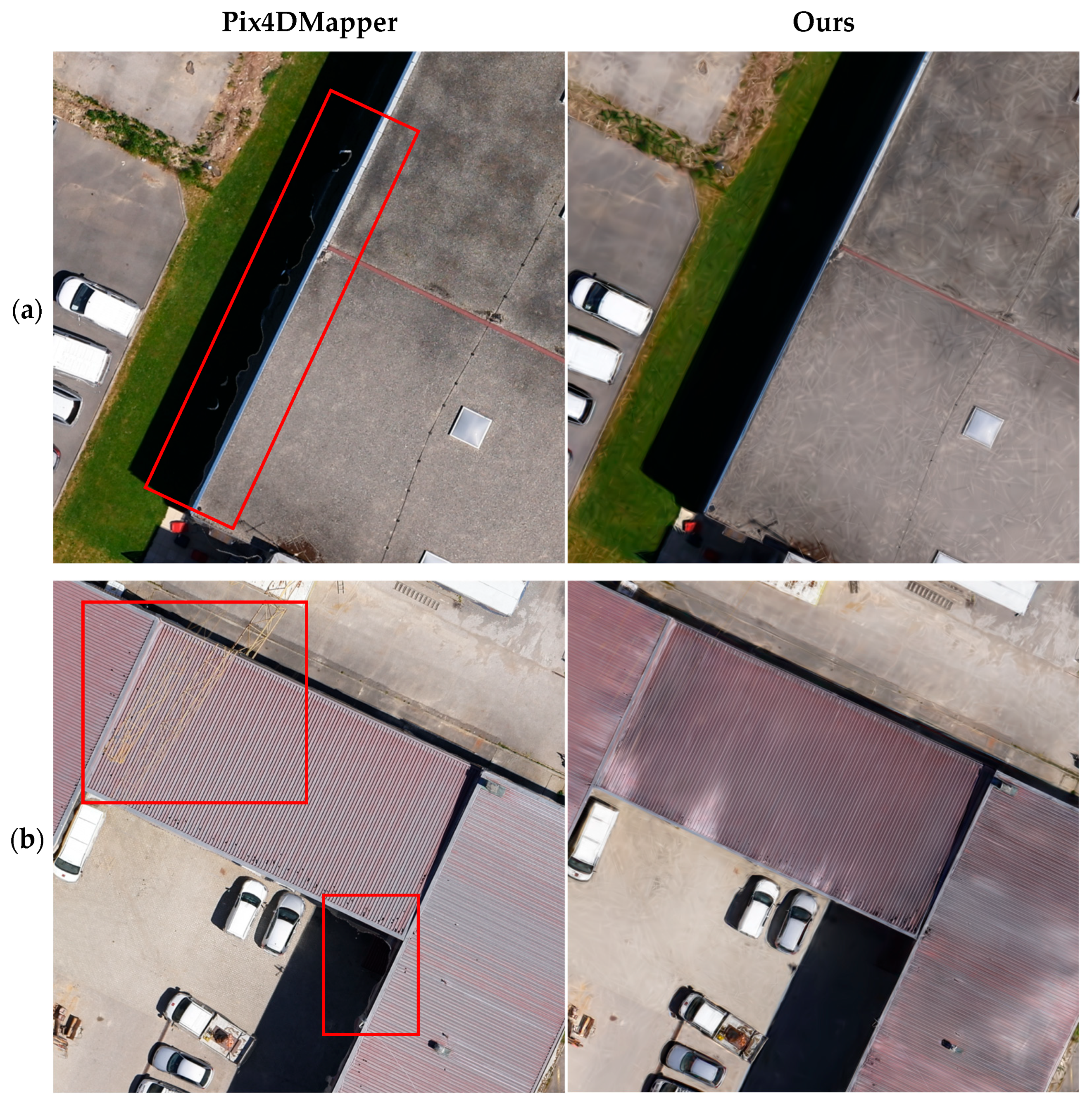

Disclaimer/Publisher’s Note: The statements, opinions and data contained in all publications are solely those of the individual author(s) and contributor(s) and not of MDPI and/or the editor(s). MDPI and/or the editor(s) disclaim responsibility for any injury to people or property resulting from any ideas, methods, instructions or products referred to in the content. |
© 2026 by the authors. Licensee MDPI, Basel, Switzerland. This article is an open access article distributed under the terms and conditions of the Creative Commons Attribution (CC BY) license.