Article

A Sequential Cooperative Inversion Framework of DC Resistivity and Frequency-Domain Electromagnetic Data to Enhance Subsurface Imaging in Geoscience and Engineering

by
Ramin Varfinezhad
1,
Saeed Parnow
2,3,*,
Francois Daniel Fourie
4 and
Fabio Tosti
2,3
1
Institute of Geophysics, University of Tehran, Tehran 1435944411, Iran
2
School of Computing and Engineering, University of West London, London W5 5RF, UK
3
The Faringdon Research Centre for Non-Destructive Testing and Remote Sensing, University of West London, London W5 5RF, UK
4
The Institute for Groundwater Studies, University of the Free State, Bloemfontein 9300, South Africa
*
Author to whom correspondence should be addressed.
Remote Sens. 2026, 18(9), 1404; https://doi.org/10.3390/rs18091404
Submission received: 25 February 2026 / Revised: 25 April 2026 / Accepted: 27 April 2026 / Published: 1 May 2026

Highlights

What are the main findings?
  • Synthetic modelling indicates that individual inversions of DC resistivity and FDEM data have limitations in resolving the geometry of complex, compact, and dyke-like sources.
  • The sequential cooperative inversion strategy leads to more consistent imaging results, successfully integrating the complementary strengths of both geophysical methods.
  • Results from the Morgenzon Farm site in South Africa demonstrate that DC resistivity models constrained by FDEM data provide improved reconstruction of dolerite dykes.
What are the implications of the main findings?
  • The sequential cooperative approach effectively reduces structural ambiguity, achieving higher fidelity in subsurface geometry and amplitude compared to separate inversions.
  • The proposed algorithm is computationally efficient, converging to a consistent model in fewer than 10 iterations.
  • This approach establishes a robust non-destructive testing (NDT) methodology, facilitating more reliable decision-making for geotechnical site investigations and groundwater exploration.

Abstract

The characterisation of subsurface electrical resistivity is a fundamental requirement for geoscientific and engineering applications, including groundwater exploration and structural assessments. This study examines the sequential cooperative inversion of direct current resistivity and frequency-domain electromagnetic data and compares the results to the inverse models obtained from separate (individual) inversions of the datasets. The proposed cooperative framework is applied to both synthetic datasets generated through forward modelling and field data acquired at the Morgenzon Farm site, South Africa, to delineate a dolerite dyke of hydrogeological significance. Individual inversions identified distinct features but exhibit limitations: direct current resistivity highlights a two-layered medium with minor anomalies, while frequency-domain electromagnetic data identify a resistive anomaly. In contrast, the sequential cooperative inversion approach, which uses the output of one dataset to constrain the other, provides improved subsurface imaging results, reduces ambiguity, and enables the integration of complementary information from both methods. The results indicate that resistivity models constrained by inverse frequency-domain electromagnetic data provide improved representation of subsurface geometry and amplitude compared to individual approaches. These findings support the use of a non-destructive testing approach for improved subsurface imaging, facilitating better-informed decision-making in infrastructure projects and resource management.

1. Introduction

Obtaining models of the subsurface that can be interpreted in terms of their geological causes is an important stage in engineering geophysics. This process is highly dependent on recovery algorithms such as inversion techniques, which are essential for geotechnical site characterisation and infrastructure monitoring. Conventional inversion of geophysical datasets, such as DC resistivity and FDEM data, provides valuable insights into the subsurface structure but often faces challenges of non-uniqueness and instability in their inverse solutions [1]. These challenges arise because geophysical inversion problems are inherently ill-posed, affected by noise, and limited by the individual methods’ ability to resolve complex features.
In the context of civil and environmental engineering, reducing the uncertainty of these models is important for supporting risk-informed decision-making during construction and resource management. Integrating multiple geophysical datasets during inversion has emerged as a promising strategy to address these challenges [2]. By combining complementary datasets, DC resistivity with gravity, electromagnetic, and seismic data [3,4,5], the strengths of each method can be leveraged to reduce ambiguity and improve the reliability of subsurface characterization.
Geophysical datasets can be integrated through several approaches. One common method is joint interpretation, where each dataset is first inverted separately, and the resulting models are then interpreted together using geological and other supporting information [6,7,8,9,10].
Another approach is joint inversion, which combines multiple datasets within a single framework using petrophysical or structural constraints [11,12], or by enforcing structural similarities between models [6,12,13]. More recently, artificial intelligence (AI) algorithms have been developed to facilitate this integration [14], improving the resolution and accuracy of subsurface imaging.
A further integration strategy, and the focus of this study, is cooperative inversion, in which the inversion result of one geophysical method serves as a constraint model or reference model for another [1,15]. Different definitions for cooperative inversion exist across scientific literature. For instance, within the broader geophysical community, Lines et al. [16] defined cooperative inversion as the estimation of an underground model consistent with various independent geophysical datasets. According to this definition, cooperative inversion may include either joint inversion or sequential inversion, where the latter is most frequent. On the other hand, in some studies, cooperative inversion refers specifically to a simultaneous joint inversion, in which multiple datasets are inverted together to recover a single shared physical property model. For example, Mohand-Said et al. [17] performed a cooperative joint inversion of time-domain electromagnetic and direct current resistivity data by simultaneously minimising a combined objective function to recover a common resistivity model. In this case, the cooperation occurs through the simultaneous fitting of both datasets within a single inversion framework.
In this study, sequential cooperative inversion (Figure 1) is presented as a robust NDT strategy for improving subsurface imaging. This approach involves using the inversion results of one geophysical dataset as an initial model for the inversion of the other dataset. The role of the initial model is important in local optimisation-based inversions (e.g., Gauss–Newton, conjugate gradient methods), where poor starting models may lead to convergence issues or local minima (e.g., [2,18]). For engineering applications, stable convergence is important for obtaining consistent and interpretable subsurface models [19,20].
This study introduces a sequential cooperative inversion approach for the integration of DC and FDEM techniques, a combination that has not been previously explored. The DC resistivity and FDEM methods are inherently linked through their respective association with resistivity ( ρ ) and conductivity ( σ ), where ρ = 1 / σ . This direct physical relationship allows for a more streamlined and engineered inversion workflow compared to methods relying on unrelated physical parameters.
While the joint interpretation of these data has been documented [21,22], to our knowledge, no prior studies have investigated their sequential cooperative inversion to enhance imaging fidelity. This gap motivates the present study, which evaluates the capability of sequential information transfer between DC resistivity and FDEM datasets. A conceptual analogy may be drawn with broader geophysical modelling approaches, where prior physical constraints are incorporated to guide inversion processes. For example, Quinn et al. [23] described a global-scale application in which electrical conductivity constraints were used to inform geomagnetic data inversion. Although the scale and application differ, this illustrates the general principle of constraint-driven inversion. We investigate the efficacy of cooperative inversion of DC resistivity and FDEM data in obtaining reliable models of the subsurface structure. We first present the individual inversions for each dataset, which are based on linear integral equations [21,24,25]. Following this, we introduce the cooperative inversion framework and evaluate its performance through applications to both synthetic datasets and field data collected across a dolerite dyke on the Morgenzon Farm site in South Africa, a key indicator of groundwater presence in the study area. The cooperative inversion results are compared with the individual inversions to evaluate the success of cooperative inversion in obtaining improved models of the subsurface for geoscience and engineering applications.

1.1. Literature Review: Multi-Modal Geophysics and Integrated Frameworks

The growing need for high-resolution subsurface imaging across geoscience and engineering disciplines has accelerated the development of integrated geophysical approaches. Although individual geophysical datasets offer valuable baseline information, their inverse solutions often suffer from non-uniqueness and instability, limiting their effectiveness for engineering-grade structural assessment. To overcome these limitations, recent research emphasises integrated and multi-method approaches as an essential means of reducing uncertainty and lowering technical risk in complex subsurface investigations.

1.2. Case Studies in Cooperative and Joint Inversion

Historically, the integration of diverse geophysical datasets has been widely explored across various engineering, environmental and exploration sectors. Pasion et al. [26] used cooperative inversion of magnetometry and time-domain electromagnetic data for high-precision detection of unexploded ordnance projects. Similarly, Lelièvre et al. [27] implemented cooperative inversion of seismic and gravity datasets for mineral exploration, while Gonçalves and Leite [28] integrated seismic reflection and gravity datasets through a cooperative inversion procedure.
For precision site characterisation, Paasche and Tronicke [29] introduced a 2D method based on fuzzy c-means clustering to execute cooperative inversion of different datasets, with promising results. Linder et al. [30] utilised and expanded this zonal cooperative inversion approach for the integration of crosshole P-wave, S-wave, and ground penetrating radar (GPR) datasets to reveal and characterise disparate sedimentary units. In this framework, an individual model including GPR velocity and the velocities of P and S waves is extracted as the zonal cooperative inverse model, delineating the main subsurface zonation while explaining all measured datasets.
This algorithm was further extended by Tronicke and Paasche [31] to integrate S- and P-wave travel time data, showing how supportive a priori information can be incorporated automatically to further constrain the final inverse model.
In challenging rock environments where seismic data quality is significantly decreased, Takam Takougang et al. [32] presented a cooperative joint inversion algorithm incorporating magnetotelluric data; Le et al. [33] solved the non-uniqueness of individual inversion of magnetotelluric data due to remarkable near-surface resistivity variations through cooperative inversion with a seismic reflection approach. High-resolution applications also include the work of McMillan and Oldenburg [34], who integrated airborne time-domain electromagnetic, DC resistivity and controlled source audio frequency magnetotellurics to provide 3D high-resolution conductivity (resistivity) images of the subsurface at the Antonio gold deposit in Peru. Furthermore, Skibbe et al. [35] used structurally coupled cooperative inversion of magnetic resonance sounding and vertical electrical sounding for improved conductivity estimations.
Recent advancements have focused on more sophisticated coupling and structural constraints. Le et al. [36] utilised the textural domain for the cooperative inversion of magnetotelluric and seismic reflection datasets. Mutual information sharing between gravity and DC resistivity methods was performed by Singh, Mishra and Sharma [15] using fuzzy c-means clustering, which requires a priori knowledge of the number of geological units. Kim et al. [37] proposed a cooperative inversion algorithm based on the structure tensor that demonstrated improved performance over conventional cross-gradient constraints in extracting average structural information. Cross-gradient methods can be limited when model components exhibit opposing gradient directions, which may result in ambiguous structural alignment. The structure tensor framework addresses this issue by enabling robust extraction of the average structural direction, thereby reducing ambiguity and improving inversion reliability. Regarding automated detection, Oh et al. [38] developed a deep learning-based cooperative inversion to combine controlled-source electromagnetic and seismic data for salt detection.
Regarding automated detection, Ren et al. [39] proposed an approach to eliminate the problem of disparate grid divisions for the cooperative inversion of airborne TDEM and magnetometry using a cross-gradient technique. In addition, the introduced technique effectively integrates 1D inversion with 2D/3D inverse models. Zhdanov et al. [40] employed a simultaneous joint inversion framework of airborne gravimetry and magnetometry data acquired at McFaulds Lake, Canada, with a minimum entropy stabiliser to promote compact and geologically focused models through cooperative structural constraints. Finally, the utility of constraining DC resistivity data inversion through a magnetometry approach was extensively investigated by Varfinezhad, Parnow, Florio, Fedi and Mohammadi Vizheh [1], demonstrating its advantages for high-resolution imaging of archaeological datasets measured on a burial villa in Pompeii, Italy.
The above case studies demonstrate the utility of cooperative inversion for geophysical datasets, such as DC resistivity, GPR, electromagnetic, and gravity data, in diverse applications, including mineral exploration, hydrogeological surveys, and archaeological prospecting. However, systematic evaluations of cooperative inversion specifically for DC resistivity and FDEM datasets remain limited, especially in scenarios where physical properties, such as resistivity and conductivity, exhibit complementary sensitivities. In subsurface investigations, where rapid assessment and numerical stability are paramount, the sequential approach proposed in this study offers a more robust and efficient workflow. By addressing this gap, this work presents an approach for multi-modal NDT investigations in complex subsurface environments, supporting improved data integration and informed decision-making across geoscientific and engineering contexts.

2. Materials and Methods

2.1. The Forward Problem of the DC Resistivity and FDEM Methods

Geophysicists investigate the internal structure of the Earth across a vast range of scales, from the near surface to depths of several hundred kilometers, using methods such as GPR and seismology (e.g., [41,42]) to measure physical properties from the surface, the air, and within boreholes. Among these properties, the electrical conductivity/resistivity of subsurface structures is a critical attribute for a wide array of geoscience and engineering applications, including site characterisation, groundwater exploration, and structural integrity assessments. To this end, methods such as DC resistivity and FDEM techniques have been developed to detect and characterise these subsurface features. This section reviews the fundamental principles and forward problems of these two methods.

2.1.1. The DC Resistivity Technique

The DC resistivity method originated in the 1920s as a geophysical technique for subsurface investigations [43]. In recent years, it has become a primary tool for characterising subsurface features critical to geoscience and engineering, such as fracture zones [44], landslides [45], soil lithology [46], and moisture content [47].
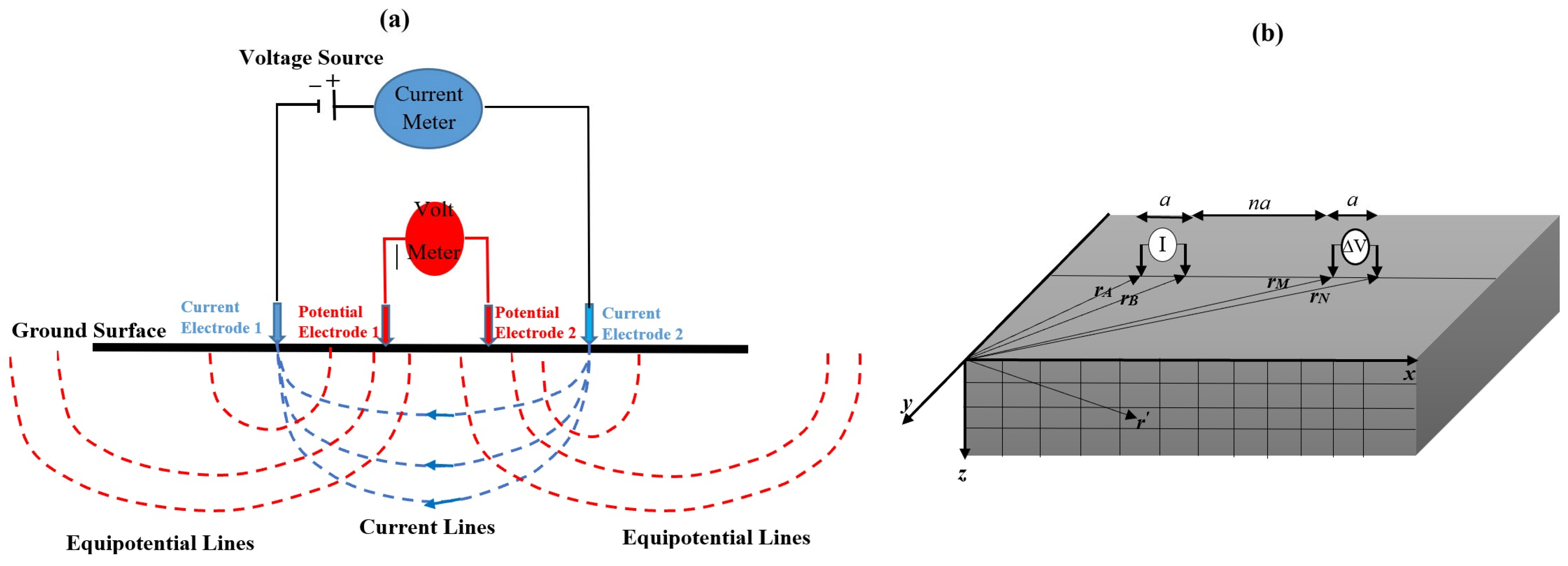
In this method, a DC or low-frequency alternating current is injected into the subsurface through a pair of current electrodes, while the resulting electrical potential difference is measured between a second pair of electrodes through a voltmeter (Figure 2a). From the measured electrical current and potential difference, the apparent resistivity of the subsurface is calculated by taking the distances between the four electrodes into account and by assuming that the subsurface is a homogeneous half-space. In this study, the forward problem is framed as a precision tool for structural reliability.
Various electrode geometries are employed during DC resistivity surveys, among which the dipole–dipole array (Figure 2b) is one of the more commonly used configurations. In this array, the current and potential electrode pairs (dipoles) are separated by a distance that is a multiple n of the dipole lengths a .
Resistivity surveys are generally conducted via two primary strategies: profiling, which maps lateral variations in lithological resistivities, and sounding, in which vertical changes in the resistivities of subsurface layers are investigated. The integration of sounding and profiling enables a two-dimensional (2D) investigation of the subsurface, known as electrical resistivity tomography (ERT). Therefore, electrical resistivity tomography surveys aim to determine the subsurface resistivity distribution both horizontally and vertically by making measurements on the ground surface [38], serving as a robust NDT tool for engineering site characterisation.
The basis for DC resistivity modelling using the integral equation method lies in the classical scattering equations derived from Maxwell’s equations at zero frequency. In this framework, a given model consists of the background medium and the anomalous zone. The background medium serves as the reference framework, while the scattered field generated by the anomalous zone is computed as the forward response. Although Maxwell’s equations are inherently nonlinear with respect to the electrical conductivity, Pérez-Flores, Méndez-Delgado and Gómez-Treviño [24] introduced a linearised relationship between the logarithm of apparent resistivity and the logarithm of true resistivity using a linear approximation. Consequently, the integral form of this forward problem is expressed as a Fredholm Integral Equation of the First Kind (IFK). The 2D forward formula in integral equation form is:
d s = A s , x , z   m x , z   d x d z
where s represents the current and potential electrodes, d is a forward response, ( x , z ) are coordinates of the points of the area of interest, A is the kernel and m is the subsurface model expressing the log10 of resistivity or conductivity distribution.
If the subsurface is divided into n x × n z cells, the discretised matrix equation is as follows:
d = A m  
where the kernel for DC current is defined as [24]:
A = n n + 1 n + 2 a 4 π ( I A M I A N I B M + I B N )
and
I i j = 4 c 2 + p 2 E q 8 p 2 K ( q ) c p 2 ( c 2 p 2 ) 2   x S t z 2 + c 2 4 U c 3 q               f o r       c > p   .   q = c 2 p 2 c 2   4 c 2 + p 2 E q 8 c 2 K ( q ) p c 2 ( p 2 c 2 ) 2   x S t z 2 + p 2 4 U p 3 c               f o r       p > c   .   q = p p 2 c 2 p 2 π 4 1 c 3 1 c 5 x S t z 2   .                                                                   f o r       c = p  
with
c 2 = ( x x S ) 2 + z 2
p 2 = ( x x ) 2 + z 2
U = E ( q ) q ( 1 q 2 ) E q q
x S t = ( x x S ) ( x x )
In the above expressions, i denotes the current electrode (A or B), and j represents the potential electrode (M or N). The variables x S and x represent the horizontal coordinates of the current and potential electrodes, respectively, while x and z indicate the coordinates of the cell centres. The functions K ( q ) and E ( q ) are the complete elliptic integrals of the first and second kind, respectively. The matrix A and vector m denote the forward operator and model parameters, with Equation (2) defining the forward problem. This formulation provides a numerically stable implementation for inversion, which is essential for obtaining reliable and interpretable results across various geoscience and engineering applications.

2.1.2. FDEM Surveying at Low Induction Numbers (LIN)

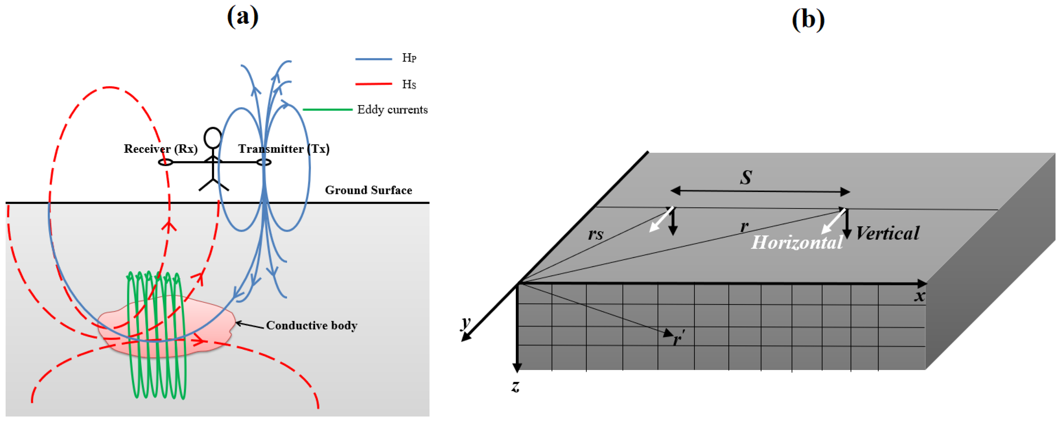
Generally, FDEM methods utilise time-varying currents to generate a primary magnetic field (HP) around a transmitter coil (TX). According to Faraday’s law, eddy currents are induced when this time-varying magnetic field intersects a conductive body within the Earth. These currents, in turn, generate a secondary magnetic field (HS) as described by Ampere’s law (Figure 3a). The receiver coil (RX) detects both the primary and secondary magnetic fields. The total magnetic field (HT) recorded by the receiver is the sum of the primary (HP) and secondary (HS) magnetic fields.
A typical survey layout is illustrated in Figure 3b, where S denotes the distance between the transmitter and receiver coils. Measurements of the magnetic fields may be made using different coil orientations: vertical coils correspond to horizontal magnetic dipoles (white arrows in Figure 3b), while horizontal coils correspond to vertical magnetic dipoles (black arrows in Figure 3b).
The speed, accuracy, high data volume, and non-destructive nature of FDEM methods have led to their widespread application in characterising the electrical conductivity and magnetic permeability of near-surface structures [21,48]. Within integrated geoscience investigations, these electromagnetic methods are referred to by various names, such as loop–loop methods, electromagnetic induction (EMI), or conductivity meters. Under specific conditions, they are classified as Low Induction Number (LIN) methods.
In the LIN regime, operating frequencies are chosen so that the inter-coil spacing is significantly smaller than the skin depths of the generated EM waves. FDEM systems operating at LIN are commonly used to map variations in the apparent electrical conductivity of the subsurface. In these methods, it is assumed that the Earth’s magnetic permeability is equal to the magnetic permeability of free space, and displacement currents are neglected. The Geonics EM34 system utilised in this study is a representative example of an FDEM system operating under the LIN approximation.
The interpretation of FDEM data can be categorised as either qualitative or quantitative. Qualitative interpretation involves analysing apparent conductivity and magnetic permeability data to estimate the approximate location and surface geometry of anomalous features in the subsurface. However, this approach does not provide information about the depth, overall geometry, or detailed electromagnetic properties of the target, such as conductivity and magnetic permeability. Consequently, various inversion techniques have been developed to model the subsurface distribution of electromagnetic properties. Such quantitative interpretation is essential for achieving the high-fidelity subsurface models required for complex geoscience and engineering investigations.
For the LIN technique, the kernel matrix of Equation (2) has been defined for the vertical magnetic dipole (VMD) and horizontal magnetic dipole (HMD) modes as follows [17,19]:
A V M D = s π y 2 x x x x s r r 3 r r s 3
A H M D = s π { 1 ρ 1 2 z + h ρ 1 2 r r y 2 ρ 1 2 C 1 1 ρ 2 2 z + h ρ 2 2 r r s y 2 ρ 2 2 C 2 x x ρ 1 2 C 1 x x s y ρ 2 2 C 2 }
where
ρ 1 2 = x x 2 + y 2 ,
ρ 2 2 = x x s 2 + y 2 ,
C 1 = 2 ρ 1 2 + 2 h z ρ 1 2 r r + h z r r 3 ,
C 2 = 2 ρ 2 2 2 z + h ρ 2 2 r r s z + h r r s 3
where r and r denote the position vectors of the observation point and the subsurface cell, respectively, while r s represents the source position. The variables x , y , and z correspond to the coordinates of the observation point, and x , y , and z denote the coordinates of the subsurface cell centres. The parameter h represents the height of the instrument above the ground surface.
By using these kernels within the framework of Equation (2), the apparent electrical conductivities can be forward modelled for various subsurface conductivity distributions. It is important to note that for background conductivities exceeding approximately 10 mS/m, the LIN approximation for the EM34 system begins to lose validity. Under these conditions, the induced secondary magnetic field is no longer negligible compared to the primary field, leading to nonlinear effects and potential inaccuracies in the estimated apparent conductivity.
To mitigate these effects, a correction proposed by Parnow, Oskooi and Florio [21] was applied. In this study, this correction was implemented for both synthetic and field datasets to improve the estimation of apparent conductivity. This is important for subsurface characterisation in geoscientific and engineering investigations, where consistent physical property mapping supports informed decision-making.

2.2. Separate and Cooperative Inversions

The methodology presented here integrates individual inversion algorithms into a structured sequential cooperative approach for improved subsurface characterisation. This process is divided into two primary stages: an individual inversion based on a damped weighted minimum length solution [21,25], followed by a cooperative inverse process to resolve ambiguities and improve the fidelity of the final models.

2.2.1. Inversion Methodology

As previously detailed, Pérez-Flores, Méndez-Delgado and Gómez-Treviño [24] established a linear integral equation approach for DC resistivity and EM-LIN methods based on the Born approximation. Equations (3), (5) and (6) represent the kernel functions, which depend on the geometry of configurations used during data collection for both methods. To facilitate rigorous numerical modelling, Equation (2) is discretised so that the subsurface is divided into many prisms with infinite extent along one direction (y). The midpoint rule is applied to this discretisation, allowing Equation (2) to be solved as a system of linear equations in matrix form.
The inherent non-uniqueness and instability of geophysical inverse problems, critical factors in reducing uncertainty within subsurface investigations, require the inclusion of a priori information and physical constraints. These are incorporated into the inversion procedure through regularisation. Following the approach proposed by Tikhonov and Arsenin [49], we define the objective function as:
m i n W d A m d 2 2 + α W m m m 0 2 2
where the left-hand term describes the data misfits, weighted by the data covariance matrix W d , while the right-hand term denotes the model objective function, weighted by the model weighting matrix W m . The vector m 0 expresses the initial model, which can be constructed using a priori information, such as geological constraints or results from complementary geophysical datasets. The regularisation parameter α controls the relative contribution of the second term in the inverse model; high values of α increase the model bias and decrease resolution, thereby increasing the RMS error of the data misfit.
Over the past decades, various algorithms have been proposed for the independent inversion of DC resistivity and EM-LIN data [24,50,51,52,53,54]. In this study, a damped weighted minimum length solution algorithm is used for the inversion of DC resistivity and EM-LIN data, following the methodologies established by Varfinezhad, Oskooi and Fedi [11] and Parnow, Oskooi and Florio [21]. This approach incorporates both regularisation and depth weighting, which help stabilise the inversion process by mitigating the effects of noise and non-uniqueness, leading to more reliable subsurface models.
m = m 0 + W m 1 A T A W m 1 A T + α W d 1 d A m 0
where W m is assumed to be a depth weighting function, a technique pioneered by Li and Oldenburg [55,56] for potential methods to maintain high fidelity at depth. Since its inception, depth weighting has been widely used in potential field data inverse algorithms [57,58,59,60]. The iterative method terminates when there is no discernible improvement in data misfit with each iteration. To evaluate the quality of the fit, the normalised Root Mean Square (RMS) error is utilised, defined as [41]:
N o r m a l i z e d   R M S   e r r o r   % = 1 N i = 1 N d o b s , i d p r e d , i σ i 2 M e a n ( d o b s ) × 100
where d o b s , i represents the ith observed data point, and d p r e d , i is the ith computed data point derived from the current model. The variable σ i represents the standard deviation of the observed data point, and N denotes the total number of data points. The iterative inversion approach proposed in this study utilises the convergence of the data misfit as a primary stopping condition; this prevents overfitting and improves the geophysical fidelity and reliability of the final subsurface model.

2.2.2. Sequential Cooperative Inversion Framework

In this study, cooperative inversion is implemented by adopting the inverse model of one method as the initial constraint for the other, and vice versa. During each iteration, individual inversions of both datasets are performed. Specifically, the output of one method, say DC resistivity, is used as the input for the inversion of the other method (EM34); simultaneously, the resulting EM34 model serves as the initial model for the DC resistivity inversion.
It should be mentioned that individual inversions of both methods are maintained by updating their respective initial models without mutual information sharing. This parallel approach provides four distinct inverse models for comparison: (1) individual inversion of DC resistivity, (2) individual inversion of EM34, (3) cooperative inversion of DC resistivity, and (4) cooperative inversion of EM34. The efficacy of the adopted individual inversion algorithm has been demonstrated in previous literature across various synthetic and field cases for both methods (e.g., [12,21,24,61]).
Joint inversion of different configurations of the EM34 technique requires a balanced objective function to improve the final model, which is not dominated or biased toward a single configuration. A similar challenge is reported in the literature about the combination of different geo-electrical arrays [62]. In this study, to combine the inversion of both arrays of the LIN technique (VMD and HMD), a weighting factor is employed to equalise the contributions of the data of each array. We adopted a technique developed for electrical resistivity to different arrays based on sensitivity/Jacobian matrices [62].
By iteratively updating the initial models through mutual information sharing, the sequential cooperative inversion addresses the non-uniqueness challenges typical of individual methods. This integrated workflow is particularly effective in resolving complex structural targets, such as the hydrogeologically significant dolerite dykes investigated in this study, by integrating the complementary lateral sensitivity of FDEM with the vertical resolution of DC resistivity.

3. Benchmark Validation and Geoscience–Engineering Application

To evaluate the performance of the proposed cooperative inversion technique, the methodology is applied to two distinct synthetic benchmarks and a high-priority field site. This multi-staged validation supports both the numerical stability of the algorithm and its practical efficacy for complex subsurface investigations.

3.1. Synthetic Model I: Multi-Modal Sensitivity Assessment

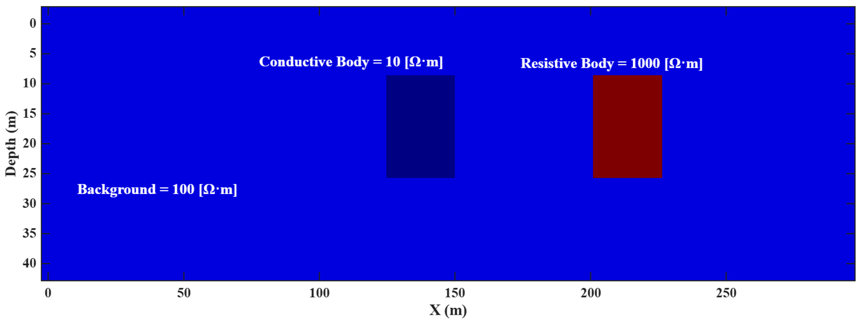
The first synthetic model serves as a rigorous test of the algorithm’s ability to resolve contrasting electrical properties within a homogeneous background medium (100 Ω·m). The model is characterised by two distinct anomalous bodies: one conductive (10 Ω·m) and one resistive (1000 Ω·m).
These significant contrasts support that the model poses a non-trivial challenge for inversion algorithms (Figure 4). Furthermore, the spatial configuration and contrasting electrical properties of these two bodies allow for a comprehensive assessment of the proposed technique’s ability to resolve and distinguish subsurface features under realistic conditions. The model domain spans 300 m in the horizontal (x) direction and 40 m in the vertical (z) direction. It is discretised into a high-resolution numerical mesh of 2 m × 2 m square prisms, resulting in 150 cells along the x-axis and 20 cells along the z-axis.
This model has been used in previous studies as a benchmark for evaluating geophysical inversion methods [61,63], and its moderate complexity makes it well-suited for examining both robustness and accuracy. Subjecting the proposed sequential cooperative inversion method to this established synthetic scenario allows for a meaningful comparison with existing approaches and demonstrates its effectiveness in resolving complex subsurface resistivity distributions. This configuration poses a non-trivial challenge for standard inversion algorithms, as it requires the simultaneous resolution of steep resistivity gradients, a critical capability for reliable site characterisation in geologically variable environments.

3.2. Synthetic Model II: Structural Boundary Definition

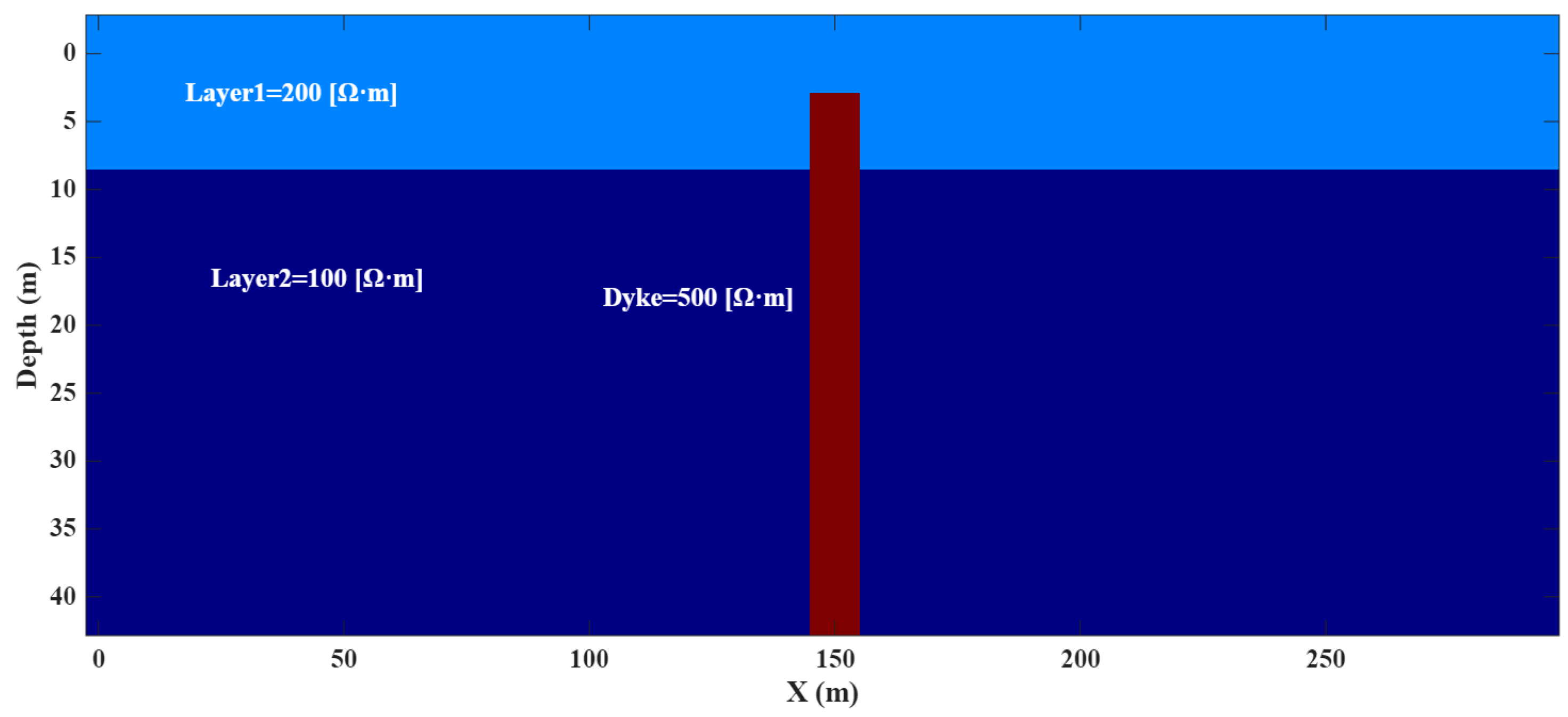
For the second synthetic test, we considered a model domain measuring 300 m horizontally and 40 m in depth, featuring a vertical dyke within a two-layered medium (Figure 5). The dyke extends from 5 m to 10 m beneath the surface, providing a realistic scenario for evaluating the ability of the inversion scheme to detect and characterise discrete subsurface structures.
The first (upper) layer of the medium was assigned a resistivity of 200 Ω·m, while the second (lower) layer was set at 100 Ω·m (Figure 5). In contrast, the vertical dyke was modelled with a resistivity of 500 Ω·m. The numerical mesh was discretised into 150 cells in the horizontal direction and 20 cells in the vertical direction, yielding rectangular prisms each measuring 2 m × 2 m.
Synthetic apparent resistivity data were generated using the dipole–dipole configuration with electrode spacings ranging from 5 m, resulting in 804 data points. Additionally, 308 stations were modelled along the profile for the EM-LIN data for both arrays, with measurements acquired at 5 m intervals between stations.
This second synthetic model was designed to test the robustness of the inversion technique in resolving both horizontal layer boundaries and relatively narrow vertical features, thus providing a thorough assessment of the algorithm’s capacity to handle complex subsurface conditions. In the context of integrated geoscience and engineering investigations, the ability to resolve such vertical discontinuities is crucial for non-destructive characterisation, where precision in locating structural boundaries is essential for the comprehensive assessment of subsurface stability and composition.

3.3. Field Data: Morgenzon Farm, South Africa

To demonstrate the practical applicability of the sequential cooperative framework, the algorithm was applied to real-world datasets acquired at the Morgenzon Farm site in South Africa. The site represents a relevant case study for both geoscientific interpretation and subsurface engineering investigations, particularly in identifying structural features such as dolerite dykes with significant hydrogeological implications [64]. The datasets consist of co-located DC resistivity and EM34 profiles.
Dolerite dykes are important targets for groundwater exploration in the Karoo region due to their hydrogeological significance, often acting as barriers or conduits for water flow [65]. Given the high resistivity contrast between these igneous structures and the surrounding sedimentary formations, resistivity-based geophysical methods such as DC resistivity and EM34 are exceptionally well-suited for their detection as part of a non-destructive characterisation campaign.
The field investigation utilised a high-density data acquisition strategy:
  • EM34 Data: Collected using both VMD and HMD configurations along a 400 m profile. Measurements were recorded at 10 m intervals, using transmitter–receiver (T-R) separations of 10, 20, and 40 m to capture varying depths of investigation.
  • DC Resistivity Data: Acquired using a Wenner–Schlumberger array with two distinct acquisition schemes, employing electrode spacings of 5 m and 10 m along the same profile to provide different resolution and depth of investigation, resulting in 900 discrete data points. While dipole–dipole arrays are generally more sensitive to lateral resistivity variations, the Wenner–Schlumberger array was selected for its superior robustness and data stability under local field conditions.
This multi-modal field application demonstrates the effectiveness of the proposed methodology for resolving complex subsurface geometries. By integrating qualitative site observations with quantitative structural modeling, this field case serves as a benchmark for reducing uncertainty in large-scale infrastructure planning and strategic resource management.

4. Results

The performance of the proposed sequential cooperative framework was evaluated through comparative analysis against individual inversion results for two synthetic benchmarks and a high-fidelity field dataset.

4.1. Separate and Cooperative Inversion of Synthetic Datasets

As previously established, a homogeneous initial model was used for the individual inversions of both DC resistivity and EM34 datasets, based on the background properties of the synthetic models. In contrast, the cooperative approach iteratively updates the initial model by incorporating structural and resistivity information from the complementary dataset.

4.1.1. Synthetic Model I

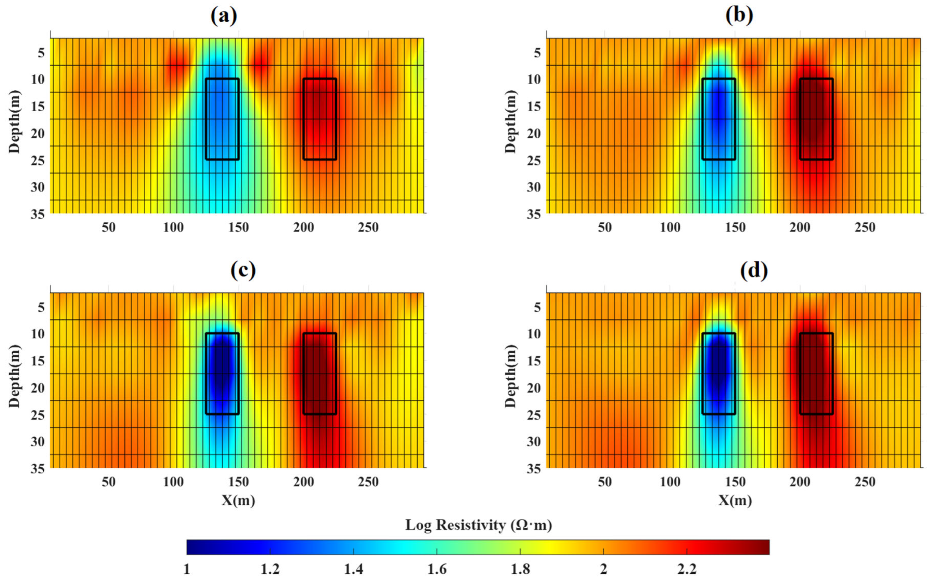
Figure 6 presents the comparative inverse models for Synthetic Model I. The individual inversions of EM34 and DC resistivity data were executed using the linear integral formulation described by Pérez-Flores, Méndez-Delgado and Gómez-Treviño [24], combined with the inversion scheme adopted in this study [12,21]. The independent DC resistivity inversion (Figure 6b) provides a more detailed reconstruction of the subsurface compared to the EM34 inversion (Figure 6a); this is consistent with the inherently higher spatial resolution of DC methods in shallow investigations. However, both individual inversion results show limitations in recovering the full geometry and amplitude of the anomalies.
The cooperative inversion results indicate that both methods benefit from the integration of complementary information. The EM34 inversion (Figure 6c) shows a more pronounced improvement in defining the anomaly boundaries. Similarly, the cooperative inversion of the DC resistivity data (Figure 6d) improves the reconstruction relative to its individual counterpart, yielding results that are more consistent with the true model in both synthetic cases.
In contrast, the cooperative joint inversions (Figure 6c,d) show improved imaging results and amplitude representation compared to the individual inversions. By integrating the complementary sensitivities of both methods, the proposed framework provides an enhanced representation of both conductive and resistive anomalies. This technique shows improved performance compared to individual inversions by addressing both types of anomalies, indicating its potential for generating reliable geophysical models in complex geological settings.
Figure 7 illustrates that, in general, the RMSE decreases with the number of iterations across all inversion scenarios. The cooperative inversions in Figure 7c,d converge in fewer iterations than their individual counterparts Figure 7a,b, indicating enhanced convergence efficiency. In Figure 7c, the RMSE for the EM34 data decreases from 1% to approximately 0.7%, while in Figure 7d, the DC resistivity RMSE decreases from 4.38% to 4.28%. Although the final RMSE values of the individual and cooperative inversions are comparable, the cooperative framework achieves similar levels of data misfit in fewer iterations. This suggests that a primary advantage of the cooperative inversion lies in its convergence behaviour and the stabilisation of the inverse problem, rather than a reduction in final RMSE.
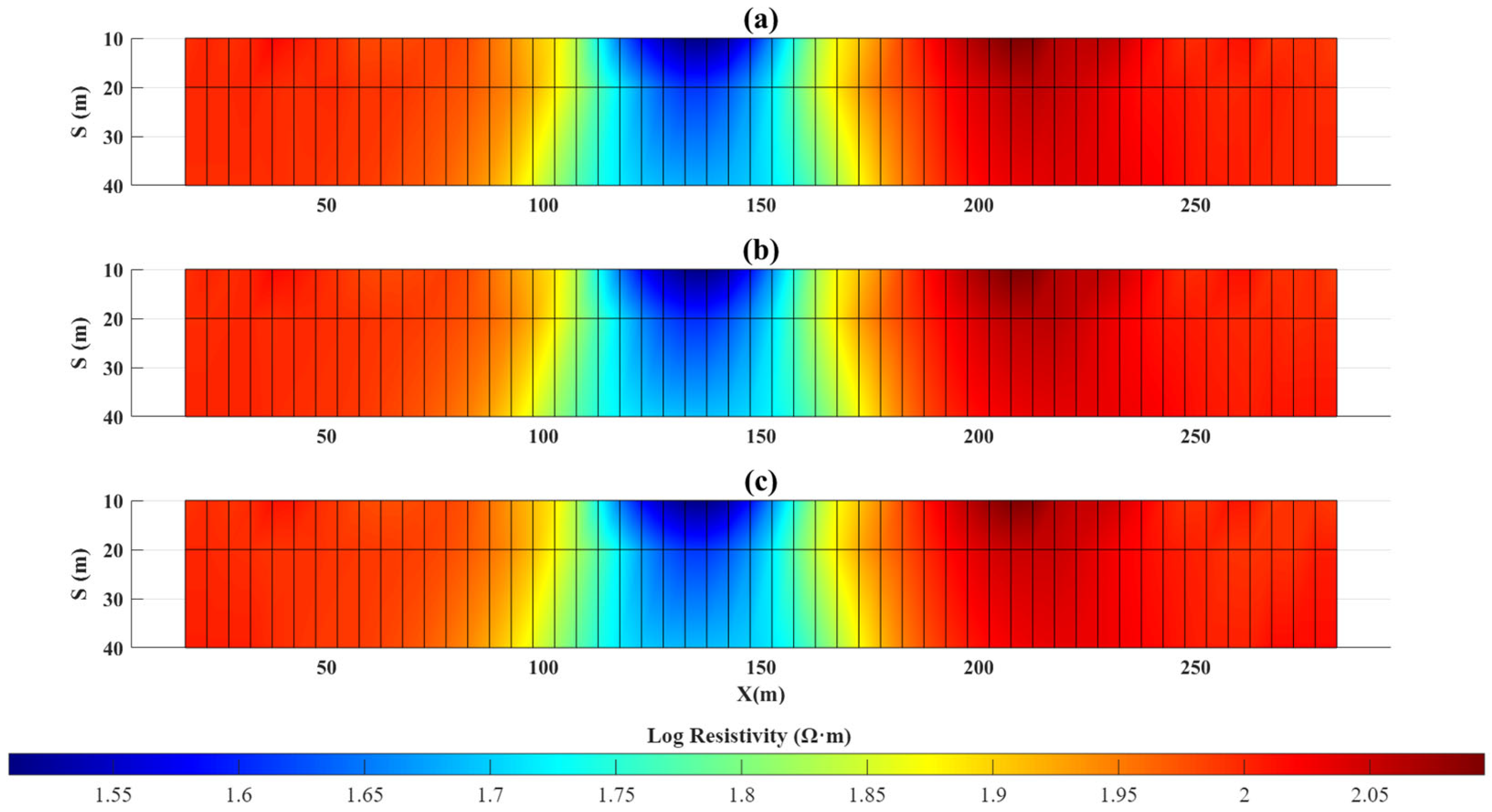
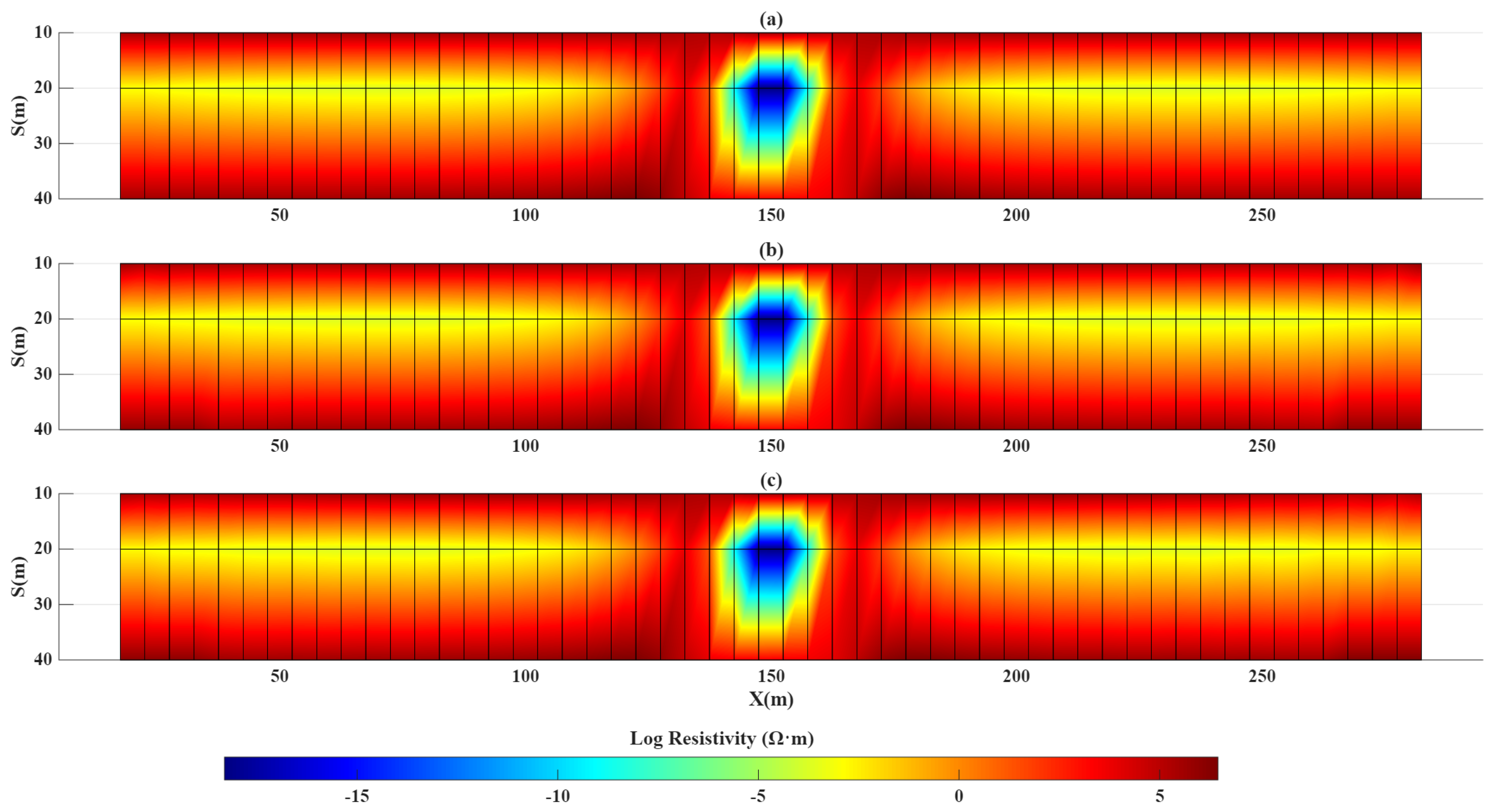
Figure 8 and Figure 9 compare the synthetic input model’s apparent resistivity data with the calculated pseudo-sections generated from both individual and cooperative inversions for Synthetic Model I. In Figure 8, the input model (Figure 8a) appears visually similar to the calculated responses of the individual (Figure 8b) and cooperative (Figure 8c) inversions. Quantitatively, however, the cooperative inversion yields a slightly lower RMSE (0.75%) compared to the individual inversion (0.8%), indicating a marginal improvement in the data fit for the EM34 method.
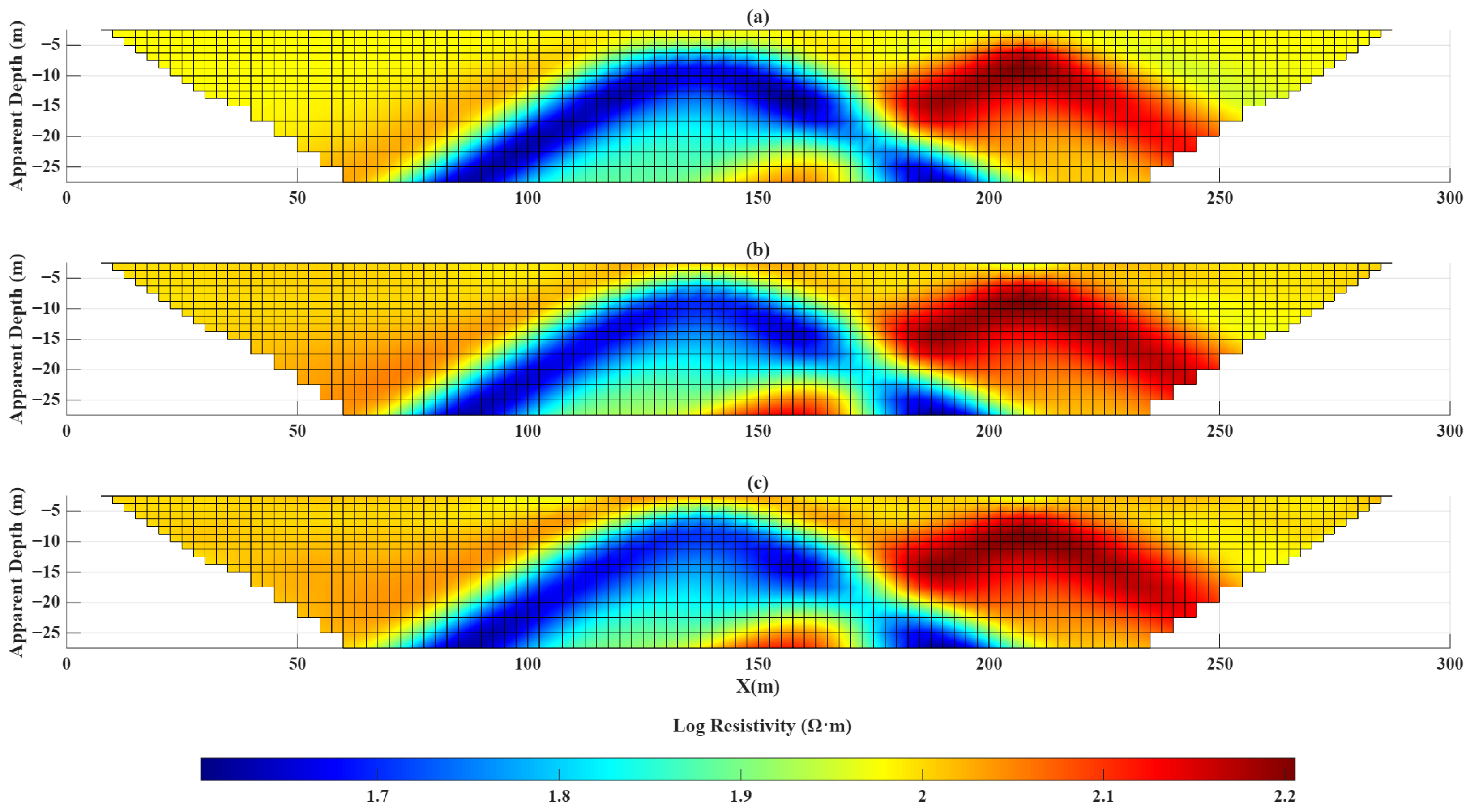
Similarly, in Figure 9, the electrical resistivity pseudo-sections show comparable patterns across the input model, individual inversion, and cooperative inversion. Nevertheless, the RMSE values demonstrate that the cooperative approach (3.5%) achieves a lower misfit compared to the individual inversion (4.3%), despite the visual similarities in the pseudo-sections. These results indicate that sequential information sharing within the cooperative inversion framework successfully refines the subsurface reconstruction and provides a more robust fit to the observed data.
This methodology uses the integration of complementary datasets to generate subsurface models with improved resolution and greater accuracy. The findings underscore the framework’s reliability and its substantial potential for enhanced subsurface modelling compared to conventional individual inversion methods. Ultimately, these results indicate that the proposed cooperative approach improves the consistency of subsurface imaging, supporting more reliable and robust interpretation in both geoscientific and engineering investigations.

4.1.2. Synthetic Model II

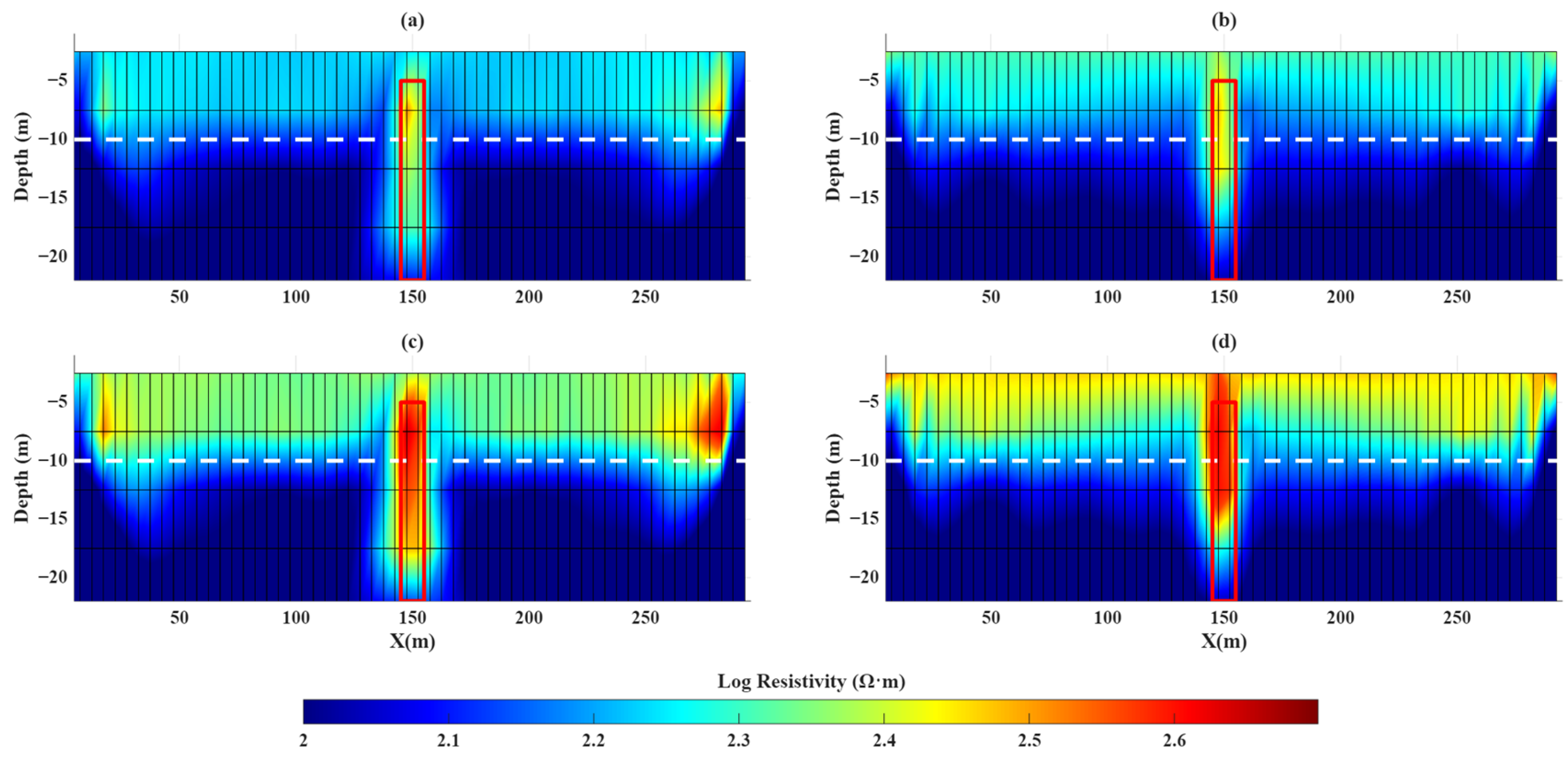
Figure 10 presents the comparative results of the separate and cooperative inversions of EM34 and electrical resistivity data for the second synthetic benchmark. In the separate inversions (Figure 10a,b), although a central vertical resistive anomaly is present, its geometry appears diffuse, and the structural boundaries are poorly resolved. Similarly, while the first layer (Layer 1) exhibits the expected higher resistivity, its resistivity distribution is not well-defined, and the boundary at the base of this layer remains indistinct. These limitations highlight the inherent challenges of delineating subsurface features using separate inversion methods, which often lack the resolution required to resolve discrete vertical discontinuities and sharp interfaces simultaneously.
In contrast, the cooperative joint inversion results (Figure 10c,d) exhibit a marked improvement in model clarity and structural fidelity. By iteratively sharing mutual information, the framework enables the identification of the vertical dyke, with improved boundary definition and better-resolved resistivity contrast relative to the host medium. Furthermore, the interface between the upper and lower geological units, indicated by the horizontal white dashed line, is reasonably delineated. The thickness of the first layer is estimated with a reasonably good agreement, particularly when considering the smoothing effects typically inherent in regularised inversion results.
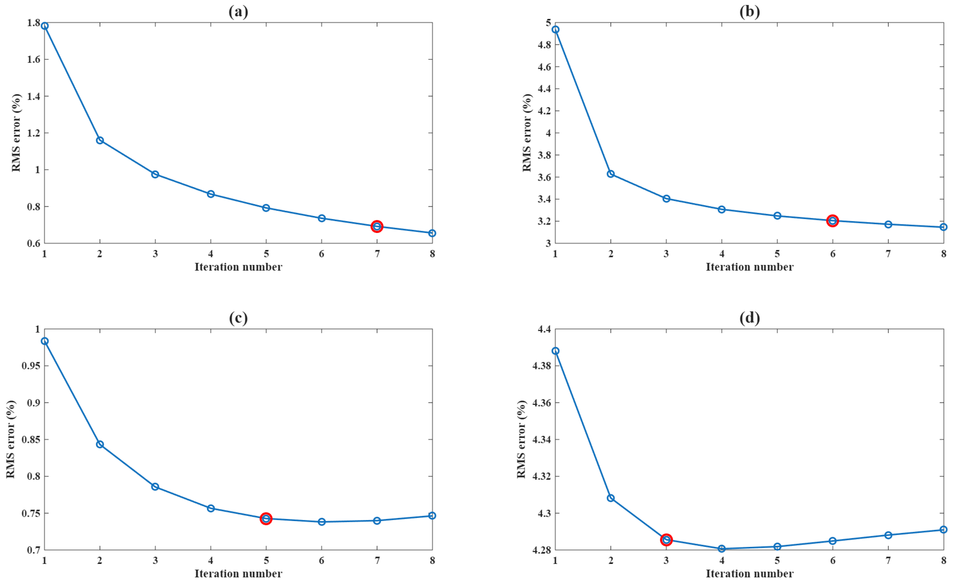
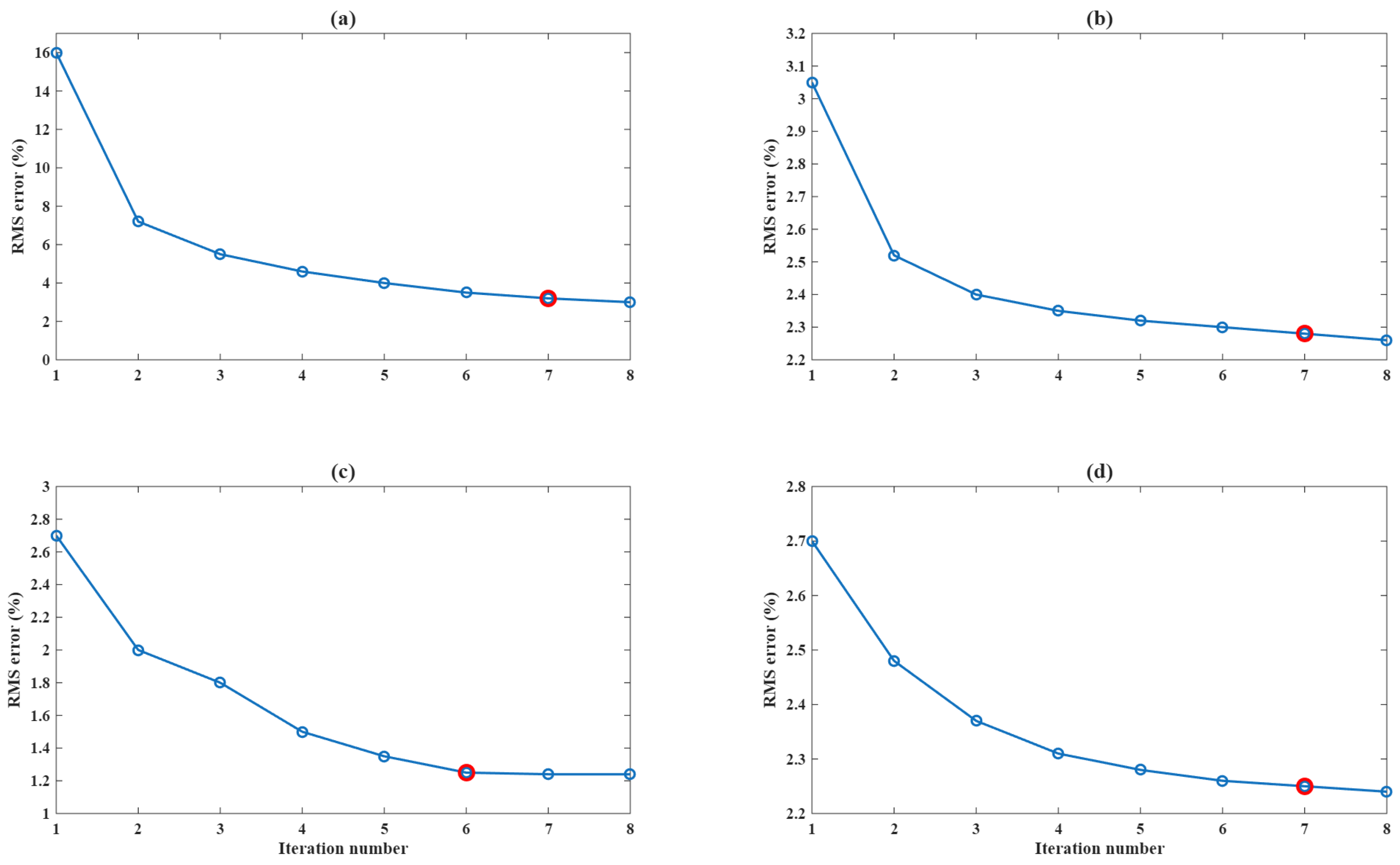
The variation in the RMSE over successive iterations for both separate and cooperative joint inversions of Synthetic Model II is illustrated in Figure 11. The red markers indicate the specific iteration at which the algorithm satisfies the convergence criteria and terminates. As shown in Figure 11a,b, the RMSE for the individual inversions decreases consistently with iterations; however, the convergence is noticeably slower, and the final residual error remains higher than that of the cooperative results.
In contrast, the cooperative framework demonstrates a more rapid decay in RMSE and achieves lower final values, indicating superior model fitting and computational efficiency. With the exception of the cooperative EM34 inversion, all algorithms reach convergence within seven iterations.
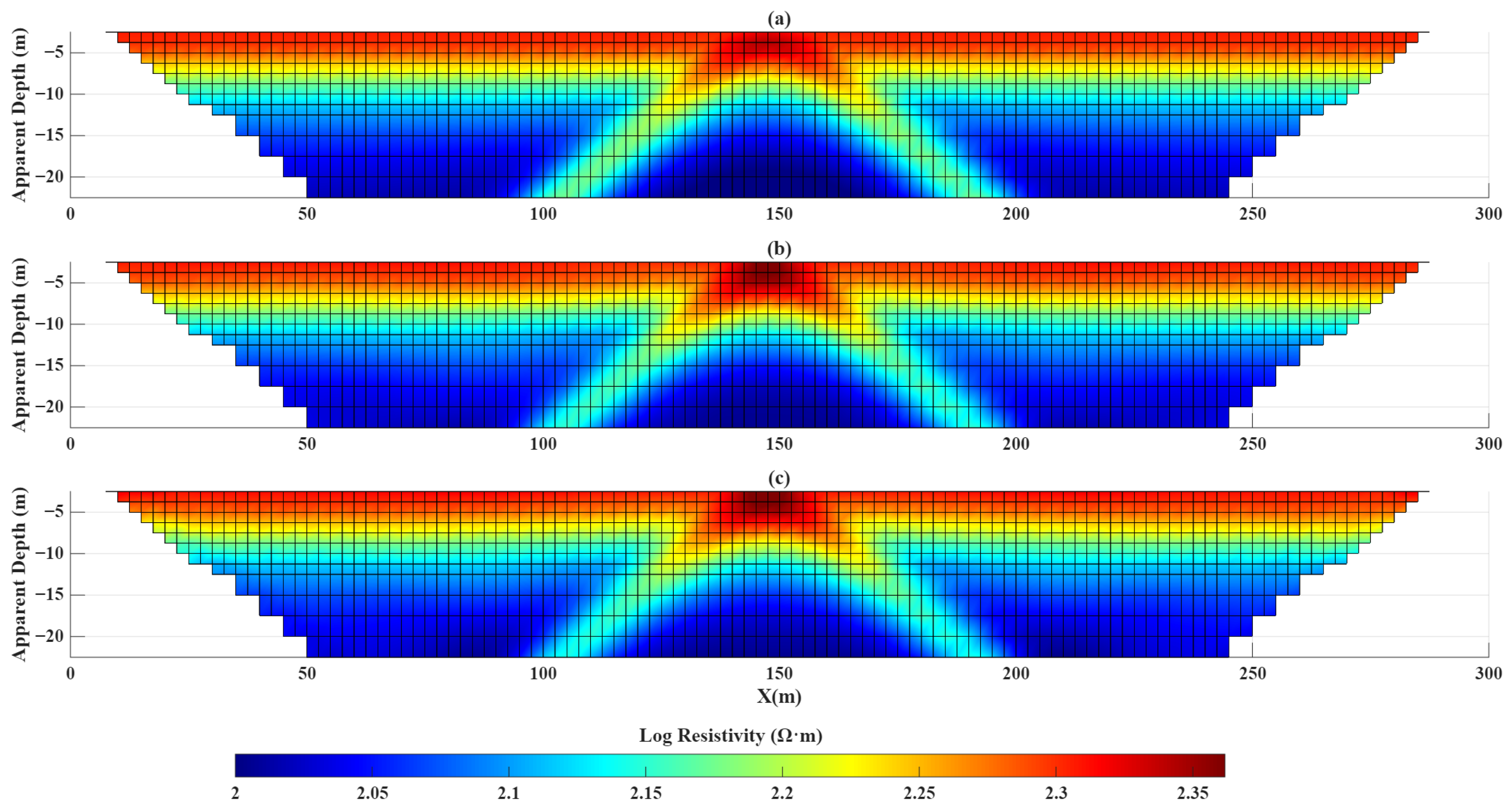
Figure 12 and Figure 13 present the synthetic pseudo-sections alongside the recovered data from the individual and cooperative inversions for the EM34 and DC electrical resistivity methods for Model II, respectively. For the EM34 technique, the cooperative inversion (Figure 12c) demonstrates improved agreement with the reference data compared to the individual inversion (Figure 12b). Similarly, the DC resistivity results (Figure 13) show that the cooperative approach (Figure 13c) reproduces the observed data more consistently than the individual inversion (Figure 13b). These qualitative comparisons of the pseudo-sections confirm that the integration of complementary datasets enhances the reconstruction of complex subsurface features.
This robust characterisation of both horizontal layer interfaces and narrow vertical discontinuities establishes the methodology as a high-performance non-destructive characterisation tool. Such results are important for integrated geoscience and engineering investigations, where the reliable identification of structural boundaries and data amplitude variations is essential for informed geological interpretation and engineering decision-making.

4.2. Separate and Cooperative Inversion of Field Data: Morgenzon Farm

The practical utility of the sequential cooperative framework was evaluated using field datasets acquired at Morgenzon Farm, South Africa. The study area has been previously investigated using integrated geophysical methods, including joint inversion of resistivity and gravity gradient data [3,66]. Additional site-specific geological and hydrogeological details are documented in earlier field reports.
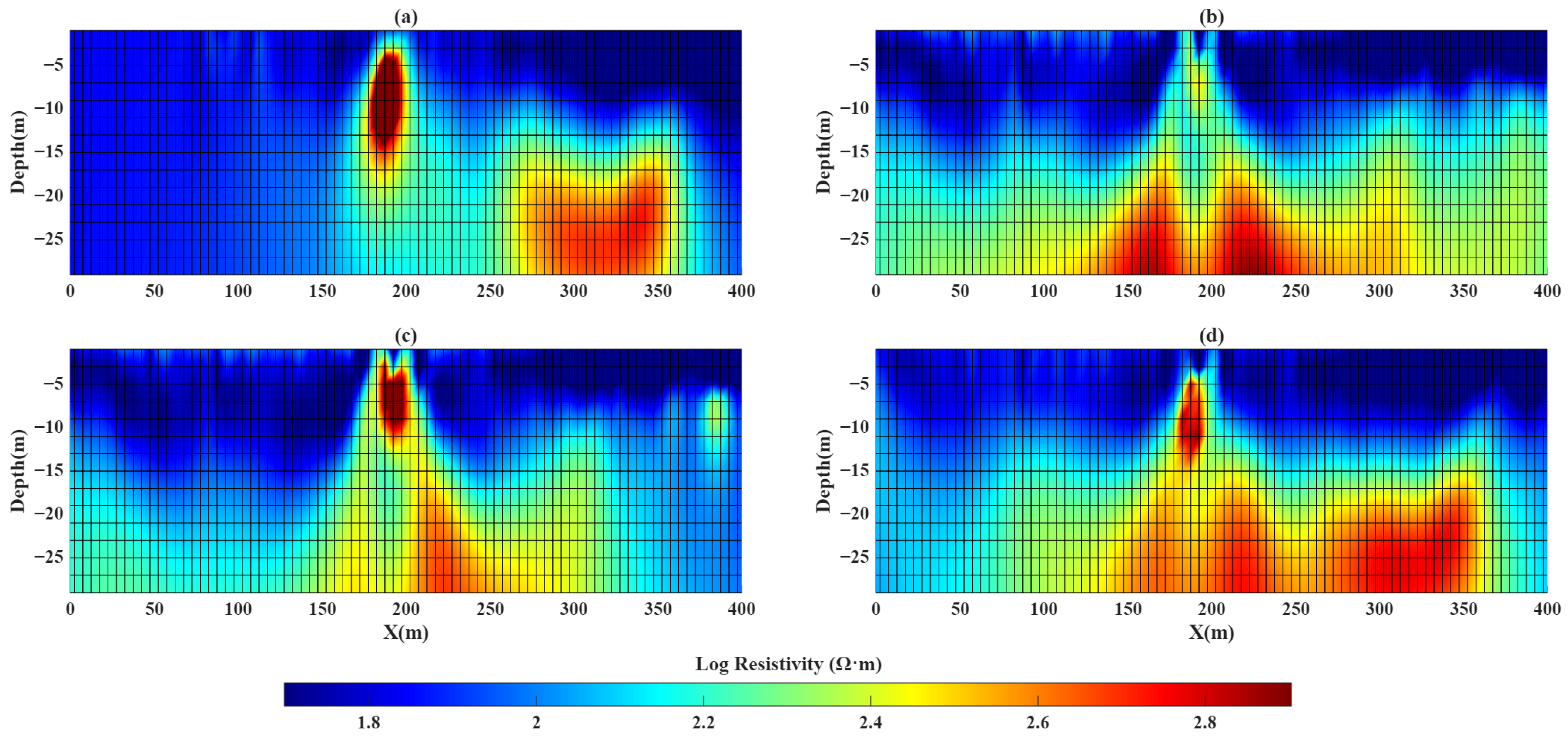
Figure 14 presents a comparative evaluation of the inverse models generated via separate and cooperative inversion strategies.
The individual EM34 inversion (Figure 14a) successfully identified a prominent vertical anomaly located horizontally between 180 m and 200 m marks along the profile. Within the geological context of the Karoo Supergroup, this feature is interpreted as a dolerite dyke. The inversion suggests the dyke originates at a depth of approximately 5 m and extends vertically to at least 15 m. Additionally, a resistive zone is observed between 270 m and 350 m, at depths ranging from 15 m to the lower boundary of the recovered model. However, the separate EM34 model provides limited resolution regarding the broader stratigraphic layering and the precise contact zones surrounding the intrusion.
In contrast, the separate DC resistivity inversion (Figure 14b) failed to delineate the dyke as a discrete vertical body. Instead, it primarily reconstructed a fluctuating horizontal interface boundary extending from the left toward the near-surface in the centre of the profile. While a small, thin anomaly is evident near the profile centre, within a 5 to 10 m depth range, the separate EM34 model provides limited resolution to define the broader stratigraphic layering and the precise contact zones surrounding the intrusion.
The sequential cooperative inversion of the DC resistivity data (Figure 14d) successfully resolves these discrepancies by effectively integrating the high lateral sensitivity of the EM34 data with the vertical resolution of the DC resistivity measurements. By sharing structural information across datasets, the framework clearly delineates both the sharp vertical boundaries of the dyke and the surrounding stratigraphy.
Specifically, the cooperative resistivity model derived from EM34 data, constrained by DC resistivity results (Figure 14c), represents an interface-dominated subsurface structure while preserving the resistive zone in the centre of the profile. The cooperative inversion of the DC resistivity data (Figure 14d) provides improved results, delineating both the stratigraphic interface and the dyke zone with greater clarity compared to the independent inversions. This indicates an enhanced representation of the subsurface structure.
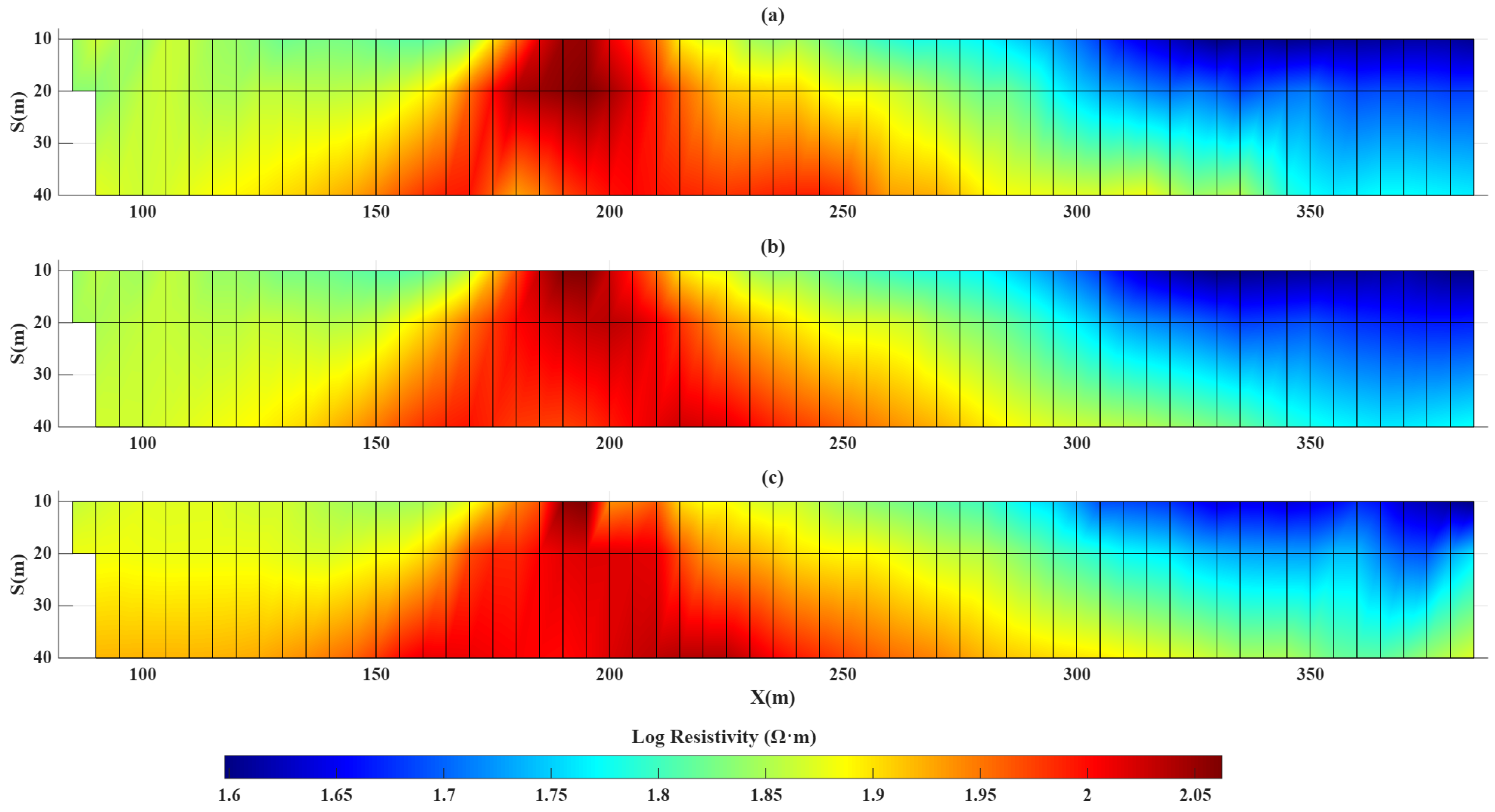
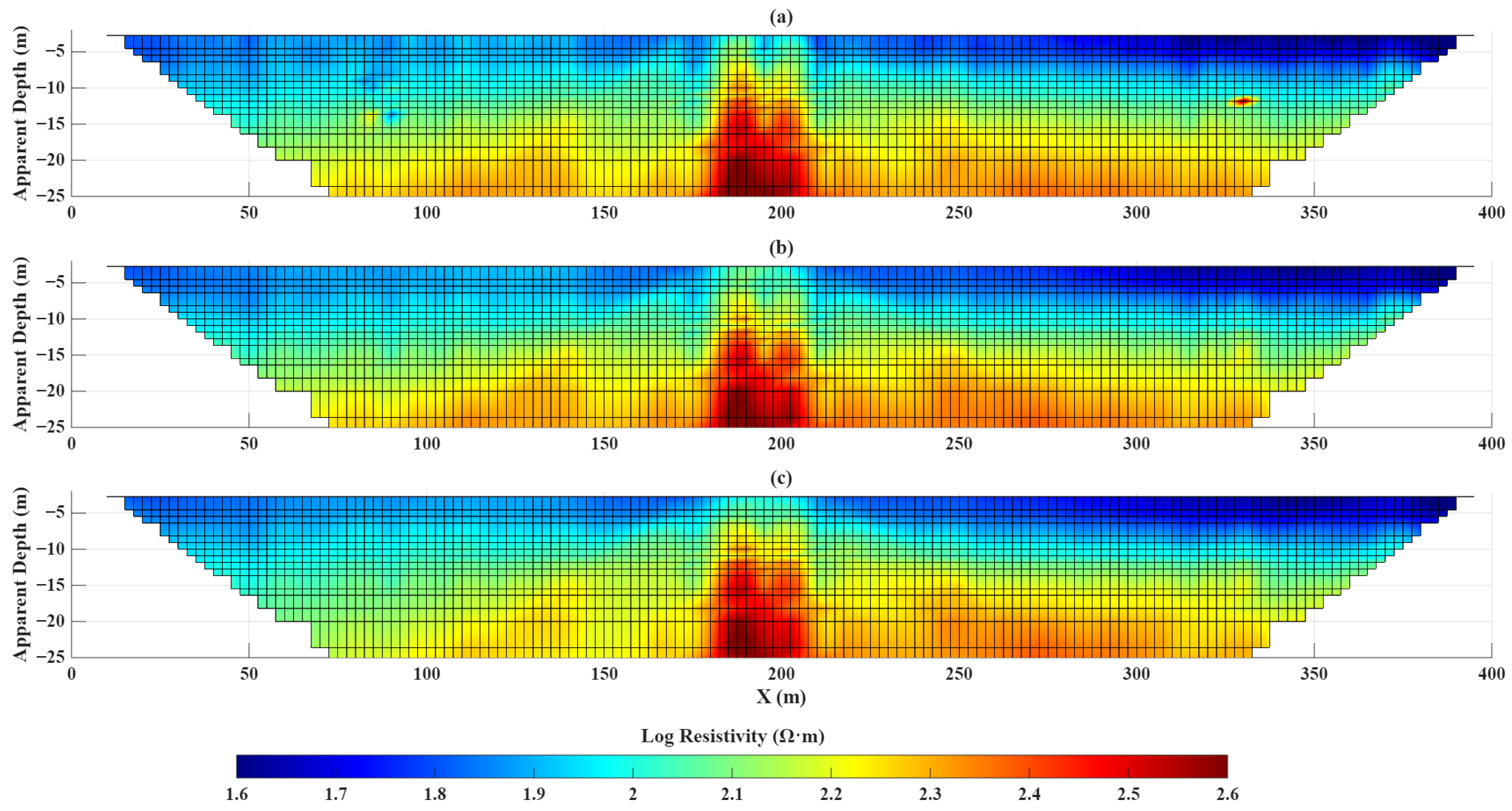
The measured and recovered datasets for both methods are presented in Figure 15 and Figure 16. These figures indicate the framework’s numerical stability and data-fitting capabilities, showing a high degree of correlation between field observations and the model-recovered values.
From a hydrogeological and engineering perspective, the resistive zone identified on the left side of the expected dyke may indicate reduced water content, as the dolerite dyke likely acts as a hydraulic barrier impeding lateral groundwater flow [64]. Consequently, the zones of lower resistivity on the opposite side of the dyke could correspond to zones with higher water content, making them high-priority targets for strategic water resource management and infrastructure planning.

5. Discussion

The synthetic inversion results rigorously demonstrate the efficacy of the sequential cooperative framework. This enhanced performance is primarily attributable to the strategic selection of the initial model through information sharing. To evaluate the fidelity of the inverted models against the synthetic (true) benchmarks, target reconstruction was quantified in terms of Geometry (spatial location and morphology) and Amplitude (resistivity contrast).
The geometry reconstruction (%) was assessed based on the spatial overlap between the true and inverted anomaly regions using:
G e o m e t r y = × t i t i × 100
where Ωt and Ωi represent the true and reconstructed anomaly regions, respectively.
The amplitude reconstruction (%) was quantified using a normalised L 2 -norm misfit within the true anomaly region:
A m p l i t u d e = 1 M t M i 2 M t 2 × 100
where Mt and Mi denote the true and inverted model parameters within the target zone, respectively. The use of normalised L 2 -norm misfit is consistent with standard practices in inverse problem theory [2,67].
The anomaly regions were defined using a threshold-based criterion, where values exceeding a specified fraction (e.g., 0.7) of the maximum or minimum of the true model were considered part of the target. For models containing both conductive and resistive anomalies, the reconstruction metrics were computed separately for each anomaly and subsequently averaged to provide a representative measure.
As shown in Table 1, a threshold-based criterion was employed to define the target boundaries, whereby values exceeding 0.7 times the maximum or minimum of the true model were considered part of the anomaly. For synthetic models containing both conductive and resistive anomalies, the reconstruction metrics were evaluated separately for each anomaly and subsequently averaged to provide a representative assessment of the inversion performance. The anomaly region was defined using a relative threshold of 0.7 times the maximum or minimum value of the true model, following commonly adopted practices in synthetic inversion studies [63]. This threshold was selected to capture the core of the anomaly while minimizing the influence of transition zones introduced by inversion smoothing.
The quantitative analysis in Table 1 confirms that the cooperative framework significantly enhances the RMSE relative to separate inversion strategies. Furthermore, the framework consistently outperformed individual methods in reconstructing both the geometry and amplitude of target anomalies:
  • In Model I, cooperative inversion improved amplitude recovery from 88% to 96% for the EM34 method and from 85% to 97% for the DC electrical resistivity method. Geometry reconstruction similarly advanced from 78% to 85% and from 77% to 87%, respectively.
  • In Model II, the framework yielded amplitude improvements from 80% to 95% (EM34) and 82% to 95% (resistivity), along with geometry enhancements from 75% to 84% and 75% to 88%.
These results indicate that the cooperative inversion approach improves the reconstruction of structural morphologies and physical contrasts compared to standalone methods. This improvement is generally achieved with a comparable or only slightly increased computational cost, reflecting the efficiency of the framework despite the additional complexity of integrating complementary datasets. All computations were performed on a standard desktop computer (Intel(R) Core (TM) i5-10210U, 1.60 GHz, 16 GB RAM), demonstrating the practical feasibility of the proposed method for routine geoscientific and engineering investigations.
The field application at Morgenzon Farm provides further insights into the practical utility of the sequential framework. For the EM34 data, the integration of DC resistivity results as a structural constraint facilitated the reconstruction of the stratigraphic interface zone, which was poorly resolved in the standalone EM34 inversion. Conversely, the cooperative inversion process improves the DC resistivity results; the interface zone is preserved, while the vertical dyke structure, previously less clear or distorted in the independent resistivity model, is more clearly represented.
This result indicates that the sequential cooperative inversion approach integrates the complementary strengths of EM34 and DC resistivity methods, providing an enhanced and more consistent representation of subsurface structures.

6. Conclusions

This research has successfully established and validated a robust sequential cooperative inversion framework, integrating DC resistivity and EM34 data to enhance the fidelity of subsurface electrical resistivity imaging. The methodology was rigorously tested through synthetic benchmarks and successfully deployed at the Morgenzon Farm site in South Africa, specifically targeting the detection and characterisation of dolerite dykes, critical structural features in hydrogeological and engineering contexts.
The efficacy of the proposed methodology was rigorously confirmed through three primary findings:
  • In synthetic benchmarking, the cooperative framework demonstrated a clear advantage in simultaneously recovering conductive and resistive anomalies. For Synthetic Model I, it achieved substantial improvements in both RMSE, target geometry and amplitude recovery. In Synthetic Model II, the framework shows the ability to resolve discrete structural boundaries and vertical discontinuities with greater clarity compared to standalone independent models.
  • Application to the Morgenzon Farm field data in South Africa indicates that the method improves the delineation of complex geological features such as dolerite dykes, which appear fragmented in independent inversions of DC resistivity and EM34 data. Specifically, the EM34-constrained DC resistivity model successfully synthesised high lateral sensitivity with vertical precision, clearly delineating the dolerite dyke and its surrounding stratigraphic interfaces. This improved characterisation is important for identifying hydraulic barriers and saturated zones, such as dyke-related groundwater barriers, which serve as key indicators for groundwater resource management.
  • Quantitative assessments confirmed that the cooperative inversion framework reduced iteration numbers and RMSE while improving model fidelity, validating the framework’s computational robustness. This efficiency makes the methodology highly suitable for non-destructive characterisation in large-scale infrastructure assessments and real-time geotechnical site characterisation.
In conclusion, the sequential cooperative inversion framework represents a valuable approach for integrated geoscientific and engineering applications. It supports improved imaging of subsurface structures and physical contrasts while reducing interpretational ambiguity. Future research will focus on extending this multi-physical integration into more heterogeneous geological environments and developing adaptive regularisation strategies to further enhance inversion stability across diverse field conditions.

Author Contributions

Conceptualisation, S.P. and R.V.; methodology, S.P. and R.V.; software, S.P. and R.V.; validation, F.D.F. and F.T.; formal analysis, S.P. and R.V.; investigation, F.D.F. and F.T.; resources, F.D.F. and F.T.; data curation, S.P. and R.V.; writing—original draft preparation, S.P. and R.V.; writing—review and editing, F.D.F. and F.T.; visualisation, S.P. and R.V.; supervision, F.D.F. and F.T.; project administration, F.D.F. and F.T. All authors have read and agreed to the published version of the manuscript.

Funding

This research received no external funding.

Data Availability Statement

The datasets are available to be shared.

Conflicts of Interest

The corresponding author declares no conflicts of interest.

Abbreviations

The following abbreviations are used in this manuscript:
ACAlternating current
AIArtificial intelligence
CSAMTControlled source audio frequency magnetotellurics
CSEMControlled source electromagnetic
DCDirect current
EM-LINElectromagnetic at low induction number
ERTElectrical resistivity tomography
FDEMFrequency domain electromagnetic
GPRGround penetrating radar
HMDHorizontal magnetic dipole
MRSMagnetic resonance sounding
MTmagnetotellurics
NDTNon-destructive testing
SCCIStructurally coupled cooperative inversion
TDEMTime domain electromagnetic
UXOunexploded ordnance
VMDVertical magnetic dipole

References

  1. Varfinezhad, R.; Parnow, S.; Florio, G.; Fedi, M.; Mohammadi Vizheh, M. DC resistivity inversion constrained by magnetic method through sequential inversion. Acta Geophys. 2023, 71, 247–260. [Google Scholar] [CrossRef] [Scilit]
  2. Aster, R.C.; Borchers, B.; Thurber, C.H. Parameter Estimation and Inverse Problems; Elsevier: Amsterdam, The Netherlands, 2018. [Google Scholar]
  3. Ghari, H.; Parnow, S.; Varfinezhad, R.; Milano, M.; Fourie, F.D.; Tosti, F. Cross-Gradient Joint Inversion of DC Resistivity and Gravity Gradient Data: A Multi-Disciplinary Approach for Geoscience, Heritage, and the Built Environment. Remote Sens. 2024, 16, 4468. [Google Scholar] [CrossRef] [Scilit]
  4. Gallardo, L.A.; Meju, M.A. Characterization of heterogeneous near-surface materials by joint 2D inversion of dc resistivity and seismic data. Geophys. Res. Lett. 2003, 30, 1658. [Google Scholar] [CrossRef] [Scilit]
  5. Akingboye, A.S. Electrical and seismic refraction methods: Fundamental concepts, current trends, and emerging machine learning prospects. Discov. Geosci. 2025, 3, 87. [Google Scholar] [CrossRef] [Scilit]
  6. Milano, M.; Varfinezhad, R.; Bizhani, H.; Moghadasi, M.; Kalateh, A.N.; Baghzendani, H. Joint interpretation of magnetic and gravity data at the Golgohar mine in Iran. J. Appl. Geophys. 2021, 195, 104476. [Google Scholar] [CrossRef] [Scilit]
  7. Kozlovskaya, E. Theory and Application of Joint Interpretation of Multimethod Geophysical Data; University of Oulu: Oulu, Finland, 2001. [Google Scholar]
  8. Zhang, B.; Tong, Y.; Du, J.; Hussain, S.; Jiang, Z.; Ali, S.; Ali, I.; Khan, M.; Khan, U. Three-dimensional structural modeling (3D SM) and joint geophysical characterization (JGC) of hydrocarbon reservoir. Minerals 2022, 12, 363. [Google Scholar] [CrossRef] [Scilit]
  9. Giraud, J.; Pakyuz-Charrier, E.; Jessell, M.; Lindsay, M.; Martin, R.; Ogarko, V. Uncertainty reduction through geologically conditioned petrophysical constraints in joint inversion. Geophysics 2017, 82, ID19–ID34. [Google Scholar] [CrossRef] [Scilit]
  10. Shahin, A.; Myers, M.T.; Hathon, L.A. Borehole geophysical joint inversion to fully evaluate Shaly sandstone formations. Appl. Sci. 2022, 12, 1255. [Google Scholar] [CrossRef] [Scilit]
  11. Varfinezhad, R.; Oskooi, B.; Fedi, M. Joint inversion of DC resistivity and magnetic data, constrained by cross gradients, compactness and depth weighting. Pure Appl. Geophys. 2020, 177, 4325–4343. [Google Scholar] [CrossRef] [Scilit]
  12. Fregoso, E.; Gallardo, L.A. Cross-gradients joint 3D inversion with applications to gravity and magnetic data. Geophysics 2009, 74, L31–L42. [Google Scholar] [CrossRef] [Scilit]
  13. Bai, Z.; Wang, Y.; Wang, C.; Yu, C.; Lukyanenko, D.; Stepanova, I.; Yagola, A.G. Joint Gravity and Magnetic Inversion Using CNNs’ Deep Learning. Remote Sens. 2024, 16, 1115. [Google Scholar] [CrossRef] [Scilit]
  14. Tian, X.; Huang, H.; Cheng, S.; Wang, C.; Li, P.; Hao, Y. A carbonate reservoir prediction method based on deep learning and multiparameter joint inversion. Energies 2022, 15, 2506. [Google Scholar] [CrossRef] [Scilit]
  15. Singh, A.; Mishra, P.K.; Sharma, S. 2D cooperative inversion of direct current resistivity and gravity data: A case study of uranium bearing target rock. Geophys. Prospect. 2019, 67, 696–708. [Google Scholar] [CrossRef] [Scilit]
  16. Lines, L.R.; Schultz, A.K.; Treitel, S. Cooperative inversion of geophysical data. Geophysics 1988, 53, 8–20. [Google Scholar] [CrossRef] [Scilit]
  17. Mohand-Said, A.; Marquis, G.; Sambolian, S.; Girard, J.F.; Harrison, G.; Williard, E. Joint Inversion of Electromagnetic and Direct Current Resistivity Data Using Trust Regions. Application to Uranium Exploration in the Athabasca Basin. Geophys. Prospect. 2025, 73, e70079. [Google Scholar] [CrossRef] [Scilit]
  18. Zhdanov, M.S. Geophysical Electromagnetic Theory and Methods; Elsevier: Amsterdam, The Netherlands, 2009. [Google Scholar]
  19. Loke, M.; Chambers, J.; Rucker, D.; Kuras, O.; Wilkinson, P. Recent developments in the direct-current geoelectrical imaging method. J. Appl. Geophys. 2013, 95, 135–156. [Google Scholar] [CrossRef] [Scilit]
  20. Reynolds, J.M. An Introduction to Applied and Environmental Geophysics; John Wiley & Sons: Hoboken, NJ, USA, 2011. [Google Scholar]
  21. Parnow, S.; Oskooi, B.; Florio, G. Improved linear inversion of low induction number electromagnetic data. Geophys. J. Int. 2021, 224, 1505–1522. [Google Scholar] [CrossRef] [Scilit]
  22. Song, Y.; Kim, J.-H. An efficient 2.5 D inversion of loop-loop electromagnetic data. Explor. Geophys. 2008, 39, 68–77. [Google Scholar] [CrossRef] [Scilit]
  23. Quinn, J.M.; Gregori, G.P.; Leybourne, B.A. Satellite monitoring of air-earth currents. New Concepts Glob. Tecton. J. 2026, 14. [Google Scholar]
  24. Pérez-Flores, M.; Méndez-Delgado, S.; Gómez-Treviño, E. Imaging low-frequency and dc electromagnetic fields using a simple linear approximation. Geophysics 2001, 66, 1067–1081. [Google Scholar] [CrossRef] [Scilit]
  25. Varfinezhad, R.; Parnow, S. 3D Electromagnetic Low Induction Number Modeling using Integral Equations. J. Erath Space Phys. 2022, 47, 99–110. [Google Scholar]
  26. Pasion, L.R.; Billings, S.D.; Oldenburg, D.W. Joint and cooperative inversion of magnetic and time domain electromagnetic data for the characterization of UXO. In Proceedings of the 16th EEGS Symposium on the Application of Geophysics to Engineering and Environmental Problems; EAGE: Houten, The Netherlands, 2003; p. cp-190-00136. [Google Scholar]
  27. Lelièvre, P.G.; Oldenburg, D.W.; Williams, N.C. Integrating geological and geophysical data through advanced constrained inversions. Explor. Geophys. 2009, 40, 334–341. [Google Scholar] [CrossRef] [Scilit]
  28. Gonçalves, M.M.; Leite, E.P. Cooperative inversion of seismic reflection and gravity data: An object-based approach. J. Appl. Geophys. 2019, 167, 42–50. [Google Scholar] [CrossRef] [Scilit]
  29. Paasche, H.; Tronicke, J. Cooperative inversion of 2D geophysical data sets: A zonal approach based on fuzzy c-means cluster analysis. Geophysics 2007, 72, A35–A39. [Google Scholar] [CrossRef] [Scilit]
  30. Linder, S.; Paasche, H.; Tronicke, J.; Niederleithinger, E.; Vienken, T. Zonal cooperative inversion of crosshole P-wave, S-wave, and georadar traveltime data sets. J. Appl. Geophys. 2010, 72, 254–262. [Google Scholar] [CrossRef] [Scilit]
  31. Tronicke, J.; Paasche, H. Integrated interpretation of 2D ground-penetrating radar, P-, and S-wave velocity models in terms of petrophysical properties: Assessing uncertainties related to data inversion and petrophysical relations. Interpretation 2017, 5, T121–T130. [Google Scholar] [CrossRef] [Scilit]
  32. Takam Takougang, E.M.; Harris, B.; Kepic, A.; Le, C.V. Cooperative joint inversion of 3D seismic and magnetotelluric data: With application in a mineral province. Geophysics 2015, 80, R175–R187. [Google Scholar] [CrossRef] [Scilit]
  33. Le, C.V.; Harris, B.D.; Pethick, A.M.; Takam Takougang, E.M.; Howe, B. Semiautomatic and automatic cooperative inversion of seismic and magnetotelluric data. Surv. Geophys. 2016, 37, 845–896. [Google Scholar] [CrossRef] [Scilit]
  34. McMillan, M.S.; Oldenburg, D.W. Cooperative constrained inversion of multiple electromagnetic data sets. Geophysics 2014, 79, B173–B185. [Google Scholar] [CrossRef] [Scilit]
  35. Skibbe, N.; Günther, T.; Müller-Petke, M. Structurally coupled cooperative inversion of magnetic resonance with resistivity soundings. Geophysics 2018, 83, JM51–JM63. [Google Scholar] [CrossRef] [Scilit]
  36. Le, C.V.A.; Harris, B.D.; Pethick, A.M. New perspectives on solid earth geology from seismic texture to cooperative inversion. Sci. Rep. 2019, 9, 14737. [Google Scholar] [CrossRef] [Scilit]
  37. Kim, B.; Seol, S.J.; Byun, J.; Cho, S. A structure-tensor-constrained cooperative inversion using an extracted physical property distribution. Geophys. J. Int. 2019, 217, 1334–1352. [Google Scholar] [CrossRef] [Scilit]
  38. Oh, S.; Noh, K.; Seol, S.J.; Byun, J. Cooperative deep learning inversion of controlled-source electromagnetic data for salt delineation. Geophysics 2020, 85, E121–E137. [Google Scholar] [CrossRef] [Scilit]
  39. Ren, H.; Lei, D.; Wang, Z.; Fu, C. A Mesh Mapping-Based Cooperative Inversion Strategy for Airborne Transient Electromagnetic and Magnetic Methods. Remote Sens. 2022, 15, 125. [Google Scholar] [CrossRef] [Scilit]
  40. Zhdanov, M.S.; Jorgensen, M.; Gribenko, A.; Ikeya, M.; Usui, Y. 3D joint Gramian inversion of airborne gravity gradiometry and magnetotelluric data for geothermal resource exploration. In Proceedings of the SEG/AAPG International Meeting for Applied Geoscience & Energy; Society of Exploration Geophysicists: Houston, TX, USA, 2022; p. D011S061R002. [Google Scholar]
  41. Oskooi, B.; Parnow, S.; Smirnov, M.; Varfinezhad, R.; Yari, M. Attenuation of random noise in GPR data by image processing. Arab. J. Geosci. 2018, 11, 677. [Google Scholar] [CrossRef] [Scilit]
  42. Shearer, P.M. Introduction to Seismology; Cambridge University Press: Cambridge, UK, 2019. [Google Scholar]
  43. Loke, M.H. Electrical Imaging Surveys for Environmental and Engineering Studies: A Practical Guide to 2D and 3D Surveys; Michigan Technological University: Houghton, MI, USA, 1999. [Google Scholar]
  44. Jamal, N.; Singh, N. Identification of fracture zones for groundwater exploration using very low frequency electromagnetic (VLF-EM) and electrical resistivity (ER) methods in hard rock area of Sangod Block, Kota District, Rajasthan, India. Groundw. Sustain. Dev. 2018, 7, 195–203. [Google Scholar] [CrossRef] [Scilit]
  45. Perrone, A.; Lapenna, V.; Piscitelli, S. Electrical resistivity tomography technique for landslide investigation: A review. Earth-Sci. Rev. 2014, 135, 65–82. [Google Scholar] [CrossRef] [Scilit]
  46. Chen, H.; Niu, Q. Improving moisture content estimation from field resistivity measurements with subsurface structure information. J. Hydrol. 2022, 613, 128343. [Google Scholar] [CrossRef] [Scilit]
  47. Kneisel, C. Assessment of subsurface lithology in mountain environments using 2D resistivity imaging. Geomorphology 2006, 80, 32–44. [Google Scholar] [CrossRef] [Scilit]
  48. Deidda, G.P.; Díaz de Alba, P.; Pes, F.; Rodriguez, G. Forward electromagnetic induction modelling in a multilayered half-space: An open-source software tool. Remote Sens. 2023, 15, 1772. [Google Scholar] [CrossRef] [Scilit]
  49. Tikhonov, A.N.; Arsenin, V. Solutions of Ill-Posed Problems; SIAM: Philadelphia, PA, USA, 1977. [Google Scholar]
  50. Li, Y.; Oldenburg, D.W. Approximate inverse mappings in DC resistivity problems. Geophys. J. Int. 1992, 109, 343–362. [Google Scholar] [CrossRef] [Scilit]
  51. Loke, M.H.; Barker, R.D. Rapid least-squares inversion of apparent resistivity pseudosections by a quasi-Newton method1. Geophys. Prospect. 1996, 44, 131–152. [Google Scholar] [CrossRef] [Scilit]
  52. Pérez-Flores, M.A.; Antonio-Carpio, R.G.; Gómez-Treviño, E.; Ferguson, I.; Méndez-Delgado, S. Imaging of 3D electromagnetic data at low-induction numbers. Geophysics 2012, 77, WB47–WB57. [Google Scholar] [CrossRef] [Scilit]
  53. Auken, E.; Christiansen, A.V. Layered and laterally constrained 2D inversion of resistivity data. Geophysics 2004, 69, 752–761. [Google Scholar] [CrossRef] [Scilit]
  54. Gündoğdu, N.Y.; Candansayar, M.E. Three-dimensional regularized inversion of DC resistivity data with different stabilizing functionals. Geophysics 2018, 83, E399–E407. [Google Scholar] [CrossRef] [Scilit]
  55. Li, Y.; Oldenburg, D.W. 3-D inversion of magnetic data. Geophysics 1996, 61, 394–408. [Google Scholar] [CrossRef] [Scilit]
  56. Li, Y.; Oldenburg, D.W. 3-D inversion of gravity data. Geophysics 1998, 63, 109–119. [Google Scholar] [CrossRef] [Scilit]
  57. Ghari, H.; Varfinezhad, R.; Parnow, S. 3D joint interpretation of potential field, geology, and well data to evaluate a salt dome in the Qarah-Aghaje area, Zanjan, NW Iran. Near Surf. Geophys. 2023, 21, 233–246. [Google Scholar] [CrossRef] [Scilit]
  58. Cella, F.; Fedi, M. Inversion of potential field data using the structural index as weighting function rate decay. Geophys. Prospect. 2012, 60, 313–336. [Google Scholar] [CrossRef] [Scilit]
  59. Varfinezhad, R.; Ardestani, V. Kernel based regularisation parameter and source dependent depth weighting in gravity data inversion. Bull. Geophys. Oceanogr. 2022, 63, 249–266. [Google Scholar]
  60. Paoletti, V.; Ialongo, S.; Florio, G.; Fedi, M.; Cella, F. Self-constrained inversion of potential fields. Geophys. J. Int. 2013, 195, 854–869. [Google Scholar] [CrossRef] [Scilit]
  61. Varfinezhad, R.; Fedi, M.; Milano, M. The role of model weighting functions in the gravity and DC resistivity inversion. IEEE Trans. Geosci. Remote Sens. 2022, 60, 4507915. [Google Scholar] [CrossRef] [Scilit]
  62. Athanasiou, E.; Tsourlos, P.; Papazachos, C.; Tsokas, G. Combined weighted inversion of electrical resistivity data arising from different array types. J. Appl. Geophys. 2007, 62, 124–140. [Google Scholar] [CrossRef] [Scilit]
  63. Edigbue, P.; Demirci, I.; Akca, I.; Hamdan, H.A.; Kirmizakis, P.; Soupios, P.; Candansayar, E.; Hanafy, S.; Al-Shuhail, A. A comprehensive study of local, global, and combined optimization methods on synthetic seismic refraction and direct current resistivity data. Appl. Sci. 2022, 12, 11589. [Google Scholar] [CrossRef] [Scilit]
  64. McCarthy, T.; Rubidge, B. The Story of Earth & Life. A Southern African Perspective; Struik Nature: Cape Town, South Africa, 2005. [Google Scholar]
  65. Murray, R.; Baker, K.; Ravenscroft, P.; Musekiwa, C.; Dennis, R. A groundwater-planning toolkit for the main Karoo basin: Identifying and quantifying groundwater-development options incorporating the concept of wellfield yields and aquifer firm yields. Water SA 2012, 38, 407–416. [Google Scholar] [CrossRef] [Scilit]
  66. Makhokha, D.; Fourie, F. A Systematic Approach to the Interpretation of Conductivity Anomalies Across Intrusive Dolerite Dykes and Sills in the Karoo Supergroup. Master’s Thesis, University of the Free State, Bloemfontein, South Africa, 2016. [Google Scholar]
  67. Menke, W. Geophysical Data Analysis: Discrete Inverse Theory; Academic Press: Cambridge, MA, USA, 2018. [Google Scholar]
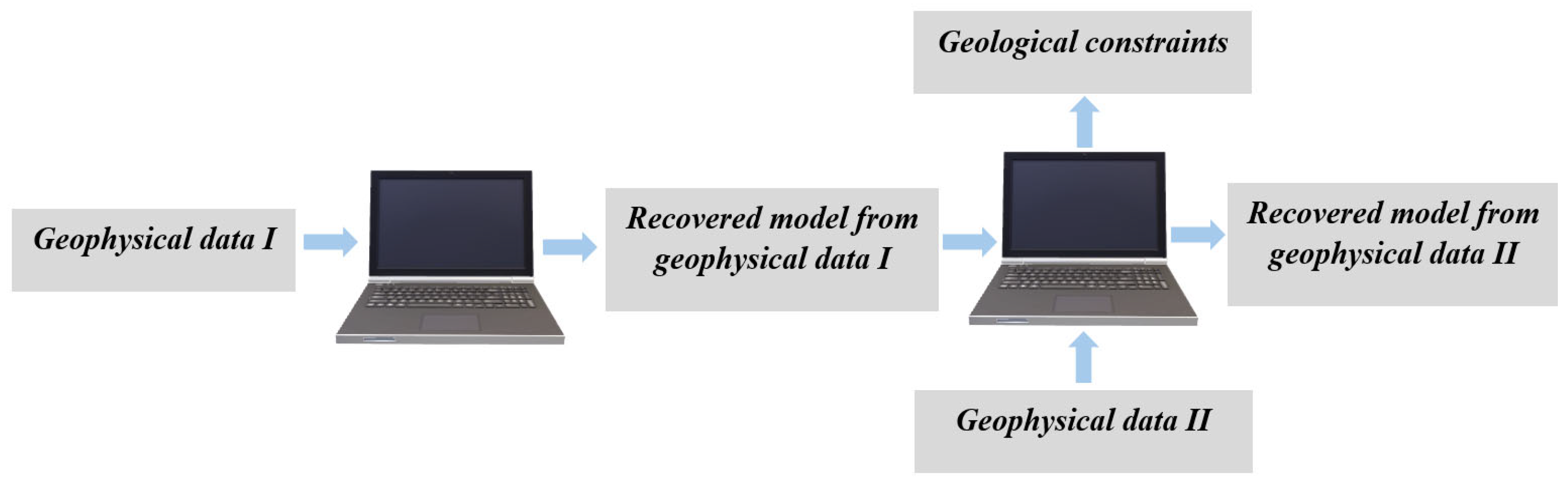
Figure 1. Illustration of sequential inversion of two arbitrary geophysical methods.
Remotesensing 18 01404 g001
Figure 2. (a) Schematic representation of a DC resistivity survey illustrating the injection of current (I) and the measurement of resulting electrical potential difference (DV) to determine apparent resistivity; (b) the dipole–dipole array configuration (modified from [24]), where r A and r B denote the distances from current electrodes A and B, while r M and r N represent the distances from potential electrodes M and N. r represents the position of a subsurface cell, a is the dipole spacing, and n a is the separation between the current and potential dipoles.
Remotesensing 18 01404 g002
Figure 3. (a) Fundamental principles of FDEM surveying illustrating the induction of eddy currents and the generation of the secondary magnetic field; (b) schematic representation of a typical FDEM survey geometry (modified from [24]), where r denotes the observation point (receiver location), r represents the subsurface cell position, r s corresponds to the source (transmitter) location, and S is the separation distance between the transmitter and receiver coils.
Remotesensing 18 01404 g003
Figure 4. Model parameters of the Synthetic Model I.
Remotesensing 18 01404 g004
Figure 5. Model parameters of the Synthetic Model II.
Remotesensing 18 01404 g005
Figure 6. Inverse resistivity models for Synthetic Model I: (a) separate inversion of EM34 data; (b) separate inversion of DC resistivity data; (c) cooperative joint inversion of EM34 data utilising DC resistivity as a prior constraint; and (d) cooperative joint inversion of DC resistivity data utilising EM34 as a prior constraint.
Remotesensing 18 01404 g006
Figure 7. RMS error convergence curves across iterations for separate and cooperative joint inversions (Synthetic Model I): (a) separate inversion of EM34 data; (b) separate inversion of DC resistivity data; (c) cooperative joint inversion of EM34 data utilising DC resistivity as a prior constraint; and (d) cooperative joint inversion of DC resistivity data utilising EM34 as a prior constraint The circular red markers indicate the specific iteration at which the algorithm satisfies the convergence threshold and terminates.
Remotesensing 18 01404 g007
Figure 8. Synthetic Model I pseudo-sections for the EM34 technique: (a) synthetic apparent resistivity data generated from the true model (refer to Figure 4), (b) calculated apparent resistivity response derived from the individual inversion model, and (c) calculated apparent resistivity response derived from the cooperative inversion model. The vertical and horizontal axes represent the pseudo-depth and profile distance (m), respectively, for the various T-R separations.
Remotesensing 18 01404 g008
Figure 9. Synthetic Model I pseudo-sections for the DC electrical resistivity technique: (a) synthetic apparent resistivity data generated from the true model (refer to Figure 4), (b) calculated apparent resistivity response derived from the individual inversion model, and (c) calculated apparent resistivity response from the cooperative inversion model. The vertical axis denotes the pseudo-depth (represented by the electrode spacing), and the horizontal axis represents the profile distance (m).
Remotesensing 18 01404 g009
Figure 10. Inverse resistivity models for Synthetic Model II: (a) separate inversion of EM34 data; (b) independent inversion of DC resistivity data; (c) cooperative joint inversions of EM34 data; and (d) cooperative joint inversion of DC resistivity data. The horizontal white dashed line represents the true boundary between the upper and lower geological layers, while the central vertical feature indicates the reconstructed dolerite dyke. The red frame highlights the location of the target dyke for visual comparison between the models.
Remotesensing 18 01404 g010
Figure 11. RMS error convergence curves across iterations for separate and cooperative joint inversions (Synthetic Model II): (a) separate inversion of EM34 data; (b) separate inversion of DC resistivity data; (c) cooperative joint inversion of EM34 data utilising DC resistivity as a prior constraint; and (d) cooperative joint inversion of DC resistivity data utilising EM34 as a prior constraint. The circular red markers indicate the specific iteration at which the algorithm satisfies the convergence threshold and terminates.
Remotesensing 18 01404 g011
Figure 12. Synthetic Model II pseudo-sections for the EM34 technique: (a) synthetic apparent resistivity data generated from the true model (refer to Figure 5), (b) calculated apparent resistivity response derived from the individual inversion model, and (c) calculated apparent resistivity response derived from the cooperative inversion model. The vertical and horizontal axes represent the pseudo-depth and profile distance (m), respectively, for the various T-R separations.
Remotesensing 18 01404 g012
Figure 13. Synthetic Model II pseudo-sections for the DC electrical resistivity technique: (a) synthetic apparent resistivity data generated from the true model (refer to Figure 5), (b) calculated apparent resistivity response derived from the individual inversion model, and (c) calculated apparent resistivity response from the cooperative inversion model. The vertical axis denotes the pseudo-depth (represented by the electrode spacing), and the horizontal axis represents the profile distance (m).
Remotesensing 18 01404 g013
Figure 14. Inverse resistivity models for the Morgenzon Farm field site: (a) separate inversion of EM34 data; (b) separate inversion of DC data; (c) cooperative inversion of EM34 data utilizing DC resistivity as a structural prior; and (d) cooperative inversion of DC resistivity data utilizing EM34 as a structural prior.
Remotesensing 18 01404 g014
Figure 15. Observed and calculated EM34 data for the Morgenzon Farm field site: (a) Measured field data of the EM34 approach; (b) calculated response from the individual inversion; and (c) calculated response from the cooperative inversion. The RMS misfit errors of computed data for separate and cooperative approaches are 2.35% and 1.27%, respectively.
Remotesensing 18 01404 g015
Figure 16. Observed and calculated DC resistivity data for the Morgenzon Farm field site: (a) Measured field data of the DC resistivity approach; (b) calculated response from the individual inversion; and (c) calculated response from the cooperative inversion. The RMS misfit errors of computed data for separate and cooperative approaches are 2.25% and 2.18%, respectively.
Remotesensing 18 01404 g016
Table 1. Comparative performance metrics for separate and cooperative inversions across synthetic benchmarks.
ModelTechniqueInversion MethodIteration NumberTime (s)RMSE (%)Target Reconstruction (%)
GeometryAmplitude
Model IEM34Separate7450.717888
Cooperative5720.738596
Electrical ResistivitySeparate6753.27785
Cooperative3923.258797
Model IIEM34Separate7363.257580
Cooperative6551.258495
Electrical ResistivitySeparate7492.277582
Cooperative7712.258895
Disclaimer/Publisher’s Note: The statements, opinions and data contained in all publications are solely those of the individual author(s) and contributor(s) and not of MDPI and/or the editor(s). MDPI and/or the editor(s) disclaim responsibility for any injury to people or property resulting from any ideas, methods, instructions or products referred to in the content.