Fully Automated Wind Site Assessment in Complex Terrain Using Satellite Data and Global Circulation Models

Highlights

What are the main findings?

• Data from Earth observation, global circulation models, and high-resolution fluid dynamics simulations are combined in an automated simulation workflow.
• The model accuracy challenges non-automated state-of-the-art simulation methods.

What are the implications of the main findings?

• The model is applicable globally with minimal manual input.
• De-risking investments might become feasible without costly on-site measurements.

Abstract

A globally applicable and fully automated simulation method based on satellite-derived Earth Observation (EO) data and global circulation models was developed and validated. Inputs to the simulation are DSM/DTM layers, surface roughness layer, forest canopy layer, and single-level point data from the European Centre for Medium-Range Weather Forecasts fifth-generation ECMWF reanalysis (ECMWF ERA5, a global circulation model produced by the Copernicus Climate Change Service (C3S)). High-resolution roughness length maps are produced by deep learning from optical satellite data. Velocity fields are predicted by fluid dynamics simulations in OpenFOAM using the IDDES turbulence model, a 3D resolved tree canopy implemented as isotropic momentum sinks, and a corrector step based on sub-grid-scale dynamic downscaling of ERA5 data. No calibration data from wind measurements close to the target are necessary to achieve results accurate enough for site assessments and wind park planning. The presented method is suitable for the prediction of average wind speeds and average power densities in complex terrain with high ruggedness indices for WEC (wind energy converter) installations closer to the ground and at hub heights of typical large-scale WECs.

1. Introduction

The focus of the research and development efforts was on automating simulations for applications in the wind industry and producing accurate predictions of wind speed in complex, rugged terrain with a non-uniform vegetation layer.

Automatically predicting physically correct wind speeds through Computational Fluid Dynamics (CFD) simulations in complex and rugged terrain has been an engineering challenge for decades. In wind resource planning the error in predicted wind power density is proportional to the third power of wind speed. Simulation validations using experimental data and blind comparisons are key to ensure highest accuracy results of wind speeds for a diverse set of input data.

Our approach does not use calibration loops for wind speed. The simulation workflow does not tune inlet wind speed profiles so that simulation results fit experimental data gathered in the simulated domain, often located close to the simulation target. This refers strictly to no use of local wind mast data to tune inlet conditions or model parameters for the specific site under study. The method yields average wind speeds and average power densities (and energy yields if the converter $c_p$ curve is known) in 3D space with high spatial resolution.

In the following sections, we describe the strengths and weaknesses of commonly used turbulence models in the wind industry. The newly developed workflow and models are validated with experimental wind data from two isolated hills. The established method is then applied to six different sites with wide-ranging terrain and vegetation complexity, and results are evaluated for different heights above ground level. Finally, we introduce a dynamic downscaling approach of global circulation model (GCM) wind data to correct wind speeds for unresolved topography in the GCM.

1.1. Related Work

The proposed end-to-end workflow for wind site assessment touches various scientific independent topics that are reviewed in this section. These are wind simulation, Digital Elevation Model generation, land cover classification, and surface roughness length derivation.

1.1.1. Wind Simulation Methods and Wind Site Assessment

A meta-analysis by Lee et al. [1] shows how the typical prediction bias of wind speed in the industry decreased over time from −16% in 2001 to around −3% in 2019. The accuracy requirement is underlined in [1] (p. 312), by citing Kline, stating: a change in 1% of wind speed can lead to 3% to 5% change in net present value. Barber et al. [2] conduct a simulation program comparison and try to find a compromise between cost and accuracy of different simulation methods (see Barber et al. [3]).

Go-to tools in preliminary site screening are publicly available wind power potential maps provided by the Global Wind Atlas (GWA) (see Badger et al. [4]) and the New European Wind Atlas (NEWA) (see Hahmann et al. [5], Dörenkämper et al. [6], Mann et al. [7]). From a pure efficiency standpoint, pre-calculated wind speed maps using meso-scale weather simulations as a generalization process for wind conditions, together with linearised Navier–Stokes flow models excel. Davis et al. [8] clearly state drawbacks of the wind atlases’ methods. GWA and NEWA work remarkably well in low-complexity terrain, but linearized models do not produce sufficiently accurate results in rugged orography (where the orography is sufficiently complex to cause an expected increase in bias and uncertainty due to the effect of overestimated speed-up effects due to the linearized flow model (Davis et al. [8], p. 14). The resolution and accuracy needed for bankable site assessments of complex wind farm sites exceed GWA and NEWA model capabilities, especially in mountainous regions. Also, small wind power installations that are often located closer to the ground or positioned in the vicinity of buildings, tree groups and forests cannot be accurately planned with publicly available wind atlases.

More capable models are therefore needed, and the wind industry intensively uses Reynolds averaged Navier–Stokes (RANS) models to overcome shortcomings of linearized Navier–Stokes models. RANS models offer better fidelity than linear models, are generally rather robust, and often the first step to more in-depth site evaluations. They also have their limitations. RANS-based solvers model turbulence locally and fail to correctly capture regions of detached flow and large-scale turbulence interactions. The economic value provided by RANS models is undoubtedly high with long ongoing efforts of tweaking semi-empirical model constants for specific use cases. Due to the affordability and ease of use compared to more advanced models, the wind industry at large clings to RANS despite the known problems and shortcomings (see Blocken et al. [9]). Efforts of said modification are documented exemplarily in Adbi et al. [10] that follow an automatic calibration approach.

Simulations of wind flow over medium-complexity terrain (Askervein hill) and high-complexity terrain (Bolund hill) were validated in this work (see below in Section 2.2.6). (validation of isolated model hills)). Askervein hill measurement campaign from 1983 (for documentation, see Taylor et al. [11] and Taylor et al. [12]) still mattered as a reference for state-of-the-art wind simulations in the late 1990s (see Gravdahl et al. [13]). DTU’s benchmark hill Bolund enters the picture almost three decades after the Askervein experiment—at a time when the limitations of RANS turbulence closure models already show their limitations for complex cases and pure Large Eddy Simulation (LES) and hybrid Detached Eddy Simulation (DES) (see Spalart [14], Spalart et al. [15]) for realistically high Reynolds numbers started becoming economically feasible in wind engineering. Exponentially increasing computational power and newly developed turbulence model capabilities enabled high-fidelity simulations of wind flow over abruptly changing topographies.

The Bolund hill campaign conducted experiments and blind simulation tests. Some sobering results from the blind test and following advances reverberated in industry and academia for a decade (see Bechmann et al. [16,17,18], Berg et al. [19], Diebold et al. [20], Yeow et al. [21,22], Lange et al. [23], Cuerva-Tejero et al. [24], Chaudari et al. [25], Vladut et al. [26]). With increasingly available high-resolution wind tunnel measurements and real-world experimental data, the simulation accuracy and the shortcomings of linear and RANS models became even more obvious.

For over six decades, LES had its place in Atmospheric Boundary Layer (ABL) research (Stoll et al. [27]) and DES is used routinely in the wind industry for de-risking larger investments (see Hristov [28]). The dichotomy of “real” and synthesized inlet turbulence (see Poletto et al. [29]) is not solved yet. Synthetic turbulence generators offer great potential for reduction in computational effort with the downside of having to know the in-flow velocity spectra in advance. Big savings in compute time in some cases can also be achieved by switching to lower accuracy floating point arithmetics (see Lysenko [30]) with technically negligible effects to the fidelity of simulation results. As always, the acceptable simplifications depend on the use case. Important topics and relevant as ever in simulation pre-processing are the effects of simulation/experimental domain sizes (see Wang et al. [31]) and specifics in boundary layer mesh generation (see Gargallo et al. [32]).

All of the knowledge and methods described above went into the design of the presented simulation method. Our approach has its own strengths and weaknesses. The limits of the model and workflow applicability are explained below.

Wind simulation needs as input a high-resolution representation of Earth’s topography and very high-resolution roughness length data of all objects on top of it. A common way to describe topography is the use of Digital Elevation Models (DEMs). The surface roughness length can be derived in various ways from remote sensing data. In this paper, we focus on methods that derive the roughness length from Land Use and Land Cover (LULC) classifications and from the so-called normalized digital surface models (nDSMs).

1.1.2. Comparison with Other Frameworks and Commercial Wind Simulation Software

In this section, we show how our method differs from established workflows in the wind industry. Prominent and market-dominating wind simulation expert systems include WAsP-2025-B-04 (developed by DTU), MeteoDyn 1.5.0.0 and Windsim 12.25 (owned by CLS group), WindPro 4.2 (by EMD International) and Wind Farmer 1.6.5.1 (by DNV). WAsP uses linear models extensively and offers a CFD option for complex terrain that is RANS only (no LES). MeteoDyn WT, used for wind farm planning, offers mesoscale coupling and CFD by default and is able to tune simulation data with its Multi-mast tool, basically calibrating simulation results with measurement data within the domain. WindPro uses either WAsP’s CFD code or OFWind based on OpenFOAM-2.3.x (both RANS) as simulation backend. Wind Farmer uses STAR-CCM+ 2510, a commercial CFD package, as solver and applies local calibration methods for increased simulation accuracy. Our method differentiates itself from established tool chains by using no local calibration data of wind speed and running simulations with a LES model by default. This aims for reliable and calibration-free simulations in terrain with high ruggedness indices.

1.1.3. Digital Elevation Model Generation from Remote Sensing Data

DEM generation from remote sensing data at a regional to global scale encompasses multiple methodological approaches, each with distinct data acquisition principles, processing workflows, and accuracy characteristics. Recent literature emphasizes three primary technological domains: optical photogrammetry, interferometric synthetic aperture radar (InSAR), and light detection and ranging (LiDAR), alongside emerging deep learning-based enhancement techniques.

Stereo image acquisition from overlapping orbital passes enables dense stereo matching algorithms (predominantly Semi-Global Matching in Hirschmüller et al. [33] and Pyramid Stereo Matching Network in Chang et al. [34]) to establish pixel correspondences, followed by triangulation to derive three-dimensional coordinates. Current studies show that vertical accuracies with respect to LiDAR references data are achievable with twice the ground sampling distance (GSD) for the normalized median absolute deviation or 10 times the GSD for the root mean square error (RMSE). Details are given in Perko et al. [35] for the Pléiades constellation, in Wang et al. [36] for WorldView-2, and in Du et al. [37] for Gaofen-7.

InSAR-based DEM generation exploits phase difference measurements between two spatially separated SAR acquisitions, requiring co-registration, interferogram formation, coherence estimation, adaptive filtering, phase unwrapping, and phase-to-elevation conversion. Operational systems including SRTM (30 m), TanDEM-X (12 m), and Sentinel-1 (~10 m) achieve vertical accuracies of approximately 16 m (SRTM, in Rabus et al. [38]), at least 10 m (Tandem-X, in Wessel et al. [39]) and in the order of 40 m (Sentinel-1, in Zhang et al. [40]), with particular advantages in cloud-prone regions though accuracy degrades in low-coherence areas such as dense vegetation as in Wessel et al. [39], in Rodriguez et al. [41], and in Braun [42]. For Sentinel-1, a very recent study report high accuracy for the 1-day pair (RMSE ≈ 14.7 m) with moderate degradation for the 6-day pair (RMSE ≈ 16.4 m), but a pronounced loss of accuracy for the 12-day pair (RMSE ≈ 49.4 m) as in Braun [42].

Airborne LiDAR provides centimeter to sub-meter vertical precision through active laser scanning yielding dense point clouds (4–20 points/m²) that require classification into ground and non-ground returns via progressive densification algorithms or Cloth Simulation Filters before DEM interpolation; see Lakshmi et al. [43], Chandra et al. [44], Tian et al. [45], and Liu et al. [46]. Recent deep learning denoising innovations, such as the DEN4 algorithm, achieve 70.2% mean square error reduction and 37.8% signal-to-noise ratio improvement compared to traditional filtering methods as in Lu et al. [47].

Emerging convolutional neural network architectures address DEM super-resolution through ensemble learning frameworks incorporating geographical terrain zoning and multi-network integration, demonstrating 2.8% accuracy improvements over the baseline method in Dong et al. [48]. Multi-source fusion approaches combining low-resolution elevation data, namely Shuttle Radar Topography Mission (SRTM) with higher-resolution multi-spectral imagery (Sentinel-2) through residual channel attention networks, enable fine-scale topographic reconstruction in data-scarce regions in Han et al. [49] and in Zhu et al. [50].

The globally available dataset Forests and Buildings removed Digital Elevation Model (FABDEM, see Hawker et al. [51]) is a global 30 m resolution DTM that removes elevation biases from forests and buildings in the global 30 m resolution version of the Copernicus Digital Elevation Model using machine learning. In particular, Random Forest algorithms were trained on reference datasets like LiDAR from 12 countries to correct elevation biases caused by forests and buildings. Validation shows substantial improvements over the original global 30 m resolution version of the Copernicus Digital Elevation Model, reducing the mean absolute error from 5.15 to 2.88 m in forests and from 1.61 m to 1.12 m in built-up areas.

A nDSM represents the vertical elevation of anthropogenic and natural features, including buildings, infrastructure, and vegetation, expressed relative to the underlying bare-earth terrain surface represented by a DTM. The mathematical relationship is expressed as $\mathrm{nDSM}=\mathrm{DSM}-\mathrm{DTM}$, where the DSM captures the topmost exposed surface, including all objects and vegetation canopy, while the DTM represents the bare ground or terrain surface devoid of such features. This normalization procedure yields elevation values ranging from zero at ground level to the maximum height of the tallest features, enabling direct comparison of feature heights independent of underlying terrain slope and elevation. The primary methodological approach for nDSM derivation involves subtraction of a reference DTM from remotely sensed DSM data, where DTMs are conventionally derived from airborne laser scanning (ALS) campaigns using hierarchic robust filtering techniques to classify laser echoes into terrain and off-terrain points, with final DTM computation typically based on the last-pulse return information, which penetrates vegetation canopy to reach the ground surface in Baltsavias [52]. Where ALS data are unavailable at global or regional scales, alternative approaches employ morphological filtering algorithms and ground point classification methods applied directly to DSM point clouds to extract underlying terrain information without explicit DTM reference, enabling nDSM estimation from satellite-derived DSM through digital filtering and elevation surface refinement procedures in Meng et al. [53] and in Perko et al. [54]. The nDSM product serves critical applications, including building height estimation and urban structure characterization, tree canopy height modeling for forestry and biomass assessment, detection of single-tree locations in dense forest environments, above-ground vegetation structure analysis, and multi-temporal change monitoring of landscape features. Quality assessment of derived nDSMs depends substantially on both source data resolution and the accuracy of underlying DTM reference data, with standard errors typically ranging from centimeter-scale precision in ALS-derived products to meter-scale uncertainty in filtering-based approaches applied to coarser satellite DSMs; see Wagner et al. [55], Fissore et al. [56], Hyyppa et al. [57], Leopold et al. [58], and Wu et al. [59].

1.1.4. Land Cover Classification from Remote Sensing Data

LULC classification from remote sensing data constitutes a fundamental analytical technique for environmental monitoring, spatial planning, and sustainable resource management. Recent literature demonstrates a methodological evolution from traditional statistical approaches toward deep learning architectures, with concurrent advances in global operational products leveraging multi-sensor satellite constellations. The term LULC is often used to refer specifically to land cover, as satellites directly observe physical surface features. Land use is typically inferred from these observations, effectively making land cover a proxy for land use; see Mustafic et al. [60].

Maximum Likelihood Classification (MLC) and Support Vector Machine (SVM) represent established parametric and non-parametric methods, achieving overall accuracies of 70.60–84.17% on Sentinel-2 imagery in Topalouglu et al. [61]. SVM demonstrates superior generalization across diverse datasets, with kernel variations (linear, radial basis function, polynomial, sigmoid) consistently achieving 88–99.17% accuracy depending on data complexity and training sample quality in Arsiso [62]. Random Forest (RF), an ensemble decision tree classifier, exhibits robust performance in heterogeneous landscapes, attaining 86.56–99.36% overall accuracy with Kappa coefficients exceeding 0.99. RF’s computational efficiency with high-dimensional data and resistance to overfitting make it particularly suitable for multi-spectral and multi-temporal remote sensing applications; see Ojwang et al. [63], Baheer et al. [64], and Gaw et al. [65].

Convolutional Neural Networks (CNNs) eliminate manual feature engineering through hierarchical automatic feature extraction, achieving 96–98.74% overall accuracy on benchmark datasets. Pre-trained architectures including very deep convolutional networks from the Visual Geometry Group in Oxford (VGG, especially VGG16, VGG19), Residual Network (ResNet, especially ResNet50, ResNet152), and EfficientNet demonstrate exceptional performance when fine-tuned via transfer learning on domain-specific LULC datasets. Chaurasia et al. [66] reported VGG19 as optimal for Indian urban contexts, achieving 96% accuracy with superior computational efficiency compared to deeper ResNet architectures (see Zhao et al. [67], Dastour et al. [68], and Mustafic et al. [60]). Transformer-based models incorporating attention mechanisms represent emerging paradigms, with Khan et al. [69] demonstrating 49 million trainable parameters enabling advanced contextual learning for complex satellite imagery classification.

Zhao et al. [67], in a comprehensive review with 99 citations, systematically analyzed deep learning frameworks for LULC classification, concluding that CNNs, Fully Convolutional Networks (FCNs), and transfer learning approaches substantially outperform traditional machine learning methods. However, methodological selection depends on data availability, computational resources, and application requirements, with Random Forest remaining competitive for operational applications requiring interpretability and computational efficiency, see Khan et al. [70], Mustafic et al. [60], and Charasia et al. [66].

1.1.5. Surface Roughness Length Derivation from Land Cover Classification

Aerodynamic roughness length ($z_0$) represents the height at which wind speed theoretically approaches zero in the logarithmic wind profile, constituting a fundamental parameter for characterizing land surface-atmosphere momentum, energy, and mass exchange. The derivation of $z_0$ from LULC classification has evolved from simple lookup table approaches toward sophisticated machine learning and remote sensing integration methodologies.

Ramli et al. [71] demonstrated that $z_0$ can be estimated from Normalized Difference Vegetation Index (NDVI) through exponential relationships of the form

$$z_0(x,y)=\exp (c_1+c_2·\mathrm{NDVI}),$$

(1)

achieving $r^2=0.86$ correlation with Davenport Terrain Classification when calibrated using Landsat Thematic Mapper data in Wilford et al. [72]. This semi-empirical approach combines quantitative remote sensing information with qualitative land cover classification to enable spatially distributed roughness characterization.

Hu et al. [73], representing the first study demonstrating machine learning for highly accurate surface roughness estimation with 39 citations, trained ensemble algorithms on FLUXNET—see Pastorello et al. [74]—eddy covariance observations using predictors including vegetation indices, leaf area index, canopy height, and climate variables to derive $z_0$ values that substantially improved surface turbulent flux estimates. Wang et al. [75] developed a Random Forest Regression framework combining ERA5 reanalysis with China Meteorological Administration station observations to generate high-resolution monthly gridded $z_0$ datasets, achieving 89.9% reduction in Weather Research and Forecasting (WRF) model 10 m wind speed errors over built-up areas compared to default parameterizations.

1.2. Research Gap and Contribution

In this work, we outline the unit operations and inner workings of a novel expert system for simulation of wind conditions in complex terrain, incorporating Earth Observation data with the goals to produce sufficiently accurate, cost-effective and reliable results. After extensive research, it was concluded that no known (commercial) software system with an automated workflow applicable at the highest ruggedness indices and terrain complexity that fulfills the above goals exists. The most demanding simulations seem to be handled case by case at large-scale wind energy planners and engineering companies. Our method combines

1.

well-known, tested, and trusted transient turbulence models with

2.

globally available weather data and

3.

surface models based on earth observation data

• based on

4.

identification of suitable remote sensing data, to derive key parameters for modeling,

5.

generation of LULC classification, and

6.

automated workflow for CFD preprocessing.

The combination of all the mentioned aspects in a single system without the use of calibration techniques is our contribution to this field of research.

1.3. Outline

This paper is organized as follows: Section 2 describes the materials and methods, including detailed information about the test sites, data, and the methodologies proposed in this work. Section 3 presents the results, followed by a discussion of the key insights in Section 4. Finally, Section 5 draws conclusions from the study.

2. Materials and Methods

To allow sophisticated evaluation, six test sites were selected in the United States and Europe. Section 2.1 describes all materials used, in particular the test sites and according data. Section 2.2 discusses our algorithmic approaches beyond state of the art with respect to workflow design, surface models based on earth observation data, and automated workflow for CFD pre-processing. For flow simulation, we use a combination of sector-wise, high-resolution, transient simulations and dynamic downscaling of weather data on a coarser mesh. The dynamic downscaling approach enables input data correction of wind speeds in mountainous regions. CFD meshes are created from DSM/DTM data and local surface roughness is mapped to ground facets of the generated mesh. Surface roughness and vegetation cover are generated by machine learning methods from RS data.

2.1. Materials

This Section describes the input data used in the project. It is divided into Section 2.1.1 addressing Remote Sensing Data and Section 2.1.2 describing the ECMWF ERA5 data, high-resolution reanalysis data from the European Centre of Medium-Range Weather Forecasts. Section 2.1.3 addresses experimental data from wind mast measurements and production data from a large-scale wind turbine to evaluate the simulated results.

2.1.1. Remote Sensing Data: DSMs, Orthoimages, Canopy Height Models

Globally, elevation data were sourced from the global 30-m resolution version of the Copernicus Digital Elevation Model (hereafter referred to as CopDEM-30 or Copernicus DEM), a worldwide Digital Surface Model (DSM) representing the Earth’s surface, including buildings, infrastructure, and vegetation at 30 m spatial resolution (1.0 arc second grid spacing). The CopDEM-30 is derived from the edited WorldDEM™ product (Immenstaad, Germany), which itself originates from bistatic X-band Synthetic Aperture Radar (SAR) data acquired during the TanDEM-X Mission between December 2010 and January 2015, a Public–Private Partnership between the German Aerospace Centre and Airbus Defence and Space. Post-processing enhancements applied to WorldDEM include hydrological editing such as flattening of water bodies and enforcement of consistent river flow networks, geometric editing of shorelines and coastlines, refinement of special features including airports, and correction of implausible terrain structures. Data voids in the TanDEM-X coverage were filled using auxiliary elevation sources, including ASTER GDEM, SRTM (30 m and 90 m), GMTED2010, ALOS World 3D-30m, TerraSAR-X radargrammetric DEM, and select national DEMs (Norway, Spain). The Copernicus DEM employs the WGS84-G1150 horizontal datum (EPSG:4326) and EGM2008 geoid vertical reference (EPSG:3855), with elevation values expressed in meters. Independent validation indicates absolute vertical accuracy of <4 m at 90% linear error, with global mean accuracy of 1.92 m (excluding Antarctica and Greenland) validated against ICESat GLAS reference points, and relative vertical accuracy of <2 m for slopes ≤20% and <4 m for slopes >20%. Recent comparative assessments demonstrate that CopDEM-30 achieves superior vertical accuracy compared to alternative freely available global DEMs, including NASADEM, SRTM, and ASTER GDEM across diverse terrain types, see the product handbook [76] and Meadows et al. [77].

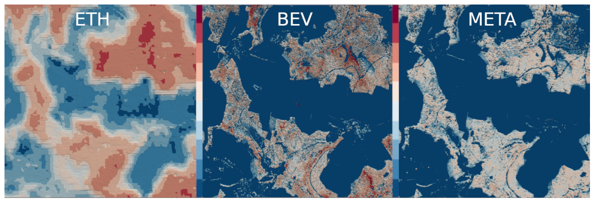
In addition to high accuracy in forested areas, we also strived to achieve global elevation data coverage, including tree canopy models. Recently, the globally available dataset Forests and Buildings removed Digital Elevation Model (FABDEM, see Hawker et al. [51]) was published. FABDEM is based on Copernicus Digital Elevation Model (CopDEM, see product handbook [76]) at 30 m lateral resolution and employs machine learning to generate and subtract canopy/building heights and so removes artifacts from forests and buildings in Copernicus DEM (also see Ledoux et al. [78]). Shortly after the publication, a comparable global canopy dataset was released by ETH Zürich (Lang et al. [79]). Another year, later META’s canopy model featuring below 1 m lateral resolution and global availability was published under a permissive licence (Tolan et al. [80]).

For global nDSM representation, this study employed the Meta Canopy Height Model in Tolan et al. [80], a high-resolution global dataset providing tree canopy height estimates at 1 m spatial resolution across Earth’s terrestrial surface. Developed through collaboration between Meta’s Fundamental AI Research and Sustainability teams and the World Resources Institute (WRI), the dataset was generated using self-supervised vision transformer architectures combined with convolutional decoders trained on aerial LiDAR reference data. The underlying approach leverages DINOv2 in Oquab et al. [81] for feature extraction from approximately 18 million RGB satellite images, followed by Dense Prediction Transformer in Ranftl et al. [82] decoding to generate pixel-wise canopy height predictions. Input imagery was sourced from Maxar’s Vivid mosaic basemap at 0.5 m resolution, spanning the acquisition period 2009–2020, with 80% of the data derived from imagery captured between 2018 and 2020. The model training procedure consisted of two phases: (1) self-supervised pre-training on the global Maxar imagery corpus to generate universal feature encodings and (2) supervised fine-tuning of the convolutional decoder against aerial LiDAR canopy height maps from the United States, supplemented by post-processing calibration using Global Ecosystem Dynamics Investigation spaceborne LiDAR observations to ensure global consistency (Dubayah et al. [83]). Independent validation against withheld aerial LiDAR reference data demonstrates a Mean Absolute Error of 2.8 m and Mean Error of 0.6 m for canopy height prediction. Both the global canopy height dataset and the trained AI model are publicly available under Creative Commons Attribution 4.0 International License via Google Earth Engine and Amazon Web Services platforms, enabling reproducible forest monitoring, carbon stock assessment, and restoration verification applications.

For Austrian test sites, elevation and imaging data were sourced from the authoritative geospatial dataset repository maintained by Austria’s Federal Office of Metrology and Surveying (Bundesamt für Eich- und Vermessungswesen, hereafter referred to as BEV), a federal authority established in 1923 and responsible for collecting, maintaining, and distributing national base geodata constituting the foundation of Austria’s spatial data infrastructure. Specifically, this study utilized orthoimagery acquired from airborne photographic campaigns conducted by the BEV with a ground sampling distance of 0.2 m, processed into geometrically corrected orthophotos with sub-meter spatial resolution and comprehensive nationwide coverage. Additionally, airborne laser scanning (ALS)-derived DSMs and DTMs from the BEV’s comprehensive national ALS coverage were employed, both provided at 1 m spatial resolution representing the Earth’s bare-ground surface and the top-of-canopy/building surface, respectively. The high-resolution DSM and DTM datasets from the BEV represent a cooperative product of Austrian federal and state-level geodata providers, acquired through standardized ALS survey campaigns employing contemporary laser scanning technology with consistent geometric and radiometric calibration across the entire territory. For the Austrian test sites evaluated in this study, nDSM derivation was executed straightforwardly through direct subtraction of the coincident 1 m resolution DTM from the corresponding DSM (nDSM = DSM − DTM), yielding height above-ground values for all buildings, infrastructure, and vegetation throughout the study domains. Throughout this manuscript, this comprehensive Austrian dataset collection is referenced collectively as “BEV data”. The availability of high-quality, spatially consistent ALS-derived reference elevation data from BEV substantially facilitated independent validation of derived topographic parameters and improved the confidence of nDSM calculations at the Austrian test sites compared to the methodology required for global assessments lacking such authoritative elevation products as the ones from Federal Office of Metrology and Surveying [84] and Kakoulaki et al. [85].

Moreover, ESA World Cover 2022 [86], a global land cover map produced by the European Space Agency for the year 2021 with a 10 m resolution, was used. It used Sentinel-1 and Sentinel-2 satellite data, developed under the ESA WorldCover project. The map covers the entire Earth’s surface with 11 standardized classes (including tree cover, shrubland, grassland, cropland, built-up areas, bar/sparse vegetation, snow/ice, permanent water bodies, herbaceous wetland, mangroves and moss/lichen) based on the United Nations Food and Agriculture Organization Land Cover Classification System, enabling consistent global comparisons. The map is freely available under Creative Commons Attribution 4.0, delivered as Cloud-Optimized GeoTiFFs in 3 × 3-degree grid (EPSG:4326, WGS84), totaling approximately 120 GB, which each tile including a primary map layer and an auxiliary quality layer indicating Sentinel data reliability. Independent validation by Wageningen University and International Institute for Applied Systems Analysis reports an overall accuracy of $76.7\pm 0.5\%$ with detailed metrics in the Product Validation Report. It is openly available under ESA World Cover [86].

For generating the very high-resolution LULC data, both airborne data and ESA’s WorldCover2022 product were utilized. In Austria, we used BEV data to obtain the LULC, in other parts the ESA World Cover 2022 has been used. Data preparation involved downloading the relevant tiles from the ESA WorldCover viewer ([86,87]), reprojecting them to the target map projection, stitching tiles where necessary, and performing gap filling.

2.1.2. Global Weather Data: ECMWF ERA5

Global atmospheric reanalysis data were sourced from ERA5, the fifth-generation European Centre for Medium-Range Weather Forecasts (ECMWF) atmospheric reanalysis of the global climate covering the period from January 1940 to present, produced operationally by the Copernicus Climate Change Service (C3S). ERA5 provides hourly estimates of a comprehensive array of atmospheric, land-surface, and oceanic climate variables at approximately 31-kilometer horizontal grid spacing (0.28° × 0.28° reduced Gaussian grid, N320) and resolves the atmosphere using 137 vertical levels from the Earth’s surface up to a height of 80 km (approximately 1 Pa top-of-model pressure). The reanalysis is based on the Integrated Forecasting System (IFS) Cycle 41 Release 2 (Cy41r2), which incorporates a decade of subsequent development in model physics, atmospheric dynamics, and data assimilation methodologies compared to its predecessor ERA-Interim. ERA5 integrates vast quantities of historical in situ and satellite observations into global fields using advanced four-dimensional variational (4D-Var) data assimilation with a 12 h assimilation window, providing complete spatial and temporal coverage without data gaps. The reanalysis incorporates uncertainty quantification through a 10-member ensemble data assimilation system at half the horizontal resolution (63 km) and reduced temporal resolution (3-hourly), enabling assessment of synoptic and analysis uncertainty across all variables. ERA5 provides a substantially improved representation of historical atmospheric circulation patterns, the global hydrological cycle, and surface energy budgets compared to ERA-Interim, and benefits from assimilation of numerous reprocessed satellite data records, including instruments such as IASI, ASCAT, CrIS, MWHS-2, TMI, SSMIS, and AMSR-2. Following the cessation of ERA-Interim production on 31 August 2019, ERA5 has become the authoritative global atmospheric reanalysis product for climate and weather applications, with operational updates maintained with a latency of approximately 5 days and ongoing coverage extending to the present date. Detailed technical specifications, validation assessments, and access to all ERA5 data products are available through the Copernicus Climate Data Store (https://cds.climate.copernicus.eu, accessed on 20 February 2026) and comprehensive documentation through the ECMWF Confluence Knowledge Centre (https://confluence.ecmwf.int, accessed on 12 February 2026); see Hersbach et al. [88], Soci et al. [89], and Hersbach et al. [90].

In our workflow, ERA5 data are interpolated bilinear from the four nearest grid neighbor points of the target site before further processing. Primary inputs for the wind simulations are sector-wise (usually 16), mean values of u,v point data of wind speeds on ERA5 model level 137 from the last 10 years. If experimental data were time-limited, we used only full years of ERA5 data that covered measuring periods. For dynamic downscaling, we used hourly u,v point data of wind speed on ERA5 model level 137 directly as linear time-interpolated, transient boundary conditions.

2.1.3. Reference Wind Data

For experimental wind speeds of isolated hills, we used data from the detailed measurement campaigns of Askervein and Bolund (see Section 1.1). For North American sites, we relied on data provided by the National Ecological Observatory Network (NEON) and Tall Tower Dataset via the Bonneville Power Administration. Long-term measurement data for Austrian sites were kindly provided by our project partners FH Technikum Wien (ARGE Lichtenegg) and Energie Steiermark AG, Graz, Austria. See

Table 1. Summary of validation site locations and number of simulated wind directions (sectors).

Ref.	Site Name (Exp. Data Provider), State	Latitude [°]	Longitude [°]	Sim. Sectors
1	Naselle Ridge (tall tower dataset), USA	46.4220	−123.7983	1 (NW)
2	Megler (tall tower dataset), USA	46.2660	−123.8774	1 (S)
3	Mtn. Lake Biological Station (NEON), USA	37.3783	−80.5248	1 (WNW)
4	Soaproot Saddle (NEON), USA	37.0334	−119.2622	1 (S)
5	Handalm wind park (E-Stmk), AT	46.8507	15.0080	16 (all)
6	Lichtenegg research wind park (FHTW), AT	47.6089	16.2035	16 (all)

for validation site locations and the number of simulated wind directions (sectors).

2.2. Methods Overview

In the following Section 2.2.1, a detailed description of the automated wind simulation and its sub-modules and functions is given. Section 2.2.2 describes the preparation of the raster datasets. Section 2.2.3 addresses the parametric generation of the surface geometry on which the CFD simulations are run. Apart from the surface, vegetation layers and buildings are essential for modeling wind speeds. We put a special focus on the vegetation layer, which can strongly influence the production of small wind power plants (see Section 2.2.4). Section 2.2.5 deals with input data generation for wind from global circulation models and dynamic downscaling. Section 2.2.6 explains how we validated turbulence models and workflows against experimental data from detailed measurement campaigns of two well-documented isolated model hills.

2.2.1. Workflow

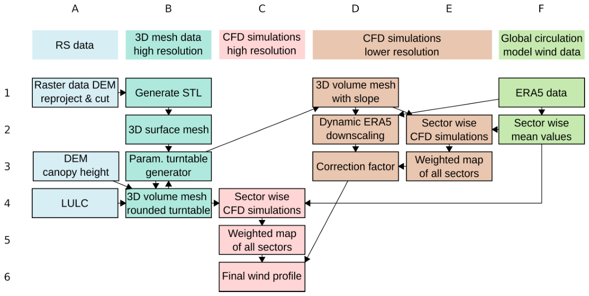
The following Figure 1 gives an overview of the modules and data flows involved in the automatic wind simulation. Columns are colored by data type/domain. Rows show (sorted chronologically from top to bottom) the approximate order of sub-processes. Arrows indicate data flow and dependencies. The complete workflow is implemented via a batch processing system on a high-performance computing system. The batch processing system manages sub-process dependencies, job ordering, and maximizes overall system usage. The sub-modules are referenced by their coordinates (see Figure 1), e.g., F1 for “ERA5 data”.

The only mandatory inputs for simulations are latitude, longitude, and hub height of the target. Based on the geo-coordinates, terrain data are generated with remote sensing-based paradigms (column A) and wind data are queried (column F). Apart from the three input variables, no further user interaction is necessary. In case the user needs non-default settings or more granular control, all modifiable parameters are exposed in configuration files for geometry generation, solver control, and post-processing.

2.2.2. Implementation

The preparation of the raster datasets, including the DEM and the Canopy Height Model (CHM) (Figure 1, A1 and A3), comprised the reprojection of the respective input data to the defined target coordinate system, mosaicking of input tiles where necessary, and clipping to the designated output frames (i.e., 10 × 10 km² and 2 × 2 km²) centered on the target coordinates. Subsequently, the data sampling was harmonized to spatial resolutions of 30 × 30 m² for the larger frame and 2 × 2 m² for the inner frame, respectively. Finally, the Terrain Ruggedness Index (TRI) was computed based on the processed DEM. For test sites outside Austria, we used the same procedure as described above to prepare the ESA Worldcover as input LULC. For the Austrian test sites, the BEV orthophotos were preprocessed analogously to the procedure described above, and the LULC classification (Figure 1, A4) was derived according to the methodology outlined in Section 2.2.4. Those land cover classifications are recoded into roughness length data following the method described in Floors et al. [91]. All processing steps were conducted using a script implemented in the proprietary scripting language of the in-house software Remote Sensing Software Graz (RSG), thereby exploiting the corresponding built-in functionalities for data processing and analysis; see Perko et al. [35] and Perko [92].

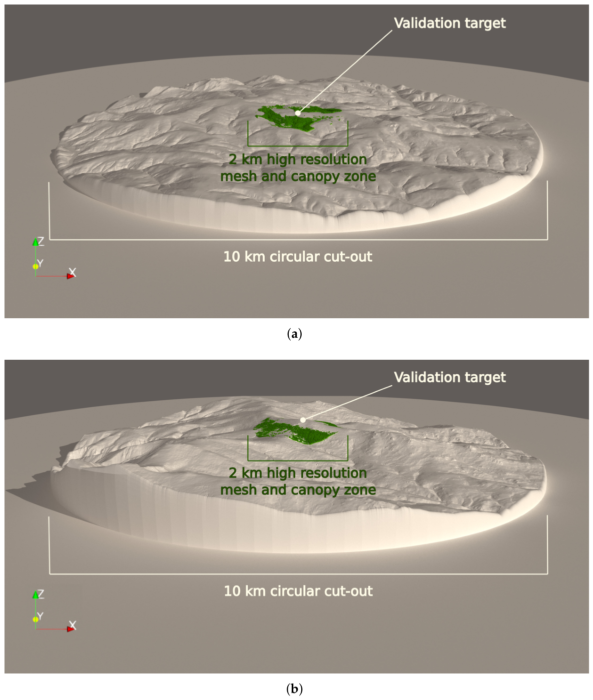
Reprojected, stitched, and cropped raster data (defaults to 10 × 10 km²) are converted to x, y, z data and ingested by a parametrised 3D modeler that generates a surface mesh with local grid refinement dependent on slope changes. The surface mesh is parametrically transformed to a turntable style geometry (for visualization, see Figure 2). The turntable geometry with a flat (i.e., horizontal) bottom at the side and inlet boundaries is the basis for a hex-dominant 3D finite volume mesh with boundary layer and central zone refinements. Surface roughness lengths obtained by raster data input are mapped to the turntable and a 3D resolved forest zone is generated in the central refinement zone (defaults to 2 km in diameter). See Column B in Figure 1.

Separate finite volume meshes are created for each simulated incoming wind direction (sector). Transient simulations are run until a pseudo-equilibrium flow state is reached, ensemble averaged for an additional interval of 600 s of flow time and weighted by frequency of incoming sector occurrence to yield yearly average values. See Column C in Figure 1.

Simultaneously, a coarser and wider (25 × 25 km²) 3D volume mesh with 100 m lateral resolution and gentle sloping inlet is created for a dynamic downscaling simulation using ERA5 hourly values (see Column F Figure 1) set at the vertical domain boundaries. Additionally, each sector is simulated with the coarser mesh resolution and gentle inlet slope to derive a local correction factor—i.e., the ratio of average wind speeds at the target for a long-term mean value inlet to the average wind speed at the target for dynamic inlets. Those extra steps in Columns D and E (see Figure 1) are necessary to correct for the wind conditions that were filtered out by sector-wise averages.

2.2.3. Geometry Generation

In Figure 2, surface meshes generated from raster data input (from BEV ALS DTM layer tiles [84]) for Lichtenegg and Handalm validation sites are shown. The circular cut-out is placed on a flat plane that is located at the lowest height within the cut-out geometry. A wind-tunnel-like flow box is created around the circular cut-out with sufficient space above the terrain to minimise compression effects and unphysical speed-up of the in-flow profile. For each simulated sector, a separate hex-dominant finite volume mesh is created to ensure that most cells are orthogonal to the planar in-flow, side, and top boundaries. This minimizes numerical correction steps, reduces total simulation run-time, and enhances solver stability.

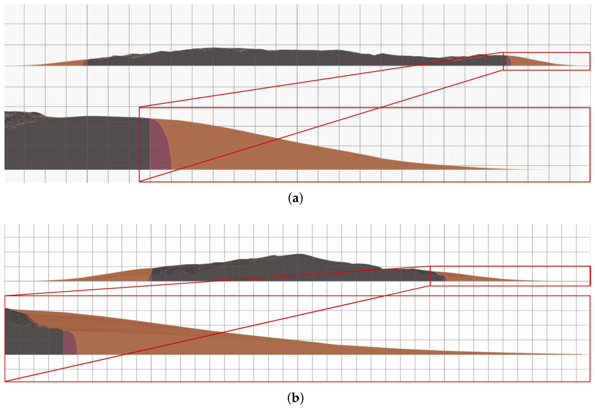
Parametric geometry creation from raster data currently automatically creates several surface shapes defined by preset parameters: a straight circular cut, rounded edges of the outer cut and a parametric, adaptive slope modeled after Askervein hill. The rounded edge type is the standard model, showing the best compromise of domain size, calculation time, and simulation error. The slope geometry is used in dynamic downscaling simulations and ensures correct wind speed-ups for lower mesh resolutions (see Figure 3).

2.2.4. Key Parameters for Wind Modeling Above Terrain Surface

Requirements of the developed model were accurate predictions of wind speeds close to the ground for small wind power applications, as well as higher up wind speeds at typical hub heights for large wind energy converters (WECs). Our current focus of key parameters here is limited to forests, since the use case primarily concerns mountainous regions where other key parameters as buildings do not occur. Sogachev et al. [93] clearly point out the limitations of a pure roughness patch approach for modeling wind speeds close to the ground, at locations near forest edges or in cases of short catches over small and inhomogeneous forest areas. We were able to reproduce the model behaviors and findings of Sogachev et al. Resolved tree canopy models can be derived from single tree studies (see Mochida et al. [94] and Poh et al. [95]) but derived resistance parameters are only valid for single trees, tree groups, and dense hedges. Cedell [96] gives the most valuable insights into how the wind engineering industry deals with larger forested areas under increasing accuracy requirements. Liu et al. [97] completed the picture of a methodology that highly resembles the one developed and validated in this research project.

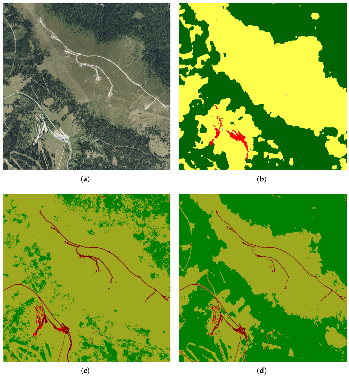
Based on Mustafic et al. [60], AI methods are used to obtain LULC maps for all Austrian test sites. The obtained LULC maps have as output five to ten different classes (i.e., forest, herbaceous, water surface, building, etc.). A deeper analysis of the first results showed issues in the model quality, as the model was trained for different sensors, flying heights and imaging nodes and therefore was only partially able to compensate such radiometric variations. To improve the model’s quality additional datasets, especially further BEV data, acquired in different years, seasons and under varying sensor configurations and flight settings, were used to re-train the model. The improvements on the model’s quality are demonstrated in Figure 4 for the test site Handalm.

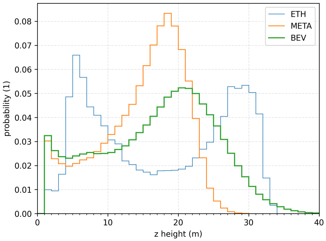
In parallel, the augmentation strategy was significantly expanded and fine-tuned to introduce greater diversity and variability during training. It was found early in this research that FABDEM did not fulfill the required quality criteria. ETH Zürich and META canopy model (see Figure 5 and Figure 6) were tested against Austrian ALS LiDAR data from the Austrian Federal Office of Metrology and Surveying [84]. META’s canopy models showed the most promising approximation of the globally available canopy datasets when compared to “ground truth” at the two Austrian validation sites. Both FABDEM and ETH Zürich’s Model (see Lang et al. [79]) produced unacceptably large artefacts in zones where apparently no trees were present.

FABDEM and ETH datasets were deemed to be unsuitable for micro scale wind modeling in light of the project’s accuracy requirements.

2.2.5. Wind Simulation

Using ECMWF ERA5 global circulation model (GCM) data series for accurate wind power predictions is an ongoing research topic with promising results (see Jourdier et al. [98], Gualtieri [99], Murcia et al. [100], Kuru [101], Schicker et al. [102], Gruber et al. [103], and Cheynet et al. [104]).

ERA5 grid point to point distance is approximately 30 km. Wind flow over unresolved orography is modeled by momentum sink (drag) terms (see ECMWF IFS documentation [105], p. 4 ff and Beljaars et al. [106]). In regions of high slopes and ruggedness, local wind speeds provided by global models can be corrected by forcing local high-resolution models with ERA5 grid scale variables as input (i.e., downscaling). There is extensive literature on downscaling methods and ERA5 bias corrections (see Wilczak et al. [107], Risser et al. [108], and Maciel-Tiburcio et al. [109]) but the field is lacking general consensus on an optimal simulation pathway. Dynamic downscaling is considered superior to statistical methods, albeit not extensively used due to higher computational costs compared to statistical methods. We use dynamic downscaling as best fitting approach to the established transient simulation runs in the sub-modules.

The validation was performed on the validation sites presented in Table 1. For some sites only single-sector simulations were run to use computational resources most effectively. The single sectors were chosen by the highest contribution to yearly wind energy production of all sectors. Experimental data at the single sector sites were filtered around the centered average simulated wind direction at the target with a sector angle of 22.5°. Single-sector simulations also enabled the research team to look at several diverse and complex sites and evaluate the model’s accuracy and run-time ahead of the two planned full simulation runs. The results of the single-sector runs are only representative of one incoming wind direction and cannot be generalized and used to evaluate the full wind potential of the validation site because contributions of all other sectors to the average power density are omitted. The results of the single sector runs are not fully comparable with 16 sector runs. This is reflected in the results statistics in in Section 4.1.

For two sites, all directions were simulated with an angular discretization of 22.5° (16 sectors). Additionally, two dynamic downscaling simulations for the fully simulated sites were run.

2.2.6. Validation of Isolated Model Hills

Relative isolation of the two model hills and upstream instrumentation allows precise definitions of inlet wind profiles and turbulence parameters. Comparing mean values and higher-order moments of downstream simulation results with measurements ensures model applicability according to similarity theory and for comparable terrain complexity. Results from the model hills are excluded from the six validation sites because of the a priori knowledge of upstream wind conditions.

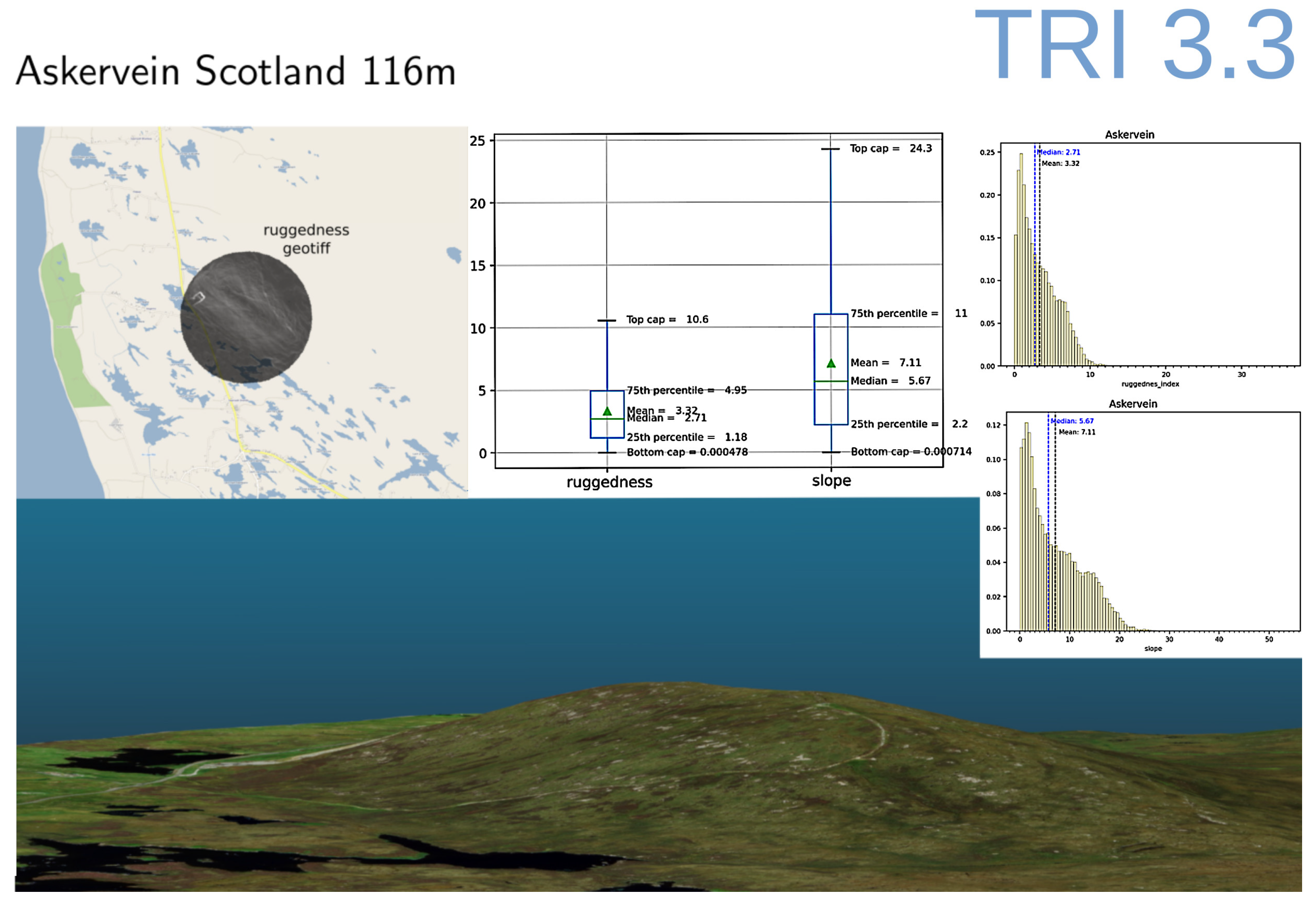
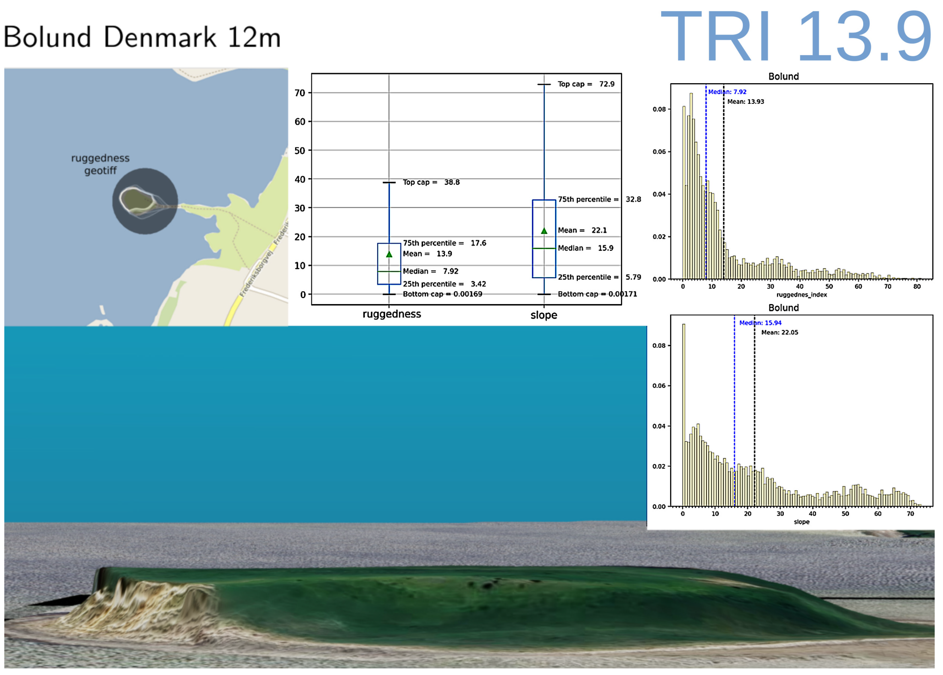
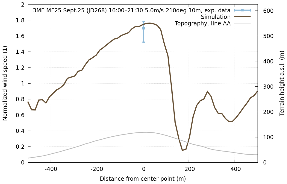
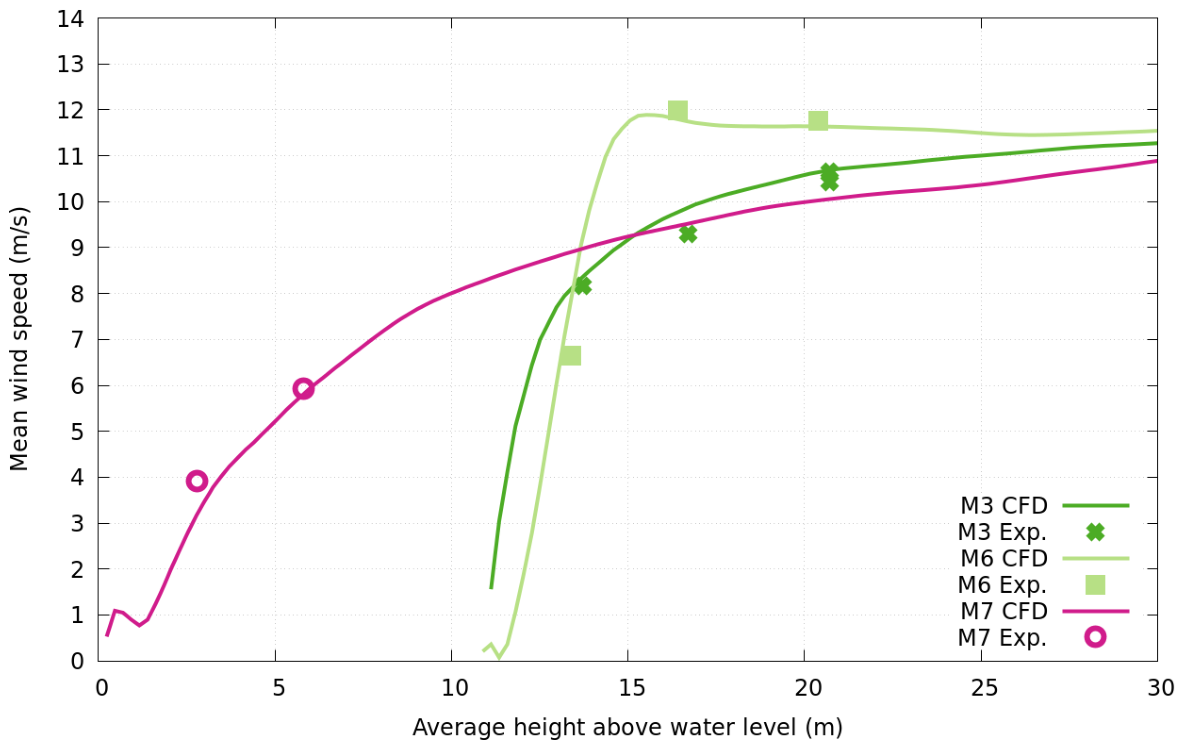
To demonstrate the suitability of the applied fluid dynamics models, we focused on two well-documented experiments. We used publicly available data from measurement campaigns at Askervein hill in Scotland (see Figure 7) and Bolund hill in Denmark (see Figure 8) to validate the turbulence model, solver, as well as geometry and meshing workflows for subsequent simulations.

As an indicator for orographic complexity, we used the terrain ruggedness index (TRI) as defined by Riley [110]. All calculations use 1 × 1 ${\mathrm{m}}^2$ pixels. Calculating area averaged TRI for both isolated model hills based on DTMs (see Ledoux et al. [78] for general topic overview) yields an average TRI = 13.9 for Bolund and average TRI = 3.3 for Askervein hill. The distinction between low-, medium-, and high-complexity terrain is not strictly defined in the known literature, but the present work focuses on terrain with higher TRI values. The average TRI for six validation sites (model hills Askervein and Bolund not included) is TRI = 7.3. To further characterize terrain ruggedness, histograms of TRI distribution are plotted for each site.

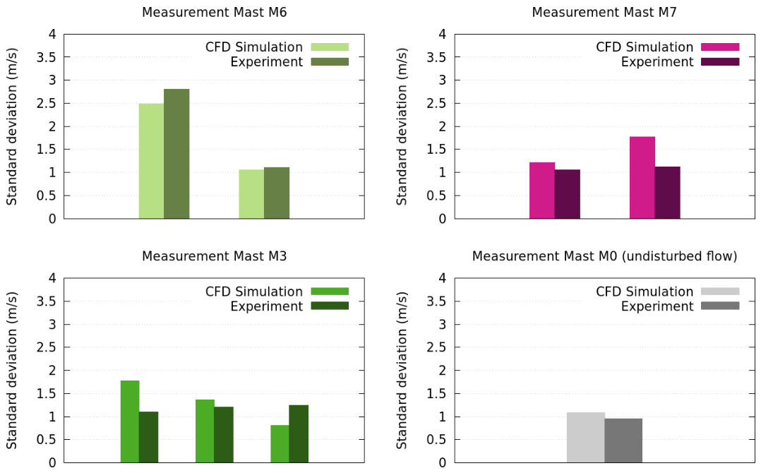
For both cases, the simulation results (see Figure 9 and Figure 10) from ensemble-averaged velocity magnitudes closely follow the measured average wind speed. At Bolund hill, the second-order moment (standard deviation of wind speed) follows measured quantities to a high degree (see Figure 11). It can be deduced from the validation of the model hills that from correct input data (wind speed and vertical profile) fairly accurate values for speed-up and turbulence intensity can be expected for similarly complex geometries. Askervein and Bolund are special cases nonetheless, because they have been carefully chosen for their relative isolation and meteorologically clearly defined in-flow conditions. For Bolund, the simulated 270° in-flow direction is over water and for Askervein, the simulated 210° catch is over flat and mostly featureless grassland.

The deeply analyzed model hills Askervein and Bolund are small in comparison to the other validated hills, but it is known from wind tunnel experiments that atmospheric-like flows have a large window of Reynolds number ($Re$) invariance.

$$Re={\displaystyle \frac{UL}{\nu }}$$

(2)

U is the velocity, L the typical length scale, and $\nu$ the kinematic viscosity of the fluid. Our model produces accurate results for the rather small model hills. Reynolds invariance allows for a 500× increase in Reynolds number while maintaining highly correlated velocities between rather small and realistically large geometries without breaking the model validity. The large window of Reynolds invariance of atmospheric flows enables transferability of modeling results from small to large hills. The same concept is applied in wind tunnel testing when downscaling real-world geometries (see Conan [111] for a practical wind tunnel example with Bolund hill and other complex terrain geometries).

2.2.7. Model Sensitivity Analysis for Different DEM and Canopy Data

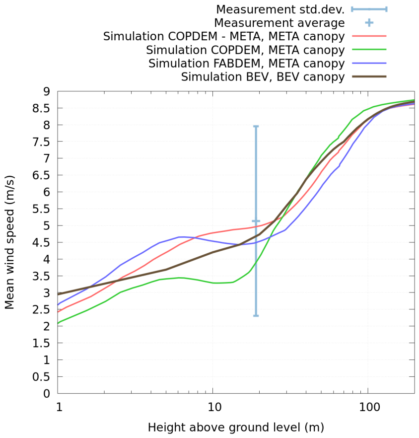
Sensitivity of simulated wind speed for different terrain and vegetation representations was tested for Lichtenegg site with NNW-sector. Following combinations of DEM, DTM and canopy models were simulated with identical CFD grid resolution, model settings, and boundary conditions:

• (COPDEM30 minus META canopy) with META CHM on top;
• COPDEM30 with META CHM canopy on top;
• FABDEM with META CHM canopy on top;
• BEV DTM with BEV nDSM canopy on top (considered as ground truth).

Figure 12 shows single-sector simulation results with those four different combinations of surface and canopy models. Note the logarithmic scale for height above ground level in the plot. For this sector and location, the simulation results for wind speed converge at 200 m above ground level. The highest model differences are found close to the ground where the vegetation cover and surface models show strong influence on wind speed. The closest trees (in case of the simulated NNW sector) are located 225 m up-stream from the measurement mast. If high-quality DTM and canopy data are not available for a specific site, the results indicate that (COMPDEM30 minus META) with META canopy on top is the next best choice to high-resolution laser scanning data regarding simulation accuracy. Putting vegetation on top of a DEM model, like COPDEM30, gives a strong negative bias close to the ground and potentially overestimates wind speeds at higher levels. FABDEM with META CHM on top and COPDEM30 with META on top both show unrealistic decrease in wind speed with height and should be avoided. Underestimation of wind speed in all four combinations is deemed due to the averaged and uncorrected ERA5 data at the inlet boundary.

Wind simulation is briefly described above and a graphical overview of the implemented modules and their connectivity is shown in Figure 1. The following sections describe setup, parameters, and model details used in our simulation workflow.

2.2.8. High-Resolution Sector-Wise Simulations

The four nearest grid points of ERA5 from the target are queried at ECMWF and a ten year interval of hourly (u,v) velocity data 100 m above ground level are downloaded, bilinear-interpolated, filtered by incoming wind sector, and averaged. The resulting 16 average velocities are used to generate vertical wind profiles that are surface normal to the inlet of each of the 16 sector-wise simulations with the average $\overline{(u,v)}$ given at 100 m above ground level at a roughness length value of $z_0$ = 0.03 [m] (inlet profile is identical to description in Section 2.2.9). A surface-fitted, hex-dominant mesh with a boundary layer (typically 99.9% cover of ground patch) is created separately for each of the 16 simulation domains. All meshes are created with blockMesh and snappyHexMesh from OpenFOAM-v2212. The high-resolution meshes use 148 million finite volume cells for Handalm and 68 million cells for Lichtenegg site. Mesh extents are 12 × 12 km² with a total domain height of 4 times the peak height difference of the generated 3D geometry. The background mesh size is 16 m and refinement zone at Level 3 with 6 cells between levels is applied to all cells below 20 m above ground (cut cells included) in the central high-resolution region of a 2 km diameter. The central region holds cells with porous media model enabled, which are created from canopy data described above. Leaf area density (LAD) $\lambda$ is simplified by a vertical step function $\lambda =(0{|}_{0<z\le 4\mathrm{m}},\lambda {|}_{z>4\mathrm{m}})$ assuming zero LAD from 0 to 4 m above ground level (z). Cells in the porous zone cell set have a Darcy–Forchheimer porosity model enabled where the momentum sink term S in OpenFOAM-v2212 is calculated by

$$S=-\left(\mu d+{\displaystyle \frac{\varrho }{2}}Uf\right)U$$

(3)

$\mu$ is the dynamic viscosity, $\varrho$ the fluid density, and U the velocity magnitude. In our model, the parameters are isotropic with Darcy parameter d = 0 and Forchheimer parameter f = 0.021. Outside the central region, only surface roughness lengths are mapped to the ground faces and no 3D porous zones are used. Initial time step size is calculated according to the CFL-criterion from inlet profile wind speed and minimum mesh sizes. Maximum Courant number in the domain is dynamically limited to 0.95 at run-time. Total simulation time for each sector depends on wind speed and streamwise domain length. First the theoretical, undisturbed stream-wise residence time based on the wind speed at 100 m above ground is calculated and 600 s are added for ensemble averaging. Ensemble averaging time resolution is not fixed and depends on the adaptive time step size. Typical time step size (and temporal ensemble averaging resolution) for Handalm North-sector was 0.197 s. LES turbulence model settings in OpenFOAM-v2212 are:

LESModel	SpalartAllmarasIDDES;
delta	IDDESDelta;
printCoeffs	on;
turbulence	on;
cubeRootVolCoeffs	deltaCoeff 1;
IDDESDeltaCoeffs	{hmax maxDeltaxyzCubeRoot; maxDeltaxyzCubeRootCoeffs {}}

The simulation result is the speed-up ratio of inlet wind speed to target wind speed. The inlet wind speed profile from averaged ERA5 (u,v) values often is not sufficiently accurate in rugged and mountainous terrain due to lack of spatial resolution in the ERA5 model. In case of high terrain ruggedness, the ensemble-averaged values of simulated wind speed at the target can not be used directly and need prior correction. We employ a two-step dynamic downscaling approach for wind speed correction that is explained below.

2.2.9. Lower-Resolution Dynamic Downscaling

Dynamic downscaling from bilinear interpolated ERA5 hourly data is performed on a lower-resolution mesh: Lateral resolution: 100 m, boundary layer mesh height: approx. 60 m, mesh extents: 22.3 × 22.1 km² at 4 times peak height of ground surface, total number of cells: 1.04 million. The same 3D input geometry as in the sector-wise high-resolution simulations is used for dynamic downscaling albeit with a much lower mesh resolution. Steady state boundary conditions from sector-wise runs are substituted for transient boundary conditions to enable direct input of linearly interpolated hourly ERA5 (u,v) vectors. The velocity boundary conditions as defined in OpenFOAM-v2212 for all vertical side patches of the simulation domain in the transient downscaling simulation are:

type	atmBoundaryLayerInletVelocity;
zDir	(0 0 1);
flowDir	table ((…));
Uref	table ((…));
Zref	100;
z0	uniform 0.03;
d	uniform 0;

zDir is the vector pointing in the “up” direction. flowDir and Uref are transient, tabulated and linear in time interpolated vectors from ERA5 $(u,v)$ data at 100 m above ground level. Zref is the reference height of wind speed (constant at 100 m). z0 is the surface roughness length and d the displacement height (see below in Equation (4)). flowDir is the normalised, transient $(u,v)$ vector from ERA5 and Uref the transient velocity magnitude (both at 100 m above ground level). The inlet height profile as implemented in OpenFOAM-v2212 is:

$$u={\displaystyle \frac{u^{*}}{\kappa }}ln\left({\displaystyle \frac{z-d+z_0}{z_0}}\right)$$

(4)

u is the wind speed at height z above ground level, $u^{*}$ is the friction velocity, $\kappa =0.41$ the Von Kármán constant and $z_0$ the surface roughness length. d is the zero plane displacement used for modeling upstream obstacles, and $d=0$ for all simulations.

One representative year is simulated with this setup and ensemble averaged at the target location with 100% time step coverage from 36,000 s (spin up time) until the end of the simulated year. The maximum Courant number is limited to 0.95 in the transient downsampling run. The results of the dynamic downscaling simulation is a coarse resolution, fully time resolved (with dynamic Co-Number limit of 0.95) wind speed at the target. Running a year-long transient simulation with fine mesh resolution is prohibitively expensive. The coarser mesh of the dynamic downscaling simulation is not suitable for direct wind speed prediction close to the ground level due to the lack of vertical resolution and thus underpredicts average wind speed at the target.

2.2.10. Numerical Schemes and Solution Strategy

Time is discretized by the backward scheme which is used in all simulations:

$${\displaystyle \frac{\mathsf{\partial }}{\mathsf{\partial }t}}\left(\varphi \right)={\displaystyle \frac{1}{\Delta t}}\left({\displaystyle \frac{3}{2}}\varphi -2{\varphi }^0+{\displaystyle \frac{1}{2}}{\varphi }^{00}\right)$$

(5)

t is simulation time, $\Delta t$ the time step size, and $\varphi$, ${\varphi }^0$, ${\varphi }^{00}$ denote current, last, and one before last field values. Backward scheme is implicit, second-order accurate, and transient. div($\varphi$, U) is discretized via Gauss LUST, Linear-Upwind Stabilized Transport, a blended scheme with following weights: 0.25 linear upwind, 0.75 linear. All other divergence discretizations are Gauss linear. Interpolation is linear and gradients are discretized by Gauss linear scheme. Solver tolerances are ${10}^{-7}$ for pressure p and ${10}^{-6}$ for both velocity U and $\tilde{\nu }$. Pressure field is solved by a GAMG (Generalized Geometric-Algebraic MultiGrid) solver with Gauss Seidel smoother and all other variables are solved with a smooth solvers and a symmetric Gauss Seidel smoother.

2.2.11. Lower-Resolution Sector-Wise Simulations

A total of 16 sector-wise simulations with coarser mesh resolution are run with the same model settings and parameters as the high-resolution runs described above. The frequency-weighted ensemble average velocity of the sector-wise simulations is compared to the ensemble-averaged velocity of the dynamic downscaling run to derive a correction factor.

2.2.12. Corrector Step

The local correction factor is defined as the ratio of average wind speed obtained by dynamic downscaling to the average wind speed obtained by frequency weighted, sector-wise, transient simulations with constant inlet profiles.

$$f_{corr}={\displaystyle \frac{{\overline{U}}_{dds,coarse}}{{\overline{U}}_{sec,coarse}}}$$

(6)

${\overline{U}}_{dds}$ is the ensemble averaged local velocity of the coarse downscaling simulation, ${\overline{U}}_{sec}$ is the ensemble averaged local velocity of the coarse resolution sector-wise simulation. $f_{corr}$ is calculated on the coarse meshes and can be applied to every point of interest in the simulation domain to correct the local high-resolution simulation velocity:

$${\overline{U}}_{corr,fine}=f_{corr}·{\overline{U}}_{fine}$$

(7)

${\overline{U}}_{corr,fine}$ is the corrected wind speed on the high resolution mesh, ${\overline{U}}_{fine}$ is the uncorrected ensemble averaged wind speed on the high resolution mesh. We apply $f_{corr}$ at the target location(s) to generate the corrected height profile of wind speed (as shown for Handalm and Lichtenegg validation sites).

2.2.13. Batch Processing and Data Analysis

Data retreival from ERA5, retreival and transformation of raster data for surface- and vegetation representation, parametric surface and vegetation geometry generation, 3D meshing of the finite volume mesh, roughness mapping, transient CFD simulation, ensemble averaging and wind speed correction are all achieved by a single-shot scripting system running on an Linux HPC cluster with SLURM workload manager as the underlying batch system to optimally distribute job execution and manage job dependencies. The driving logic and scripting is HPC-provider agnostic, and it was successfully run at different HPC providers on both ×86_64 and ARM processor architectures. Full simulation runs with 360/16° angle resolution were calculated on the Vienna Scientifc Cluster (VSC5) between 2 November 2023 and 30 September 2025. (https://asc.ac.at/systems/vsc-5/). For details of simulation set-up, see Section 2.2.8.

Post-processing of simulation data is automated and runs on the HPC system described above. Yearly average wind speeds are calculated by weighting sector-wise results on the high-resolution mesh by incoming wind frequency and multiplying by the correction factor $f_{corr}$. Weibull fitted wind speed distributions from ERA5 are scaled linearly by the corrected speed-up factor and used for calculating yearly average power densities in the simulation domain.

$$p\left(u\right)={\displaystyle \frac{k}{l}}·{\left({\displaystyle \frac{u}{l·f_{corr}}}\right)}^{(k-1)}·e^{-{\left({\displaystyle \frac{u}{l·f_{corr}}}\right)}^k}$$

(8)

$p\left(u\right)$ is the probability of wind speed u at the target. k and l are frequency-weighted Weibull parameters fitted to ERA5 data series of incoming wind.

3. Results

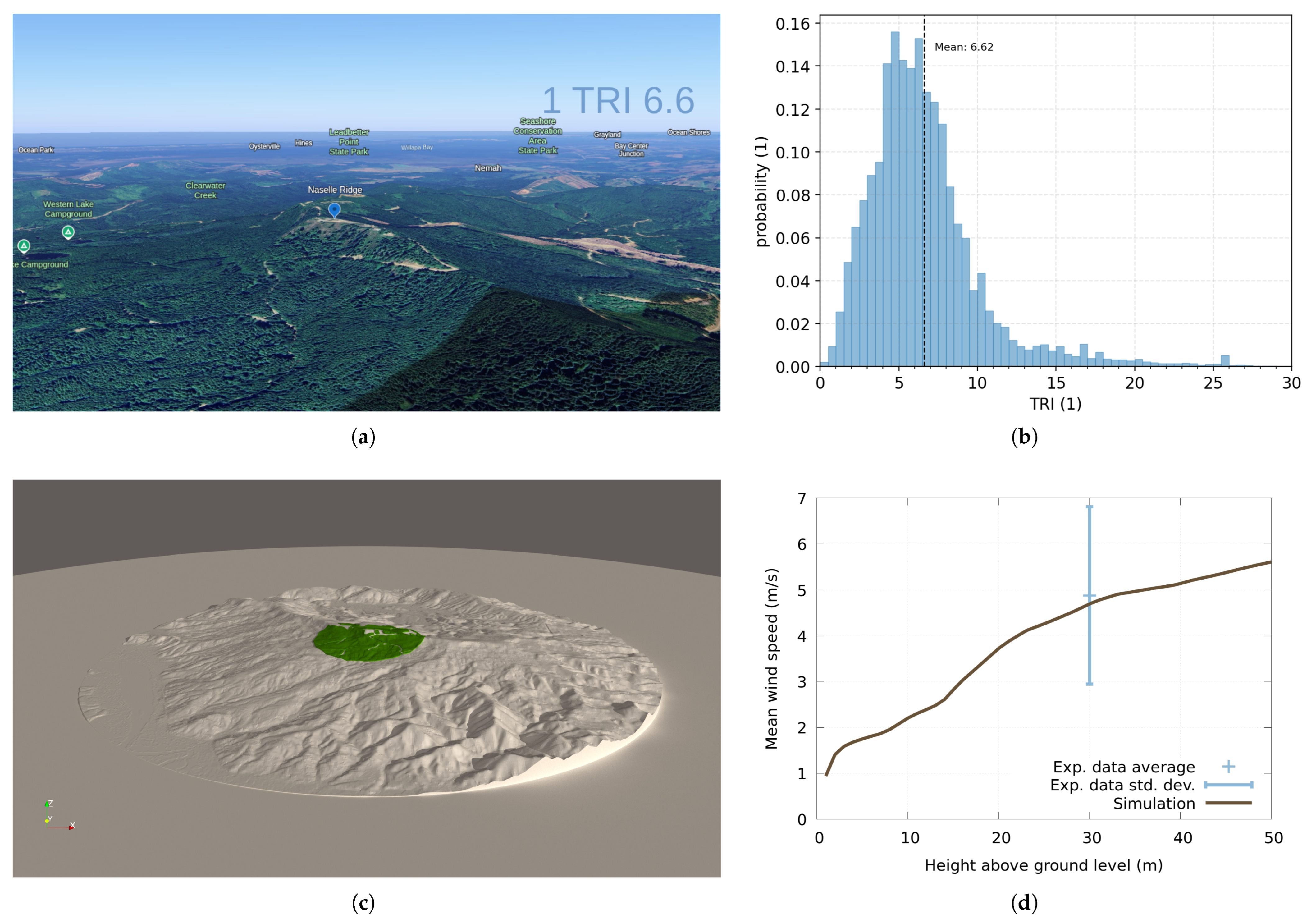
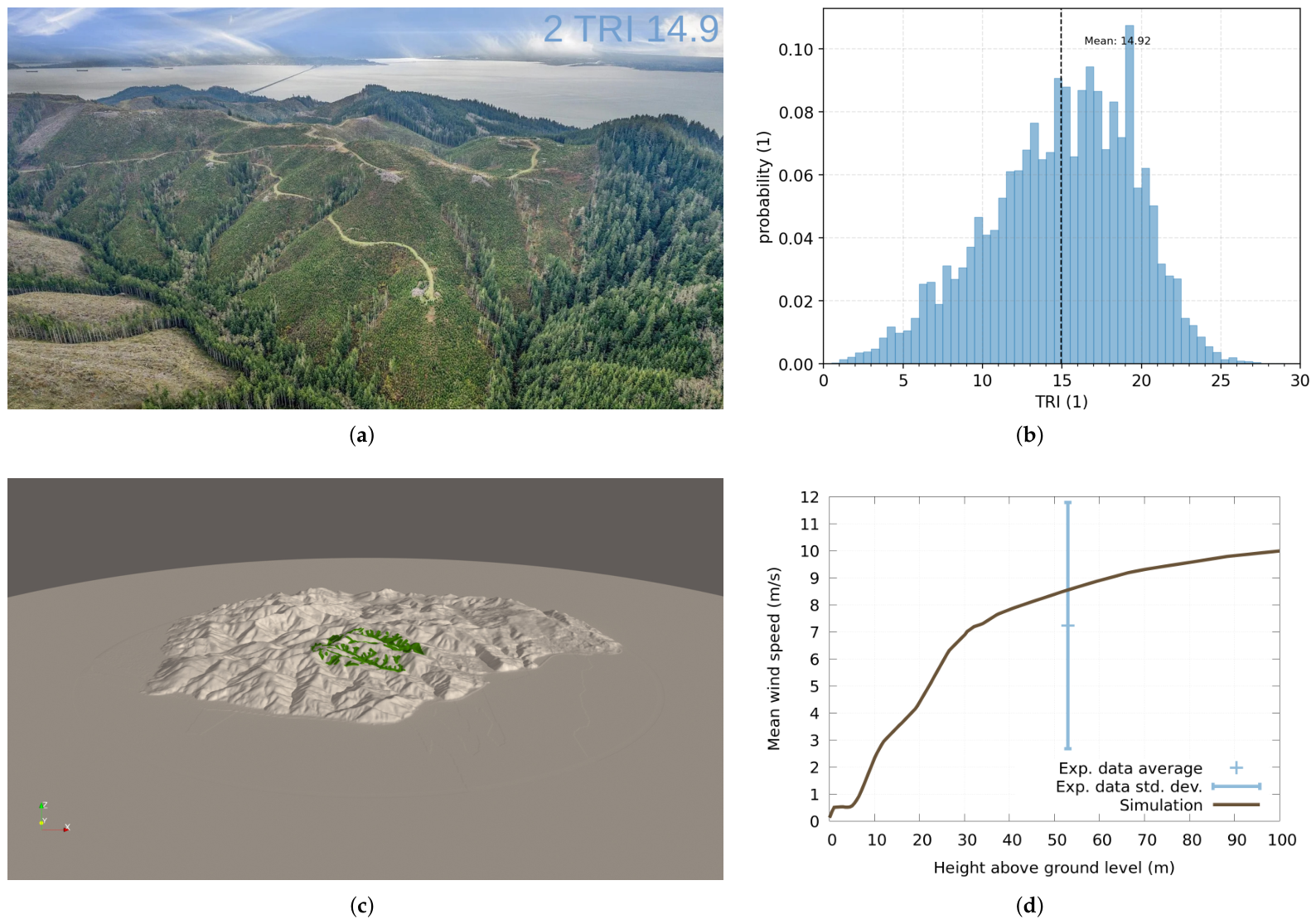
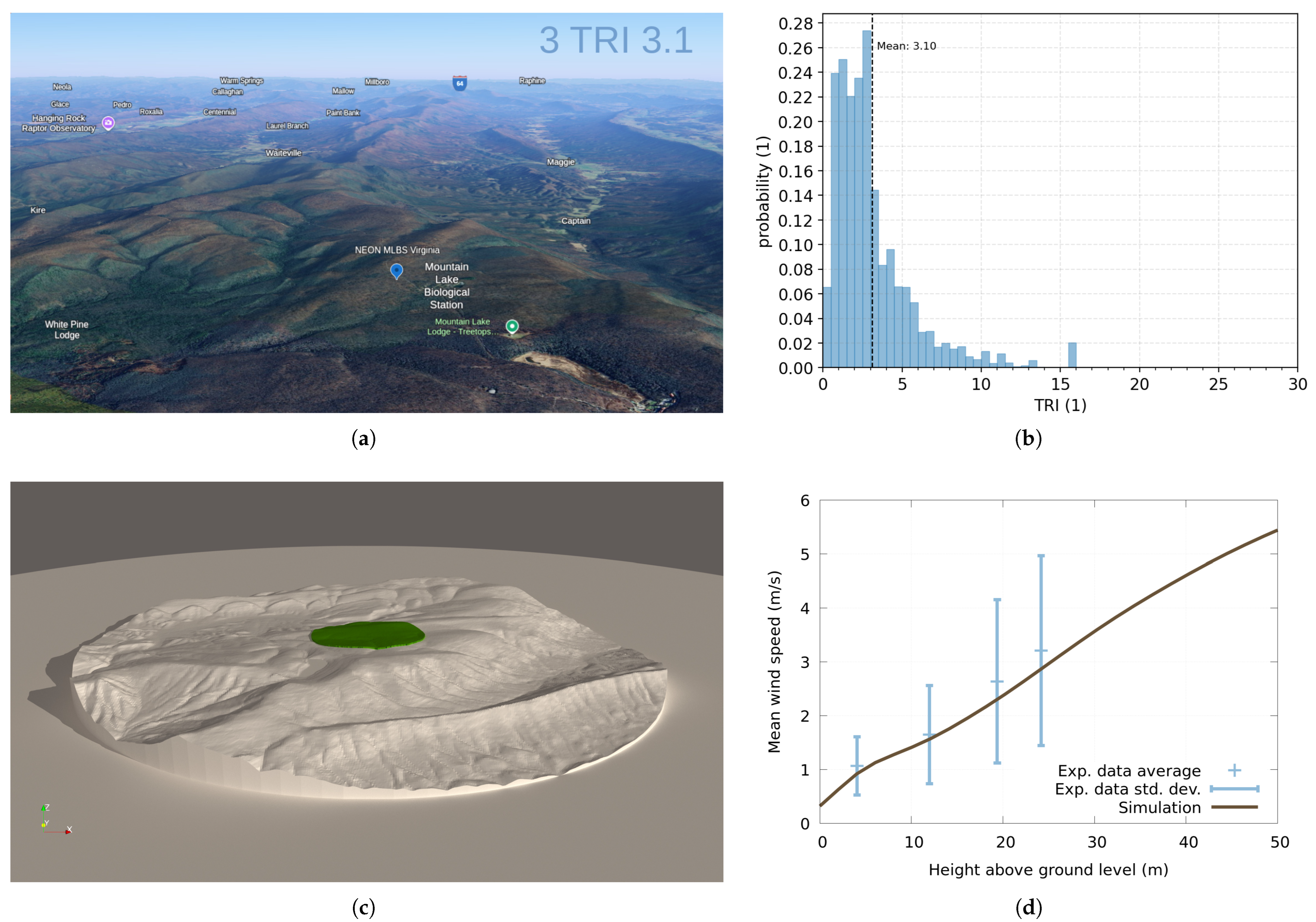
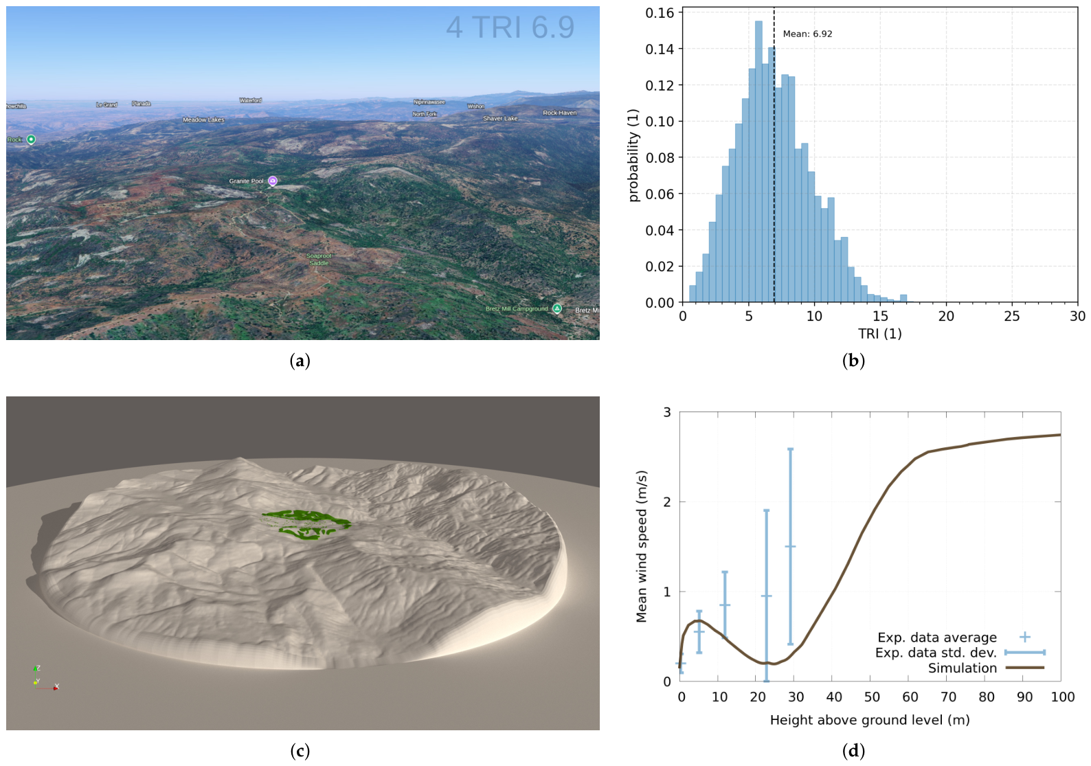
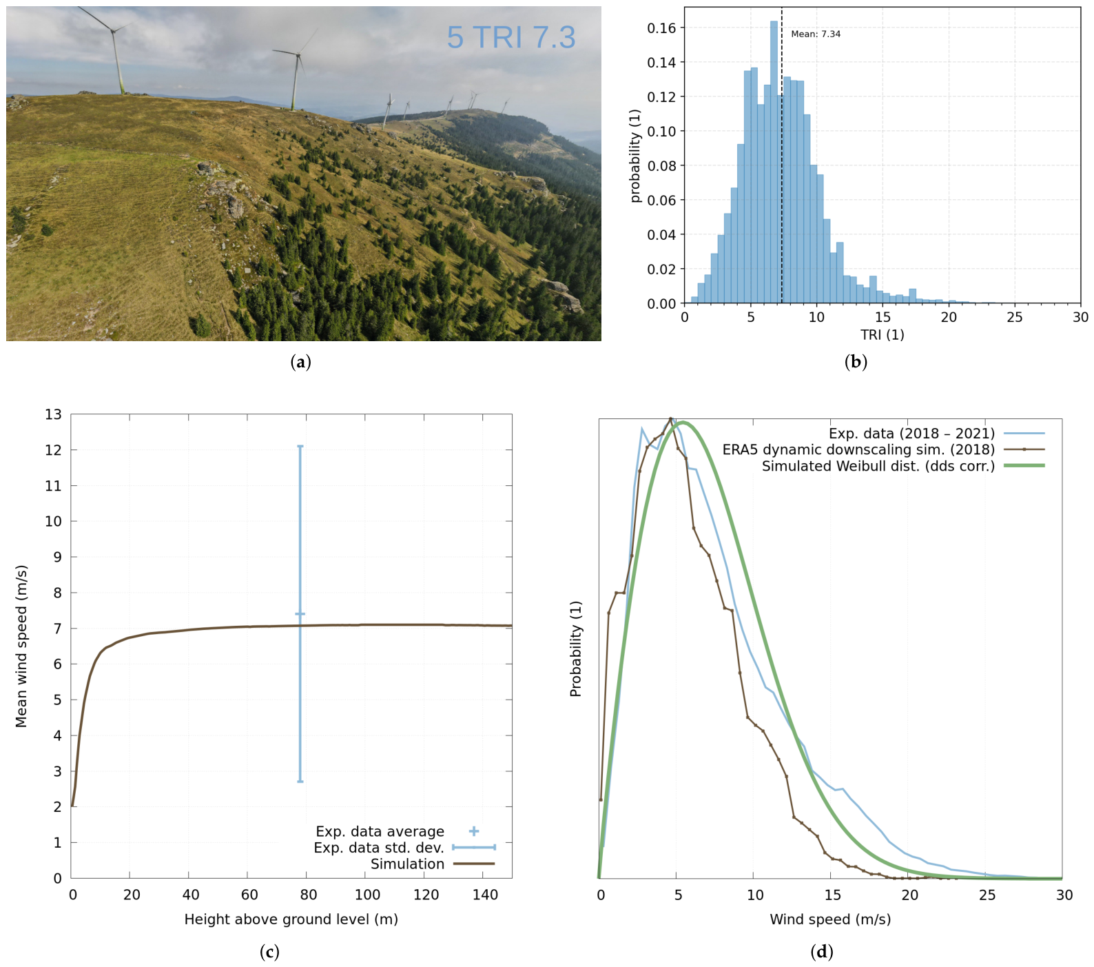
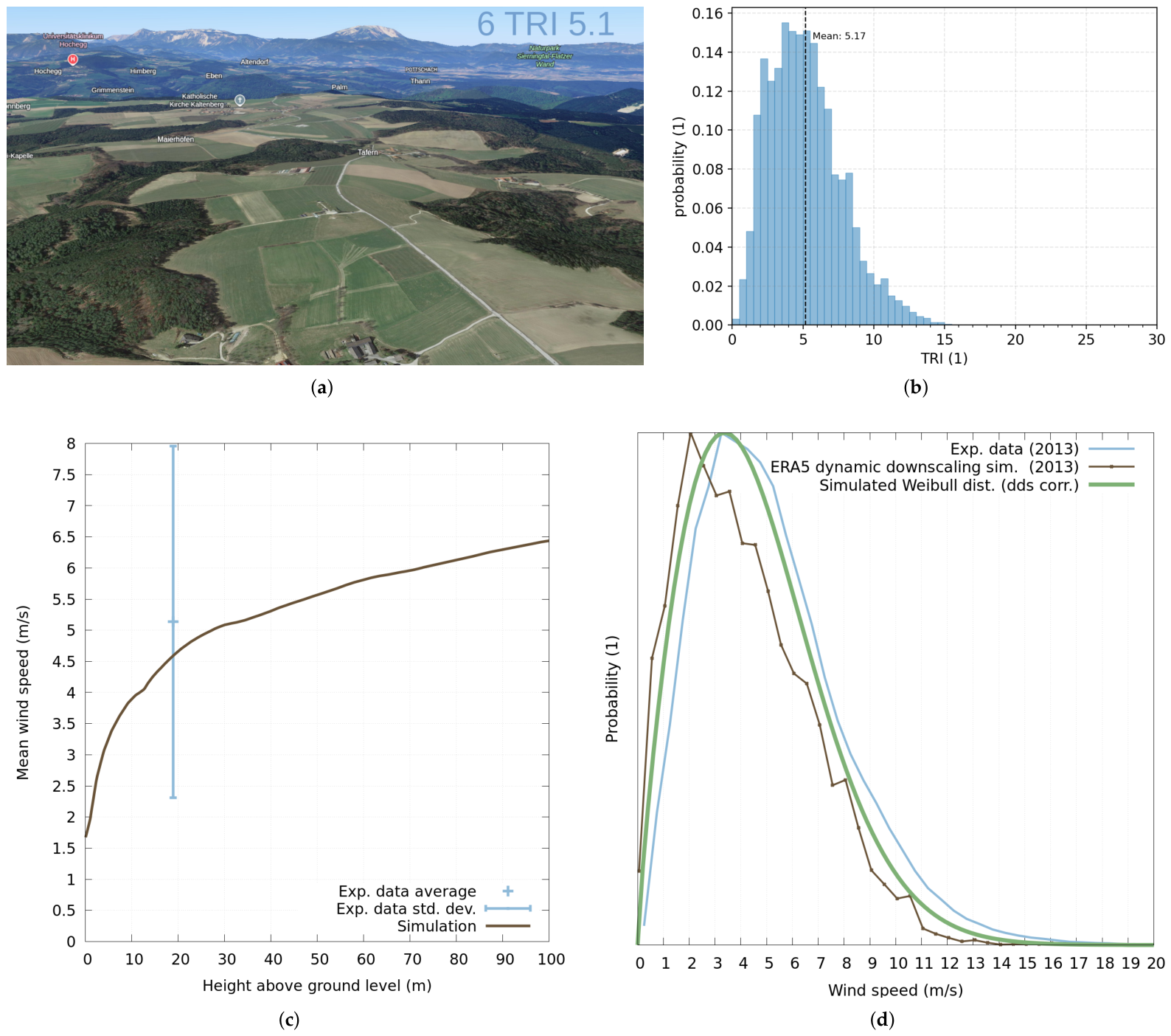
In this section, we describe simulation results for the validation sites in medium- to high-complexity terrain where long-term, high-quality, and well-documented experimental data were available. Results include a site description with overview photographs or images from Google Earth, a histogram of the Terrain Ruggedness Index (TRI), and a comparison of experimental and simulated wind speeds. See results figure index in

Table 2. Summary of validation site locations and associated figures.

Ref	Site Name (Exp. Data Provider), State	Figure
1	Naselle Ridge (tall tower dataset), USA	Figure 13
2	Megler (tall tower dataset), USA	Figure 14
3	Mtn. Lake Biological Station (NEON), USA	Figure 15
4	Soaproot Saddle (NEON), USA	Figure 16
5	Handalm wind park (E-Stmk), AT	Figure 17, Figure 18 and Figure 19
6	Lichtenegg research wind park (FHTW), AT	Figure 20, Figure 21 and Figure 22

.

Below, each validation site is characterized by a topology overview and a TRI histogram. The simulation result is given as a height profile of average wind speed at the target compared to the experimental average and standard deviation of measurement data for the simulated sector(s).

3.1. Overview and Results of Site 1—Naselle Ridge

We characterize Naselle Ridge as a moderately complex site (see Figure 13). The simulated height profile of the NW sector matches the experimental data at the target with excellent accuracy.

3.2. Overview and Results of Site 2—Megler

Megler (see Figure 14) is an outlier in many respects compared to the other validation sites. It features the highest average TRI of all examined sites with a broader TRI distribution than all other simulated sites. The forested areas are very patchy with forest clearings close to the measurement tower that changed in size during the measurement campaign (according to historical satellite images). Megler is located near the sea/land transition zone, where ERA5 often does not yield reliable results (also see Alkhalidi et al. [113]). All those factors together lead to a significant over-estimation of wind speed for the southern sector. Furthermore, sector-wise analysis at Megler reveals a damped response in the south-eastern sectors compared to the ERA5 wind rose, which might indicate some lee side effects of the measurement tower on the anemometer. Megler is a site that exposes the limits of the presented method and leaves some questions open that can not be fully answered by the available data.

3.3. Overview and Results of Site 3—Mountain Lake Biological Station

The measurement mast at Mountain Lake Biological Station (MLBS) is located in a large forest (see Figure 15) and was chosen to verify momentum sink model parameters for different heights directly within the vegetation zone. The simulation results of wind velocities from WNW sector closely follow experimental data. Wind conditions at MLBS target height are unsuitable for wind power applications. Power density calculation, based on the linear scaling of Weibull parameters within the forest zone, does not yield results with an acceptable error range. It is assumed that the resistance parameter of the forest canopy might be lower in the z-direction compared to the lateral resistances due to the swaying motion of the tree tops.

3.4. Overview and Results of Site 4—Soaproot Saddle

Soaproot Saddle site measurement mast is located in (moderately) complex terrain (see Figure 16). Intermittent flow separation at the target is simulated for the S sector. Average wind speeds are generally too low for wind power applications. The vegetation layer close to the met-mast recently changed strongly due to forest fires. Considering all the complications above, the errors of the presented method are interpreted as acceptable for the intended cause. Site suitability for wind power applications can be ruled out with high confidence at Soaproot Saddle.

3.5. Overview and Results of Site 5—Handalm

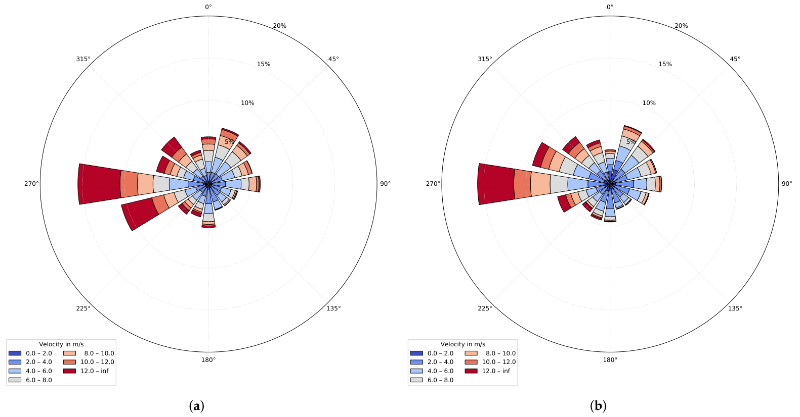
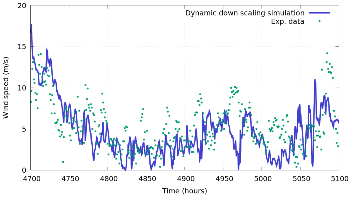
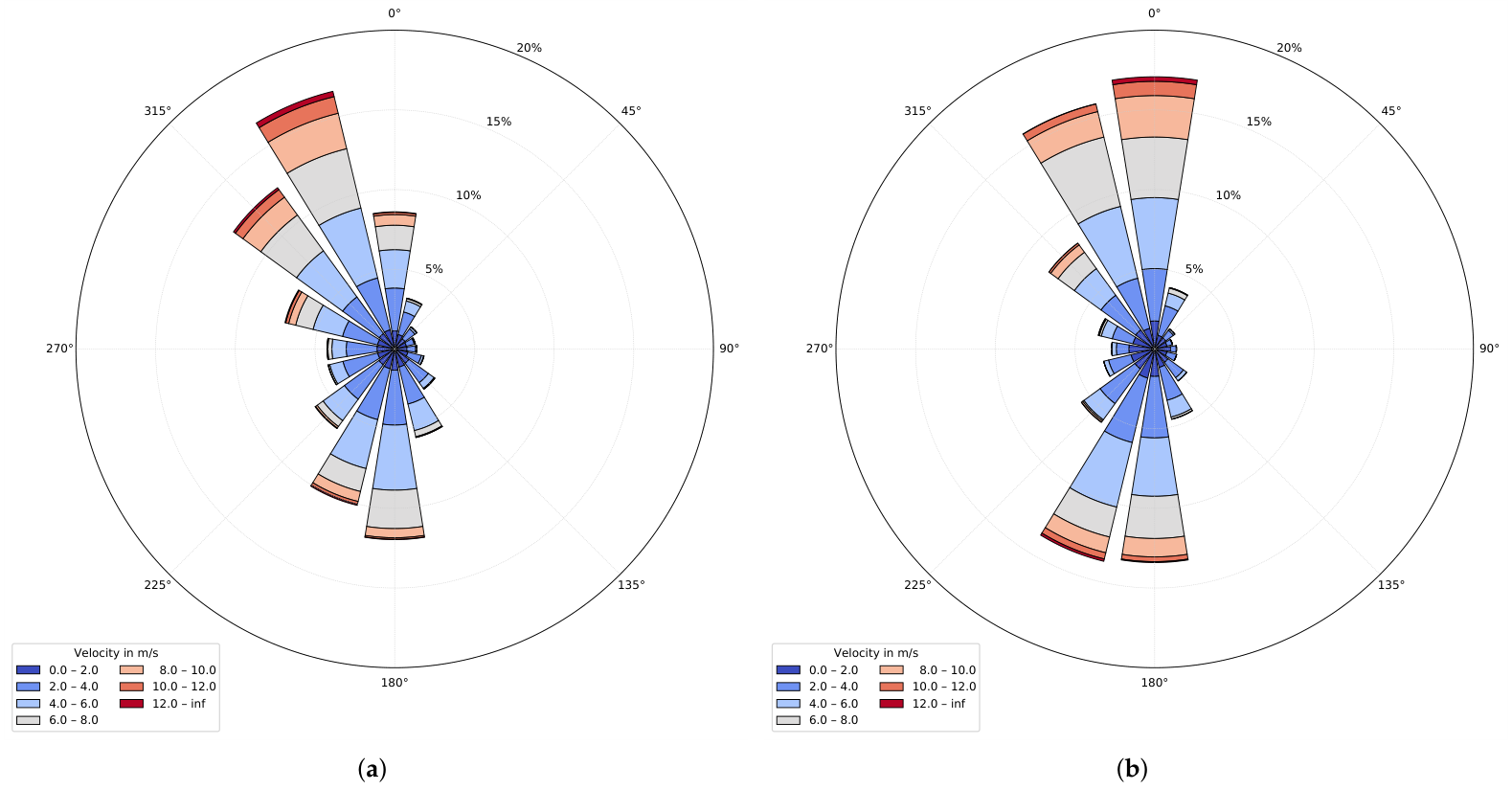
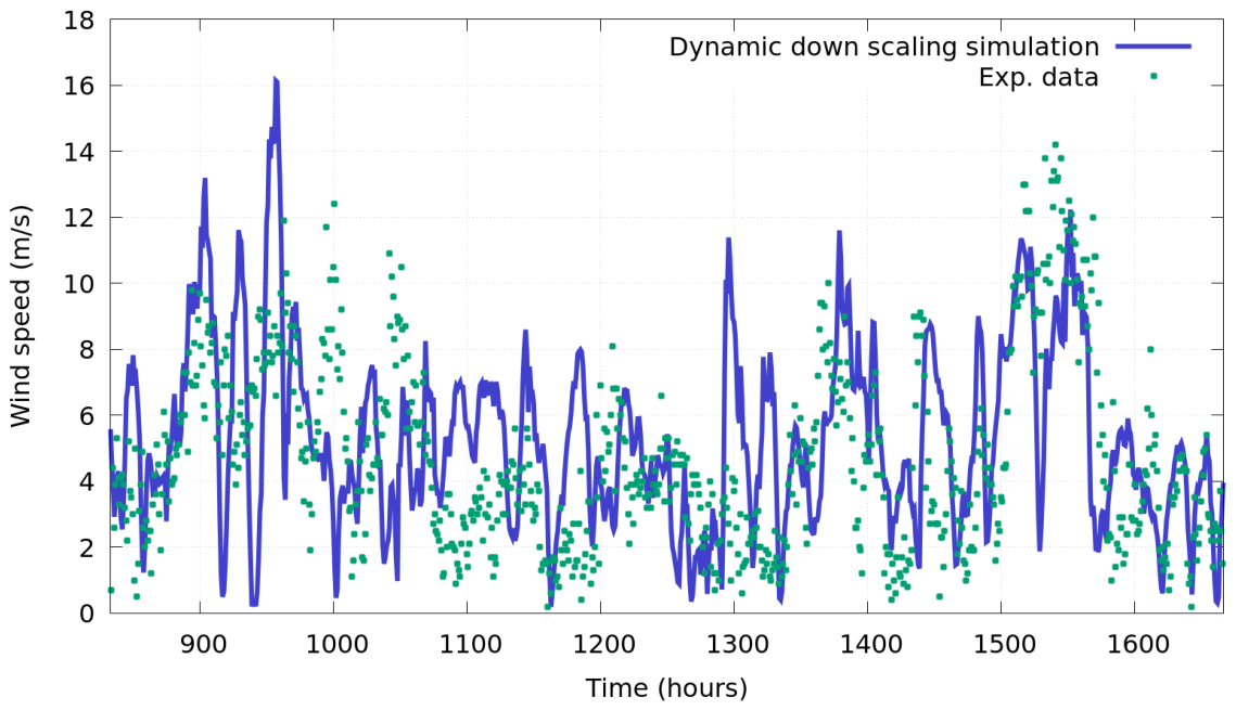
For the Handalm site (see Figure 17), actual production data were available. This was provided by local Austrian Energy company Energie Steiermark AG, Graz, Austria. A total of 16 sectors were simulated and dynamic downscaling of ERA5 data was performed. The result of the average wind speed closely matches experimental data. The wind rose analysis of dynamic downscaling results shows very good agreement with measured values. The higher-up measurement position of 78 m above ground, distance to ground level vegetation, and a fairly flat wind profile on the mountain top are favorable to the coarse downscaling simulation. Apart from smaller shifts in frequency distribution, the correlation of downscaling simulation results with experimental data is high (see Figure 18). Sub-daily variations of experimental data and dynamic down scaling simulation are shown in Figure 19.

3.6. Overview and Results of Site 6—Lichtenegg

Lichtenegg site (see Figure 20) is unique due to low anemometer fixing heights and (moderately) complex terrain as well as strongly varying vegetation patterns all around the location. 16 sectors were simulated and dynamic downscaling of ERA5 data was performed. There is still some significant offset of the simulated profile compared to the experimental data. A site visit revealed large, seasonally changing fields with crops and intermittently high grassland directly around the measurement mast. The periodically changing roughness length due to agricultural activities and the relatively low fixing position of the anemometer might be significant factors for explaining the differences to the simulated values. The wind rose analysis of dynamic downscaling results shows quite good agreement with measured values. The frequency of North-, South-south-west and South-west sectors are over estimated by the downscaling simulation but the general shape, dominant wind directions and velocity distributions match reasonably well with experimental data (see Figure 21). Sub-daily variations of experimental data and dynamic down scaling simulation are shown in Figure 22.

4. Discussion

4.1. Findings

A fully automated wind simulation workflow was validated on a selected set of measurement sites in complex terrain with high ruggedness index and diverse vegetation cover. Validation results for predicted average wind speed and average power density for the given period are shown in

Table 3. Summary of validation site locations ¹ and number of simulated wind directions.

Ref	Site Name	Year(s)	z	${\mathbf{U}}_{\mathbf{sim}}$	${\mathbf{U}}_{\mathbf{exp}}$	${\mathbf{pd}}_{\mathbf{sim}}$	${\mathbf{pd}}_{\mathbf{exp}}$	${\mathit{ϵ}}_{\mathbf{U}}$	${\mathit{ϵ}}_{\mathbf{pd}}$
			$\left[\mathbf{m}\right]$	$[\mathbf{m}/\mathbf{s}]$	$[\mathbf{m}/\mathbf{s}]$	$[\mathbf{W}/{\mathbf{m}}^{\mathbf{2}}]$	$[\mathbf{W}/{\mathbf{m}}^{\mathbf{2}}]$	$[\%]$	$[\%]$
1	Naselle Ridge	2011–2017	30	4.71	4.88	91	109	−3.5	−16.5
2	Megler	2011–2017	53	8.53	7.23	685	569	+18.0	+20.4
3	MLBS	2016–2022	24	3.07	3.21	15	72	−4.4	−79.2
4	Soaproot S.	2017–2023	12	0.48	0.88	0.23	8.57	−45.5	−97.4
5	Handalm	2018	78	7.13	7.41	446	541	−3.8	−17.6
6	Lichtenegg	2013	19	4.61	5.04	126	171	−8.5	−26.3

¹ Site 4, Soaproot Saddle, is not included in the statistics below due to simulated intermittent recirculation at the measurement site and yet unsolved analysis problems in experimental data to filter for and determine the corresponding wind direction.

. An overview of method accuracy based on tested sites is given in

Table 4. Summary of simulation method accuracy based on simulated sites included in the statistics.

Ref.	Simulated Sectors	MAE	RMSE	Wind Speed Error	Power Density Error
		$[\mathbf{m}/\mathbf{s}]$	$[\mathbf{m}/\mathbf{s}]$	Average $[\%]$	Average $[\%]$
1, 2, 3	1	0.54	0.76	3.4	−25.1
5, 6	16	0.36	0.36	−6.2	−22.0

.

z denotes the height of the wind measurement instrument above (local) ground level. $U_{sim}$ is the simulated average wind speed at height z. $U_{exp}$ is the experimental average value at height z. $p{d}_{sim}$ is the simulated average wind power density at height z. $p{d}_{exp}$ is the experimental average power density at height z. ${ϵ}_U$ is the error (in percent) between simulated and experimental average wind speeds. ${ϵ}_{pd}$ is the error (in percent) between simulated and experimental wind power density.

Mean absolute error (MAE) and root mean square error (RMSE), percentage error of wind speed, and power density prediction are shown below in Table 4.

$$MAE={\displaystyle \frac{1}{n}}{\displaystyle \sum _1^n}\left|U_{sim}-U_{exp}\right|$$

(9)

$$RMSE=\sqrt{{\displaystyle \frac{1}{n}}\sum _1^n{\left(U_{sim}-U_{exp}\right)}^2}$$

(10)

n is the number of samples, $U_{sim}$ is the simulated velocity, $U_{exp}$ is the experimental velocity.

Results for Sites 1, 2 and 3 are validation results for a single sector with the highest power density (based on ECMWF ERA5 statistics). For Sites 5 and 6, all 16 sectors with 360° coverage were simulated and frequency-weighted.

Site 3 is a special case and should be evaluated as such. This site is unsuitable for wind power applications due to low wind speeds at the investigated hub heights. Simulation results show that the applied models perform well (considering wind speed deviations) within dense vegetation zones below the forest canopy height.

Simulation results at Site 2 (Megler) have quite a high deviation of measured wind speed. It must be underlined that Megler has exceptionally high terrain complexity (TRI), high uncertainty regarding vegetation cover and canopy heights as well as high input data uncertainty of ERA5 data. ERA5 produces lower accuracy data close to coastal areas. A detailed analysis of reduced ERA5 accuracy at sea/land transitions is found in Alkhalidi et al. [113]. At the current development state of our model and data pipeline, the use of ERA5 as input data in regions close to coasts will introduce significant errors in wind speed and subsequently reduce simulation accuracy. In coastal regions, the model can still be used to reliably find the locations with the highest relative wind speeds in complex terrain, but due to the nature of ERA5 input data the absolute results (e.g., power density) close to coasts should not be used directly for de-risking long-term investments without further data input like close by wind measurement masts or on-site LiDAR. As a general guideline, at least a distance of one ERA5 cell (approximately 30 km) should be kept to coastal regions for sufficiently accurate results.

Sites 5 and 6 were simulated using the full workflow described in Section 2.2.1. For applicability in wind engineering applications, those two cases should be considered typical as they cover all wind directions (16 sectors, 360°) and dynamic downscaling of weather data.

4.2. Accuracy Comparison

To put the accuracy of our method into perspective, we compare our results to Global Wind Atlas (GWA at https://globalwindatlas.info/, accessed on 23 January 2026). At the Handalm site, GWA yields a power-density of 1169 W/m², an overprediction by 116% compared to experimental data. At the Lichtenegg site, GWA yields a wind power density of 209 W/m² already at 10 m above ground level, which is 22% higher than the experimental value at 19 m above ground level (19 m value is not available via GWA). For both fully validated cases, we see an extreme over-prediction of wind power densities by the GWA compared to measured data.

4.3. Current Shortcomings and Future Research Goals

Our method tends to underestimate wind power densities. The reasons for this bias to lower simulated power densities in our model, compared to experimental data, is not fully understood yet. One reason for systematic under-prediction could be negative ERA5 wind speed bias in the alpine region. Switching the input data generation from ERA5 to a higher-resolution model could improve inlet wind speed accuracy and reduce data bias in high-complexity terrain. A promising candidate of a local weather model in the wider alpine region is AROME (Application of Research to Operations at MEsoscale) by Geosphere Austria. AROME offers 2.5 km grid resolution and is available within the bounding box 42.98–51.82°N, 5.49–22.1°E. Data mapping and forcing of OpenFOAM by AROME data (to adhere to the established workflow with OpenFOAM as the main engine) might be a rewarding research endeavor. To tackle ERA5 uncertainties in coastal regions, nesting global models like ERA5 and higher resolution WRF models would correct errors introduced by ERA5, but at significant cost for downscaling global circulation data onto rugged terrain at high local resolution to capture sufficient terrain details influencing flow patterns.

Further research and additional validation runs with higher quality terrain and vegetation data as well as testing other downscaling approaches are needed to determine the root causes of inaccuracies and improve surface-, vegetation-, and wind-models without compromising on simulation result reliability.

5. Conclusions

An automated method without need for local calibration to accurately simulate wind speed in complex terrain was presented. Results for two validation runs with 16 sectors were shown. The sites are in complex, mountainous terrain with patchy and strongly varying vegetation layers. Simulation results of average wind speed and wind power density are suitable for site assessment of wind power applications at low and at high hub-heights.

The causes for a slightly negative bias should be further investigated. The method currently also shows reduced accuracy at locations with high wind speed variability between ERA5 grid points, like the on-shore/off-shore transition regions. Validating more sites in complex terrain using our model will bring deeper insights into this method’s application range.

Further open work is the consideration of other key parameter layers, like buildings. Forest and vegetation layers are included in the current version. New generations of global datasets generated by machine learning methods, like the Global Building Atlas by the Munich University of Technology (TUM), is planned for inclusion in future versions. This will enable covering both forest canopy and buildings, especially in remote areas where other building datasets like OSM are notoriously sparse. Better understanding of tree top dynamics in dense deciduous and coniferous forests will improve porous media modeling and wind speed accuracy in forested areas. Accuracy enhancements close to the ground level could be highly beneficial to small wind power applications at typically lower hub heights.

References

1. Lee, J.C.Y.; Fields, M.J. An overview of wind-energy-production prediction bias, losses, and uncertainties. Wind Energy Sci. 2021, 6, 311–365. [Google Scholar] [CrossRef]
2. Barber, S.; Schubiger, A.; Koller, S.; Eggli, D.; Radi, A.; Rumpf, A.; Knaus, H. The wide range of factors contributing to wind resource assessment accuracy in complex terrain. Wind Energy Sci. 2022, 7, 1503–1525. [Google Scholar] [CrossRef]
3. Barber, S.; Schubiger, A.; Koller, S.; Eggli, D.; Radi, A.; Rumpf, A.; Knaus, H. A New Decision Process for Choosing the Wind Resource Assessment Workflow with the Best Compromise between Accuracy and Costs for a Given Project in Complex Terrain. Energies 2022, 15, 1110. [Google Scholar] [CrossRef]
4. Badger, J.; Hahmann, A.; Larsén, X.G.; Badger, M.; Kelly, M.; Olsen, B.T.; Mortensen, N.G. The Global Wind Atlas: An EUDP Project Carried Out by DTU Wind Energy; Technical report; DTU: Copenhagen, Denmark, 2015. [Google Scholar]
5. Hahmann, A.N.; Sīle, T.; Witha, B.; Davis, N.N.; Dörenkämper, M.; Ezber, Y.; García-Bustamante, E.; González-Rouco, J.F.; Navarro, J.; Olsen, B.T.; et al. The making of the New European Wind Atlas—Part 1: Model sensitivity. Geosci. Model Dev. 2020, 13, 5053–5078. [Google Scholar] [CrossRef]
6. Dörenkämper, M.; Olsen, B.T.; Witha, B.; Hahmann, A.N.; Davis, N.N.; Barcons, J.; Ezber, Y.; García-Bustamante, E.; González-Rouco, J.F.; Navarro, J.; et al. The Making of the New European Wind Atlas—Part 2: Production and evaluation. Geosci. Model Dev. 2020, 13, 5079–5102. [Google Scholar] [CrossRef]
7. Mann, J.; Angelou, N.; Arnqvist, J.; Callies, D.; Cantero, E.; Arroyo, R.C.; Courtney, M.; Cuxart, J.; Dellwik, E.; Gottschall, J.; et al. Complex terrain experiments in the New European Wind Atlas. Philos. Trans. A 2016, 375, 20160101. [Google Scholar] [CrossRef]
8. Davis, N.N.; Badger, J.; Hahmann, A.N.; Hansen, B.O.; Mortensen, N.G.; Kelly, M.; Larsén, X.G.; Olsen, B.T.; Floors, R.; Lizcano, G.; et al. The Global Wind Atlas: A High-Resolution Dataset of Climatologies and Associated Web-Based Application. Bull. Am. Meteorol. Soc. 2023, 104, E1507–E1525. [Google Scholar] [CrossRef]
9. Blocken, B.; Stathopolous, T.; Carmeliet, J. CFD Simulation of the Atmospheric Boundary Layer: Wall Function Problems. Environment 2007, 41, 238–252. [Google Scholar] [CrossRef]
10. Adib, J.; Langner, J.; Alletto, M.; Akbarzadeh, S.; Kassem, H.; Steinfeld, G.; Stoevesandt, B.; Letzel, M. On the necessity of automatic calibration for CFD based wind resource assessment. Preprint 2021. [Google Scholar] [CrossRef]
11. Taylor, P.; Teunissen, H. Askervein ’82: Report on the September/October 1982 Experiment to Study Boundary Layer Flow over Askervein, South Uist; Technical report; Report: MSRB-83-8; Meteorological Services Rersearch Branch, Atmospheric Environment Service, Ontario, Environment Canada, Atmospheric Research: Ontario, Canada, 1983.
12. Taylor, P.A.; Teunissen, H. The Askervein Hill Project: Report on the Sept./Oct. 1983, Main Field Experiment; Technical report; Meteorological Services Research Branch, Atmospheric Environment Service, Ontario, Environment Canada, Atmospheric Research: Ontario, Canada, 1985.
13. Gravdahl, A.R. Wind Field Simulations at Askervein Hill; Technical report; Internal study; Vector AS: Tønsberg, Norway, 1999. [Google Scholar]
14. Spalart, P. The Uses of DES: Natural, extended and improper. In Proceedings of the DESider, Stockholm, Sweden, 14–15 July 2005. [Google Scholar]
15. Spalart, P.; Deck, S.; Shur, M.L.; Squires, K.D.; Strelets, M.K.; Travin, A. A new version of detached-eddy simulation, resistant to ambiguous grid densities. Theor. Comput. Fluid Dyn. 2006, 20, 181–195. [Google Scholar] [CrossRef]
16. Bechmann, A. Results of the Blind Comparison; Technical report; DTU: Riso, Denmark, 2009. [Google Scholar]
17. Bechmann, A.; Berg, J.; Courtney, M.S.; Jørgensen, H.E.; Mann, J.; Sørensen, N.N. The Bolund Experiment: Overview and Background; Technical report; DTU: Riso, Denmark, 2009. [Google Scholar]
18. Bechmann, A.; Sørensen, N.N.; Berg, J.; Mann, J.; Rethore, P. The Bolund Experiment, Part II: Blind Comparison of Microscale Flow Models. Bound.-Layer Meteorol. 2011, 141, 245–271. [Google Scholar] [CrossRef]
19. Berg, J.; Mann, J.; Bechmann, A.; Courtney, M.S.; Jørgensen, H.E. The Bolund Experiment, Part I: Flow over a Steep, Three-Dimensional Hill. Bound.-Layer Meteorol. 2011, 141, 219–243. [Google Scholar] [CrossRef]
20. Diebold, M.; Higgins, C.; Fang, J.; Bechmann, A.; Parlange, M.B. Flow over Hills: A Large-Eddy Simulation of the Bolund Case. Bound.-Layer Meteorol. 2013, 148, 177–194. [Google Scholar] [CrossRef]
21. Yeow, T.S.; Cuerva-Tejero, A.; Perez-Alvarez, J. Reproducing the Bolund Experiment in Wind Tunnel; Technical report; Universidad Politecnica de Madrid: Madrid, Spain, 2014. [Google Scholar]
22. Yeow, T.S.; Cuerva, A.; Conan, B.; Pérez-Álvarez, J. Wind Tunnel Analysis of the Detachment Bubble on Bolund Island. J. Phys. Conf. Ser. 2014, 555, 012021. [Google Scholar] [CrossRef]
23. Lange, J.; Mann, J.; Angelou, N.; Berg, J.; Sjöholm, M.; Mikkelsen, T. Variations of the Wake Height over the Bolund Escarpment Measured by a Scanning Lidar. Bound.-Layer Meteorol. 2015, 159, 147–159. [Google Scholar] [CrossRef]
24. Cuerva-Tejero, A.; Gallego-Castillo, C.; Lopez-Garcia, O.; Perez-Alvarez, J.; Yeow, T. Comparison of Full Scale and Wind Tunnel Measurements of the Spatial Distribution of Turbulence Components over the Bolund Island; Technical report; Universidad Politénica de Madrid: Madrid, Spain, 2015. [Google Scholar]
25. Chaudhari, A.; Hellsten, A.; Hämäläinen, J. Full-Scale Experimental Validation of Large-Eddy Simulation of Wind Flows over Complex Terrain: The Bolund Hill. Adv. Meteorol. 2016, 2016, 9232759. [Google Scholar] [CrossRef]
26. Vladut, A.C.; Cosoiu, C.I.; Georgescu, A.M.; Degeratu, M.; Damian, R.M. Wind tunnel and numerical modeling of atmospheric boundary layer flow over Bolund Island. Energy Procedia 2016, 85, 603–611. [Google Scholar] [CrossRef]
27. Stoll, R.; Gibbs, J.A.; Salesky, S.T.; Anderson, W.; Calaf, M. Large-Eddy Simulation of the Atmospheric Boundary Layer. Bound.-Layer Meteorol. 2020, 177, 541–581. [Google Scholar] [CrossRef]
28. Hrsitov, Y. Design of Risk Mitigation Strategies for Wind Farms Using Detached-Eddy Simulation with Turbulent Inflow; Technical report; Vestas: Aarhus, Denmark, 2017. [Google Scholar]
29. Poletto, R.; Craft, T.; Revell, A. A New Divergence Free Synthetic Eddy Method for the Reproduction of Inlet Flow Conditions for LES. Flow Turbul. Combust. 2013, 91, 519–539. [Google Scholar] [CrossRef]
30. Lysenko, D.A. Large-Eddy Simulation of the Flow Past a Circular Cylinder at Re = 130,000: Effects of Numerical Platforms and Single- and Double-Precision Arithmetic. Fluids 2024, 10, 4. [Google Scholar] [CrossRef]
31. Wang, Z.; Zou, Y.; Yue, P.; He, X.; Liu, L.; Luo, X. Effect of Topography Truncation on Experimental Simulation of Flow over Complex Terrain. Appl. Sci. 2022, 12, 2477. [Google Scholar] [CrossRef]
32. Gargallo-Peiro, A.; Avila, M.; Owen, H.; Prieto, L.; Folch, A. Mesh generation for Atmospheric Boundary Layer simulation in wind farm design and management. Procedia Eng. 2015, 124, 239–251. [Google Scholar] [CrossRef]
33. Hirschmüller, H. Stereo processing by semiglobal matching and mutual information. IEEE Trans. Pattern Anal. Mach. Intell. 2007, 30, 328–341. [Google Scholar] [CrossRef]
34. Chang, J.R.; Chen, Y.S. Pyramid Stereo Matching Network. In Proceedings of the Proceedings of the IEEE Conference on Computer Vision and Pattern Recognition; IEEE: New York, NY, USA, 2018; pp. 5410–5418. [Google Scholar]
35. Perko, R.; Raggam, H.; Roth, P.M. Mapping with Pléiades—End-to-End Workflow. Remote Sens. 2019, 11, 2052. [Google Scholar] [CrossRef]
36. Wang, S.; Ren, Z.; Wu, C.; Lei, Q.; Gong, W.; Ou, Q.; Zhang, H.; Ren, G.; Li, C. DEM generation from Worldview-2 stereo imagery and vertical accuracy assessment for its application in active tectonics. Geomorphology 2019, 336, 107–118. [Google Scholar] [CrossRef]
37. Du, L.; Pang, Y.; Ni, W.; Liang, X.; Li, Z.; Suarez, J.; Wei, W. Forest terrain and canopy height estimation using stereo images and spaceborne LiDAR data from GF-7 satellite. Geo-Spat. Inf. Sci. 2024, 27, 811–821. [Google Scholar] [CrossRef]
38. Rabus, B.; Eineder, M.; Roth, A.; Bamler, R. The shuttle radar topography mission—A new class of digital elevation models acquired by spaceborne radar. ISPRS J. Photogramm. Remote Sens. 2003, 57, 241–262. [Google Scholar] [CrossRef]
39. Wessel, B.; Huber, M.; Wohlfart, C.; Marschalk, U.; Kosmann, D.; Roth, A. Accuracy assessment of the global TanDEM-X Digital Elevation Model with GPS data. ISPRS J. Photogramm. Remote Sens. 2018, 139, 171–182. [Google Scholar] [CrossRef]
40. Zhang, S.; Wang, J.; Feng, Z.; Wang, T.; Li, J.; Liu, N. Verification of the accuracy of Sentinel-1 for DEM extraction error analysis under complex terrain conditions. Int. J. Appl. Earth Obs. Geoinf. 2024, 133, 104157. [Google Scholar] [CrossRef]
41. Rodríguez, E.; Morris, C.S.; Belz, J.E. A Global Assessment of the SRTM Performance. Photogramm. Eng. Remote Sens. 2006, 72, 249–260. [Google Scholar] [CrossRef]
42. Braun, A. One-day repeat pass interferometry highlights the role of temporal baseline on Digital Elevation Models retrieved from Sentinel-1. Geosci. Instrum. Methods Data Syst. 2026, 15, 39–52. [Google Scholar] [CrossRef]
43. Lakshmi, S.E.; Yarrakula, K. Review and critical analysis on Digital Elevation Models. Geofizika 2018, 35, 129–157. [Google Scholar] [CrossRef]
44. Chandra, R.; Kumar, A.; Nalini, J.; Bommineni, N. Integrated Multi-Resolution DEM Generation: Merging Airborne LiDAR and CartoDEM for Seamless Terrain Modeling. ISPRS Ann. Photogramm. Remote Sens. Spat. Inf. Sci. 2025, 10, 77–82. [Google Scholar] [CrossRef]
45. Tian, Z.; Fang, Y.; Fang, X.; Ma, Y.; Li, H. A Large-Scale Building Unsupervised Extraction Method Leveraging Airborne LiDAR Point Clouds and Remote Sensing Images Based on a Dual P-Snake Model. Sensors 2024, 24, 7503. [Google Scholar] [CrossRef]
46. Liu, M.; Shao, Y.; Li, R.; Wang, Y.; Sun, X.; Wang, J.; You, Y. Method for extraction of airborne LiDAR point cloud buildings based on segmentation. PLoS ONE 2020, 15, e0232778. [Google Scholar] [CrossRef] [PubMed]
47. Lu, X.; Ye, Z.; Fu, L.; Wang, H.; Wang, K.; Dou, Y.; Xie, D.; Zhao, X. LiDAR point cloud denoising for individual tree extraction based on the Noise4Denoise. Front. Plant Sci. 2025, 15, 1490660. [Google Scholar] [CrossRef]
48. Dong, C.; Loy, C.C.; He, K.; Tang, X. Learning a deep convolutional network for image super-resolution. In Proceedings of the European Conference on Computer Vision; Springer International Publishing: Cham, Switzerland, 2014; pp. 184–199. [Google Scholar]
49. Han, X.; Zhou, C.; Sun, S.; Lyu, C.; Gao, M.; He, X. An ensemble learning framework for generating high-resolution regional DEMs considering geographical zoning. ISPRS J. Photogramm. Remote Sens. 2025, 221, 363–383. [Google Scholar] [CrossRef]
50. Zhu, Y.; Burlando, P.; Tan, P.Y.; Geiß, C.; Fatichi, S. Improving pluvial flood simulations with a multi-source digital elevation model super-resolution method. Nat. Hazards Earth Syst. Sci. 2025, 25, 2271–2286. [Google Scholar] [CrossRef]
51. Hawker, L.; Uhe, P.; Paulo, L.; Sosa, J.; Savage, J.; Sampson, C.; Neal, J. A 30 m global map of elevation with forests and buildings removed. Environ. Res. Lett. 2022, 17, 024016. [Google Scholar] [CrossRef]
52. Baltsavias, E.P. A comparison between photogrammetry and laser scanning. ISPRS J. Photogramm. Remote Sens. 1999, 54, 83–94. [Google Scholar] [CrossRef]
53. Meng, X.; Currit, N.; Zhao, K. Ground filtering algorithms for airborne LiDAR data: A review of critical issues. Remote Sens. 2010, 2, 833–860. [Google Scholar] [CrossRef]
54. Perko, R.; Raggam, H.; Gutjahr, K.; Schardt, M. Advanced DTM generation from very high resolution satellite stereo images. ISPRS Ann. Photogramm. Remote Sens. Spat. Inf. Sci. 2015, 2, 165–172. [Google Scholar] [CrossRef]
55. Wagner, W.; Eberhöfer, C.; Hollaus, M.; Summer, G. Robust Filtering of Airborne Laser Scanner Data for Vegetation Analysis; ISPRS Archives: Hannover, Germany, 2004; Volume XXXVI-8/W2. [Google Scholar]
56. Fissore, E.; Pirotti, F. DSM and DTM for extracting 3D building models: Advantages and limitations. Int. Arch. Photogramm. Remote Sens. Spat. Inf. Sci. 2019, 42, 1539–1544. [Google Scholar] [CrossRef]
57. Hyyppä, J.; Pyysalo, U.; Hyyppä, H.; Samberg, A. Elevation accuracy of laser scanning-derived digital terrain and target models in forest environment. In Proceedings of the EARSeL-SIG-Workshop LIDAR; Dresden, Germany, European Association of Remote Sensing laboratories (EARSel); EARSeL eProceedings: Oldenburg, Germany, 2000; pp. 14–17. [Google Scholar]
58. Leopold, P.; Tao, W.; Perko, R.; Heiss, G.; Jung, M.; Oblin, A.; Zhang, Y. Comparing landslide mapping from DTM satellite derived data and field based studies of Loess sediments in Western China. In Proceedings of the Workshop on World Landslide Forum; Springer: Berlin/Heidelberg, Germany, 2017; pp. 87–95. [Google Scholar]
59. Wu, B.; Zhou, X.; Zhao, J.; Zhang, W.; Zheng, G. A Data-driven Morphological Filtering Algorithm for Digital Terrain Model Generation from Airborne LiDAR Data. ISPRS Open J. Photogramm. Remote Sens. 2025, 2025, 100102. [Google Scholar] [CrossRef]
60. Mustafić, S.; Gutjahr, K.; Miletich, P.; Perko, R. Artificial Intelligence for Land Use and Land Cover Mapping in Austria. In Proceedings of the IEEE International Geoscience and Remote Sensing Symposium; IEEE: New York, NY, USA; pp. 8145–8148.
61. Topaloğlu, R.H.; Sertel, E.; Musaoğlu, N. Assessment of classification accuracies of Sentinel-2 and Landsat-8 data for land cover/use mapping. Int. Arch. Photogramm. Remote Sens. Spat. Inf. Sci. 2016, 41, 1055–1059. [Google Scholar] [CrossRef]
62. Arsiso, B.K. Urban Land Cover Transformations and Thermal Dynamics through Integrated LULC, UHI, and Ecological Vulnerability Assessment Using Remote Sensing Indices in the City of Addis Ababa, Ethiopia. Sustain. Cities Soc. 2025, 135, 107017. [Google Scholar] [CrossRef]
63. Ojwang, G.O.; Ogutu, J.O.; Said, M.Y.; Ojwala, M.A.; Kifugo, S.C.; Verones, F.; Graae, B.J.; Buitenwerf, R.; Olff, H. An integrated hierarchical classification and machine learning approach for mapping land use and land cover in complex social-ecological systems. Front. Remote Sens. 2024, 4, 1188635. [Google Scholar] [CrossRef]
64. Basheer, S.; Wang, X.; Farooque, A.A.; Nawaz, R.A.; Liu, K.; Adekanmbi, T.; Liu, S. Comparison of land use land cover classifiers using different satellite imagery and machine learning techniques. Remote Sens. 2022, 14, 4978. [Google Scholar] [CrossRef]
65. Gaw, L.Y.F.; Yee, A.T.K.; Richards, D.R. A high-resolution map of Singapore’s terrestrial ecosystems. Data 2019, 4, 116. [Google Scholar] [CrossRef]
66. Chaurasia, A.; Chaurasia, A.; Thakur, A.K.; Rehengma, N.S.; Yadav, M.; Pritipadmaja. Comparative analysis of deep learning CNN models and traditional machine learning approaches for land use land cover classification using imagery. Int. Arch. Photogramm. Remote Sens. Spat. Inf. Sci. 2025, 48, 263–268. [Google Scholar] [CrossRef]
67. Zhao, S.; Tu, K.; Ye, S.; Tang, H.; Hu, Y.; Xie, C. Land use and land cover classification meets deep learning: A review. Sensors 2023, 23, 8966. [Google Scholar] [CrossRef]
68. Dastour, H.; Hassan, Q.K. A comparison of deep transfer learning methods for land use and land cover classification. Sustainability 2023, 15, 7854. [Google Scholar] [CrossRef]
69. Khan, M.; Hanan, A.; Kenzhebay, M.; Gazzea, M.; Arghandeh, R. Transformer-based land use and land cover classification with explainability using satellite imagery. Sci. Rep. 2024, 14, 16744. [Google Scholar] [CrossRef]
70. Khan, S.; Bhardwaj, A.; Sakthivel, M. Accuracy Assessment of Land Use Land Cover Classification Using Machine Learning Classifiers in Google Earth Engine; A Case Study of Jammu District. Int. Arch. Photogramm. Remote Sens. Spat. Inf. Sci. 2024, 48, 263–268. [Google Scholar] [CrossRef]
71. Ramli, N.I.; Ali, M.I.; Saad, M.S.H.; Majid, T. Estimation of the roughness length (z0) in Malaysia using satellite image. Wind Eng. 2009, 1–4. [Google Scholar]
72. Wilford, J.; Creasey, J. Landsat thematic mapper. In Geophysical and Remote Sensing Methods for Regolith Exploration; CRC LEME: Millaa Millaa, Queensland, Australia, 2002; Volume 144, pp. 6–12. [Google Scholar]
73. Hu, X.; Shi, L.; Lin, L.; Magliulo, V. Improving surface roughness lengths estimation using machine learning algorithms. Agric. For. Meteorol. 2020, 287, 107956. [Google Scholar] [CrossRef]
74. Pastorello, G.; Trotta, C.; Canfora, E.; Chu, H.; Christianson, D.; Cheah, Y.W.; Poindexter, C.; Chen, J.; Elbashandy, A.; Humphrey, M.; et al. The FLUXNET2015 dataset and the ONEFlux processing pipeline for eddy covariance data. Sci. Data 2020, 7, 225. [Google Scholar] [CrossRef] [PubMed]
75. Wang, J.; Yang, K.; Liu, J.; Zhou, X.; Ma, X.; Tang, W.; Yuan, L.; Ren, Z. Improvement of near-surface wind speed modeling through refined aerodynamic roughness length in built-up regions: Implementation and validation in the Weather Research and Forecasting (WRF) model version 4.0. EGUsphere 2025, 2025, 1–24. [Google Scholar]
76. Airbus Defence and Space GmbH. Copernicus Digital Elevation Model—Product Handbook, 5th ed.; Campaign ID: GEO.2018-1988-2, RFP/RFI-No.: AO/1-9422/18/I-LG; Airbus Defence and Space GmbH: Munich, Germany, 2022. [Google Scholar]
77. Meadows, M.; Jones, S.; Reinke, K. Vertical accuracy assessment of freely available global DEMs (FABDEM, Copernicus DEM, NASADEM, AW3D30 and SRTM) in flood-prone environments. Int. J. Digit. Earth 2024, 17, 2308734. [Google Scholar] [CrossRef]
78. Ledoux, H.; Peters, R.; Ohori, K.A.; Pronk, M. Computational Modelling of Terrains; Delft University of Technology: Delft, The Netherlands, 2023. [Google Scholar]
79. Lang, N.; Jetz, W.; Schindler, K.; Wegner, J.D. A high-resolution canopy height model of the Earth. Nat. Ecol. Evol. 2023, 7, 1778–1789. [Google Scholar] [CrossRef]
80. Tolan, J.; Yang, H.I.; Nosarzewski, B.; Couairon, G.; Vo, H.V.; Brandt, J.; Spore, J.; Majumdar, S.; Haziza, D.; Vamaraju, J.; et al. Very high resolution canopy height maps from RGB imagery using self-supervised vision transformer and convolutional decoder trained on aerial LiDAR. Remote Sens. Environ. 2024, 300, 113888. [Google Scholar] [CrossRef]
81. Oquab, M.; Darcet, T.; Moutakanni, T.; Vo, H.; Szafraniec, M.; Khalidov, V.; Fernandez, P.; Haziza, D.; Massa, F.; El-Nouby, A.; et al. DINOv2: Learning robust visual features without supervision. arXiv 2023, arXiv:2304.07193. [Google Scholar]
82. Ranftl, R.; Bochkovskiy, A.; Koltun, V. Vision transformers for dense prediction. In Proceedings of the IEEE/CVF International Conference on Computer Vision; IEEE: New York, NY, USA, 2021; pp. 12179–12188. [Google Scholar]
83. Dubayah, R.; Blair, J.B.; Goetz, S.; Fatoyinbo, L.; Hansen, M.; Healey, S.; Hofton, M.; Hurtt, G.; Kellner, J.; Luthcke, S.; et al. The Global Ecosystem Dynamics Investigation: High-resolution laser ranging of the Earth’s forests and topography. Sci. Remote Sens. 2020, 1, 100002. [Google Scholar] [CrossRef]
84. BEV—Bundesamt für Eich- und Vermessungswesen, Schiffamtsgasse 1-3, 1020 Wien, 2024.
85. Kakoulaki, G.; Martinez, A.; Florio, P. Non-Commercial Light Detection and Ranging (Lidar) Data in Europe; Publications Office of the European Union: Luxemburg, 2021. [Google Scholar]
86. Zanaga, D.; Van De Kerchove, R.; Daems, D.; De Keersmaecker, W.; Brockmann, C.; Kirches, G.; Wevers, J.; Cartus, O.; Santoro, M.; Fritz, S.; et al. ESA WorldCover 10 m 2021 v200. 2022. Available online: https://zenodo.org/records/7254221 (accessed on 16 October 2024).
87. Zanaga, D.; Van De Kerchove, R.; De Keersmaecker, W.; Souverijns, N.; Brockmann, C.; Quast, R.; Wevers, J.; Grosu, A.; Paccini, A.; Vergnaud, S.; et al. ESA WorldCover 10 m 2020 v100. 2021. Available online: https://zenodo.org/records/5571936 (accessed on 3 March 2023).
88. Hersbach, H.; Bell, B.; Berrisford, P.; Hirahara, S.; Horányi, A.; Muñoz-Sabater, J.; Nicolas, J.; Peubey, C.; Radu, R.; Schepers, D.; et al. The ERA5 global reanalysis. Q. J. R. Meteorol. Soc. 2020, 146, 1999–2049. [Google Scholar] [CrossRef]
89. Soci, C.; Hersbach, H.; Simmons, A.; Poli, P.; Bell, B.; Berrisford, P.; Horányi, A.; Muñoz-Sabater, J.; Nicolas, J.; Radu, R.; et al. The ERA5 global reanalysis from 1940 to 2022. Q. J. R. Meteorol. Soc. 2024, 150, 4014–4048. [Google Scholar] [CrossRef]
90. Hersbach, H. The ERA5 atmospheric reanalysis. In AGU Fall Meeting Abstracts #NG33D-01 Copernicus Climate Change Service (C3S), Reading, United Kingdom 2016; Volume 2016.
91. Floors, R.; Enevoldsen, P.; Davis, N.; Arnqvist, J.; Dellwik, E. From lidar scans to roughness maps for wind resource modelling in forested areas. Wind Energy Sci. 2018, 3, 353–370. [Google Scholar] [CrossRef]
92. Perko, R. Photogrammetric Computer Vision in Remote Sensing; Habilitation, Graz University of Technology: Graz, Austria, 2021; p. 369. [Google Scholar]
93. Sogachev, A.; Cavar, D.; Kelly, M.; Dellwik, E.; Klaas, T.; Kühn, P. Numerical modelling of the wind over forests: Roughness versus canopy drag. Adv. Sci. Res. 2020, 17, 53–61. [Google Scholar] [CrossRef]
94. Mochida, A.; Tabata, Y.; Iwata, T.; Yoshino, H. Examining tree canopy models for CFD prediction of wind environment at pedestrian level. J. Wind Eng. Ind. Aerodyn. 2008, 96, 1667–1677. [Google Scholar] [CrossRef]
95. Poh, H.J.; Chan, W.L.; Wise, D.J.; Lim, C.W.; Khoo, B.C.; Gobeawan, L.; Ge, Z.; Eng, Y.; Pen, J.X.; Raghavan, V.S.G.; et al. Wind load prediction on single tree with integrated approach of L-system fractalmodel, wind tunnel, and tree aerodynamic simulation. AIP Adv. 2020, 10, 075202. [Google Scholar] [CrossRef]
96. Cedell, P. Forest Simulation in Industrial CFD Codes; Technical report; RWE: Stockholm, Sweden, 2019. [Google Scholar]
97. Liu, Z.; Ishihara, T.; He, X.; Niu, H. LES study on the turbulent flow fields over complex terrain covered by vegetation canopy. J. Wind Eng. Ind. Aerodyn. 2016, 155, 60–73. [Google Scholar] [CrossRef]
98. Jourdier, B. Evaluation of ERA5, MERRA-2, COSMO-REA6, NEWA and AROME to simulate wind power production over France. Adv. Sci. Res. 2020, 17, 63–77. [Google Scholar] [CrossRef]
99. Gualtieri, G. Reliability of ERA5 Reanalysis Data for Wind Resource Assessment: A Comparison against Tall Towers. Energies 2021, 14, 4169. [Google Scholar] [CrossRef]
100. Murcia, J.P.; Koivisto, M.J.; Luzia, G.; Olsen, B.T.; Hahmann, A.N.; Sørensen, P.E.; Als, M. Validation of European-scale simulated wind speed and wind generationtime series. Appl. Energy 2022, 305, 117794. [Google Scholar] [CrossRef]
101. Kuru, S. Evaluating the Accuracy of NEWA, ERA5 and NORA3 Inpredicting Onshore Wind Conditions: A Comparative Studyusing ICOS Meteorological Mast Data in Sweden. Ph.D. Thesis, Uppsala University Department of Earth Sciences, Campus Gotland, Gotland, Sweden, 2023. [Google Scholar]
102. Schicker, I.; Ganglbauer, J.; Dabernig, M.; Nacht, T. Wind power estimation on local scale—A case study of representativeness of reanalysisdata and data-driven analysis. Front. Clim. 2023, 5, 1017774. [Google Scholar] [CrossRef]
103. Gruber, K.; Regner, P.; Wehrle, S.; Zeyringer, M.; Schmidt, J. Towards global validation of wind power simulations: A multi-country assessment of wind power simulation from MERRA-2 and ERA-5 reanalyses bias-corrected with the global wind atlas. Energy 2022, 238, 121520. [Google Scholar] [CrossRef]
104. Cheynet, E.; Diezel, J.M.; Haakenstad, H.; Breivik, Ø.; Pena, A.; Reuder, J. Tall wind profile validation of ERA5, NORA3, and NEWA datasets using lidar observations. Wind Energy Sci. 2025, 10, 733–754. [Google Scholar] [CrossRef]
105. ECMWF—European Centre for Medium-Range Weather Forecasts. IFS Documentation—Cy45r1-Operational Implementation 5 June 2018—Part IV: Physical Processes; Technical report; European Centre for Medium-Range Weather Forecasts: Reading, UK, 2018. [Google Scholar]
106. Beljaars, A.; Brown, A.; Wood, N. A New Parametrization of Turbulent orographic Form Drag. Q. J. R. Meteorol. Soc. 2004, 130, 1327–1347. [Google Scholar] [CrossRef]
107. Wilczak, J.M.; Akish, E.; Capotondi, A.; Compo, G.P. Evaluation and Bias Correction of the ERA5 Reanalysis over the United States for Wind and Solar Energy Applications. Energies 2024, 17, 1667. [Google Scholar] [CrossRef]
108. Risser, M.D.; Rahimi, S.; Goldenson, N.; Hall, A.; Lebo, Z.J.; Feldman, D.R. Is Bias Correction in Dynamical Downscaling Defensible? Geophys. Res. Lett. 2024, 51, e2023GL105979. [Google Scholar] [CrossRef]
109. Maciel-Tiburcio, A.; Martínez-Alvarado, O.; Rodríguez-Hernández, O. Evaluating bias correction methods for wind power estimation using numerical meteorological models. Renew. Energy 2025, 247, 122927. [Google Scholar] [CrossRef]
110. Riley, S.J.; DeGloria, S.D.; Elliot, R. A Terrain Ruggedness Index That Quantifies Topographic Heterogeneity. Intermt. J. Sci. 1999, 5, 23–27. [Google Scholar]
111. Conan, B. Wind Resource Assessment in Complex Terrain by Wind Tunnel Modelling. Ph.D. Thesis, Université d’Orléans, Orléans, France, 2012. [Google Scholar]
112. Ramon, J.; Lledó, L.; Pérez-Zanón, N.; Soret, A.; Doblas-Reyes, F.J. The Tall Tower Dataset: A unique initiative to boostwind energy research. Earth Syst. Sci. Data 2020, 12, 429–439. [Google Scholar] [CrossRef]
113. Alkhalidi, M.; Al-Dabbous, A.; Al-Dabbous, S.; Alzaid, D. Evaluating the Accuracy of the ERA5 Model in Predicting Wind Speeds Across Coastal and Offshore Regions. J. Mar. Sci. Eng. 2025, 13, 149. [Google Scholar] [CrossRef]
114. National Ecological Observatory Network (NEON). 2D Wind Speed and Direction (DP1.00001.001), 2025. Available online: https://data.neonscience.org/data-products/DP1.00001.001 (accessed on 24 April 2026).
115. Energie Steiermark AG, Leonhardgürtel 10, 8010 Graz, Austria, 2024.
116. ARGE Energieforschungspark Lichtenegg, Giefinggasse 6, 1210 Wien Austria, 2024.
Figure 1. Full wind simulation data flow chart. Columns separate data/model domains. The approximate execution order is from top to bottom. Arrows indicate data flow and process dependencies.
Remotesensing 18 01403 g001
Figure 2. Circular ground surface mesh generated from DTM raster data used in (a) Lichtenegg and (b) Handalm site wind simulations.
Remotesensing 18 01403 g002
Figure 3. (a) Lichtenegg and (b) Handalm validation sites height profiles. Sections showing three generative geometries: gray: straight cut, pink: rounded edges, orange: slope. Background grid spacing in upper half of image: 500 m.
Remotesensing 18 01403 g003
Figure 4. Comparison of LULC models: (a) Orthophoto from BEV, (b) ESA world cover, there yellow corresponds to grassland, green to tree cover and red to built-up (c) model from Mustafic et al. [60], (d) our improved model. In (c,d) the dark green areas corresponds to forest area, light green to herbaceous area, red to buildings and dark read to other constructed area.
Remotesensing 18 01403 g004
Figure 5. Contour plots of canopy heights for different datasets at Lichtenegg validation site. Color scale [0–40] m [blue-red] in 4 m steps, from left to right: ETH [79], BEV [84], and META [80]. Note the high structure and noise pattern in the nDSM layer from BEV at the centre of the image. This is the wind research park with many smaller and one large-scale WEC and its rotor blades. META canopy data are free from most buildings and other artefacts. ETH correctly captures general forest areas but lacks resolution and accuracy compared to META canopy model.
Remotesensing 18 01403 g005
Figure 6. Forest canopy height histograms for BEV [84], ETH [79], and META [80] datasets at Lichtenegg validation site. The histogram shows the height distribution of the crop shown in the images above for each dataset. Canopy height z is given in (m) and probability without units (1). META very closely follows forest/field borders and is able to resolve single trees and small tree groups. The META dataset cannot reproduce the correct heights, but overall shows the cleanest behavior from the studied machine learning models. ETH follows general land use patterns but strongly misrepresents unforested areas.
Remotesensing 18 01403 g006
Figure 7. Overview, ruggedness, and slope spectra for Askervein hill, absolute DEM height difference: 116 m. Satellite imagery from Google, 3D mapping: own work.
Remotesensing 18 01403 g007
Figure 8. Overview, ruggedness, and slope spectra for Bolund hill, absolute DEM height difference: 12 m. Satellite imagery from Google, 3D mapping: own work.
Remotesensing 18 01403 g008
Figure 9. Own simulation results along the transect line AA and measured fractional speed up at Askervein center point for wind from 210°. See Taylor et al. [11], p. 133 for definitions of site location, transect lines and normalized wind speed. Distance in (m), norm. wind speed unit-less (1).
Remotesensing 18 01403 g009
Figure 10. Own simulation results and measured average wind speeds at Bolund hill for wind from 270°. See Bechmann et al. [16] for details of validation site location, mast positions and instrumentation.
Remotesensing 18 01403 g010
Figure 11. Own simulation results and measured standard deviation of wind speed at Bolund hill for wind from 270°. The columns correspond to the different anemometer mounting heights in Figure 10 with increasing height from left to right. See Bechmann et al. [16] for details of validation site location, mast positions and instrumentation.
Remotesensing 18 01403 g011
Figure 12. Sensitivity analysis of surface and canopy model choice on wind speed profiles. Four different combinations of surface and canopy models at Lichtenegg site (NNW sector) are shown.
Remotesensing 18 01403 g012
Figure 13. Site 1—Naselle Ridge. (a) Overview of Naselle Ridge validation site. Image taken from Google Earth, 2024. (b) Terrain ruggedness index spectrum for Naselle Ridge. TRI and probability given without units (1). (c) Turntable style simulation geometry with central resolved tree zone. (d) Own simulation result of NW sector for Naselle Ridge. Experimental data provided by The Tall Tower Dataset [112]. The vertical line shows experimental data average and standard deviation.
Remotesensing 18 01403 g013
Figure 14. Site 2—Megler. (a) Overview of landscape in the vicinity of Megler validation site. Aerial photo (C) 2025 Northwest Multiple Listing Service (NWMLS), (C) 2025 Erica L. Rodman, June K. Jones, Woodland Real Estate LLC. (b) Terrain ruggedness index spectrum for Megler. TRI and probability given without units (1). (c) Turntable style simulation geometry with central resolved tree zone. (d) Sector simulation result for Megler shows over-prediction of sector average wind speed by 17%. Experimental data provided by The Tall Tower Dataset [112].
Remotesensing 18 01403 g014
Figure 15. Site 3—Neon. (a) Overview of Mountain Lake Biological Station validation site. Image taken from Google Earth, 2025. (b) Terrain ruggedness index spectrum for NEON MLBS. TRI and probability given without units (1). (c) Turntable style simulation geometry with central resolved tree zone. (d) WNW sector simulation result for NEON MLBS. The measurement location is inside a medium-dense forest. Simulation data show an excellent fit to experimental data. Experimental data provided by The National Ecological Observatory Network [114].
Remotesensing 18 01403 g015
Figure 16. Site 4—Soaproot Saddle. (a) Overview of Soaproot Saddle validation site. Image taken from Google Earth, 2024. (b) Terrain ruggedness index spectrum for NEON Soaproot Saddle. TRI and probability given without units (1). (c) Turntable style simulation geometry with central resolved tree zone. (d) Own simulation results of S-sector for NEON Soaproot Saddle. Unfeasible low wind speeds for any serious wind power application are measured as well as predicted. The measurement mast seems to be located in an occasional recirculation zone (for winds from the South). Experimental data provided by The National Ecological Observatory Network [114].
Remotesensing 18 01403 g016
Figure 17. Site 5—Handalm. (a) Overview of Handalm validation site. Image taken from Google Earth, 2025, Google Photo Sphere content (C) 2020 Johannes Strunz-Fundner/Rockaut. (b) Terrain ruggedness index spectrum for Handalm. TRI and probability given without units (1). (c) Vertical wind profile at Handalm validation site. All sectors, frequency weighted, simulation result corrected with data from dynamic ERA5 downscaling (dds). Experimental data for Handalm wind park provided by Energie Steiermark AG, Graz, Austria [115]. (d) Simulated and experimental wind speed distributions for Handalm. Experimental data for Handalm wind park provided by Energie Steiermark AG, Graz, Austria [115]. Turntable geometry: see Figure 2.
Remotesensing 18 01403 g017
Figure 18. (a) Wind-rose of experimental data at Handalm target (2018). (b) Wind-rose of dynamic downscaling simulation at Handalm target (2018).
Remotesensing 18 01403 g018
Figure 19. Sub-daily wind speed variation at Handalm site. Results of dynamic downscaling simulation and experimental data are shown at 1 h frequency. Time scale reference is the start of the simulation (beginning of 2018). Simulation data follows experimental data with a tendency to under-estimate wind speed peaks. It is assumed that ERA5 has some systematic negative bias in alpine regions. Adherence to measured wind speed is considered satisfactory and sub-daily variations and long-term trends are captured sufficiently well by the used method.
Remotesensing 18 01403 g019
Figure 20. Site 6—Lichtenegg (a) Overview of Lichtenegg validation site. Image taken from Google Earth, 2025. (b) Terrain ruggedness index spectrum for Lichtenegg. TRI and probability given without units (1). (c) Vertical wind profile at Lichtenegg validation site. All sectors, frequency-weighted, simulation result corrected with data from dynamic ERA5 downscaling (dds). Experimental data for the Lichtenegg research wind park provided by FH-Technikum Wien [116]. (d) Simulated and experimental wind speed distributions for Lichtenegg. Experimental data for the Lichtenegg research wind park provided by FH-Technikum Wien [116]. Turntable geometry: see Figure 2.
Remotesensing 18 01403 g020
Figure 21. (a) Wind-rose of experimental data at Lichtenegg target (2013). (b) Wind-rose of dynamic downscaling simulation at Lichtenegg target (2013).
Remotesensing 18 01403 g021
Figure 22. Sub-daily wind speed variation at Lichtenegg site. Results of dynamic downscaling simulation and experimental data are shown at 1 h frequency. Time scale reference is the start of the simulation (beginning of 2013). Simulation data generally follow experimental data with occasional over- and undershoots. Adherence to measured wind speed is considered satisfactory, and sub-daily variations are captured sufficiently well by the used method.
Remotesensing 18 01403 g022