Article

Copernicus Sentinel-2C Radiometric Calibration and Validation Status

1
ACRI-ST (France), 06904 Sophia-Antipolis, France
2
Centre National d’Études Spatiales, 31401 Toulouse, France
3
CS Group (France), 31506 Toulouse, France
4
VITO, 2400 Mol, Belgium
5
CS Group Germany GMBH, 64295 Darmstadt, Germany
6
European Space Agency, ESTEC, 2201 AZ Noordwijk, The Netherlands
7
European Space Agency, ESRIN, 00044 Frascati, Italy
*
Author to whom correspondence should be addressed.
Remote Sens. 2026, 18(9), 1387; https://doi.org/10.3390/rs18091387
Submission received: 17 March 2026 / Revised: 24 April 2026 / Accepted: 27 April 2026 / Published: 30 April 2026
(This article belongs to the Section Satellite Missions for Earth and Planetary Exploration)

Highlights

What are the main findings?
  • The radiometry of Sentinel-2C has been assessed with different vicarious methods during the commissioning phase and has been aligned with that of Sentinel-2A.
  • The sensitivity of the radiometry to variations in the spectral response function across the field of view and between satellites has been analyzed by simulation.
What are the implications of the main findings?
  • Thanks to the vicarious adjustment, the radiometric response of Sentinel-2C is within 2% of Sentinel-2A for the SWIR2 band (B12) and 1% for other spectral bands.
  • However, differences in spectral responses can lead to radiometric differences of up to 15% in some specific cases.

Abstract

The optical high spatial resolution component of the ESA Copernicus Earth Observation program is relying on the Sentinel-2 satellites. To secure the mission continuity, the Sentinel-2C unit was launched and has recently joined the Sentinel-2A and Sentinel-2B operational plan. The objective of the paper is to provide a status and a quantified assessment of the radiometric inter-operability of the latest unit with the constellation. The analyses reported here were performed using different vicarious methods during the commissioning phase of Sentinel-2C. Two of the methods were used for the first time with a Sentinel-2 satellite: lunar calibration and tandem inter-comparisons on selected surfaces. The results of the different methods are compared and the vicarious radiometric adjustment strategy is described. Finally, we discuss the impact of the different sources of uncertainty impacting the radiometric assessment.

1. Introduction

1.1. Sentinel-2 Constellation

The Copernicus Sentinel-2 mission provides multi-spectral imaging with 13 spectral bands with a ground sampling distance of 10 to 60 m over land and coastal areas [1,2]. Table 1 recalls the definition and nomenclature of the spectral bands of the Multi-Spectral Instrument (MSI) on-board Sentinel-2. The nominal two-satellite configuration provides a revisit time of 5 days with the same viewing geometry. Sentinel-2C (S2C), the latest addition to the constellation, was launched on 5 September 2024 and took over the orbital position of Sentinel-2A (S2A) on 21 January 2025.
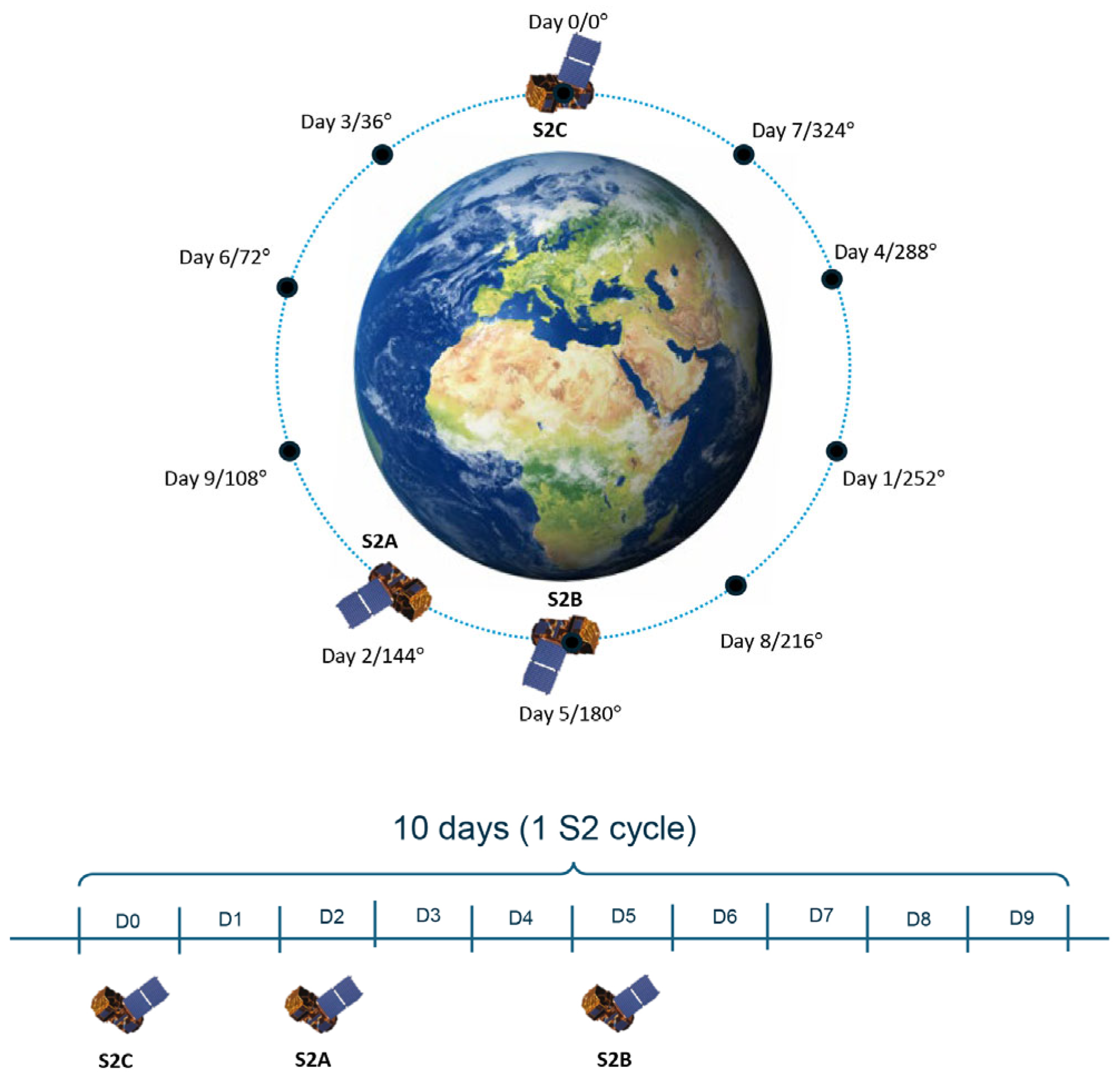
A temporary extension of the Sentinel-2A mission has started in March 2025 to complement the nominal constellation with Sentinel-2B (S2B) and Sentinel-2C. The three-satellite configuration is depicted in Figure 1. The orbital position of Sentinel-2A is such that it can acquire images with nominal viewing conditions 2 days after Sentinel-2C. Sentinel-2A performs systematic acquisitions over Europe and with reduced frequency over the rest of the world.
The present paper reports on radiometric calibration and validation activities performed during the Sentinel-2C commissioning phase. Its first objective is to provide Sentinel-2 users with a status on the mission continuity in terms of radiometric measurements. A second objective is to describe the methodology used to assess absolute and inter-satellite radiometry. With respect to the first two units, two innovations were introduced for the Sentinel-2C commissioning phase: a S2A/S2C tandem formation lasting more than 40 days and Moon acquisitions.

1.2. Sentinel-2C Specific Features

With a few exceptions, Sentinel-2C shares the same design and manufacturing as the previous units. However, from the data quality point of view, it is worth highlighting some specificities [3].
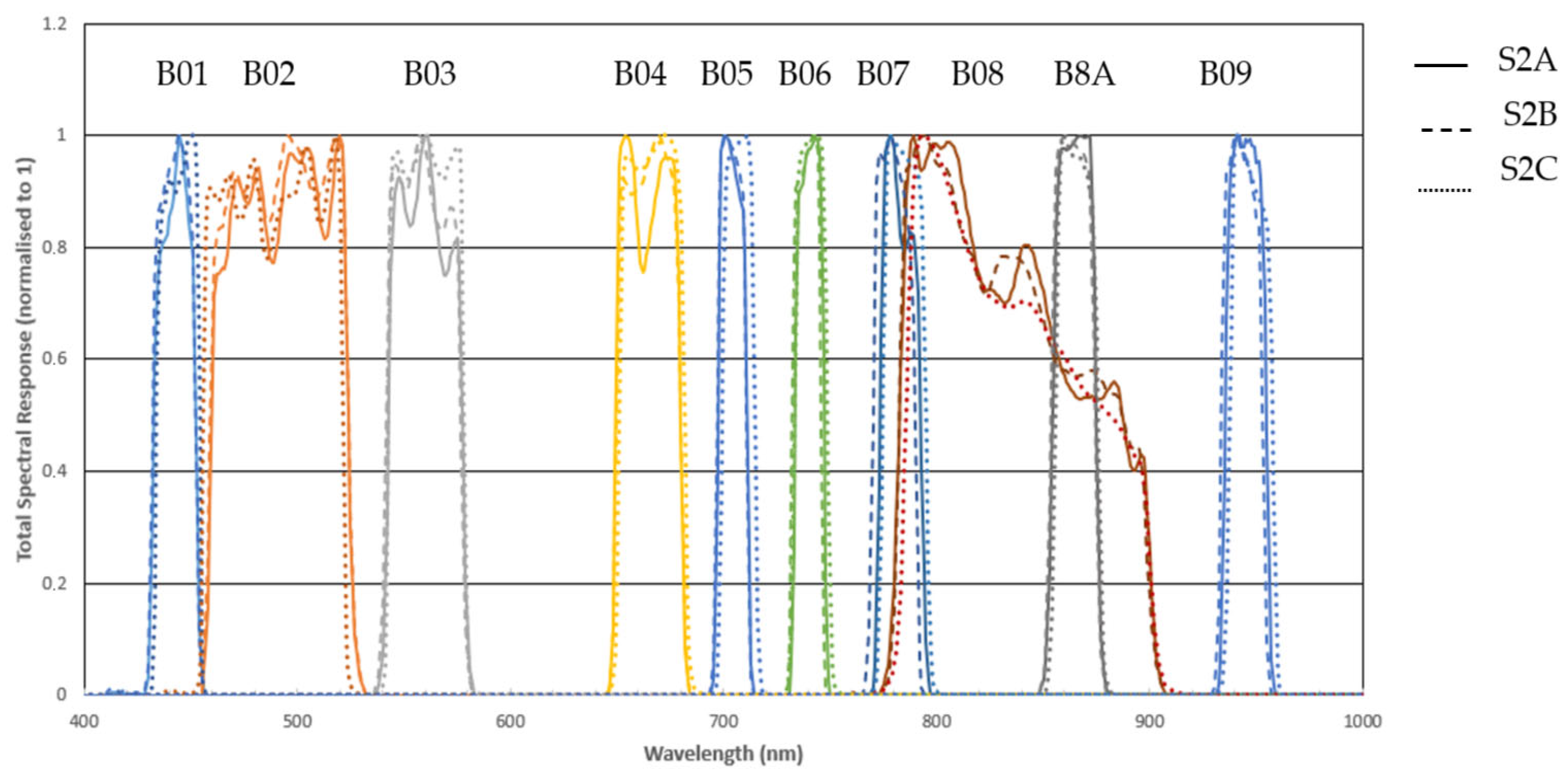
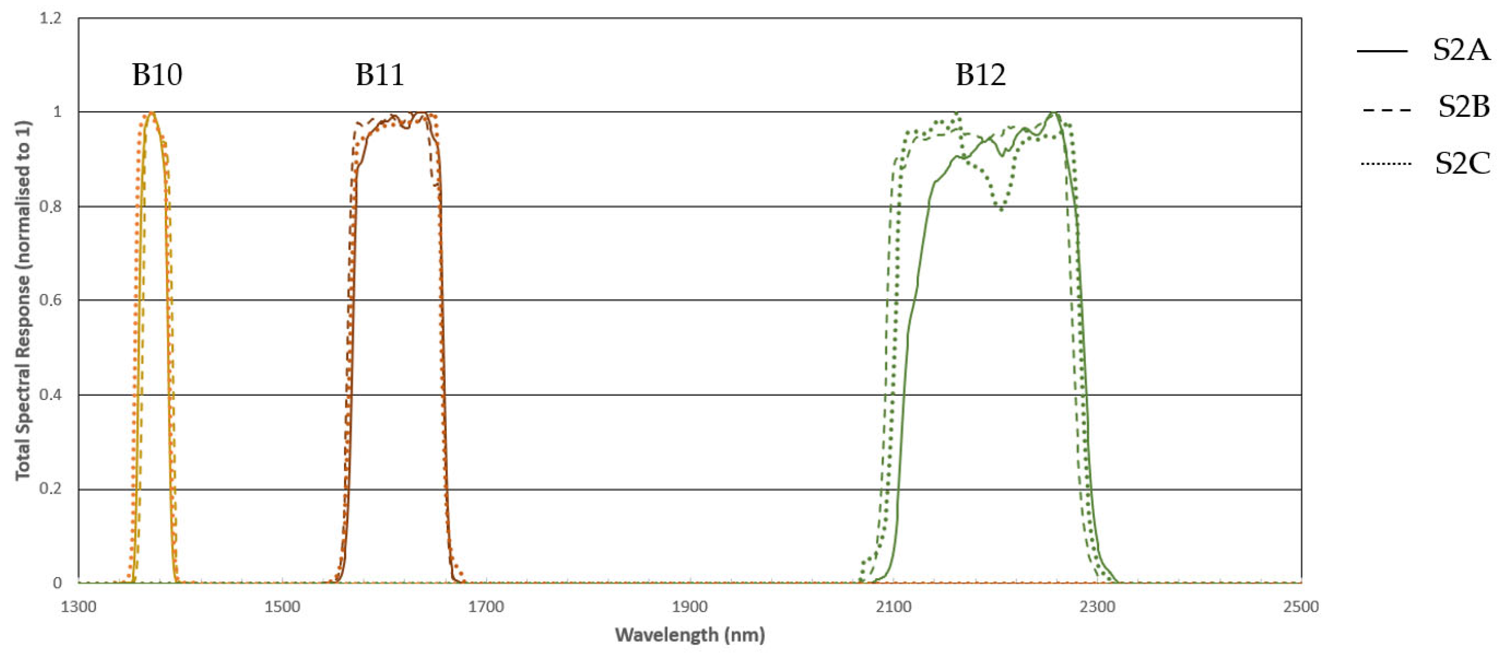
The first specificity concerns differences in relative spectral responses. Although the spectral filters share the same specifications as Sentinel-2A and B, slight variations can be expected. For Sentinel-2C, these differences have been thoroughly characterized on the ground with a per-pixel spectral response measurement [4]. Their impact is analyzed in this paper in Section 5.1. Figure 2 and Figure 3 show respectively the average spectral response functions for the VNIR and SWIR bands of the three units.
Another difference concerns the instrument gains used before analogic to digital conversion. They have been generally increased compared to Sentinel-2A and B models. This results in a higher Signal to Noise Ratio (SNR) for most bands. The SNR performance for the A and B units was already significantly above the specifications, especially for the atmospheric bands (sampled at 60 m). To reflect this situation, the European Space Agency revised upward the SNR requirements (https://sentiwiki.copernicus.eu/web/s2-mission#S2Mission-SpectralResolutionS2-Mission-Spectral-Resolution accessed on 26 April 2026) for the Sentinel-2C and D units.
On the other hand, higher radiometric gains may lead to numerical saturation at a lower radiance level. In practice, this is the case for the cirrus band B10 (at 1375 nm), which can saturate on bright high-altitude clouds more often than for previous units.

1.3. Commissioning Phase Overview

Sentinel-2C was launched on 5 September 2024 and acquired its first image on 17 September. On the 29 October 2024, the satellite started to fly in tandem with Sentinel-2A. The tandem requirements specified an along-track separation below 30 s and an across-track distance below 700 m. Both requirements were successfully met until 11 December 2024, ensuring more than 4 cycles of tandem acquisitions.
On 4 November 2024, a special Sun calibration sequence was performed using different Sun azimuth angles covering in a single day the full range of angles encountered during one year of nominal calibrations, from a specific yaw maneuver. The objective was to improve the Sun diffuser directional response model.
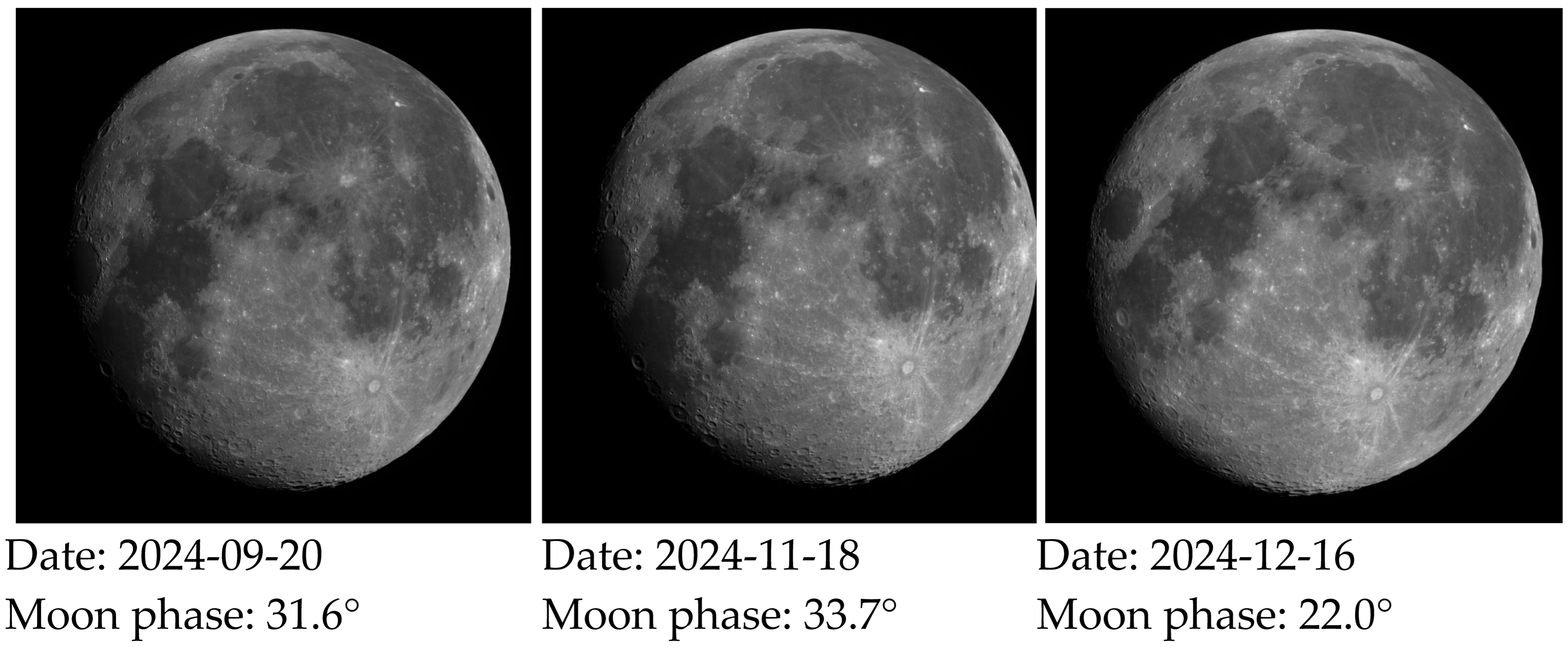
The Moon was also acquired several times during the commissioning phase (September, November and December 2024), with a phase angle close to 30°. The Moon disk was centered on detector 3, and the aspect ratio was close to 11. This was a first for the Sentinel-2 constellation.
Several geometric calibrations were applied to progressively improve the performance, until the mission requirements were met on 9 December 2024.
Sun diffuser calibrations were performed on a bi-monthly basis, and two instrument decontamination operations were conducted during the commissioning phase (the first prior to the sensor start of data acquisitions, the second at the end of November). In parallel, the radiometric performance was monitored using vicarious methods, as described in the following sections of this paper. From this analysis, Sentinel-2C appeared to be somewhat brighter than Sentinel-2A. In order to ensure a continuity of the time series, a radiometric harmonization was decided and implemented on 21 January 2025.
At this date, Sentinel-2C took over Sentinel-2A’s position in the constellation. Sentinel-2A was later moved to a new on-orbit position (see Figure 1) and assigned a temporary mission as a third operational satellite within the constellation, with a reduced acquisition cycle.
Table 2 summarizes the main events of the commissioning phase.

1.4. Article Outline

This article describes the radiometric calibration and validation activities performed during the Sentinel-2C commissioning phase and the main results.
In Section 2, we describe the data and methods used to perform the various activities. We describe the use of the Sun diffuser to carry out radiometric gain calibration and equalization. Absolute and S2A/S2C inter-satellite radiometric validations are performed using Pseudo-Invariant Calibration Sites, lunar acquisitions, Deep Convective Clouds, and pixel-to-pixel comparisons on tandem acquisitions. This section also describes the methodology used to assess the impact of S2A/S2C spectral response differences on typical Earth Observation (EO) scenes.
Section 3 presents the results of the different methods.
In Section 4, we present the S2A/S2C harmonization objectives, approach and implementation. In Section 5, we discuss the robustness and limitations of the results obtained.
In Section 6, we draw some conclusions, lessons learned, and recommendations for future commissioning activities.

2. Material and Methods

2.1. Radiometric Calibration

The MSI is equipped with an on-board Sun diffuser which can be used for absolute calibration. During the commissioning phase, Sun diffuser images were acquired every two weeks approximately to cope with the relatively fast post-launch evolution of instrument radiometric gains, while a single acquisition per month is sufficient for nominal operations. In addition, scenes are acquired at nighttime over ocean for dark signal calibration.
Using the predicted value of the Sun zenith angle on the diffuser, a uniformly illuminated zone is selected from the diffuser image. We then subtract the value of the dark current estimated from dark calibration images. Finally, the corrected signal is compared to the expected value, based on the reflection of the solar irradiance on the sun diffuser, for the Sun–satellite geometry and the diffuser Bi-Directional Reflectance Function (BRDF) characterized on the ground. For a given spectral band, the mean value over all lines and columns provides the estimated instrument gain, while the relative value for each column provides the equalization gain. A complete description of the calibration method is given in [1].
During the S2C commissioning, two different teams applied the same calibration methodology with independent implementation. A close comparison of the results allowed for the identification of minor configuration errors which were subsequently corrected.
In addition, a sequence of Sun acquisitions with different satellite yaw angles was performed on the same day. This maneuver allowed verification of the validity of the Sun diffuser BRDF measured on the ground, as the instrument radiometric response (absolute and equalization gains) should be the same for all acquisitions. The operation was based on a similar activity carried out with Sentinel-3 in 2016, which led to a significant improvement of the OLCI diffuser BRDF model, as reported in [5]. The results for Sentinel-2C highlighted small discrepancies, especially on the edges of the swath. This led to a revision of the S2C diffuser BRDF model which has been deployed in operation since August 2025.
The diffuser image can also be used to analyze the instrument’s random and fixed-pattern noise. The random noise is estimated as the standard deviation along image columns. A two-parameter noise model can be computed using the measured noise at the diffuser radiance and the noise from dark acquisitions. This model can be used to compute the SNR at the reference radiance and compare it with the specifications [6].
The so-called Fixed-Pattern Noise (FPN) is impacted by along-track stripes in the image and results from Pixel Response Non-Uniformity (PRNU) and Dark Signal Non-Uniformity (DSNU). After calibration, both quantities become negligible. The measured value before calibration provides an estimation of the worst-case FPN at the diffuser radiance.

2.2. Radiometric Validation

Radiometric validation activities aim to assess all the radiometric mission requirements such as absolute calibration, the FPN, the cross-calibration with other sensors, the temporal stability, the SNR, the Modulation Transfer Function (MTF) and the spectral consistency. The objective is not only to assess the absolute radiometric performance, but also to ensure the radiometric consistency of the Sentinel-2 constellation.
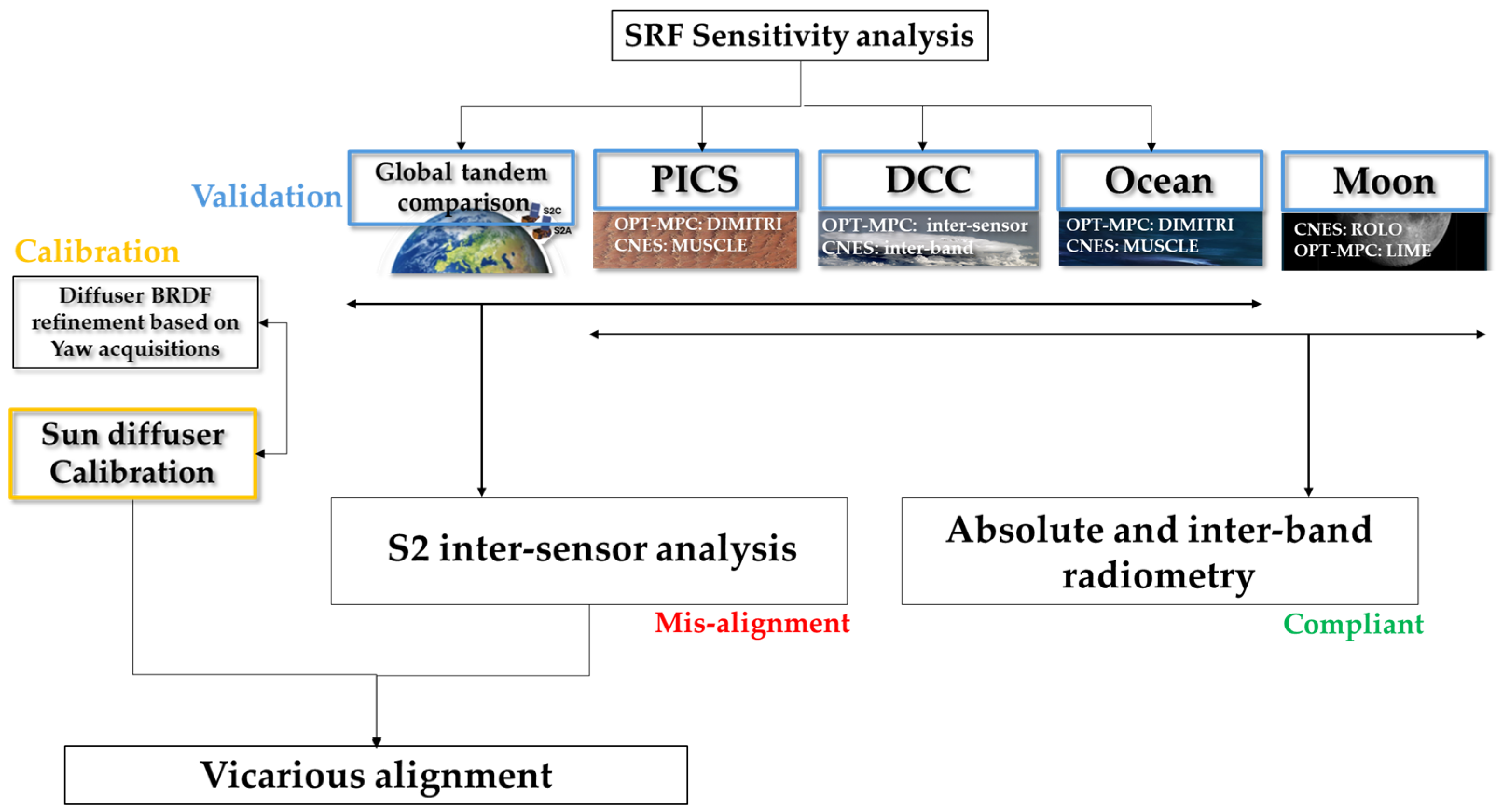
The validation tasks cannot rely on the Sun diffuser images which are already involved in the calibration process (see Section 2.1). Several methods known as vicarious calibration methods can provide an independent estimation of the instrument’s radiometric characteristics based on acquisitions of natural targets. The overall study logic is depicted in Figure 4 below. They were applied to Sentinel-2 by two different teams—i.e., the ESA OPTical Mission Performance Cluster (OPT-MPC) and the French Space Agency (CNES)—to cover all the radiometric aspects. A strong experience of the Sentinel-2 sensor was already gained through the commissioning of the previous two satellite units [7,8,9,10]. In this section, the data and the methods are described.

2.2.1. Vicarious Targets

During the Sentinel-2C commissioning phase, nine targets were analyzed to validate the radiometric quality:
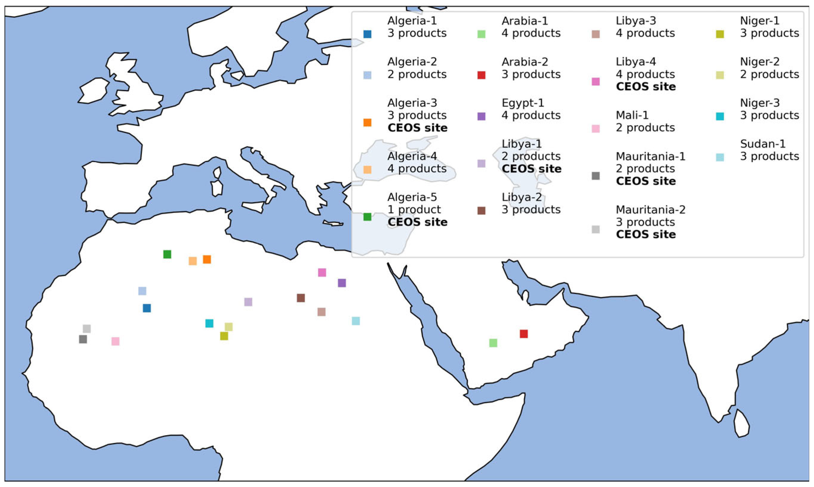
  • Deserts. Also known as Pseudo-Invariant Calibration Sites (PICSs), desert sites are rather stable over time (very few to no vegetation, nor human activity), giving a perfect target to compare multiple images together. Either several images from the same sensor can be compared together for multi-temporal monitoring or several images from various sensors can be compared for cross-calibration. The latter analysis requires a standardization of the PICS footprints among the missions. Back in 1996, CNES has proposed a first selection of 20 desert sites [11]. In 2008, CEOS-IVOS endorsed six of them, which were then adopted by the OPT-MPC. The present study is mainly based on the small sites, around 20 km × 20 km, whose locations are given in Figure 5.
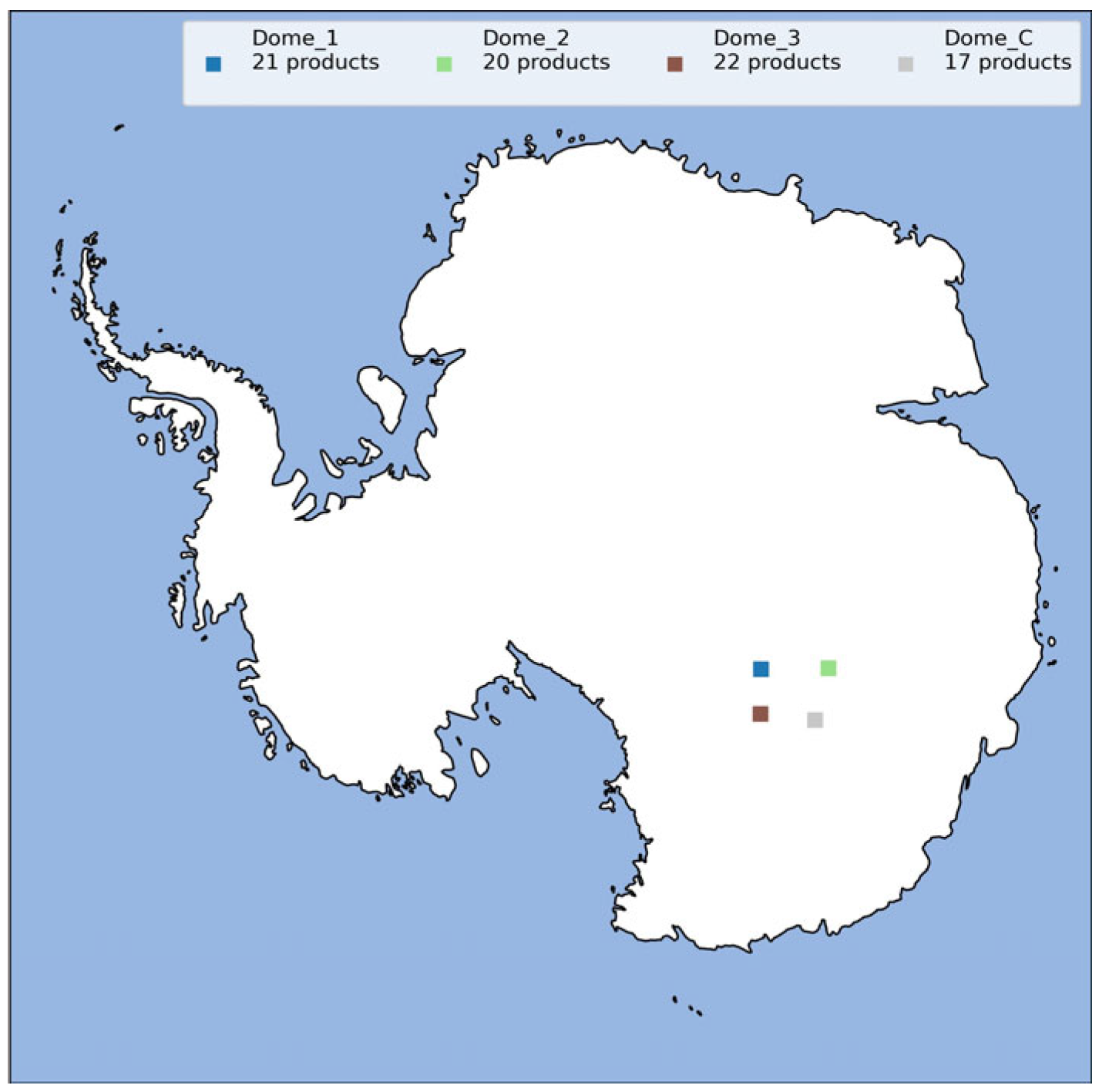
  • Domes. Located in Antarctica, the dome sites offer the same stability as the desert sites but in a very cold environment. They can be considered as PICSs [12]. Four 100 km × 100 km footprints were selected by CNES around the Concordia station, including the Dome-C site now endorsed by CEOS [13]. The geographic positions are displayed in Figure 6.
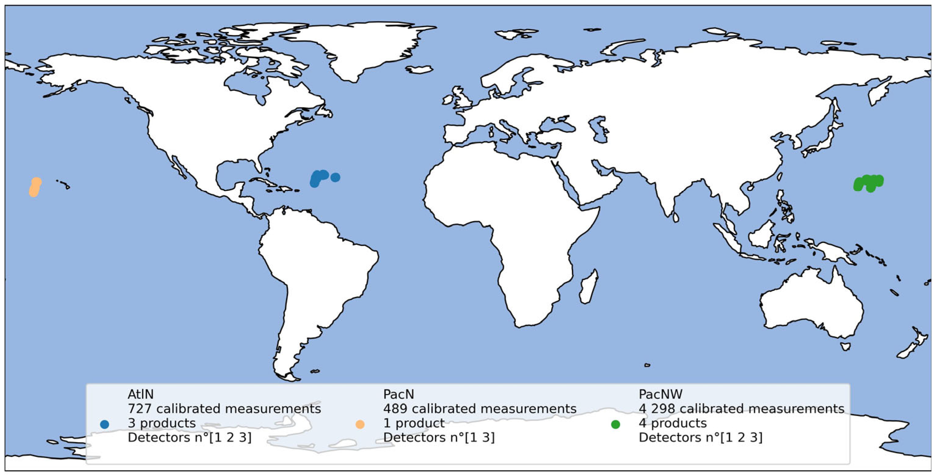
  • Ocean. Over ocean, for the short wavelengths, the signal acquired by the satellite is mainly due to the molecular scattering in the atmosphere. This phenomenon—also known as Rayleigh scattering—can be accurately simulated by a radiative transfer model and compared to acquisitions to estimate the absolute calibration. This method requires selecting images in which the Rayleigh contribution is maximized and the marine reflectance is minimized. Based on a SeaWiFS climatology and GlobColour climatology, six oligotrophic areas were selected for their spatial and temporal stability associated with a low surface reflectance due to low phytoplankton and sediment concentrations [6,7,14,15]. Figure 7 shows where the datasets are collected.
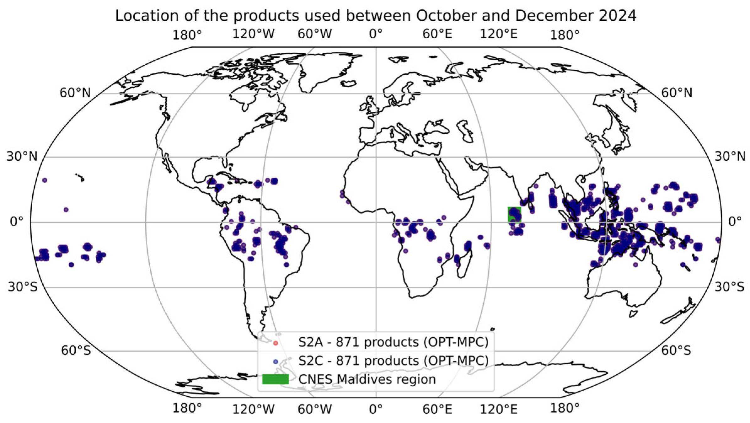
  • Deep Convective Clouds. This cloud type can be used as spectrally, spatially and temporally stable targets (at least up to about 800 nm). These clouds occur frequently in the Tropics. Moreover, their top reaches the tropopause at about 16 km and they span over large areas, making them good targets for satellite cross-comparisons as they are easy to spot and only small atmospheric corrections need to be performed. Their spectral reflectance can also be simulated by a radiative transfer model for wavelengths up to 800 nm to derive an inter-band calibration. Between October and December 2024, about 900 DCC tandem products acquired by both Sentinel-2A and Sentinel-2C have been found. The geographical location of these products across the globe is presented in Figure 8. The satellite cross-comparison performed by OPT-MPC is computed using all available DCCs, ensuring that the statistics cover all conditions. Regarding the inter-band calibration based on simulations, CNES focuses on the Maldives region because DCCs over open ocean should be closer to the theoretical DCC model used. In addition, time series of calibration results are available on this region since the Sentinel-2A commissioning phase (2015).
  • Moon. For the first time on a Sentinel-2 instrument, the Moon was acquired during the commissioning phase. Three images were available, always on detector 3. The maneuver induced an acquisition slow-down which distorts the Moon: the along-track direction is stretched by a factor close to 11 compared to the across-track direction. The quick-looks presented in Figure 9 are corrected from this geometrical distortion.
  • Global Earth Per-Pixel Tandem Data. In order to analyze the discrepancies between Sentinel-2C and Sentinel-2A, the study has highly benefited from the satellite tandem configuration described in Section 1.3. In this case, the vicarious targets were acquired quasi-simultaneously—around 30 s apart—and with the same acquisition geometry between the two satellites. This specific maneuver was motivated by the Sentinel-3B commissioning phase (in 2018) during which a tandem phase with Sentinel-3A had proven large benefits [16].

2.2.2. PICS Processing Tools

Two different approaches are applied to the Sentinel-2C images. The OPT-MPC analyses are based on the DIMITRI (Database for Imaging Multi-Spectral Instruments and Tools for Radiometric Intercomparison) tool whereas CNES relies on SADE/MUSCLE (MUlti Sensor CaLibration Environment):
  • DIMITRI. The algorithm aims to simulate the top-of-atmosphere (TOA) reflectance in the visible to near-infrared (VNIR) spectral range over pre-defined sites. The first step of this method consists of building a reference surface reflectance model for the selected site followed by model calibration using TOA measurements from a reference sensor (MERIS in DIMITRI). TOA measurements are propagated to the surface using an inverse radiative transfer simulation. A database of bottom-of-atmosphere (BOA) measurements with various acquisition geometries (solar and viewing zenith angles and relative azimuth angles) is built. The database is used to fit a four-parameter BRDF model (for each spectral band). A hyperspectral model is constructed using spectral interpolation [17].
    The second step consists of the simulation of the TOA reflectance signal using the reference BRDF model and considering the observation geometry (e.g., MSI-C). Ozone and water vapor content are retrieved from the European Centre for Medium-range for Weather Forecasts (ECMWF), while a constant aerosol optical thickness is assumed [18]. The resulting hyperspectral signal is then convolved with the spectral response of the instrument to produce the simulated TOA reflectance of the sensor under test (e.g., MSI-C). The method has been used to assess the radiometry of Sentinel-2C/MSI relative to the reference sensor (MERIS for DIMITRI) or relative to Sentinel-2A/MSI using a double ratio [1,19].
    More than 38 S2C Level-1C (cloud-free) products have been successfully retrieved over CEOS desert test sites (Algeria-3 and Algeria-5, Libya-1 and Libya-4, Mauritania-1 and Mauritania-2—see Figure 5 for site location).
    The PICS method implemented in DIMITRI can be used to compare measurements of individual sensors to the reference (MERIS) or to inter-compare measurements of different sensors with comparable spectral bands using the double ratio technique [19].
  • SADE/MUSCLE. CNES has been gathering all the vicarious calibration methods into this tool for more than 20 years. The MUSCLE software implements calibration algorithms with a generic approach, applicable to any satellites. SADE (Structure d’Accueil des Données d’Etalonnage) is the database which collects a very large amount of vicarious calibration data from a very large number of sensors [20,21]. The SADE/MUSCLE version 11.11.0 is used in this study. At the time of writing, about 33 million measurements from 49 sensors are available, including mean reflectance over predefined areas such as PICSs, the standard deviation, the acquisition angular conditions, the acquisition timestamp and auxiliary data about the atmosphere. Sharing a generic tool among all satellites grants that calibration results are comparable whatever the sensors and offers the possibility of extensive cross-comparisons, helping end users to combine data from various missions.
    Among the available methods, the PICS method is applicable both to the desert and dome sites mentioned in Section 2.2.1. The data extraction—consisting of averaging the Sentinel-2 image over the predefined PICS footprint—is handled by S2ETRAC (Sentinel-2 Extraction Tool for Radiometric Analysis and Calibration) operated by OPT-MPC before insertion into SADE/MUSCLE.
    The implemented PICS approach is based on a measurement comparison, in our case, a comparison between Sentinel-2C and another sensor taken as reference such as Sentinel-3 OLCI-B, LANDSAT-9, etc. This comparison should not be biased by any directional effects, so the first step is to pair up the measurements for which the angular conditions match. Then, for each measurement pairs, an atmospheric correction—based on SMAC [22]—is applied to take into account the atmospheric variations which may occur between the two measurements. Finally, the spectral response discrepancies between the two sensors under comparison are taken into account. For more details, readers can refer to [23,24].
    This approach is applicable over the entire reflective spectral domain, providing the sensor taken as reference is covering the spectral range of interest. Only the atmospheric absorption bands cannot be calibrated. CNES has applied this technique to monitor the radiometry of a large number of satellites including MERIS [25], PLEIADES [26], PRISMA [27], Sentinel-3 [28,29], Sentinel-2 [30], the SPOT missions [31] and VENµS [32].
    For domes, the SWIR range is not available because, over this spectral range, the snow microstructure modifies the ground reflectance, and the site is not stable anymore over time.

2.2.3. Ocean Processing Tools

As for PICSs, the ocean analysis relies on two independent implementations, one from OPT-MPC, the other from CNES:
  • DIMITRI. The Rayleigh scattering algorithm is based on the methodology of [33,34] using open ocean observations, to simulate the molecular scattering (Rayleigh) in the visible domain and comparing against the observed TOA reflectance to derive a calibration gain coefficient.
    To ensure a proper computation of the vicarious coefficients over Rayleigh scattering, the following conditions need to be satisfied: (1) <1% cloud coverage on ROI; (2) low wind speed, typically less than 5 m/s; and (3) low content of aerosol. The cloud screening employs a specific algorithm using two band ratios (red-edge1/NIR and blue/red-edge2) [35,36].
    The marine reflectance is computed using a marine model following [37,38].
    Following the ingestion of L1C data, including cloud screening, TOA reflectance, and solar and viewing angles, the cloud mask and auxiliary variables are stored on a per-pixel basis. Quick-looks for each acquisition are generated [39]. This approach is applicable up to 700 nm, above which the Rayleigh scattering contribution decreases significantly in the acquired signal.
  • SADE/MUSCLE. The ocean method is part of the SADE/MUSCLE environment developed in CNES as already described in Section 2.2.2. As for PICS, the input data are produced by S2ETRAC. In this case, the averaging is applied on clear-sky 960 m × 960 m image subsets. For each subset, a radiative transfer model estimates the theoretical signal which should have been acquired by the satellite. The ratio between the measurement and the theory gives the calibration ratio.
    The theoretical signal computation relies on the SMAC radiative transfer code [22] to enable very fast computations of gaseous transmission whereas SOS [40] is preferred for aerosol and molecular diffusion computations. The atmospheric conditions, especially the surface pressure, the surface wind speed and the ozone content, are taken from ECMWF. The aerosol content is derived from the optical thickness observed at 865 nm (band B8A) and the aerosol type is taken as a maritime model with 98% of relative humidity (M98 model) [41]. The marine reflectance contribution is estimated from a SeaWIFS climatology [14]. Only the main implementation characteristics are recalled here, essentially to spot the differences among the tools; but more details can be found in [33,42].
    The method uncertainty increases with wavelength above 800 nm, as Rayleigh scattering is no longer the main contributor to the acquired signal. The ocean measurements of various sensors such as MERIS [25], PARASOL [43], PLEIADES [44], POLDER [33], Sentinel-2 [30], Sentinel-3 [28,29], and SPOT4 [45] were analyzed with this tool.

2.2.4. Deep Convective Clouds Processing Tools

The DCC images are studied with two different tools targeting two different objectives. The first one cross-compares two satellites, the second one compares the spectral bands within a given satellite, also known as inter-band calibration:
  • OPT-MPC. DCCs have been used to inter-compare Sentinel-2A and Sentinel-2C during the tandem phase, using the method presented in [46] which is summarized hereafter. This method was developed more than twenty years ago, and was first described in [47,48].
    DCCs are detected in MSI level 1 images using thresholds on bands 8A and 10 (at 865 nm and 1375 nm) in every scene acquired between −20° and 20° of latitude. If the cloud is of sufficient size, atmospheric correction is applied and DCC pixels are accumulated to build a histogram per band and per month. A skewed Gaussian curve is fitted to the histogram and the second inflexion point of the distribution is used as the reflectance indicator for the distribution. The bootstrap method is used to estimate the standard deviation of the reflectance indicator. This reflectance indicator is estimated for various sensors. The resulting estimates are then compared for the corresponding bands, after correction for differences in the spectral response functions using spectral band adjustment factors. These adjustment factors have been computed using EnMAP [49] hyperspectral acquisitions of DCC; the uncertainty associated with these adjustment factors is the variability in the DCC radiometry among the hyperspectral acquisitions. The uncertainty associated with each reflectance indicator is computed using both the spread of the results from the bootstrap method and the uncertainty of the spectral band adjustment factors. Results for band 10 at 1375 nm are not presented as this band saturates in very bright environments at different values for MSI-A and MSI-C. A DCC signal above 800 nm tends to vary depending on the particle properties of each cloud. However, as this method is statistical and uses a great number of products, DCC properties above 800 nm tend to average to a “mean cloud” and thus can be compared between sensors after applying spectral band adjustment factors.
  • SADE/MUSCLE. The DCC method which is included in SADE/MUSCLE (cf. Section 2.2.2) is dedicated to inter-band calibration. As for the ocean sites, the data extraction is handled by S2ETRAC, averaging the image over 960 m × 960 m subsets. The DCC identification follows the same thresholding strategy as that described in the previous bullet point. Due to the Sentinel-2C specificities (cf. Section 1.2), saturation may occur over DCC. For each subset, the theoretical spectral shape of the signal is computed by a radiative transfer model based on the atmospheric conditions given by ECMWF. The simulation does not provide an accurate absolute level, so a band measurement is taken as reference to set the absolute level. On Sentinel-2, the band B4 (665 nm) is taken as reference. If the absolute level is very different from the expectations, then the result is considered as out-of-range with regard to the simulation hypothesis and discarded. The inter-band results are given as the ratio between the measurement and the simulation, assuming that B4 is perfectly calibrated.
    As for the ocean method, the SMAC radiative transfer code [22] is in charge of the gaseous transmission. SOS [40] is used to simulate the DCC signal based on an averaged DCC structure. Above 800 nm, the signal is more and more dependant on the particle microstructure on top of the DCC, which is unknown, and the simulation becomes unreliable. Therefore, the method cannot by applied for large wavelengths. The full method description is available in [50]. CNES has applied this approach to several sensors such as PARASOL [43], POLDER [33], Sentinel-2 [30] and Sentinel-3 [28].

2.2.5. Moon Processing

The Moon images have two main advantages. First, the image offers a very strong contrast between the bright Moon and the dark background. This contrast can reveal various image artifacts such as straylight effects and can help to quantify them. Second, the Moon’s surface is very stable over time and the measured irradiance can be compared to a lunar irradiance model to perform calibration. In this paper, we focus on the second aspect.
To compute the lunar irradiance, the instantaneous field of view (IFOV) of all pixels in the Moon acquisition should be computed. While the across-track dimension depends only on the instrument characteristics, the along-track dimension depends on the sweep rate during the acquisition, which is responsible for the strong distortion of the Moon disk in the images. The IFOVs are computed by OPT-MPC based on the Attitude and Orbit Control System (AOCS) and the pixel viewing directions. Once the lunar irradiance is computed, it can be compared to a reference model which takes into account the Sun–Moon–satellite geometry (distance, phase angle and libration parameters) and the instrument’s spectral response. Two different models are used in the present work:
  • LIME-ESA. The Lunar Irradiance Model of ESA (LIME) [51] delivers an SI-traceable reference of the Moon’s disk-integrated irradiance, designed for the radiometric calibration of Earth Observation sensors. It is based on over 590 nights of lunar observations with a Cimel CE318-TP9 photometer at the Izaña Observatory and Teide Peak in Tenerife. The instrument was calibrated at the National Physical Laboratory to characterize responsivity, linearity, and temperature effects. Top-of-atmosphere irradiance is retrieved through Langley plot methods, eliminating atmospheric contributions. The model uses a wavelength-dependent parametric formulation to describe irradiance variations with lunar phase and libration geometry. LIME achieves uncertainties of around 2% across most spectral channels and shows strong agreement with satellite lunar acquisitions, enabling improved calibration accuracy and sensor stability monitoring.
  • ROLO-CNES. The Robotic Lunar Observatory (ROLO) from USGS in Flagstaff, Arizona, has systematically acquired the lunar irradiance for 3 years with a 32-spectral-band instrument ranging from 347 nm up to 2390 nm. This dataset was then fitted by a model called ROLO [52]. In 2017, CNES has applied this model to 1435 images of the Moon acquired by PLEIADES satellites and has published a ROLO-CNES correction to improve the absolute radiometry and the modeling of the Moon phase angle dependency [53]. As PLEIADES is a sensor restricted to the VNIR range, the associated corrections are only valid in this spectral range. The corrected model provide a 3% absolute calibration accuracy. Regarding the multi-temporal calibration, a 1% accuracy can be obtained.
Unfortunately, lunar calibration could not be used for S2A/S2C cross-calibration as no Sentinel-2A lunar acquisition was available. Such a cross-comparison would be achievable within the Copernicus missions between Sentinel-2 C and Sentinel-3 OLCI-B because Sentinel-3 B also acquired the Moon during its commissioning phase [54].

2.2.6. Global Earth Tandem Analysis Processing Tools

This methodology relies on the direct pixel-to-pixel comparison of data acquired during the tandem phase, considering that differences in atmospheric and geometric viewing conditions have a negligible impact. The large number of measurements available allow us to analyze the impacts of several parameters on the inter-satellite differences: type of scene, radiance level, and position in the field of view.
The initial dataset is composed of a S2A-S2C pair of images with less than 1% cloud coverage and refined geometry. In addition, we apply a filtering on the type of scene, according to the L2A scene classification layer: separate statistics for bare soil, vegetation and water pixels are generated, while other pixels are discarded from the analysis. This allows us to assess the impact of differences in spectral response, since no spectral adjustment is performed for this method.
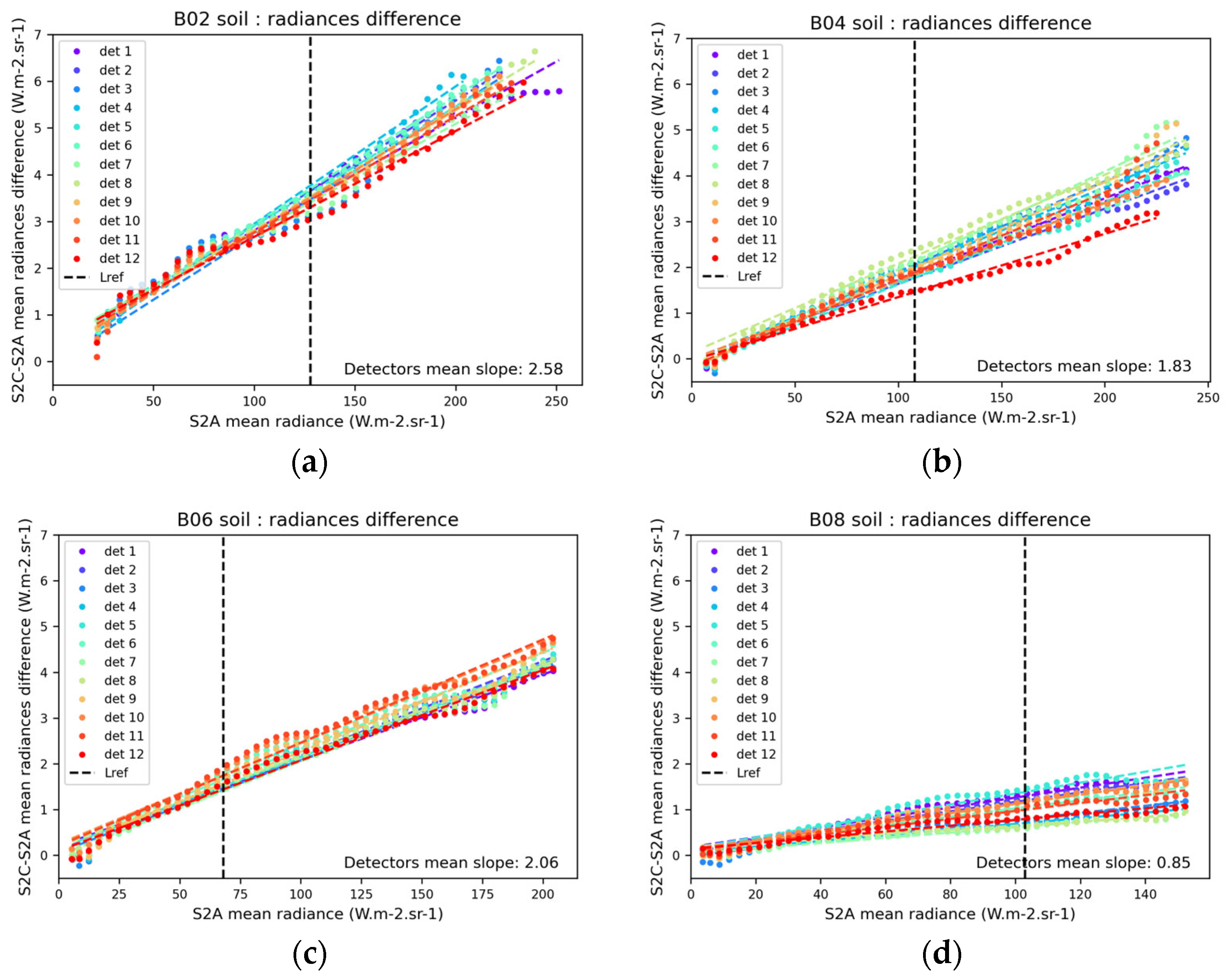
The reflectance measurements are converted to radiance. 2D histograms of radiance difference (S2C − S2A) vs. S2A radiance are generated for each spectral band and detector, as illustrated in Figure 10 below. Such figures were used to check for the presence of unexpected offsets, non-linear effects or strong inter-detector variations. The best estimate of the linear gains is then computed. The analysis is repeated for three periods to assess the temporal stability of the results:
  • From 1 to 6 November 2024: 506 tiles;
  • From 7 to 13 November 2024: 558 tiles;
  • From 14 to 20 November 2024: 647 tiles.

3. Results

3.1. Radiometric Calibration Results

As mentioned in Section 2.1, couples of dark and Sun diffuser acquisitions are used to process nominal calibration. The dark coefficients are updated and used to correct the Sun diffuser images. A decontamination of the Sentinel-2C instrument was carried out from 25 November 12:20 UTC to 26 November 16:20 UTC 2024.

3.1.1. Absolute Gains

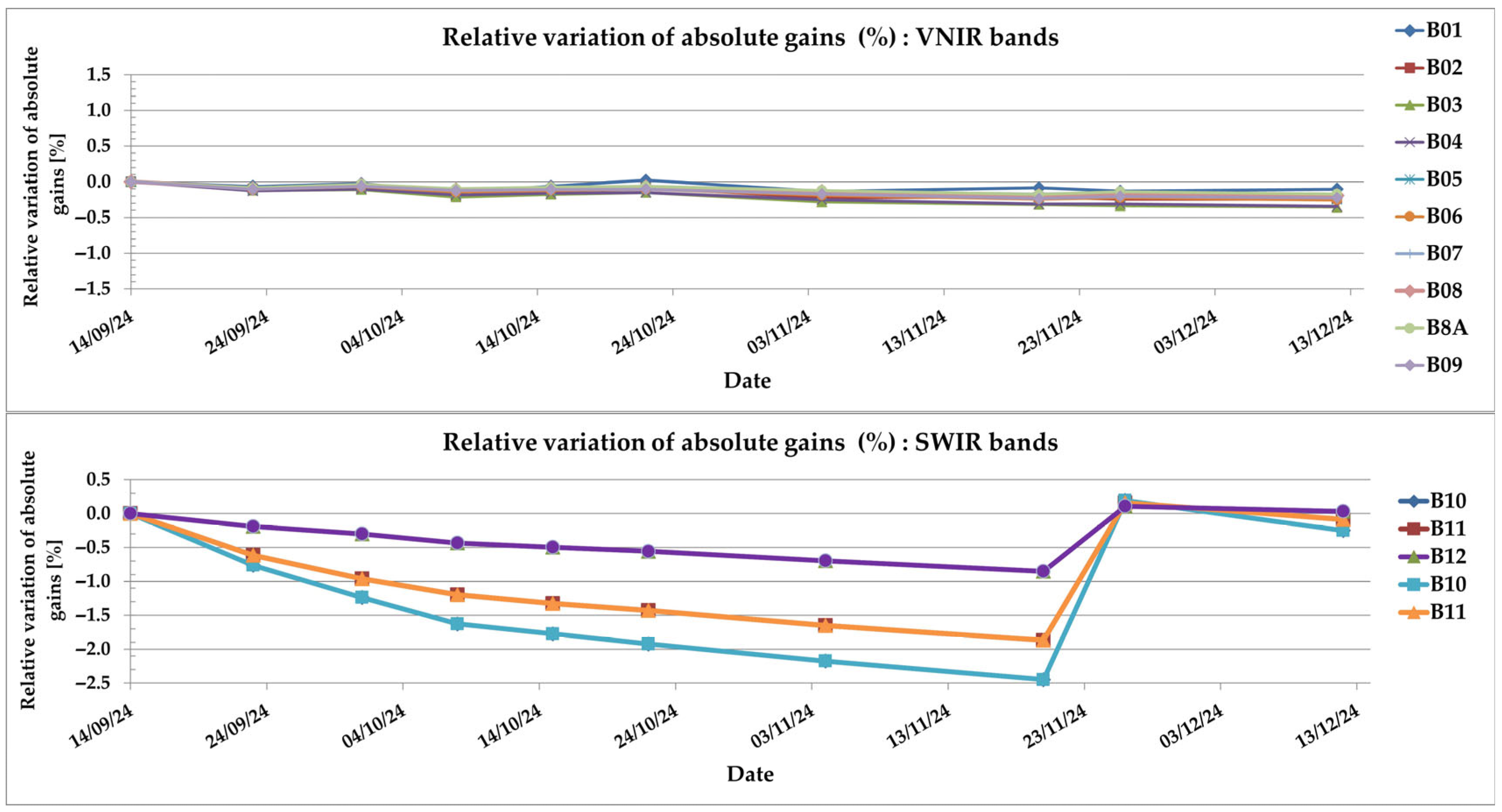
The changes in absolute gains over time are illustrated in Figure 11, with respect to the first in-flight calibration on 14 September 2024.
For VNIR bands, Sun diffuser calibrations show a sensitivity loss in-flight from 14 September 2024, the first in-flight calibration, to 12 December 2024, the last calibration performed during the S2C commissioning, by about 0.10 to 0.35%. The lowest decrease is obtained for the B01 band. We note the steady loss of sensitivity is punctuated by small fluctuations (often lower than 0.05%). OPT-MPC had also observed fluctuations in absolute gains for MSI-A and MSI-B and for OLCI too for few months. These were probably due to fluctuations in solar irradiance relative to its maximum activity.
For the SWIR bands, we observe a faster decrease in sensitivity over time. While the slope per band was the most important at the beginning of the mission, it gradually showed a smaller decrease over time. This behavior is expected, as it results from ice deposition on the sensor optics (caused by a tiny amount of water vapor trapped in the instrument) for which the SWIR bands are sensitive. Between the first in-flight calibration from 14 September to 20 November, the impact is the most important for the B10 band (−2.5%), then the B11 band (−1.9%), and finally B12 (−0.9%). Regular calibrations allow the monitoring of sensitivity changes and updates of the absolute gains accordingly, to ensure the continued accuracy of the provided reflectance data. Moreover, the decontamination carried out between 25 and 26 November 2024 restored the sensitivity of the SWIR bands to their initial levels.

3.1.2. Equalization Gains

The stability in equalization coefficients is given by the Ra factor, which expresses the relative change between updated coefficients and reference coefficients. A complete mathematical expression of this parameter is defined in [1]. Basically, if we consider the cubic model of non-linearity and equalization used for the VNIR bands, the relation between the equalized measurements Z m e a s b , d , l , p and the measurements corrected for the dark signal Y m e a s b , d , l , p , in digital counts, is:
Z m e a s b , d , l , p = n = 1 3 G n b , d , p × Y m e a s n b , d , l , p
where b, d, l , p are respectively indices for band, detector, line and pixel.
The Ra factor is used in the update of the coefficients G n of the model as follows:
G n u p d a t e d b , d , p = G n c u r r e n t b , d , p × R a n b , d , p
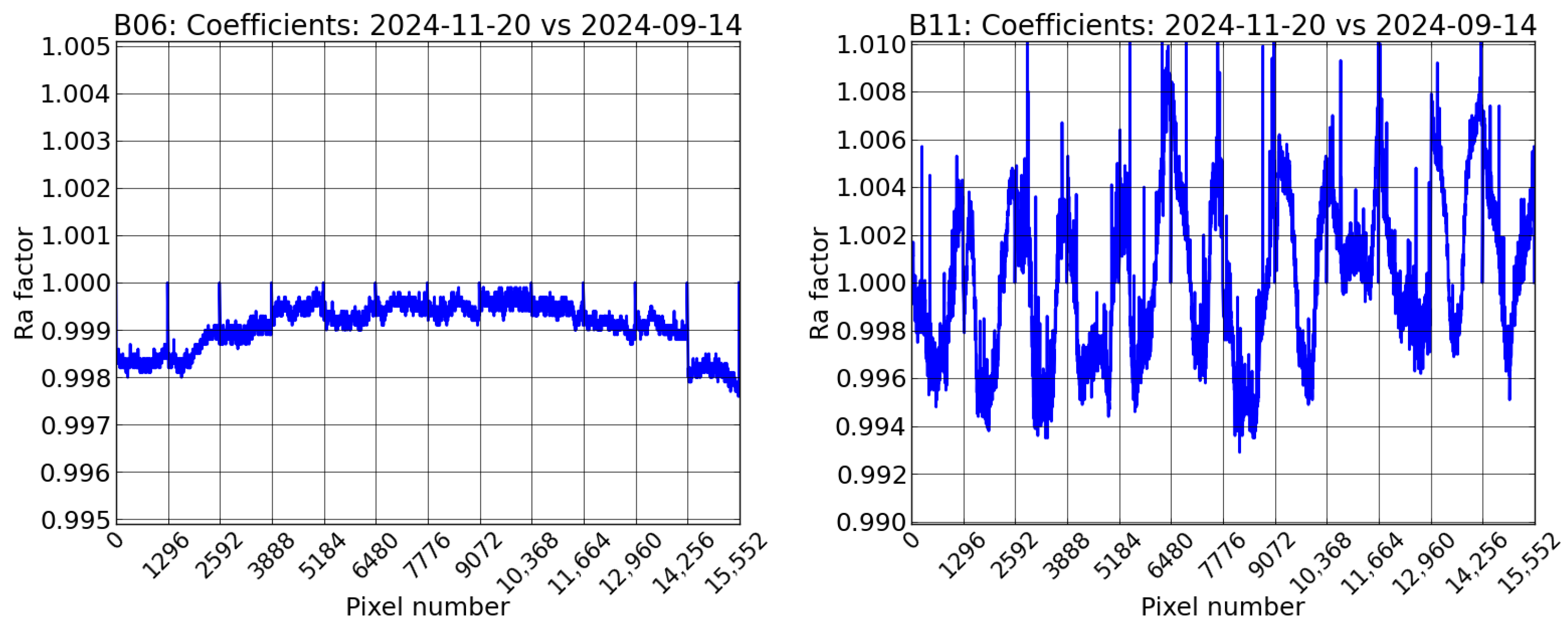
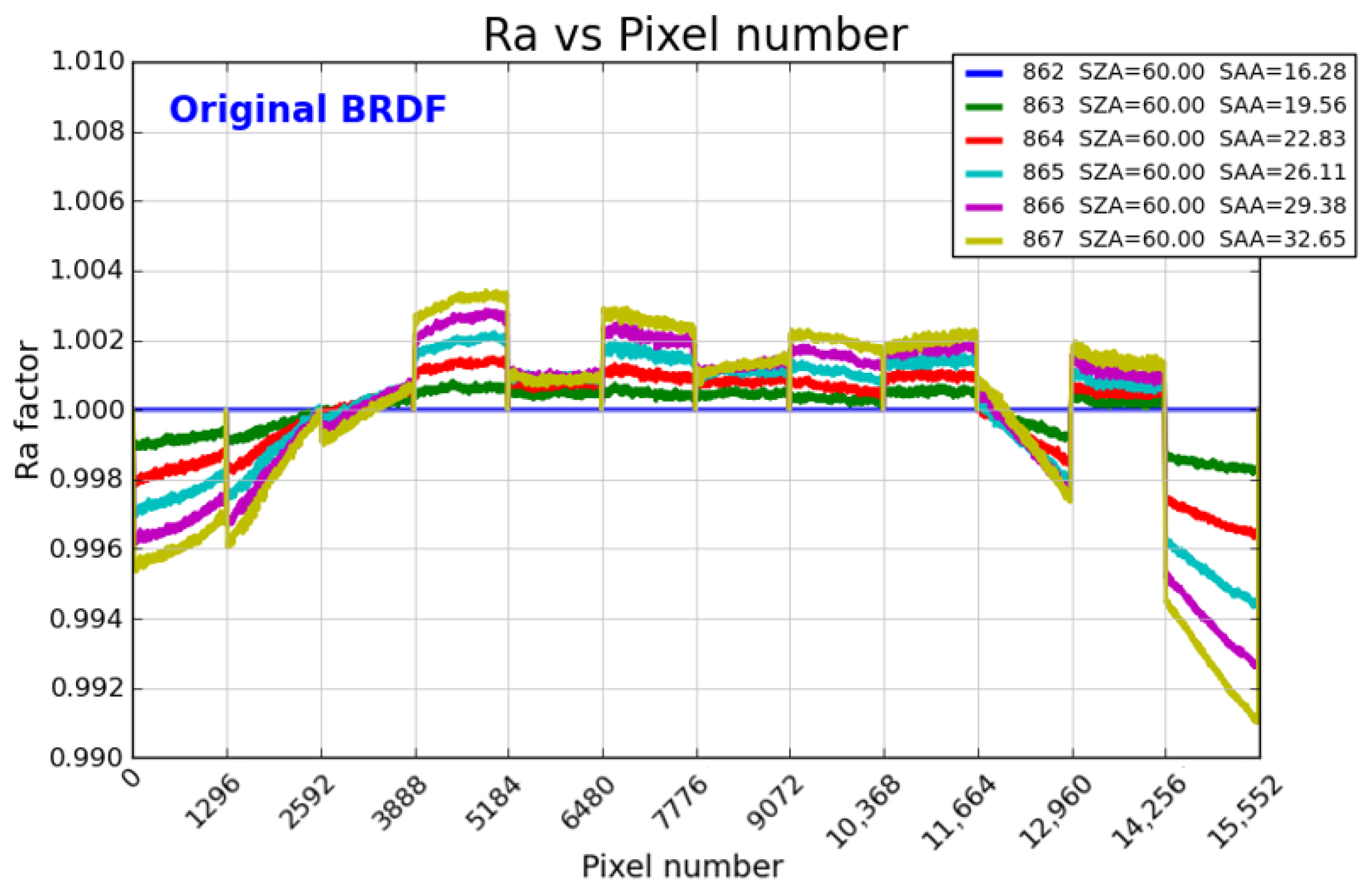
If we consider the change in equalization coefficients between the first in-flight assessment (based on the Sun product acquired on 14 September) and the Sun acquisition on 20 November (the last acquisition before the decontamination), we can see in Table 3 that there is no more than 0.2% of extreme variation for most of the VNIR bands (only the B09 band has a maximum variation of 0.3%). Moreover, the very small standard deviation of the Ra factor, which is lower than 0.05% for the VNIR bands, highlights that the extreme variations are located in a few pixels, while most of them have no change in their inter-pixel response. Figure 12 illustrates this great stability for the B06 band (left illustration): the y-axis range extends across 1%, while the variation in equalization coefficients is limited to a range of 0.2%. The grid on the x-axis shows the limits of the 12 detectors. The Ra factor is 1 at the edge of the detectors: indeed, these pixels are blind pixels (unilluminated) for which it is not possible to update the equalization coefficients in flight.
The variations are higher for the SWIR bands and affect most of the pixels, with extreme variations in a few percents (here 1% in B12, 3% in B10), as usually seen for MSI-A and MSI-B. Figure 11 illustrates these variations for the B11 band (right illustration).
Sun diffuser acquisitions during the in-orbit commissioning were acquired with very similar incidence angles. As a result, the reflectance of the Sun diffuser has always been the same.
But, over a complete yearly cycle of Sun acquisitions, there is a variation in the incidence angle which leads to a change in the used value of the Sun diffuser BRDF. Consequently, slight inaccuracies in the BRDF characterization can affect the equalization coefficients. Such defaults have been characterized during the in-orbit commissioning phase of MSI-C, from a yaw maneuver carried out on 4 November 2024 which enabled the acquisition of six successive Sun diffuser measurements for different Sun incidences representative of angular variations over a year. This effect is illustrated in Figure 13 for the B01 band. One can see that edge detectors (D1 on the left part, D12 on the right part) have the highest variations introduced in the equalization coefficients of up to 0.9%.
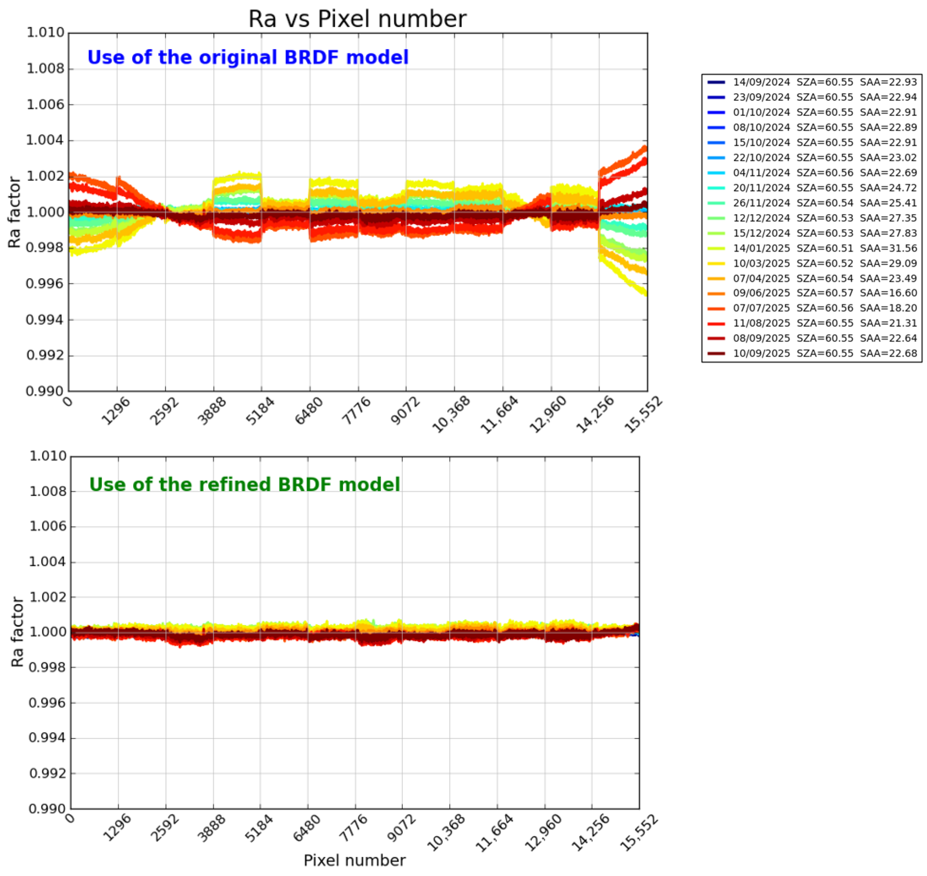
These variations are unexpected from successive Sun diffuser acquisitions. Indeed, they do not correspond to a real change in the sensor response but highlight slight defects in the Sun diffuser BRDF characterization. Therefore, they could be used to refine the Sun diffuser BRDF characterization. The resulting refined BRDF was then evaluated on time series of Sun diffuser acquisitions over the first year in flight: from the very first one (on 14 September 2024) to the Sun acquisition on 10 September 2025. As an example, Figure 14 shows the estimation of changes in equalization coefficients for band B01 when using the original BRDF and when using the refined BRDF. The benefit of the BRDF refinement appears clearly: the stability of equalization is strongly improved, and variations over time no longer exist.

3.1.3. Identification of Defective Pixels

Based on the analysis of the SNR, the commissioning phase also revealed a few defective pixels: three pixels in band B11 and one pixel in band B12. Their measurements are not used to produce L1C images, but they are interpolated from neighboring pixels and flagged in the image quality masks.

3.2. Radiometric Validation Results

In this section, the validation results are expressed as the ratio Δ A k between the measurement made by the sensor to calibrate and the reference measurement (which can come from a reference sensor or a simulation depending on the method) for each spectral band k .

3.2.1. Cross-Comparison on PICSs

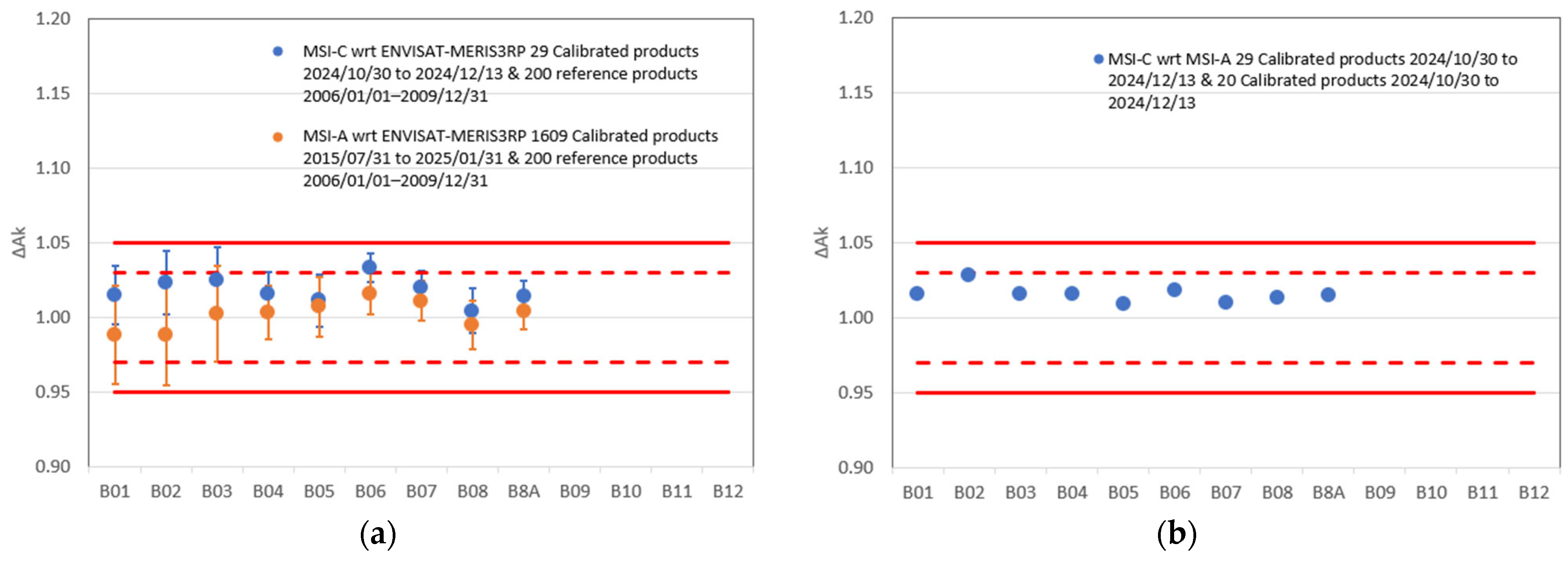
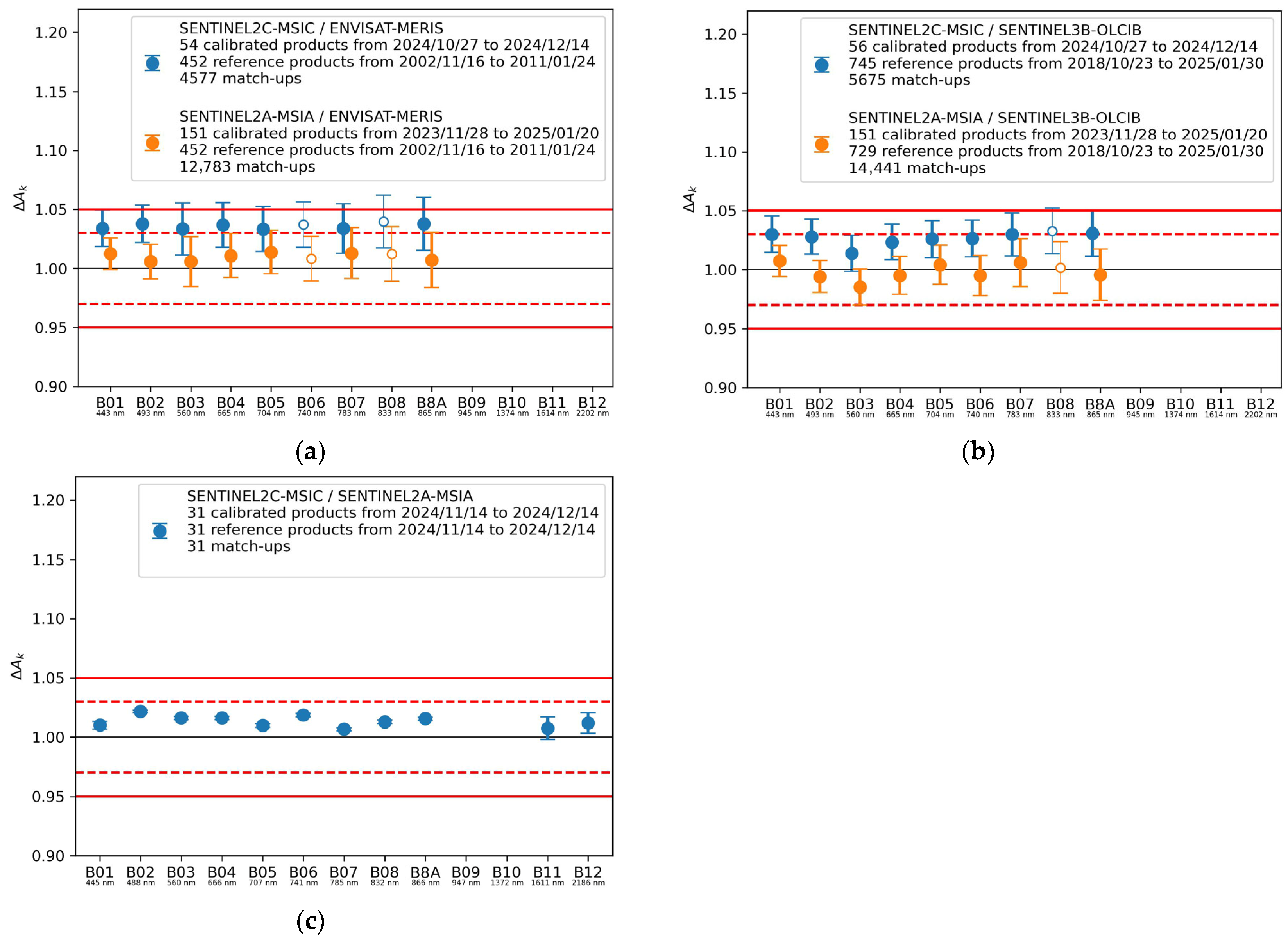
The DIMITRI cross-calibration results over desert sites are provided in Figure 15 using the ENVISAT-MERIS 3rd Reprocessing dataset as a reference sensor and using the double ratio technique with regard to Sentinel-2A-MSI (Figure 15a and Figure 15b respectively).
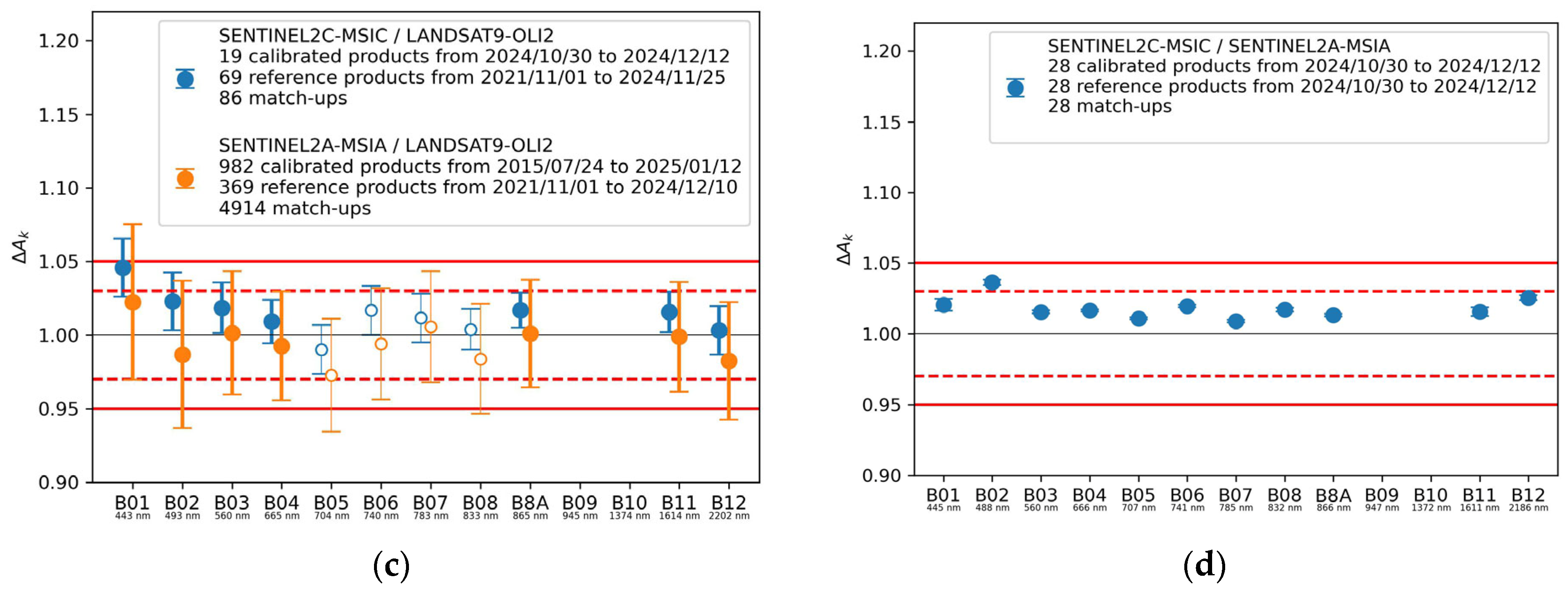
The SADE/MUSCLE cross-calibration results over desert sites are provided in Figure 16 for several reference missions: (a) MERIS, (b) Sentinel-3 OLCI-B and (c) LANDSAT-9. The good radiometric alignment of these missions is of primary interest for users, who may want to combine data in their studies. In every case, the results obtained for Sentinel-2C are provided in blue and the results from Sentinel-2A are shown in orange. These comparisons show that Sentinel-2A is in good agreement with the reference sensors whereas Sentinel-2C is a bit brighter.
The PICS method is a very efficient method to cross-compare different instruments and, thus, to get a precise bias estimation. A direct comparison of Sentinel-2C and Sentinel-2A is computed by limiting the dataset to the tandem phase. Over this period, the quasi-simultaneous acquisition reduces the uncertainties related to the atmosphere variations. In addition, the analysis relies on large PICS sites (100 km × 100 km) so that the uncertainty related to spectral response variations along the swath is reduced (cf. discussion in Section 5.1.2). The results are shown in panel (d) of Figure 16.
The same exercise is repeated over dome sites and the results given in Figure 17 confirm that Sentinel-2C is not well aligned with the reference sensors. Compared to desert results, the dispersion of Dome results is lower for the short wavelengths. The high altitude and the very dry atmosphere of the dome sites explain the improved efficiency of the atmospheric correction. The SWIR range can only be analyzed on the strict tandem acquisitions; for a larger temporal discrepancy, the snow microstructure is not stable anymore. In addition, these results are slightly less reliable than desert ones because the Sentinel-2 C dataset used was not accurately cloud-screened. The snow cover makes the cloud detection more difficult. The results are still very close to the desert ones, except for B02 which is a bit lower for dome results than for desert results. For both methods, B02 appears a bit brighter than the other VNIR channels; however, this behavior is more significant over desert sites. B02 has a large bandwidth compared to the other visible bands, which makes this spectral band more sensitive to interpolation errors. The difference in the spectral signature of desert and dome sites around 493 nm explains that B02 results vary a bit between these two PICS methods.

3.2.2. Absolute Calibration on Ocean Sites

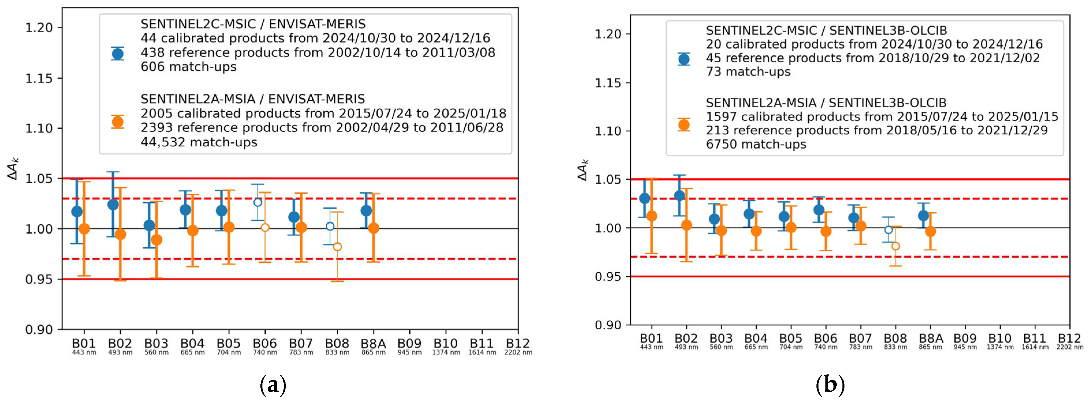
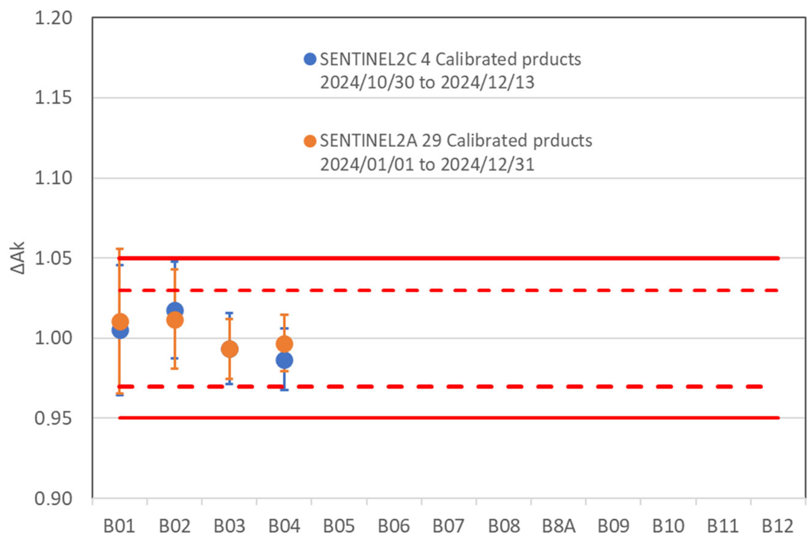
During the Sentinel-2C in-orbit commissioning period (i.e., September to December 2024) only four products have met the Rayleigh method conditions implemented in DIMITRI. More than 29 products from Sentinel-2A during 2024 have met the Rayleigh method conditions. The averaged ratios (TOA_obs/TOA_sim) and standard deviations computed by DIMITRI over the available products are presented in Figure 18. However, it is difficult to draw a solid conclusion from this result due to the limited number of acquisitions of MSI-C.
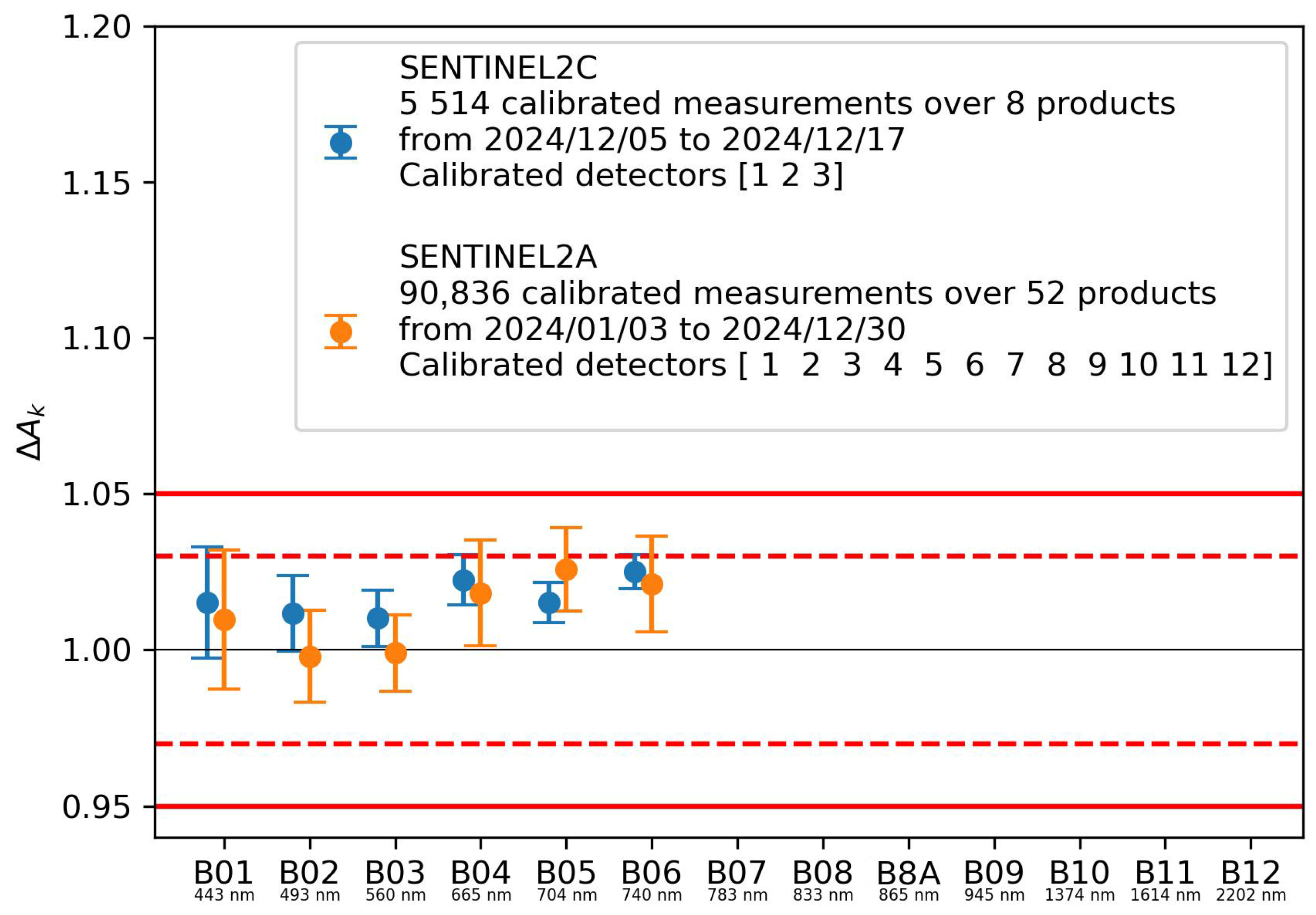
All results obtained with SADE/MUSCLE on ocean data are summarized in Figure 19. The Sentinel-2C results, in blue, include fewer measurements than the Sentinel-2A results, in orange, because they are limited by the three-month commissioning phase. In particular, the geometrical configurations over the ocean sites during this period were only suitable for detectors 1 to 3, with the other ones being more affected by clouds and Sun glint. Both sensors show a good consistency within 3% compared to the theoretical Rayleigh scattering. Unlike the PICS results, which clearly indicate a bias between Sentinel-2A and C, the results obtained over the ocean sites are less significant. This method is not the best one to establish a cross-calibration, especially due to the spectral response variability along the swath as discussed in Section 5.1.2.

3.2.3. Cross-Comparison and Inter-Band Calibration on DCC

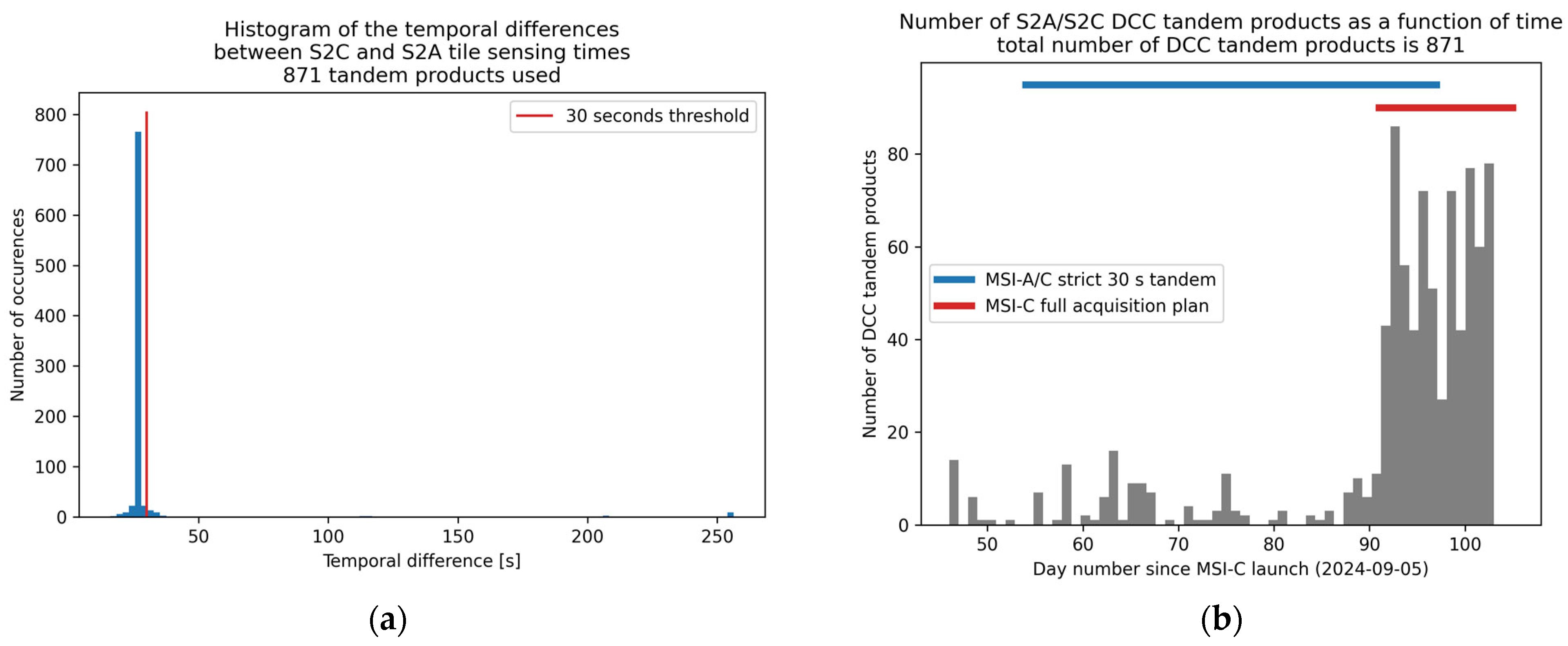
To get the most reliable cross-comparison results between Sentinel-2A and Sentinel-2C, the OPT-MPC method is focused on the tandem phase. Figure 20a presents the temporal differences between the MSI-A and MSI-C acquisitions; one can observe that more than 80% of the pairs of MSI-A and MSI-C products have been acquired with less than thirty seconds of difference. Some outliers remain, but they have not been filtered out as the method presented here is a statistical method and thus mainly relies on the number of products analyzed. These outliers are explained by the acquisition date of the products given in Figure 20b. One can observe that the MSI-A/MSI-C products are also used before and after the strict 30 s tandem period, during which the two satellites were observing scenes with less than 30 s of temporal difference. However, this is not a problem as satellites were also flying in a close configuration during these periods, albeit not as close as 30 s.
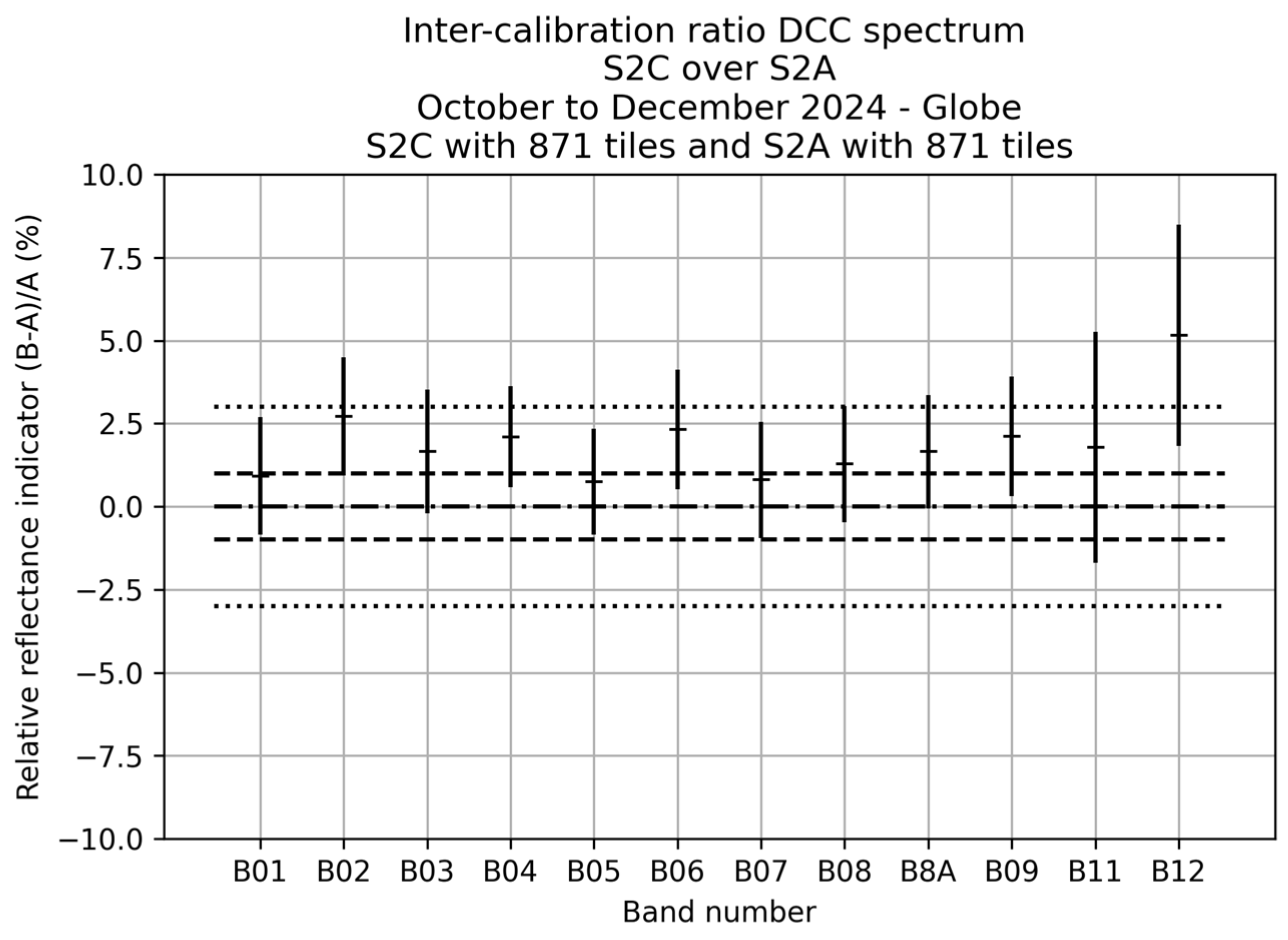
The relative difference between the radiometry of MSI-C and MSI-A is computed for each band using the OPT-MPC methodology presented in Section 2.2.4 and in Figure 21.
For the inter-band calibration results computed with SADE/MUSCLE, each spectral measurement of the satellite is compared to a simulation as described in Section 2.2.4. Therefore, the most important point is to filter the measurement conditions for which the simulation will be as accurate as possible. The temporal shift between the acquisition is less significant in this case than for the cross-comparison case described hereinabove (i.e., the OPT-MPC method). The processed measurements are not necessarily taken during the tandem phase; priority was placed on collecting enough measurements, covering the entire swath.
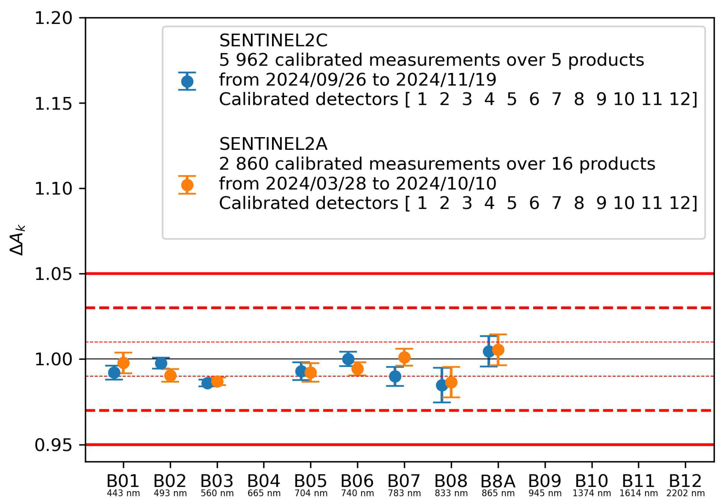
Figure 22 shows the SADE/MUSCLE inter-band calibration results both for Sentinel-2C in blue and Sentinel-2A in orange. Both satellites have a spectral consistency below 1% for most bands and 1.5% in the worst cases. As expected, the result dispersion increases with wavelength because the DCC model is less accurate for large wavelengths. In particular, the largest discrepancy between Sentinel-2A and Sentinel-2C is obtained for B07 (783 nm) and the largest inter-band misalignment is obtained for B08 (833 nm). These worst cases at longer wavelengths may be linked to the method. Further investigations on a larger Sentinel-2C dataset will be required to distinguish between an instrument-related effect or a method artifact, and to better understand the deviation observed for B03 (560 nm).

3.2.4. Absolute Calibration over the Moon

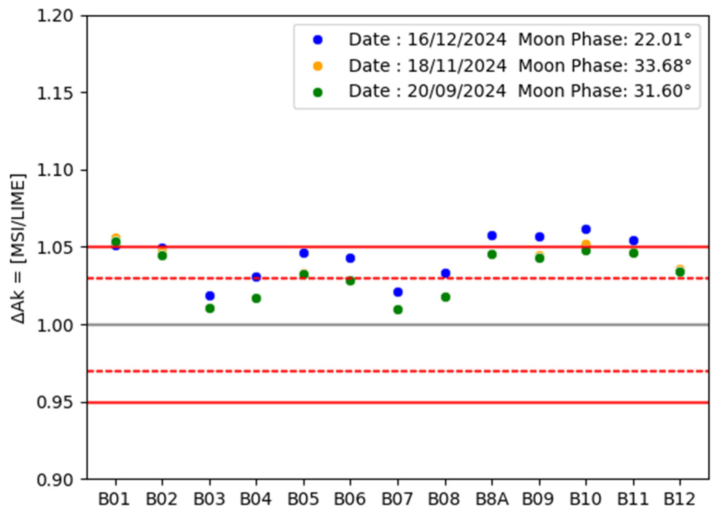
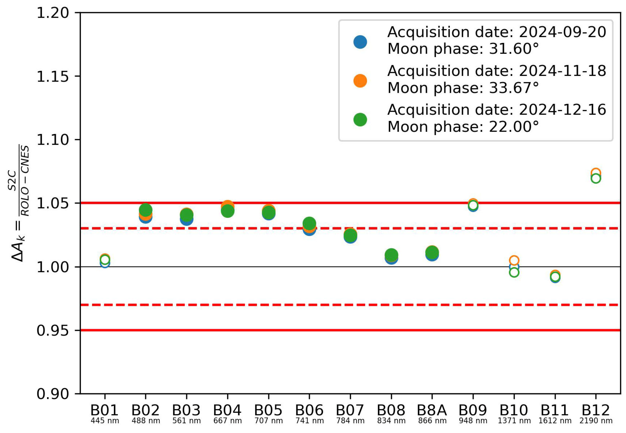
Figure 23 shows the results of the comparison between the Sentinel-2C MSI lunar irradiances and the calibration model LIME as described in Section 2.2.5. The irradiances have been derived from their respective instrument L1B datasets. Differences observed in the results can thus originate from both the irradiance calculation and the output of the LIME model.
In general, the overall radiance level of the instrument seems to be slightly brighter than the LIME model for these acquisitions. When taking the average over the three acquisitions, all bands remain within the expected requirement of 5%, except for B01. Note that the central wavelength of this band is at the edge of the model spectral range where the results tend to be slightly more uncertain.
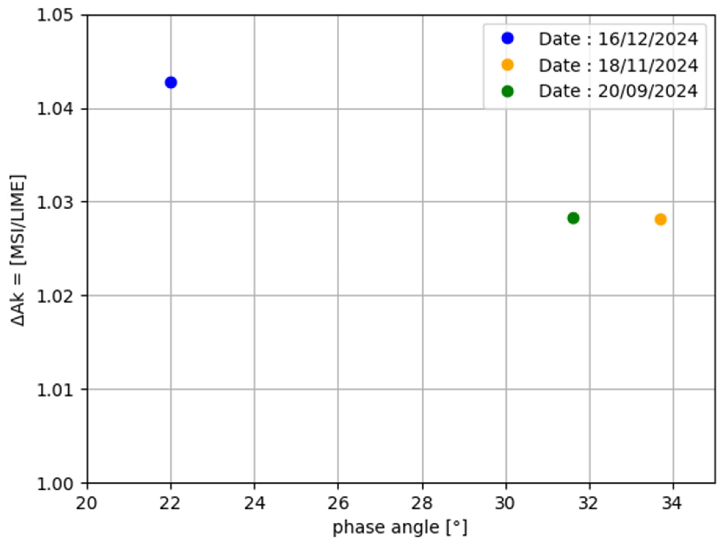
The acquisition of the Moon at a lower phase angle (performed on 16 December 2024) generally has a higher band gain compared to the other two acquisitions. The cause is currently unknown, as it could originate from both image processing and model output. The dependency on phase angle is displayed in Figure 24.
The difference between the acquisitions is less than 2%, the currently expected uncertainty level of the LIME model. The spectral shape in the results remains within the levels observed from the other validation methods.
The comparison between Sentinel-2C Moon acquisitions and the ROLO-CNES model explained in Section 2.2.5 is provided in Figure 25. Over the entire spectral range, the monthly calibration results are very close to each other despite differences in the Moon phases: this shows that the satellite radiometry is stable and that the model takes into account the Moon phases accurately. On the SWIR range, even if all monthly results are very well aligned, some radiometric bias may exist due to the ROLO-CNES model extrapolation, in particular the large discrepancy between B11 and B12, which is not confirmed by PICS results (cf. Section 3.2.1). On the contrary, the VNIR results are compatible with the other methods: Sentinel-2C is brighter than expected. The spectral bell shape of the calibration results is not understood yet; it may be related to an increased inaccuracy near the boundaries of the model validity domain. The DCC inter-band calibration results of Figure 22 do not confirm this spectral signature; therefore, further investigations of the Moon method will be required.

3.2.5. Cross-Comparison Using Global Earth Tandem

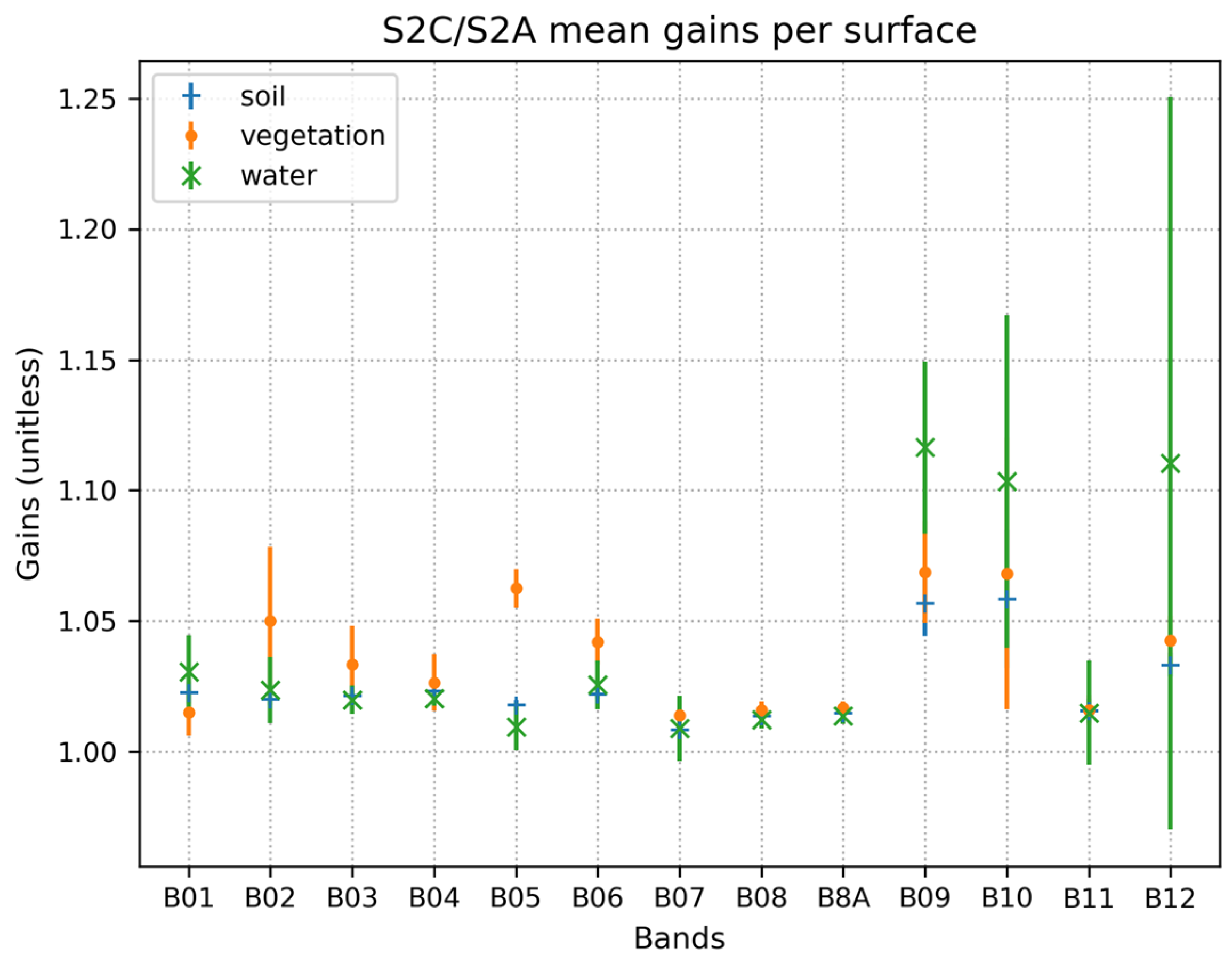
As explained in Section 2.2.6, S2C/S2A gains for tandem acquisitions are computed for different classes of pixels: bare soil, vegetation, and water. The results are presented in Figure 26 below, reporting for each pixel class the average value across the field of view and the dispersion among detector modules.
For bands B01, B03, B07, B8A and B11, the results are remarkably consistent across the different surfaces and show relatively low dispersion between detector modules. For bands B02, B03, B05 and B06, the results for the vegetation class are significantly above those for the other surfaces. The discussion presented in Section 5.1.1 shows that most of the differences can be attributed to the difference in spectral response functions between the two sensor units, although the difference for band B02 is higher than expected.
For the atmospheric bands B09, B10 and B12, the results over water pixels are significantly higher than those for other classes. Here again the impact of differences in spectral responses is a likely explanation. For B11, the two sensors have more similar response functions, and this band is not affected by water vapor absorption. The effects observed in Figure 26 are larger than those shown by the simulations in Section 5.1.1. However, these simulations consider only a medium water vapor concentration. Another important contributor for the SWIR bands is the Sun-glint signal, which induces a systematic difference due to the small time lag between S2A and S2C. Sun-glint effects also explain the large variations among detector modules: it can be verified that higher gain ratios are observed on the easternmost detector, which is the one most affected by Sun-glint.
In conclusion, the gain coefficients estimated over bare soil pixels are considered more reliable because they are less impacted by differences in spectral responses and Sun-glint effects.
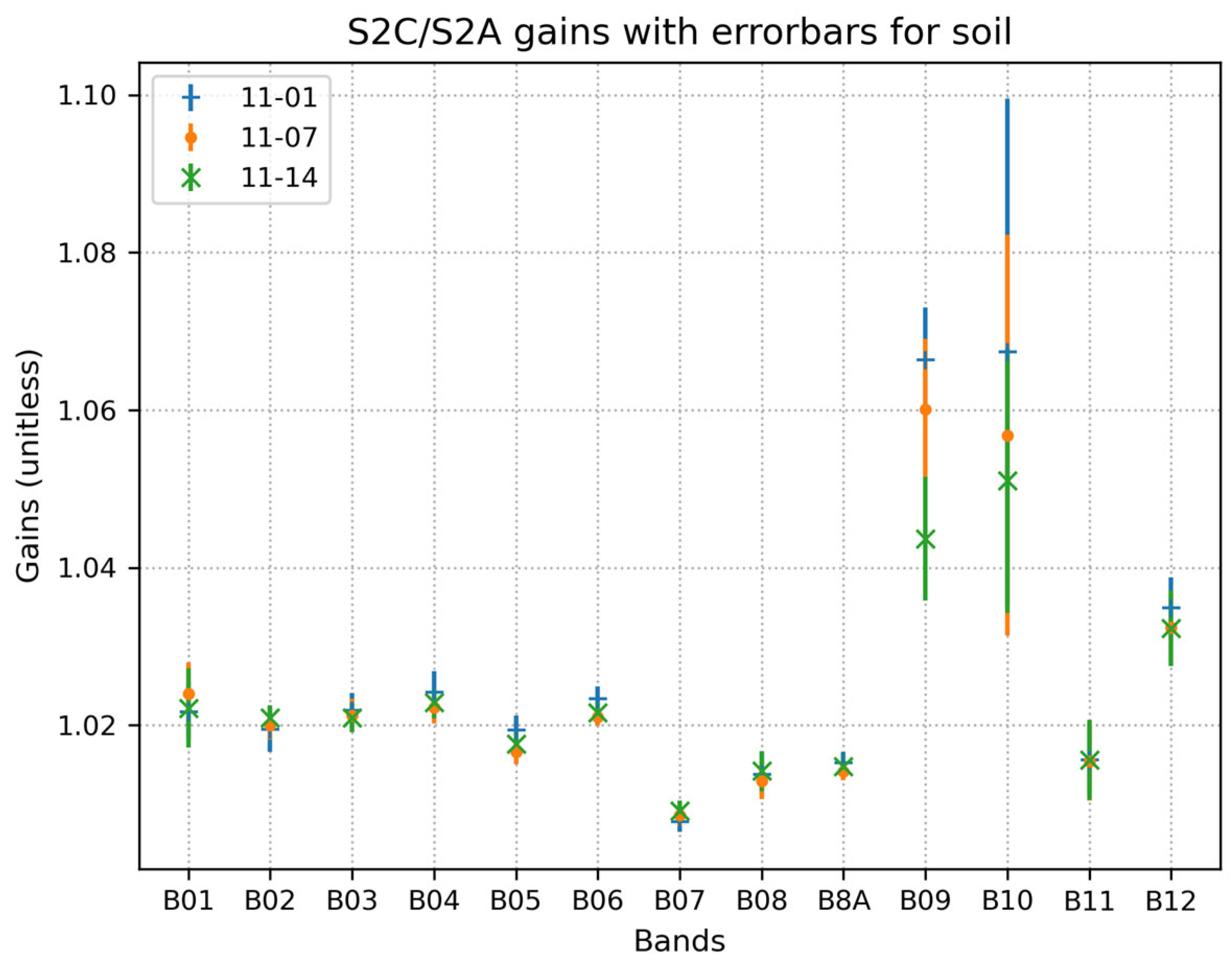
In order to assess the stability of the estimated gains over time, we performed the same analysis over three consecutive 6-day periods. The results presented in Figure 27 below present a remarkable stability except for the atmospheric bands B09 and B10. The latter is most likely due again to the differences in the spectral response function and the sensitivity to water vapor concentration for these bands. Indeed, the average water vapor concentration can be significantly different between the three periods. As a result, the direct tandem comparison method may not be applicable to these bands.

4. Sentinel-2A/Sentinel-2C Radiometric Harmonization

The objective for the commissioning phase regarding the radiometric calibration was to keep any relative error among Sentinel-2 units below 3% (threshold) and ideally below 1% (goal). As a reminder, during the collection 1 reprocessing, a 1.1% discrepancy between Sentinel-2A and B was corrected [55], resulting in a coherent dataset between the first two units. Achieving this objective for Sentinel-2C within a period of 3 months was a specific challenge as most vicarious inter-comparison methods require long periods to provide consistent results. Thanks to the Sentinel-2A/Sentinel-2C tandem, efficient radiometric cross-calibration became possible.

4.1. Synthesis of Results and Best Estimate of Relative Gains

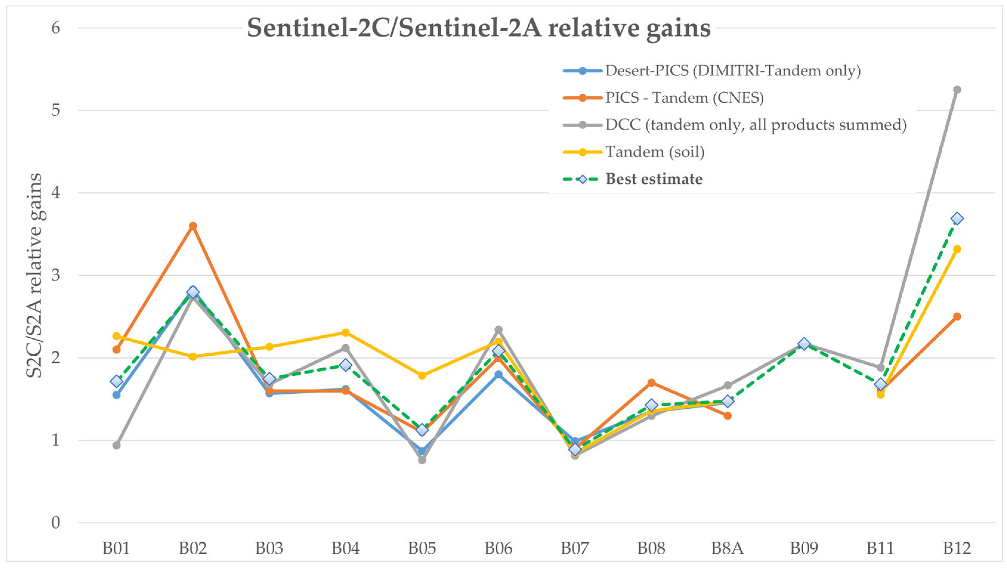
The following figure (Figure 28) reports the results obtained by the different methods described in the previous sections. Numerical values are provided in Table 4.
The results of all of the different methods are remarkably convergent. We find a slightly higher spread for bands B01, B02, B05 and B12, which may be explained in part by the impact of the differences in spectral responses for these bands. We consider that the best estimate can be computed by averaging the four methods for each band.
For the water vapor band B09, results are not available for the PICS method. For the tandem method, a robust estimate could not be provided either because of the difference in sensitivity to water vapor between Sentinel-2A and Sentinel-2C. Therefore, our best estimate is provided by the DCC method only. Note that CNES’s Moon calibration results (based on extrapolation of the ROLO model) indicate a higher absolute bias (above 5%).
The situation for the cirrus band B10 is even less favorable. The PICS method is not applicable, and the results of the DCC method are impacted by saturation. As far as tandem inter-comparisons are concerned, there is a considerable dispersion in the results (between detectors, between surfaces and between time periods): no robust estimate can be provided. It is likely that the results are affected by other effects (dark level stability for instance) than a simple calibration gain difference. At the present time, no best estimate can be provided for this band. CNES’s Moon calibration results indicate a nearly zero absolute bias for this band.

4.2. Implementation

To improve the inter-calibration between Sentinel-2A and Sentinel-2C, it was decided to apply a vicarious adjustment to the radiometry of Sentinel-2C. First, a uniform correction factor was applied to all the bands except B10 and B12. While the relative spectral profiles of Sentinel-2A and S2C show some differences, our analysis does not allow us to determine which satellite has the most accurate relative radiometry. Therefore, we prefer to keep the spectral profile of Sentinel-2C unchanged. For B10, no correction has been applied since there was not sufficient evidence that a positive bias existed for this band. Regarding B12, a specific correction was applied since the best estimate indicated a significantly higher bias for this particular band.
Taking advantage of the operational deployment of Sentinel-2C, a minor improvement of the calibration method (correction of the diffuser incidence angle) has been implemented. This led to a small shift in the radiometry of Sentinel-2A and Sentinel-2B (+0.11% and −0.11% respectively).

4.3. Validation of the Results

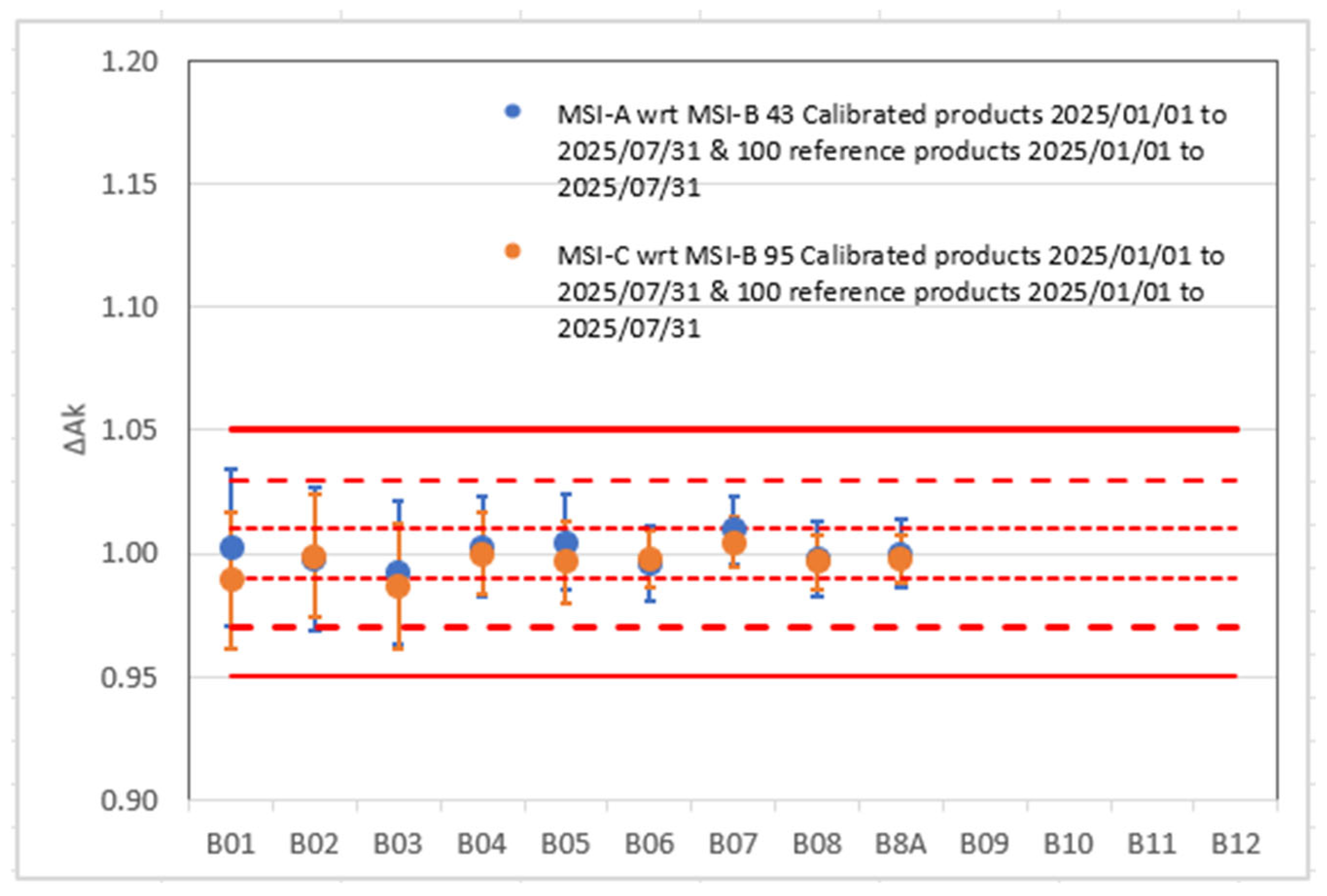
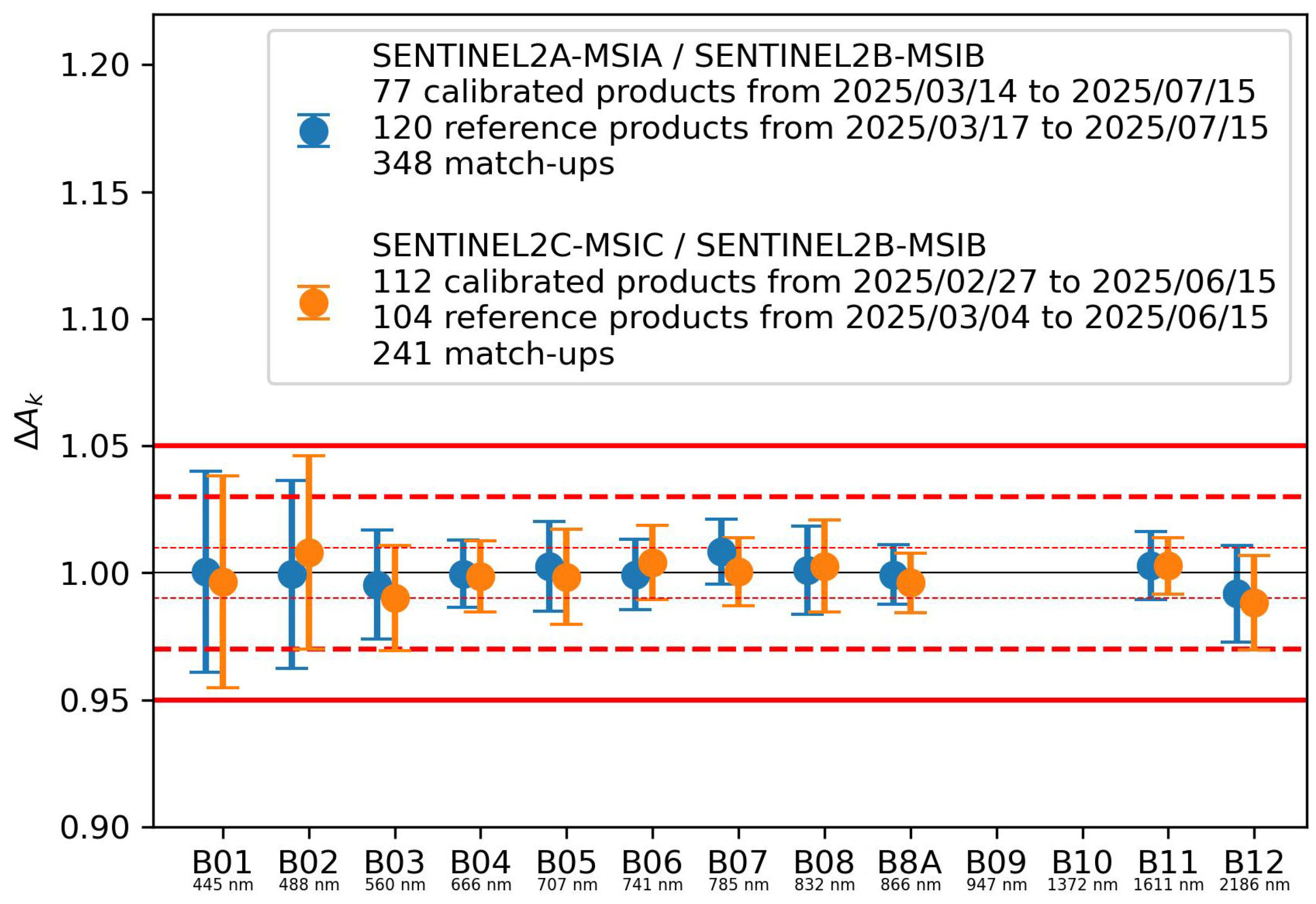
While writing this paper, the Sentinel-2C operational phase has begun and some initial cross-calibration results have become available. The radiometric alignment of the Sentinel-2 constellation analyzed by DIMITRI and SADE/MUSCLE is provided in Figure 29 and Figure 30 respectively. Even if the available dataset is still limited to recent products, these initial results show that the Sentinel-2C correction is well implemented and brings the entire Sentinel-2 constellation within 1% or better.
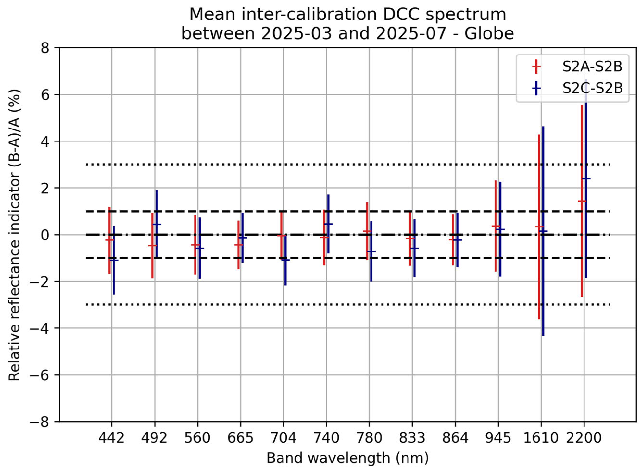
Similarly, the radiometric alignment of the Sentinel-2 constellation was analyzed between March and July 2025 using Deep Convective Clouds after harmonization of the sensors. The results are provided in Figure 31. Contrary to the results shown in Section 3.2.3, the products used here are not limited to those acquired simultaneously by the two satellites, as the tandem phase is over. All the products available for each satellite are used, with at least 1000 per month for Sentinel-2B and Sentinel-2C and at least 250 for Sentinel-2A (limited number due to a limited acquisition plan). One can observe that for all of the analyzed bands, relative differences using Sentinel-2B as a reference are lower than 1.5%, except for band B12 where the relative difference is around 2%.
Following radiometric harmonization, the cross-calibration results obtained on PICSs by both DIMITRI and SADE/MUSCLE, as well as those computed by the OPT-MPC on DCC, demonstrate that the radiometric consistency among the Sentinel-2 instruments (A, B and C) is better than 1.5%. The only exception is B12 when using the DCC method. This discrepancy was anticipated, as the harmonization coefficient provided for this band differed from the others (cf. Section 4.1).

5. Discussion

As already mentioned, one of the most demanding tasks performed during the commissioning phase was the radiometric alignment of the sensors. We take this opportunity in this section to discuss the main sources of uncertainty that may affect this bias estimation.

5.1. Spectral Response Differences

5.1.1. Variations Between Satellite Units

The radiometric bias between Sentinel-2A and Sentinel-2C is characterized on tandem data. Most uncertainty sources affecting vicarious methods disappear in this context, namely: radiative transfer and atmospheric modeling errors, surface BRDF modeling errors, polarization sensitivity and reference scene temporal variability. One of the remaining sources of error concerns differences in spectral responses, as described in Section 1.2. The correction of these differences requires a knowledge of the spectral profile of the scene.
For the Pseudo-Invariant Calibration Site (PICS) method, the spectral profile of the desert scene is estimated by a combination of a reference sensor and on-ground measurements. For the DCC method, the spectral profile of the clouds is estimated using a reference sensor. For the direct pixel comparison, the impact is limited by selecting surfaces with a smooth spectral profile.
The measurement variations induced by the spectral response variation can be estimated by a fine radiative transfer code modeling the different radiative effects contributing to the TOA signal (mainly atmospheric scattering by molecules and aerosols and gas absorption). The SOS-ABS radiative transfer code has been selected for these simulations [40].
The conditions of simulations correspond to typical situations:
  • The solar zenith angle is 40°;
  • The atmospheric pressure is 1013 mbar;
  • The aerosols are of the continental type (WMO model) for an optical thickness AOT550 = 0.5 at 550 nm;
  • The amount of ozone is 350 Dobson;
  • The amount of carbon dioxide is 410 ppmv;
  • The amount of methane is 1.9 ppmv;
  • The water vapor amount is high to enhance absorption effects: 4.5 g/cm2;
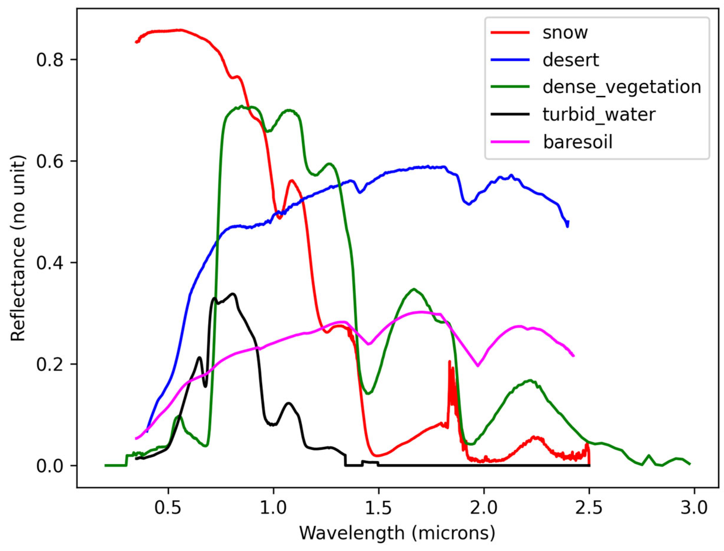
  • Five types of surfaces: dense vegetation, snow, turbid water, desert and bare soil (from USGS Spectral Library Version 7). Their spectra are shown in Figure 32. Note that the turbid water is bright from 0.5 to 1 µm and dark in the SWIR range.
Outputs are delivered for a viewing zenith angle of 10° in the solar principal plane. The gaseous absorption is modeled with a spectral resolution of 10 cm−1 for the VNIR bands and 5 cm−1 for the SWIR bands to properly cover the shape of the spectral bands and mitigate the computation time. Radiative transfer calculations are performed using a consistent spectral step (of 10 or 5 cm−1). A convolution with the different instrument spectral response functions (ISRFs) is finally applied to obtain the TOA reflectance observable by the sensors.
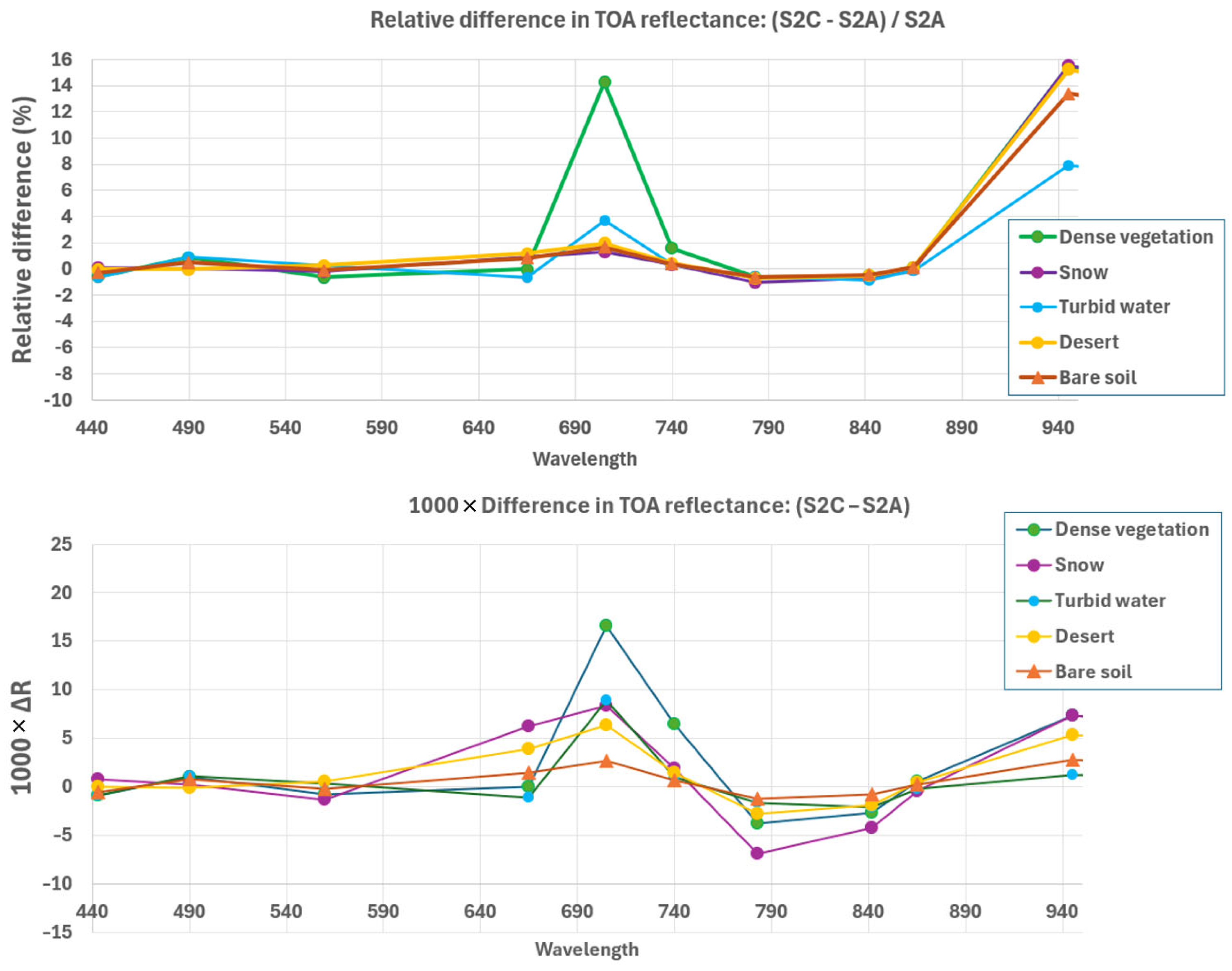
Figure 33 and Figure 34 show, respectively for the VNIR and SWIR bands, the absolute and relative difference between Sentinel-2C and Sentinel-2A TOA reflectance simulated for the different surface types.
What is clearly noticeable is that certain bands may have very different values of reflectance observed between MSI-C and MSI-A while they are considered to deliver the same measurements. For a relative comparison, this is mainly the case for the B05 band (705 nm) over vegetation and the B09 band (945 nm) and the B12 band (2190 nm) over snow. We can see that the observations over desert and bare soil are less dependent on the difference in spectral band definition and thus are the most appropriate for the tandem comparison. Note that the relative results for the B10 band are not relevant as the water vapor absorption is strong and leads to very small TOA reflectance.
Finally, Table 5 gives another view of the results with quantitative values of the difference in simulated reflectance between MSI-C and MSI-A.

5.1.2. In-Swath Variations

The spectral responses taken for Sentinel-2A and Sentinel-2C in the previous discussion only consider an averaged spectral response of the whole instrument. Every tool described in Section 2 assumes an averaged spectral response. However, within a given instrument, the spectral responses may vary slightly from one pixel to another and from one detector to another. For Sentinel-2C, the on-ground characterization has given access, for the first time on a Sentinel-2 instrument, to a spectral response per pixel for the entire swath.
Table 6 gives the extremum values, average values and standard deviation, per band, for the central wavelength and full width at half maximum (FWHM). The range of variation in the central wavelength over the swath is between 0.6 and 4.3 nm, depending on the considered band. The FWHM varies by 0.6 to 4.6 nm, except for the B08 band for which the FWHM variation over the pixels reaches 34.1 nm (note that this band is a broad band). The B08 band is also the VNIR band with the highest variation in its central wavelength over the swath.
Based on these characterizations, the sensitivity of the SADE/MUSCLE results to the spectral response is evaluated. To do so, typical TOA spectra from each vicarious calibration target are simulated and convolved with the per-pixel spectral response on one side and with the averaged spectral response on the other side. Then, the per-pixel simulations are averaged together as in the vicarious calibration methods, i.e., over a 960 m × 960 m area for DCC and oceans, a 20 km × 20 km area for deserts and a 100 km × 100 km area for domes. All possible positions of the vicarious target are tested across the swath and, for each case, the discrepancy between the simulations obtained by considering the per-pixel spectral response or the global spectral response is computed. For the sake of readability, only the results obtained for band B03 (561 nm) are given in Figure 35.
For the vicarious targets, the per-pixel spectral response variability can induce more than 0.5% variation in the measurements in the worst case. As expected, when the vicarious calibration method is based on large areas—such as the PICS ones—the results are less sensitive to the position within the swath. Since the sensitivity is mainly linked to the calibration site size, the results computed by DIMITRI are affected by an equivalent variability. To mitigate the induced uncertainty, the SADE/MUSCLE best bias estimate between Sentinel-2A and Sentinel-2C provided in Section 4.1 is specifically computed on large desert sites instead of the small sites. In this case, the per-pixel spectral variation is below 0.1% for all bands (except B01 and B12, which are higher at 0.5% and 0.3%, respectively).
The vicarious methods based on small areas such as ocean and DCC are more sensitive to this uncertainty. In particular, it explains why the bias between Sentinel-2A and Sentinel-2C cannot be estimated on ocean sites. When the Sentinel-2C dataset can cover a larger period, these methods could be used to experimentally evaluate the per-pixel spectral sensitivity variation and compare it to the on-ground characterization. In addition, the vicarious calibration tools may be adapted to take into account this variability.

5.1.3. Conclusions

In conclusion, the spectral variations between Sentinel-2A and Sentinel-2C can induce a variation in the measured reflectance by several percents even for the exact same target. This effect is not due to a bad cross-calibration of the two instruments; they simply do not measure the exact same spectral range. The end-user applications relying on time series including Sentinel-2A, B and C units have to take into account the per-instrument spectral response to avoid any issues. In addition, the spectral sensitivity variation per pixel of the swath can induce around half a percent of variation in the measurements, with a maximum of 4.5% for B05 and 2.6% for B06 over grass. This residual error cannot be easily included in end-user applications and is part of the uncertainties budget. The error levels provided here are approximated since they heavily depend on the input spectrum.
As far as our results are concerned, the impact of inter-unit differences are accounted for:
  • The PICS, ocean, Moon and CNES DCC methods rely on hyperspectral models which are convolved by the average sensor SRF.
  • For the OPT-MPC DCC method a transfer hyperspectral sensor (EnMAP) is used to compute SBAF between the two sensors.
  • The global tandem cross-comparison on the other hand does not apply any spectral adjustment. The impact can however be analyzed by comparing results obtained on different surfaces (soil, vegetation, water) with simulation results. From this analysis we expect results over bare soil to be less affected by SRF differences.
The impact of in-swath variations on the results has also been analyzed in the previous section for several methods. The impact was shown to be limited except for the ocean method.

5.2. Mission Dynamic Range

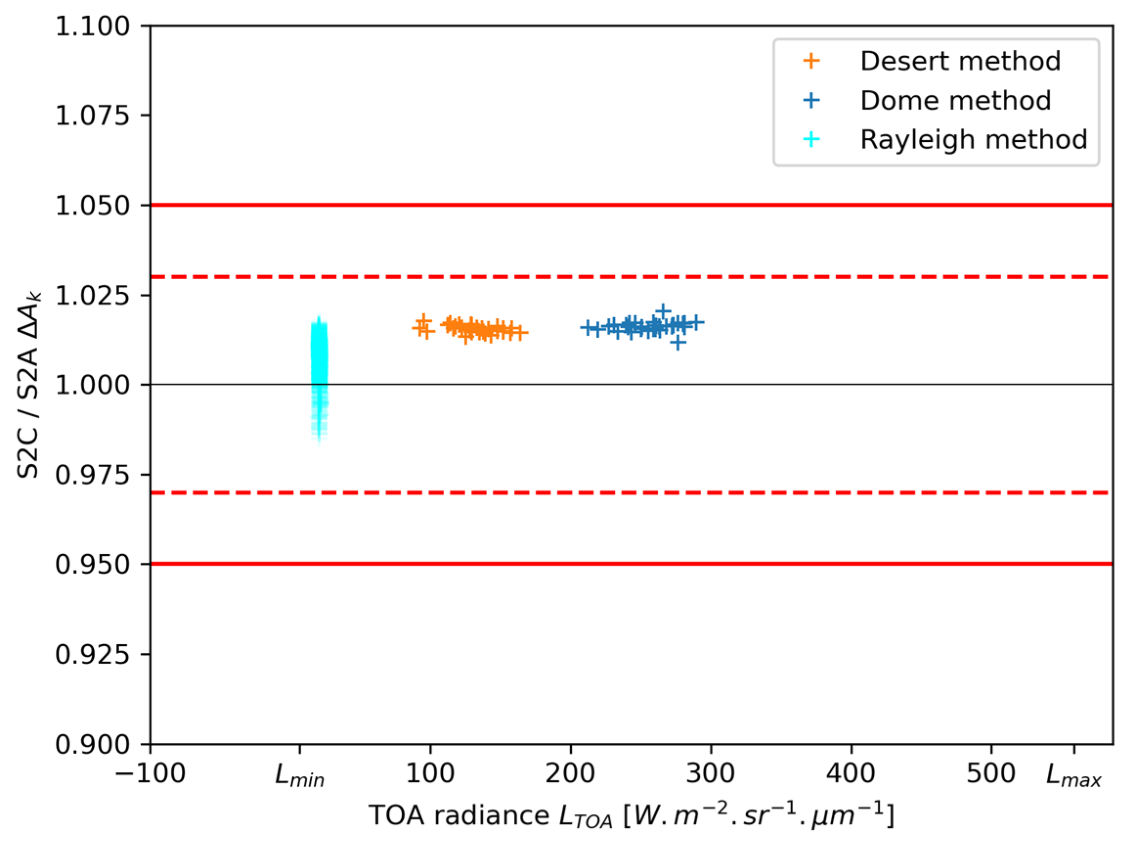
The combination of all methods described in Section 2.2 enables us to cover the mission dynamic range as much as possible. In particular, the bias between Sentinel-2A and Sentinel-2C should be analyzed for various input levels in order to detect any non-linear effects that may appear. As an example, in Figure 36, all the SADE/MUSCLE results are plotted together with their associated target input radiance for band B03 (561 nm). This analysis confirms that whatever the input radiance, the bias seems to be the same. Note that the satellite cross-comparison over ocean gives highly dispersed results due to the spectral response sensitivity—as explained in Section 5.1.2—and cannot be used reliably.

5.3. Temporal Stability

The bias measured between Sentinel-2A and Sentinel-2C was significant enough to disturb downstream applications; therefore, it was of primary interest to correct it as soon as Sentinel-2C became operational. The bias could only be estimated over a 3-month period, which is relatively short and may not take into account potential seasonal or long-term variations. More precisely:
  • Seasonal effects affecting the validation method may bias the results obtained over a short period of time. This aspect is investigated later in this section in the case of the PICS method and the tandem method.
  • Seasonal effects may also affect the Sun diffuser calibration method. Based on the experience acquired with Sentinel-2A and B, we expect such effects to be very limited. In addition, the optimized in-flight Sun diffuser BRDF described in Section 2.1 should reduce them even further.
  • Long-term drift (linked, e.g., to diffuser aging) may also affect the Sun diffuser calibration. Based again on experience from Sentinel-2A and B, we expect such drift to be very small as all vicarious methods indicate a very stable radiometry for both units. Nevertheless, the radiometric stability of Sentinel-2C shall be continuously monitored in the future.
In order to obtain an estimation of the uncertainty induced by the short calibration period, the Sentinel-2A dataset is analyzed.
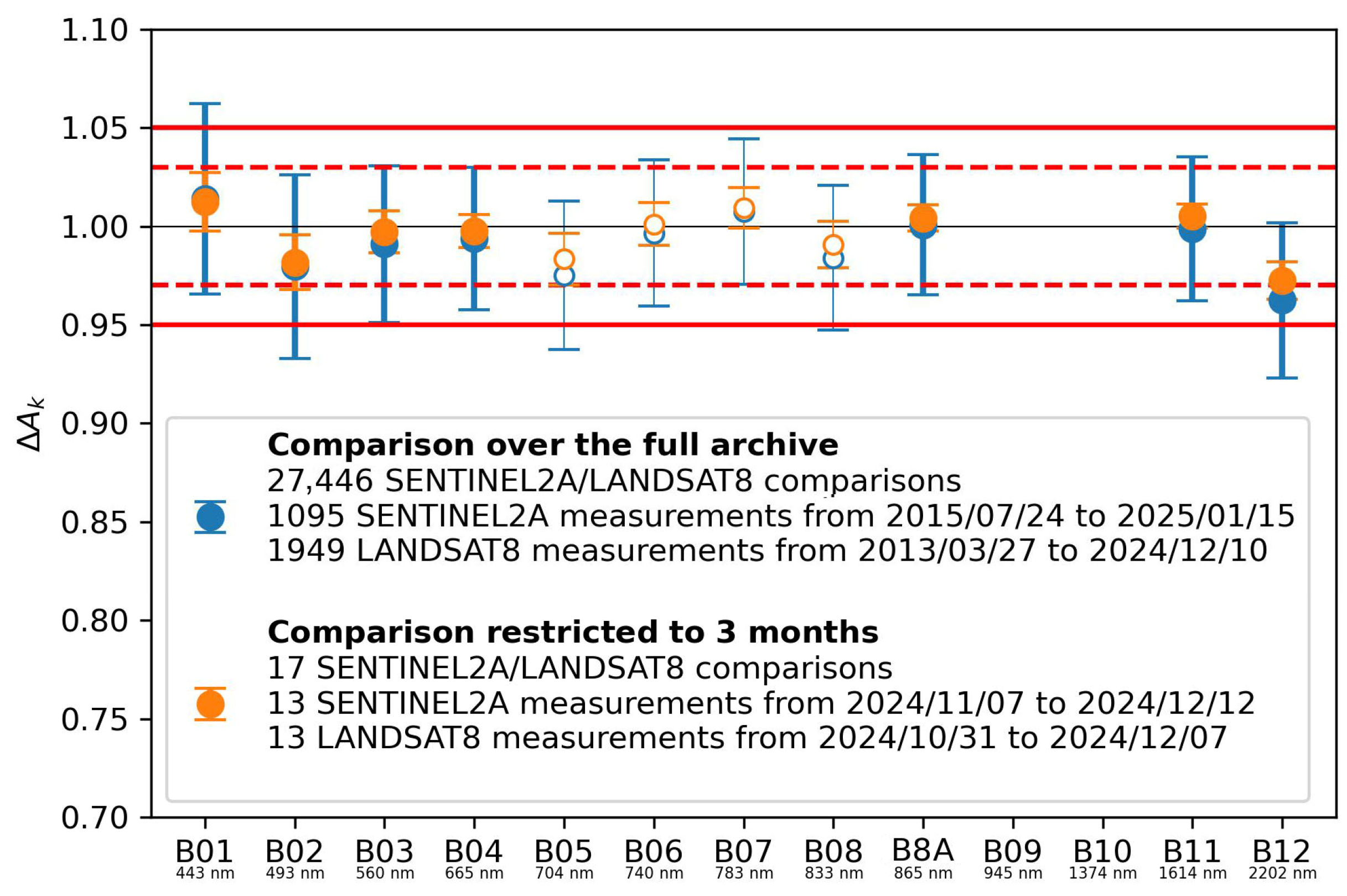
In Figure 37, the cross-calibration over PICSs between Sentinel-2A and LANDSAT-8 is provided. In blue, the calibration includes all available data whereas in orange, the dataset is restricted to 3 months, as in the commissioning phase. This comparison gives the discrepancy induced by the temporal restriction of the calibration results. This discrepancy should be a reasonable estimation of the uncertainty affecting the bias computed between Sentinel-2A and Sentinel-2C. It appears that it depends on the spectral bands, with a variation between 0.2% (on short wavelengths) and 1% (especially on the SWIR) with a 0.5% average. So, the uncertainty which may affect the bias estimation is rather low compared to its value (around 2%): the immediate correction is thus relevant. After a one-year operational period of Sentinel-2C, an additional correction could be applied if seasonal variations are detected.
For the tandem global inter-comparison, the number of measurements is large despite the short duration of the tandem phase. It was therefore possible to monitor the evolution of the results over three periods of time, as shown in Figure 27 (Section 3.2.5). The relative gains estimated for those three periods are consistent within ±0.25%, except for the atmospheric bands B09 and B10 which are strongly affected by water vapor. There is no indication of a statistically significant trend over this period. We can therefore expect that the results are not strongly affected by seasonal bias.

6. Conclusions and Lessons Learned

The calibration and validation activities performed during the commissioning phase of Sentinel-2C ensured that the images are of equivalent or better radiometric quality than those of Sentinel-2A in terms of Signal to Noise Ratio, Fixed Pattern Noise, and Modulation Transfer Function. However, there was converging evidence of an inter-sensor radiometric bias, which led to the introduction of a vicarious alignment to improve the operability of the sensors. The determination of this vicarious alignment depended crucially on:
  • The use of quasi-simultaneous acquisitions thanks to tandem operations;
  • A fine assessment of the impact of differences in spectral responses for different types of scenes;
  • The use of several radiometric validation approaches to ensure a robust estimation of inter-calibration gains for all spectral bands.
This activity was performed within the temporal constraint of the commissioning phase and enabled the implementation of the correction from the start of nominal operations in January 2025.
Some lessons learned and recommendations could be noted for the future.
First, it proved very useful that two different teams using different software processed the same calibration data (Sun diffuser and dark acquisitions). This allowed the detection of minor configuration errors that might otherwise have gone unnoticed. The validation exercise was also handled by two different teams with different methods, a synergy which was key to derive a reliable correction of the S2C radiometry. We recommend continuing this effort for future commissioning phases. This includes processing calibration data with two different software tools and assessing performances with at least two different methods.
Second, data acquired during the tandem held their promise by ensuring a very robust and stable assessment of inter-calibration gains for all vicarious methods. For Sentinel-2B, it had been necessary to wait for one year of operation to obtain robust estimates of the inter-satellite gains and implement a radiometric adjustment. Thanks to the Sentinel-2C tandem, the estimates were obtained at the end of the commissioning phase, and the adjustment was implemented from the start of nominal operations, minimizing the impact for downstream users. Although this has not been discussed in the present paper, data acquired during the tandem phase also proved valuable to assess measurement uncertainty using the Sentinel-2 Radiometric Uncertainty Tool [56,57]. We believe that this dataset could also be relevant to assess the uncertainty of downstream products. In addition, an analysis of the Sentinel-2A/Sentinel-2C co-registration allowed us to assess the impact of focal plane geometric calibration errors and high-frequency platform oscillations. While the tandem phase required some maneuvers which increased the commissioning phase timeline, the net result was positive since it allowed much faster geometric and radiometric performance characterization. For these reasons, we recommend the implementation of short tandem phases for constellation missions whenever possible. A period of one month was considered sufficient, provided that enough data is acquired.
However, we still encountered some limitations in our ability to accurately inter-calibrate the sensors. Atmospheric absorption bands (B09 and B10) are subject to many instrument effects such as differences in spectral responses, stray light, and non-linearities. We noted that obtaining robust inter-calibration gains for these bands is very difficult. On the other hand, the impact on product data quality is much less critical than for surface reflectance bands. More surprisingly, we also found some issues in assessing the inter-sensor bias for band B12 which is only slightly affected by water vapor. There was significant dispersion among the different methods which requires further investigation.
The sensitivity analysis on differences in spectral response function revealed that the impact on some spectral bands (B05 in particular) can be very high, and downstream users may not be able to correct for these differences in their application. For future missions, we recommend paying more attention to uniformity and inter-unit repeatability of the spectral filters for bands which are sensitive to spectral response differences.
Finally, the Moon images showed some potential as a solid reference for Sentinel-2 radiometric calibration. However, some further work is required in order to better understand the differences between the different models and to consolidate the radiometric assessment of the SWIR bands. The Moon images were also useful to investigate stray light effects; this point will be reported elsewhere. Moon acquisitions with other Sentinel-2 units are recommended.

Author Contributions

Conceptualization, S.C.; methodology, D.R., B.L., B.A., L.R., A.D., S.A. and S.C.; software, D.R., B.L., B.A., L.R., A.D., S.A. and E.H.; validation, D.R., B.L., B.A., L.R., A.D., S.A. and E.H.; formal analysis, D.R., B.L., B.A., L.R., A.D., S.A. and S.C.; writing—original draft preparation, S.C., D.R., B.L., B.A., L.R., A.D., S.A. and S.E.; writing—review and editing, all authors; supervision and funding, R.M., R.I. and V.B. All authors have read and agreed to the published version of the manuscript.

Funding

This research was funded by ESA and the European Union in the frame of the Copernicus Optical Mission Performance Cluster under contract 4000136252/21/I-BG and the CNES Routine Operational Phase Support contract (4000145478/24/I-AG).

Data Availability Statement

All original Sentinel-2 data used for this research is available upon request.

Acknowledgments

The authors acknowledge the support from the Optical Mission Performance Cluster operation team for collecting, preparing and processing Sentinel-2 data. The support and feedback from ESA/ESTEC’s Sentinel-2C Commissioning team and ESA/ESRIN Sentinel-2 team is gratefully acknowledged.

Conflicts of Interest

Authors S.C., B.A., A.D. and L.R. were employed by ACRI-ST. Authors B.L., S.E., E.H. and R.M. were employed by CS group. Author S.A. was employed by VITO. Author D.R. was employed by CNES. The remaining authors declare that the research was conducted in the absence of any commercial or financial relationships that could be construed as a potential conflict of interest.

Abbreviations

The following abbreviations are used in this manuscript:
BOABottom-of-atmosphere
BRDFBi-Directional Reflectance Distribution Function
CWLCentral wavelength
DCCDeep Convective Clouds
EOEarth Observation
FPNFixed Pattern Noise
FWHMFull width half-maximum
MTFModulation Transfer Function
PICSPseudo-Invariant Calibration Site
SNRSignal to Noise Ratio
SWIRShort-Wave Infra-Red
TOATop-of-atmosphere
UTCCoordinated Universal Time
VNIRVisible and near infra-red

References

  1. Gascon, F.; Bouzinac, C.; Thépaut, O.; Jung, M.; Francesconi, B.; Louis, J.; Lonjou, V.; Lafrance, B.; Massera, S.; Gaudel-Vacaresse, A.; et al. Copernicus Sentinel-2A Calibration and Products Validation Status. Remote Sens. 2017, 9, 584. [Google Scholar] [CrossRef]
  2. Pahlevan, N.; Sarkar, S.; Franz, B.A.; Balasubramanian, S.V.; He, J. Sentinel-2 MultiSpectral Instrument (MSI) Data Processing for Aquatic Science Applications: Demonstrations and Validations. Remote Sens. Environ. 2017, 201, 47–56. [Google Scholar] [CrossRef]
  3. Toulemont, A.; Fernandez, V.; Mavrocordatos, C.; Mandorlo, G.; Laberinti, P. Sentinel-2C Instrument New Features and First Instrument Performance Characterization. In Proceedings of the Sensors, Systems, and Next-Generation Satellites XXIII; SPIE: Bellingham, WA, USA, 2019; Volume 11151, pp. 95–100. [Google Scholar]
  4. Toulemont, A.; Olivier, M.; Clerc, S.; Bellouard, R.; Reina, F.; Gascon, F.; Luce, J.-F.; Mavrocordatos, C.; Boccia, V. Copernicus Sentinel-2C/D Multi Spectral Instrument Full Field of View Spectral Characterization. In Proceedings of the Sensors, Systems, and Next-Generation Satellites XXV; SPIE: Bellingham, WA, USA, 2021; Volume 11858, pp. 194–203. [Google Scholar]
  5. Krijger, M. Diffuser BRDF Analysis Modelling from On-Orbit Measurements; Earth Space Solutions: Utrecht, The Netherlands, 2017; Available online: https://www-cdn.eumetsat.int/files/2020-04/pdf_ess_s3r_fr.pdf (accessed on 26 April 2026).
  6. S2 MSI ESL Team Sentinel 2 Level-1C Data Quality Report. 2025. Available online: https://sentiwiki.copernicus.eu/web/document-library#DocumentLibrary-PerformanceandDataQualityReportsLibrary-S2-Performance-DQR (accessed on 26 April 2026).
  7. Trémas, T.; Lonjou, V.; Dick, A.; Languille, F.; Gaudel-Vacaresse, A.; Vidal, B.; Revel, C. Sentinel 2B: The Image Quality Performances at the Beginning of the Mission. In Proceedings of the Earth Observing Systems XXII; SPIE: Bellingham, WA, USA, 2017; Volume 10402, pp. 280–299. [Google Scholar]
  8. Lonjou, V.; Lachérade, S.; Fougnie, B.; Gamet, P.; Marcq, S.; Raynaud, J.-L.; Tremas, T. Sentinel-2/MSI Absolute Calibration: First Results. In Proceedings of the Sensors, Systems, and Next-Generation Satellites XIX; SPIE: Bellingham, WA, USA, 2015; Volume 9639, pp. 34–44. [Google Scholar]
  9. Meygret, A.; Baillarin, S.; Gascon, F.; Hillairet, E.; Dechoz, C.; Lacherade, S.; Martimort, P.; Spoto, F.; Henry, P.; Duca, R. SENTINEL-2 Image Quality and Level 1 Processing. In Proceedings of the Earth Observing Systems XIV; SPIE: Bellingham, WA, USA, 2009; Volume 7452, pp. 98–107. [Google Scholar]
  10. Francesconi, B.; Neveu-VanMalle, M.; Espesset, A.; Alhammoud, B.; Bouzinac, C.; Clerc, S.; Gascon, F. Image Quality Validation of Sentinel 2 Level-1 Products: Performance Status at the Beginning of the Constellation Routine Phase. In Proceedings of the Sensors, Systems, and Next-Generation Satellites XXI; SPIE: Bellingham, WA, USA, 2017; Volume 10423, pp. 44–61. [Google Scholar]
  11. Cosnefroy, H.; Leroy, M.; Briottet, X. Selection and Characterization of Saharan and Arabian Desert Sites for the Calibration of Optical Satellite Sensors. Remote Sens. Environ. 1996, 58, 101–114. [Google Scholar] [CrossRef]
  12. Chander, G.; Hewison, T.J.; Fox, N.; Wu, X.; Xiong, X.; Blackwell, W.J. Overview of Intercalibration of Satellite Instruments. IEEE Trans. Geosci. Remote Sens. 2013, 51, 1056–1080. [Google Scholar] [CrossRef]
  13. Six, D.; Fily, M.; Alvain, S.; Henry, P.; Benoist, J.-P. Surface Characterisation of the Dome Concordia Area (Antarctica) as a Potential Satellite Calibration Site, Using Spot 4/Vegetation Instrument. Remote Sens. Environ. 2004, 89, 83–94. [Google Scholar] [CrossRef]
  14. Fougnie, B.; Llido, J.; Gross-Colzy, L.; Henry, P.; Blumstein, D. Climatology of Oceanic Zones Suitable for In-Flight Calibration of Space Sensors. In Proceedings Volume 7807, Earth Observing Systems XV, Proceedings of the SPIE Optical Engineering + Applications, San Diego, CA, USA, 1–5 August 2010; Butler, J.J., Xiong, X., Gu, X., Eds.; SPIE: Bellingham, WA, USA, 2010; p. 78070S. [Google Scholar]
  15. Bouvet, M. Selection of Optimum Oceanic Sites for Applying the Rayleigh Scattering Methodology to Optical Space Sensors 2013; European Space Agency: Paris, France, 2013. [Google Scholar]
  16. Clerc, S.; Donlon, C.; Borde, F.; Lamquin, N.; Hunt, S.E.; Smith, D.; McMillan, M.; Mittaz, J.; Woolliams, E.; Hammond, M.; et al. Benefits and Lessons Learned from the Sentinel-3 Tandem Phase. Remote Sens. 2020, 12, 2668. [Google Scholar] [CrossRef]
  17. Bouvet, M. Radiometric Comparison of Multispectral Imagers over a Pseudo-Invariant Calibration Site Using a Reference Radiometric Model. Remote Sens. Environ. 2014, 140, 141–154. [Google Scholar] [CrossRef]
  18. Alhammoud, B.; Bouvet, M. DIMITRI V4 Algorithm Theoretical Basis Document: Sensor-to-Simulation Intercomparison over Desert Pseudo-Invariant Calibration Sites (PICS); European Space Agency: Paris, France, 2023. [Google Scholar]
  19. Lamquin, N.; Woolliams, E.; Bruniquel, V.; Gascon, F.; Gorroño, J.; Govaerts, Y.; Leroy, V.; Lonjou, V.; Alhammoud, B.; Barsi, J.A.; et al. An Inter-Comparison Exercise of Sentinel-2 Radiometric Validations Assessed by Independent Expert Groups. Remote Sens. Environ. 2019, 233, 111369. [Google Scholar] [CrossRef]
  20. Cabot, F. Proposal for the Development of a Repository for In-Flight Calibration of Optical Sensors over Terrestrial Targets. In Proceedings Volume 3117, Earth Observing Systems II, Proceedings of the Optical Science, Engineering and Instrumentation ‘97, San Diego, CA, USA, 27 July–1 August 1997; Barnes, W.L., Ed.; SPIE: Bellingham, WA, USA, 1997; pp. 148–155. [Google Scholar]
  21. Cabot, F.; Hagolle, O.; Ruffel, C.; Henry, P.J. Remote Sensing Data Respository for In-Flight Calibration of Optical Sensors over Terrestrial Targets. In Proceedings Volume 3750, Earth Observing Systems IV, Proceedings of the SPIE’S International Symposium on Optical Science, Engineering, and Instrumentation, Denver, CO, USA, 18–23 July 1999; Barnes, W.L., Ed.; SPIE: Bellingham, WA, USA, 1999; p. 514. [Google Scholar]
  22. Rahman, H.; Dedieu, G. SMAC: A Simplified Method for the Atmospheric Correction of Satellite Measurements in the Solar Spectrum. Int. J. Remote Sens. 1994, 15, 123–143. [Google Scholar] [CrossRef]
  23. Cabot, F.; Hagolle, O.; Henry, P. Relative and Multitemporal Calibration of AVHRR, SeaWiFS, and VEGETATION Using POLDER Characterization of Desert Sites. In Proceedings of the IGARSS 2000, IEEE 2000 International Geoscience and Remote Sensing Symposium, Taking the Pulse of the Planet: The Role of Remote Sensing in Managing the Environment, Proceedings (Cat. No.00CH37120), Honolulu, HI, USA, 24–28 July 2000; Volume 5, pp. 2188–2190. [Google Scholar]
  24. Lacherade, S.; Fougnie, B.; Henry, P.; Gamet, P. Cross Calibration Over Desert Sites: Description, Methodology, and Operational Implementation. IEEE Trans. Geosci. Remote Sens. 2013, 51, 1098–1113. [Google Scholar] [CrossRef]
  25. Hagolle, O.; Cabot, F. Absolute Calibration of MERIS Using Natural Targets. In Proceedings of the Working Meeting on MERIS and AATSR Calibration and Geophysical Validation (MAVT), ESRIN, Frascati, Italy, 20–24 October 2003. [Google Scholar]
  26. Lachérade, S.; Fourest, S.; Gamet, P.; Lebègue, L. PLEIADES Absolute Calibration: Inflight Calibration Sites and Methodology. Int. Arch. Photogramm. Remote Sens. Spat. Inf. Sci. 2012, XXXIX-B1, 549–554. [Google Scholar] [CrossRef]
  27. Meygret, A.; Lopinto, E.; Chiarantini, L.; Sarti, F.; Farges, M.; Marron, R.; Erudel, T.; Rodat, D.; Marcq, S.; Desjardins, C.; et al. PRISMA Calibration Based on Natural Targets. In Proceedings of the Earth Observing Systems XXIX; SPIE: Bellingham, WA, USA, 2024; Volume 13143, pp. 260–270. [Google Scholar]
  28. Fougnie, B.; Desjardins, C.; Besson, B.; Bruniquel, V.; Meskini, N.; Nieke, J.; Bouvet, M. Results from the Radiometric Validation of Sentinel-3 Optical Sensors Using Natural Targets. In Proceedings Volume 9972, Earth Observing Systems XXI, Proceedings of the SPIE Optical Engineering + Applications, San Diego, CA, USA, 28 August–1 September 2016; Butler, J.J., Xiong, X., Gu, X., Eds.; SPIE: Bellingham, WA, USA, 2016; p. 99720O. [Google Scholar]
  29. Alhammoud, B.; Desjardins, C.; Sterckx, S.; Adriaensen, S.; Mackenzie, C.; Bourg, L.; Clerc, S.; Dransfeld, S. Copernicus Sentinel-3 OLCI Level-1B Radiometry Product Validation Status After Six Years in Constellation by Three Independent Expert Groups. Remote Sens. 2025, 17, 1217. [Google Scholar] [CrossRef]
  30. Revel, C.; Lonjou, V.; Marcq, S.; Desjardins, C.; Fougnie, B.; Luche, C.C.-D.; Guilleminot, N.; Lacamp, A.-S.; Lourme, E.; Miquel, C.; et al. Sentinel-2A and 2B Absolute Calibration Monitoring. Eur. J. Remote Sens. 2019, 52, 122–137. [Google Scholar] [CrossRef]
  31. Meygret, A. Absolute Calibration: From SPOT1 to SPOT5. In Proceedings Volume 5882, Earth Observing Systems X, Proceedings of the Optics and Photonics 2005, San Diego, CA, USA, 31 July–4 August 2005; Butler, J.J., Ed.; SPIE: Bellingham, WA, USA, 2005; p. 58820Z. [Google Scholar]
  32. Gamet, P.; Dick, A.; Marcq, S.; Hagolle, O.; Raynaud, J.-L.; Hillairet, E.; Juglea, S.; Burochin, J.-P. VENµS in Orbit Radiometric Calibration. In Proceedings of the Sensors, Systems, and Next-Generation Satellites XXII; SPIE: Bellingham, WA, USA, 2018; Volume 10785, pp. 173–191. [Google Scholar]
  33. Hagolle, O.; Goloub, P.; Deschamps, P.-Y.; Cosnefroy, H.; Briottet, X.; Bailleul, T.; Nicolas, J.-M.; Parol, F.; Lafrance, B.; Herman, M. Results of POLDER In-Flight Calibration. IEEE Trans. Geosci. Remote Sens. 1999, 37, 1550–1566. [Google Scholar] [CrossRef]
  34. Vermote, E.; Santer, R.; Deschamps, P.Y.; Herman, M. In-Flight Calibration of Large Field of View Sensors at Short Wavelengths Using Rayleigh Scattering. Int. J. Remote Sens. 1992, 13, 3409–3429. [Google Scholar] [CrossRef]
  35. Alhammoud, B.; Berthelot, B. DIMITRI V4.7.0: User Manual; ARGANS: Plymouth, UK, 2023. [Google Scholar]
  36. Plummer, S. The GLOBCARBON Cloud Detection System for the Along-Track Scanning Radiometer (ATSR) Sensor Series. IEEE Trans. Geosci. Remote Sens. 2008, 46, 1718–1727. [Google Scholar] [CrossRef]
  37. Morel, A.; Maritorena, S. Bio-Optical Properties of Oceanic Waters: A Reappraisal. J. Geophys. Res. Ocean. 2001, 106, 7163–7180. [Google Scholar] [CrossRef]
  38. Morel, A.; Gentili, B. Diffuse Reflectance of Oceanic Waters. III. Implication of Bidirectionality for the Remote-Sensing Problem. Appl. Opt. 1996, 35, 4850–4862. [Google Scholar] [CrossRef] [PubMed]
  39. Alhammoud, B.; Hedley, J. DIMITRI_v4.x ATBD Rayleigh Scattering Methodology for Vicarious Calibration 2019; European Space Agency: Paris, France, 2019. [Google Scholar]
  40. Lenoble, J.; Herman, M.; Deuzé, J.L.; Lafrance, B.; Santer, R.; Tanré, D. A Successive Order of Scattering Code for Solving the Vector Equation of Transfer in the Earth’s Atmosphere with Aerosols. J. Quant. Spectrosc. Radiat. Transf. 2007, 107, 479–507. [Google Scholar] [CrossRef]
  41. Shettle, E.; Fenn, R. Models for the Aerosols of the Lower Atmosphere and the Effects of Humidity Variations on Their Optical Properties; Environmental Research Papers, No. 676; Air Force Geophysics Laboratory, Air Force Systems Command, United States Air Force: Hanscom AFB, MA, USA, 1979; 94p. [Google Scholar]
  42. Fougnie, B.; Bracco, G.; Lafrance, B.; Ruffel, C.; Hagolle, O.; Tinel, C. PARASOL In-Flight Calibration and Performance. Appl. Opt. 2007, 46, 5435. [Google Scholar] [CrossRef]
  43. Fougnie, B. Improvement of the PARASOL Radiometric In-Flight Calibration Based on Synergy Between Various Methods Using Natural Targets. IEEE Trans. Geosci. Remote Sens. 2016, 54, 2140–2152. [Google Scholar] [CrossRef]
  44. Lebègue, L.; Greslou, D.; Blanchet, G.; de Lussy, F.; Fourest, S.; Martin, V.; Latry, C.; Kubik, P.; Delvit, J.-M.; Dechoz, C.; et al. PLEIADES Satellites Image Quality Commissioning. In Proceedings Volume 8866, Earth Observing Systems XVIII, Proceedings of the SPIE Optical Engineering + Applications, San Diego, CA, USA, 25–29 August 2013; Butler, J.J., Xiong, X., Gu, X., Eds.; SPIE: Bellingham, WA, USA, 2013; p. 88660Z. [Google Scholar]
  45. Meygret, A.; Briottet, X.; Henry, P.J.; Hagolle, O. Calibration of SPOT4 HRVIR and Vegetation Cameras over Rayleigh Scattering. In Proceedings Volume 4135, Earth Observing Systems V, Proceedings of the International Symposium on Optical Science and Technology, San Diego, CA, USA, 30 July–4 August 2000; Barnes, W.L., Ed.; SPIE: Bellingham, WA, USA, 2000; p. 302. [Google Scholar]
  46. Rivoire, L.; Clerc, S.; Alhammoud, B.; Romand, F.; Lamquin, N. Inter-Sensor Level 1 Radiometric Comparisons Using Deep Convective Clouds. Remote Sens. 2024, 16, 4445. [Google Scholar] [CrossRef]
  47. Doelling, D.R.; Nguyen, L.; Minnis, P. On the Use of Deep Convective Clouds to Calibrate AVHRR Data. In Proceedings Volume 5542, Earth Observing Systems IX, Proceedings of the Optical Science and Technology, The SPIE 49th Annual Meeting, Denver, CO, USA, 2–6 August 2004; Barnes, W.L., Butler, J.J., Eds.; SPIE: Bellingham, WA, USA, 2004; p. 281. [Google Scholar]
  48. Hu, Y.; Wielicki, B.; Yang, P.; Stackhouse, P., Jr.; Lin, B.; Young, D. Application of Deep Convective Cloud Albedo Observation to Satellite-Based Study of the Terrestrial Atmosphere: Monitoring the Stability of Spaceborne Measurements and Assessing Absorption Anomaly. IEEE Trans. Geosci. Remote Sens. 2004, 42, 2594–2599. [Google Scholar] [CrossRef]
  49. Guanter, L.; Kaufmann, H.; Segl, K.; Foerster, S.; Rogass, C.; Chabrillat, S.; Kuester, T.; Hollstein, A.; Rossner, G.; Chlebek, C.; et al. The EnMAP Spaceborne Imaging Spectroscopy Mission for Earth Observation. Remote Sens. 2015, 7, 8830–8857. [Google Scholar] [CrossRef]
  50. Fougnie, B.; Bach, R. Monitoring of Radiometric Sensitivity Changes of Space Sensors Using Deep Convective Clouds: Operational Application to PARASOL. IEEE Trans. Geosci. Remote Sens. 2009, 47, 851–861. [Google Scholar] [CrossRef]
  51. Toledano, C.; Taylor, S.; Barreto, Á.; Adriaensen, S.; Berjón, A.; Bialek, A.; González, R.; Woolliams, E.; Bouvet, M. LIME: Lunar Irradiance Model of ESA, a New Tool for Absolute Radiometric Calibration Using the Moon. Atmos. Chem. Phys. 2024, 24, 3649–3671. [Google Scholar] [CrossRef]
  52. Kieffer, H.H.; Stone, T.C. The Spectral Irradiance of the Moon. Astron. J. 2005, 129, 2887–2901. [Google Scholar] [CrossRef] [PubMed]
  53. Meygret, A.; Blanchet, G.; Colzy, S.; Gross-Colzy, L. Improving ROLO Lunar Albedo Model Using PLEIADES-HR Satellites Extra-Terrestrial Observations. In Proceedings of the Earth Observing Systems XXII; Butler, J.J., Xiong, X., Gu, X., Eds.; SPIE: Bellingham, WA, USA, 2017; Volume 10402, pp. 702–713. [Google Scholar]
  54. Neneman, M.; Wagner, S.; Bourg, L.; Blanot, L.; Bouvet, M.; Adriaensen, S.; Nieke, J. Use of Moon Observations for Characterization of Sentinel-3B Ocean and Land Color Instrument. Remote Sens. 2020, 12, 2543. [Google Scholar] [CrossRef]
  55. Enache, S.; Louis, J.; Pflug, B.; de Los Reyes, R.; Lafrance, B.; Clerc, S.; Barrot, G.; Alhammoud, B.; Poustomis, F.; Iannone, R.Q.; et al. Copernicus Sentinel-2 Collection-1: A Consistent Dataset of Multi-Spectral Imagery with Enhanced Quality. In Proceedings of the IGARSS 2023—2023 IEEE International Geoscience and Remote Sensing Symposium, Pasadena, CA, USA, 16–21 July 2023; pp. 4302–4305. [Google Scholar]
  56. Gorroño, J.; Fomferra, N.; Peters, M.; Gascon, F.; Underwood, C.I.; Fox, N.P.; Kirches, G.; Brockmann, C. A Radiometric Uncertainty Tool for the Sentinel 2 Mission. Remote Sens. 2017, 9, 178. [Google Scholar] [CrossRef]
  57. Deru, A.; Clerc, S.; Gorroño, J.; La France, B.; Hillairet, E.; Bruniquel, J.; Enache, S.; Boccia, V.; Bruniquel, V. Sentinel-2 MSI Level-1 Radiometric Uncertainty Tool, Status and Application to Tandem Analysis. In Proceedings of the Living Planet Symposium, Vienna, Austria, 23–27 June 2025. [Google Scholar]
Figure 1. Illustration of Sentinel-2 10-day repeat orbit cycle together with the positions of the three-satellite constellation (S2A, S2B and S2C) along the orbital track. The chosen orbital position for Sentinel-2A ensures a revisit of the same ground track 2 days after Sentinel-2C (bottom panel).
Remotesensing 18 01387 g001
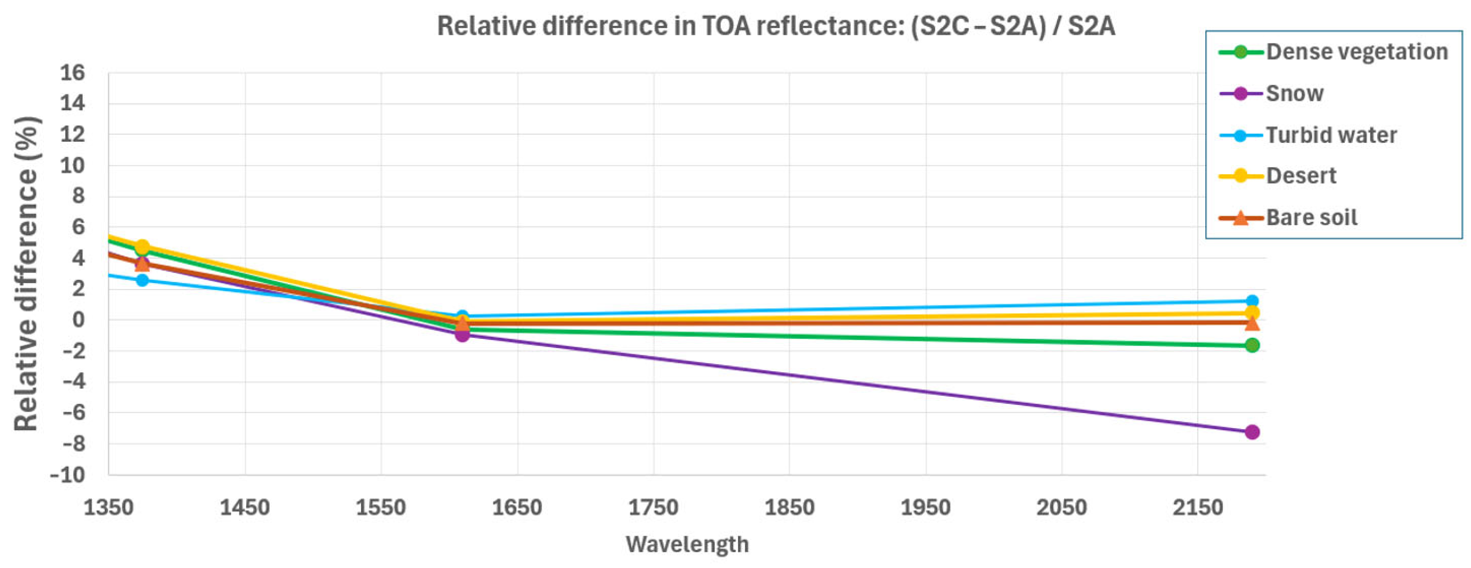
Figure 2. Relative spectral response functions for S2A (solid), S2B (dashed), and S2C (dotted) for VNIR spectral bands.
Remotesensing 18 01387 g002
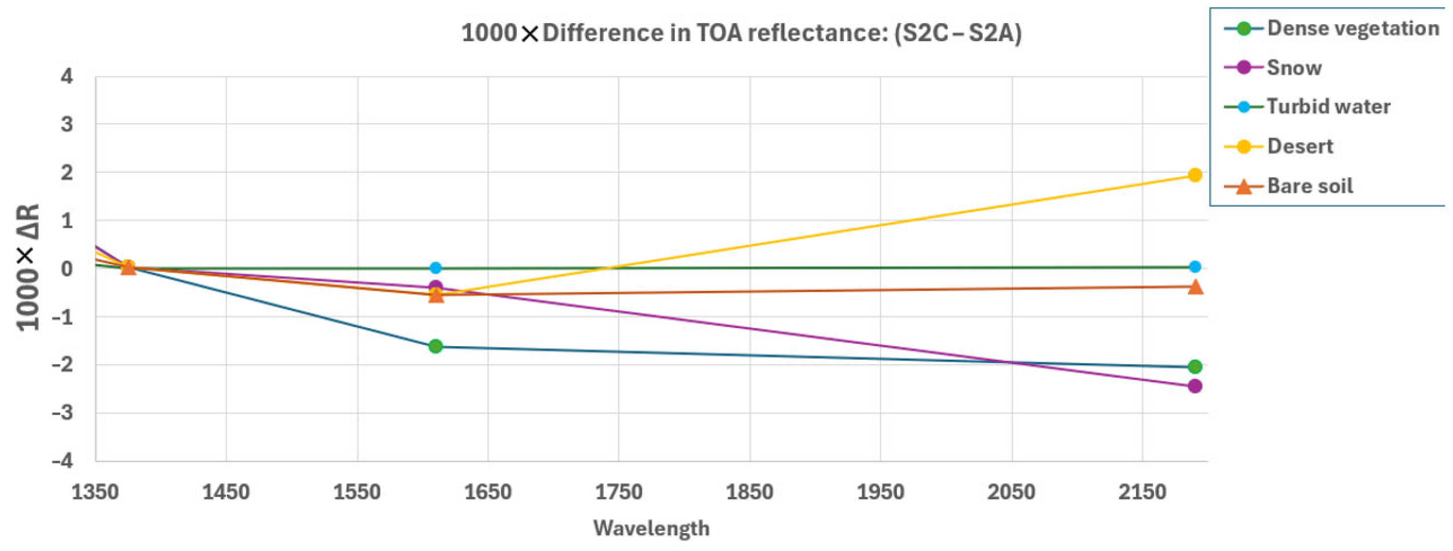
Figure 3. Relative spectral response functions for S2A (solid), S2B (dashed), and S2C (dotted) for SWIR spectral bands.
Remotesensing 18 01387 g003
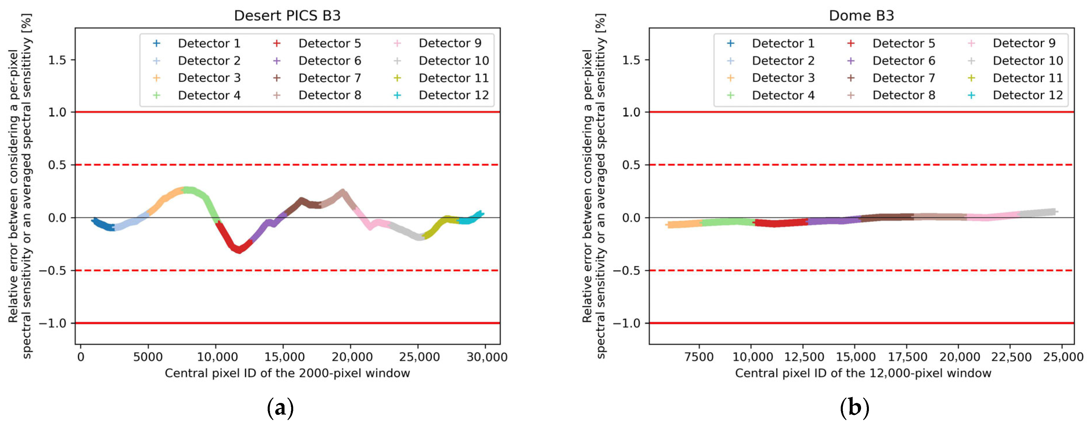
Figure 4. Flowchart of the radiometric calibration and validation activities performed in the present work.
Remotesensing 18 01387 g004
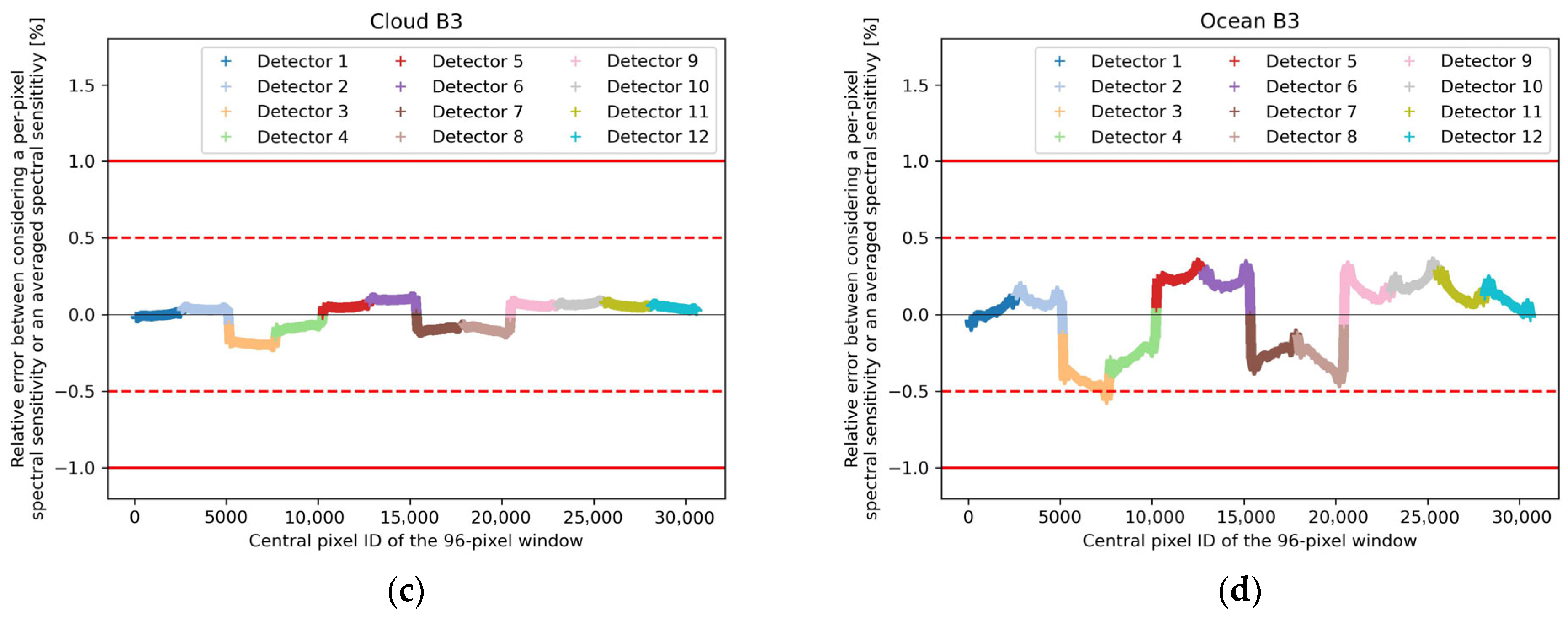
Figure 5. Desert PICS calibration dataset available for Sentinel-2C during the commissioning phase. Colored squares indicate the different sites, with the corresponding names shown in the legend. The CNES study includes all sites; the OPT-MPC analysis is focused on the CEOS sites. The number of products included in this assessment is indicated alongside each site name (e.g., Algeria-1: 3 products).
Remotesensing 18 01387 g005
Figure 6. Dome calibration dataset available for Sentinel-2C during the commissioning phase. Colored squares indicate the different sites, with the corresponding names shown in the legend. The number of products included in this assessment is indicated alongside each site name (e.g., Dome_1: 21 products).
Remotesensing 18 01387 g006
Figure 7. Ocean calibration dataset available for Sentinel-2C during the commissioning phase. Colored dots indicate different sites, with the corresponding names shown in the legend. The number of calibrated measurements and products included in this assessment as well as the detectors covered are indicated alongside each site name (e.g., AtlN: 727 calibrated measurements/3 products/detectors n°[1 2 3]).
Remotesensing 18 01387 g007
Figure 8. Geographical location of the DCC tandem products acquired by both Sentinel-2A (orange dots) and Sentinel-2C (blue dots) between October and December 2024. The CNES site is highlighted in green.
Remotesensing 18 01387 g008
Figure 9. Moon images acquired during the Sentinel-2C commissioning phase. The images are resampled to get a circular Moon disk, while the real acquisitions are elongated in the along-track direction.
Remotesensing 18 01387 g009
Figure 10. Mean radiance difference (S2C−S2A) versus mean radiance (S2A) for B02 (a), B04 (b), B06 (c) and B08 (d) for each detector. The dashed vertical black line shows the reference radiance Lref for each band. The twelve detectors are plotted with different colors and the average slope of linear trend of all detectors is displayed at the bottom of the figure. This plot highlights the linearity of the response and the low inter-detector dependence.
Remotesensing 18 01387 g010
Figure 11. Time evolution of absolute gains from Sun diffuser calibration per band, with respect to the first in-flight estimate on 14 September 2024. Top illustration is for VNIR bands. Bottom illustration is for SWIR bands.
Remotesensing 18 01387 g011
Figure 12. Change in equalization coefficients, expressed by the unitless Ra factor, as a function of pixel number for bands B06 (left) and B11 (right), between the Sun calibration on 20 November 2024, and the first in-flight calibration (on 14 September 2024). Equalization coefficients are more stable over time for VNIR bands such as B06 than for SWIR bands such as B11.
Remotesensing 18 01387 g012
Figure 13. Variation in equalization coefficients expressed by the unitless Ra factor as a function of pixel number over a yearly cycle, for the band B01 of MSI-C, using the on-ground characterization of the Sun diffuser BRDF (i.e., original BRDF). Each colored plot corresponds to an acquisition performed on a different orbit with a specific Sun azimuth angle (SAA). The Sun acquisition of orbit 862 is taken as the reference to estimate the change in equalization coefficients (Ra factor).
Remotesensing 18 01387 g013
Figure 14. Evolution of equalization coefficients expressed by the unitless Ra factor, as a function of pixel number for the B01 band, over a yearly cycle from September 2024 to September 2025 (exact dates are listed on top right), using the Sun acquisition on 1 October 2024 as reference. The top illustration shows the estimate of the Ra factor versus the pixel number using the original Sun diffuser BRDF (on-ground characterization). The bottom one illustrates the same estimates but using the refined BRDF (issued from in-flight Sun diffuser acquisitions with different yaw angles). The refined BRDF model provides more stable equalization coefficients.
Remotesensing 18 01387 g014
Figure 15. DIMITRI vicarious calibration results over desert sites as the ratio of the observed TOA-reflectance of the sensor to the TOA reflectance calculated by the PICS algorithm. (a) In blue, the calibrated sensor is Sentinel-2C/MSI and in orange, Sentinel-2A/MSI, using MERIS 3rd Reprocessing as the reference sensor; (b) direct comparison between Sentinel-2C and Sentinel-2A restricted to the tandem phase data using the double ratio technique, i.e., PICS products acquired quasi-simultaneously (within 30 s). Error bars show the standard deviation. The red solid and dashed lines represent the absolute radiometric uncertainty threshold (5%) and goal (3%) requirements of the Sentinel-2 mission, respectively.
Remotesensing 18 01387 g015
Figure 16. SADE/MUSCLE calibration results over desert sites. In blue, the calibrated sensor is Sentinel-2C and in orange, Sentinel-2A. Filled circles indicate a calibration result for which the spectral response correction is accurate; unfilled circles display results for which a strong spectral correction was required. The sensor taken as reference differs for each panel: (a) MERIS, (b) Sentinel-3 OLCI-B, and (c) LANDSAT-9. Panel (d) gives a direct comparison between Sentinel-2C and Sentinel-2A restricted to the tandem phase data, i.e., PICS products acquired quasi-simultaneously (within 30 s). The error bars provide the standard deviation of the results. The red solid and dashed lines represent the absolute radiometric uncertainty threshold (5%) and goal (3%) requirements of the Sentinel-2 mission, respectively.
Remotesensing 18 01387 g016aRemotesensing 18 01387 g016b
Figure 17. SADE/MUSCLE calibration results over dome sites. In blue, the calibrated sensor is Sentinel-2C and in orange, Sentinel-2A. Filled circles indicate a calibration result for which the spectral response correction is accurate; unfilled circles display results for which a strong spectral correction was required. The sensor taken as reference differs for each panel: (a) MERIS and (b) Sentinel-3 OLCI-B. Panel (c) gives a direct comparison between Sentinel-2C and Sentinel-2A restricted to the tandem phase data, i.e., PICS products acquired quasi-simultaneously (within 30 s). The error bars provide the standard deviation of the results. The red solid and dashed lines represent the absolute radiometric uncertainty threshold (5%) and goal (3%) requirements of the Sentinel-2 mission, respectively.
Remotesensing 18 01387 g017
Figure 18. DIMITRI calibration results over ocean sites. In blue, the calibrated sensor is Sentinel-2C and in orange, Sentinel-2A. The Sentinel-2C calibration dataset over the commissioning phase is very limited compared to the full-year Sentinel-2A dataset. The red solid and dashed lines represent the absolute radiometric uncertainty threshold (5%) and goal (3%) requirements of the Sentinel-2 mission, respectively.
Remotesensing 18 01387 g018
Figure 19. SADE/MUSCLE calibration results over ocean sites. In blue, the calibrated sensor is Sentinel-2C and in orange, Sentinel-2A. The Sentinel-2C calibration dataset over the commissioning phase is very limited compared to the full-year Sentinel-2A dataset. The error bars provide the standard deviation of the results. The red solid and dashed lines represent the absolute radiometric uncertainty threshold (5%) and goal (3%) requirements of the Sentinel-2 mission, respectively.
Remotesensing 18 01387 g019
Figure 20. Analysis of the temporal differences between DCC Sentinel-2A/Sentinel-2C tandem products: (a) histogram of the temporal differences between MSI-A and MSI-C sensing times; (b) product acquisition dates with regard to the commissioning phases, with the 30 s tandem period (blue bar) and MSI-C full acquisition plan period (red bar) highlighted.
Remotesensing 18 01387 g020
Figure 21. Relative difference between MSI-C and MSI-A reflectance indicator computed by the OPT-MPC DCC method for all bands except band 10, using tandem products acquired between October and December 2024. Error bars are a measure of the uncertainty taking into account statistical spread of the results and the uncertainty of the spectral band adjustment factors. Dotted, dashed and dash-dotted lines respectively represent zero, one and three percent relative difference with the reference.
Remotesensing 18 01387 g021
Figure 22. SADE/MUSCLE inter-band calibration results obtained on Deep Convective Clouds. In blue, the results correspond to Sentinel-2C and in orange to Sentinel-2A. The B04 (665 nm) is taken as the reference and the other points indicate the relative calibration of each band with regard to this reference. The error bars provide the standard deviation of the results. The red solid and dashed lines represent the absolute radiometric uncertainty threshold (5%) and goal (3%) requirements of the Sentinel-2 mission, respectively. The light red dotted line at ±1% was added to highlight the high spectral consistency for most bands.
Remotesensing 18 01387 g022
Figure 23. Sentinel-2C/MSI lunar irradiances compared to the LIME model per band for different Moon acquisitions during the Sentinel-2C commissioning phase. The red solid and dashed lines represent the absolute radiometric uncertainty threshold (5%) and goal (3%) requirements of the Sentinel-2 mission, respectively.
Remotesensing 18 01387 g023
Figure 24. Lunar delta gain phase angle dependency for different Moon acquisitions performed during the Sentinel-2C commissioning phase. The plot shows a decline in delta gain with increasing illumination phase angle for the band B06.
Remotesensing 18 01387 g024
Figure 25. ROLO-CNES lunar calibration results. Filled circles indicate that the results are within the validity domain of the model whereas empty circles indicate that the results include a model extrapolation, which may be less reliable. The red solid and dashed lines represent the absolute radiometric uncertainty threshold (5%) and goal (3%) requirements of the Sentinel-2 mission, respectively.
Remotesensing 18 01387 g025
Figure 26. Mean Sentinel-2C/Sentinel-2A radiometric gain ratios per band for 3 distinct surface types: bare soil (blue cross), water (green stars) and vegetation (orange dots). Error bars represent the standard deviation of the results across individual detector modules.
Remotesensing 18 01387 g026
Figure 27. Mean Sentinel-2C/Sentinel-2A gain ratios per band for bare soil pixels for 3 different times periods, starting with the 1st November in blue, the 7th November in orange, and the 14th November in green. Error bars represent the standard deviation of the results. Results are stable over time except for atmospheric bands B09 and B10.
Remotesensing 18 01387 g027
Figure 28. Synthesis of Sentinel-2C/Sentinel-2A inter-calibration gains per band measured by various methods. The colored solid lines indicate the different radiometric validation methods used while the dashed green line indicates the best estimate used for radiometric adjustment.
Remotesensing 18 01387 g028
Figure 29. DIMITRI cross-comparison of the Sentinel-2 constellation after the Sentinel-2C radiometric correction using the PICS double ratio technique. The red solid and dashed lines represent the absolute radiometric uncertainty threshold (5%) and goal (3%) requirements of the Sentinel-2 mission, respectively. The dotted red line emphasizes that all spectral bands are within 1% or better.
Remotesensing 18 01387 g029
Figure 30. SADE/MUSCLE cross-comparison of the Sentinel-2 constellation over PICS sites after the Sentinel-2C radiometric correction using Sentinel-2B as the reference. The error bars provide the standard deviation of the results. The red solid and dashed lines represent the absolute radiometric uncertainty threshold (5%) and goal (3%) requirements of the Sentinel-2 mission, respectively. The dotted red line emphasizes that all spectral bands are close to 1% or better.
Remotesensing 18 01387 g030
Figure 31. Cross-comparison of the Sentinel-2 constellation after the Sentinel-2C radiometric correction based on the OPT-MPC DCC method. The relative differences (MSI-A minus MSI-B and MSI-C minus MSI-B) of reflectance indicators are computed for all bands except band 10, using all products available between March and July 2025. Error bars are a measure of the uncertainty taking into account the statistical spread of the results and the uncertainty of the spectral band adjustment factors. Dotted, dashed and dash-dotted lines respectively represent zero, one and three percent relative difference with the reference.
Remotesensing 18 01387 g031
Figure 32. Reflectance of simulated surfaces as a function of the wavelength. The curves represent typical spectral signatures for snow (red), desert (blue), dense vegetation (green), turbid water (black), and bare soil (magenta).
Remotesensing 18 01387 g032
Figure 33. Absolute and relative difference (in %) of the TOA reflectance for MSI-C and MSI-A, expected above typical kinds of surface, for VNIR bands. The top illustration shows the relative differences. The bottom illustration shows the absolute differences in thousandths of reflectance.
Remotesensing 18 01387 g033
Figure 34. Same illustrations as Figure 33 but for SWIR bands.
Remotesensing 18 01387 g034aRemotesensing 18 01387 g034b
Figure 35. Evaluation of the SADE/MUSCLE results sensitivity to the in-swath spectral response variations for band B03 (561 nm). The different vicarious calibration methods involved in this study are analyzed: (a) the desert cross-calibration on small sites, (b) the dome cross-calibration on large sites, (c) the DCC inter-calibration, and (d) the absolute calibration on ocean sites. For each possible position of the vicarious calibration target across the swath (given on the abscissa), the graph provides the relative error between considering the real per-pixel spectral response or considering only an averaged spectral response. These errors are estimated by simulation. The solid red line indicates an acceptable uncertainty level of 1% and the dotted line indicates a goal uncertainty level of 0.5%.
Remotesensing 18 01387 g035aRemotesensing 18 01387 g035b
Figure 36. Repartition of the SADE/MUSCLE calibration results used for the Sentinel-2C/Sentinel-2A bias with regard to the vicarious target radiance for band B03 (561 nm). The L m i n and L m a x abscissae correspond to the dynamic range specified for the Sentinel-2 mission. The red solid and dashed lines represent the absolute radiometric uncertainty threshold (5%) and goal (3%) requirements of the Sentinel-2 mission, respectively. This figure indicates that the results are not affected by strong non-linear effects.
Remotesensing 18 01387 g036
Figure 37. Effect of a restricted time period on a Sentinel-2A/LANDSAT-8 cross-comparison computed on SADE/MUSCLE. Filled circles indicate a calibration result for which the spectral response correction is accurate; unfilled circles display results for which a strong spectral correction was required. The error bars provide the standard deviation of the results. The red solid and dashed lines represent the absolute radiometric uncertainty threshold (5%) and goal (3%) requirements of the Sentinel-2 mission, respectively.
Remotesensing 18 01387 g037
Table 1. Spectral information and associated resolution per band for S2A, S2B and S2C.
Band NumberBand Resolution (m)S2AS2BS2C
Equivalent Wavelength (nm)Bandwidth (nm)Equivalent Wavelength (nm)Bandwidth (nm)Equivalent Wavelength (nm)Bandwidth (nm)
160442.720442.220444.221
210492.764492.365489.065
310559.835558.935560.636
410664.630664.931666.530
520704.114703.815707.115
620740.514739.114741.115
720782.820779.720784.721
810832.8118832.9115834.6114
8a20864.720864.020865.620
960945.120943.220947.220
10601373.5301376.9301372.233
11201613.7881610.4931612.089
12202202.41792185.71812191.3182
Table 2. Main events during the Sentinel-2C in-orbit commissioning phase.
EventDate
S2C launch5 September 2024
S2A/S2C tandem30 October–19 December 2024
S2C yaw maneuver4 November 2024
S2C transfer to operation21 January 2025
S2A extension campaign13 March 2025
Table 3. Statistical results for the Ra factor for the Sun acquisition on 20 November 2024 in comparison with 14 September 2024.
MinMeanMaxStd
B010.9991.0001.0010.0004
B020.9990.9991.0000.0003
B030.9980.9991.0010.0005
B040.9970.9991.0000.0004
B050.9980.9991.0000.0003
B060.9980.9991.0000.0005
B070.9981.0001.0010.0004
B080.9980.9991.0010.0004
B8A0.9980.9991.0010.0004
B090.9970.9991.0000.0004
B100.9881.0001.0310.0028
B110.9931.0001.0230.0034
B120.9931.0001.0110.0012
Table 4. Synthesis of Sentinel-2C/Sentinel-2A inter-calibration coefficients (in %) assessed by different methods and best estimate based on all available results. The “st.d.” column provides the statistical uncertainty computed by the standard deviation of the results dataset; the “SBAF unc.” quantifies the uncertainty associated with the spectral band adjustment factor which is applied in some methods. Background colour is used to distinguish the different methods.
PICSPICSDCCTandemBest Estimate
CNES(Soil)
Gainst.d.Gainst.d.Gainst.d.SBAF unc.Gainst.d.Gain
B011.551.42.10.40.940.31.82.260.41.71
B022.831.53.60.22.740.31.82.020.22.80
B031.571.61.60.11.680.31.82.140.21.75
B041.621.01.60.12.120.31.52.310.21.91
B050.871.31.10.10.760.31.61.790.21.13
B061.800.720.12.340.31.82.200.22.08
B070.990.80.90.10.820.21.70.850.20.89
B081.351.11.70.11.30.21.71.360.31.43
B8A1.460.71.30.11.670.21.71.470.11.47
B092.170.61.72.17
B10
B111.60.31.880.53.41.560.51.68
B122.50.25.250.53.33.320.53.69
Table 5. Difference in simulated TOA reflectance (1000 × ΔR) for MSI-A and MSI-C, over the 5 types of surfaces, for the 13 spectral bands.
S2C−S2ADense
Vegetation
SnowTurbid
Water
DesertBare Soil
B1−0.90.8−1.00.0−0.5
B21.00.21.1−0.10.8
B3−0.7−1.30.30.5−0.2
B40.06.2−1.13.91.4
B516.68.49.06.42.7
B66.41.91.01.50.6
B7−3.8−6.9−1.7−2.8−1.2
B8−2.7−4.2−2.1−1.9−0.8
B8A0.6−0.4−0.30.40.3
B97.47.31.25.42.8
B100.00.00.00.00.0
B11−1.6−0.40.0−0.5−0.6
B12−2.0−2.50.01.9−0.4
Table 6. Statistics on central wavelengths (CWL) and full width at half maximum (FWHM) values for S2C—minimum, average and maximum values over all the pixels, range and standard deviation, per band.
CWL (nm)FWHM (nm)
MinAvgMaxΔStdMinAvgMaxΔStd
B01443.6443.9444.20.60.1116.019.720.64.60.91
B02488.3488.7489.20.90.1563.865.065.51.80.26
B03560.0560.5560.90.80.1533.835.035.51.70.31
B04666.2666.6666.90.60.1028.930.030.51.60.27
B05706.6707.1707.61.00.1814.715.115.50.80.22
B06740.6741.1741.40.70.1614.915.115.50.60.14
B07784.3785.1785.61.30.2119.520.020.61.10.32
B08842.1843.2844.32.30.4177.596.3111.634.17.93
B8A865.5865.9866.30.80.1619.019.920.51.50.31
B09947.2947.8948.31.20.2019.219.820.51.30.31
B101370.71372.41374.13.40.9132.732.933.40.70.14
B111609.81611.11613.13.30.7688.589.389.91.40.21
B122189.62192.32194.04.30.88179.0180.8183.14.10.50
Disclaimer/Publisher’s Note: The statements, opinions and data contained in all publications are solely those of the individual author(s) and contributor(s) and not of MDPI and/or the editor(s). MDPI and/or the editor(s) disclaim responsibility for any injury to people or property resulting from any ideas, methods, instructions or products referred to in the content.