


Highlights
The Cyclone Global Navigation Satellite System (CYGNSS) was launched in December 2016 and is designed to provide improved wind-speed observations over tropical and subtropical oceans. Part of the mission included developing an ocean surface heat flux product that used CYGNSS wind speeds to estimate air–sea interactions over these regions. This product has become a valuable resource for the community and continues to be refined, underscoring the importance of reliable observations of air–sea interactions.
What are the main findings?
- CYGNSS upgraded winds, replacing MERRA-2 with ERA5 for thermodynamic fields, and refined COARE processing have steadily enhanced the quality of CYGNSS-derived heat fluxes and substantially reduced product latency.
- Despite relying on reanalysis for thermodynamic variables (i.e., temperature and humidity), CYGNSS provides valuable flux information where in situ data are sparse, complementing other satellite missions and demonstrating the feasibility and utility of spaceborne air–sea interaction observations.
What are the implications of the main findings?
- Improved temporal resolution and reduced latency expand CYGNSS’s utility, enabling researchers to study better air–sea interactions that influence weather system development.
- The demonstrated value of CYGNSS strengthens the case for future missions capable of providing dedicated, improved spaceborne observations of air–sea interactions and marine boundary layer processes.
Abstract
The initial development of the Cyclone Global Navigation Satellite System (CYGNSS) Ocean Surface Heat Flux Product, shortly after the satellite mission began, quickly became a valuable tool for analyzing and monitoring latent and sensible heat fluxes over tropical and subtropical oceans. It helps improve understanding of their influence on tropical and extratropical cyclones, tropical convection, atmospheric rivers, and more. Since its first release, the product has been updated with new ancillary input data (such as temperature and humidity), algorithm adjustments to incorporate equivalent neutral winds from CYGNSS, and the addition of local solar time to support diurnal analysis. As a mature mission and data product, CYGNSS provides important climatological and long-term insights into the tropical and subtropical oceans, filling gaps where in situ observations and data from other remote sensing instruments are limited. This paper outlines the updates and changes made to the CYGNSS Fluxes since its inception, compares the current dataset with in situ data, and discusses CYGNSS’s long-term observations of ocean surface heat fluxes in the tropical and subtropical regions.
1. Introduction
Ocean surface latent heat flux (LHF) and sensible heat flux (SHF) facilitate the transport of heat and moisture between the ocean surface and the marine boundary layer (MBL). LHF and SHF can affect various weather and climate events, including tropical and extratropical cyclones [1,2], atmospheric rivers [3], and tropical systems/convection [4]. Given that LHF and SHF are directly influenced by surface wind speeds and by differences in humidity and temperature between the surface and the lower atmosphere [5], improvements in ocean wind speed measurements can help the scientific community better understand and estimate LHF and SHF. In situ observations have been and continue to be the standard for air–sea interactions but are often limited by both spatial and temporal resolution. While spaceborne instruments cannot directly measure surface heat fluxes, they can be used to measure the components used to estimate them, such as surface wind speed, temperature, and humidity. However, previous spaceborne instruments were limited in coverage, as polar-orbiting satellites often feature large gaps over the tropical and subtropical/lower extratropical regions, while precipitation-induced signal attenuation affected their observations.
The Cyclone Global Navigation Satellite System (CYGNSS) constellation was launched in December 2016 to provide improved ocean surface wind speed measurements over the tropical and subtropical oceans at higher temporal frequencies and under nearly all weather conditions [6,7]. As part of the mission’s initial objectives, an ocean surface heat flux product was developed; this data product uses CYGNSS’s Level 2 (L2) wind speed measurements, along with ancillary reanalysis data for temperature and humidity, to calculate LHF and SHF at every CYGNSS specular point observation [8] (hereafter C19).
While there are numerous methods for estimating LHF and SHF, the most common methods use bulk aerodynamic formulas, including the CYGNSS Ocean Surface Heat Flux Product (hereafter referred to as CYGNSS Flux(es)) [8]. These formulas, which relate the turbulent fluxes as functions of wind speed and air–sea thermodynamic differences, can be written as
Here, ρa is the air density at the surface [kg m−3]; Lv is the latent heat of condensation (2.5 × 10⁶ J kg−1); and cp is specific heat at constant pressure (1004 J K−1 kg−1). CDE and CDH are, respectively, the exchange coefficients of moisture and sensible heat [unitless]; U is the magnitude of the surface wind speed [m s−1], Ts and qs are temperature [K] and specific humidity [kg kg−1], respectively, at the surface, while Ta and qa are the same but at 10 m above the surface. When LHF and SHF are positive, energy is transported from the surface into the lower atmosphere, whereas negative fluxes indicate that energy is transported from the lower atmosphere into the surface.
Though CYGNSS provides a multitude of observations, the only data products it provides that could be used to estimate LHF and SHF at every specular point are its wind speed product [6,7]. As a result, the CYGNSS Fluxes uses ancillary reanalysis data for thermodynamic variables (i.e., temperature and humidity) to calculate LHF and SHF. Although observations of these thermodynamic variables from in situ and remote sensing platforms were available, the spatial and temporal scales of these observations were not consistent with CYGNSS’s observation locations and frequencies [8]. While dependent on reanalysis data, the CYGNSS Fluxes can provide detailed information on air–sea interactions throughout the tropical and subtropical oceans. As shown in C19, the CYGNSS Fluxes results showed that the product provided nearly full daily coverage of the tropical and subtropical oceans and had the potential to estimate LHF and SHF within and around tropical and extratropical cyclones. When validated with in situ buoy observations, while CYGNSS exhibited a negative bias at higher flux values (as CYGNSS wind speeds would underestimate higher wind speeds), there was good validation at lower surface heat flux values [8], indicating that its observations were representative of the air–sea interactions typically observed over these parts of the globe. As a result, CYGNSS has been used in a variety of applications since launch and has become a valuable tool for the scientific community.
Within extratropical cyclones (ETCs), CYGNSS has been shown to provide valuable observations of surface heat fluxes during ETC development in the lower midlatitudes (30–40° in both hemispheres), especially along western boundary currents [9]. Additionally, when compositing CYGNSS’s ETC observations, one can observe the evolution of LHF and SHF between the developing, intensifying, and dissipating phases [10]. These composites of CYGNSS observations also showed clear correlations between LHF/SHF strength in the post-cold frontal sector and precipitation rates, ascent strength, and cloud thickness in the frontal regions of ETCs [11]. With atmospheric rivers (ARs), CYGNSS has been able to show that the surface moisture and heat source for ARs are typically located further away (i.e., not localized) [12], and with many ARs, the strongest surface heat fluxes are typically just outside and ahead of the AR as it develops and matures [13]. During tropical cyclone formation, CYGNSS Fluxes have shown enhanced surface heat fluxes within the core of a developing cyclone [14]. Additionally, CYGNSS Fluxes have shown correlations between surface heat fluxes and precipitation in tropical convection [15], their role in precipitation propagation in the Tropical Eastern Pacific Ocean [16], and how Madden–Julian Oscillation (MJO) events propagating through the Maritime Continent (MC) exhibit positive LHF anomalies [17]. These are just a few examples of how CYGNSS Fluxes have been used to help the scientific community better understand the role of air–sea interactions in Earth’s weather and climate. Additionally, the CYGNSS Fluxes have been independently validated by other scientists and researchers [18,19], demonstrating that they are a viable tool for the scientific community to better understand how surface processes contribute to weather and climate systems across all length and timescales.
Since the initial release of the CYGNSS Fluxes, various updates have been made to the product. This has included incorporating the latest L2 CYGNSS wind speed products, changing the ancillary reanalysis dataset to one with higher resolution and reduced time lag, changing how the reanalysis data are matched/interpolated with the CYGNSS specular points, and modifying the algorithm used to estimate LHF and SHF by accounting for the equivalent neutral winds produced by CYGNSS. Since their initial release, changes to the CYGNSS Fluxes have affected the results of LHF and SHF estimated by CYGNSS; however, there has been no comprehensive write-up or publication of these changes outside the updated user guides issued when a new product is released. This brief paper aims to describe and discuss changes in the CYGNSS Fluxes over the years, quantify the accuracy of the latest product using in situ observations from buoys, and showcase some of the capabilities of the CYGNSS Fluxes with nearly 7 years of data as a mature mission and data product.
The paper is structured as follows: Section 2 describes the updates to the input data and changes to the algorithm used to estimate the CYGNSS Fluxes. Section 3 will highlight comparisons to buoy data and discuss how they align with the results presented in C19. Section 4 will demonstrate the latest CYGNSS Flux observations and capabilities of a mature mission. Section 5 and Section 6 will have the discussion and conclusions, including future directions the CYGNSS Fluxes might take.
2. Data and Algorithm Updates
The following section provides a brief overview of the CYGNSS mission, the CYGNSS Flux algorithm, and the validation process using buoy data; however, the focus will primarily be on updates to the CYGNSS Fluxes since the initial product. For detailed descriptions of the CYGNSS satellites, the basis of the CYGNSS Flux Algorithm, and the methods for CYGNSS validation using buoy data, refer to previous publications [7,8,20,21,22]. The latest CYGNSS Fluxes (SDR V3.2) currently incorporate the L2 SDR V3.2 wind speed product from CYGNSS. The reanalysis data used for the CYGNSS Fluxes is ERA5, previously MERRA-2, given its improved horizontal resolution and reduced time lag. Additionally, adjustments to the algorithm used for the CYGNSS Fluxes have been made, including a more robust method for interpolating reanalysis data to the CYGNSS specular points and adjustments to account for equivalent neutral winds from CYGNSS. All of these are summarized in the following subsections.
2.1. CYGNSS Mission Overview
The Cyclone Global Navigation Satellite System (CYGNSS) was launched on 15 December 2016; it originally consisted of eight small satellites with a 35° orbital inclination, selected to maximize the observation of ocean surface wind speeds over the tropical and subtropical oceans where most tropical cyclones develop [6]. It accomplishes this by using Global Navigation Satellite System-Reflectometry (GNSS-R), which measures two signals from existing Global Positioning System (GPS) satellites: the direct signal from a zenith antenna and the reflected GPS signal from the ocean surface via two downward-pointing antennas at each observatory, acting as specular points [6,7]. The surface wind speed is estimated from the reflected GPS signal by using the Delay Doppler Map (DDM), the average reflected power from the DDM (DDMA), and its Leading-Edge Slope (LES). Additionally, the direct signal from GPS satellites is used to determine signal power, enabling calibration of the estimates.
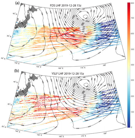
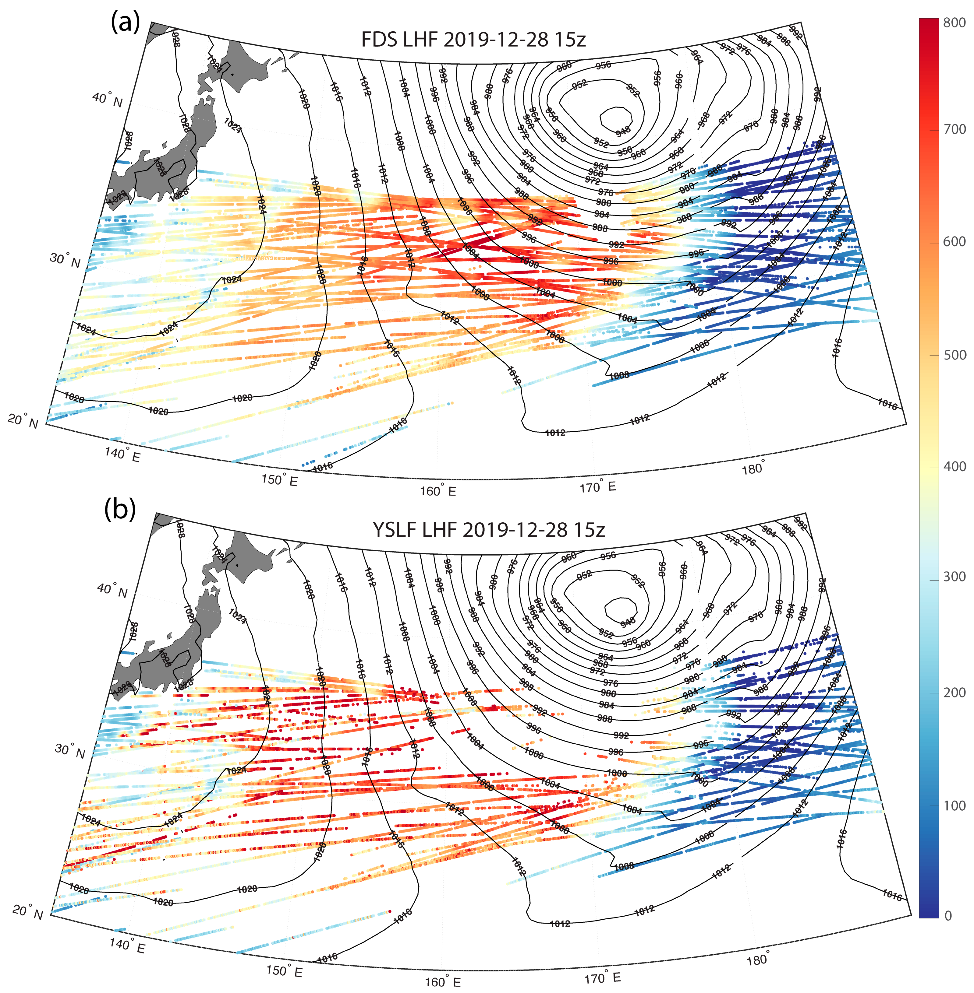
There are two concurrent wind speed measurements produced by CYGNSS within each product: Fully Developed Seas (FDS) and the preliminary Young Seas with Limited Fetch (YSLF). FDS assumes that the sea state is in equilibrium with the wind speed and is reliable for wind speeds under 20–25 m/s [7,22]. However, in high-wind situations, users are recommended to use the preliminary YSLF wind speeds, as this wind speed product does not assume that the sea state and local winds are in equilibrium. The preliminary YSLF winds are primarily used in CYGNSS’s Tropical Cyclone-centered projects and the Level 3 merged wind-speed product [23] but can also be used independently. Additionally, while time averaging is applied to overlapping specular points in FDS, it is not applied to the preliminary YSLF product to preserve individual specular-point wind speed data. While this often yields noisier results, it also yields more accurate wind speed observations at higher wind speeds. The CYGNSS fluxes use both the FDS and YSLF wind speeds, yielding FDS- and YSLF-based estimates of the LHF and SHF. However, because the CYGNSS algorithm is only validated for wind speeds up to 25 m/s, any specular points that meet those conditions are flagged for quality control and will be filtered out when the flags are applied. This is shown in Figure 1, which plots the LHF values from the SDR V3.2 product, estimated using the FDS and YSLF products, for an ETC in the Western Pacific Ocean off the coast of Japan on 28 December 2019 at 15:00 UTC. The FDS LHF values show a more uniform profile, with values exceeding 700 W m−2 (Figure 1a). A small section near the core of the ETC is excluded because it was filtered out by the quality control flags. When the LHF is estimated using the preliminary YSLF winds (Figure 1b), one notices that the LHF values are higher and less uniform because the YSLF product preserves individual specular-point wind speeds. However, because the YSLF winds are meant for higher wind speeds and therefore produce higher wind speed values, this leads to not only higher LHF values but also more specular points being filtered out by the quality control flags due to the CYGNSS Fluxes only being validated up to wind speeds of 25 m/s [8]. While the data from those specular points are still available in the product, users are advised to use caution when using this data and to apply the quality flags, as we cannot accurately validate these values.
Figure 1.
CYGNSS LHF observations [W m−2] from the FDS product (a) and the YSLF product (b) of an Extratropical Cyclone in the Western Pacific on 28 December 2019 at 15:00 UTC. Mean sea level pressure [hPa, black lines] indicates the location of the cyclone. Given that the YSLF wind speeds are higher, the flux values tend to be higher. However, since the CYGNSS Fluxes are only validated for wind speeds up to 25 m/s, many of the specular points are filtered out in the YSLF product.
Two wind speed products are produced by CYGNSS and used for the CYGNSS Fluxes: Science Data Record (SDR) and Climate Data Record (CDR). The SDR-retrieved wind speeds are available at every specular point (FDS and YSLF) and are calibrated using a stand-alone algorithm based on CYGNSS engineering data. The CDR product will use SDR winds and apply a trackwise correction algorithm similar to those previously used [24]. To summarize, CYGNSS measurements often produce “tracks” of consecutive specular points (as seen in Figure 1). To minimize the artifacts, overlapping specular points within the tracks are averaged on a 25 km grid, while low-quality observations are excluded. A boxcar smoothing window is then applied to the gridded tracks to reduce large fluctuations between adjacent samples. Co-located wind speed estimates from ERA5 and significant wave height from WaveWatch3 are then used to train the data [7,24]. Since overlapping specular points are averaged into a single specular point, the CDR products have fewer specular points than the SDR products [7]. When the CYGNSS Fluxes were initially released, only SDR products were available. Since then, CDR products for the CYGNSS mission have been introduced, and subsequent CDR CYGNSS Flux products have been created. It is generally recommended that users utilize SDR products for individual storms and case studies, while CDR products are used for climatological studies and composite analysis; however, SDR can also be used for these purposes. At the time of writing, the latest SDR version (3.2) has been released [25], but subsequent CDR products are still in development and are expected to improve on the current CDR version (1.2). Therefore, the results shown in this paper will only utilize SDR V3.2 of the CYGNSS Fluxes [26].
Previous CYGNSS wind speed products (as well as CYGNSS Fluxes) were available starting from March 2017, when the CYGNSS science mission initially began. However, beginning with CYGNSS Wind Speed Products SDR V3.0 and CDR 1.1 (SDR V2.0 and CDR V1.1 for the CYGNSS Fluxes), data were available from August 2018 to the present. This is due to an onboard calibration issue that was not resolved until the Summer of 2018, and data before this timeframe could not be retroactively calibrated correctly [7]. As a result, the newer CYGNSS wind speed and flux products began on 1 August 2018. Meanwhile, older CYGNSS products retain data from March 2017 to July 2018; however, users are not recommended to use this data alongside newer data due to calibration issues and possible errors in these products that have been resolved in the latest products.
2.2. ERA5 Reanalysis Data
The initial CYGNSS Fluxes used NASA’s Modern-Era Retrospective Analysis for Research and Applications, Version 2 (MERRA-2) [27] reanalysis data to complement CYGNSS wind speed observations and estimate LHF and SHF. Since CYGNSS only provides wind speed, estimates of LHF and SHF require surface and near-surface/lower boundary-layer thermodynamic variables (i.e., humidity and temperature). Reanalysis data are used because they provide consistent global estimates. While other satellite measurements were considered, gaps between their observations and CYGNSS could have led to inconsistent and inaccurate estimates of LHF and SHF, especially in and around rapidly evolving systems. Since its initial release, updated versions of the CYGNSS Fluxes, beginning with CDR V1.1 [28], have used ECMWF Reanalysis, Version 5 (ERA5) [29]. The switch was primarily made due to ERA5’s higher spatial resolution (0.25° × 0.25°, compared to 0.5° × 0.625° with MERRA-2) and significantly shorter latency (1 week compared to 1–2 months with MERRA-2), allowing CYGNSS Fluxes to be produced more rapidly. Additionally, previous studies have shown that ERA5 performs similarly to MERRA-2 [30,31,32]. However, while there were some improvements to the CYGNSS Fluxes due to ERA5, most improvements were related to the improved wind speed observations. Nevertheless, the enhanced resolution and latency have made the CYGNSS Fluxes more reliable.
Similarly to the MERRA-2 data originally used [8], the data are available hourly and have similar inputs (i.e., surface/skin temperature, air density, surface pressure), though there were some differences. In MERRA-2, air temperature and specific humidity were provided at 10 m, while ERA5 provides air temperature and dew point at 2 m. To apply the ERA5 variables to the algorithm used by the CYGNSS Fluxes (COARE 3.5 [33], discussed in the following section), we use dew point and air temperature to compute the vapor pressure and saturation vapor pressure, respectively. The ratio of the vapor pressure to the saturation vapor pressure (multiplied by 100%) is the relative humidity, which is then used to calculate the saturation specific humidity. Then, within COARE, it estimates the temperature and humidity at 10 m using the 2 m variables and the Monin–Obukhov Similarity Theory (MOST).
2.3. Algorithm Updates
Previously, the reanalysis data were matched to the CYGNSS specular point observations using a nearest neighbor method; the grid point closest to the specular point in time and space was used. However, subsequent versions have matched the reanalysis data to CYGNSS specular points using a tri-linear interpolation method to provide more accurate estimates for temperature and humidity. The matchup method initializes a regular-grid interpolator object using ERA5 (formerly MERRA-2) data in three dimensions: 2 m dew point temperature, 2 m temperature, air density over the oceans, boundary layer height, skin temperature, and surface pressure, all at their respective latitudes, longitudes, and times. The interpolator takes CYGNSS data dimensioned by latitude, longitude, and time as input and uses trilinear interpolation to return ERA5 model data values at each CYGNSS three-dimensional point. Essentially, ERA5 model data is re-gridded to the CYGNSS 3D grid.
The CYGNSS Fluxes continue to utilize the COARE 3.5 algorithm [33] for their LHF and SHF estimates. The COARE 3.5 algorithm was slightly modified for use with CYGNSS Fluxes to account for the fact that the latest CYGNSS wind speeds represent stability-independent, or equivalent neutral, winds rather than actual winds. The modifications to COARE were similar to those discussed in previous publications [34,35], addressing stability-dependent biases between equivalent neutral winds and actual winds. This includes evaluating the friction velocity (u*) and surface stress (τ) with the neutral drag coefficient rather than the stability-dependent drag coefficient (CDE and CDH from Equations (1) and (2), respectively). These adjustments improved the accuracy of CYGNSS-derived sensible and latent heat-flux estimates in comparison to buoy-based bulk fluxes, yielding a bias reduction of 10–20 W/m2 for latent heat-flux and 1–2 W/m2 for sensible heat-flux [35]. The inputs to the COARE 3.5 algorithm remain the CYGNSS wind speeds and the interpolated ERA5 data. Using the COARE algorithm, LHF and SHF are estimated at every specular point, with FDS and preliminary YSLF winds, in both the SDR and CDR versions. However, given that fluxes from COARE 3.5 are only validated to wind speeds up to 25 m/s [33], and CYGNSS’s YSLF products are now only recommended for cases with high wind speed (>20–25 m/s) [7], the validation results shown here, as well as any results, in the following sections will utilize the FDS CYGNSS Fluxes that use the FDS wind speed estimates. The YSLF product from CYGNSS Fluxes is still available and includes quality-control flags for high-wind-speed conditions. Users are advised to proceed with caution when these quality control flags are present, as we cannot accurately validate these values.
The latest CYGNSS Fluxes product (SDR V3.2) includes the estimated local solar time (LST) for every specular point. Given CYGNSS’s non-sun-synchronous orbit, its data can be used for diurnal studies, case studies for specific regions, and climatological/composite analysis across the entire mission. LST is estimated using the date, longitude, and UTC of every specular point using the PyEphem Python library (version 3.7.6.0, https://rhodesmill.org/pyephem/, accessed on 1 February 2023). The following description offers a basic explanation of how LST is calculated through this function. The average time of a solar day (the time between each solar noon) across a year, and outside of the polar regions, is about 24 h (86,400 s). However, due to Earth’s tilted axis and elliptical orbit around the Sun, the time between solar noon varies throughout the year; solar days are longer around December and January when the Earth reaches Perihelion around the first week of January, with the shorter solar days occurring around June and July as Aphelion occurs around the first week of July [36]. To account for its impact on LST, the Equation of Time (EoT) is used to estimate how many seconds are needed to be adjusted every day in the following equations:
where DoY is the day of the year, ranging from 1 to 365 (366 for leap years), and the EoT output units are in minutes. The results of Equation (2) lead to the amount of time that needs to be subtracted or added to account for Earth’s relative position to the sun (tilt and orbit), as demonstrated in the Supplemental Files for this paper (Figure S1). EoT is then used to estimate the Time Correction (TC, Equation (3)) as a function of longitude. From there, TC is used, along with UTC recorded at the specular point, to estimate the LST of the observation. Since CYGNSS records UTC rather than the local time zone, further adjustments are not needed. This is done at every specular point using the functions mentioned above, allowing diurnal analysis to be performed more easily in certain parts of the globe. Additionally, since the number of specular points in the CYGNSS Fluxes matches their corresponding CYGNSS L2 wind speed products, the LST produced within the CYGNSS Fluxes can be used for the CYGNSS wind speed products.
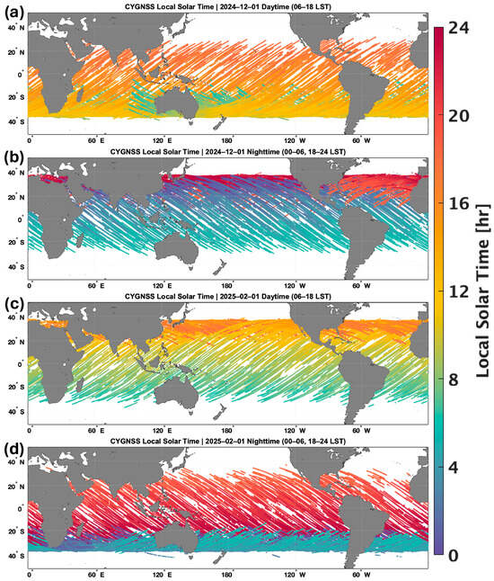
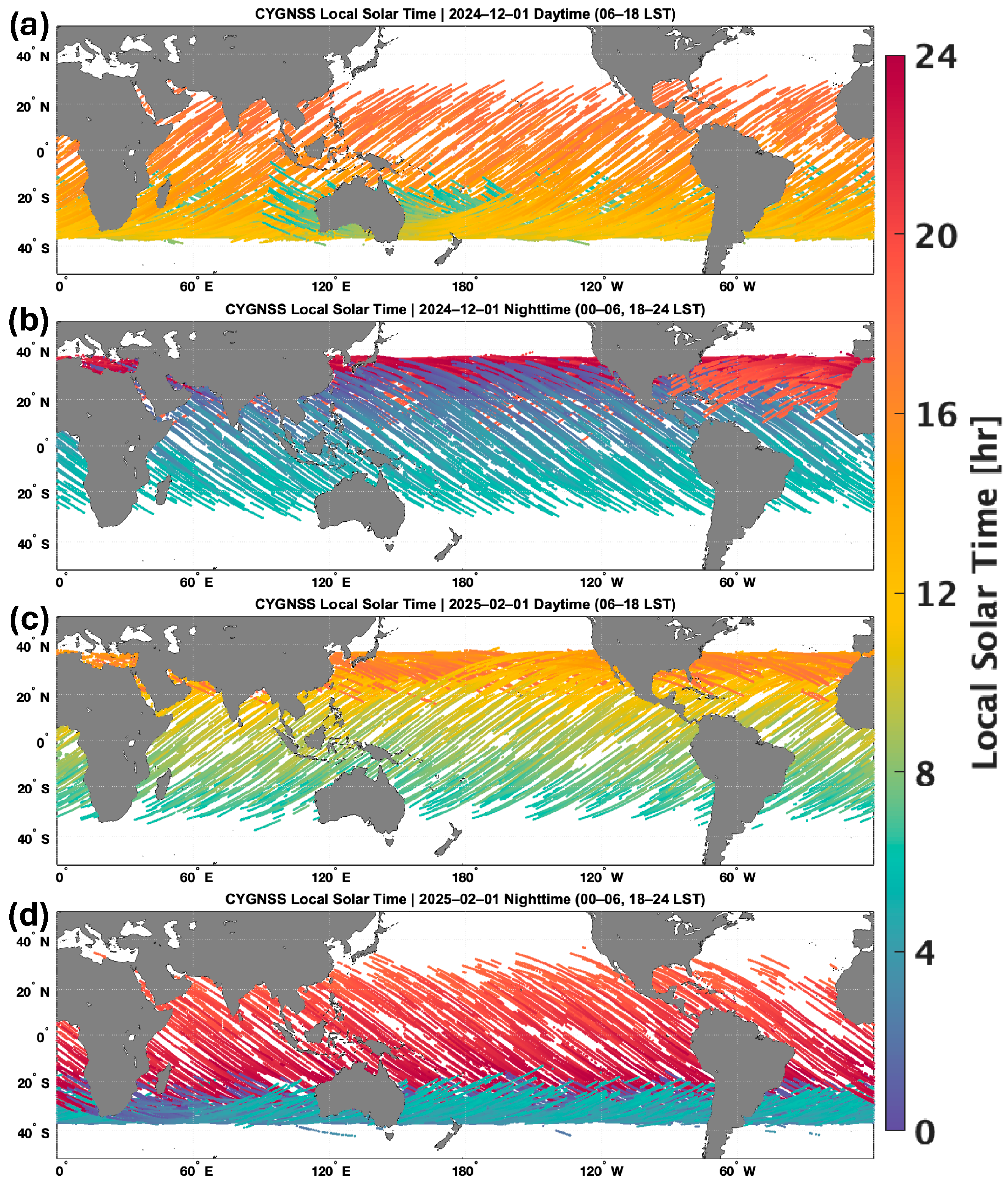
Figure 2 shows the LST of CYGNSS observations across two days, two months apart (1 December 2024 and 1 February 2025). The figures for each day are split into 12 h increments to best show CYGNSS’s diurnal observations: daytime (0600-1800 LST) and nighttime (1800-0600 LST). On both days, one can see that areas closer to the equator are more likely to have multiple sets of CYGNSS observations in a single day, such as over the Eastern Tropical Pacific Ocean, where CYGNSS observations occurred before 0600 and 1800 LST on 1 December (Figure 2a,b). Areas in the subtropics near the edge of CYGNSS’s range are more likely to have their measurements once a day but will cover a few hours (similar to what was seen in previous results [37]). However, because of CYGNSS’s non-sun-synchronous orbit, the LST of these observations changes throughout the year and can vary within a short time frame. In this example, observations on the north edge of CYGNSS’s range on 1 January are around 0800 LST (i.e., morning after sunrise). Yet, one month later, on 1 February, the observations are made after 1600 LST (i.e., in the afternoon, during sunset) (Figure 2c). While one cannot efficiently utilize CYGNSS observations for diurnal analysis over shorter periods, or specific case studies, in the subtropics and lower midlatitudes, it is possible at larger/climatological time scales and composite analyses of multiple weather events, such as extratropical cyclones and atmospheric rivers.
Figure 2.
Local Solar Time (LST) of CYGNSS specular point observations across two days, two months apart: 1 December 2024 (a,b) and 1 February 2025 (c,d). For clarity, the LST of the observations is split into 12 h intervals: daytime (a,c) and nighttime (b,d). CYGNSS’s orbit enables daily diurnal observations in the tropical regions. While observations in the subtropical regions tend to occur at approximately the same time each day, because of CYGNSS’s non-sun-synchronous orbit, the timing of these observations shifts, allowing diurnal analysis at climatological scales.
3. Updated Buoy Validation Results
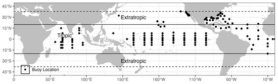
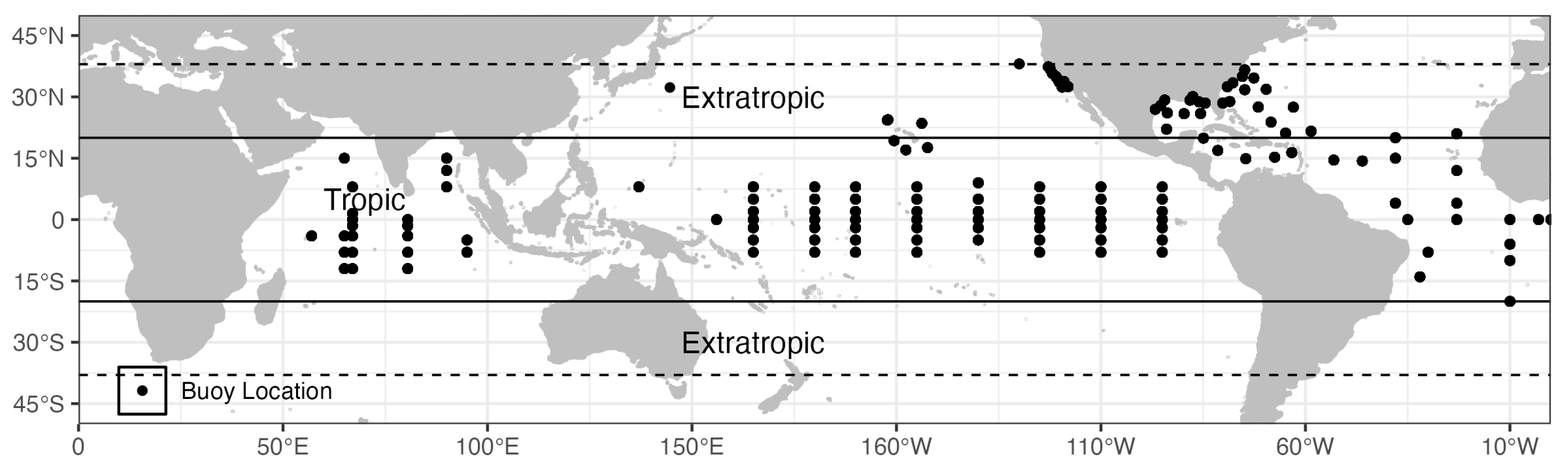
Similarly to C19, the CYGNSS Fluxes are compared to buoy data across the tropical and subtropical oceans within CYGNSS’s range (Figure 3). The buoys used for these comparisons, such as those from the National Data Buoy Center (NDBC) [38], Tropical Atmosphere Ocean Array (TAO) [39], the Prediction and Research Moored Array in the Tropical Atlantic (PIRATA) [40], and the Kuroshio Extension Observatory (KEO) [41], do not measure LHF and SHF directly but do measure wind speeds, temperature, and humidity, which can be directly inputted into the same COARE algorithm that has been utilized for the CYGNSS Fluxes, allowing for a direct comparison and validation of the data product. The buoy data can be accessed publicly through the National Oceanic and Atmospheric Administration (NOAA) and are compared using the same methods shown in C19 and the latest CYGNSS wind speed validation [20]. Overall, a similar number of buoys were used for these matchups as in C19, and the aggregated data totaled over 100,000 matchups (compared to ~21,000 in C19) after applying the CYGNSS quality flags. Additionally, for this comparison, we conduct a separate analysis focusing on tropical regions (~±20° latitude) and the subtropical/lower midlatitude region within CYGNSS’s range (~20–40° in both hemispheres) to better evaluate CYGNSS’s performance in these regions. Here, we have approximately 53,500 comparisons in the tropical regions with 58,000 in the subtropical regions (Table 1).
Figure 3.
Location of the collocated buoys incorporated from August 2018 to December 2023. The dashed line marks the extent of CYGNSS’s typical range (±38° latitude), though occasional (but sparse) observations may occur poleward of these lines. The solid black line divides the buoys between tropical locations (~±20° latitude) and the subtropical/extratropical regions (~20–40° in both hemispheres) for the analysis shown in Figure 4 and Table 1.
Table 1.
Statistics from the buoy comparisons shown in Figure 4 for LHF (left 3 columns) and SHF (right 3 columns) across all buoys (left), the extratropics (ET, middle), and the tropics (right), as defined by Figure 2. The statistics shown, from top to bottom, are the Root Mean Square Difference (RMSD), bias (μ), number of samples (N), and the correlation (r).
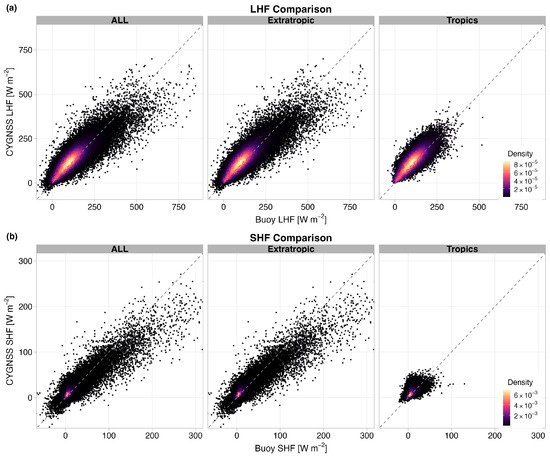
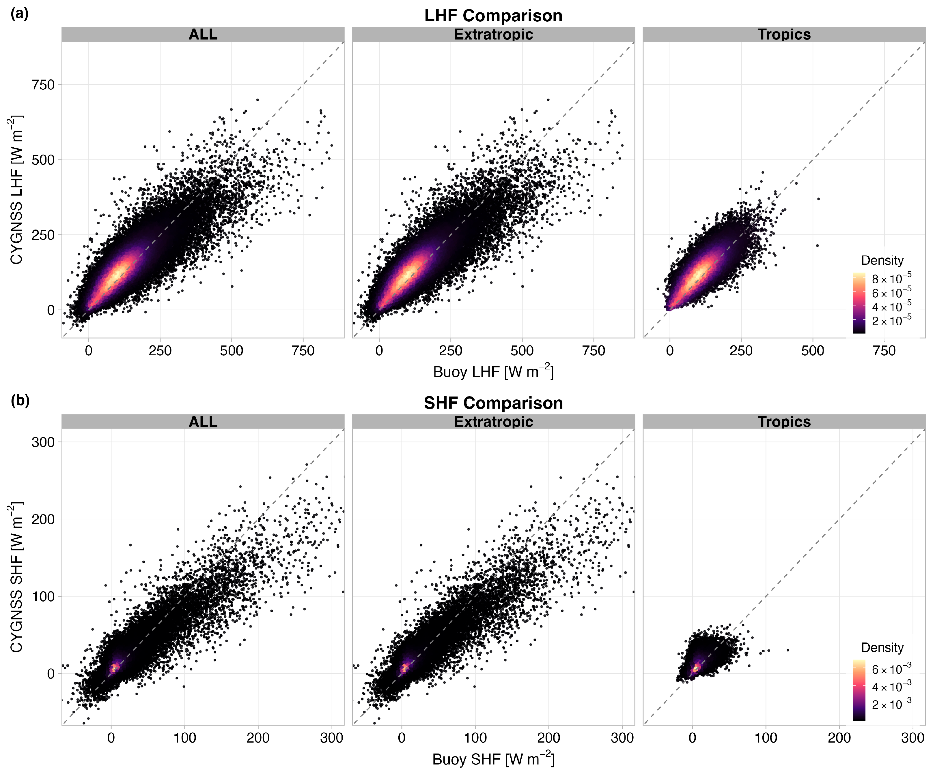
In these comparisons with buoy data (Figure 4 and Table 1), we observe similar trends in the latest CYGNSS fluxes, with slight improvements in the overall statistics. In both LHF and SHF, the majority of the CYGNSS Fluxes are along the one-to-one line with the buoy flux estimates, though there is a slight overestimate of LHF and SHF with CYGNSS at these values compared to the buoy data. Additionally, at higher LHF values (primarily in the subtropical regions, as will be discussed in Section 4), while comparisons show greater scatter, they are relatively evenly distributed around the 1-to-1 line, with a slight underestimation relative to buoy data. In the original data product [8], nearly all CYGNSS Fluxes at higher values were underestimated relative to the buoy data. However, with SHF, we observe a similar bias, albeit with higher values and a far greater number of data points than with C19.
Figure 4.
Two-dimensional density plot for collocated CYGNSS and buoy surface latent (a) and sensible (b) surface heat fluxes. On the left are the comparisons with buoys across the whole CYGNSS domain, the middle shows those in the tropical regions (~±20° latitude), while the right plots are comparisons in the subtropical and lower midlatitude regions of CYGNSS’s range (~20–40° in both hemispheres), as defined in Figure 2. The dotted line indicates the 1-to-1 line.
Due to the sparse availability of validation data across large portions of the global ocean and their non-uniform distribution that were available throughout CYGNSS’s entire mission so far (e.g., in the Southern Hemisphere and within western boundary current regimes), the present analysis does not provide a globally representative assessment of flux errors in these key regions. Nevertheless, buoy comparisons in extratropical regions from KEO and NDBC show promising results, with room for improvement. Additionally, while high-wind-speed events, such as tropical cyclones, do occur in tropical regions, quantifying the fractional contribution of tropical cyclones to the annual tropical latent and sensible heat flux budgets and isolating the event-specific impact of humidity errors on those fluxes would require a dedicated storm-composite analysis with collocated thermodynamic validation. This remains an important area for future research. Furthermore, many of those observations would be filtered out due to CYGNSS’s quality control flags (as shown in Figure 1).
While the statistics from Table 1 appear to show results similar to or worse than those in C19, it should be noted that the buoy data used for the initial validation were subjected to a stricter quality control criterion. This included excluding coastal observations, thereby limiting wind speeds to below 11 m/s [8]. Additionally, there is only a 4-month overlap between the two datasets (August 2018–January 2019), resulting in limited points of comparison. However, updates to the COARE algorithm have led to improvements in CYGNSS Fluxes in areas of high instability, such as the Western Boundary Currents (i.e., the Gulf Stream and Kuroshio Current/Extension) and the Arabian Sea [35]. In areas of higher instability, when adjusting the COARE 3.5 algorithm to factor in the equivalent neutral winds from CYGNSS [34], biases are significantly reduced, and RMSD values compared to buoy data are lower [35]. While the overlap values compared to the original CYGNSS fluxes may appear worse [8], these improvements in key areas will make the product more useful for case studies and climatological analyses for extreme weather and climate events.
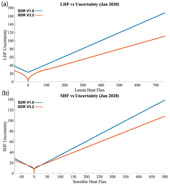
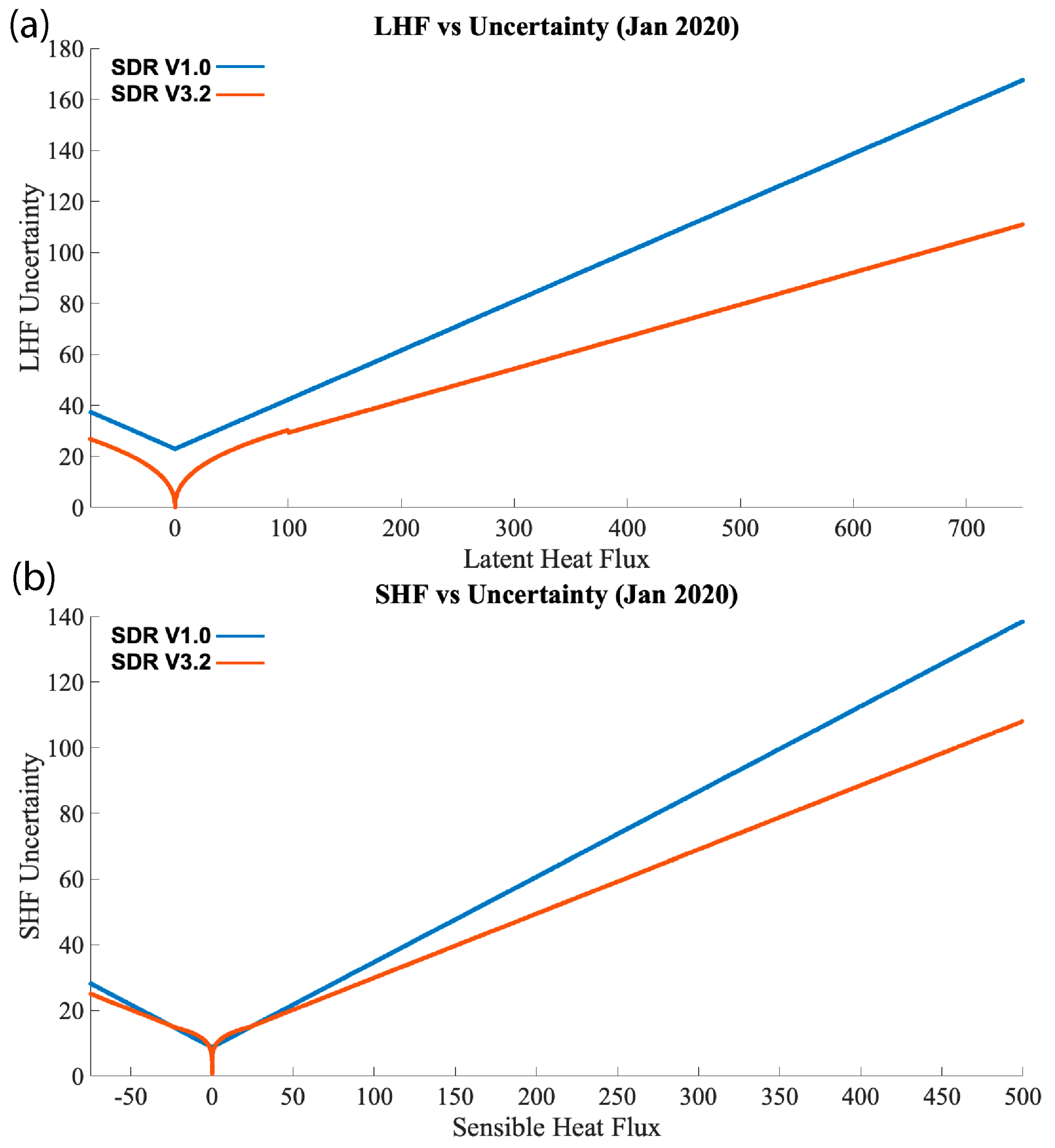
While the comparisons with buoys are similar to previous results, the uncertainty of the CYGNSS Fluxes has generally improved, primarily due to improvements in the wind speed product’s uncertainty. Figure 4 shows the uncertainty from the SDR V1.0 product (blue) and the latest SDR V3.2 product (orange) for both LHF (Figure 5a) and SHF (Figure 5b). While the SDR V1.0 product was retired in 2020, there were a few months where the two products overlapped, providing a chance for some direct comparisons. Here, uncertainties are plotted from all January 2020 files. These uncertainties come directly from the SDR V1.0 and V3.2 products and are calculated using the same method as described in Section 6 of C19, and then calculated as a function of LHF and SHF based on a best-fit model [8,25] in order to be able to estimate the uncertainties quickly for every file of the data product. The initial release used a simple linear fit for the uncertainty at all fluxes, but later releases, including SDR V3.2, use a logarithmic best-fit for LHF values between −100 to 100 W m−2 and −25 to 25 W m−2 for SHF. An example of how these were determined is shown in the Supplemental Materials (Figure S2). As shown in the uncertainty plotted as a function of LHF and SHF (Figure 5), there was a significant reduction in uncertainty for both LHF and SHF. This difference becomes more pronounced at higher flux values. Additionally, including logarithmic uncertainty functions at lower values better reflects the uncertainties at those values. For LHF, had a linear best fit function been used for all values, the LHF uncertainty within ±100 W m−2 would have been less than that in SDR V1.0. For SHF, the values within ±25 W m−2 were similar (or even slightly greater than) to the uncertainties in SDR V1.0, likely due to SHF being less dependent on wind speed at lower values (so the improved CYGNSS wind speeds had a small impact). Nevertheless, we see improvements at higher SHF values.
Figure 5.
The uncertainty of the CYGNSS Fluxes, plotted as a function of LHF (a) and SHF (b), directly from the CYGNSS Flux products (blue: SDR V1.0; orange: SDR V3.2) for one month of data where the two products overlapped (January 2020). A linear best-fit line was used to determine the uncertainty function for SDR V1.0, values above 100 (less than −100) W m−2 for LHF in SDR V3.2, and values above 25 (less than −25) W m−2 for SHF in SDR V3.2. In SDR V3.2, for LHF values between −100 and 100 W m−2 and SHF between −25 and 25 W m−2, a logarithmic function was used to determine the uncertainty function. Plots used to estimate the best-fit equations are shown in the Supplemental Material (Figure S2).
4. Updated CYGNSS Flux Observations and Results
The CYGNSS mission can provide nearly complete daily coverage over the tropical and subtropical oceans. By combining this data since its current record began in August 2018, CYGNSS can highlight regional and seasonal differences. Additionally, CYGNSS’s non-sun-synchronous orbit can provide long-term diurnal signals over the tropical and subtropical oceans that may not have been as easily possible with other satellite missions. The addition of local solar time within the data products, as described in Section 2.3, increases the accessibility of diurnal studies for the research community wishing to use CYGNSS Fluxes. While C19 (and subsequent papers) highlighted CYGNSS’s daily coverage, we will demonstrate some of the climatological signals that can be observed with CYGNSS Fluxes and its nearly decade-long record.
4.1. Seasonal Results
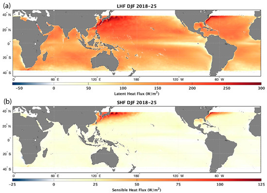
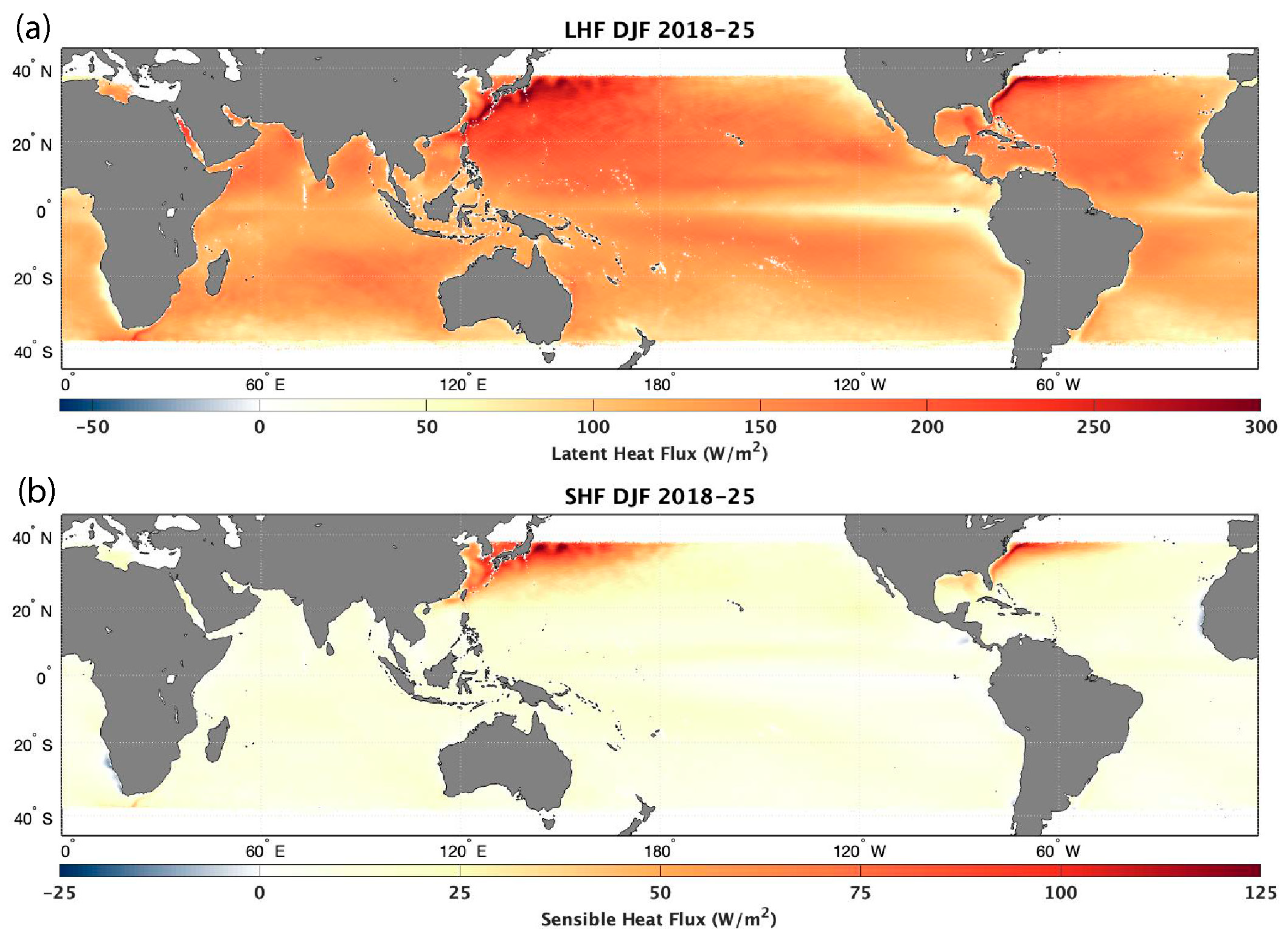
Figure 6 grids the CYGNSS specular points into 0.25° × 0.25° bins and averages them for December, January, and February (DJF, Northern Hemisphere winter) from December 2018 to February 2025 (seven total seasons). In both the LHF (Figure 5a) and SHF (Figure 5b) plots, one can observe the intense surface heat fluxes that are typically observed in the Western Atlantic and Western Pacific Oceans off the East Coasts of the United States and Japan (respectively). This is due to the cold, dry continental air masses interacting with the relatively warm, moist boundary-layer air associated with the Gulf Stream and the Kuroshio Current/Extension. When strong winds are present in these regions (such as during cold-air outbreaks and extratropical cyclogenesis), they amplify LHF and SHF, releasing more moisture and energy from the ocean surface into the marine boundary layer. Additionally, one can observe wave-like patterns in LHF and SHF observations along the Kuroshio Extension (KE), correlating with sea surface temperatures (SSTs) and patterns typically observed in the KE [42]. While DJF is winter in the Northern Hemisphere, it is summer in the Southern Hemisphere, leading to lower LHF and SHF values during this time of year due to minor air–sea thermodynamic differences and the poleward shift in extratropical cyclone tracks. However, the opposite is true for June, July, and August (JJA).
Figure 6.
Average LHF (a) and SHF (b) for the CYGNSS Fluxes for December, January, and February (DJF) from 2018–2025 (seven total seasons).
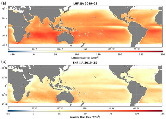
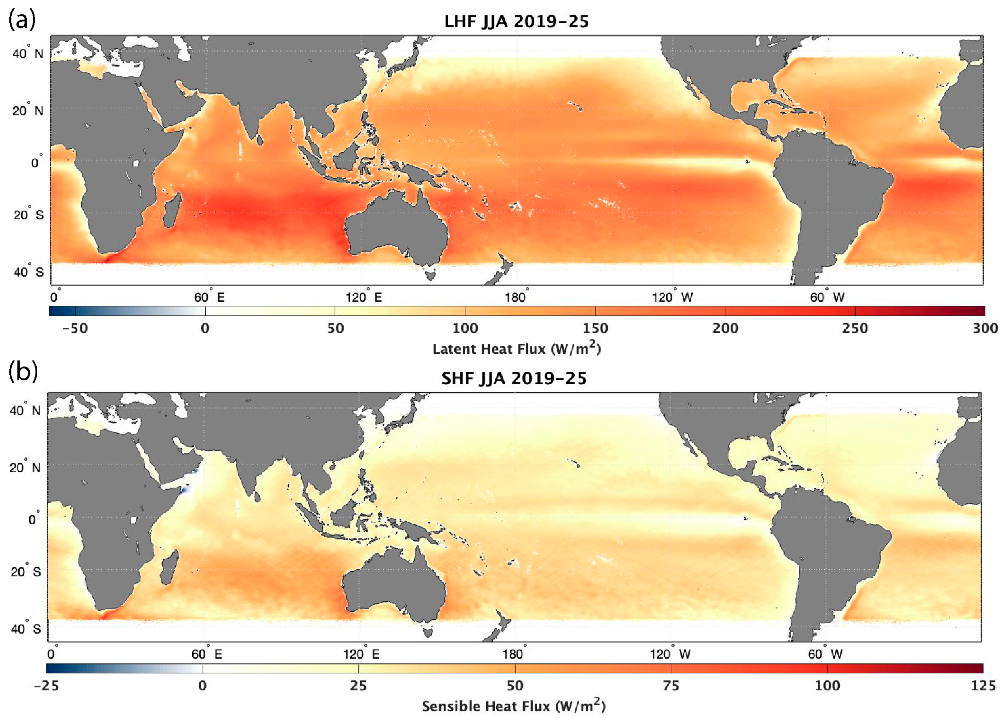
For JJA (Figure 6), this CYGNSS analysis covers the period from 2019 to 2025 (seven complete seasons). While the current CYGNSS dataset began in August 2018, this data was not included in this analysis, as, while its impact on inclusion may be minimal, it would still include an incomplete season. This way, the DJF and JJA results can each include seven complete seasons and be more comparable to each other.
In JJA, both LHF and SHF increase in the Southern Hemisphere during their winter seasons; though not at the same scale as those observed in the Northern Hemisphere winter, the increases in LHF are more evenly distributed than concentrated in specific regions. LHF increases throughout the Southern Indian Ocean, off the coast of South Africa, and in the Southern Equatorial Atlantic Ocean, and on both the western and eastern coasts of Australia. However, for SHF, the only noticeable increases are around South Africa, the Southwest and Southeast coasts of Australia, and off the coast of Uruguay in South America. Additionally, significant negative SHF is observed near Somalia and Yemen around the Gulf of Aden and the western Arabian Sea, while weak (but still positive) LHF is observed. Given that it is summer in these regions, the hot land surface air contributes to negative SHF, while the drier air keeps the LHF positive. In the rest of the Northern Hemisphere, one can see the weakening of the fluxes along the western boundary currents in the Western Pacific and Western Atlantic Oceans; SHF is at or near 0 W/m2 in these regions, while LHF remains slightly elevated in comparison to their surrounding regions, with the differences being slightly larger in and around the Gulf Stream.
While the distribution of LHF and SHF during the DJF and JJA seasons may appear to be common knowledge, Figure 6 and Figure 7 demonstrate CYGNSS’s ability to observe regions of high surface heat fluxes, especially in western boundary currents like the Gulf Stream and KE, despite it being a tropical mission. These plots are similar to previous climatological studies done of LHF and SHF over the oceans [43], indicating that CYGNSS remains a valuable tool for the scientific community in understanding how air–sea interactions impact various meteorological and climatological events.
Figure 7.
Similar to Figure 6, but for June, July, and August (JJA) from 2019—2025 (seven total seasons). (a) LHF in JJA, (b) SHF in JJA.
4.2. Diurnal Results
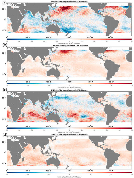
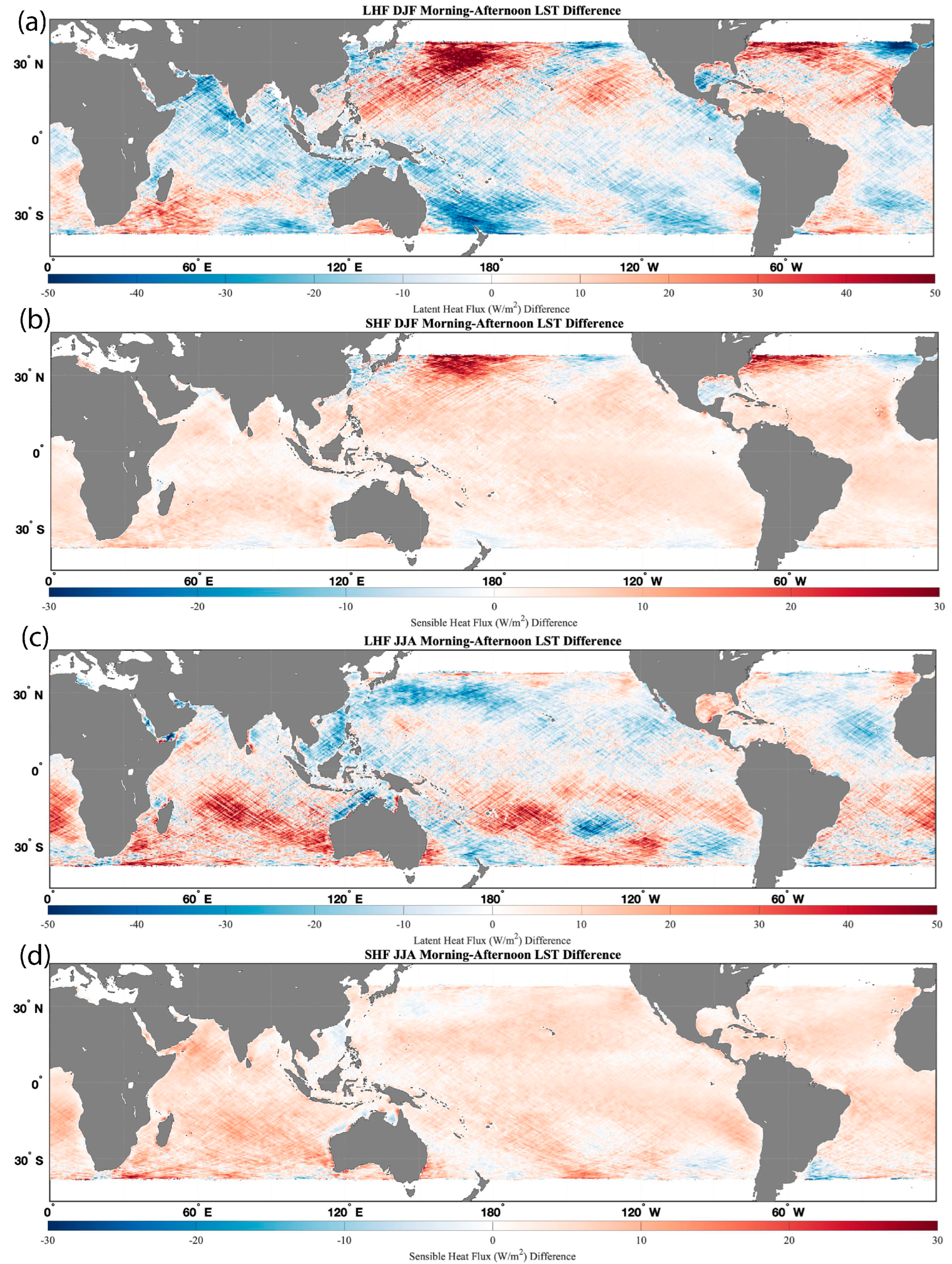
Figure 8 applies the same compositing method of the CYGNSS V3.2 Fluxes, as was shown in Figure 6 and Figure 7, but adds a filter of local solar time (LST) and compares the fluxes between local morning and before sunrise (02:00–05:00 LST) and prior to sunset (14:00–17:00 LST) for each season. Figure 8 illustrates the difference between LHF and SHF in the early morning and afternoon. Plots of the morning and afternoon fluxes for each season, used to estimate the difference, are presented in Supplemental Figures S3–S10.
Figure 8.
Difference in composited CYGNSS Fluxes between local solar time morning (2:00–5:00) and afternoon (14:00–17:00) for (a) LHF during DJF, (b) SHF during DJF, (c) LHF during JJA, and (d) SHF during JJA. Positive values here indicate higher fluxes in the morning than in the afternoon.
For LHF during Northern Hemisphere winter (DJF) (Figure 8a), there is no consistent increase or decrease in fluxes between the early morning and afternoon fluxes, but there are notable differences along the northern edge of CYGNSS’s range, with an increase in LHF in the morning in the Western Atlantic Ocean and most of the Western Pacific Ocean (except near the coast of Japan), and stronger LHF values in the afternoon (negative values) in the Eastern Pacific and Atlantic Oceans. Meanwhile, SHF is typically stronger in the morning across most of the tropical and subtropical oceans, with some exceptions in the Eastern Pacific and Atlantic Oceans near North America and the Iberian Peninsula, as well as south of South Korea (Figure 8b).
Similar patterns emerge during JJA (Southern Hemisphere winter), with SHF being higher in the morning, accompanied by a few pockets of slightly higher afternoon SHF values, such as off the coast of Uruguay and Argentina (Figure 8d). In contrast, the differences are less consistent for LHF (Figure 8c). A wave-like pattern in both LHF difference plots appears to be present, but it is unclear why this is occurring. While we are simply demonstrating the power and utility of CYGNSS’s diurnal observations with its flux product, aided by the inclusion of LST, the authors hope this will motivate future research.
5. Discussion
With nearly a decade of data, CYGNSS provides significant coverage of wind speed and air–sea interaction observations over the tropical and subtropical oceans. As shown in Figure 6 and Figure 7, the data record allows us to composite CYGNSS data over many seasons to better understand the details and changes in LHF and SHF in both hemispheres during their respective winter and summer seasons. While CYGNSS was designed as a tropical mission with an orbit inclination of 35°, its range and field of view are far enough poleward to observe areas of high surface heat fluxes in the winter seasons, such as off the coasts of Japan, the Eastern United States, Australia, Argentina/Uruguay, and South Africa. Many of these areas are common hotspots for extratropical cyclone development, which often have strong surface heat fluxes associated with their genesis and evolution, making CYGNSS an instrumental tool for understanding the impact of air–sea interactions on them [9,10,11].
CYGNSS’s non-sun-synchronous orbit makes it a valuable tool for diurnal analysis at nearly daily timescales in the tropics and seasonal timescales across the whole mission (Figure 1). While diurnal analysis has been performed using CYGNSS data [16,19,44], including local solar time (LST) at every specular point can aid this analysis and enable researchers to produce results similar to those shown in Figure 8. Here, we observe when LHF and SHF are strongest at local time, which can aid in understanding how and when air–sea interactions are likely to impact the genesis and evolution of various weather events.
When comparing the CYGNSS Fluxes to buoy data, one can see that the satellite product compares well with in situ observations at lower flux values, with greater scatter at higher fluxes (Figure 4). We can also observe that in both the tropical and subtropical regions of CYGNSS’s range, the performance of the CYGNSS Fluxes is relatively consistent, even with higher flux values and spread in the subtropical region. Note that the RMSD value obtained in the present analysis is higher than that previously reported in C19. This difference can be partly attributed to the longer temporal span and broader buoy coverage in the matchup dataset used in this study, compared with the shorter period and more limited buoy distribution in the previous validation. Additionally, C19 used buoy data subjected to strict quality control criteria, which excluded coastal observations and consequently limited wind speeds to approximately 11 m/s or less, with little overlap between the data used in C19 and those used in this paper. However, changes to the algorithm, especially when accounting for CYGNSS’s equivalent neutral winds, have reduced biases and errors in areas of instability [35]. A key point is that RMSD values tend to be higher in extratropical regions than in tropical regions (Table 1). This difference is likely due to several factors. First, most extratropical buoys are located closer to the coast, where environmental variability is generally higher. Second, many extratropical coastal buoys tend to have greater measurement uncertainties compared to the TAO buoys commonly deployed in tropical regions; for example, wind measurement errors of around 3% for TAO buoys (https://www.pmel.noaa.gov/gtmba/sensor-specifications, accessed on 4 December 2025) versus approximately 10% for coastal NDBC buoys (https://www.ndbc.noaa.gov/faq/rsa.shtml, accessed on 4 December 2025). Lastly, wind speeds in extratropical areas are typically stronger, increasing the potential for error propagation during the CYGNSS buoy flux validation. Collectively, these factors likely contribute to the elevated RMSD values observed in this study. While the buoy statistics and validation may show similar results, there has nevertheless been an improvement in the uncertainties of the CYGNSS Fluxes, especially at higher flux values (Figure 3). This is primarily due to reduced uncertainty in the CYGNSS wind speed products used for the CYGNSS Fluxes.
Nonetheless, with the more extended dataset, nearly a decade after launch, we have more comparisons than in the initial analysis presented in C19. Despite the significant increase in data and comparisons, we see that CYGNSS Fluxes have gradually improved thanks to the improvements in the wind speed products [20,21], algorithm updates, and the switch from MERRA-2 to ERA5. Additionally, the change from MERRA-2 to ERA5 reduced CYGNSS Flux’s data latency from 1–2 months to 1 week, enabling more immediate analysis of weather and climate events.
Improving the CYGNSS Fluxes beyond this point will depend on improvements to the CYGNSS wind speed products and reanalysis datasets. However, with the mission ending in the coming years, opportunities to improve the dataset using current inputs are limited, despite the desire to improve these surface heat flux estimates. One way to improve CYGNSS Fluxes in the future is to evaluate how they are estimated in the first place. Within the COARE algorithm, wind speed and thermodynamic variables are used to estimate the drag coefficient, which is then used to estimate the friction velocity, which in turn is used to estimate LHF and SHF [33]. While COARE is well tested, the multiple steps required to estimate surface heat fluxes can propagate uncertainties from the input variables, given the nonlinearity in the calculation of the friction velocity. However, it might be possible to estimate friction velocity directly using CYGNSS-observed variables and ancillary data from ERA5. One of the variables CYGNSS directly observes is the mean square slope (MSS), which is closely related to ocean roughness [7]. Since satellites like CYGNSS use ocean roughness to estimate wind speed, MSS observations from CYGNSS can be more accurate, as they are nearly a direct observation. While there is no direct way to estimate friction velocity (and therefore surface heat fluxes) from MSS, machine learning could be used to understand the relationship between MSS, Leading Edge Slope (LES), and other directly observed CYGNSS observations, along with ancillary data from reanalysis, to directly estimate friction velocity. This machine learning method could be trained using in situ observations from buoys and field campaigns to better refine these estimates. This would also simplify the algorithms used to estimate surface heat fluxes, as the friction velocity would be provided directly rather than estimated separately. More work is needed to refine this approach, but we believe it can greatly improve surface heat flux estimates and serve as a model for future missions.
6. Conclusions
Since its launch, CYGNSS has been an invaluable tool for analyzing wind speed and air–sea interactions over tropical and subtropical oceans. While the mission’s future is uncertain, the CYGNSS Fluxes have been a valuable tool since their initial development [8], and we hope they continue to be used after CYGNSS is retired. Since its initial release, the CYGNSS Fluxes have incorporated updates to the CYGNSS L2 wind speed products, shifted from MERRA-2 to ERA5 for thermodynamic inputs, and slightly updated the COARE 3.5 algorithm to account for equivalent neutral winds produced by CYGNSS. These changes have led to improvements in the CYGNSS Fluxes and reduced data latency, allowing scientists and researchers to use the data more frequently. While in situ data remain the preferred source for air–sea interactions, our results here and in the past show that CYGNSS is a valuable tool when in situ data are unavailable, and its data complement other satellite missions focused on providing surface and marine boundary layer observations. The latest CYGNSS Ocean Surface Heat Flux Product is available through NASA’s Physical Oceanography Distributed Active Archive Center (PO.DAAC), with data ranging from 1 August 2018 through the present, with a time lag of about 1 week.
The projected timeline for CYGNSS’s observations is scheduled to end in October 2026, when support for the mission is also slated to end. While this date may change, the plan is to continue providing LHF and SHF observations using CYGNSS data through the end of its mission. While CYGNSS itself may be sunsetting, various GNSS-R missions have been launched through the public and private sectors, such as HydroGNSS [45] and MuSat2 [46]. While these missions are aimed at improving observations of soil moisture and inland water, which CYGNSS has also excelled at [47], they could also be used to estimate LHF and SHF over the oceans, complementing overlapping CYGNSS observations and providing key observations after CYGNSS’s retirement.
The CYGNSS Fluxes show the need for continued improvement of observations of air–sea interactions from space. While CYGNSS is a valuable tool, it is limited to observing wind speeds over the ocean, so temperature and humidity must come from other sources. In CYGNSS’s case, this is done using reanalysis data due to their availability and minimal time differences relative to the CYGNSS specular point observations. However, these datasets still contain limitations and biases that affect the CYGNSS Fluxes, making the flux product less independent. At the time of writing, there are no active satellite missions that can estimate LHF and SHF using onboard instruments; however, missions are being proposed that would provide these kinds of observations, such as Butterfly [48]. Our goal is that the results from the CYGNSS mission will provide additional justification for these missions; improving spaceborne observations of air–sea interactions and the marine boundary layer is a critical need for NASA and other space agencies worldwide. As stated in the 2017 Decadal Survey: “Coincident estimates of surface fluxes at higher spatial resolution and accuracy than currently available from satellite…would provide crucial improvements needed to address the understanding of the impacts of the ocean mesoscale” [49].
Supplementary Materials
The following supporting information can be downloaded at: https://www.mdpi.com/article/10.3390/rs18091353/s1, Figure S1: The Equation of Time (EoT) adjustment in seconds as a function of the day of the year 13 (DoY); estimated from Equations 1 and 2; Figure S2: The uncertainty (sigma) of LHF (a) and SHF (b) at every specular point using a pertur-bation/uncertainty method as described in C19. Rather than repeat this process for every specular point for the CYGNSS Fluxes, a best-fit line was used to estimate uncertainty (sigma) as a function of LHF and SHF (black lines). In the latest versions of the CYGNSS Fluxes, a logarithmic best-fit function was used in order to better capture the uncertainty for LHF below 100 W m-2 and SHF be-low 25 W m-2 (blue). These equations were then used to show the uncertainties plotted in Figure 5. Given a similar, but mirrored, distribution of uncertainties for negative fluxes (not shown here), the equations were mirrored for negative values; Figure S3: Average Latent Heat Flux (LHF) from December, January, and February (DJF) across seven seasons (2018-2025) when the local solar time (LST) is between 2–5 am; Figure S4: Same as S3, but for LST between 2–5 pm (14:00–17:00); Figure S5: Same as S3, but for Sensible Heat Flux (SHF); Figure S6: Same as S5, but for LST between 2–5 pm (14:00–17:00); Figure S7: Same as S3, but for June, July, and August (JJA) across seven seasons (2019–2025); Figure S8: Same as S7, but for LST between 2–5 pm (14:00–17:00); Figure S9: Same as S7, but for Sensible Heat Flux (SHF); Figure S10: Same as S9, but for LST between 2–5 pm (14:00–17:00).
Author Contributions
J.A.C. has led the development of the CYGNSS Fluxes and wrote a majority of this paper, as well as creating Figure 1, Figure 2, Figure 5, Figure 6 and Figure 7. S.A. led the buoy validation, created Figure 3 and Figure 4, and contributed to the analysis in those sections. A.R. and D.T. contributed to the discussion on the tri-linear interpolation, implemented the local solar time estimates, and helped finalize the CYGNSS Fluxes at CYGNSS’s Science Operations Center (SOC) before the product was published through the PO.DAAC. D.J.P. helped with the initial versions of the CYGNSS fluxes and contributed to various portions of the paper. All authors have read and agreed to the published version of the manuscript.
Funding
This research was funded by the CYGNSS mission under NASA Science Mission Directorate Contract NNL13AQ00C and by JPL Subcontracts 1669120 and 1658425.
Data Availability Statement
The latest CYGNSS Ocean Surface Heat Flux Product (SDR V3.2) used for this paper is available through NASA’s Physical Oceanography Distributed Active Archive Center (PO.DAAC), with data ranging from 1 August 2018 through the present, with a time lag of about 1 week at this link: https://podaac.jpl.nasa.gov/dataset/CYGNSS_L2_SURFACE_FLUX_V3.2 (accessed on 10 September 2025). Buoy data used for the comparison and validation section can be found through NOAA’s NDBC database: https://www.ndbc.noaa.gov/historical_data.shtml (accessed on 28 September 2025).
Acknowledgments
We would like to thank Mary Morris at the NASA Jet Propulsion Laboratory (JPL) for her assistance with compositing the CYGNSS Fluxes and for providing feedback on this paper. We would also like to thank past and present members of the Physical Oceanography Distributed Active Archive Center (PO.DAAC) at JPL, especially David Moroni and Yibo Jiang, for their assistance in developing the CYGNSS Surface Heat Flux Product and releasing it to the public. Finally, we would like to thank Christopher Ruf, the PI of the CYGNSS mission, for his assistance and support in developing and maintaining the CYGNSS Ocean Surface Heat Flux product. Part of this work was carried out at the Jet Propulsion Laboratory, California Institute of Technology, under a contract with the National Aeronautics and Space Administration. Copyright 2026 California Institute of Technology. Government sponsorship acknowledged.
Conflicts of Interest
The authors declare no conflicts of interest.
Abbreviations
The following abbreviations are used in this manuscript:
| C19 | Crespo et al. 2019 [8] |
| CDR | Climate Data Record |
| COARE | Coupled Ocean–Atmosphere Response Experiment |
| CYGNSS | Cyclone Global Navigation Satellite System |
| DDM | Delay Doppler Map |
| DDMA | DDM Average |
| DJF | December, January, and February |
| ECMWF | European Centre for Medium-Range Weather Forecasts |
| EoT | Equation of Time |
| ERA5 | ECMWF Reanalysis, Version 5 |
| ET | Extratropics |
| ETC | Extratropical Cyclone |
| FDS | Fully Developed Seas |
| GNSS-R | Global Navigation Satellite System-Reflectometry |
| GPS | Global Positioning System |
| JJA | June, July, and August |
| KE | Kuroshio Extension |
| KEO | Kuroshio Extension Observatory |
| L1 | Level 1 |
| L2 | Level 2 |
| L3 | Level 3 |
| LES | Leading-Edge Slope |
| LHF | Latent Heat Flux |
| LST | Local Solar Time |
| MBL | Marine Boundary Layer |
| MERRA-2 | Modern-Era Retrospective Analysis for Research and Applications, Version 2 |
| MSS | Mean Square Slope |
| NASA | National Aeronautics and Space Administration |
| NDBC | National Data Buoy Center |
| NOAA | National Oceanic and Atmospheric Administration |
| PIRATA | Prediction and Research Moored Array in the Tropical Atlantic |
| PO.DAAC | Physical Oceanography Distributed Active Archive Center |
| RMSD | Root Mean Square Difference |
| SOC | Science Operations Center |
| SDR | Science Data Record |
| SHF | Sensible Heat Flux |
| SST | Sea Surface Temperature |
| TAO | Tropical Atmosphere Ocean Array |
| TC | Time Correction |
| UTC | Universal Coordinated Time |
| YSLF | Young Seas with Limited Fetch |
References
- Emanuel, K.A. An Air-Sea Interaction Theory for Tropical Cyclones. Part I: Steady-State Maintenance. J. Atmos. Sci. 1986, 43, 585–605. [Google Scholar] [CrossRef] [Scilit]
- Neiman, P.J.; Shapiro, M.A. The Life Cycle of an Extratropical Marine Cyclone. Part I: Frontal-Cyclone Evolution and Thermodynamic Air-Sea Interaction. Mon. Weather Rev. 1993, 121, 2153–2176. [Google Scholar] [CrossRef] [Scilit]
- Sun, R.; Subramanian, A.C.; Cornuelle, B.D.; Mazloff, M.R.; Miller, A.J.; Ralph, F.M.; Seo, H.; Hoteit, I. The Role of Air–Sea Interactions in Atmospheric Rivers: Case Studies Using the SKRIPS Regional Coupled Model. J. Geophys. Res. Atmos. 2021, 126, e2020JD032885. [Google Scholar] [CrossRef] [Scilit]
- Jones, C.; Weare, B.C. The Role of Low-Level Moisture Convergence and Ocean Latent Heat Fluxes in the Madden and Julian Oscillation: An Observational Analysis Using ISCCP Data and ECMWF Analyses. J. Clim. 1996, 9, 3086–3104. [Google Scholar] [CrossRef] [Scilit]
- Liu, W.T.; Katsaros, K.B.; Businger, J.A. Bulk Parameterization of Air-Sea Exchanges of Heat and Water Vapor Including the Molecular Constraints at the Interface. J. Atmos. Sci. 1979, 36, 1722–1735. [Google Scholar] [CrossRef] [Scilit]
- Ruf, C.S.; Atlas, R.; Chang, P.S.; Clarizia, M.P.; Garrison, J.L.; Gleason, S.; Katzberg, S.J.; Jelenak, Z.; Johnson, J.T.; Majumdar, S.J.; et al. New Ocean Winds Satellite Mission to Probe Hurricanes and Tropical Convection. Bull. Am. Meteorol. Soc. 2016, 97, 385–395. [Google Scholar] [CrossRef] [Scilit]
- Ruf, C. CYGNSS Handbook 2022, 2nd ed.; Michigan Publishing Services: Ann Arbor, MI, USA, 2022. [Google Scholar]
- Crespo, J.; Posselt, D.; Asharaf, S. CYGNSS Surface Heat Flux Product Development. Remote Sens. 2019, 11, 2294. [Google Scholar] [CrossRef] [Scilit]
- Crespo, J.A.; Naud, C.M.; Posselt, D.J. CYGNSS Observations and Analysis of Low-Latitude Extratropical Cyclones. J. Appl. Meteorol. Climatol. 2021, 60, 527–541. [Google Scholar] [CrossRef] [Scilit]
- Naud, C.M.; Crespo, J.A.; Posselt, D.J. On the Relationship between CYGNSS Surface Heat Fluxes and the Lifecycle of Low-Latitude Ocean Extratropical Cyclones. J. Appl. Meteorol. Climatol. 2021, 60, 1575–1590. [Google Scholar] [CrossRef] [Scilit]
- Naud, C.M.; Crespo, J.A.; Posselt, D.J.; Booth, J.F. Cloud and Precipitation in Low-Latitude Extratropical Cyclones Conditionally Sorted on CYGNSS Surface Latent and Sensible Heat Fluxes. J. Clim. 2023, 36, 5659–5680. [Google Scholar] [CrossRef] [Scilit]
- LeGrande, A.N.; Booth, J.F.; Naud, C.M.; Ordaz, C.; Crespo, J.A. Just How River-Like Are Atmospheric Rivers? Geophys. Res. Lett. 2024, 51, e2023GL105828. [Google Scholar] [CrossRef] [Scilit]
- Asharaf, S.; Guan, B.; Waliser, D.E. CYGNSS Satellite Sampling of Surface Heat Fluxes Across Atmospheric River Life Cycles. Geophys. Res. Lett. 2025, 52, e2024GL113370. [Google Scholar] [CrossRef] [Scilit]
- Aiyyer, A.; Schreck, C. Surface Wind Speeds and Enthalpy Fluxes During Tropical Cyclone Formation From Easterly Waves: A CYGNSS View. Geophys. Res. Lett. 2023, 50, e2022GL100823. [Google Scholar] [CrossRef] [Scilit]
- Bui, H.X.; Maloney, E.D.; Riley Dellaripa, E.M.; Singh, B. Wind Speed, Surface Flux, and Intraseasonal Convection Coupling From CYGNSS Data. Geophys. Res. Lett. 2020, 47, e2020GL090376. [Google Scholar] [CrossRef] [Scilit]
- Riley Dellaripa, E.M.; Maloney, E.D.; DeMott, C.A. The Diurnal Cycle of East Pacific Convection, Moisture, and CYGNSS Wind Speed and Fluxes. J. Geophys. Res. Atmos. 2023, 128, e2022JD038133. [Google Scholar] [CrossRef] [Scilit]
- Hudson, J.; Maloney, E. The Role of Surface Fluxes in MJO Propagation through the Maritime Continent. J. Clim. 2023, 36, 1633–1652. [Google Scholar] [CrossRef] [Scilit]
- Li, X.; Yang, J.; Yan, Y.; Li, W. Exploring CYGNSS Mission for Surface Heat Flux Estimates and Analysis over Tropical Oceans. Front. Mar. Sci. 2022, 9, 1001491. [Google Scholar] [CrossRef] [Scilit]
- Lin, J.; Wang, Y.; Pan, H.; Wei, Z.; Xu, T. Uncertainty of CYGNSS-Derived Heat Flux Variations at Diurnal to Seasonal Time Scales over the Tropical Oceans. Remote Sens. 2023, 15, 3161. [Google Scholar] [CrossRef] [Scilit]
- Ruf, C.; Al-Khaldi, M.; Asharaf, S.; Balasubramaniam, R.; McKague, D.; Pascual, D.; Russel, A.; Twigg, D.; Warnock, A. Characterization of CYGNSS Ocean Surface Wind Speed Products. Remote Sens. 2024, 16, 4341. [Google Scholar] [CrossRef] [Scilit]
- Asharaf, S.; Waliser, D.E.; Posselt, D.J.; Ruf, C.S.; Zhang, C.; Putra, A.W. CYGNSS Ocean Surface Wind Validation in the Tropics. J. Atmos. Ocean. Technol. 2021, 38, 711–724. [Google Scholar] [CrossRef] [Scilit]
- Asharaf, S.; Posselt, D.J.; Said, F.; Ruf, C.S. Updates on CYGNSS Ocean Surface Wind Validation in the Tropics. J. Atmos. Ocean. Technol. 2023, 40, 37–51. [Google Scholar] [CrossRef] [Scilit]
- Warnock, A.M.; Ruf, C.S.; Russel, A.; Al-Khaldi, M.M.; Balasubramaniam, R. CYGNSS Level 3 Merged Wind Speed Data Product for Storm Force and Surrounding Environmental Winds. IEEE J. Sel. Top. Appl. Earth Obs. Remote Sens. 2024, 17, 6189–6200. [Google Scholar] [CrossRef] [Scilit]
- Said, F.; Jelenak, Z.; Park, J.; Chang, P.S. The NOAA Track-Wise Wind Retrieval Algorithm and Product Assessment for CyGNSS. IEEE Trans. Geosci. Remote Sens. 2022, 60, 1–24. [Google Scholar] [CrossRef] [Scilit]
- CYGNSS. CYGNSS Level 2 Science Data Record, Version 3.2; NASA: Pasadena, CA, USA, 2024.
- CYGNSS. CYGNSS Level 2 Ocean Surface Heat Flux Science Data Record, Version 3.2; NASA: Pasadena, CA, USA, 2024.
- Gelaro, R.; McCarty, W.; Suárez, M.J.; Todling, R.; Molod, A.; Takacs, L.; Randles, C.A.; Darmenov, A.; Bosilovich, M.G.; Reichle, R.; et al. The Modern-Era Retrospective Analysis for Research and Applications, Version 2 (MERRA-2). J. Clim. 2017, 30, 5419–5454. [Google Scholar] [CrossRef] [Scilit]
- CYGNSS. CYGNSS Level 2 Climate Data Record, Version 1.1; NASA: Pasadena, CA, USA, 2020.
- Hersbach, H.; Bell, B.; Berrisford, P.; Hirahara, S.; Horányi, A.; Muñoz-Sabater, J.; Nicolas, J.; Peubey, C.; Radu, R.; Schepers, D.; et al. The ERA5 Global Reanalysis. Q. J. R. Meteorol. Soc. 2020, 146, 1999–2049. [Google Scholar] [CrossRef] [Scilit]
- Serra, Y.L.; Rutledge, S.A.; Chudler, K.; Zhang, C. Rainfall and Convection in ERA5 and MERRA-2 over the Northern Equatorial Western Pacific during PISTON. J. Clim. 2023, 36, 845–863. [Google Scholar] [CrossRef] [Scilit]
- Tulger Kara, G.; Elbir, T. Seasonal and Spatial Variability in the Accuracy of Hourly ERA5 and MERRA-2 Reanalysis Datasets: A 14-Year Comparison with Observed Meteorological Data in Türkiye. Atmos. Res. 2025, 325, 108233. [Google Scholar] [CrossRef] [Scilit]
- Huang, L.; Fang, X.; Zhang, T.; Wang, H.; Cui, L.; Liu, L. Evaluation of Surface Temperature and Pressure Derived from MERRA-2 and ERA5 Reanalysis Datasets and Their Applications in Hourly GNSS Precipitable Water Vapor Retrieval over China. Geod. Geodyn. 2023, 14, 111–120. [Google Scholar] [CrossRef] [Scilit]
- Edson, J.B.; Jampana, V.; Weller, R.A.; Bigorre, S.P.; Plueddemann, A.J.; Fairall, C.W.; Miller, S.D.; Mahrt, L.; Vickers, D.; Hersbach, H. On the Exchange of Momentum over the Open Ocean. J. Phys. Oceanogr. 2013, 43, 1589–1610. [Google Scholar] [CrossRef] [Scilit]
- Bourassa, M.A.; Hughes, P.J. Turbulent Heat Fluxes and Wind Remote Sensing. In New Frontiers in Operational Oceanography; Chassignet, E.P., Pascual, A., Tintoré, J., Verron, J., Eds.; GODAE OceanView: Exeter, UK, 2018. [Google Scholar]
- Asharaf, S.; Crespo, J.A.; Posselt, D.J.; Bourassa, M.A. Advancing CYGNSS-Derived Ocean Surface Heat Fluxes. Remote Sens. 2026, 18, 694. [Google Scholar] [CrossRef] [Scilit]
- Rees, W.G. Calculating the Parameters of the Earth’s Orbit. Eur. J. Phys. 1991, 12, 96–100. [Google Scholar] [CrossRef] [Scilit]
- Park, J.; Johnson, J.T.; Yi, Y.; O’Brien, A.J. Using “Rapid Revisit” CYGNSS Wind Speed Measurements to Detect Convective Activity. IEEE J. Sel. Top. Appl. Earth Obs. Remote Sens. 2019, 12, 98–106. [Google Scholar] [CrossRef] [Scilit]
- Hamilton, G.D. National Data Buoy Center Programs. Bull. Am. Meteorol. Soc. 1986, 67, 411–415. [Google Scholar] [CrossRef] [Scilit]
- McPhaden, M.J.; Busalacchi, A.J.; Cheney, R.; Donguy, J.; Gage, K.S.; Halpern, D.; Ji, M.; Julian, P.; Meyers, G.; Mitchum, G.T.; et al. The Tropical Ocean-Global Atmosphere Observing System: A Decade of Progress. J. Geophys. Res. 1998, 103, 14169–14240. [Google Scholar] [CrossRef] [Scilit]
- Bourlès, B.; Lumpkin, R.; McPhaden, M.J.; Hernandez, F.; Nobre, P.; Campos, E.; Yu, L.; Planton, S.; Busalacchi, A.; Moura, A.D.; et al. THE PIRATA PROGRAM: History, Accomplishments, and Future Directions. Bull. Am. Meteorol. Soc. 2008, 89, 1111–1126. [Google Scholar] [CrossRef] [Scilit]
- Cronin, M.F.; Meinig, C.; Sabine, C.L.; Ichikawa, H.; Tomita, H. Surface mooring network in the Kuroshio Extension. IEEE Syst. J. 2008, 2, 424–430. [Google Scholar] [CrossRef] [Scilit]
- Qiu, B. Interannual Variability of the Kuroshio Extension System and Its Impact on the Wintertime SST Field. J. Phys. Oceanogr. 2000, 30, 1486–1502. [Google Scholar] [CrossRef] [Scilit]
- Yu, L.S.; Weller, R.A. Objectively analyzed air-sea heat fluxes for the global ice-free oceans (1981–2005). Bull. Am. Meteorol. Soc. 2007, 88, 527–539. [Google Scholar] [CrossRef] [Scilit]
- Yi, Y.; Johnson, J.T.; Wang, X. Diurnal Variations in Ocean Wind Speeds Measured by CYGNSS and Other Satellites. IEEE Geosci. Remote Sens. Lett. 2022, 19, 1–5. [Google Scholar] [CrossRef] [Scilit]
- Unwin, M.J.; Pierdicca, N.; Cardellach, E.; Rautiainen, K.; Foti, G.; Blunt, P.; Guerriero, L.; Santi, E.; Tossaint, M. An Introduction to the HydroGNSS GNSS Reflectometry Remote Sensing Mission. IEEE J. Sel. Top. Appl. Earth Obs. Remote Sens. 2021, 14, 6987–6999. [Google Scholar] [CrossRef] [Scilit]
- Roberts, M.; Colwell, I.; Chew, C.; Masters, D.; Nordstrom, K. The Muon Space GNSS-R Surface Soil Moisture Product. arXiv 2024, arXiv:2412.00072. [Google Scholar]
- Clarizia, M.P.; Pierdicca, N.; Costantini, F.; Floury, N. Analysis of CYGNSS Data for Soil Moisture Retrieval. IEEE J. Sel. Top. Appl. Earth Obs. Remote Sens. 2019, 12, 2227–2235. [Google Scholar] [CrossRef] [Scilit]
- Gentemann, C.L.; Clayson, C.A.; Brown, S.; Lee, T.; Parfitt, R.; Farrar, J.T.; Bourassa, M.; Minnett, P.J.; Seo, H.; Gille, S.T.; et al. FluxSat: Measuring the Ocean–Atmosphere Turbulent Exchange of Heat and Moisture from Space. Remote Sens. 2020, 12, 1796. [Google Scholar] [CrossRef] [Scilit]
- Teixeira, J.; Piepmeier, J.R.; Nehrir, A.R.; Ao, C.O.; Chen, S.S.; Clayson, C.A.; Fridlind, A.M.; Lebsock, M.; McCarty, W.; Salmun, H.; et al. Toward a Global Planetary Boundary Layer Observing System: The NASA PBL Incubation Study Team Report; NASA PBL Incubation Study Team: Pasadena, CA, USA, 2021; 134p.

Disclaimer/Publisher’s Note: The statements, opinions and data contained in all publications are solely those of the individual author(s) and contributor(s) and not of MDPI and/or the editor(s). MDPI and/or the editor(s) disclaim responsibility for any injury to people or property resulting from any ideas, methods, instructions or products referred to in the content. |
© 2026 by the authors. Licensee MDPI, Basel, Switzerland. This article is an open access article distributed under the terms and conditions of the Creative Commons Attribution (CC BY) license.