MultTransNet: A Novel Multimodal Transformer Network for Retrieving Significant Wave Height Using GNSS-R Data

Highlights

What are the main findings?

• The proposed MultTransNet effectively fuses 2D Delay–Doppler Map (DDM) images with 1D auxiliary parameters, reducing Root Mean Square Error (RMSE) by 27.05% and increasing the correlation coefficient (CC) by 7.21% compared with single-modality models.
• An XGBoost-based iterative feature selection method optimizes the input predictors from 20 to 11 key variables, significantly improving the accuracy of significant wave height (SWH) retrieval, particularly under complex sea-state conditions.

What are the implications of the main findings?

• The fusion of spatial image features and numerical parameters overcomes the limitations of single-modality GNSS-R observations and enhances model robustness in complex marine environments.
• The improved accuracy and global consistency of the proposed approach enable more reliable all-weather SWH retrieval, supporting marine forecasting, maritime safety, and disaster mitigation.

Abstract

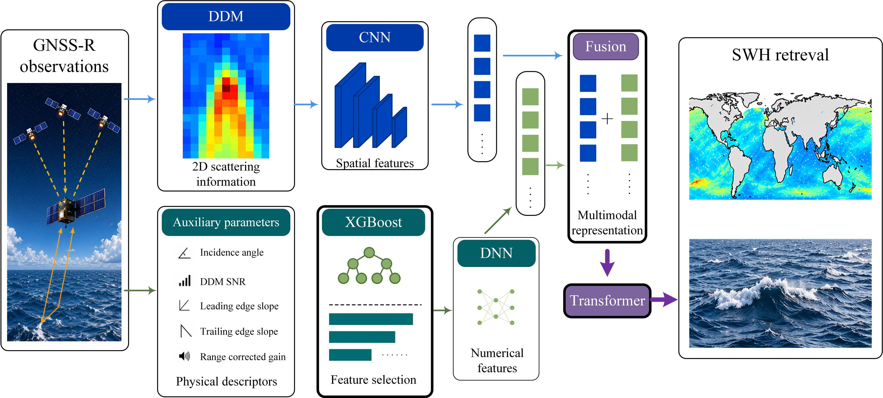
Significant Wave Height (SWH) is a critical parameter for ocean observation. SWH retrieval using GNSS-R data faces challenges including difficult feature selection, insufficient temporal dependency modeling, and limitations due to single-modality data. This paper proposes a novel Multimodal Transformer Network (MultTransNet) to enhance the accuracy of GNSS-R SWH retrieval. To optimize the feature set, we designed an XGBoost-based iterative feature selection module that effectively eliminates redundant features. To capture complex temporal dependencies and global context, the model employs a Transformer encoder utilizing its self-attention mechanism. Furthermore, to overcome the constraints of single-modality data, we innovatively fused 2D DDM image data with 1D auxiliary parameters, enabling multi-source information integration. Simulation results show that the Transformer architecture reduces Root Mean Square Error (RMSE) by 8.91% and increases Correlation Coefficient (CC) by 4.05% compared to a conventional Deep Neural Network (DNN) model. More significantly, the proposed multimodal algorithm further improves retrieval accuracy by 27.05% (RMSE reduction) and 7.21% (CC increase) compared to its single-modality Transformer counterpart, demonstrating superior performance, especially in complex sea-state conditions.

1. Introduction

Significant Wave Height (SWH), defined as the mean height of the highest one-third of waves in a continuous sequence, is a fundamental physical parameter in oceanography and maritime operations [1]. It provides an intuitive representation of wave energy distribution and plays a pivotal role in marine meteorological forecasting, maritime safety, and coastal engineering [2,3]. Analyzing SWH variations prior to extreme weather events, such as typhoons, provides crucial support for coastal regions in formulating scientific disaster mitigation strategies, thereby effectively reducing economic losses [4].

Consequently, the efficient acquisition of continuous, large-scale, and high-precision SWH data remains a persistent objective in oceanographic observation [5].

Traditional ocean wave monitoring predominantly relies on in situ buoys, satellite altimetry, and Synthetic Aperture Radar (SAR) [6]. While buoys offer highly accurate direct measurements, their sparse spatial distribution and prohibitive deployment costs hinder continuous global monitoring [6]. Satellite altimeters are suitable for large-scale observations but are constrained by narrow swath widths and low temporal resolution [7,8]. Although SAR technology achieves high spatial resolution, its data processing is computationally intensive, and its retrieval accuracy is highly sensitive to specific extreme sea states [9,10]. To circumvent these limitations, spaceborne Global Navigation Satellite System-Reflectometry (GNSS-R) has emerged as an innovative remote sensing paradigm. By opportunistically utilizing signals from navigation satellite constellations, spaceborne GNSS-R offers unprecedented advantages, including cost-effectiveness, high spatiotemporal resolution, and all-weather observation capabilities capable of penetrating heavy precipitation [11,12,13].

In recent years, the research paradigm for SWH retrieval using spaceborne GNSS-R has experienced a profound transition from shallow machine learning to deep feature mining and global modeling. Early machine learning approaches, such as Support Vector Machines (SVM) [14] and ensemble tree models [15], demonstrated superior performance over traditional empirical models when handling multi-variable inputs. However, these methods were predominantly confined to 1D scalar observables, failing to exploit the rich spatial structural information inherent in Delay–Doppler Maps (DDMs). To overcome this bottleneck, researchers introduced Deep Convolutional Neural Networks (DCNNs) to directly extract the spatial texture of scattering energy from 2D DDM images, achieving significant improvements in retrieval accuracy [16].

Nevertheless, as research progressed, the inherent limitations of Convolutional Neural Networks (CNNs) regarding their restricted receptive fields became apparent [17], rendering them insufficient for establishing long-range dependencies across the entire DDM. Consequently, the most recent cutting-edge studies have begun exploring Transformer architectures within the GNSS-R domain. For instance, newly developed models such as WaveFormer have successfully leveraged self-attention mechanisms to capture both local and global spatial features, comprehensively outperforming traditional CNN-based methods [18]. Furthermore, to address the critical challenge of sharp error increases under extreme sea states (e.g., tropical cyclones), recent studies emphasize the necessity of employing advanced algorithms like XGBoost for feature reconstruction and prior optimization to mitigate the high-dimensional information redundancy and non-linear perturbations caused by complex marine environments [19]. These state-of-the-art explorations strongly indicate that the integration of efficient feature selection mechanisms with multimodal deep learning architectures possessing global perception capabilities has become the pivotal key to achieving high-precision SWH retrieval under complex sea states.

To overcome this bottleneck, machine learning algorithms equipped with robust high-dimensional data processing capabilities have progressively emerged as the mainstream approach. From Support Vector Machines (SVM) [14] to ensemble tree models like Random Forest (RF) and XGBoost [15], shallow machine learning has demonstrated significantly superior performance over traditional models when handling multi-variable inputs. With the explosive growth of satellite data, Deep Learning architectures, such as Deep Neural Networks (DNNs) [20], have further elevated the upper bounds of retrieval accuracy. Most recently, cutting-edge studies have conducted comprehensive comparative analyses across various advanced deep learning and ensemble tree models, firmly establishing the dominant superiority of deep learning architectures in processing complex, multi-variable GNSS-R observations [21]. Concurrently, these studies underscore that as the dimensionality of available environmental parameters surges, models are highly susceptible to information redundancy, necessitating more efficient and advanced feature optimization strategies.

Despite these advancements, current machine learning-based GNSS-R SWH retrieval methods still face three critical challenges:

• Limitations in Feature Selection: Current feature selection predominantly relies on empirical manual screening [22,23], which struggles to comprehensively evaluate deep inter-feature correlations. This often results in information redundancy or the inadvertent omission of key physical predictors.
• Inadequate Temporal Modeling: Existing time-series modeling approaches exhibit inherent bottlenecks in extracting long-range temporal dependencies [20], failing to adequately characterize the complex spatiotemporal evolution of sea state features along the satellite ground tracks.
• Constraints of Single-Modality Data: The vast majority of current studies depend exclusively on 1D scalar observables [23], discarding the rich 2D spatial texture and scattering energy distribution information inherent in the original DDMs. This single-modality constraint severely limits the model’s robustness and comprehensive performance, particularly under complex or extreme high sea-state conditions.

To address these fundamental challenges, this paper proposes a novel GNSS-R SWH retrieval model based on a Multimodal Transformer Network (MultTransNet). The primary contributions of this study are systematically outlined as follows:

• Feature Optimization: We designed an XGBoost-based iterative feature selection module that comprehensively evaluates both feature importance and Pearson correlation. This approach effectively eliminates redundant variables while retaining the most critical physical predictors contributing to SWH.
• Temporal Enhancement: By introducing a Transformer encoder architecture, the model leverages multi-head self-attention mechanisms to capture global contextual information within the satellite observation sequence, effectively overcoming the short-term memory limitations of traditional sequence models.
• Multimodal Fusion: We innovatively fused 2D DDM spatial image features (extracted via CNN) with 1D optimized auxiliary parameters (processed via DNN). This integration of multi-source information significantly enhances the retrieval accuracy and physical interpretability of the model under complex marine environments.

2. Methodology

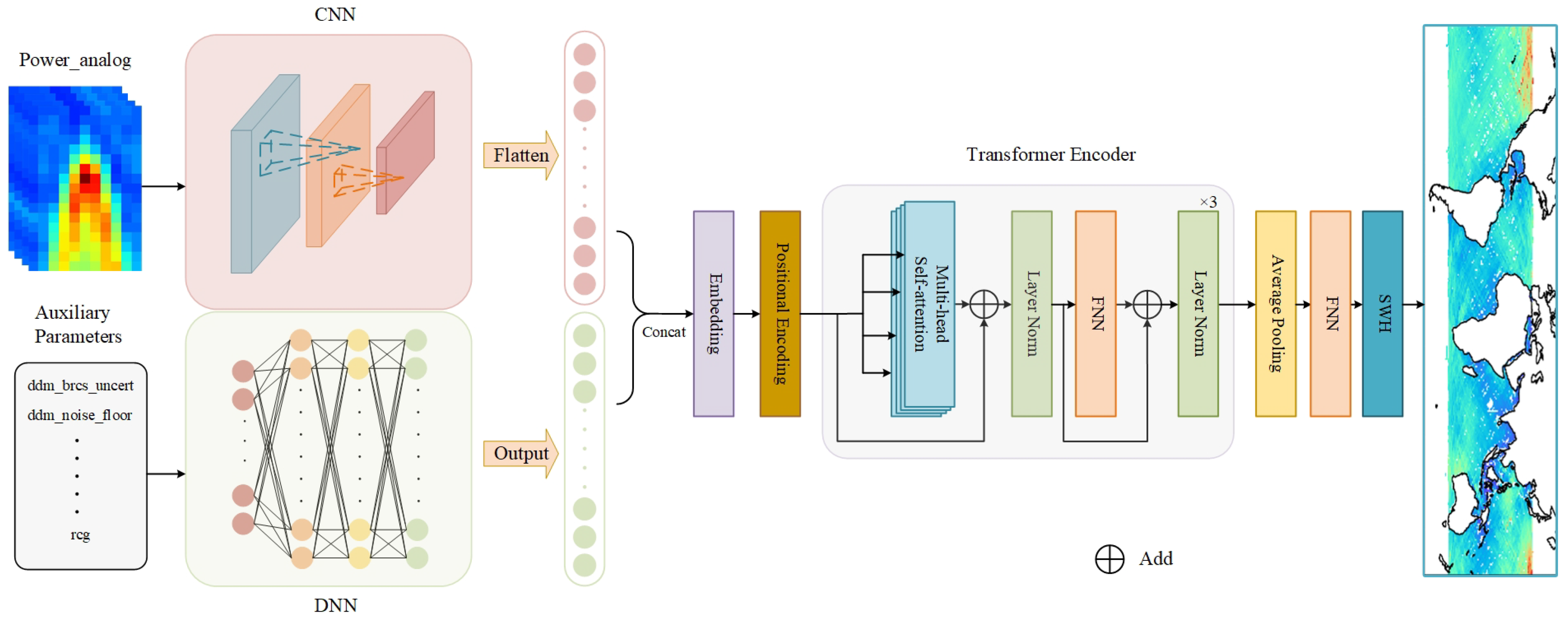
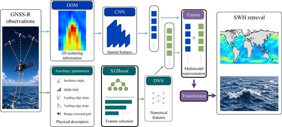
This section details the architecture of the proposed MultTransNet model. As illustrated in Figure 1, MultTransNet comprises four key components.

2.1. DNN-Based Feature Extractor

The DNN feature extractor processes a 1D vector of GNSS-R parameters, which represents the optimal feature subset identified by the XGBoost algorithm (detailed in Section 3). Its primary function is to capture the deep, non-linear relationships inherent in these inputs. The architecture is a multi-layer perceptron (MLP) consisting of several fully connected layers, each followed by a non-linear activation function. This hierarchical design enables the model to progressively learn a cascade of increasingly abstract feature representations, effectively mining the intricate interdependencies among the key observables. The module’s output is a dense, information-rich feature vector that serves as a powerful, representative input for the subsequent Transformer encoder, thereby providing a robust foundation for the final SWH retrieval. In the final model configuration, this branch takes the 11 optimized auxiliary predictors as input and maps them into a compact latent representation through a multilayer perceptron with nonlinear activations.

2.2. CNN-Based Feature Extractor

The CNN-based feature extractor is designed to derive critical spatial features from 2D DDM images, which inherently encode rich information on sea surface scattering. Structural patterns such as the characteristic “horseshoe” shape, texture, and intensity distribution are closely related to the underlying electromagnetic scattering mechanisms. In particular, the spatial extent and power dispersion of the DDM are influenced by the probability density function of sea surface slopes, which broadens as the sea state becomes rougher, leading to increased signal spreading across delay and Doppler bins. The proposed MultTransNet effectively captures these spatial and anisotropic features through hierarchical representation learning, where low-level patterns are progressively integrated into higher-level descriptors of sea surface roughness. Finally, a Flatten layer converts the 2D feature maps into a 1D feature vector, facilitating fusion with auxiliary parameters to enhance the robustness of significant wave height retrieval. In this study, each DDM is represented as a 17 × 11 image. The CNN branch uses stacked convolution and pooling operations to extract spatial scattering features, which are then flattened and projected into a compact one-dimensional representation.

2.3. Feature Fusion Module

The feature fusion module integrates the representations extracted from the DNN and CNN branches. Specifically, the auxiliary numerical features and the DDM spatial features are aligned at the same observation time and concatenated along the feature dimension. The fused feature vector combines the physical information carried by the 1D auxiliary parameters with the spatial scattering information contained in the 2D DDM. This unified representation is then projected to the latent dimension required by the subsequent Transformer encoder.

The advantage of multimodal fusion in the proposed MultTransNet lies in the complementarity of the two input branches. The auxiliary numerical parameters provide physically meaningful descriptors related to observation geometry, signal quality, and sea-surface scattering intensity, whereas the DDM images preserve the two-dimensional spatial distribution of reflected signal energy. By integrating these two modalities in a unified latent representation, the model can jointly exploit numerical and spatial information that would be incomplete if either modality were used alone. The subsequent Transformer encoder further models the interactions within this fused representation through self-attention, enabling the network to emphasize the most informative joint patterns for SWH retrieval, especially under complex sea-state conditions.

2.4. Transformer Encoder

The Transformer is the core of the MultTransNet architecture, tasked with processing the fused feature time series to predict the final SWH value. Its design is particularly well-suited for capturing the global context and complex long-range dependencies inherent in SWH time series. The module consists of three main parts: an Embedding Layer, Positional Encoding, and the Encoder block.

2.4.1. Embedding Layer

The concatenated feature vector is first projected into the Transformer’s latent space by an Embedding Layer. This is achieved via a linear transformation that maps the input vector to the model’s required internal dimension, denoted as d_model. This projection is essential for two reasons: it standardizes the input dimensionality for the subsequent self-attention mechanism, and it creates a richer, higher-dimensional space for more expressive feature learning.

2.4.2. Positional Encoding

As the standard Transformer is permutation-invariant, we introduce positional encoding to supply information about the temporal sequence. A unique positional vector is added to each element in the sequence, enabling the model to discern the order of the time steps.

2.4.3. Encoder Block

The Encoder block forms the computational core of the Transformer. It is composed of a Multi-Head Self-Attention mechanism and a position-wise Feed-Forward Network, connected via residual connections and layer normalization. The self-attention mechanism allows each time step to weigh its interaction with all other time steps in the sequence, enabling the model to effectively capture both short- and long-term temporal dependencies. Following multiple stacked Encoder layers, the model develops a deep contextual understanding of the time series. The output sequence is then passed through an Average Pooling layer that operates across the time dimension to aggregate the features, and a final Fully Connected Layer maps this aggregated representation to the ultimate SWH prediction.

A more detailed summary of the module-level architectural configuration of MultTransNet is provided in Appendix A.3 (

Table A3. Detailed architectural configuration of the proposed MultTransNet.

Module	Input	Main Configuration	Output
DNN-based auxiliary feature extractor	11 optimized auxiliary predictors	Multilayer perceptron with fully connected layers and ReLU activations for nonlinear feature transformation	Auxiliary latent feature representation
CNN-based DDM feature extractor	$17\times 11$ DDM image	Stacked convolution and pooling layers, followed by flattening and linear projection	Spatial latent feature representation
Feature fusion module	Auxiliary and DDM features	Feature-level concatenation followed by linear projection to the Transformer input space	Fused latent representation
Transformer encoder	Fused feature sequence	6 encoder layers, $d_{model}=128$, 4 attention heads, feed-forward dimension = 512, dropout = 0.1, with positional encoding	Globally encoded representation
Sequence aggregation	Encoded feature sequence	Average pooling along the sequence dimension	Global contextual feature vector
Regression head	Pooled contextual feature	Fully connected regression layer for SWH prediction	Final SWH prediction

).

In summary, the proposed MultTransNet architecture uniquely integrates a CNN for spatial feature extraction and a DNN for 1D parametric data processing. By fusing these streams, the model leverages the complementary strengths of both image and numerical data, enhancing its expressive power beyond that of any unimodal approach. The subsequent Transformer encoder, with its powerful self-attention mechanism, excels at modeling the complex temporal dynamics and inter-feature dependencies within the fused time series. By synergistically combining the advantages of CNNs, DNNs, and Transformers, MultTransNet delivers enhanced feature extraction and temporal modeling capabilities tailored for the complex task of SWH retrieval.

3. Data

3.1. Data Sources

This study is based on two primary datasets: observational data from the Cyclone Global Navigation Satellite System (CYGNSS) and reanalysis data from ERA5, which serves as the ground truth. Our primary data source is the Level 1 product, version 2.1, from the CYGNSS constellation. From this dataset, we utilize several key observables for our retrieval model, including the Delay–Doppler Map (DDM), the normalized bistatic radar cross section (ddm_nbrcs), the signal-to-noise ratio (ddm_snr), and the raw intermediate frequency power (power_analog). The ground truth for model training and validation is the SWH data from ERA5, the fifth-generation global atmospheric reanalysis from the European Centre for Medium-Range Weather Forecasts (ECMWF). To accurately represent real-world sea states, we use the “Significant height of combined wind waves and swell” variable, which is provided hourly on a 0.5° × 0.5° global grid. To create a unified and aligned dataset for the model, each CYGNSS observation is matched to the nearest ERA5 grid point in both space and time.

3.2. Data Preprocessing

The dataset utilized in this study spans the period from 1 January 2022 to 28 February 2022. To evaluate the model’s generalization performance, the dataset was chronologically partitioned into three non-overlapping subsets: a training set, a validation set, and a test set. Specifically, the training set comprises data from 1 January 2022 to 31 January 2022; the validation set from 1 February 2022 to 10 February 2022; and the test set from 11 February 2022 to 28 February 2022.

After acquiring the GNSS-R and ERA-5 data, the preprocessing pipeline consisted of the following three main stages: (1) GNSS-R data denoising, (2) filtering of both GNSS-R and ERA-5 data, and (3) spatio-temporal matching of the two datasets.

3.2.1. Data Denoising

A noise subtraction method was employed for data denoising, wherein the corresponding noise floor was subtracted from the power value of each DDM. The $\mathrm{NOISE}$ floor is calculated as follows:

$$\mathrm{NOISE}={\displaystyle \frac{1}{K}}\sum _{t=t_1}^{t_2}\sum _{f=f_1}^{f_2}\mathrm{DDM}(t,f)$$

(1)

Specifically, the noise floor was defined as the average power of the first four time-delay bins within each DDM. Here, NOISE represents the noise floor, K is the total number of pixels in the selected region, and $(t_1,t_2)$ and $(f_1,f_2)$ denote the boundaries of this region in the time-delay and Doppler shift dimensions, respectively.

3.2.2. Data Filtering

The data filtering process adhered to the following criteria [20,24,25,26,27]:

• Retaining only oceanic data from both CYGNSS and ERA-5, and excluding all land-based observations;
• Excluding samples containing NaN values in any parameter;
• Removing samples with negative parameter values;
• Retaining data with an SNR greater than 0 dB;
• Selecting only observations where the specular point incidence angle was less than 68°.

3.2.3. Data Matching

Following the denoising and filtering steps, the CYGNSS and ERA-5 data were spatio-temporally matched. This matching process utilized a one-hour temporal window and involved resampling the CYGNSS data onto a 0.5° × 0.5° latitude-longitude grid to align with the spatial resolution of the ERA-5 data. Specifically, for each predefined 0.5° × 0.5° grid cell, all valid CYGNSS specular points located within its boundaries during the corresponding one-hour window were identified. To aggregate this discrete data, a nearest-neighbor approach was employed, whereby the single CYGNSS point geographically closest to the center of the grid cell was selected to represent the entire cell. If a grid cell contained no CYGNSS measurements within the given time frame, it was marked as a missing value and excluded from the matched dataset. This localized assignment ensures that the discrete along-track satellite measurements are strictly spatially aligned with the gridded reference data while preserving the variance of the original observations and avoiding the smoothing of extreme wave heights.

3.3. Feature Selection

The feature parameters selected for this study are detailed in Appendix A.1. All of these selected features are influential in the retrieval of significant wave height. The majority of these parameters are extracted directly from the CYGNSS Level 1 NetCDF data files, whereas three parameters—DDMA, ddm_tes, and RCG—are derived computationally using Equations (2)–(4).

3.3.1. DDMA

The calculation of DDMA begins by identifying the pixel with the maximum power within the DDM, which is typically located near the specular point. A window of m delay bins by n Doppler bins is then centered on this maximum power pixel. The DDMA is subsequently calculated as the average power of all pixels within this $m\times n$ window. Mathematically, this process can be expressed as follows:

$$\mathrm{DDMA}={\displaystyle \frac{1}{K}}\sum _{i=1}^m\sum _{j=1}^{n}d(i,j)$$

(2)

In this equation, m and n represent the dimensions of the averaging window along the delay and Doppler axes, respectively; in this paper, they are set to 3 and 5. The $d(i,j)$ represents the power value of an individual pixel within the window. The denominator K is the total number of pixels in the selected region.

3.3.2. ddm_tes

The calculation of the ddm_tes utilizes the power_analog data product from CYGNSS. Following data preprocessing, the 17 delay bin values from the zero-Doppler column of the DDM are selected. To facilitate a more accurate calculation of the slope, spline interpolation is applied to these selected delay and power values [28]. The TES is defined as follows:

$$\mathrm{TES}={\displaystyle \frac{\left|y_{\max }-y_{\max +n}\right|}{n}}$$

(3)

In this context, $y_{\max }$ represents the maximum power value. The term $y_{\max +n}$ denotes the power value at a delay bin located n positions after the bin corresponding to $y_{\max }$. In this study, the value of n is set to 3.

3.3.3. RCG

RCG is an effective indicator for assessing the quality of received GNSS-R signals. It is used to compensate for power loss caused by path attenuation during signal propagation, thereby providing a more accurate characterization of signal strength. RCG is primarily dependent on the geometric paths between the specular point, the GNSS-R receiver, and the GNSS transmitter, and it is susceptible to factors such as antenna gain and propagation loss. It can be calculated as follows:

$$\mathrm{RCG}={\displaystyle \frac{P_{\mathrm{sp}}^r\times {10}^{27}}{{\left(m_{\mathrm{t}}^{\mathrm{sp}}\times m_{\mathrm{r}}^{\mathrm{sp}}\right)}^2}}$$

(4)

In this equation, $P_{\mathrm{sp}}^r$ represents the sp_rx_gain, which is the received antenna gain in the direction of the specular reflection. The variable $m_{\mathrm{t}}^{\mathrm{sp}}$ is the rx_to_sp_range, representing the distance between the CYGNSS satellite and the specular point. Similarly, $m_{\mathrm{r}}^{\mathrm{sp}}$ is the tx_to_sp_range, which represents the distance from the transmitter to the specular point. It is important to note that the value for $P_{\mathrm{sp}}^r$ is read directly from the file in dBi and must be converted to Watts before being used in the calculation.

To enhance the efficiency and accuracy of significant wave height retrieval, this study incorporates several additional relevant feature parameters:

• nbrcs_scatter_area: This represents the scattering area in the central region of the DDM, serving as a key feature that reflects both the echo strength and the distribution of scatterers. This parameter describes the scattering characteristics of the sea surface echo, which are closely correlated with factors such as sea surface wind speed, waves, and swells. By providing the model with information on the size of the scattering area, it contributes to a more accurate retrieval of the significant wave height.
• les_scatter_area: This parameter defines the scattering area in the central DDM region but with a specific focus on low-frequency scattering. It reveals the distribution of low-frequency echoes, enabling a more comprehensive understanding of the interaction between the sea surface wind field and waves. When used in conjunction with nbrcs_scatter_area, it allows the model to account for the distinct effects of wind and waves, thereby enhancing retrieval accuracy.
• sp_az_body: This parameter is the azimuth angle of the incoming signal at the receiver antenna, defining the spatial relationship between the signal and the receiver. In the context of the retrieval model, this parameter aids in understanding the directional characteristics of the echo and the influence of the sea surface wind field.
• inst_gain: The instantaneous receiver gain, which measures the amplification of the incoming signal. This value is calculated by dividing the blackbody noise counts by the sum of blackbody and instrument noise power. As a key indicator of instrument calibration, it is essential for evaluating signal quality and accuracy.

Collectively, these parameters provide the retrieval model with comprehensive information regarding the echo signal, its scattering characteristics, and its quality. In the feature selection process conducted in this study, latitude and longitude were excluded from screening and retained by default to ensure the model’s spatial awareness.

3.4. XGBoost-Based Feature Selection Process

Extreme Gradient Boosting (XGBoost) evaluates feature importance based on the structure of each decision tree and the impact of each feature on the model’s performance. The process for determining feature importance involves several steps:

1.

Tree Construction: For each split in a decision tree, the algorithm selects a feature and calculates the associated gain. A higher gain indicates a greater contribution of that feature to the split.

2.

Gain Accumulation: The gains for each feature are summed across all trees in the ensemble to calculate the feature’s total gain.

3.

Importance Calculation: The total accumulated gain serves as the metric for a feature’s importance.

4.

Feature Ranking: Features are then ranked in descending order based on their importance scores. The feature_importance attribute provided by XGBoost quantifies the contribution of each feature to the prediction of the target variable, thereby reflecting its influence and informational value to the model.

Beyond feature importance, correlation analysis is essential to mitigate multicollinearity and data redundancy. Features with high importance scores may offer limited marginal predictive value if they are strongly correlated with others. By eliminating such redundancies, the model achieves lower complexity and better generalization. Consequently, a hybrid strategy integrating feature importance with correlation analysis ensures a more robust and optimized feature set.

To effectively reduce feature redundancy and identify salient predictors, we propose an iterative feature selection algorithm based on XGBoost. This method leverages the robust feature importance ranking from XGBoost, which is integrated with a filtering mechanism using Pearson correlation coefficients. The algorithm iteratively refines the feature set by removing predictors identified as having both low importance and weak correlation to a designated reference feature. This procedure is formally outlined in Algorithm 1.

Algorithm 1 Iterative Feature Selection based on XGBoost and Correlation (XGB-ISC)

Require: Dataset D with initial feature set $F_{all}$ and target Y;    Maximum number of iterations $I_{max}$. Ensure: The final selected feature set $F_{final}$.   1:  {Initialization}   2:  $D_{train},D_{test}\leftarrow \mathrm{SplitDataset}\left(D\right)$   3:  $F_{current}\leftarrow F_{all}$   4:  for $i=1$ to $I_{max}$ do   5:   {Train model and rank features}   6:   $M\leftarrow \mathrm{TrainXGBoost}(D_{train},F_{current})$   7:   $V_{imp}\leftarrow \mathrm{GetFeatureImportance}(M,F_{current})$   8:   $F_{ranked}\leftarrow \mathrm{RankFeatures}(F_{current},V_{imp})$   9:   $f_{worst}\leftarrow \mathrm{GetLowestRankFeature}\left(F_{ranked}\right)$   10: {Calculate average correlation with the worst feature}   11: $C\leftarrow Ø$   12: for each feature $f_j\in F_{current}\setminus \left\{f_{worst}\right\}$ do   13:  $r_j\leftarrow \left|\mathrm{PearsonCorrelation}(f_{worst},f_j,D_{train})\right|$   14:  $C\leftarrow C\cup \left\{r_j\right\}$   15: end for   16: $R_{avg}\leftarrow \mathrm{Mean}\left(C\right)$   17: {Partition features and filter the low-ranked set}   18: $F_{high}\leftarrow \mathrm{TopHalf}\left(F_{ranked}\right)$   19: $F_{low}\leftarrow \mathrm{BottomHalf}\left(F_{ranked}\right)$   20: $F_{retained\_low}\leftarrow Ø$   21: for each feature $f_k\in F_{low}$ do   22:  if $|\mathrm{PearsonCorrelation}(f_{worst},f_k,D_{train})|>R_{avg}$ then   23:   $F_{retained\_low}\leftarrow F_{retained\_low}\cup \left\{f_k\right\}$   24:  end if   25: end for   26: {Update feature set for next iteration}   27: $F_{current}\leftarrow F_{high}\cup F_{retained\_low}$   28: end for   29: $F_{final}\leftarrow F_{current}$   30: return $F_{final}$

The algorithm employs an iterative dual-layer filtering process. Features are partitioned into high- and low-importance subsets; the former are unconditionally retained, while the latter are filtered based on the least important feature $f_{worst}$. Specifically, low-ranked features are kept only if their correlation with $f_{worst}$ exceeds the average. The feature set minimizing the validation Root Mean Square Error (RMSE) is selected as optimal.

4. Experiments

4.1. Setup

The performance of the models was evaluated using three key metrics: RMSE, Bias, and correlation coefficient (CC). RMSE and Bias measure the overall discrepancy between the predicted SWH and the reference values, while the CC quantifies the degree of linear association between them. Together, these metrics provide a comprehensive assessment of the model’s performance in SWH estimation. For comparison, this study also implemented two baseline models: a DNN with a single modality input and a DNN with multimodal data inputs. Similarly, the proposed Transformer model was evaluated with both single-modality and multi-modality inputs to assess the benefits of data fusion. Furthermore, to validate the effectiveness of the XGBoost-based feature selection, different feature subsets were used to train a DNN model on a one-month dataset for SWH retrieval.

To facilitate the reproducibility of our experiments, the comprehensive architectural configurations, training hyperparameters, and optimization settings for the proposed MultTransNet are detailed in Appendix A.2 (

Table A2. Detailed hyperparameters and architectural configurations for MultTransNet and baseline models.

Category	Parameter	Value/Description
Training Configuration	Optimizer	AdamW
	Initial Learning Rate	5 × 10−4
	Batch Size	1024
	Loss	MSE
Model	Number of Encoder Layers	6
	Hidden Dimension ($d_{model}$)	128
	Number of Attention Heads	4
	Feed-forward Dimension	512
Regularization	Dropout Rate	0.1
	Activation Function	ReLU

).

4.2. Experimental Results

As detailed in

Table 1. Summary of the Iterative Feature Selection Process.

Iteration	Feature Removed	Features Remaining	RMSE	Importance Score
0	–	20	0.2327	–
1	ddm_kurtosis	19	0.2267	0.0033
2	rx_to_sp_range	18	0.2299	0.0058
3	brcs_ddm_sp_bin_delay_row	17	0.2200	0.0091
4	nbrcs_scatter_area	16	0.2220	0.0124
5	tx_to_sp_range	15	0.2227	0.0157
6	inst_gain	14	0.2179	0.0190
7	les_scatter_area	13	0.2230	0.0231
8	sp_az_body	12	0.2222	0.0272
9	brcs_ddm_sp_bin_dopp_col	11	0.2158	0.0321
10	sp_inc_angle	10	0.2249	0.0379
11	gps_eirp	9	0.2386	0.0445
12	sp_rx_gain	8	0.2538	0.0502
13	rcg	7	0.2715	0.0568
14	ddm_noise_floor	6	0.2987	0.0651
15	ddm_tes	5	0.3179	0.0741
16	ddm_brcs_uncert	4	0.3534	0.0832
17	ddm_nbrcs	3	0.3861	0.0931
18	ddma	2	0.4018	0.1038
19	ddm_snr	1	0.5297	0.1153
20	ddm_les	0	–	0.1285

, XGBoost-based feature selection algorithm reduced the initial 20 features to an optimal set of 11. By eliminating redundant and weakly correlated variables, we retained only the most critical predictors. This led to an improved model performance, characterized by a lower RMSE and a higher CC. Therefore, the feature selection process successfully simplified the model while simultaneously enhancing its predictive accuracy and stability.

Building upon this optimized feature set, the eleven selected critical predictors were utilized as the standard numerical inputs for all subsequent model evaluations. For the multimodal architectures, these refined one-dimensional parameters were synergistically fused with the two-dimensional DDM spatial images. To systematically assess the effectiveness of our model, the significant wave height retrieval performance of the proposed MultTransNet was evaluated against the baseline models.

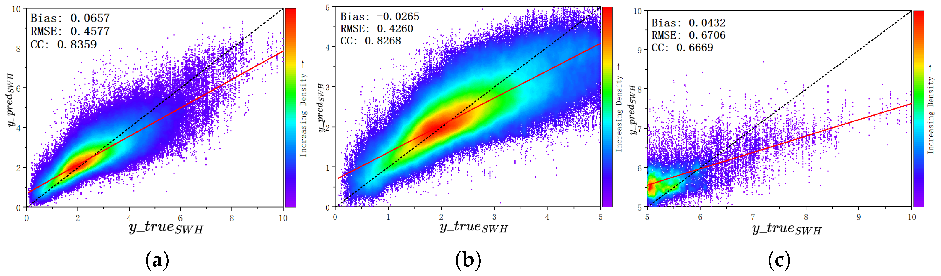
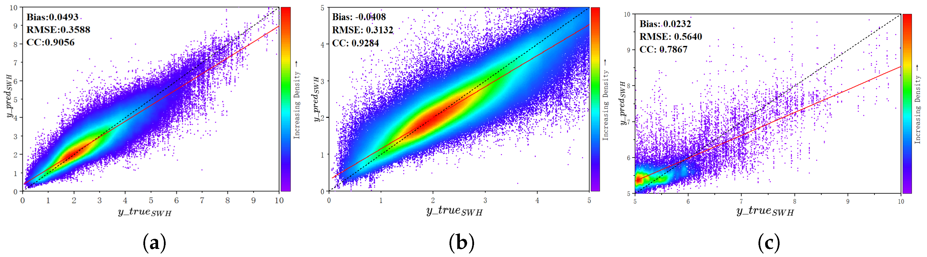
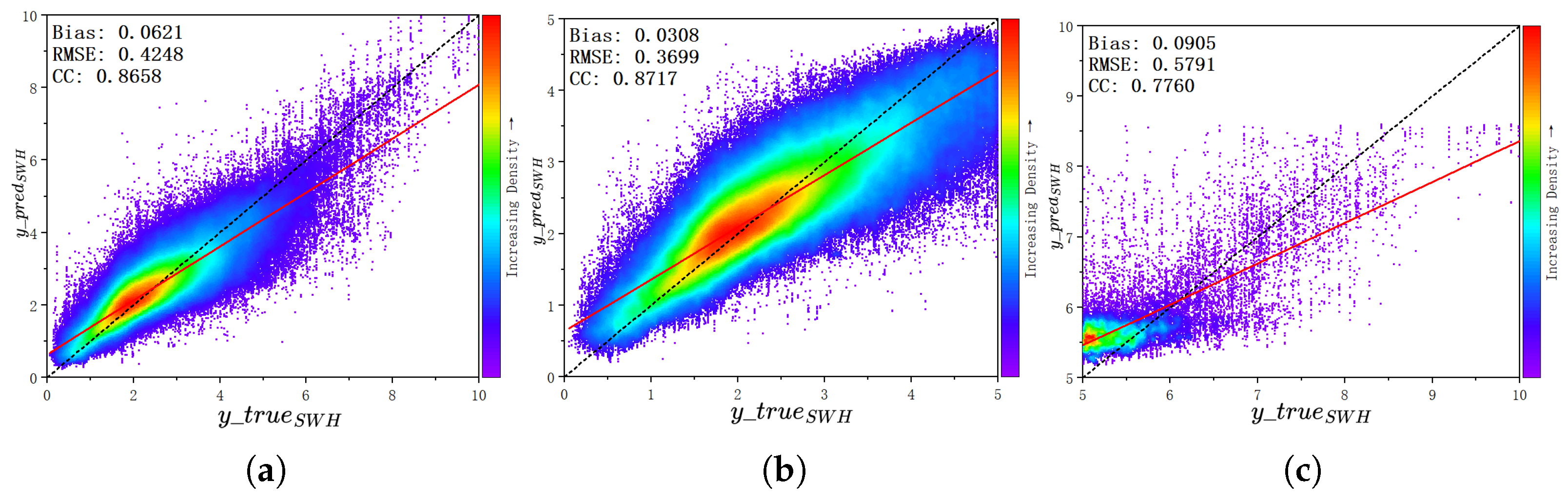
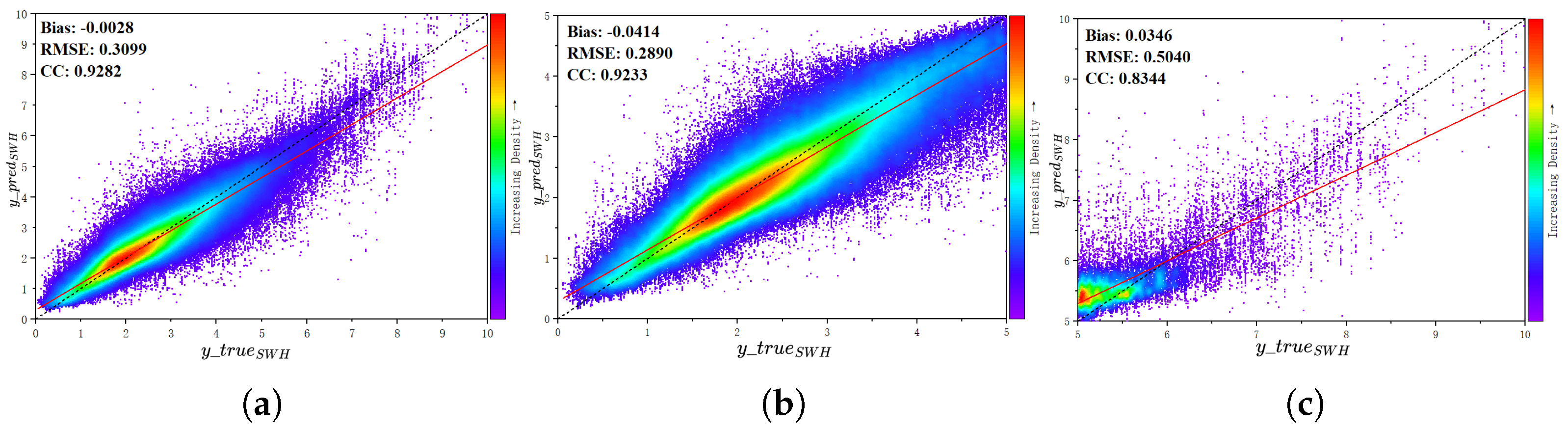
Figure 2, Figure 3, Figure 4 and Figure 5 illustrate the retrieval performance on the test set using scatter density plots of predicted versus true SWH. In these plots, color intensity (purple to red) indicates data density, and evaluation metrics are embedded. The black dashed and red solid lines represent the 1:1 reference and linear regression fit, respectively, highlighting the positive linear relationship between predictions and ground truth.

A detailed examination of the scatter density plots reveals clear differences among the evaluated models. For the single-modality models, namely the baseline Deep Neural Network (Figure 2a) and the standard Transformer (Figure 4a), the data points are more dispersed, and their regression fits deviate more noticeably from the one-to-one reference line, especially in the high sea-state range above 5 m (Figure 2c and Figure 4c). This indicates a systematic tendency to underestimate extreme wave heights. After introducing multimodal inputs, the data distribution becomes more concentrated. The multimodal DNN (Figure 3a) shows a denser core closer to the reference line, although noticeable scatter remains at the upper extremes (Figure 3c). By comparison, the proposed MultTransNet (Figure 5a) achieves the best visual agreement with the reference data, with a tighter high-density region and a smaller regression deviation over the full range. Although some dispersion remains at the highest wave heights, the underestimation observed in the single-modality models is clearly alleviated (Figure 5c).

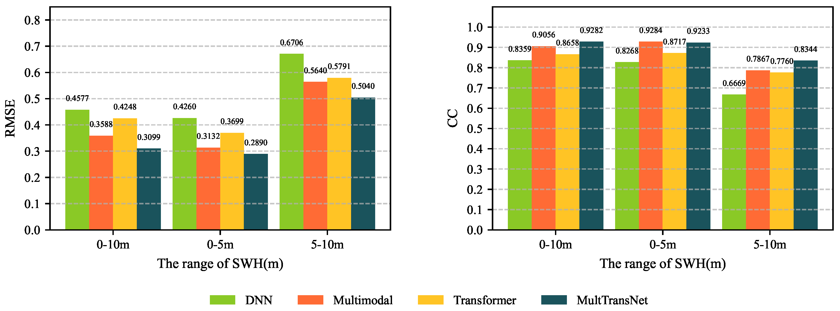
Figure 6 illustrates that the proposed model outperforms others across most SWH ranges, achieving the lowest overall RMSE. It also yields the highest CC, except in the 0–5 m range.

The introduction of multimodal inputs further optimized model performance. Models utilizing multimodal data generally achieved lower RMSE and higher CC values compared to their single-modality counterparts, demonstrating that incorporating spatial scattering information significantly improves retrieval accuracy.

Among all evaluated architectures, the proposed MultTransNet exhibited the most robust overall performance. In the 0–5 m range, it achieved the lowest RMSE of 0.2890, and while its CC of 0.9233 was highly competitive, it was marginally lower than that of the multimodal DNN. However, the true advantage of MultTransNet becomes clearly apparent when considering broader and more complex sea states. Across the comprehensive 0–10 m SWH range, it achieved the absolute best performance, yielding the lowest RMSE of 0.3099 and the highest CC of 0.9282. Furthermore, in the challenging 5–10 m high sea state range, it consistently outperformed all other baseline models in both metrics. Quantitatively, within the full 0–10 m range, MultTransNet demonstrated a 27.05% reduction in RMSE and a 7.21% improvement in CC compared to the single-modality Transformer. This highlights the significant advantage of integrating multimodal data fusion into the Transformer architecture to handle complex marine environments.

This advantage can be understood from the complementary information provided by the two modalities. Compared with the unimodal models, the multimodal architectures benefit from both the physically interpretable auxiliary parameters and the spatial scattering structures contained in the DDM images. As a result, multimodal fusion improves not only the global retrieval accuracy but also the model’s ability to reduce systematic underestimation and preserve spatial consistency under high sea-state conditions. The stronger performance of MultTransNet relative to both the single-modality Transformer and the multimodal DNN further indicates that the benefit of multimodal fusion is most effectively realized when combined with Transformer-based global dependency modeling.

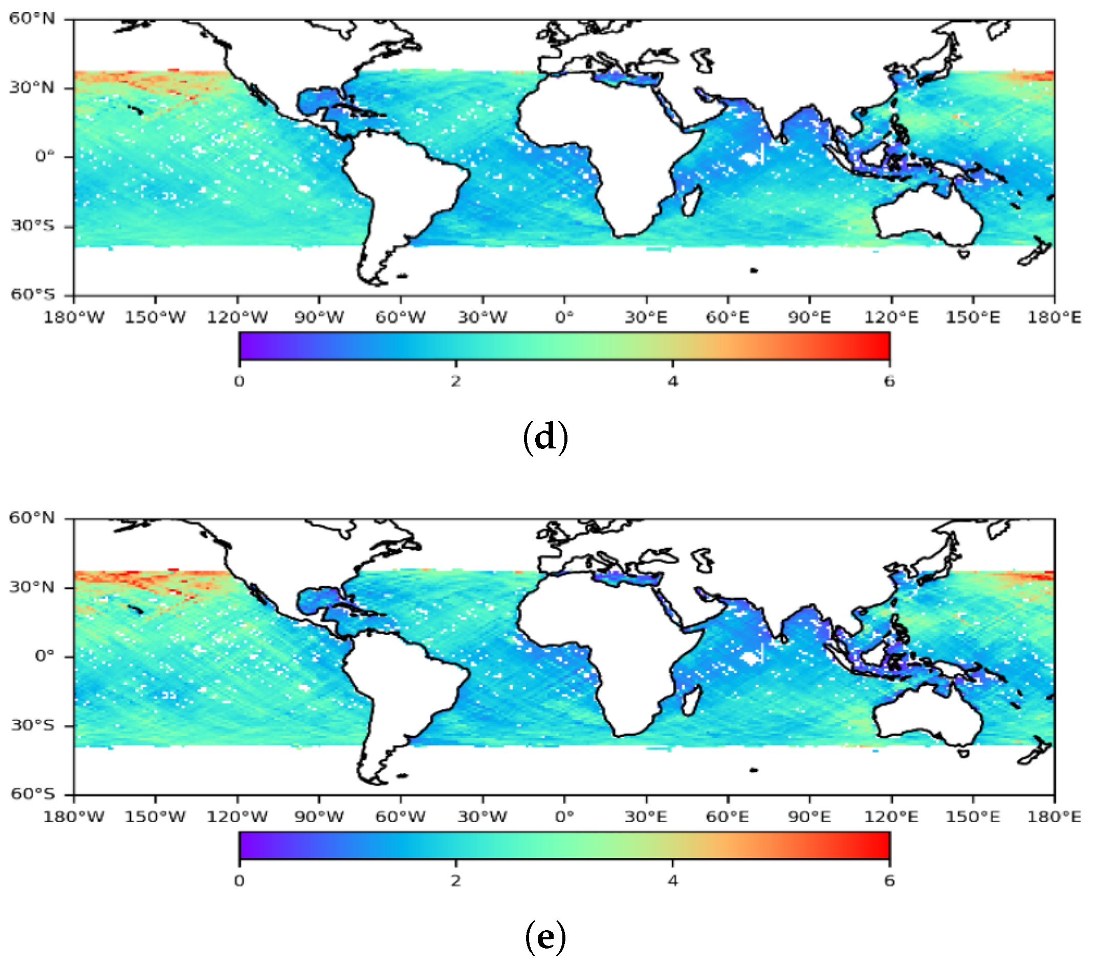
Figure 7 presents the global SWH distributions for the single-modality DNN, single-modality Transformer, multimodal DNN, MultTransNet, and the ERA5 reference data.

The results indicate that the global SWH distribution map generated by the multimodal Transformer model exhibits a high degree of spatial consistency with the ERA5 reference map. This suggests that the combination of the Transformer architecture and multimodal inputs can effectively capture global SWH trends. In contrast, the distribution maps from the other models show a lower degree of concordance with the ERA5 data. This is particularly evident in regions with significant wave heights, where their prediction errors are more pronounced.

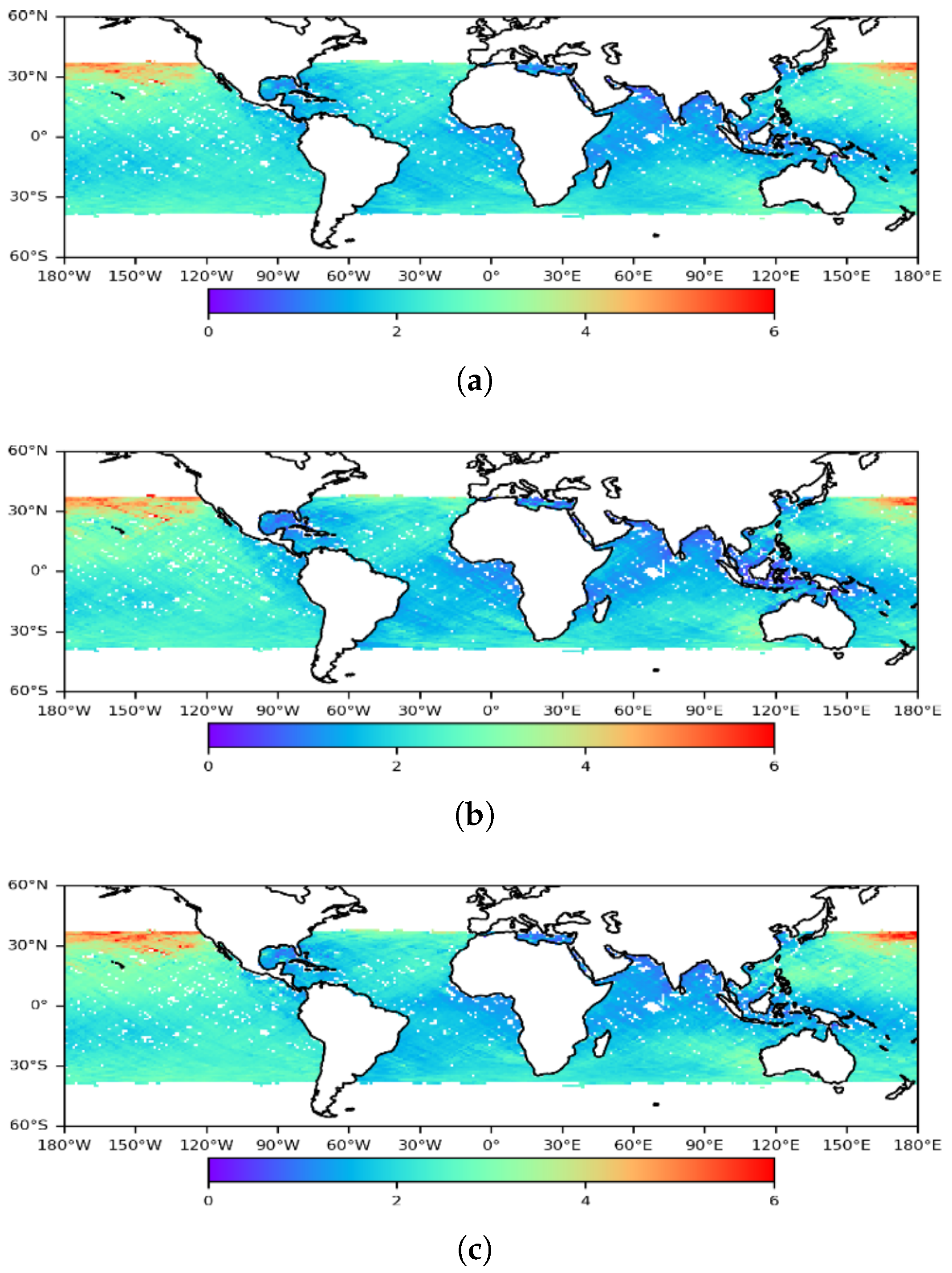
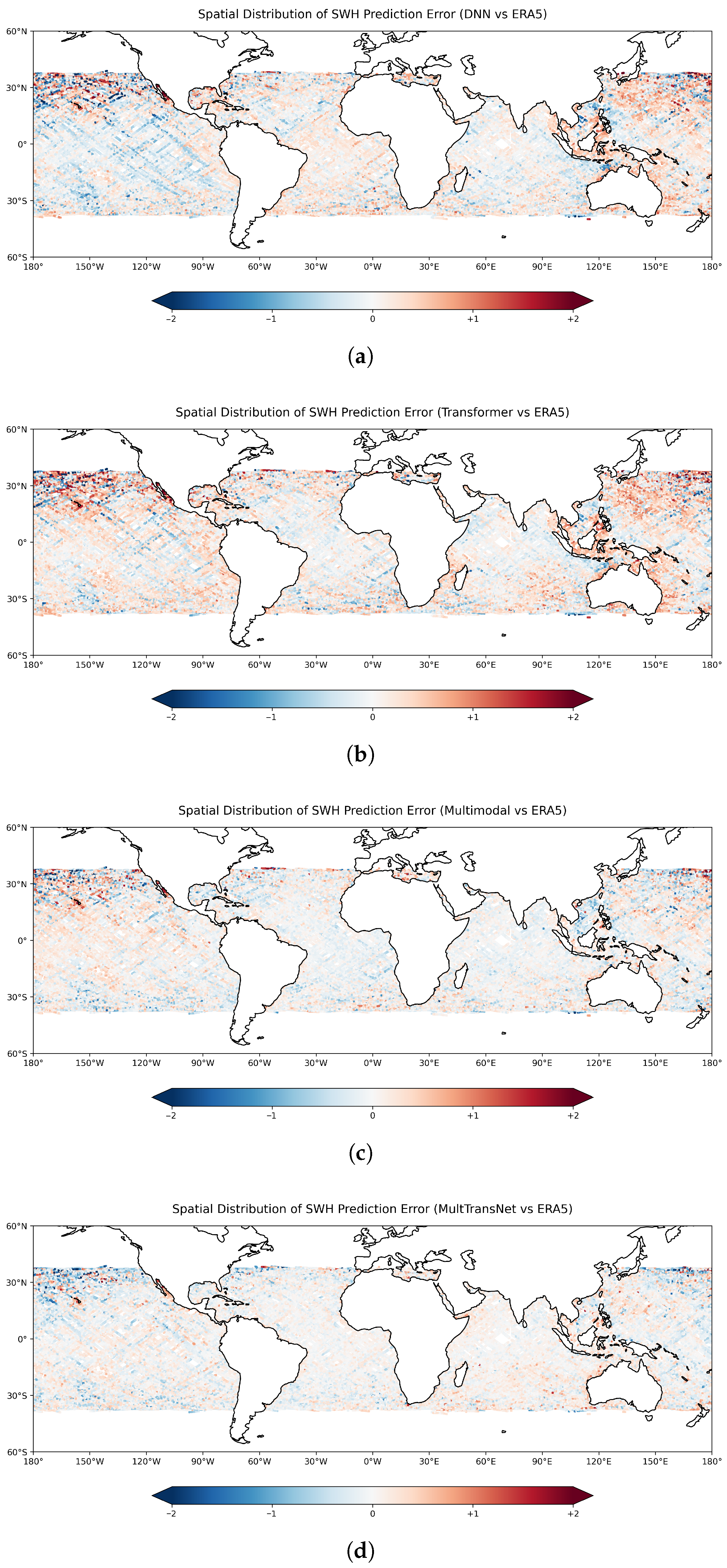
Figure 8 illustrates the global distributions of prediction errors to visually evaluate the spatial performance of different models. The prediction error is defined as predicted significant wave height minus the ERA5 reference, such that positive values indicate overestimation and negative values indicate underestimation. The study region corresponds to the orbital coverage of the satellite constellation, extending from 38°N to 38°S.

As depicted in Figure 8a, an assessment of the baseline Deep Neural Network reveals pronounced regional biases. Notably, widespread underestimations are observed across the mid-to-low latitude regions near the equator, particularly within the eastern Pacific and Indian Oceans. Furthermore, the higher latitudinal boundaries, especially approaching thirty degrees north in the North Pacific, display a highly chaotic error pattern characterized by a distinct and severe mixture of both overestimations and underestimations.

As shown in Figure 8b, the standard Transformer model exhibits an error distribution that shares certain boundary characteristics with the baseline Deep Neural Network while presenting a distinctly different overall trend. Similar to the aforementioned neural network, it maintains a highly chaotic mixture of severe overestimations and underestimations along the higher latitudinal edges, particularly in the North Pacific. However, across the broader mid-to-low latitude regions and equatorial waters, the error pattern shifts significantly, displaying a pervasive and widespread tendency toward overestimation.

Figure 8c illustrates that the integration of multimodal inputs into the baseline Deep Neural Network yields a visually discernible reduction in the overall magnitude of prediction errors. This improvement indicates the positive effect of incorporating two-dimensional spatial scattering information, demonstrating that a multimodal approach contributes beneficially to the feature representation of the model. However, relying on a standard neural network architecture appears to constrain the full potential of this data fusion. Chaotic mixtures of severe overestimations and underestimations persist prominently along the higher latitudinal boundaries, most notably in the North Pacific. Furthermore, a widespread pattern of mild overestimation remains evident across the vast equatorial and mid-latitude regions.

Finally, Figure 8d demonstrates that the proposed MultTransNet achieves a visibly improved error distribution compared to the aforementioned baseline architectures. The spatial extent and intensity of both the severe overestimation and underestimation clusters are noticeably reduced, with a substantially larger proportion of the global observation area converging toward a near-zero error. This improvement is particularly evident across the broad equatorial and mid-latitude oceans, where the pervasive biases observed in earlier models are largely neutralized. However, it is important to note that spatial discrepancies are not entirely eliminated. Slight residual underestimations and minor chaotic error patterns persist at the extreme latitudinal edges of the observation coverage, most notably in portions of the North Pacific. Nevertheless, the overall spatial consistency is enhanced.

Despite these improvements, we acknowledge that the model performance remains limited under extreme sea-state conditions, primarily due to both reduced signal sensitivity and the scarcity of high sea-state samples in the training dataset.

4.3. Case Study Under High Sea-State Conditions

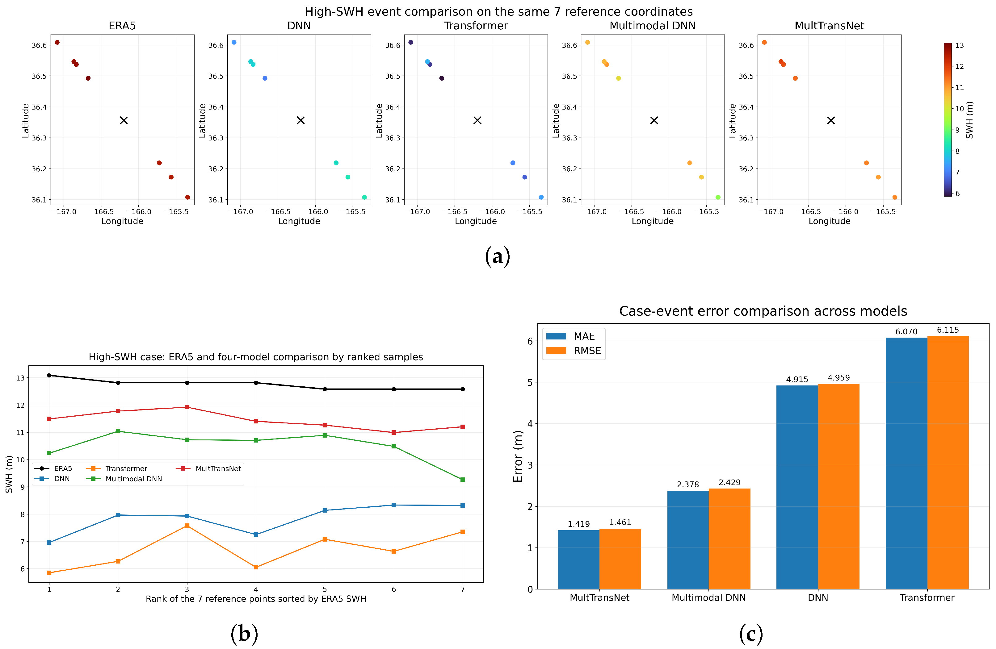
To further evaluate the performance of the proposed model under extreme sea-state conditions, a representative high-SWH event was selected for case analysis. The event occurred at 03:26 UTC on 10 January 2023 in the North Pacific, centered approximately at 36.36°N, 166.20°W. The corresponding ERA5 significant wave height reached 13.27 m, which is substantially higher than the 99.9th percentile value of 9.22 m for the January 2023 dataset, indicating that this event can be regarded as a typical extreme high sea-state case. Moreover, within a $\pm 1°$ spatial window around the event center at the same observation time, 27 matched samples were identified, with SWH values ranging from 12.47 m to 13.27 m and an average of 12.91 m. This indicates that the occurrence of high sea-state conditions over this region at that time was highly probable, confirming that the selected case is representative and physically meaningful rather than being caused by an isolated abnormal sample.

To further compare the retrieval capability of different models under high sea-state conditions, seven representative samples from this event were selected for detailed analysis. Figure 9a presents the spatial comparison between ERA5 and the four models for these samples. As shown in the figure, ERA5 exhibits a pronounced high-wave pattern, with several sample points exceeding 13 m. All four models reproduce the overall high-wave characteristics to some extent; however, clear differences remain in their ability to capture the wave-height magnitude. The DNN and the single-modality Transformer show evident underestimation over most high-wave samples, particularly near the largest values. The multimodal DNN alleviates this deficiency to a certain degree, whereas the proposed MultTransNet yields predictions that are visually closest to the ERA5 reference in both magnitude level and spatial variation. This result suggests that the integration of multimodal information and Transformer-based global feature modeling is more effective for representing high sea-state conditions.

Figure 9b further compares the seven samples after sorting them in descending order according to the ERA5 SWH values. It can be observed that the prediction curves of the DNN and the single-modality Transformer remain consistently below the ERA5 curve, revealing a marked tendency to underestimate high sea states. Although the multimodal DNN still exhibits some deviation, it follows the relative variation among the samples more effectively. In contrast, the MultTransNet predictions remain consistently closer to the ERA5 values across all ranked samples, demonstrating stronger capability in preserving both the peak magnitude and the sample-to-sample variation pattern. This again confirms that multimodal fusion combined with the Transformer architecture enhances model robustness under complex marine conditions.

For a quantitative comparison, Figure 9c shows the MAE and RMSE of the four models over the same seven samples. Among all compared methods, MultTransNet achieves the best performance, with an MAE of 1.419 m and an RMSE of 1.461 m. The multimodal DNN ranks second, with an MAE of 2.378 m and an RMSE of 2.429 m. In contrast, the DNN and the single-modality Transformer produce substantially larger errors, with MAE/RMSE values of 4.915/4.959 m and 6.070/6.115 m, respectively. These quantitative results are fully consistent with the qualitative observations from Figure 9a,b, indicating that the proposed MultTransNet is more effective in suppressing the underestimation of extreme wave heights and provides superior retrieval accuracy in high sea-state scenarios.

Overall, the case study demonstrates that the proposed MultTransNet not only outperforms the baseline models in global statistical evaluations but also exhibits stronger reliability and adaptability in representative extreme sea-state events. This further supports its potential for GNSS-R-based SWH retrieval in complex and high-impact marine environments.

5. Conclusions and Future Directions

This study introduces a highly efficient SWH retrieval methodology utilizing spaceborne GNSS-R data to address existing limitations in feature selection, temporal dependency modeling, and single-modality constraints. By integrating an automatic mechanism for critical feature selection, an advanced sequence modeling architecture, and a multimodal data fusion approach, the proposed methodology comprehensively enhances retrieval accuracy and robustness under complex marine environments.

Specifically, an XGBoost-based iterative feature selection algorithm was developed to systematically evaluate feature importance and inter-feature correlations, effectively eliminating redundant variables and optimizing the input predictor set. To capture long-range temporal dependencies along satellite ground tracks, a Transformer-based retrieval model was designed, utilizing self-attention mechanisms and positional encoding. This architecture demonstrated significant advantages over the baseline Deep Neural Network, reducing the RMSE by 8.91% and increasing the CC by 4.05%. Furthermore, the framework was extended into the proposed MultTransNet by fusing 2D Delay–Doppler Map images with 1D auxiliary parameters. This multimodal integration further improved prediction accuracy, achieving a 27.05% reduction in RMSE and a 7.21% increase in CC compared to its single-modality counterpart, while demonstrating exceptional consistency under high sea-state conditions.

Despite the substantial improvements achieved by MultTransNet, the rapid advancement of satellite remote sensing presents ample opportunities for further refinement. Future research will prioritize enhancing model generalization and interpretability, particularly in challenging oceanic environments. One key direction involves the integration of multi-source observations, fusing GNSS-R measurements with data from Synthetic Aperture Radar, ocean buoys, and airborne platforms to improve adaptability across diverse sea states. Additionally, addressing the underrepresentation of extreme high sea-state events in training datasets remains critical. Employing techniques such as data augmentation, few-shot learning, and dynamically adjusting loss function weights toward high-wave-height samples will be explored to optimize extreme value predictions. Finally, integrating data-driven machine learning with physics-based models through physics-informed regularization will be investigated. This ensures that the retrieval outputs strictly adhere to physical oceanographic principles, thereby simultaneously enhancing the robustness, reliability, and interpretability of the global SWH retrieval framework.

References

1. Wang, H.; Yang, J.; Zhu, J.; Ren, L.; Liu, Y.; Li, W.; Chen, C. Estimation of Significant Wave Heights from ASCAT Scatterometer Data via Deep Learning Network. Remote Sens. 2021, 13, 195. [Google Scholar] [CrossRef] [Scilit]
2. Soulat, F.; Caparrini, M.; Germain, O.; Lopez-Dekker, P.; Taani, M.; Ruffini, G. Sea state monitoring using coastal GNSS-R. Geophys. Res. Lett. 2004, 31, 21303. [Google Scholar] [CrossRef] [Scilit]
3. Shah, R.; Garrison, J.L.; Egido, A.; Ruffini, G. Bistatic Radar Measurements of Significant Wave Height Using Signals of Opportunity in L-, S-, and Ku-Bands. IEEE Trans. Geosci. Remote Sens. 2016, 54, 826–841. [Google Scholar] [CrossRef] [Scilit]
4. Zheng, C.W.; Li, C.Y. Variation of the wave energy and significant wave height in the China Sea and adjacent waters. Renew. Sustain. Energy Rev. 2015, 43, 381–387. [Google Scholar] [CrossRef] [Scilit]
5. Bu, J.; Liu, X.; Wang, Q.; Li, L.; Zuo, X.; Yu, K.; Huang, W. Ocean Remote Sensing Using Spaceborne GNSS-Reflectometry: A Review. IEEE J. Sel. Top. Appl. Earth Obs. Remote Sens. 2024, 17, 13047–13076. [Google Scholar] [CrossRef] [Scilit]
6. Jia, Y.; Lin, M.; Zhang, Y. Evaluations of the Significant Wave Height Products of HY-2B Satellite Radar Altimeters. Mar. Geod. 2020, 43, 396–413. [Google Scholar] [CrossRef] [Scilit]
7. Albuquerque, J.; Antolínez, J.A.; Rueda, A.; Méndez, F.J.; Coco, G. Directional correction of modeled sea and swell wave heights using satellite altimeter data. Ocean Model. 2018, 131, 103–114. [Google Scholar] [CrossRef] [Scilit]
8. Ichikawa, K.; Wang, X.F.; Tamura, H. Capability of Jason-2 Subwaveform Retrackers for Significant Wave Height in the Calm Semi-Enclosed Celebes Sea. Remote Sens. 2020, 12, 3367. [Google Scholar] [CrossRef] [Scilit]
9. Pramudya, F.S.; Pan, J.; Devlin, A.T. Estimation of Significant Wave Height of Near-Range Traveling Ocean Waves Using Sentinel-1 SAR Images. IEEE J. Sel. Top. Appl. Earth Obs. Remote Sens. 2019, 12, 1067–1075. [Google Scholar] [CrossRef] [Scilit]
10. Altiparmaki, O.; Kleinherenbrink, M.; Naeije, M.; Slobbe, C.; Visser, P. SAR Altimetry Data as a New Source for Swell Monitoring. Geophys. Res. Lett. 2022, 49, e2021GL096224. [Google Scholar] [CrossRef] [Scilit]
11. Yang, S.; Jin, S.; Jia, Y.; Ye, M. Significant Wave Height Estimation from Joint CYGNSS DDMA and LES Observations. Sensors 2021, 21, 6123. [Google Scholar] [CrossRef] [Scilit]
12. Bu, J.; Yu, K. Significant Wave Height Retrieval Method Based on Spaceborne GNSS Reflectometry. IEEE Geosci. Remote Sens. Lett. 2022, 19, 1503705. [Google Scholar] [CrossRef] [Scilit]
13. Bu, J.; Yu, K. A New Integrated Method of CYGNSS DDMA and LES Measurements for Significant Wave Height Estimation. IEEE Geosci. Remote Sens. Lett. 2022, 19, 1505605. [Google Scholar] [CrossRef] [Scilit]
14. Afzal, M.S.; Kumar, L.; Chugh, V.; Kumar, Y.; Zuhair, M. Prediction of significant wave height using machine learning and its application to extreme wave analysis. J. Earth Syst. Sci. 2023, 132, 51. [Google Scholar] [CrossRef] [Scilit]
15. Bu, J.; Wang, Q.; Liu, X.; Li, L.; Zhang, Y.; Huang, W. Ocean Swell Height Estimation From Spaceborne GNSS-R Data Using Tree Model Based Machine Learning Methods. In Proceedings of the 2024 IEEE/OES Thirteenth Current, Waves and Turbulence Measurement (CWTM), Wanchese, NC, USA, 18–20 March 2024; pp. 1–5. [Google Scholar] [CrossRef] [Scilit]
16. Bu, J.; Yu, K.; Ni, J.; Huang, W. Combining ERA5 data and CYGNSS observations for the joint retrieval of global significant wave height of ocean swell and wind wave: A deep convolutional neural network approach. J. Geod. 2023, 97, 81. [Google Scholar] [CrossRef] [Scilit]
17. Aleissaee, A.A.; Kumar, A.; Anwer, R.M.; Khan, S.; Cholakkal, H.; Xia, G.S.; Khan, F.S. Transformers in Remote Sensing: A Survey. Remote Sens. 2023, 15, 1860. [Google Scholar] [CrossRef] [Scilit]
18. Qiao, X.; Huang, W. Global Significant Wave Height Retrieval from Spaceborne GNSS-R Using Transformers. In Proceedings of the OCEANS 2024—Singapore, Singapore, 14–18 April 2024; pp. 1–7. [Google Scholar] [CrossRef] [Scilit]
19. Han, X.; Wang, X.; He, Z.; Wu, J. Significant Wave Height Retrieval in Tropical Cyclone Conditions Using CYGNSS Data. Remote Sens. 2024, 16, 4782. [Google Scholar] [CrossRef] [Scilit]
20. Cai, M.; Cheng, X.; He, S.; Cui, Y.; Xie, H.; Pang, J.; Li, S. A Deep Neural Networks-based Significant Wave Height Inversion Method for GNSS-R Signals. In Proceedings of the 2024 4th International Conference on Neural Networks, Information and Communication Engineering (NNICE), Guangzhou, China, 19–21 January 2024; pp. 1208–1211. [Google Scholar] [CrossRef] [Scilit]
21. Zhou, Z.; Duan, B.; Ren, K.; Ni, W.; Cao, R. Enhancing Significant Wave Height Retrieval with FY-3E GNSS-R Data: A Comparative Analysis of Deep Learning Models. Remote Sens. 2024, 16, 3468. [Google Scholar] [CrossRef] [Scilit]
22. Qin, L.; Li, Y. Significant Wave Height Estimation Using Multi-Satellite Observations from GNSS-R. Remote Sens. 2021, 13, 4806. [Google Scholar] [CrossRef] [Scilit]
23. Jinwei, B.; Kegen, Y.; Shuai, H. Construction of spaceborne GNSS-R ocean waves significant wave height retrieval model. Acta Geod. Cartogr. Sin. 2022, 51, 1920–1930. [Google Scholar] [CrossRef]
24. Bu, J.; Yu, K.; Han, S.; Qian, N.; Lin, Y.; Wang, J. Retrieval of Sea Surface Rainfall Intensity Using Spaceborne GNSS-R Data. IEEE Trans. Geosci. Remote Sens. 2022, 60, 1–16. [Google Scholar] [CrossRef] [Scilit]
25. Reynolds, J.; Clarizia, M.P.; Santi, E. Wind Speed Estimation From CYGNSS Using Artificial Neural Networks. IEEE J. Sel. Top. Appl. Earth Obs. Remote Sens. 2020, 13, 708–716. [Google Scholar] [CrossRef] [Scilit]
26. Asgarimehr, M.; Arnold, C.; Weigel, T.; Ruf, C.; Wickert, J. GNSS reflectometry global ocean wind speed using deep learning: Development and assessment of CyGNSSnet. Remote Sens. Environ. 2022, 269, 112801. [Google Scholar] [CrossRef] [Scilit]
27. Clarizia, M.P.; Ruf, C.S. Statistical Derivation of Wind Speeds From CYGNSS Data. IEEE Trans. Geosci. Remote Sens. 2020, 58, 3955–3964. [Google Scholar] [CrossRef] [Scilit]
28. Clarizia, M.P.; Ruf, C.S.; Jales, P.; Gommenginger, C. Spaceborne GNSS-R Minimum Variance Wind Speed Estimator. IEEE Trans. Geosci. Remote Sens. 2014, 52, 6829–6843. [Google Scholar] [CrossRef] [Scilit]
Figure 1. Overall architecture of the proposed MultTransNet.
Remotesensing 18 01351 g001
Figure 2. Density scatter plots of predicted versus true SWH for the DNN across different measurement ranges. (a) shows the results over the full SWH range of 0–10 m; (b) covers the low range of 0–5 m; and (c) covers the high range of 5–10 m. Bias, RMSE, and CC are annotated in each subfigure.
Remotesensing 18 01351 g002
Figure 3. Density scatter plots of predicted versus true SWH for the multimodal DNN across different measurement ranges. The results are shown for three SWH ranges: (a) the full range (0–10 m), (b) the low range (0–5 m), and (c) the high range (5–10 m). Bias, RMSE, and CC metrics are provided.
Remotesensing 18 01351 g003
Figure 4. Density scatter plots of predicted versus true SWH for the standard single-modality Transformer across different measurement ranges. The evaluation is split into three distinct SWH ranges: (a) 0–10 m (full range), (b) 0–5 m (low range), and (c) 5–10 m (high range).
Remotesensing 18 01351 g004
Figure 5. Density scatter plots of predicted versus true SWH for the proposed MultTransNet across different measurement ranges. The results are presented for three SWH ranges: (a) 0–10 m (full range), (b) 0–5 m (low range), and (c) 5–10 m (high range).
Remotesensing 18 01351 g005
Figure 6. Overall comparison of model performance based on RMSE and CC metrics.
Remotesensing 18 01351 g006
Figure 7. Global spatial distribution of retrieved SWH for all evaluated models and the ERA5 reference data. (a) DNN, (b) Multimodal, (c) Transformer, (d) MultTransNet, (e) ERA5.
Remotesensing 18 01351 g007aRemotesensing 18 01351 g007b
Figure 8. Global spatial distribution of prediction errors (Predicted SWH - ERA5 SWH) for the evaluated models. (a) DNN, (b) Transformer, (c) Multimodal, (d) MultTransNet. Blue regions indicate underestimation, while red regions indicate overestimation.
Remotesensing 18 01351 g008
Figure 9. Case study of model performance under high sea-state conditions. (a) Spatial comparison of ERA5 and the predicted SWH values from different models for the selected high sea-state case. (b) Ranked comparison of ERA5 and model-predicted SWH values for the same seven representative samples. (c) MAE and RMSE comparison of different models for the selected high sea-state case.
Remotesensing 18 01351 g009