Mapping Building-Level Monthly CO₂ Emissions of Different Functions: A Case Study of England

Highlights

What are the main findings?

• Distinct functional buildings exhibit unique patterns of carbon emission intensity.
• Building carbon emissions exhibit significant spatiotemporal heterogeneity.

What are the implications of the main findings?

• The framework enables scalable, fine-resolution disaggregation of building carbon emissions.
• The findings may support government decisions in urban planning and spatial policy, contributing to low-carbon development goals.

Abstract

Understanding carbon dioxide (CO₂) emissions from buildings is critical for shaping effective policies toward sustainable urban development. Previous studies mainly applied bottom-up methods for small areas or top-down downscaling at national, provincial or grid scales. However, limited research has explored the relationship between building functions and CO₂ emissions at a larger scale. To bridge this gap, this study employed ridge regression to disaggregate monthly CO₂ emissions to the level of different functional buildings across England in 2022 and investigated the relationship between building functions and CO₂ emissions. Results show that commercial buildings rank highest in CO₂ intensity, reaching 1.49 kg per volume in February, while residential buildings rank lowest, reaching 0.25 kg per volume in July at the national scale, and industrial buildings have the largest total emissions. In addition, regional disparities in economic development and industrial structure contribute to emission differences among buildings of the same function. Temporally, all functional buildings exhibited lower emissions during summer compared to winter. Overall, this study offers a scalable and interpretable framework for understanding urban carbon emissions at high spatial and functional granularity. The findings may offer valuable insights to support government decision-making in urban planning and spatial policy design, thereby contributing to low-carbon development goals.

1. Introduction

The escalating concentration of atmospheric carbon dioxide (CO₂) poses increasingly severe global challenges [1,2]. As a primary anthropogenic greenhouse gas, rising CO₂ levels have intensified the greenhouse effect, leading to global warming and triggering a cascade of environmental consequences, including ecosystem destabilization and a heightened frequency of extreme weather events [3]. Over the past few decades, numerous scholars have conducted valuable research on building CO₂ emissions. A prevalent research perspective focuses on assessing emissions through the building lifecycle. The llifecycleassessment (LCA) approach quantifies the carbon footprint across all stages, including material production, construction, operation, and end-of-life disposal, thus providing a comprehensive estimate of building-related emissions [4,5,6]. For instance, Fan et al. applied the LCA framework to a new university campus to assess CO₂ emissions across material production, transportation, construction, operation, maintenance, and demolition [7]. Similarly, Seyedabadi et al. compared the life cycle carbon emissions of steel and concrete structures under different national building codes [8]. Although this method provides a more complete and accurate carbon footprint, it requires extensive data for each stage of the building liflifecycleeading to computational complexity and high computational time costs, thereby limiting its efficiency for large-scale assessments. To further improve computational efficiency, research institutions have developed generic models that integrate diverse building carbon accounting and energy simulation techniques. Representative tools include One-Click LCA developed by Bionova [9], EnergyPlus [10], PKPM-CES developed by the China Academy of Building Research [11], and Tally developed by Autodesk [12]. These tools can enable multi-scale, lifecycle carbon emission simulation. For example, Liu et al. combined the DeST simulation model with the emission factor method to estimate CO₂ emissions from four million buildings in the Pearl River Delta [13]. Likewise, Grygierek et al. employed EnergyPlus to simulate the lifelifecyclergy consumption of a detached house in Poland over 25 years [14]. Such modeling tools offer greater flexibility for scenario analysis, particularly in large-scale, complex systems where extensive empirical data are lacking. Nonetheless, they still demand large volumes of input data and sophisticated parameterization, which impose high costs on users. It is worth noting that building operational carbon emissions refer to the CO₂ emissions generated from energy consumption during the use phase of buildings, including heating, cooling, lighting, and equipment operation, which generally account for the largest share of total emissions, surpassing embodied emissions from materials and construction due to its long duration and high energy intensity [15]. Moreover, estimating operational emissions is more computationally efficient. Consequently, simplified and accurate assessments of building operational CO₂ emissions remain a focal point for researchers.

The emission factor method is one of the most widely used approaches for large-scale emission estimation, which forms the basis for large-scale assessments of building-related emissions by multiplying activity data with corresponding emission factors [16]. Many researchers have adopted this approach for estimating urban- or regional-scale CO₂ emissions. For example, Ke et al. used China’s central grid emission factors to calculate operational energy-related emissions of residential buildings in the hot-summer, cold-winter region of the Yangtze River Basin [17]. Similarly, Wang et al. estimated building-related CO₂ emissions across 266 Chinese cities by applying the emission factor method to city- and provincial-level energy consumption statistics [18]. Although the emission factor method is efficient, requires relatively few data, and is widely applicable, it struggles to capture heterogeneity across individual buildings, and its accuracy is highly dependent on the spatial and temporal resolution of the emission factors. It is worth noting that these methods tend to struggle to fully characterize the spatial and temporal variations in energy use at finer scales, thereby posing challenges in revealing the dynamic patterns of buildings’ long-term operational performance.

Accurately estimating building carbon emissions across multiple scales and scenarios has also become a key focus in academia. The two primary frameworks are bottom-up modeling and top-down downscaling. Bottom-up modeling estimates emissions by aggregating building-specific data, enabling high-resolution, source-level analysis [19]. For example, Liang et al. developed a high-resolution dataset of building material stocks and embodied carbon emissions for two major Chinese urban agglomerations (2000–2020) using a bottom-up material stock accounting approach [20]. However, this approach relies on high-quality building-level data, which are difficult to obtain at large spatial scales, limiting its applicability in broad-scale studies. Furthermore, top-down downscaling estimates carbon emissions using macro-level indicators such as socioeconomic data and then allocates these estimates to finer spatial scales [21]. For example, Zhao et al. established relationships between provincial building energy consumption and carbon emissions (BECCE), integrating additional covariates to produce China’s 1 km resolution BECCE dataset [22]. Similarly, Wang et al. combined population grids, night-time light data, and GDP to create the first global high-resolution GDP–carbon emission joint dataset [23]. Top-down downscaling is better suited for large-scale estimations. However, low-resolution proxies may limit the spatial and temporal resolution of studies, making it difficult to capture variations in building energy use at finer scales. Xia et al. combined high-resolution remote sensing, building information modeling, and energy consumption data to allocate carbon emissions at the street level, attempting to construct a carbon emission map for Beijing’s building sector [24]. Furthermore, Rodríguez et al. quantitatively analyzed the solar photovoltaic potential across 34 German cities, applying the results to individual buildings [25], aiming to achieve finer spatial scale estimations over a large area. These studies provide substantial evidence for exploring the relationship between buildings and CO₂ emissions at higher spatial resolutions.

Some studies have pointed out that differences in human activities within buildings lead to variations in energy consumption, which in turn result in significant disparities in carbon emissions among different building functions. For example, Guo et al. emphasize the need to develop lifecycle emission reduction strategies tailored to different building types to avoid the limitations of “one-size-fits-all” approaches [26]. Mao et al.’s study highlighted that differences in types of human activities (e.g., residential heating/cooling and industrial energy-intensive production) significantly affect the spatial distribution of carbon emissions [27]. Recently, some studies calculating building CO₂ emissions have begun to account for variations driven by building functions. For example, Sun’s study analyzed the differences in CO₂ emissions between commercial and residential buildings using a spatial econometric model [28]. Similarly, Yu et al. tried to estimate total operational carbon emissions from buildings across 321 Chinese cities, disaggregated by building function and end-use category [29]. Unfortunately, most studies remain at coarse spatial scales and have not achieved fine-scale assessments of building carbon emissions. Due to limitations of traditional methods, obtaining large-scale building functional classification data remains difficult. Therefore, quantitatively revealing the relationship between building functions and CO₂ emissions at fine spatial scales remains challenging.

In summary, although numerous scholars have investigated carbon emissions from buildings, few have explored the profound relationship between building functions and carbon emissions at a finer spatial scale due to the difficulty in obtaining building classification data. It is worth noting that the proliferation of machine learning techniques has enabled large-scale classification of building functions across vast geographic areas [30,31,32]. Building on this foundation, this study employed a ridge regression model to establish monthly CO₂ emission disaggregates for approximately 11.5 million buildings across England in 2022, categorized into five functional types. The model integrates building volume of each type, night-time light data, and EDGAR CO₂ emission grid maps. This study aims to quantify and compare functional differences in building-related CO₂ emissions and to reveal their spatiotemporal distribution patterns. The findings are expected to provide theoretical foundations and actionable insights for targeted emission reduction strategies and sustainable urban planning.

2. Materials and Methods

2.1. Study Area

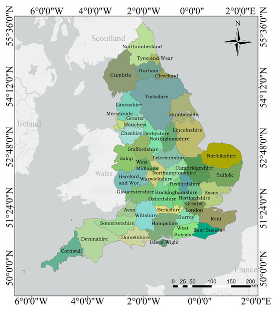
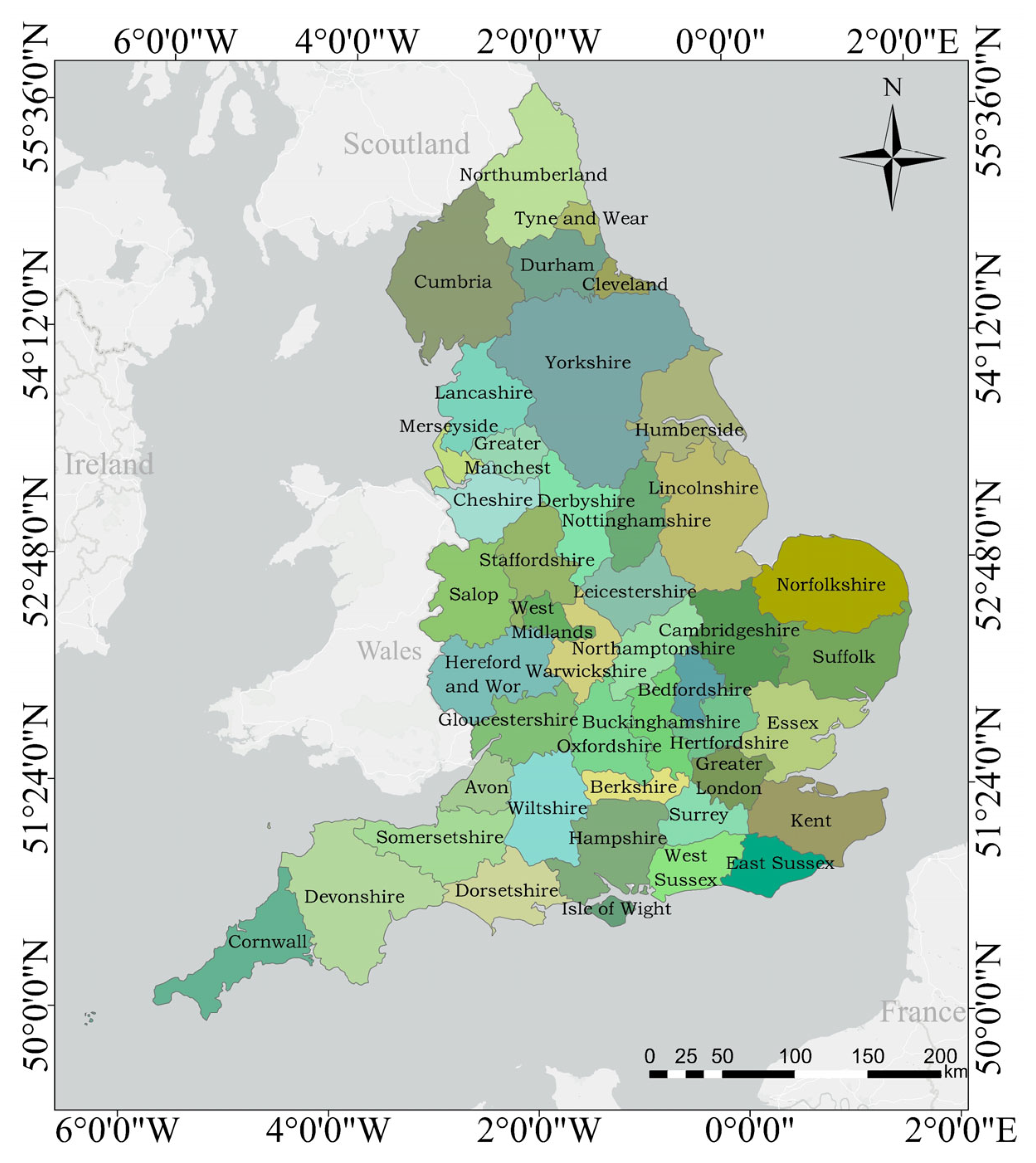
In this study, England was selected as the study area. As shown in Figure 1, England is located in the southeastern part of Great Britain and, together with Scotland, Wales, and Northern Ireland, forms the United Kingdom of Great Britain and Northern Ireland. It is divided into 44 administrative divisions. The UK’s urbanization rate had reached nearly 85% in 2023 [33]. This rapid urban expansion has inevitably contributed to significant CO₂ emissions from buildings. According to a report published by the UK government [34], the estimated CO₂ emissions in the UK were approximately 331 million tons in 2023. To mitigate these emissions, in recent years, England has enacted various low-carbon policies to reduce CO₂ emissions from buildings. The most notable is the revised Climate Change Act of 2019, which set a target of achieving net-zero emissions by 2050 [35]; the Building Regulations, meanwhile, established distinct energy efficiency standards for buildings with different functions [36], providing valuable references for global building carbon reduction. Therefore, England is an ideal region for researching CO₂ emissions from different functional buildings.

Figure 1. The geographical location and spatial distribution of England’s 44 counties.

2.2. Overall Framework

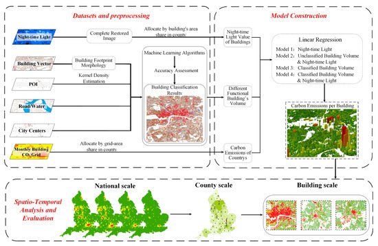
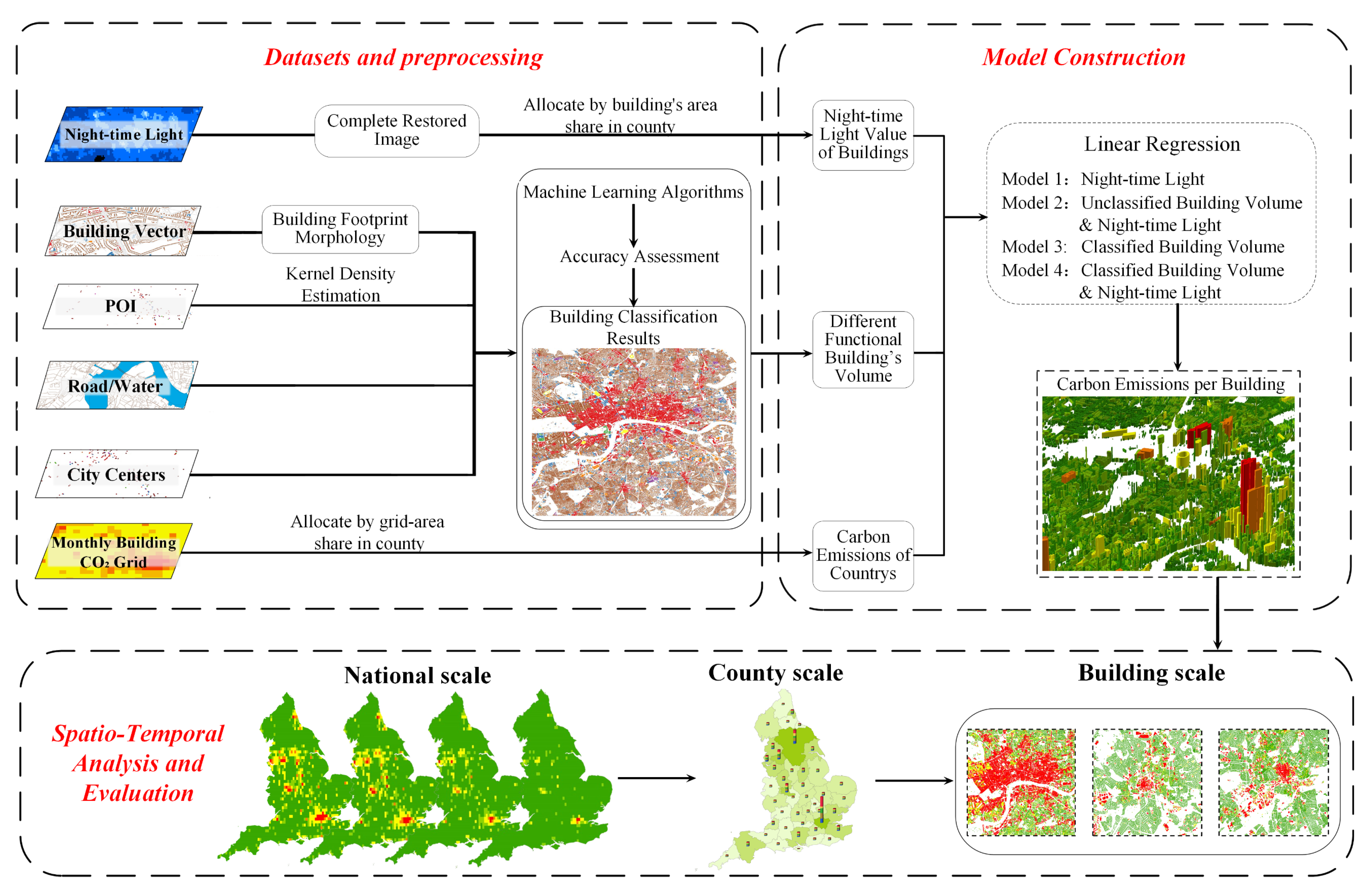
To disaggregate monthly CO₂ emissions at the building level, night-time light and building volume data were used as independent variables, combined with overall EDGAR CO₂ emission data for each spatial unit as the dependent variable, to establish four linear regression models for allocating the monthly CO₂ emissions of individual buildings in England. The overall framework of this study is shown in Figure 2 and can be divided into three parts: (1) Data preparation. We collected and processed the required data for the model input variables. The results of building classification and their corresponding visualizations are provided in the Supplementary Materials. (2) Model construction. We developed four linear regression models using different sets of independent variables. Model performance was validated using multiple evaluation metrics. (3) Results analyses and evaluation. We utilized various indicators to analyze the spatiotemporal characteristics of CO₂ emissions from different functional buildings in England at national-, county-, and building-scales.

Figure 2. The overall framework for CO₂ emission assessment conducted in this study.

2.3. Data Preparation and Processing

2.3.1. Building Vector Data

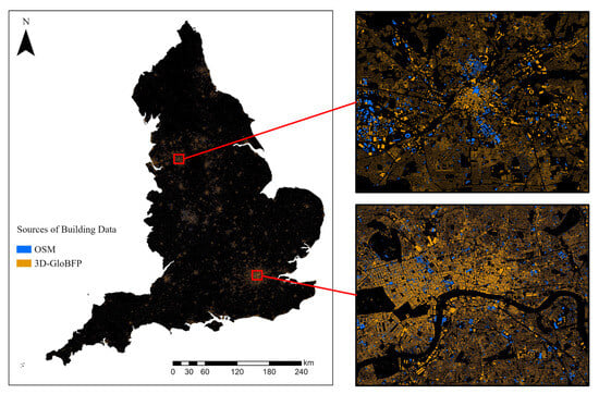
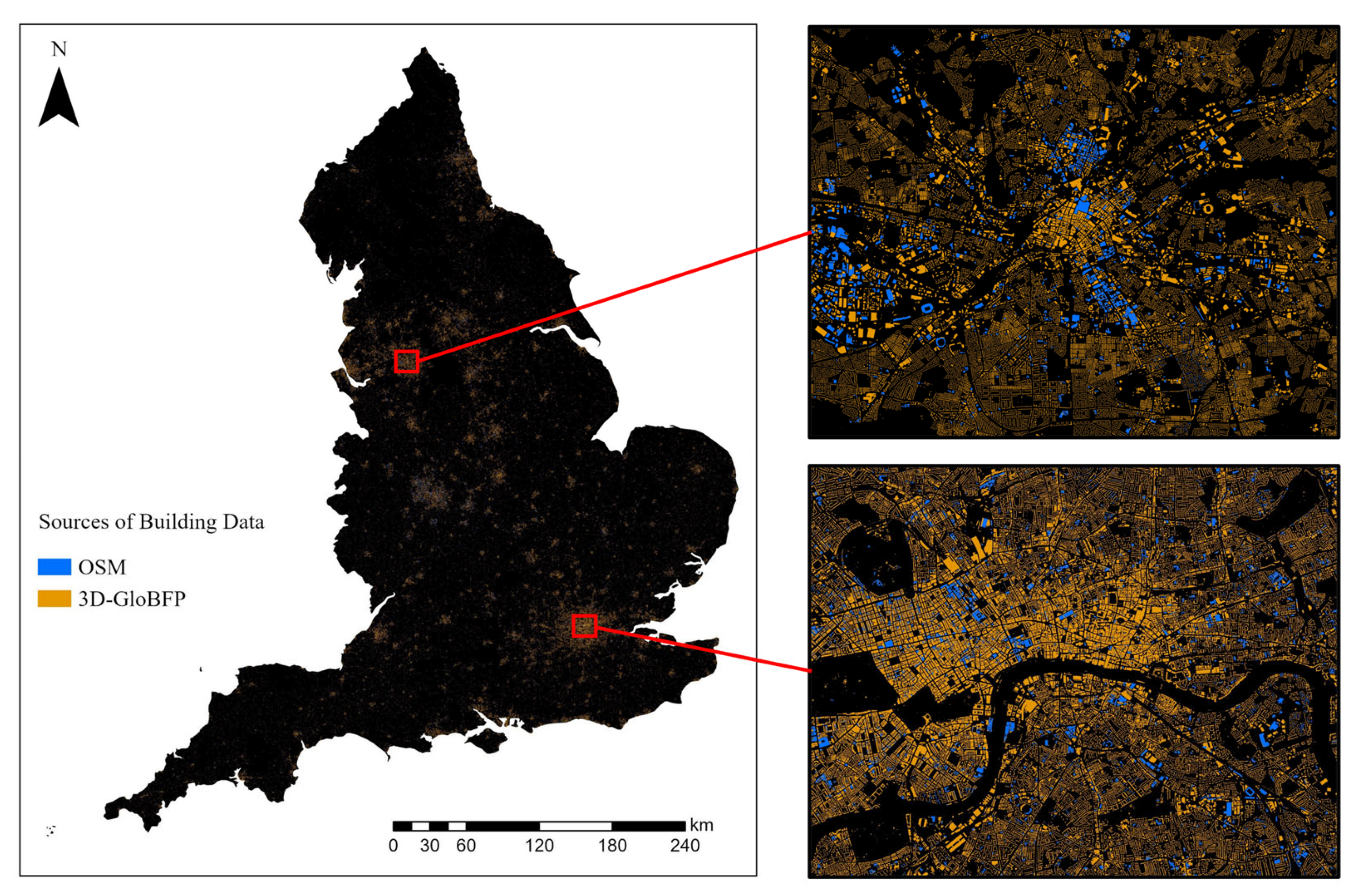
Currently, no publicly available high-quality dataset fully classifies building functions across England. Therefore, this study addressed that gap by generating a consistent, high-resolution dataset essential for subsequent carbon emission modeling and analysis. Two building datasets were used to support building function classification and CO₂ emission mapping at the building level in England. The first dataset is the world’s first building-scale three-dimensional building footprint dataset (3D-GloBFP) [37], which integrates multiple global building datasets for comparison, thereby ensuring comprehensive coverage. This dataset offers extensive coverage of approximately 12 million buildings in England, including footprint and height information, but lacks functional type labels. The second dataset is OpenStreetMap (OSM) [38], which provides a smaller subset of building footprints with known functional types, but the coverage is fragmented and incomplete. It is worth noting that OSM data are crowdsourced, with coverage and quality varying across regions, which may introduce uncertainty. Therefore, we conducted strict filtering and manual inspection of the functional types. As shown in Figure 3, which illustrates the quantity and spatial distribution of buildings from two sources (OSM and 3D-GloBFP), the latter provides more comprehensive building vector coverage compared to OSM. In this study, we used OSM buildings as the training data, while the 3D-GloBFP dataset served as the target buildings to be predicted. For the OSM samples, we selected roughly 570,000 qualified samples and randomly partitioned them into training, test, and validation sets at a ratio of 7:1.5:1.5.

Figure 3. Spatial distribution of building data from two data sources.

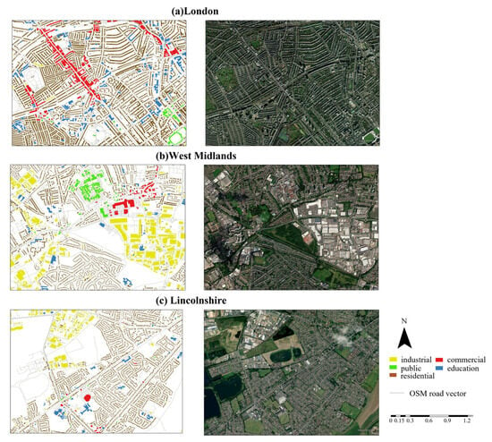
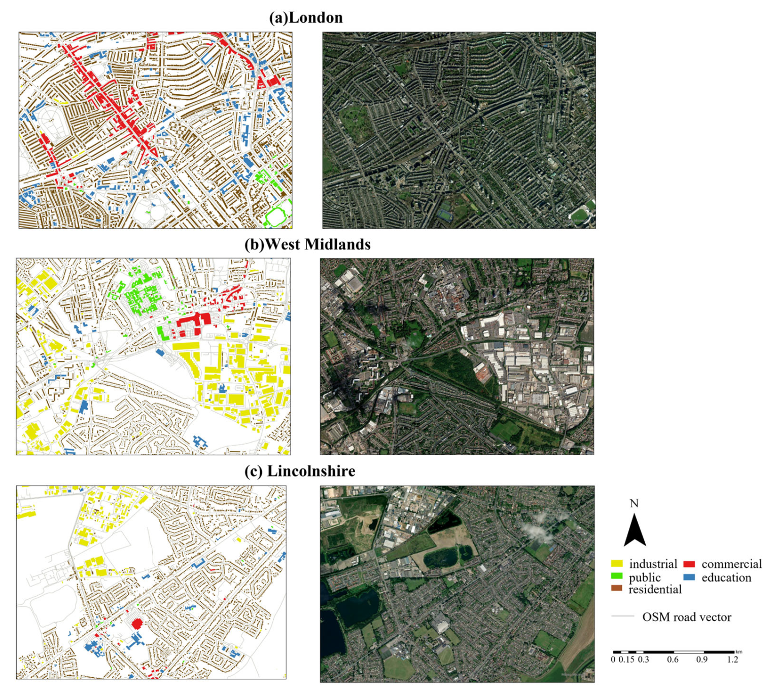
To facilitate model training and ensure consistency, we reclassified the functional building samples from the OpenStreetMap into five unified categories: commercial, education, public, industrial, and residential. Then, we constructed 42 features (encompassing building morphology, distance metrics, and POI kernel density characteristics) using building footprint morphology, POI, road network, and water data for building functional classification. The Supplementary Materials provide detailed descriptions of the label definitions (Tables S1 and S2), the features employed for classification (Table S3), and model performance metrics (Table S1, Figures S1 and S2). Based on evaluation metrics and manual inspection, it is proven that most buildings can be accurately classified. The final classification results are presented in Figure 4. As shown in Figure 4b,c, prominent public buildings such as stadiums were generally well classified. Moreover, educational buildings, such as schools, were also reasonably identified.

Figure 4. Building function classification for representative regions. The right column of figures shows remote sensing images from Google, from the same time period as this study (2022).

2.3.2. Monthly CO₂ Data

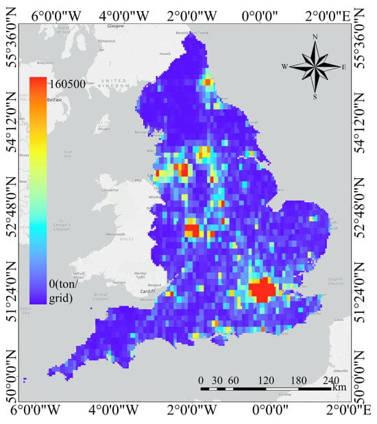
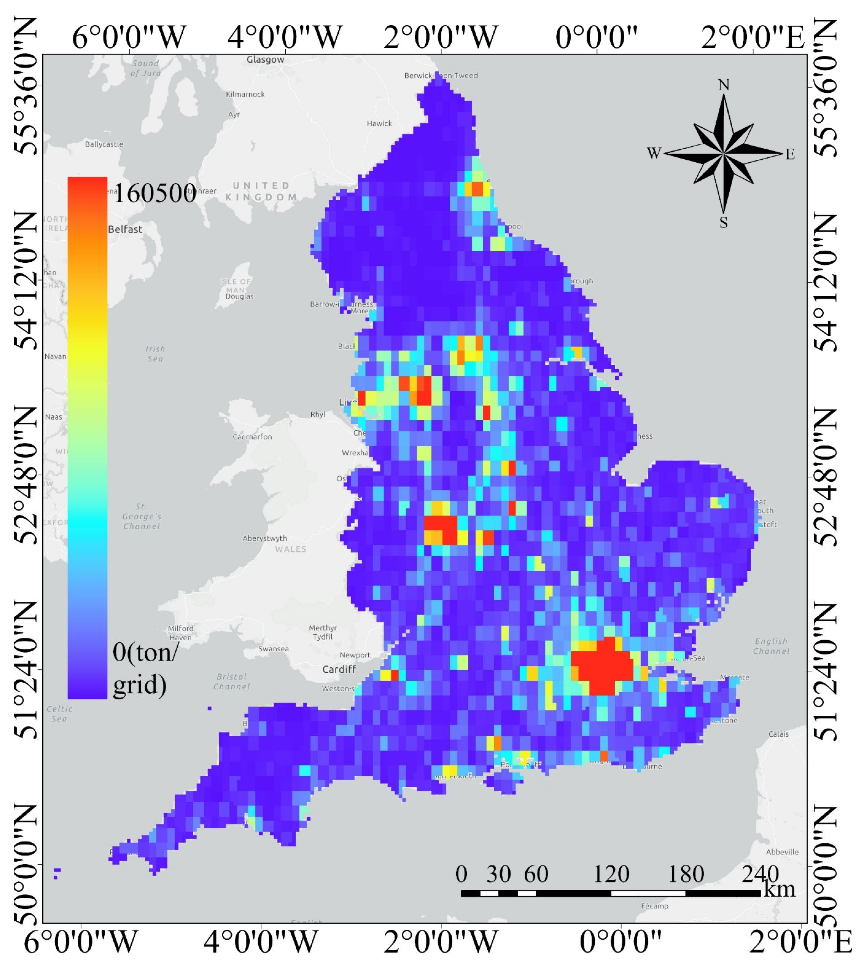
This study used monthly CO₂ emission data for the building energy sector in 2022 obtained from the EDGAR database, as shown in Figure 5. The EDGAR database is provided by the European Commission’s Joint Research Centre (EU-JRC) and the PBL Netherlands Environmental Assessment Agency (PBL) [39]. It offers CO₂ emission data across various sectors, including building, energy, industry, and agriculture, with a spatial resolution of 0.1° × 0.1° and temporal coverage spanning from 1970 to the most recent available year on a monthly basis. The comprehensive coverage, high spatial resolution, and extensive temporal sequence of the EDGAR database make it widely used in climate and environmental research [40,41,42].

Figure 5. EDGAR building energy sector’s grid CO₂ emissions data in December.

This dataset was considered ideal for calculating CO₂ emissions from buildings in this study. Given that the analytical framework operates at spatial units that do not fully align with the original 0.1° × 0.1° resolution of the EDGAR carbon emission data, we reallocated the carbon emission data. Specifically, the carbon emission grids were spatially overlaid and clipped using the boundary of the target spatial units. Subsequently, the CO₂ emissions of each grid cell were proportionally allocated to the target units based on the area of overlap. The calculation formula is shown in Equation (1):

$$C_k=\sum _{\mathrm{i}=0}^{\mathrm{m}}{\mathrm{G}}_{\mathrm{i}}+\sum _{\mathrm{j}=0}^{\mathrm{n}}{\mathrm{G}}_{\mathrm{j}}$$

(1)

where C_k represents total CO₂ emissions of a specific unit k, and m and n represent the number of EDGAR grid cells that are fully and partially contained within unit k, respectively. G_i and G_j denote CO₂ emissions from fully and partially contained grid cells, respectively. The total CO₂ emissions of each unit equal the sum of CO₂ emissions from fully contained grid cells within its boundary and the proportional CO₂ emissions from partially contained grid cells based on their overlapping areas within the unit.

2.3.3. Night-Time Light Data

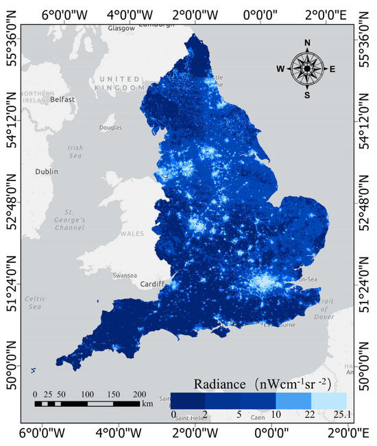
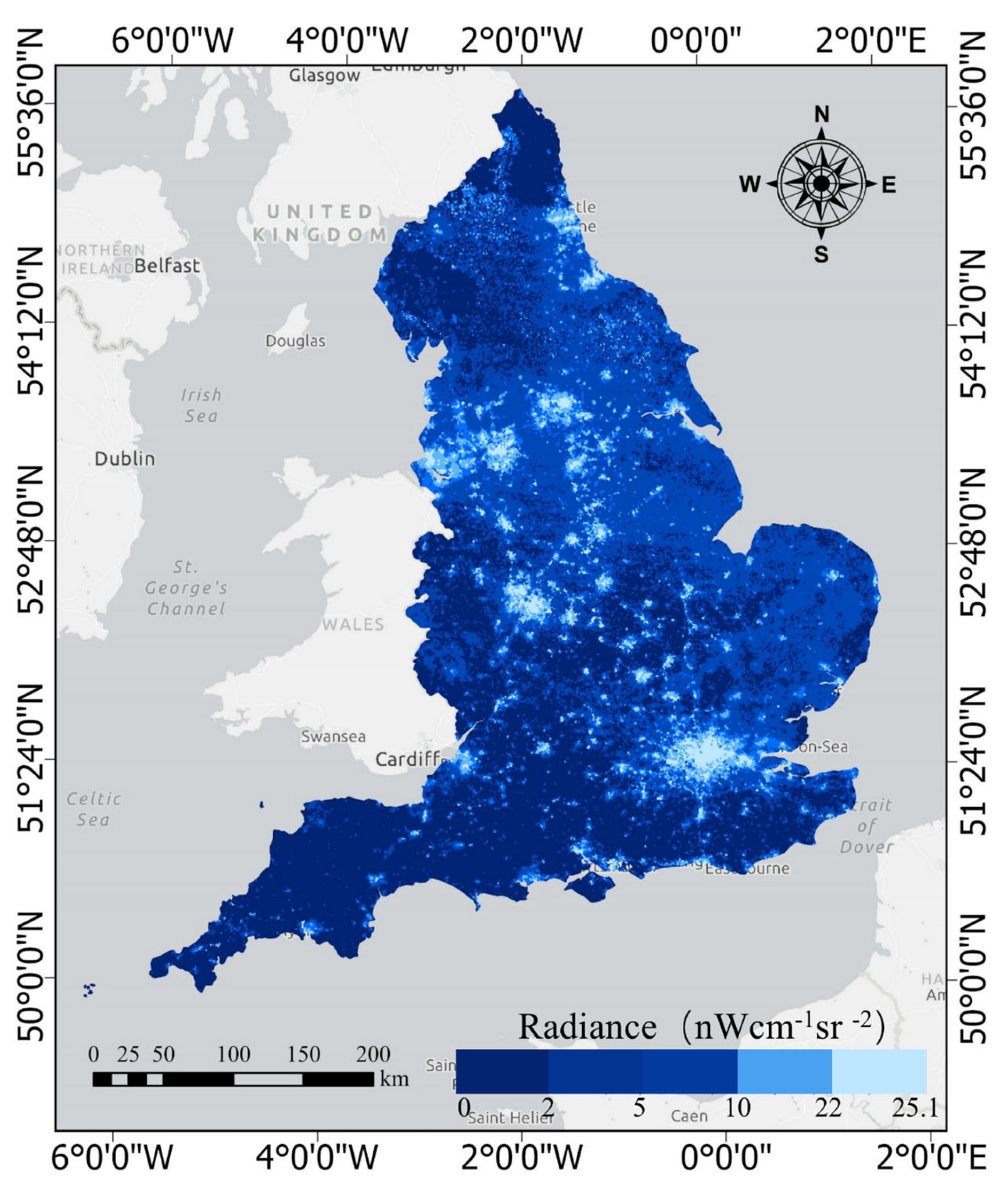
Night-time light imagery reflects human activity through lighting density and is widely used to delineate urban areas, estimate population distribution, and analyze CO₂ emission patterns [43,44]. The primary sources of night-time light data include the Visible Infrared Imaging Radiometer Suite (NPP-VIIRS) Day/Night Band imagery system and the Defense Meteorological Satellite Program/Operational Linescan System (DMSP/OLS) [45]. Compared to DMSP/OLS, NPP-VIIRS provides superior spatial, temporal, and radiometric resolution, eliminating light saturation and detecting fainter emissions, thereby capturing infrastructure use more comprehensively [46,47]. Therefore, this study employed monthly NPP-VIIRS data to assist in disaggregating CO₂ emissions.

To obtain accurate night-time light values, we preprocessed NPP-VIIRS data to eliminate local light saturation. Additionally, we found that July’s night-time light data had a missing rate exceeding 40%, while other months had a missing rate of less than 1%. To address this gap, we employed multiple machining learning algorithms, using other monthly observations of the same pixel as model features together with the available July data. The dataset was split into training and testing sets in a 7:3 ratio, and the missing July night-time light values were then predicted, thereby achieving complete temporal coverage of the night-time light data. The comparison of algorithm performance is provided in Supplementary Table S4. Among these algorithms, the model using random forest performed best, achieving a coefficient of determination (R²) of 0.783 and the lowest root mean square error (RMSE) of 3.1914. The predicted July night-time light image is shown in Figure 6.

Figure 6. Night-time light image of England in July.

Due to the lack of direct night-time lighting data for individual buildings, this study used the product of night-time light density and building footprint area as a spatial proxy for human activities within buildings to quantify the relationship between buildings and night-time lights. Previous studies have shown significant statistical relationships between building geometry (e.g., building height and building area) and night-time lights. For example, Wang et al. found that building area is highly correlated with night-time lights (R² ≈ 0.64) [48]. In the spatial proxy indicator adopted in this study, night-time light density is calculated by dividing the total night-time light value of a grid by the area of that grid. The specific calculation formula is shown in Equation (2), and this formula was applied to calculate the proxy value of night-time lights for each building.

$${\mathrm{L}}_b={\mathrm{S}}_b\ast {\displaystyle \frac{{\mathrm{L}}_t}{{\mathrm{S}}_t}}$$

(2)

where L_b represents the night-time lighting value of building b, S_b is the footprint area of building b, L_t is the night light value of the grid where building b is located, and S_t is the area of the night light grid t.

2.4. Linear Regression Analysis

To investigate the relationship between the volume of various functional buildings, night-time lighting, and CO₂ emissions, we aggregated the night-time lighting values of individual buildings within spatial units to obtain an overall building night-time lighting value for each unit. Furthermore, the total building CO₂ emissions for each spatial unit were allocated as follows: when a grid was fully contained within a unit, the entire CO₂ emissions of the grid were assigned to that unit; when a grid partially overlapped with a unit, the grid’s CO₂ emissions were allocated proportionally according to the area of overlap. Furthermore, the individual building volume within each unit were summed by functional type to calculate the total volume of each building function. This implies that each spatial unit includes variables representing the summed volumes of five building functional types.

We then constructed four linear regression models. As a common statistical method, linear regression analysis is used to assess the strength of the linear relationship between independent variables and dependent variables by fitting a best-fit line to describe their quantitative relationships and has been proven reliable for fitting CO₂ emissions [49,50,51]. In the four models, monthly CO₂ emissions of each unit were used as the dependent variable. Model 1 used only the unclassified building volume as the independent variable; model 2 combined night-time lights and unclassified building volume as independent variables. For model 3, we considered the volumes of different functional buildings as independent variables. In model 4, we combined the volumes of different functional buildings and night-time lights as common explanatory variables to evaluate their relationship with CO₂ emissions. It is worth noting that we fitted a separate regression equation for each month and used it for the disaggregation of that month. Furthermore, due to the small sample size (only 44 spatial units), we used all samples as the training set and adopted leave-one-out cross-validation to ensure the robustness of these models. The primary forms of Equations (3)–(6) for these models are presented as follows:

$$\mathrm{M}\mathrm{o}\mathrm{d}\mathrm{e}\mathrm{l} 1:{\mathrm{Y}}_{\mathrm{m}\mathrm{i}}={\mathrm{a}}_{\mathrm{i}}\ast \sum V_m$$

(3)

$$\mathrm{M}\mathrm{o}\mathrm{d}\mathrm{e}\mathrm{l} 2:{\mathrm{Y}}_{\mathrm{m}\mathrm{i}}={\mathrm{a}}_{\mathrm{i}}\ast \sum V_m+{\mathrm{b}}_{\mathrm{i}}\ast \sum {\mathrm{L}}_{\mathrm{m}}$$

(4)

$$\mathrm{M}\mathrm{o}\mathrm{d}\mathrm{e}\mathrm{l} 3:{\mathrm{Y}}_{\mathrm{m}\mathrm{i}}={\mathrm{a}}_{\mathrm{i}\mathrm{j}}\ast \sum V_{mj}$$

(5)

$$\mathrm{M}\mathrm{o}\mathrm{d}\mathrm{e}\mathrm{l} 4:{\mathrm{Y}}_{\mathrm{m}\mathrm{i}}={\mathrm{a}}_{\mathrm{i}\mathrm{j}}\ast \sum V_{mj}+{\mathrm{b}}_{\mathrm{i}}\ast \sum {\mathrm{L}}_{\mathrm{m}\mathrm{i}}$$

(6)

where Y_mi represents the total CO₂ emissions from buildings in unit m for month i, a_i and b_i represent the model coefficients for month i, and a_i corresponds to the model coefficient for the building volume of functional type j in month i; $\sum V_m$ and $\sum {\mathrm{L}}_{\mathrm{m}}$ represent the sum of all building volume and the sum of all building night-time light values in unit m. $\sum V_{mj}$ and $\sum {\mathrm{L}}_{\mathrm{m}\mathrm{i}}$ represent the sum of all building volumes of type j in unit m and the sum of all building night-time light values in unit m for month i.

2.5. Multicollinearity Diagnosis

Multicollinearity occurs when multiple independent variables in regression analysis show high linear correlation, leading to inaccurate parameter estimation and reduced interpretability. To accurately estimate the parameters of a multiple linear regression model, it is necessary to perform multicollinearity diagnostics. Therefore, we conducted multicollinearity tests on these models before constructing the experimental models. The variance inflation factor (VIF) is a parameter used to measure the degree of multicollinearity among variables in a multiple linear regression model, and VIF is calculated as shown in Equation (7). As shown in Table 1, severe multicollinearity commonly exists among the volume variables of all building functional types, rendering ordinary linear regression ineffective. It is therefore imperative to improve the experimental methods.

$$\mathrm{V}\mathrm{I}\mathrm{F}={\displaystyle \frac{1}{1-{\mathrm{R}}_{\mathrm{i}}^2}}$$

(7)

where R_i is the negative correlation coefficient calculated with the independent variable X_i as the dependent variable and the remaining independent variables as explanatory variables.

Table 1. Multicollinearity test results.

Variable	VIF	1/VIF
Commercial	22.894	0.0437
Education	53.866	0.0186
Industrial	18.519	0.0540
Public	40.682	0.0246
Residential	69.457	0.0144
Mean VIF	41.084

2.6. Model Development

To address the issue of severe multicollinearity among independent variables, after comparing various models (Lasso, elastic net, tree-based models, and ridge regression), we chose ridge regression due to its optimal performance. Lasso and elastic net shrank coefficients of variables with substantive meaning to zero, making them unsuitable for this study. In addition, tree-based models are prone to overfitting when the sample size is limited, and under the low-dimensional and multicollinear conditions of this study, they generally perform worse than regularized linear models. Table 2 provides the basic results for these models. Ridge regression, originally introduced by Hoerl and Kennard [52], differs from traditional ordinary least squares (OLS) regression by introducing a regularization term α into the least squares loss function, thereby shrinking the coefficients during estimation. Therefore, ridge regression demonstrated superior performance in mitigating multicollinearity compared to traditional OLS regression [53]. This methodology has been widely applied across various disciplines. For example, Cooray et al. utilized an extended STIRPAT model incorporating ridge regression to examine the relationship between CO₂ emissions and institutional quality across 22 European Union countries [54]. Similarly, Rao et al. employed the Generalized Decomposition Impact Model (GDIM) along with an extended STIRPAT model integrating ridge regression to predict that CO₂ emissions in Hubei Province would peak at 361.81 million tons in 2025 [55]. We considered both the practical significance of the model, specifically, the requirement that all coefficients be positive to ensure interpretability, and the scale effect, to enable the model coefficients at the spatial unit scale to be reliably applied at the building scale without introducing substantial deviations. In the preprocessing step, we performed feature scaling to standardize variables to a uniform numerical range.

Table 2. Comparison of statistical metrics for different models.

Month	Ridge Regression			Lasso Regression			Elastic Net Regression			Random Forest
	R2	Adjusted R2	RMSE (104 tons)	R2	Adjusted R2	RMSE (104 tons)	R2	Adjusted R2	RMSE (104 tons)	R2	Adjusted R2	RMSE (104 tons)
Average	0.951	0.943	3.209	0.876	0.856	4.956	0.879	0.859	5.031	0.928	0.916	4.000

2.7. Model Evaluation

We further introduced three metrics: R², adjusted R² and RMSE to evaluate the performance and accuracy of various models in CO₂ emission assessment. R² and adjusted R² serve as indicators of model fit to the data, with values ranging from 0 to 1. Adjusted R² penalizes unimportant independent variables in a linear model to avoid inflated values due to an increase in dependent variable count. RMSE represents the average error between predicted and actual values. The formulas used for our statistical analysis are as follows (Equation (8)–(10)):

$${\mathrm{R}}^2={\displaystyle \frac{\sum {\left({\mathrm{y}}_{\mathrm{i}}-{\widehat{\mathrm{y}}}_{\mathrm{i}}\right)}^2}{\sum {\left({\mathrm{y}}_{\mathrm{i}}-\overline{{\mathrm{y}}_{\mathrm{i}}}\right)}^2}}$$

(8)

$$\mathrm{A}\mathrm{d}\mathrm{j}\mathrm{u}\mathrm{s}\mathrm{t}\mathrm{e}\mathrm{d} {\mathrm{R}}^2=1-{\displaystyle \frac{\left(1-R^2\right)\left(n-1\right)}{\left(n-k-1\right)}}$$

(9)

$$\mathrm{R}\mathrm{M}\mathrm{S}\mathrm{E}=\sqrt{{\displaystyle \frac{1}{n}}\sum _{i=1}^n{\left(y_i-{\widehat{y}}_i\right)}^2}$$

(10)

where n is the sample size, y_i and ${\widehat{\mathrm{y}}}_{\mathrm{i}}$ represent actual measured CO₂ emissions and allocated CO₂ carbon emissions, respectively; $\overline{{\mathrm{y}}_{\mathrm{i}}}$ represents the deviation of actual carbon emissions from the mean value of actual CO₂ emissions; and k represents the number of independent variables in the corresponding model.

3. Results

3.1. Disaggregation Results by Ridge Regression

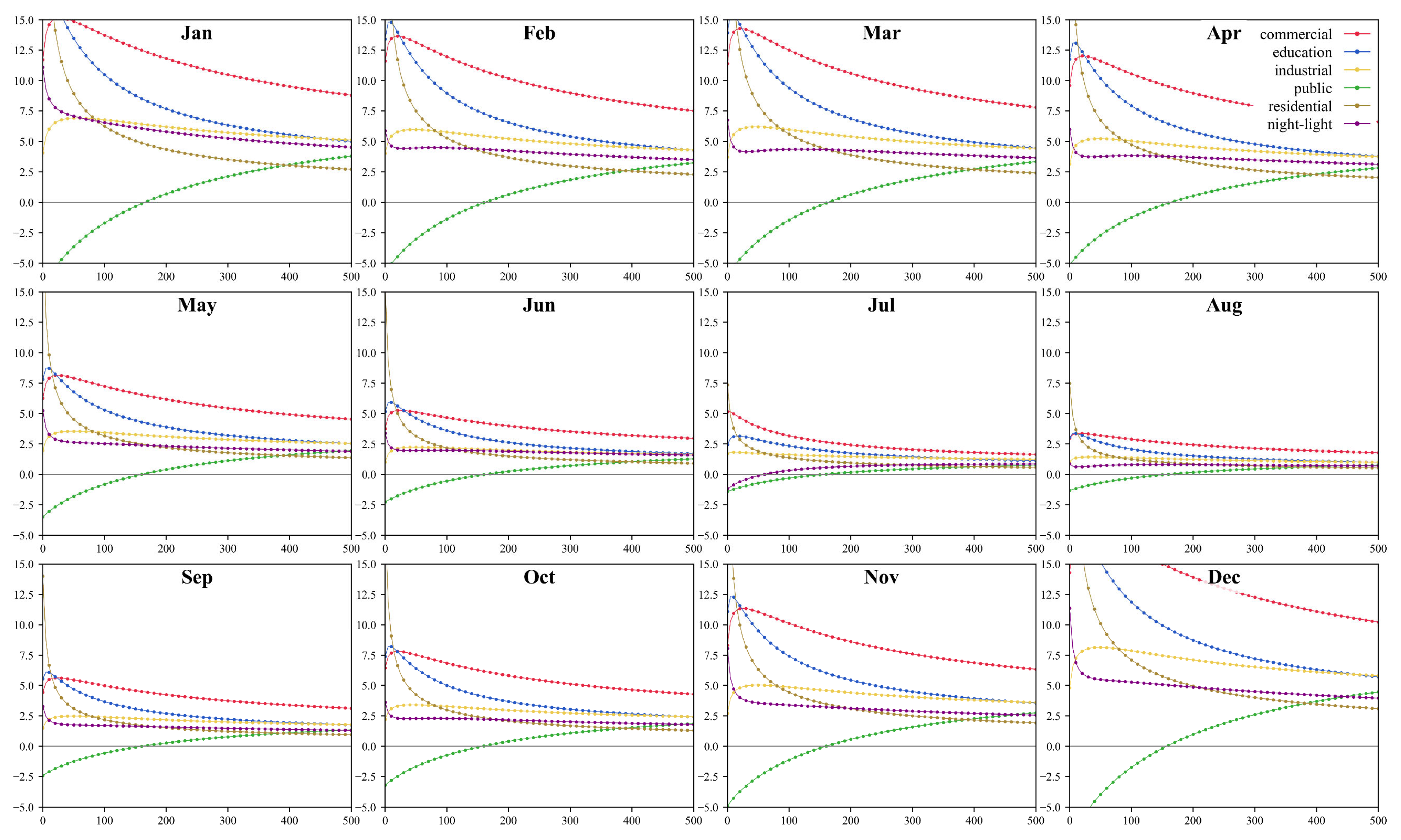
To select the optimal ridge regression penalty coefficient, we plotted monthly line charts for models 3 and 4 (defined in Section 2.4) to observe how the independent variables evolve as the penalty coefficient gradually increases. As shown in Figure 7, the coefficient trajectories for model 4 based on scaled predictors were plotted across a range of α values, with steps of 10, around the point where all coefficients approached zero. It can be observed that as the penalty term increases, the coefficient curves shift from divergence to convergence, with each predictor’s coefficient gradually stabilizing and becoming flatter. Notably, the upward trend in the public building curve may stem from its broad definition, suggesting that this variable captures unique predictive information orthogonal to others. To obtain the accurate optimal α value, we employed leave-one-out cross-validation. The results revealed that the optimal α varied across different months. When α was set to 170, all predictor coefficients in model 4 remained positive for each month, and this value achieved the maximum R² and minimum RMSE, thereby avoiding model underfitting. By analogy, the optimal α for model 3 was calculated to be 145. Accordingly, we set the final α values for models 3 and 4 at 145 and 170, respectively, for subsequent evaluation of the regression equations.

Figure 7. Monthly line charts of the coefficient of the independent variables varying with α, where the x-axis represents the penalty coefficient α, and the y-axis represents the magnitude of the coefficients.

3.1.1. Comparison of Performance Among Different Models

Table 3 presents the training set statistical performance metrics for the four models. For model 1, the average R² and adjusted R² per month are 0.877 and 0.874, respectively, with RMSE ranging from 15,590 to 88,320 tons. For model 2, the average R² is 0.936, and the average adjusted R² is 0.934, with RMSE ranging from 11,900 to 67,960 tons. Models 3 and 4 exhibit average R² values of 0.953 and 0.951, and adjusted R² values of 0.946 and 0.943, with average RMSE values of 31,707 tons and 32,086 tons, respectively. RMSE for all models generally decreases from January, reaches its lowest point in August, and then gradually increases, peaking in December. This may be because all models learned the temporal pattern of stable low emissions in summer versus higher emissions in winter due to heating demand.

Table 3. Comparison of statistical metrics for models 1–4.

Month	Model 1			Model 2			Model 3			Model 4
	Night Light (NL)			NL + Unclassified BV			Building Volume (BV)			NL + BV
	R2	Adjusted R2	RMSE (104 tons)	R2	Adjusted R2	RMSE (104 tons)	R2	Adjusted R2	RMSE (104 tons)	R2	Adjusted R2	RMSE (104 tons)
Jan	0.902	0.900	7.446	0.936	0.934	6.071	0.953	0.946	5.171	0.953	0.945	5.180
Feb	0.896	0.893	6.469	0.936	0.934	5.125	0.953	0.946	4.366	0.952	0.944	4.414
Mar	0.891	0.888	6.901	0.936	0.934	5.340	0.953	0.946	4.549	0.952	0.943	4.608
Apr	0.896	0.894	5.703	0.936	0.934	4.523	0.953	0.946	3.853	0.952	0.944	3.900
May	0.902	0.900	3.728	0.936	0.934	3.036	0.953	0.946	2.586	0.952	0.943	2.618
Jun	0.902	0.900	2.521	0.936	0.934	2.060	0.953	0.946	1.755	0.952	0.944	1.767
Jul	0.680	0.672	2.933	0.936	0.934	1.320	0.953	0.946	1.124	0.949	0.941	1.166
Aug	0.888	0.885	1.559	0.936	0.934	1.190	0.953	0.946	1.014	0.951	0.943	1.032
Sep	0.897	0.894	2.637	0.936	0.934	2.097	0.953	0.946	1.787	0.951	0.943	1.811
Oct	0.892	0.889	3.695	0.936	0.934	2.872	0.953	0.946	2.447	0.951	0.943	2.480
Nov	0.893	0.890	5.421	0.936	0.934	4.234	0.953	0.946	3.607	0.951	0.943	3.656
Dec	0.890	0.887	8.832	0.936	0.934	6.796	0.953	0.946	5.789	0.951	0.943	5.871

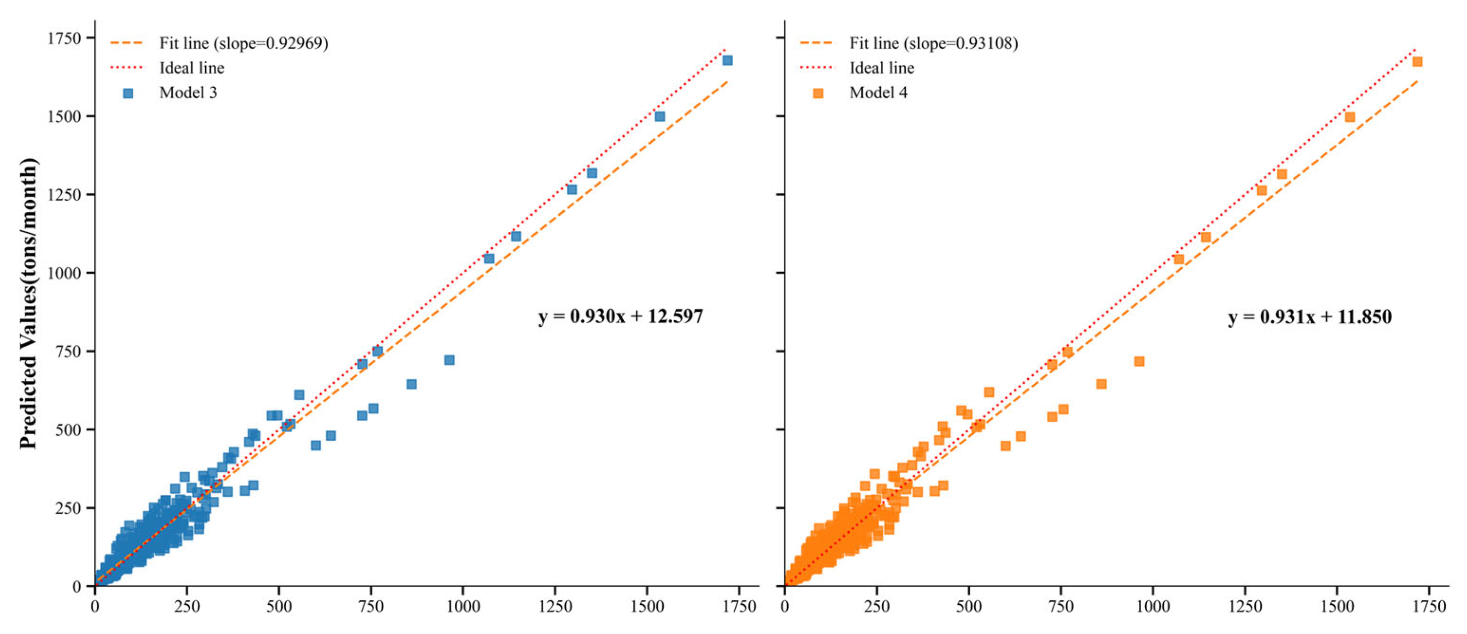
We found that model 1, which was based solely on building volume data, performed the worst. Model 2, which incorporated building volume and night-time lights as independent variables, exhibited relatively low fitting accuracy and its root mean square error (RMSE) was higher than that of models 3 and 4, indicating that it did not achieve satisfactory fitting performance. In contrast, models 3 and 4 both demonstrated superior generalization capabilities. To further evaluate the models’ effectiveness and assess their performance in allocating carbon emissions from different functional buildings, we plotted scatterplots comparing the true versus predicted carbon emissions of each spatial unit for models 3 and 4 (Figure 8).

Figure 8. Scatterplots of true and predicted CO₂ emissions for model 3 and model 4. Each point represents the CO₂ emissions of a spatial unit for a given month, with each scatterplot containing 528 points (44 spatial units multiplied by 12 months).

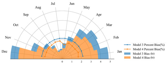
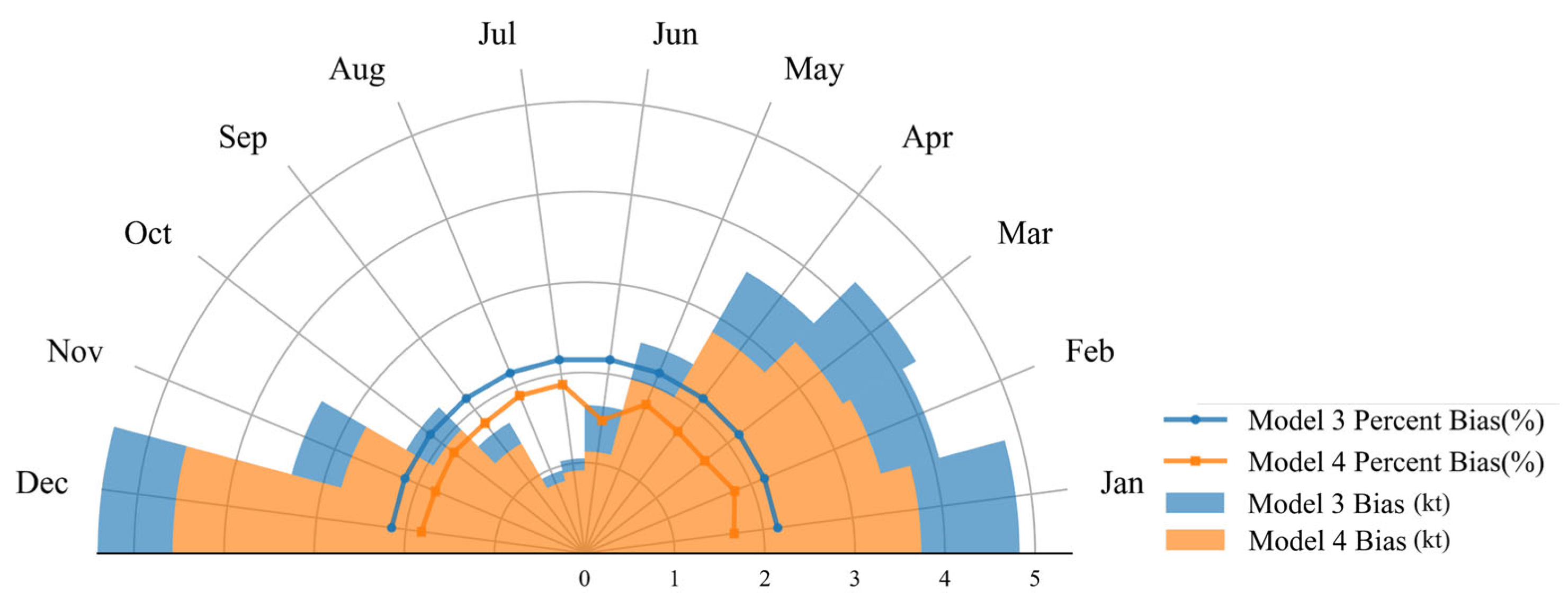
As shown in Figure 8, model 4 demonstrated relatively superior unbiasedness. The slopes of the fitted curves for model 3 and model 4 deviate from 1 to a similar extent, with little difference between them, while the intercept of the fitted curve for model 4 was smaller, suggesting that model 4 yielded smaller errors when predicting building CO₂ emissions monthly in each unit, thus reducing systematic overestimation or underestimation of building CO₂ emissions. To more explicitly illustrate the presence of data bias in the model predictions, a stacked radar chart comprising monthly mean residuals and percent bias for model 3 and model 4 was constructed. As shown in Figure 9, both models exhibited the largest prediction bias in December, which gradually decreased and reached a minimum during July and August, followed by an increase thereafter. This suggests that higher actual carbon emissions are associated with greater prediction bias. Notably, model 4 consistently produced smaller monthly mean residuals than model 3. In addition, the line plots reveal that model 4 maintained a relatively low percent bias across all months, demonstrating superior stability in carbon emission allocation performance.

Figure 9. The filled sectors in the radar chart represent the monthly mean residuals of the models, with each month occupying a 15-degree segment, and the overlaid line plots represent the percent bias of the predicted values.

In summary, model 4 had higher R² and adjusted R², as well as lower RMSE, compared to model 1 and model 2, indicating superior performance. Moreover, the inclusion of night-time lights as an additional independent variable helped to better mitigate the underestimation or overestimation of systemic building carbon emissions compared to model 3, particularly in months with higher carbon emissions. This suggests that incorporating both building volume and night-time lighting (six independent variables) enhanced the model’s explanatory power, providing a more realistic representation by integrating all types of building volumes and night-time light data. Therefore, model 4 proved to be the most reliable and reasonable model for exploring the patterns of CO₂ emissions through building classification.

3.1.2. Model Coefficient Analysis

The coefficients of model 4 are presented in Table 4. From the model coefficients, we found that the coefficient values of all independent variables gradually decreased starting in January, reaching their lowest in July or August. Afterward, all coefficients increased again, peaking in December. This trend suggested that the impact of changes in building volume and night-time lighting on CO₂ emissions during the winter months was significantly greater than that during summer. Furthermore, commercial buildings had the highest coefficients among the same coefficient type a_ij, indicating that commercial buildings contribute the most CO₂ emissions per unit volume. Educational and industrial buildings followed, with public buildings ranking next, and residential buildings contributed the least CO₂/volume ratio. Meanwhile, the average CO₂ emissions per unit volume in commercial buildings, calculated based on Table 4, were approximately 26 times higher than those in residential buildings in 2022. Additionally, the F-test for each month were all statistically significant (p < 0.01), indicating that the predictive capability of the established model equations for building CO₂ emissions is statistically significant across all months. Based on the coefficients obtained from model 4, we used Equation (11) to disaggregate building CO₂ emission data for individual buildings in England from January to December.

$${\mathrm{y}}_{\mathrm{i}\mathrm{j}}={\mathrm{a}}_{\mathrm{i}\mathrm{j}}\ast {\mathrm{V}}_{\mathrm{j}}+{\mathrm{b}}_{\mathrm{i}}\ast {\mathrm{L}}_{\mathrm{i}\mathrm{j}}$$

(11)

where y_ij represents the CO₂ emissions of building j in month i; a_ij and b_i are the model coefficients for building type j and the night-time light variable, respectively, for month i; V_j is the volume of building j; and L_ij is the night-time light value of building j in month i.

Table 4. Monthly independent variable coefficients of model 4.

Month	Commercial	Education	Industrial	Public	Residential	Night Light	F	Sig.
	aij					bi
Jan	1.232	0.829	0.637	0.111	0.047	6.001	118.560	0.000
Feb	1.064	0.709	0.538	0.150	0.040	4.330	115.902	0.000
Mar	1.108	0.742	0.556	0.129	0.042	4.314	115.713	0.000
Apr	0.938	0.627	0.470	0.102	0.036	3.753	115.906	0.000
May	0.645	0.419	0.320	0.110	0.024	2.389	115.541	0.000
Jun	0.416	0.284	0.204	0.057	0.016	1.932	117.775	0.000
Jul	0.260	0.189	0.151	0.064	0.010	0.600	109.988	0.000
Aug	0.256	0.165	0.127	0.056	0.009	0.812	114.065	0.000
Sep	0.444	0.291	0.224	0.070	0.017	1.623	115.221	0.000
Oct	0.608	0.397	0.306	0.125	0.023	2.212	115.155	0.000
Nov	0.900	0.587	0.454	0.160	0.034	3.203	115.236	0.000
Dec	1.454	0.941	0.732	0.319	0.054	4.996	115.012	0.000

3.2. Spatial Analysis of the Results

3.2.1. National-Scale Building CO₂ Emissions Analysis

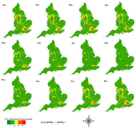
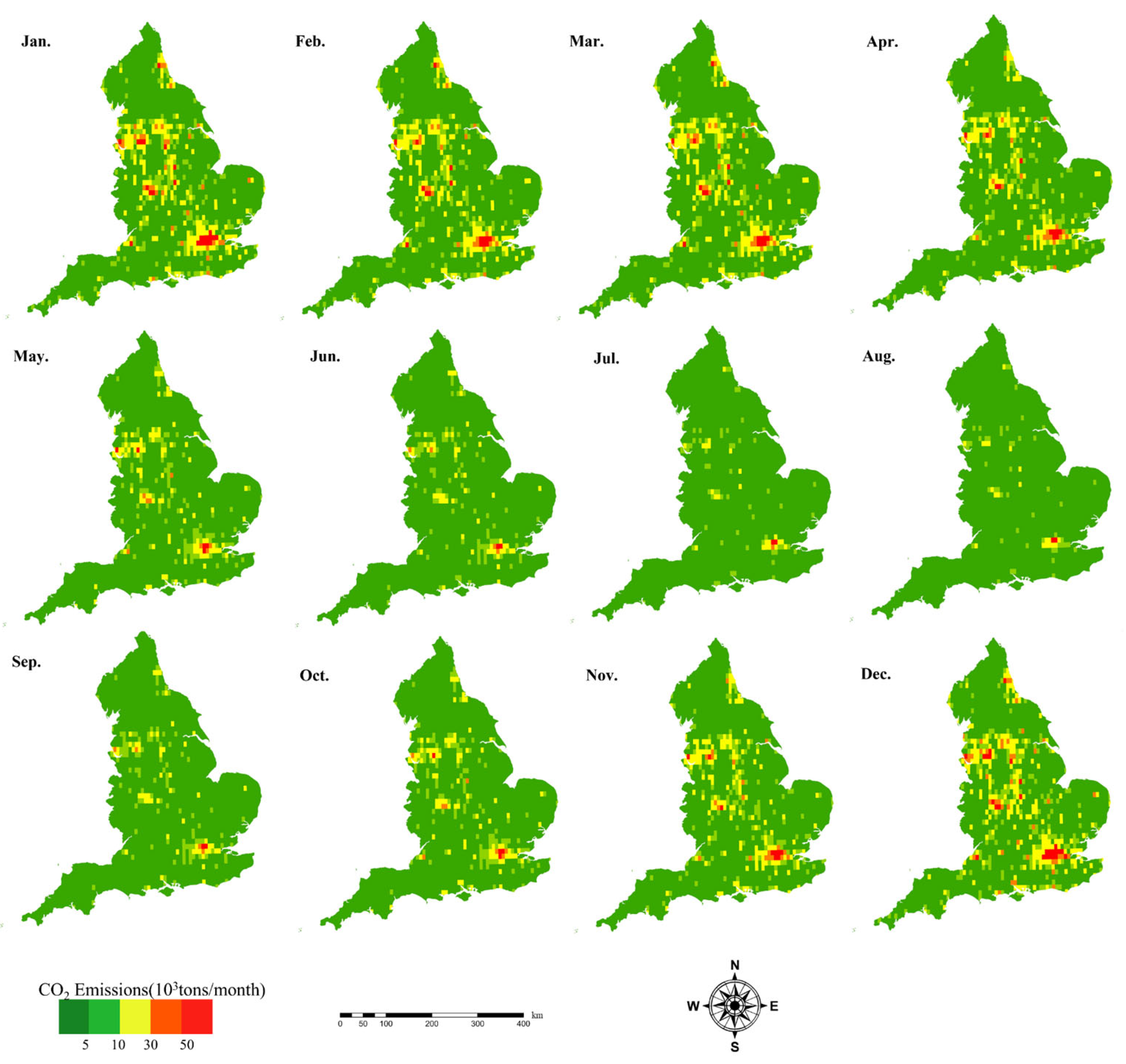
By calculating CO₂ emissions based on model formula and coefficients, we visualized the national distribution of building CO₂ emissions at a 0.1° × 0.1° grid scale (Figure 10) to observe their spatiotemporal changes more clearly. Spatially, only certain urban centers in specific regions exhibited persistent red-colored grids throughout the year, such as Greater London, parts of Yorkshire, the West Midlands, and Manchester, where grid CO₂ emissions exceeded 50,000 tons/month and many individual buildings exceeded 20 tons/month. In contrast, most other regions demonstrated significantly lower emissions, with grid CO₂ emissions typically below 5000 tons/month and almost all individual building emissions predominantly under 1 ton/month.

Figure 10. Gid-scale CO₂ emissions from buildings in England from January to December.

From the perspective of temporal changes, CO₂ emissions from buildings exhibited seasonal variability, with significantly lower emissions in summer compared to winter. During the summer, the majority of regions demonstrated relatively low and balanced carbon emissions, with only sporadic red or orange grid cells observed in a few urban centers, indicating grid CO₂ emissions exceeding 30,000 tons/month. These high-emission grid cells contained numerous individual buildings with monthly emissions exceeded 10 tons/month. However, in winter, the number of red buildings increased substantially, particularly in January and December. There was a high and relatively uniform distribution of red buildings across the country, likely due to the increased energy demand for building heating during the colder months.

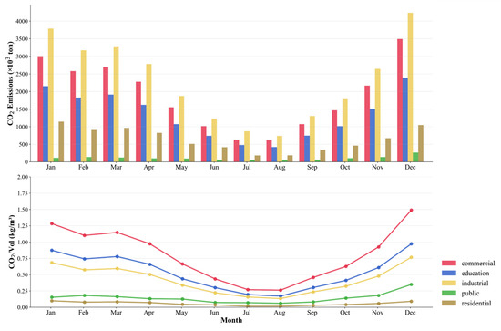
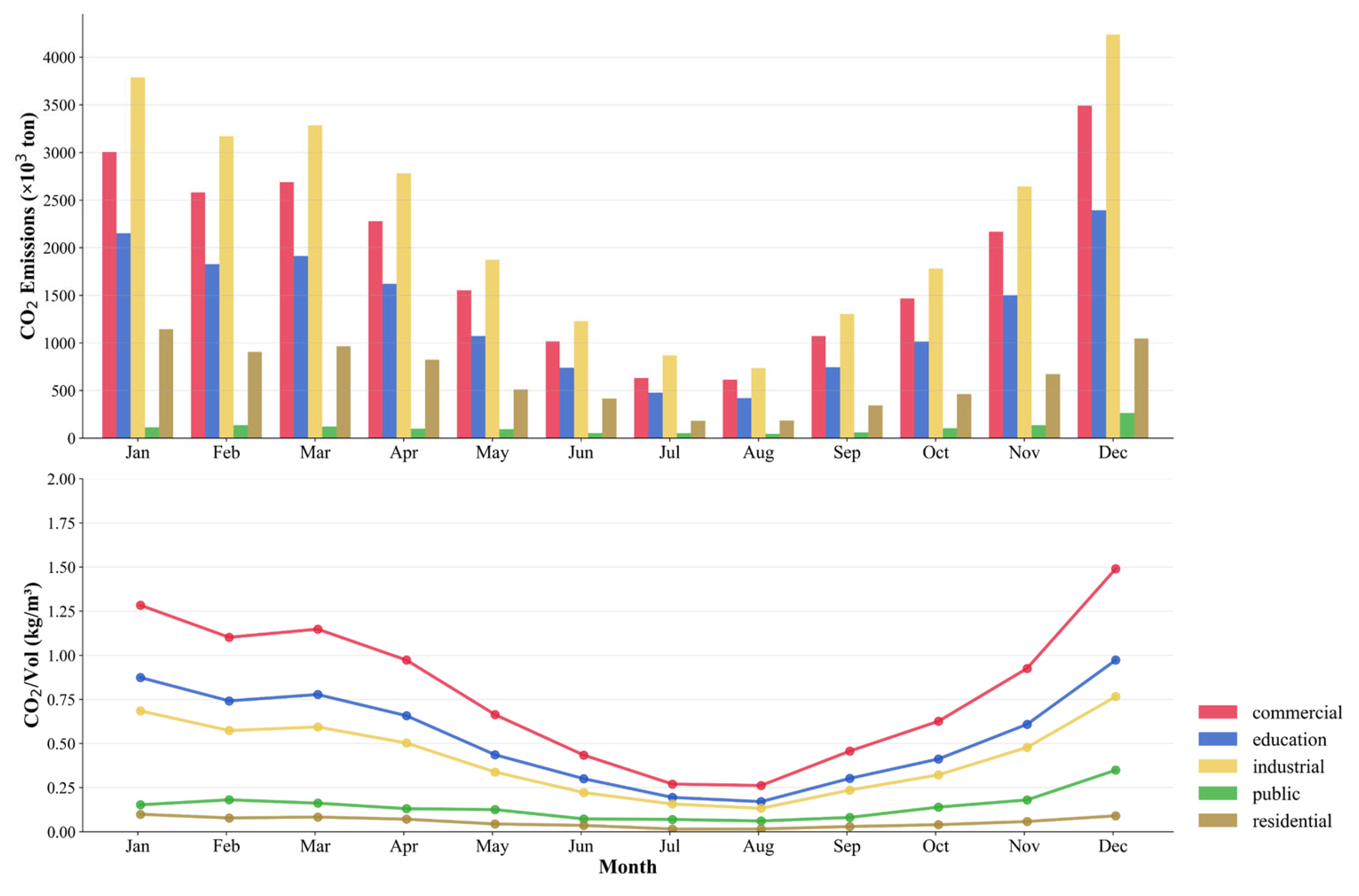
To further evaluate building CO₂ emissions from different functional buildings, we also plotted graphs of monthly CO₂ emissions and monthly CO₂/Vol ratios for all functional buildings, as shown in Figure 11. The graph highlights the CO₂ emission efficiency of different functional buildings each month. The analysis revealed significant variations in CO₂ emissions, which may be attributed to inconsistent energy consumption from different functional buildings driven by varying activity levels. Industrial buildings had the highest total CO₂ emissions, with 736.362 tons in August and 4238.138 tons in December. Commercial, educational, residential, and public buildings followed. Public buildings had the lowest emissions, at 46.341 tons in August and 263.854 tons in December, meaning that industrial buildings’ average monthly CO₂ emissions were approximately 21.5 times those of residential buildings. Furthermore, commercial buildings had the highest CO₂/Vol ratio, with a ratio of 1.490 kg/m³ in December, which is 5.51 and 5.68 times higher than in July and August, respectively. Educational, industrial, and public buildings followed, while residential buildings had the lowest CO₂/Vol ratio, which did not exceed 0.25 kg/m³ even at its peak in December. It should be noted that although industrial buildings have the highest total CO₂ emissions, their CO₂/Vol ratio is lower than that of commercial buildings. This may be attributed to the large volume and dense distribution of industrial buildings, resulting in high total CO₂ emissions. In contrast, commercial buildings had higher energy consumption and CO₂/Vol ratio due to the intensive use of systems such as air conditioning, lighting, and elevators.

Figure 11. The bar chart represents the monthly CO₂ emissions of each building functional type, and the line chart depicts the monthly CO₂/Vol for each building functional type.

3.2.2. County-Scale Building CO₂ Emissions Analysis

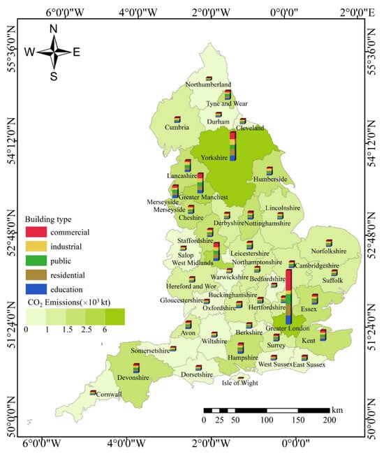
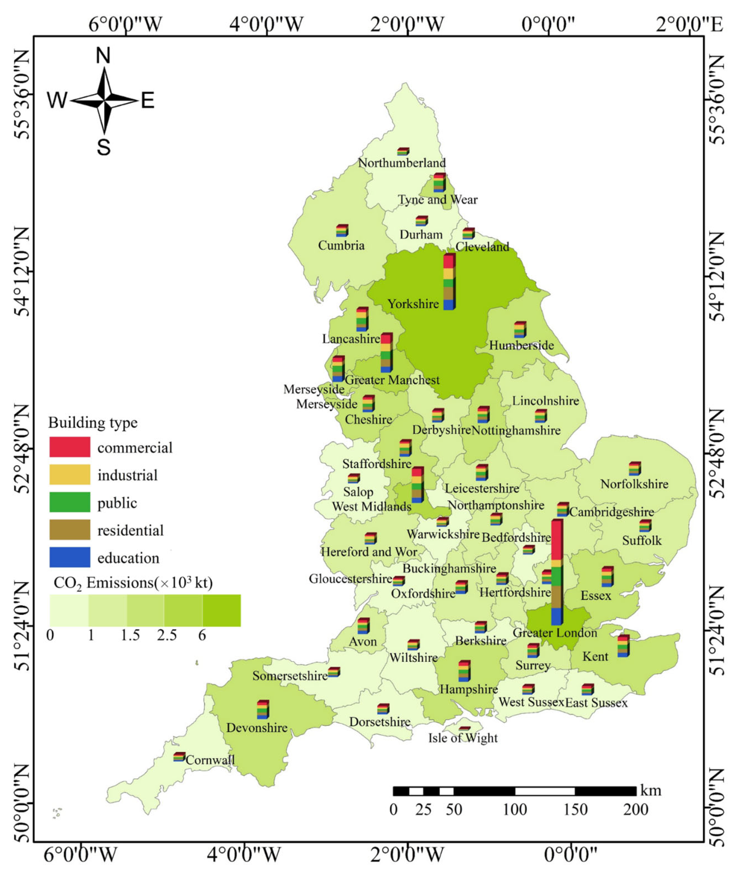
We further visualized the annual total CO₂ emissions of different functional buildings in each county using stacked bar charts (Figure 12). Spatially, it is obvious that London, Yorkshire, the West Midlands, and Greater Manchester exhibited significantly higher CO₂ emissions compared to other regions, while emissions in most other counties were generally below 1500 kilotons. Notably, the combined CO₂ emissions from industrial and commercial buildings accounted for more than half of the regional total CO₂ emissions, averaging 65.95%, followed by residential and educational buildings. Public buildings had the lowest total CO₂ emissions, averaging 9.99%. These indicated that industrial and commercial buildings were the primary contributors to CO₂ emissions from buildings, which was likely due to the high energy dependence and relatively lower operational efficiency of industrial buildings, as well as the significant energy consumption in commercial buildings.

Figure 12. Total annual CO₂ emissions from different functional buildings in each county.

From a spatial distribution perspective, counties with higher CO₂ emissions were mainly located in southeastern England (especially the Greater London area), and certain northern regions (such as industrial city belts, including the West Midlands, Greater Manchester, and Merseyside). Furthermore, the relatively high CO₂ emissions in Yorkshire may be attributed to a combination of its large area, dense and widespread building stock, and particularly the slow renovation of aging industrial facilities. It is worth noting that Greater London’s commercial buildings accounted for 56.7% of the region’s total CO₂ emissions, which may be explained by the dominance of finance and technology industries in the area. Similarly, in the West Midlands, industrial and commercial building emissions constituted 32.45% and 37.43%, respectively, which was known for its manufacturing and service sectors.

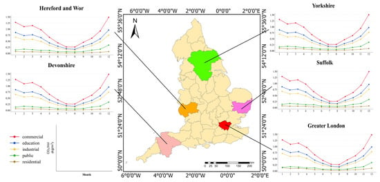
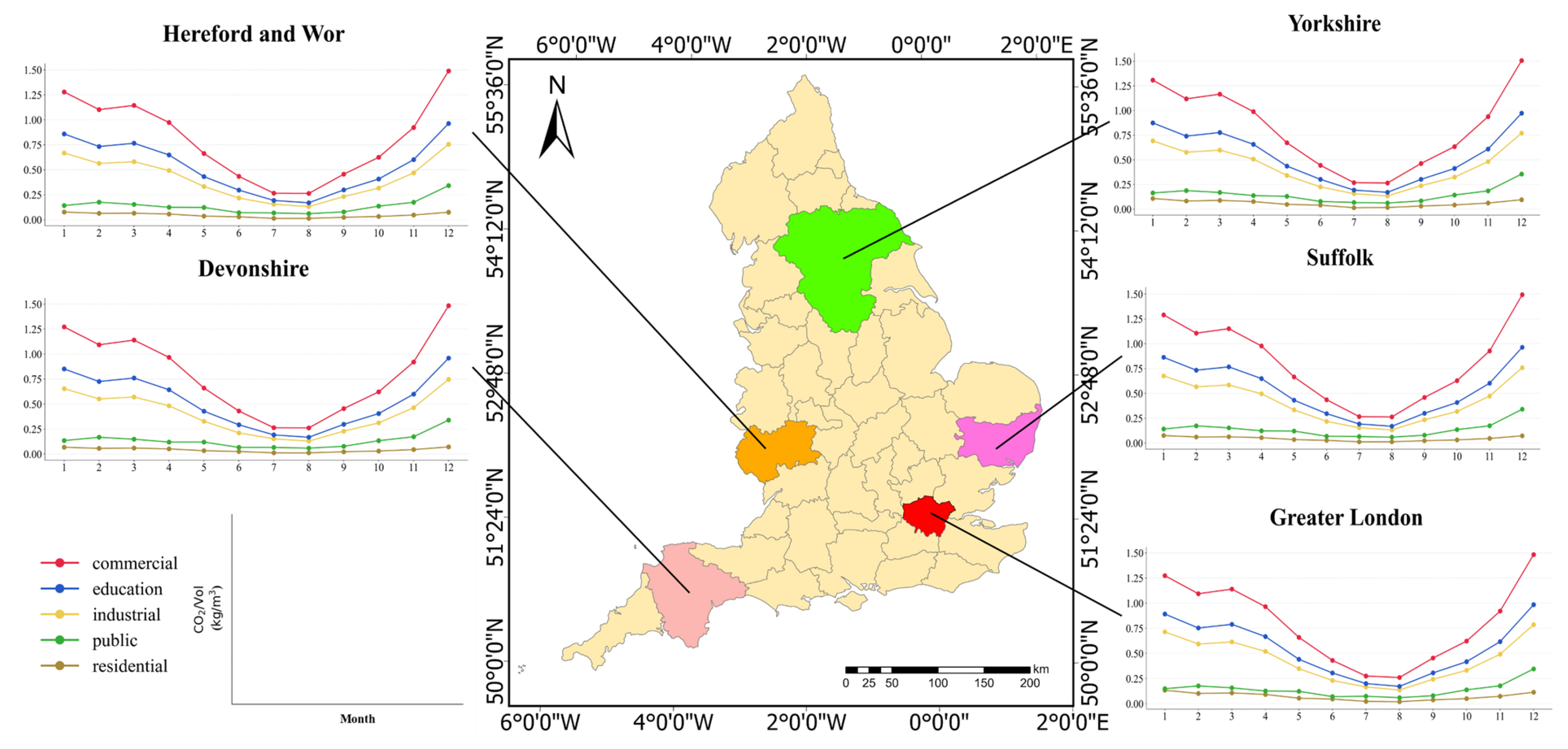
We also selected five counties and plotted corresponding line graphs based on the CO₂/Vol ratio for each county to observe changes in CO₂ emissions from buildings over time (Figure 13). We found that for all buildings in each county, the CO₂/Vol ratio decreased from January to July, reached its lowest point in August, and then increased gradually from September to December, forming a ‘V’ shape. Furthermore, there were differences in the CO₂/Vol ratio among the same functional buildings across different regions. As the capital of the UK, the CO₂/Vol ratio of commercial buildings in Greater London was comparable to that in other regions. However, the CO₂/Vol ratio for educational, industrial, public, and residential buildings were relatively higher in Greater London compared to other regions, with residential buildings in London having nearly double the CO₂/Vol ratio of Devonshire. This discrepancy may be attributed to lower vacancy rates of commercial buildings in Greater London, especially at night. Consequently, despite similar CO₂/Vol ratio, London’s total emissions were higher due to longer periods of usage.

Figure 13. Monthly CO₂/Vol ratio of different functional buildings in five selected counties.

To better illustrate differences in CO₂ emissions across counties, we also plotted a table displaying the average CO₂ emissions of each county, where the average CO₂ emissions refer to the average amount of CO₂ emitted by a single building per month (Table 5, Com, Edu, Ind, Pub, and Res are the abbreviations for commercial, education, industrial, public, and residential). We found that economically developed regions generally had higher total CO₂ emissions and higher average CO₂ emissions of various building functions, which indicated regional disparities in CO₂ emissions. For example, Greater London, Manchester, the West Midlands and York exhibited particularly high monthly average CO₂ emissions from commercial, educational and industrial buildings. Furthermore, the monthly average CO₂ emissions of public and residential buildings showed relatively stable variations across most counties. Only public buildings in a few counties and residential buildings in a very small number of counties had monthly CO₂ emissions exceeding 1 ton. This may be attributed to similar usage patterns and more uniform energy consumption standards for public and residential buildings, resulting in smaller differences. Regions with higher monthly average CO₂ emissions from public and residential buildings likely had higher population densities and more permanent residents.

Table 5. Average CO₂ emissions of all functional buildings in each county.

Ave CO2 (ton/m3)	Com	Edu	Ind	Pub	Res	Ave CO2 (ton/m3)	Com	Edu	Ind	Pub	Res
Avon	8.035	4.663	3.069	1.582	0.066	Isle of Wight	7.522	3.863	1.700	0.715	0.041
Bedford	9.549	3.503	3.613	0.607	0.061	Kent	7.656	3.151	2.935	0.426	0.052
Berk	10.186	4.614	3.340	0.691	0.057	Lanca	8.230	4.068	2.967	0.632	0.054
Buckingham	10.376	3.687	2.573	0.543	0.056	Leicester	8.238	3.855	3.802	0.577	0.053
Cambridge	7.820	3.794	2.935	0.785	0.051	Lincoln	4.820	2.362	2.335	0.353	0.038
Che	7.269	3.862	4.155	1.144	0.053	Mersey	7.653	5.636	7.646	1.629	0.095
Cleveland	12.354	5.140	6.975	1.403	0.075	Norfolk	6.310	2.871	1.904	0.389	0.043
Cornwall	4.595	2.406	1.378	0.324	0.035	Northampton	10.155	3.154	4.934	0.619	0.054
Cumbria	5.968	5.971	2.814	0.383	0.044	Northumberland	7.497	4.170	2.615	0.838	0.054
Derby	5.515	3.657	3.332	0.445	0.051	Nottingham	7.238	5.242	4.030	0.925	0.062
Devon	7.104	3.279	1.827	0.386	0.043	Oxford	9.813	4.682	2.961	0.824	0.054
Dorset	7.300	3.524	1.890	0.400	0.042	Salop	7.350	3.386	2.591	0.344	0.041
Durham	7.370	4.133	3.912	0.609	0.063	Somerset	7.299	2.836	1.756	0.360	0.042
East Sussex	9.784	3.911	1.572	0.479	0.050	Stafford	9.585	4.621	3.460	0.819	0.059
Essex	6.555	3.633	2.074	0.552	0.054	Suffolk	6.016	2.933	2.625	0.367	0.042
Gloucester	6.622	3.142	2.470	0.544	0.044	Surrey	9.772	3.126	1.827	0.570	0.048
Greater London	22.240	7.444	6.424	3.103	0.173	Tyne and Wear	15.907	9.338	8.278	1.958	0.114
Greater Manchester	12.494	6.007	5.755	1.758	0.080	Warwick	11.396	4.510	3.561	0.675	0.058
Hamp	7.623	4.041	2.668	0.737	0.051	West Midlands	17.760	8.931	8.247	4.792	0.109
Hereford and Worcester	8.312	3.212	1.838	0.377	0.045	West Sussex	11.050	4.000	1.527	0.484	0.049
Hertford	10.122	4.284	3.462	0.688	0.061	Wilt	5.944	3.183	2.317	0.449	0.046
Humberside	8.613	4.153	4.332	0.680	0.055	York	11.011	5.418	4.103	0.606	0.064

We also found that, possibly due to variations in industrial structure across regions, some counties exhibited low total CO₂ emissions while maintaining high average monthly CO₂ emissions for specific building functional types, exhibiting a “high average–low total” pattern. For example, although the Isle of Wight had the lowest total CO₂ emissions, it showed relatively high average monthly emissions from commercial and public buildings. This may be attributed to the island’s tourism-driven economy, which stimulates the development of commerce and public services, thereby increasing average emissions. Notably, Greater London exhibited significantly higher average CO₂ emissions from all functional buildings compared to other regions. In particular, the average emissions from commercial buildings in Greater London were markedly higher, likely due to the presence of large-scale commercial structures, including skyscrapers and expansive commercial complexes, which contributed substantially to the regional average.

3.2.3. Building-Scale Building CO₂ Emissions Analysis

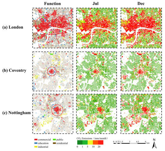
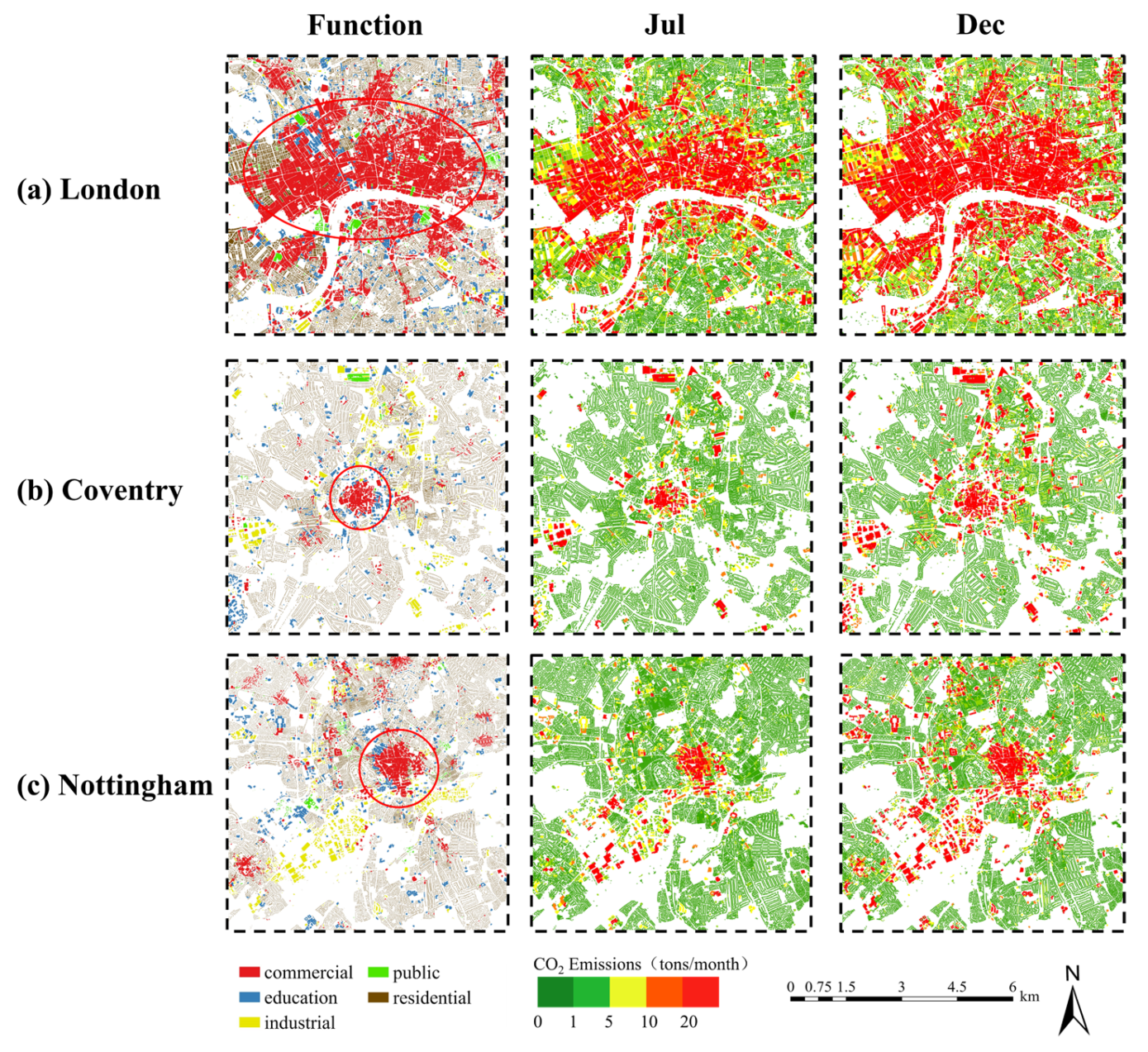
We selected the central urban areas of three counties in England and conducted a comparative analysis of CO₂ emissions at the building scale for both summer and winter, using July and December as examples (Figure 14).

Figure 14. Building classification results, CO₂ emissions from buildings in July and CO₂ emissions from buildings in December for the three selected counties.

(i) London: London, located in the southeastern corner of the UK, is the capital city and plays a central role in politics, economy, culture, and transportation. This county features a relatively dense and large-scale cluster of buildings, predominantly commercial structures. As shown in Figure 14a, during July, commercial buildings exhibited higher CO₂ emissions, particularly in the central area north of the River Thames, where emissions generally exceeded 10 tons/month. By December, CO₂ emissions from all buildings increased significantly, with some mixed-use commercial complexes emitting over a thousand tons per month. This showed a notable increase from summer to winter. Furthermore, it is evident that central London contains extensive clusters of buildings with high CO₂ emissions, with commercial, industrial, educational, public, and residential buildings all exceeding 10 tons of CO₂ emissions per month.

(ii) Coventry: Coventry, located in the heart of the UK, is a prominent city in England known for its manufacturing base—most notably the automotive industry. As shown in Figure 14b, the city contained a high concentration of industrial structures, particularly in its southwest and northeast zones. Although Coventry’s overall CO₂ emissions were relatively low, commercial and industrial buildings exhibited high CO₂ emissions throughout the year, especially in the city center and northeastern areas. Educational buildings were more diffusely distributed and exhibited moderate CO₂ emissions, and other building types had very low emissions. Owing to the predominance of industrial and commercial use, these two types together accounted for the bulk of the city’s total CO₂ emissions. Moreover, from July to December, the average percentage increase in CO₂ emissions from buildings in Coventry was lower than that in London.

(iii) Nottingham: Nottingham, located in the East Midlands of the UK, is celebrated for its historical landmarks and academic institutions, notably the University of Nottingham and Nottingham Trent University. As shown in Figure 14c, there was significant spatial heterogeneity in CO₂ emissions from buildings in July. Most commercial buildings, along with some industrial and educational buildings, exhibited high CO₂ emissions, whereas public and residential buildings typically remain low. By December, the CO₂ emissions of many educational buildings and several smaller commercial and industrial buildings showed marked emission increases, while CO₂ emissions from public and residential buildings remained generally under 5 tons per month. In contrast to London’s concentrated high-emission cores, Nottingham’s elevated-emission buildings are more evenly dispersed.

The CO₂ emissions from buildings across all three regions shared several common characteristics. Spatially, CO₂ emissions conformed to a power-law distribution: urban cores, predominantly characterized by commercial activities, exhibited the highest levels, which gradually diminished toward the peripheral zones. Furthermore, marked variations also emerged by building function, with commercial and industrial buildings exhibiting the highest emissions, followed by educational buildings. In contrast, public and residential buildings remained relatively low in emissions, appearing as more uniform green areas in the figures. In terms of temporal changes, CO₂ emissions exhibited pronounced seasonality, with emissions in winter being higher for nearly every building type compared to summer.

3.3. Research Limitations

It should be noted that, since the framework depends heavily on EDGAR data, the quality of the EDGAR data inevitably influences the reliability of the resulting spatial patterns. The downscaling process employed in this study relies on a series of strong assumptions, which may give rise to the Modifiable Areal Unit Problem (MAUP) and introduce uncertainties during scale transformation. Secondly, only two factors (night-time lights and building CO₂ emissions) were considered in this model, which may be incomplete, leading to underestimation of CO₂ emissions for specific building types and thus inaccurate results. Other potential influencing variables, such as economic data and population distribution, should be evaluated and incorporated. Furthermore, the building-level CO₂ emission data disaggregated by the model are difficult to verify. Comprehensive field surveys should be conducted to obtain stable and reliable real building CO₂ emission data. These data can then be used to corroborate the experimental results and assess the accuracy of the methodology. Therefore, it should be emphasized that the results of this paper represent model-based allocation rather than validated building-level estimates. In addition, the model used in this study inherently assumed that the same functional buildings share consistent energy consumption coefficients, which may overlook spatial heterogeneity among different regions. Future research could explore other appropriate downscaling methods to obtain more accurate building-level CO₂ emission data. Furthermore, many urban buildings have mixed functions in reality, so the single-function assumption may bias emission allocation toward the dominant function, thereby diluting emissions from ancillary uses.

Moreover, this study focused solely on CO₂ emission patterns of buildings in England in 2022. However, building CO₂ data and night-time light data for more recent years are available. Collecting time series data and applying this method to assess long-term trends in building CO₂ emission should be feasible. With continuous updates of more accurate building vector data, it should also be straightforward to extend this method to other regions, enabling broader applications.

4. Policy Implications

With the advancement of greenhouse gas reduction and sustainable development goals, it has become critically important to reduce building CO₂ emissions and to formulate regulations and policies tailored to the characteristics of different building types. The method proposed in this study constructs a building classification model and integrates readily accessible datasets—gridded monthly CO₂ emissions and night-time light—to develop a ridge regression model for disaggregating CO₂ emissions at the building scale. This approach has been demonstrated as an effective method to rapidly obtain building-level CO₂ emissions across large regions. The findings may not only enrich the literature on the relationship between buildings and CO₂ emissions but also provide feasible and effective support for promoting urban CO₂ reduction.

The research revealed that variations in building functions significantly impact energy consumption distribution, leading to considerable differences in CO₂ emissions. To more effectively control CO₂ emissions, differentiated standards for CO₂ emissions should be established for different functional buildings. For example, commercial buildings in England typically have prolonged operations and intensive commercial activities, resulting in relatively high total operational CO₂ emissions as well as substantially higher CO₂ emission intensity per unit volume. Measures such as enhancing operational energy efficiency, reinforcing refined energy management, and setting stringent energy consumption caps may be effective. Furthermore, rational urban functional zoning can play an important role in carbon mitigation. Scientifically planned building clusters and more coordinated spatial arrangements of different functional buildings can help reduce operational burdens arising from functional mismatches. In conclusion, policymakers should establish suitable urban functional area layouts and pay attention to the CO₂ emission characteristics of different building functions to implement differentiated policies, which may more effectively contribute to reducing CO₂ emissions from buildings.

5. Conclusions

In this study, we combined building volume data, EDGAR CO₂ emission grid maps, and NPP-VIIRS night-time light images to allocate monthly CO₂ emissions based on building classifications through ridge regression analysis. Our proposed model achieved an R² of 0.951 and an adjusted R² of 0.943, demonstrating its effectiveness and reliability. The analysis of nearly 11.5 million buildings in England revealed that industrial buildings had the highest total emissions, while commercial buildings exhibited the highest CO₂ intensity (1.49 kg/m³ in February). Emissions peaked in winter across all building types, highlighting that both functional differences and seasonal energy demand drive the spatial and temporal heterogeneity of urban CO₂ emissions.

In summary, the method proposed in this paper fills the gap in obtaining spatiotemporal distribution data of CO₂ emissions from different functional buildings across large regions. It is important to note that detailed CO₂ emissions data from different functional buildings are expected to become a crucial input for sustainable development, such as carbon footprint accounting and policy-making for functional zoning. Due to continuous updates of high-precision global building vector datasets, our proposed method for quickly, simply, and cost-effectively acquiring CO₂ emissions data for large regions from different functional buildings has significant potential. Furthermore, our method allocates totals based on a model, which introduces inherent and unavoidable uncertainty. Our future efforts aim to reduce this uncertainty, improve accuracy, consider more influencing factors, and test it to evaluate long-term building-level CO₂ emissions.

References

- He, H.; Kramer, R.J.; Soden, B.J.; Jeevanjee, N. State dependence of CO2 forcing and its implications for climate sensitivity. Science 2023, 382, 1051–1056. [Google Scholar] [CrossRef] [Scilit] [PubMed]
- World Resources Institute. Our Top Articles 2024. WRI Insights. Available online: https://www.wri.org/insights/our-top-articles-2024 (accessed on 20 April 2025).
- Weiskopf, S.R.; Rubenstein, M.A.; Crozier, L.G.; Gaichas, S.; Griffis, R.; Halofsky, J.E.; Hyde, K.J.; Morelli, T.L.; Morisette, J.T.; Muñoz, R.C.; et al. Climate change effects on biodiversity, ecosystems, ecosystem services, and natural resource management in the United States. Sci. Total Environ. 2020, 733, 137782. [Google Scholar] [CrossRef] [Scilit] [PubMed]
- Khan, S.A.; Alam, T.; Khan, M.S.; Blecich, P.; Kamal, M.A.; Gupta, N.K.; Yadav, A.S. Life cycle assessment of embodied carbon in buildings: Background, approaches and advancements. Buildings 2022, 12, 1944. [Google Scholar] [CrossRef] [Scilit]
- Wang, G.; Luo, T.; Luo, H.; Liu, R.; Liu, Y.; Liu, Z. A comprehensive review of building lifecycle carbon emissions and reduction approaches. City Built Environ. 2024, 2, 12. [Google Scholar] [CrossRef] [Scilit]
- Benke, B.; Chafart, M.; Shen, Y.; Ashtiani, M.; Carlisle, S.; Simonen, K. A harmonized dataset of high-resolution embodied life cycle assessment results for buildings in North America. Sci. Data 2025, 12, 1085. [Google Scholar] [CrossRef] [Scilit] [PubMed]
- Fan, F.; Zhu, S.; Huang, J.; Xu, X.; Xu, F. Life cycle assessment of carbon emissions and reduction potential exploration of new building complexes in universities: A case study in China. Int. J. Life Cycle Assess. 2025, 30, 621–637. [Google Scholar] [CrossRef] [Scilit]
- Seyedabadi, M.R.; Karrabi, M.; Shariati, M.; Karimi, S.; Maghrebi, M.; Eicker, U. Global building life cycle assessment: Comparative study of steel and concrete frames across European Union, USA, Canada, and Australia building codes. Energy Build. 2024, 304, 113875. [Google Scholar] [CrossRef] [Scilit]
- CORDIS. One Click LCA—Transforming the Construction Industry Through Automated, Affordable and Scalable Solution for Assessing and Improving the Environmental Impacts of Construction Projects and Products. Available online: https://cordis.europa.eu/project/id/711303 (accessed on 20 April 2025).
- Zhang, H.; Cai, J.; Braun, J.E. A whole building life-cycle assessment methodology and its application for carbon footprint analysis of U.S. commercial buildings. J. Build. Perform. Simul. 2023, 16, 38–56. [Google Scholar] [CrossRef] [Scilit]
- Huang, W.; Xu, Q. Sustainable-driven renovation of existing residential buildings in China: A systematic exploration based on review and solution approaches. Sustainability 2024, 16, 3895. [Google Scholar] [CrossRef] [Scilit]
- Luo, C.; Yao, X.; Zhang, Y.; Zhou, H. An empirical study on the impact of different structural systems on CO2 emissions of prefabricated buildings based on SimaPro. World J. Eng. Technol. 2023, 11, 434–453. [Google Scholar] [CrossRef]
- Liu, G.; Zheng, Y.; Xu, X.; Liu, X.; Zhang, H.; Ou, J. Fine-scale estimation of building operation carbon emissions: A case study of the Pearl River Delta urban agglomeration. Build. Simul. 2025, 18, 957–977. [Google Scholar] [CrossRef] [Scilit]
- Grygierek, K.; Ferdyn-Grygierek, J.; Gumińska, A.; Baran, Ł.; Barwa, M.; Czerw, K.; Gowik, P.; Makselan, K.; Potyka, K.; Psikuta, A. Energy and environmental analysis of single-family houses located in Poland. Energies 2020, 13, 2740. [Google Scholar] [CrossRef] [Scilit]
- Liang, Y.; Li, C.; Liu, Z.; Wang, X.; Zeng, F.; Yuan, X.; Pan, Y. Decarbonization potentials of the embodied energy use and operational process in buildings: A review from the life-cycle perspective. Heliyon 2023, 9, e20190. [Google Scholar] [CrossRef] [Scilit] [PubMed]
- Gao, H.; Wang, X.; Wu, K.; Zheng, Y.; Wang, Q.; Shi, W.; He, M. A review of building carbon emission accounting and prediction models. Buildings 2023, 13, 1617. [Google Scholar] [CrossRef] [Scilit]
- Ke, Z.; Liu, X.; Zhang, H.; Jia, X.; Zeng, W.; Yan, J.; Hu, H.; Hien, W.N. Energy consumption and carbon emissions of nearly zero-energy buildings in hot summer and cold winter zones of China. Sustainability 2023, 15, 11453. [Google Scholar] [CrossRef] [Scilit]
- Wang, Y.; Guo, J.; Yue, Q.; Chen, W.Q.; Du, T.; Wang, H. Total CO2 emissions associated with buildings in 266 Chinese cities: Characteristics and influencing factors. Resour. Conserv. Recycl. 2022, 188, 106692. [Google Scholar] [CrossRef] [Scilit]
- Zhu, M.; James, P. Daily carbon assessment framework: Towards near real-time building carbon emission benchmarking for operative and design insights. Buildings 2022, 12, 1129. [Google Scholar] [CrossRef] [Scilit]
- Liang, H.; Zhang, B.; Qian, X.; Chen, Y.; Luo, Y.; Huang, Y.; Sun, L.; Zhou, C.; Long, J.; Dong, L. Building material stocks and embodied carbon dataset for two urban agglomerations in China from 2000 to 2020. Sci. Data 2025, 12, 930. [Google Scholar] [CrossRef] [Scilit]
- Hu, M.; Ghorbany, S. Building stock models for embodied carbon emissions—A review of a nascent field. Sustainability 2024, 16, 2089. [Google Scholar] [CrossRef] [Scilit]
- Zhao, Z.; Yang, X.; Yan, H.; Huang, Y.; Zhang, G.; Lin, T.; Ye, H. Downscaling building energy consumption CO2 emissions by machine learning. Remote Sens. 2021, 13, 4346. [Google Scholar] [CrossRef] [Scilit]
- Wang, T.; Sun, F. Global gridded GDP data set consistent with the shared socioeconomic pathways. Sci. Data 2022, 9, 221. [Google Scholar] [CrossRef] [Scilit] [PubMed]
- Xia, J.; Wang, J.; Lai, Y. Development strategy based on combination typologies of building CO2 emissions and urban vibrancy—A multi-sourced data-driven approach in Beijing, China. Land 2024, 13, 1062. [Google Scholar] [CrossRef] [Scilit]
- Rodríguez, R.L.; Duminil, E.; Ramos, S.J.; Eicker, U. Assessment of the photovoltaic potential at urban level based on 3D city models: A case study and new methodological approach. Sol. Energy 2017, 146, 264–275. [Google Scholar] [CrossRef] [Scilit]
- Guo, Z.; Wang, Q.; Zhao, N.; Dai, R. Carbon emissions from buildings based on a life cycle analysis: Carbon reduction measures and effects of green building standards in China. Low-Carbon Mater. Green Constr. 2023, 1, 9. [Google Scholar] [CrossRef] [Scilit]
- Mao, T.; Liu, Y.; Liu, Y.; Hao, M.; Chen, W. Towards sustainable building landscapes: A spatially explicit life-cycle analysis of carbon emissions and mitigation strategies. Landsc. Ecol. 2024, 39, 167. [Google Scholar] [CrossRef] [Scilit]
- Sun, Y. The impact of green buildings on CO2 emissions: Evidence from commercial and residential buildings. J. Clean. Prod. 2024, 469, 143168. [Google Scholar] [CrossRef] [Scilit]
- Yu, Y.; You, K.; Cai, W.; Feng, W.; Li, R.; Liu, Q.; Chen, L.; Liu, Y. City-level building operation and end-use carbon emissions dataset from China for 2015–2020. Sci. Data 2024, 11, 138. [Google Scholar] [CrossRef] [Scilit]
- Singla, J.G. Classification of residential and non-residential buildings based on satellite data using deep learning. arXiv 2024, arXiv:2411.06879. [Google Scholar] [CrossRef] [Scilit]
- Xie, X.; Liu, Y.; Xu, Y.; He, Z.; Chen, X.; Zheng, X.; Xie, Z. Building function recognition using semi-supervised classification. Appl. Sci. 2022, 12, 9900. [Google Scholar] [CrossRef] [Scilit]
- Huang, Y.; Yang, S. Machine learning model for building type classification of cultural heritage sites along Jiangnan Canal: A comparative study of historical and modern images. Int. J. Des. Soc. 2024, 16, 1756–1766. [Google Scholar] [CrossRef] [Scilit]
- Statista Research Department. United Kingdom: Degree of Urbanization from 2013 to 2023. Statista. Available online: https://www.statista.com/statistics/270369/urbanization-in-the-united-kingdom/ (accessed on 20 April 2025).
- Department for Energy Security and Net Zero; Office for National Statistics. Provisional UK Greenhouse Gas Emissions National Statistics 2022. UK Government. Available online: https://www.gov.uk/government/statistics/provisional-uk-greenhouse-gas-emissions-national-statistics-2022 (accessed on 20 April 2025).
- Warren, L.; Dawodu, A.; Adewumi, A.S.; Quan, C. Can the UK deliver zero carbon ready homes by 2050? Sustainability 2024, 16, 5820. [Google Scholar] [CrossRef] [Scilit]
- UK Government. Approved Document L: Conservation of Fuel and Power, Volume 2—Buildings Other than Dwellings. 2022. Available online: https://assets.publishing.service.gov.uk/media/63d8edbde90e0773d8af2c98/Approved_Document_L__Conservation_of_fuel_and_power__Volume_2_Buildings_other_than_dwellings__2021_edition_incorporating_2023_amendments.pdf (accessed on 20 April 2025).
- Che, Y.; Li, X.; Liu, X.; Wang, Y.; Liao, W.; Zheng, X.; Zhang, X.; Xu, X.; Shi, Q.; Zhu, J.; et al. 3D-GloBFP: The first global three-dimensional building footprint dataset. Earth Syst. Sci. Data 2024, 16, 5357–5374. [Google Scholar] [CrossRef] [Scilit]
- Geofabrik GmbH. Download Server for OpenStreetMap Data. Available online: https://download.geofabrik.de/europe.html (accessed on 20 April 2025).
- Crippa, M.; Solazzo, E.; Huang, G.; Guizzardi, D.; Koffi, E.; Muntean, M.; Schieberle, C.; Friedrich, R.; Janssens-Maenhout, G. High resolution temporal profiles in the Emissions Database for Global Atmospheric Research. Sci. Data 2020, 7, 121. [Google Scholar] [CrossRef] [Scilit] [PubMed]
- Janssens-Maenhout, G.; Crippa, M.; Guizzardi, D.; Muntean, M.; Schaaf, E.; Dentener, F.; Bergamaschi, P.; Pagliari, V.; Olivier, J.G.J.; Peters, J.A.H.W.; et al. EDGAR v4.3.2 global atlas of the three major greenhouse gas emissions for the period 1970–2012. Earth Syst. Sci. Data 2019, 11, 959–1002. [Google Scholar] [CrossRef] [Scilit]
- Solazzo, E.; Crippa, M.; Guizzardi, D.; Muntean, M.; Choulga, M.; Janssens-Maenhout, G. Uncertainties in the Emissions Database for Global Atmospheric Research (EDGAR) emission inventory of greenhouse gases. Atmos. Chem. Phys. 2021, 21, 5655–5683. [Google Scholar] [CrossRef] [Scilit]
- Lekaki, D.; Kastori, M.; Papadimitriou, G.; Mellios, G.; Guizzardi, D.; Muntean, M.; Crippa, M.; Oreggioni, G.; Ntziachristos, L. Road transport emissions in EDGAR (Emissions Database for Global Atmospheric Research). Atmos. Environ. 2024, 324, 120422. [Google Scholar] [CrossRef] [Scilit]
- Zhang, D.; Huang, H.; Roy, N.; Roozbahani, M.M.; Frost, J.D. Black Marble nighttime light data for disaster damage assessment. Remote Sens. 2023, 15, 4257. [Google Scholar] [CrossRef] [Scilit]
- Levin, N. Using night lights from space to assess areas impacted by the 2023 Turkey earthquake. Remote Sens. 2023, 15, 2120. [Google Scholar] [CrossRef] [Scilit]
- Levin, N.; Kyba, C.C.M.; Zhang, Q.; de Miguel, A.S.; Roman, M.O.; Li, X.; Portnov, B.A.; Molthan, A.L.; Jechow, A.; Miller, S.D.; et al. Remote sensing of night lights: A review and an outlook for the future. Remote Sens. Environ. 2020, 237, 111443. [Google Scholar] [CrossRef] [Scilit]
- Chen, Z.; Yu, B.; Yang, C.; Zhou, Y.; Yao, S.; Qian, X.; Wang, C.; Wu, B.; Wu, J. An extended time series (2000–2018) of global NPP-VIIRS-like nighttime light data from a cross-sensor calibration. Earth Syst. Sci. Data 2021, 13, 889–906. [Google Scholar] [CrossRef] [Scilit]
- Hu, Y.; Chen, J.; Cao, X.; Chen, X.; Cui, X.; Gan, L. Correcting the saturation effect in DMSP/OLS stable nighttime light products based on radiance-calibrated data. IEEE Trans. Geosci. Remote Sens. 2021, 59, 8177–8190. [Google Scholar] [CrossRef] [Scilit]
- Wang, C.; Qin, H.; Zhao, K.; Dong, P.; Yang, X.; Zhou, G.; Xi, X. Assessing the impact of the built-up environment on nighttime lights in China. Remote Sens. 2019, 11, 1712. [Google Scholar] [CrossRef] [Scilit]
- Kumari, S.; Singh, S.K. Machine learning-based time series models for effective CO2 emission prediction in India. Environ. Sci. Pollut. Res. 2022, 30, 116601–116616. [Google Scholar] [CrossRef] [Scilit] [PubMed]
- Bletsas, K.; Oikonomou, G.; Panagiotidis, M.; Spyromitros, E. Carbon dioxide and greenhouse gas emissions: The role of monetary policy, fiscal policy, and institutional quality. Energies 2022, 15, 4733. [Google Scholar] [CrossRef] [Scilit]
- Vu, H.T.T.; Ko, J. Effective modeling of CO2 emissions for light-duty vehicles: Linear and non-linear models with feature selection. Energies 2024, 17, 1655. [Google Scholar] [CrossRef] [Scilit]
- Hoerl, A.E.; Kennard, R.W. Ridge regression: Biased estimation for nonorthogonal problems. Technometrics 1970, 12, 55–67. [Google Scholar] [CrossRef]
- Yu, S.; Zhang, Q.; Hao, J.L.; Ma, W.; Sun, Y.; Wang, X.; Song, Y. Development of an extended STIRPAT model to assess the driving factors of household CO2 emissions in China. J. Environ. Manag. 2023, 325, 116502. [Google Scholar] [CrossRef] [Scilit]
- Cooray, A.; Özmen, I. Institutions and CO2 emissions: An investigation employing STIRPAT and machine learning methods. Empir. Econ. 2024, 67, 1015–1044. [Google Scholar] [CrossRef] [Scilit]
- Rao, C.; Huang, Q.; Chen, L.; Goh, M.; Hu, Z. Forecasting the CO2 emissions in Hubei Province under the background of carbon neutrality: A novel STIRPAT extended model with ridge regression and scenario analysis. Environ. Sci. Pollut. Res. 2023, 30, 57460–57480. [Google Scholar] [CrossRef] [Scilit]
Disclaimer/Publisher’s Note: The statements, opinions and data contained in all publications are solely those of the individual author(s) and contributor(s) and not of MDPI and/or the editor(s). MDPI and/or the editor(s) disclaim responsibility for any injury to people or property resulting from any ideas, methods, instructions or products referred to in the content. |
© 2026 by the authors. Licensee MDPI, Basel, Switzerland. This article is an open access article distributed under the terms and conditions of the Creative Commons Attribution (CC BY) license.