Rating Curve Modeling Using Machine Learning: A Case Study in the Largest Gauging Stations in the Amazon River

Highlights

What are the main findings?

• The use of machine learning methods can also obtain better rating curves, in addition to other applications.
• The use of spatial altimetry in large rivers, such as the Amazon River, to obtain water levels between the largest liquid discharge measurement stations in the world. Inland water measurements by satellite products can be used to obtain water levels.

What are the implications of the main findings?

• The XGBoost method was the best procedure among other machine learning techniques, which was used for the purpose of the research. However, it is necessary to have professionals with the potential to use this application, instead of the traditional one.
• The use of spatial altimetry for water levels in rivers, where there are no level measurements at the gauging station locations.

Abstract

Accurate estimation of river discharge is fundamental for water resources management, flood forecasting, and drought monitoring in the Amazon River Basin. Rating curves, which relate water level (stage) to discharge, are the primary tool for streamflow estimation. This study evaluates traditional curve-fitting methods and machine learning algorithms for modeling rating curves at the two largest gauging stations in the Amazon River: Itacoatiara and Óbidos. The analysis is based on 70 stage–discharge measurements at Itacoatiara (2008–2023) and 176 measurements at Óbidos (1968–2023). Five modeling approaches were compared: Power Law, Linear Regression, Decision Tree, Random Forest, XGBoost, and Multi-Layer Perceptron (MLP). Model performance was assessed against official baseline rating curves maintained by Brazil’s National Water Agency (ANA) and the Geological Survey of Brazil (SGB/CPRM) using Root Mean Square Error (RMSE), coefficient of determination (r²), Mean Bias Error (MBE), Nash–Sutcliffe Efficiency (NSE) and Kling–Gupta Efficiency (KGE). Results indicate that ensemble-based machine learning methods, particularly XGBoost (RMSE = 7463 m³/s, NSE = 0.973 at Itacoatiara; RMSE = 18,378 m³/s, NSE = 0.872 at Óbidos), outperformed traditional methods. However, the Decision Tree exhibited overfitting that could not be resolved through pruning, depth limitation, or other strategies given the sample size. Traditional methods such as the optimized Power Law remain practical and transparent alternatives for operational use. The findings suggest that machine learning can complement traditional approaches for improving rating curve accuracy in large tropical rivers, with K-fold cross-validation used to assess variability and performance.

1. Introduction

The Amazon River Basin plays a predominant role in the climate of South America, spanning through seven countries: Bolivia, Brazil, Colombia, Ecuador, Guyana, Peru, and Venezuela. The largest portion of the basin lies in Brazil, encompassing almost 60% of the total area. Approximately 12% of the world’s fresh water is located in Brazil [1], with a significant share originating from the Amazon Basin. The river’s discharge regime influences regional ecosystems, sediment transport, and the livelihoods of millions of people who depend on the river for transportation, fishing, and agriculture [2].

The Amazon River discharge affects local communities in close proximity to its main course. Four water level scenarios—(1) Severe Flood Level, (2) Flood Level, (3) Alert Level, and (4) Advisory Level—were established by the National Water Agency of Brazil (ANA) and the Geological Survey of Brazil (SGB/CPRM) to guide emergency preparedness. These thresholds are determined based on the volume of water that passes through a cross-section, and an emergency is announced when the stage is within the defined thresholds and increasing. Conversely, when stage readings decrease to critically low levels, drought conditions are declared, affecting navigation and the transport of goods [3]. These alert thresholds are formally documented in the ANA/SGB-CPRM Sistema de Alerta de Eventos Críticos (SACE) technical protocols, available through the institutional portal.

Measuring discharge in the Amazon River presents considerable challenges due to its immense scale, the vast volume of water it conveys, and the difficult accessibility of many locations along its course. Among the discharge monitoring stations, Óbidos is the most significant as it is located furthest downstream and integrates flow from nearly the entire basin. Itacoatiara, situated approximately 410 km upstream, also provides valuable hydrological data, despite a shorter historical record that began in 2008. Both stations continuously record water level; however, field visits are essential to directly measure discharge across the river cross-section. Discharge measurements are conducted approximately four times per year at both stations, typically two visits during the dry season and two during the wet season. These measurements are critical for developing and calibrating rating curves that relate stage to discharge [4,5].

Rating curves are created using traditional curve-fitting techniques, primarily the power law equation, which has been the standard approach employed by ANA and CPRM for decades. However, the rating curves require periodic recalibration as river morphology evolves over time. If the rating curve can be improved through advanced modeling techniques, the continuous water level measurements (recorded at approximately 15 min intervals via telemetric systems) become substantially more valuable for real-time discharge estimation. Emerging methodologies, including machine learning approaches, offer promising avenues to enhance the modeling of the stage–discharge relationship and improve the reliability of rating curves in complex river systems like the Amazon [6,7].

The application of machine learning to stage–discharge modeling has gained increasing attention as an alternative to traditional rating curve methods. Ref. [8] demonstrated the potential of radial basis function (RBF) neural networks for modeling rating curves, showing that RBF architectures outperformed conventional backpropagation multilayer perceptrons, particularly at stations where unsteady flow conditions produce hysteresis in the stage–discharge relationship. Ref. [9] compared artificial neural networks and M5 model trees against time-varying statistical models for hysteresis-affected rating curves, reporting that data-driven methods substantially improved the coefficient of determination. Ref. [10] evaluated multilayer perceptron neural networks combined with DBSCAN clustering against classical statistical approaches for rating curve development, incorporating time as an input variable to account for the non-stationary nature of the stage–discharge relationship. Ref. [11] applied interpretable machine learning methods—including XGBoost, Random Forest, and support vector regression—to predict power law rating curve parameters across the contiguous United States, finding that XGBoost achieved the best performance and that channel geometry and hydrometeorological attributes were the most influential predictors. These studies demonstrate the capacity of machine learning to capture nonlinearities and temporal variability in the stage–discharge relationship that traditional formulations may not adequately represent, while also highlighting the importance of model interpretability and proper validation in hydrological applications. The application of machine learning to rating curve modeling in the Amazon River, the world’s largest river system by discharge, represents a distinct contribution that extends the applicability of these methods to a scale and hydrological complexity not previously addressed.

Radar altimetry satellite products have been used to enable the assessment of water levels between stations along the river, providing supplementary data for validating and extending in situ observations [12]. These remotely sensed water levels complement the ground-based gauging network and may contribute to improved spatial coverage of hydrological monitoring in data-sparse regions of the basin.

The aim of this study is to develop reliable rating curves by comparing both traditional curve-fitting methods (Power Law, Linear Regression) and machine learning algorithms (Decision Tree, Random Forest, XGBoost, and Multi-Layer Perceptron) to estimate the relationship between water levels and discharge at the Itacoatiara and Óbidos gauging stations. The study evaluates the performance of each method against the official baseline rating curves maintained by ANA/CPRM, assessing associated errors and biases to determine the most effective technique for modeling rating curves in large tropical river systems.

2. Materials and Methods

In this study, rating curves for the Óbidos and Itacoatiara stations along the Amazon River were modeled using five methods: Linear Regression, Power Law, Decision Tree, Random Forest, and XGBoost, as well as a Multi-Layer Perceptron (MLP) neural network. These stations were selected due to their hydrological significance and availability of paired water level and discharge data. For each method, the relationship between stage and discharge was established, and performance was evaluated using statistical metrics. Through this comparative modeling approach, the objective was to determine the most effective technique for modeling rating curves in the Amazon River. The following subsections describe the study area, the data, and the modeling approaches.

2.1. Study Area

Itacoatiara is home to the main harbor for transporting large goods into Manaus. Itacoatiara and Manaus are 270 km apart by road but only 200 km by boat. The ANA and CPRM jointly maintain a gauging station at Itacoatiara, located at latitude −3.1474° and longitude −58.4485°. The Itacoatiara station is positioned in the Amazon River downstream of the Madeira River, a major tributary with an average discharge of approximately 30,000 m³/s and a maximum recorded discharge of 60,000 m³/s in 2015 at the Porto Velho station in Rondônia.

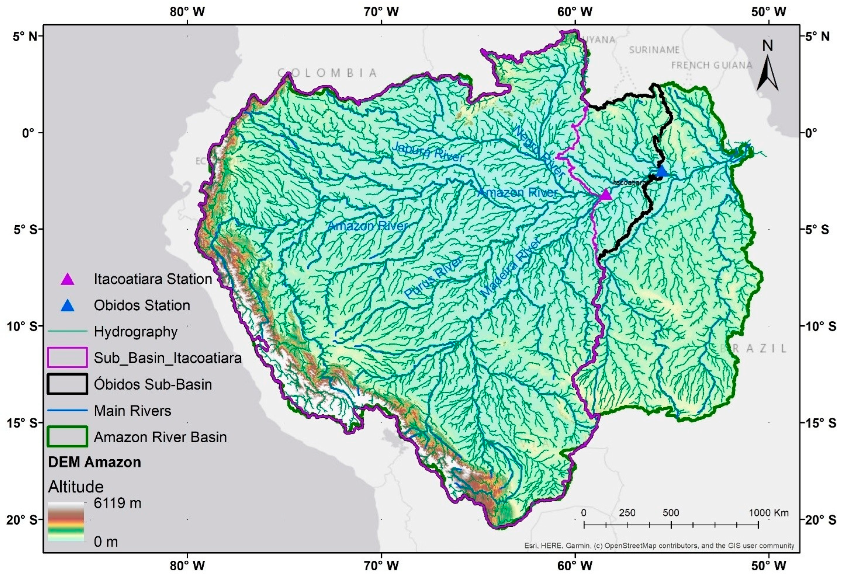
The Óbidos Strait is the last station in the Amazon River where discharge is measured, as downstream tidal effects influence water levels. The tidal effect is observed in Santarém, mostly between the end of July and the beginning of November, when the river is at lower stages. The Óbidos sub-basin encompasses approximately 75% of the total Amazon River Basin, while Itacoatiara captures approximately 70% (Figure 1).

Figure 1. Location of the Óbidos and Itacoatiara gauging stations in the Amazon River Basin. The Óbidos sub-basin represents approximately 75% of the total basin area, and Itacoatiara approximately 70%.

The downstream stations beyond Óbidos are located approximately 10 h by boat. The influence of the backwater effect at Óbidos, caused by tidal dynamics between the low- and high-water seasons, remains an area of ongoing investigation. This phenomenon is not observed at Itacoatiara [13].

2.2. Hydrological Data

The river segment between Óbidos and Manacapuru, upstream of the Negro River confluence, lacked a measurement station until 2008, when the Itacoatiara station was established and records became available. The addition of the Itacoatiara station improved spatial coverage of hydrological monitoring in the area, although the distance between the two stations (~410 km) remains extremely large. The orthometric elevation at Itacoatiara is 19.01 m, compared to 11.3 m at Óbidos. Despite this long separation, the elevation gradient is minimal, with a hydraulic slope of approximately 1.88 × 10⁻⁵ m/m. The hydraulic gradient is dominated by the river stage (i.e., depth of water) and, in the lower part of the river, also by the tidal effect [14]. The Itacoatiara dataset covers the period from 2008 to 2023, comprising 70 stage–discharge measurements, all obtained using ADCP instruments (Teledyne RD Instruments, San Diego, CA, USA). The Óbidos dataset spans from 1968 to 2023, containing 176 measurements collected using both current meter (earlier records) and ADCP techniques. Prior to modeling, the data were subjected to quality control procedures including consistency checks against historical ranges, visual inspection of stage–discharge scatter plots for anomalous points, and verification of measurement metadata.

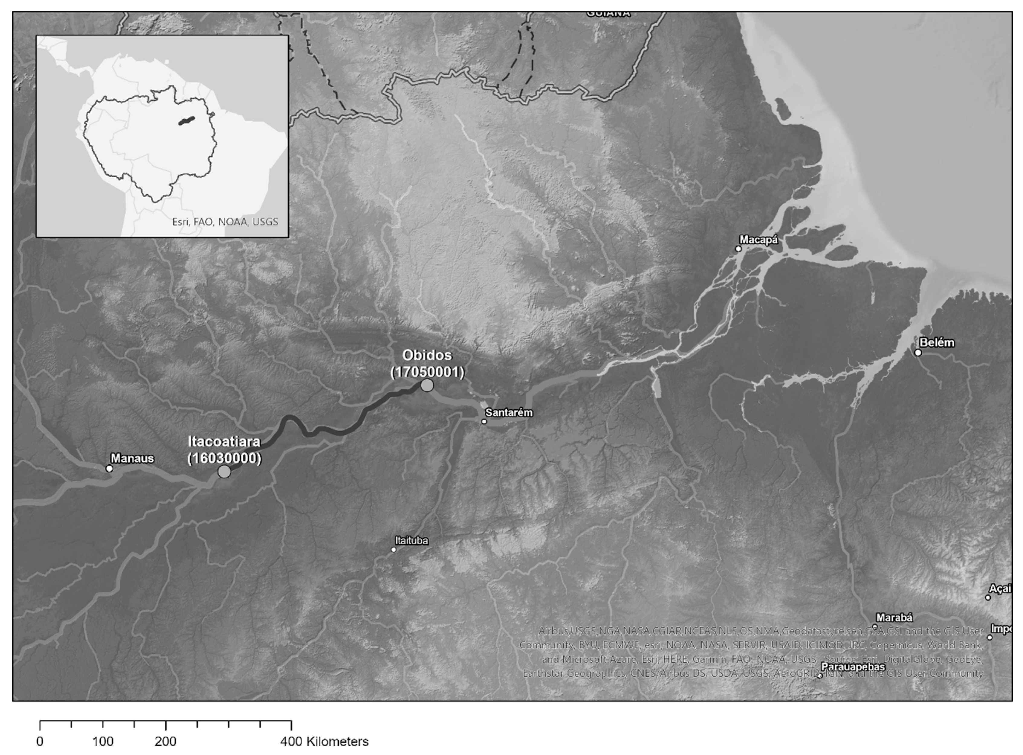
Both stations (Figure 2) use fixed reference levels (arbitrary datums) that have remained consistent throughout the measurement periods, ensuring temporal comparability of all stage readings. All discharge measurements are performed at the same physical location within each station, with fixed initial and final cross-section points. Water level is recorded daily at 07:00 and 17:00 by a local observer, while discharge is measured approximately four times per year: two measurements during the dry season and two during the wet season. The discharge measurements are combined with the daily water level readings to construct the stage–discharge rating curve [4].

Figure 2. Distance between Itacoatiara and Óbidos gauging stations and the spatial distribution of the hydrological network.

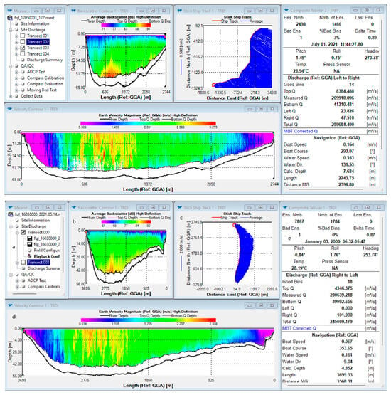
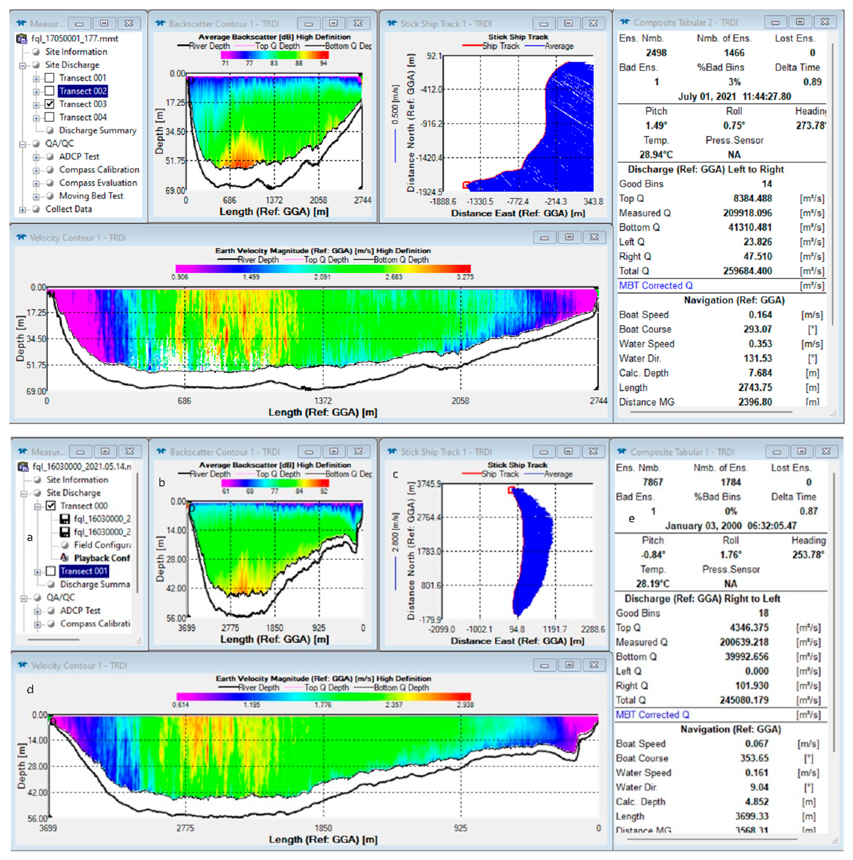
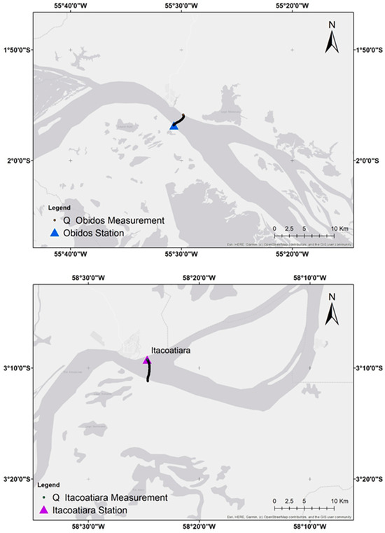
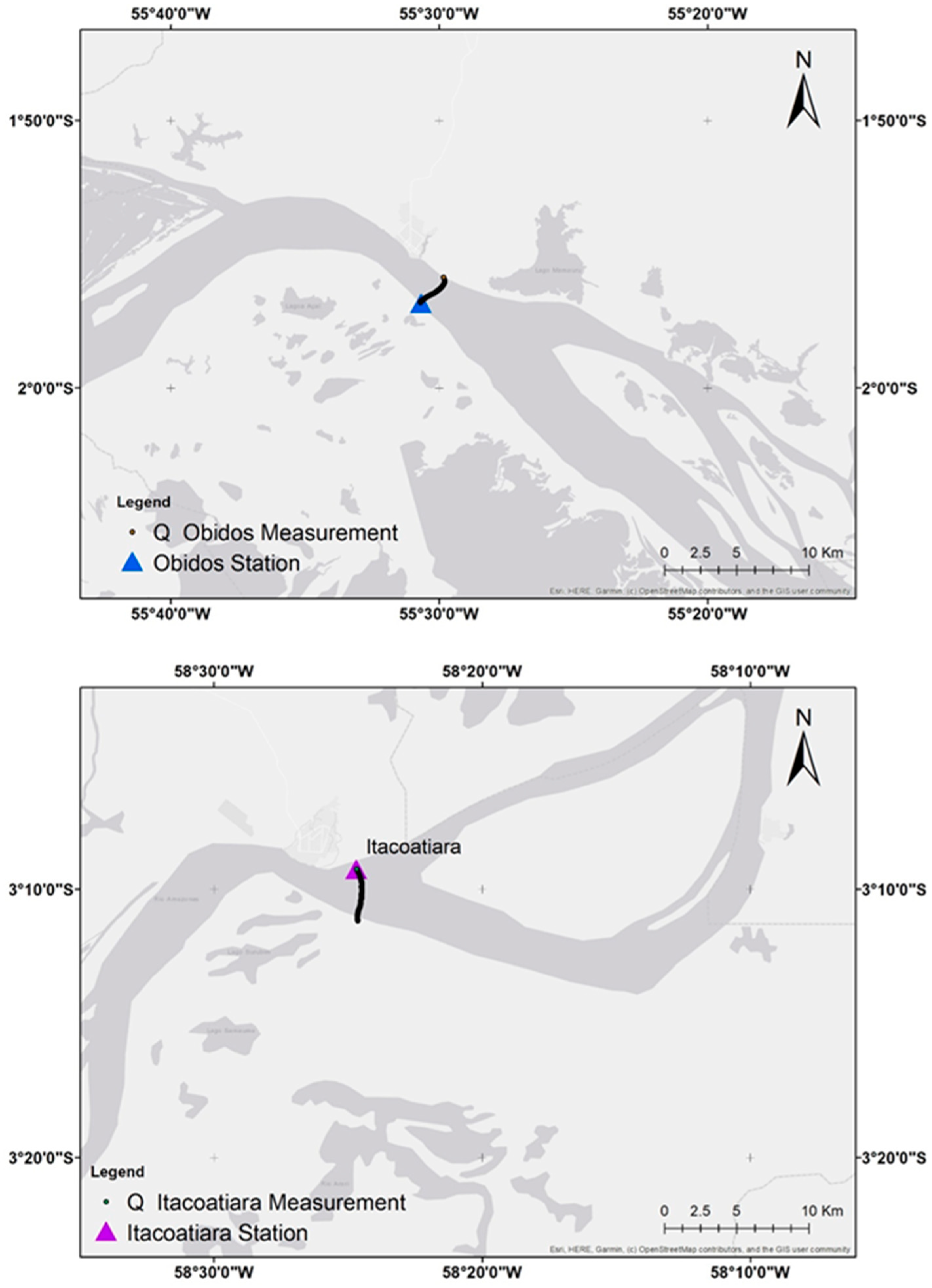
For the two stations, discharge measurements (Figure 3) are performed using two types of Acoustic Doppler Current Profiler (ADCP) instruments, both manufactured by Teledyne RD Instruments (Poway, CA, USA): the Workhorse Rio Grande (600 kHz frequency, 70 m depth range) and the RiverRay (600 kHz frequency, 60 m depth range). These ADCP-based measurements provide velocity profiles and cross-sectional geometry, enabling accurate computation of total discharge. At Óbidos (Figure 4, top), the measured cross-section depth reaches 69 m, the transect length is 2744 m, and velocities exceed 3 m/s. At Itacoatiara (Figure 4, bottom), the deepest point is 56 m, with a transect length of 3699 m. In addition to water level and discharge, the stations also collect sediment discharge and water quality data, which are outside the scope of this study.

Figure 3. The WinRiver II summary screen (RD Instruments) at the end of a complete discharge measurement at Óbidos (top) and Itacoatiara (bottom), showing the key parameters recorded in the field: (a) transect measurement files, (b) beam intensity and depth, (c) boat crossing the measurement point of the established cross-section, (d) main results from the acoustic measurement, and (e) length, area, water velocity, and cells measured including averages.

Figure 4. Local setting of the Óbidos (top) and Itacoatiara (bottom) gauging stations and their respective cross-sectional positions (consecutive dots forming a black line) along the Amazon River.

There is no tangible difference in discharge between the two stations during the dry season despite the 410 km distance. However, during the wet season, the lateral inflow from floodplain dynamics and minor tributaries—including the Uatumã, Urubu, Andirá, Nhamundá, and Trombetas Rivers—produces a noticeable increase in discharge at Óbidos relative to Itacoatiara, with differences reaching approximately 40,000 m³/s during high-flow periods.

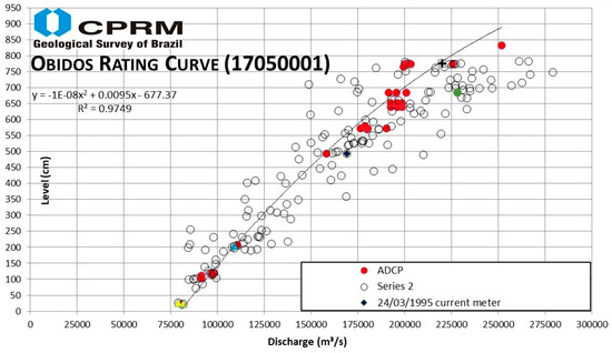
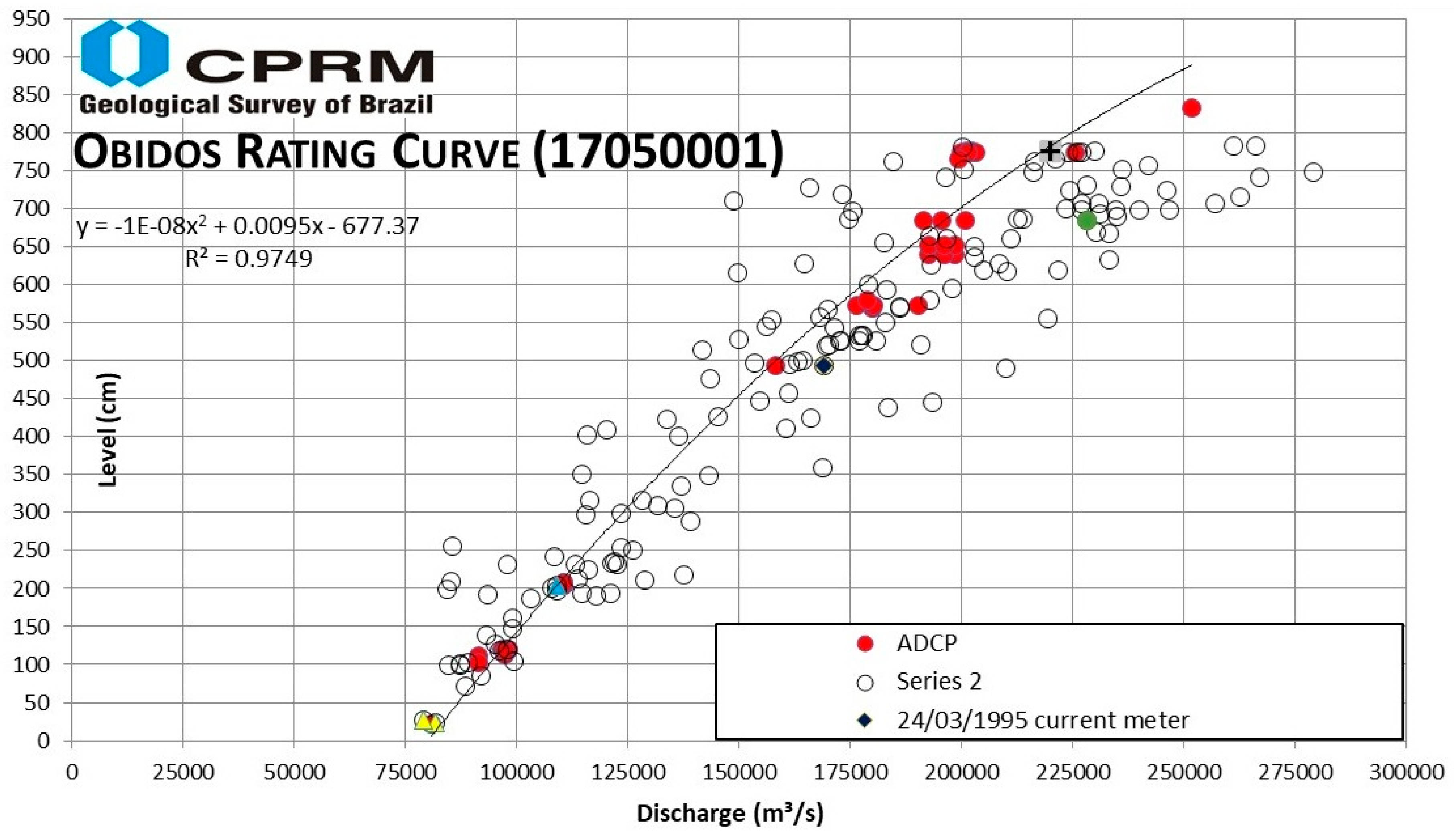
The data (Figure 5) were obtained from the ANA public portal (https://www.snirh.gov.br/hidroweb). CPRM operates the hydrological network, collects the data and performs all field measurements, which are then made available through ANA’s data portal [4].

Figure 5. Rating curve and associated discharge measurements from CPRM for the Óbidos station, as officially published.

2.3. Virtual Stations (Satellite Altimetry)

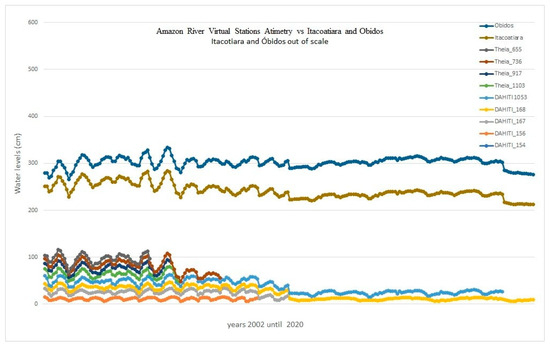
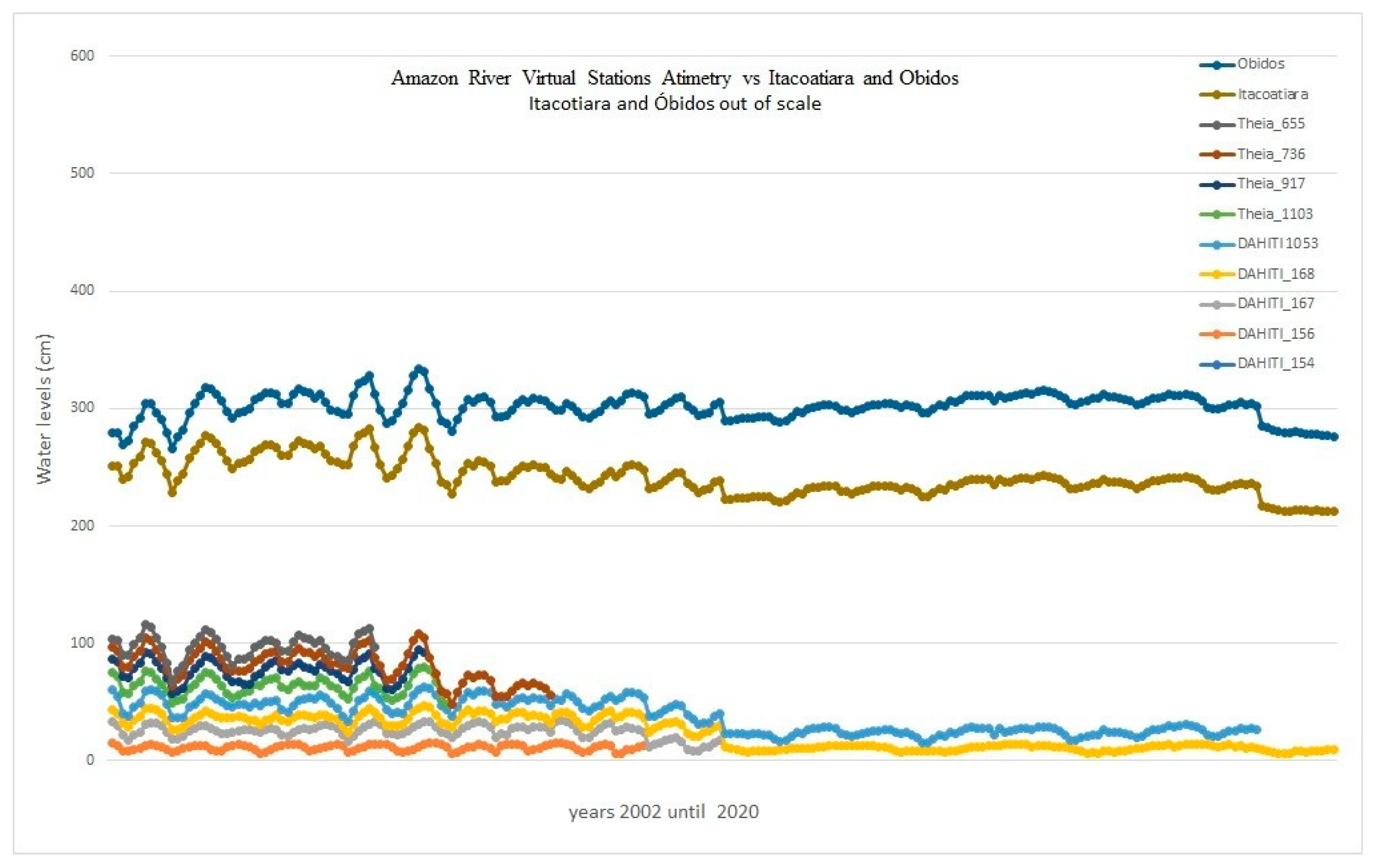
Satellite altimetry data were used to provide independent verification of in situ water level records between gauging stations. In this study, the remote sensing component serves a contextual and validation role rather than an analytical one: altimetry data are not used as a direct input to the rating curve models but instead offer an independent reference for assessing consistency of in situ observations. Virtual stations were obtained from the Database for Hydrological Time Series of Inland Waters (DAHITI) [15] and Hydroweb [16]. These satellite-derived water level measurements provide an independent source of validation data (Figure 6) and help characterize the spatial variability of water levels along the river reach between Itacoatiara and Óbidos. A qualitative comparison between the virtual station records and the in situ gauge data shows good agreement: the satellite-derived water levels at both stations follow the same seasonal patterns and are consistent in magnitude with the gauge observations, reinforcing confidence in the ground-based dataset used for model training and evaluation. While the accuracy of satellite altimetry is generally lower than that of in situ gauges, the data are valuable for assessing water level gradients and verifying the consistency of ground-based observations over the study period. The inclusion of satellite altimetry demonstrates how remote sensing observations can complement conventional hydrological networks in large, data-sparse basins such as the Amazon Basin.

Figure 6. Water levels at virtual stations across the Amazon River Basin, sourced from the Database for Hydrological Time Series of Inland Waters (DAHITI). Stations at Óbidos (blue, top line) and Itacoatiara (brown, second line) record water levels an order of magnitude greater than all other stations in the basin.

2.4. Discharge Summary Statistics

Table 1 presents the summary statistics for discharge and water level at both stations. The Itacoatiara record, which began in 2008, contains 70 paired measurements, while Óbidos has a longer record with 176 measurements. Both stations exhibit strong seasonal patterns, with discharge ranging from approximately 81,000 m³/s to 243,000 m³/s at Itacoatiara and from 60,000 m³/s to 279,000 m³/s at Óbidos. The higher maximum discharge at Óbidos reflects the additional contributions from lateral inflow and tributaries downstream of Itacoatiara. The standard deviation is notably higher at Óbidos (51,484 m³/s) compared to Itacoatiara (45,800 m³/s), reflecting the longer time series and greater hydrological variability captured in the record.

Table 1. Summary statistics of discharge and water level at Itacoatiara and Óbidos.

Statistic	Itacoatiara Q (m3/s)	Itacoatiara h (cm)	Óbidos Q (m3/s)	Óbidos h (cm)
Minimum	81,378	358	59,678	23
25th percentile	140,827	886	123,203	257
Median	182,079	1212	170,740	534
Mean	174,483	1097	167,858	488
75th percentile	209,512	1368	208,851	694
Maximum	242,885	1518	279,000	835
Std. Dev.	45,800	341	51,484	226
N records	70		176

Table 2 presents the official rating curves for both stations, as provided by CPRM. These rating curves, based on the power law equation Q = a(h − h₀)ⁿ, serve as the baselines for comparison with the alternative modeling approaches evaluated in this study.

Table 2. Parameters of the official Itacoatiara and Óbidos rating curves (power law equation) provided by ANA/CPRM.

Parameter	Itacoatiara	Óbidos
a	6452.85	0.32
h0	4.63	22
n	1.204	4
Q mean observed (m3/s)	174,483	167,858

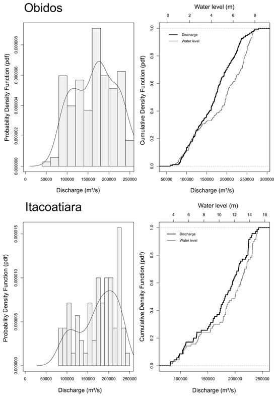
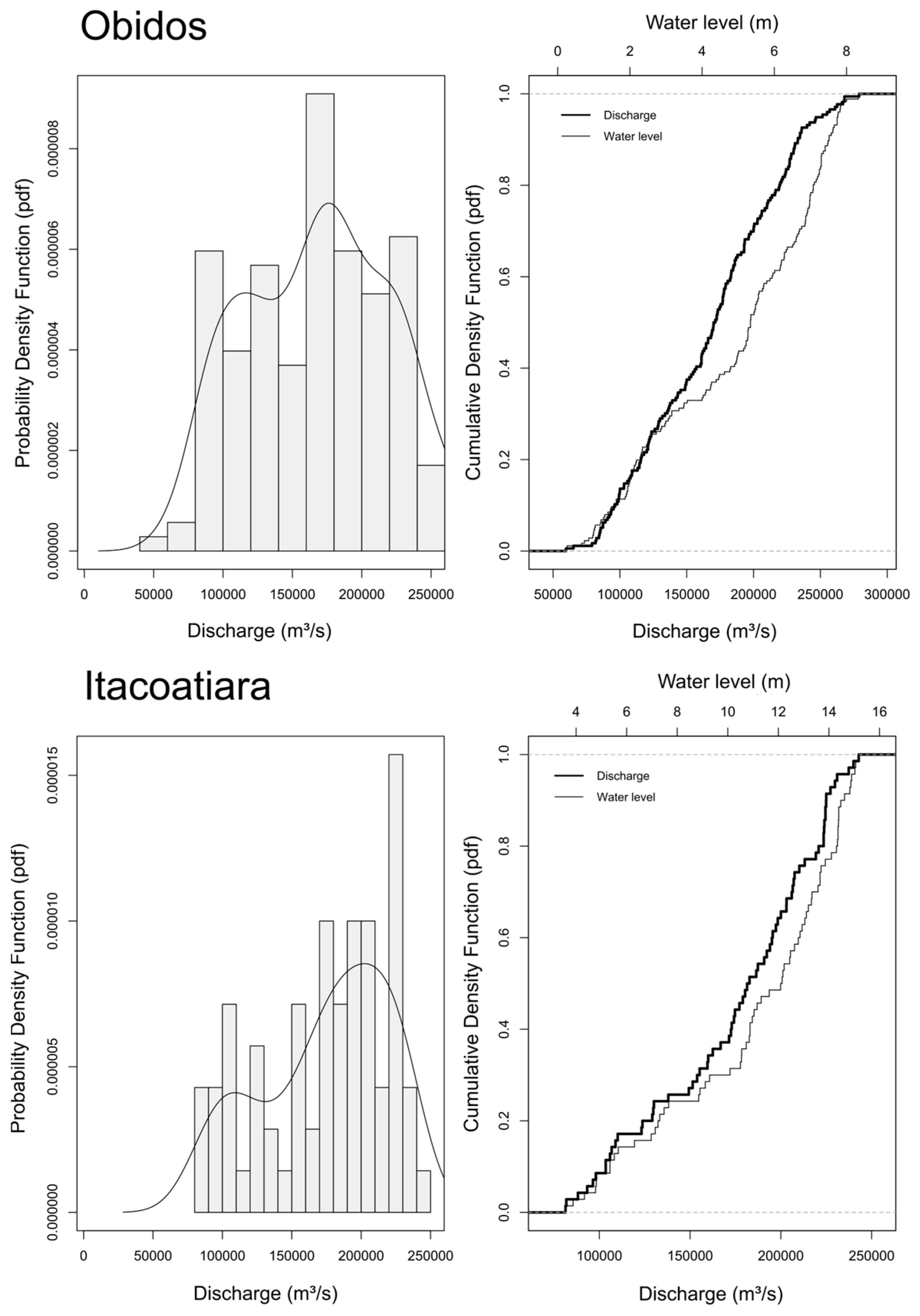
At Óbidos, the CDF (Figure 7) reveals a slight discrepancy in the middle and upper portions of the curve, attributable to scattered measurement values. Some modeling approaches address this by segmenting the rating curve into independent sections. However, this research applies a single rating curve across the full range of observations. At Itacoatiara, the CDFs of water level and discharge are closely related, which is beneficial for fitting an optimal rating curve model.

Figure 7. Probability density function (PDF (left)) and Cumulative Distribution Function (CDF (right)) plots of water level and discharge for Óbidos (top) and Itacoatiara (bottom).

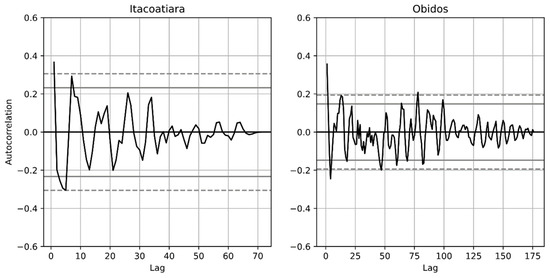
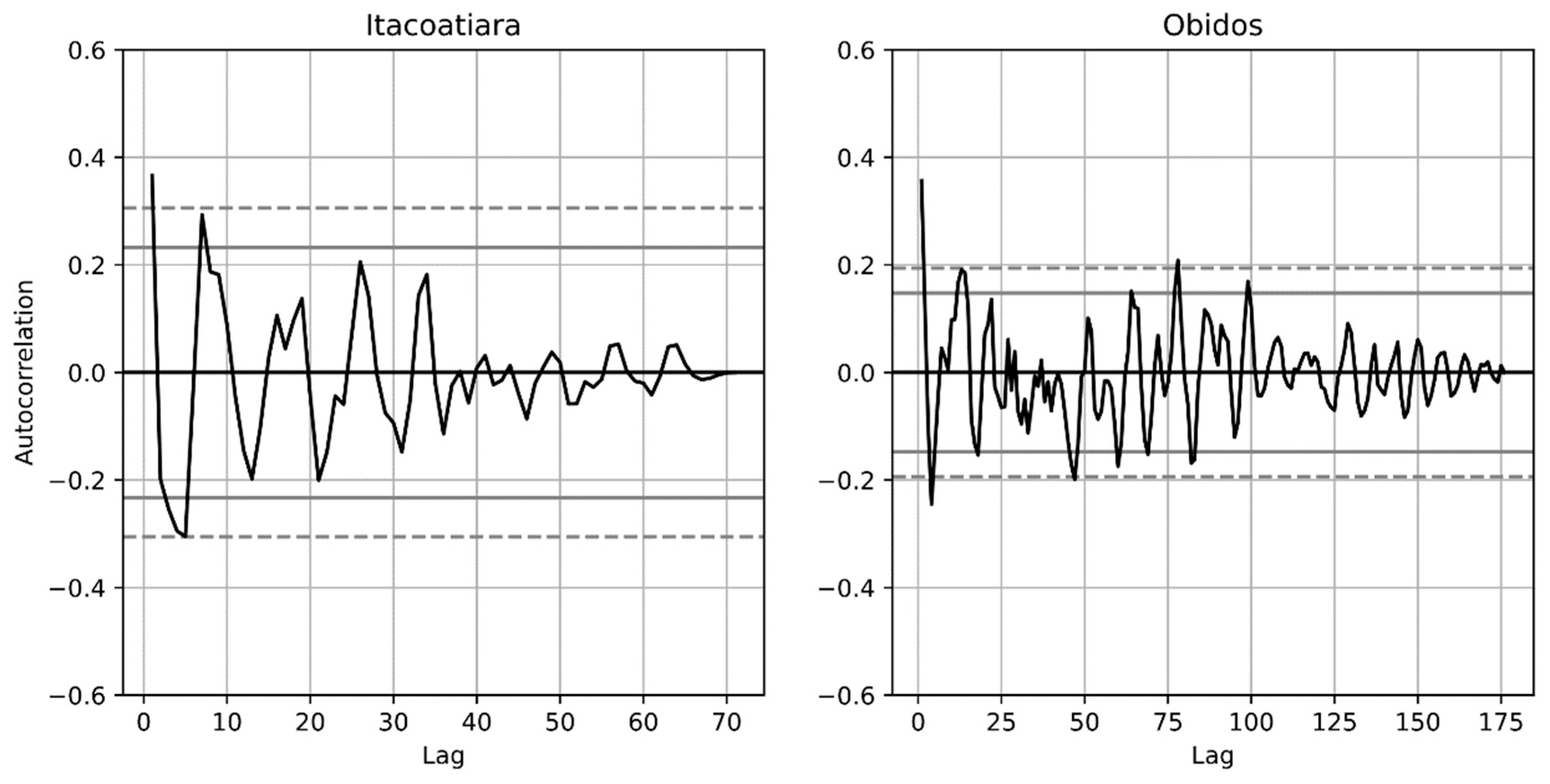
Figure 8 shows the autocorrelation plots for both stations. At Itacoatiara, the autocorrelation decays smoothly toward zero within approximately 70 days, indicating greater stationarity and a well-behaved correlation structure. At Óbidos, the longer time series extends to nearly 175 days and exhibits more variation over time, yet the autocorrelation values remain largely within the confidence bounds. In both stations, the autocorrelation stays within acceptable limits, with only minor exceedances, which is a favorable indicator for model convergence. The consistency of measurements at each station contributes to this strong autocorrelation structure, as temporal variation between successive observations remains smooth.

Figure 8. Autocorrelation of discharge measurements as a function of lag (days) for the Itacoatiara (left) and Óbidos (right) stations.

2.5. Modeling Approaches for Rating Curves

The stage–discharge relationships at the Óbidos and Itacoatiara stations were modeled using two conventional curve-fitting methods: (1) Power Law and (2) Linear Regression, and four machine learning algorithms: (1) Decision Tree, (2) Random Forest, (3) XGBoost, and (4) Multi-Layer Perceptron (MLP). The results obtained from all six modeling approaches were compared against the baseline rating curve equation currently used by ANA and CPRM. This official rating curve is based on a power law equation with coefficients derived from historical discharge measurements. The use of the baseline as a benchmark allows estimation of the improvements offered by the alternative modeling techniques.

2.5.1. Baseline

The baseline rating curves were developed by ANA/CPRM using a power law equation. For Itacoatiara, valid for water levels between 300 cm and 1530 cm, the baseline equation is:

Q = 6452.85(h − 4.63)^1.204

(1)

For Óbidos, valid for water levels between −50 cm and 900 cm:

Q = 0.32(h − 22)⁴

(2)

2.5.2. Power Law

The power law equation is the most commonly applied model for rating curve development in Brazil and is widely adopted by hydrological services across South American countries [4,17]. This nonlinear equation (Equation (3)) uses two parameters, a and n, and incorporates the difference between the observed water level and a reference elevation or datum (h − h₀) to estimate discharge:

Q = a(h − h₀)ⁿ

(3)

2.5.3. Linear Regression

The linear regression model represents the simplest of the traditional rating curve approaches, assuming a direct linear relationship between discharge and water level. This method (Equation (4)) employs two fitting coefficients, m and b:

Q = m(h − h₀) + b

(4)

2.5.4. Decision Tree

The Decision Tree algorithm is a supervised machine learning method that recursively partitions the input space through a series of binary decisions. The algorithm was popularized by Quinlan’s C4.5 system [18], building on earlier work such as Breiman et al.’s CART (Classification and Regression Trees) method [19]. In a decision tree, the input data are split at specific thresholds of the predictor variable (in this case, water level), guiding the model along different branches to estimate the target variable (discharge).

At each internal (non-leaf) node, the algorithm selects the test that most effectively discriminates between subsets of the data. C4.5 uses information gain criteria based on information theory to evaluate the quality of each potential split, choosing the test that extracts the maximum information from the data at that node [18]. For regression tasks such as rating curve estimation, the algorithm minimizes the variance of the target variable within each partition. Each leaf node contains a predicted value, typically the mean discharge of the training instances that fall within that partition.

A key consideration with decision trees is the risk of overfitting, the scenario in which a tree that perfectly classifies every training example may not generalize well to unseen data. To mitigate this, most decision tree algorithms employ pruning methods, which grow a large tree and then remove branches that do not improve generalization performance [18]. The Decision Tree exhibited overfitting that could not be mitigated through pruning, depth limitation, or alternative regularization strategies given the limited sample size. Its results are reported for completeness but were excluded from the final model comparison. In this study, the decision tree was configured with a maximum depth of 5 levels for Itacoatiara and 4 levels for Óbidos. The tree-based structure captures nonlinear relationships between stage and discharge by recursively partitioning the data at these decision points, making it well-suited for modeling the nonlinear stage–discharge relationship in large rivers.

2.5.5. Random Forest

Random Forest is an ensemble machine learning algorithm introduced by Breiman [20] that aggregates the predictions of multiple decision trees to improve accuracy and reduce overfitting. The method constructs a collection of tree-structured predictors, where each tree is grown using a randomly sampled subset of the training data (bootstrap sampling) and a random subset of features at each split node. Formally, a Random Forest is defined as a classifier consisting of a collection of tree-structured classifiers composed of independent identically distributed random vectors [20].

A fundamental property of Random Forests, demonstrated by Breiman [20] through the Strong Law of Large Numbers, is that the generalization error converges to a limit as the number of trees increases. This means that Random Forests do not overfit as more trees are added—instead, they produce a limiting value of the generalization error. The accuracy of a Random Forest depends on two key factors: the strength (accuracy) of the individual trees and the correlation between them [20]. Reducing the correlation between trees (through randomization) while maintaining individual tree accuracy leads to better ensemble performance.

For rating curve modeling, each tree in the Random Forest independently models the stage–discharge relationship, and the final discharge prediction is obtained by averaging the outputs of all individual trees. This averaging process smooths out the noise and variance inherent in individual decision trees, generally producing more robust predictions than a single tree. The Random Forest model was implemented using standard hyperparameter tuning, with the number of trees and maximum depth optimized through cross-validation. Specifically, the Random Forest was configured with a minimum sample leaf of 4 and a maximum depth of 6.

2.5.6. XGBoost

Extreme Gradient Boosting (XGBoost) is a scalable end-to-end tree boosting system introduced by Chen and Guestrin [21]. Unlike Random Forest, which builds trees independently and averages their predictions, XGBoost constructs an ensemble of sequential decision trees in which each subsequent tree is trained to correct the residual errors of the preceding ensemble. The method has achieved state-of-the-art results across numerous machine learning benchmarks and data science competitions [21].

For a given dataset with n examples and m features, XGBoost uses K additive functions to predict the output, where each function corresponds to an independent regression tree [21]. The model minimizes a regularized objective function that includes both a loss term and a penalty for model complexity. The loss function measures the difference between the prediction and the target. This regularization term, which includes penalties on the number of leaves and the magnitude of leaf weights, helps prevent overfitting and is a key distinguishing feature of XGBoost compared to traditional gradient boosting implementations [21]. The algorithm employs a second-order Taylor expansion of the loss function to efficiently determine optimal tree structures and leaf weights, and uses a greedy algorithm that iteratively adds branches to the tree based on the information gain at each split point.

For rating curve modeling, XGBoost progressively refines the stage–discharge estimate by building each tree to reduce the prediction errors from previous trees. This boosting approach can capture complex nonlinear patterns in the data, while the regularization framework helps maintain generalization capability. The XGBoost model was configured with the following hyperparameters: learning rate of 0.1, 100 estimators, and minimum sample leaf of 4.

2.5.7. Multi-Layer Perceptron (MLP) Regressor

The Multi-Layer Perceptron (MLP) regressor is a type of feedforward artificial neural network consisting of multiple layers of interconnected neurons: an input layer, one or more hidden layers, and an output layer [6,7]. Each neuron in the hidden layers applies a nonlinear activation function to a weighted sum of its inputs, allowing the network to learn complex nonlinear mappings between water level and discharge data.

The MLP is trained using backpropagation and gradient descent optimization, which iteratively adjusts the network weights to minimize a loss function (typically mean squared error for regression tasks). The architecture used in this study consisted of an input layer receiving the water level (stage) value, two hidden layers with rectified linear unit (ReLU) activation functions, and an output layer producing the discharge estimate. The number of neurons in the hidden layers and the learning rate were tuned through cross-validation. Neural networks have been previously applied to stage–discharge modeling with promising results [6,7], though their performance can be sensitive to the choice of hyperparameters and the size of the training dataset. Specifically, the MLP regressor was configured with 75,000 maximum number of iterations and a constant learning rate.

2.6. Statistical Metrics

The performance of the modeling approaches was assessed using four statistical metrics: Root Mean Square Error (RMSE), coefficient of determination (r²), Mean Bias Error (MBE), Nash–Sutcliffe Efficiency (NSE) and Kling–Gupta Efficiency (KGE). For the machine learning methods (Decision Tree, Random Forest, XGBoost, and MLP), a k-fold cross-validation with 3 splits was implemented to evaluate predictive accuracy:

2.6.1. Root Mean Square Error (RMSE)

RMSE quantifies the standard deviation of prediction errors, providing a measure of the magnitude of the residuals. It is expressed in the same units as the predicted variable, making it directly interpretable:

$$RMSE=\sqrt{{\displaystyle \frac{1}{n}}{\sum }_{i=1}^n{\left(Q_{p,i}-Q_{o,i}\right)}^2}$$

(5)

where $n$ is the number of observations, $Q_{p,i}$ is the predicted (i.e., modeled) value, and $Q_{o,i}$ is the observed value, both at time step $i$.

2.6.2. Coefficient of Determination (r²)

The coefficient of determination r² indicates the proportion of variance in the observed discharge explained by the model.

$$r^2={\displaystyle \frac{\sum _{\mathrm{i}=1}^{\mathrm{n}}{\left({\mathrm{Q}}_{\mathrm{o},\mathrm{i}}-{\mathrm{\mu }}_{\mathrm{p}}\right)}^2}{\sum _{\mathrm{i}=1}^{\mathrm{n}}{\left({\mathrm{Q}}_{\mathrm{p},\mathrm{i}}-{\mathrm{\mu }}_{\mathrm{o}}\right)}^2}}$$

(6)

where ${\mu }_o$ and ${\mu }_p$ are the mean values of the observed and predicted series respectively.

2.6.3. Mean Bias Error (MBE)

MBE measures the systematic tendency to overestimate (positive MBE) or underestimate (negative MBE) discharge.

$$\begin{array}{c}MBE={\displaystyle \frac{1}{n}}\sum _{i=1}^n(Q_{p,i}-Q_{o,i})\end{array}$$

(7)

2.6.4. Nash–Sutcliffe Efficiency (NSE)

NSE evaluates how well the model predictions match the observed data relative to a simple mean model, where NSE = 1 indicates perfect agreement and NSE < 0 indicates the model performs worse than the observed mean [22].

$$NS=1-{\displaystyle \frac{{\sum }_{i=1}^n(Q_{o,i}-{\mathrm{Q}}_{p,i}{)}^2}{{\sum }_{i=1}^n(Q_{o,i}-{\mathrm{\mu }}_{\mathrm{o}}{)}^2}}$$

(8)

The baseline metrics using the CPRM official rating curves are for Óbidos: RMSE = 25,267 m³/s, r² = 0.894, MBE = −6091, and NSE = 0.784 and for Itacoatiara: RMSE = 12,188 m³/s, r² = 0.967, MBE = −3456, and NSE = 0.927.

2.6.5. Kling–Gupta Efficiency (KGE)

KGE provides a measure of model performance by simultaneously evaluating correlation, bias, and variability between predicted and observed values, where KGE = 1 indicates perfect agreement and increasingly negative values indicate poor performance [23].

$$KGE=1-\sqrt{{\left(r^2-1\right)}^2+{\left({\displaystyle \frac{{\sigma }_p}{{\sigma }_o}}-1\right)}^2+{\left({\displaystyle \frac{{\mu }_p}{{\mu }_o}}-1\right)}^2}$$

(9)

where $r^2$ is the correlation coefficient, and ${\sigma }_p$ and ${\sigma }_o$ are the standard deviations of the observed and predicted series respectively.

2.6.6. K-Fold Cross-Validation

Cross-validation was performed using a 3-fold partitioning scheme with model hyperparameters fixed a priori for each algorithm; no parameter tuning occurred within the validation loop to avoid data leakage. The choice of 3 folds was constrained by the limited sample size, particularly at Itacoatiara (n = 70), where higher fold counts would yield training subsets too small for stable model fitting; nevertheless, the consistency of performance metrics across folds supports the reported results.

3. Results

This section presents the results of the rating curve modeling for both stations. The performance of each method is evaluated through comparison of the statistical metrics against the official ANA/CPRM baseline, and the results are illustrated through stage–discharge plots.

3.1. Itacoatiara Station

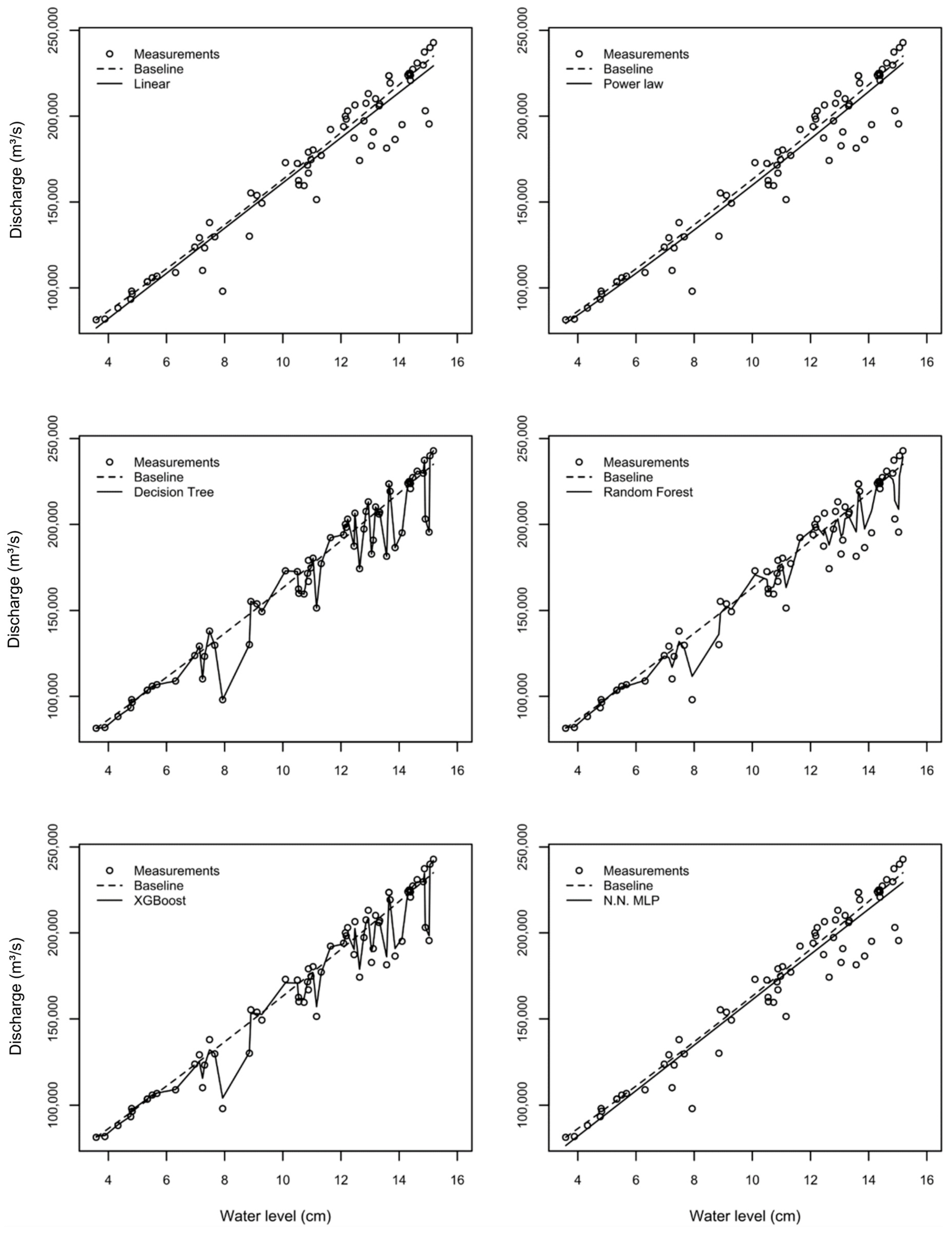
The statistical metrics for the rating curve models at Itacoatiara are presented in Table 3. The machine learning methods—Decision Tree, Random Forest, and XGBoost—consistently outperformed, albeit marginally, the traditional methods and the official baseline. Among the models, XGBoost was selected as the best performer with an RMSE of 7463 m³/s, r² of 0.987, MBE of 0, and NSE of 0.973, indicating an excellent fit with minimal bias.

Table 3. Performance metrics for rating curve models at Itacoatiara. Cross-validation variability for machine learning methods is reported as the mean value and standard deviation (in parentheses) across folds.

Model	RMSE [m3/s]	r2	MBE [m3/s]	NSE	KGE
Baseline	12,188	0.967	−3456	0.927	0.965
Linear	11,748	0.967	0	0.93	0.957
Power Law	11,669	0.967	16	0.932	0.958
Decision Tree	9850 (±4782)	0.976 (±0.12)	0	0.953 (±0.12)	0.966 (±0.06)
Random Forest	9990 (±3038)	0.975 (±0.09)	169	0.952 (±0.09)	0.959 (±0.01)
XGBoost	7463 (±3393)	0.987 (±0.11)	0	0.973 (±0.11)	0.972 (±0.03)
MLP	11,006 (±5131)	0.970 (±0.11)	6	0.941 (±0.11)	0.958 (±0.03)

Decision Tree had an RMSE (9850 m³/s), r² (0.976), and NSE (0.953). However, the fit plot strongly suggests overfitting, whereby the reduced sample size causes the model to memorize the training data rather than learn generalizable patterns, so it was discarded. This is an important limitation that should be considered when interpreting these results [18,20].

Random Forest also showed improvement over traditional methods (RMSE = 9990 m³/s, NSE = 0.952), though with a small bias (MBE = 169 m³/s). The traditional methods (Linear Regression, Power Law, and MLP) all performed similarly to the baseline, with RMSE values around 11,700 m³/s and NSE values near 0.960. Notably, the MLP neural network did not outperform the simple linear or power law models at this station with a large standard deviation in the k-fold test (5131 m³/s), suggesting that the limited training dataset (70 records) may be insufficient for the neural network to learn meaningful complex patterns beyond what simpler models capture. The MBE values of zero for Linear Regression, Decision Tree, and XGBoost indicate minimal systematic bias, whereas the baseline exhibited an MBE of −3456 m³/s, suggesting a systematic underestimation of discharge.

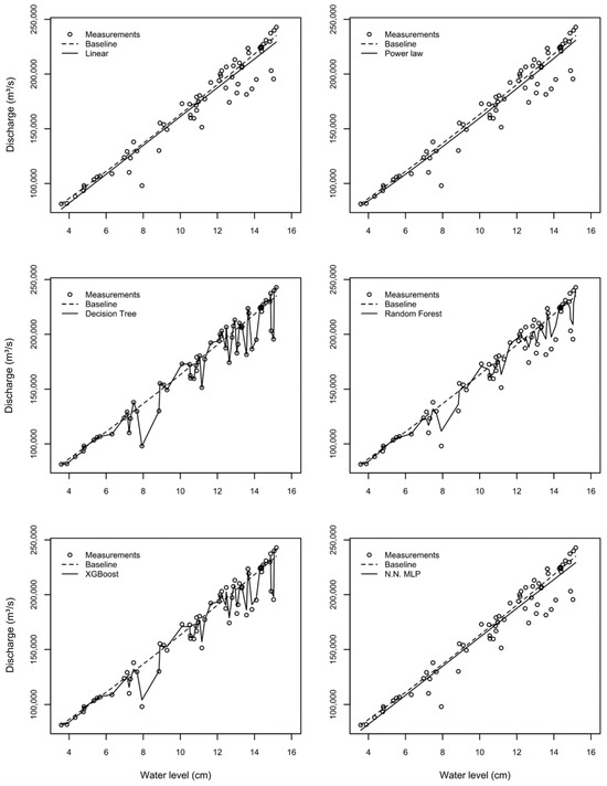
Figure 9 shows the stage–discharge relationships for all models at Itacoatiara compared to the baseline. The plots confirm that the Decision Tree, XGBoost, and Random Forest models cluster closely around the observed data, while the traditional methods (Linear, Power Law, and MLP) follow similar trajectories that diverge from observed values, particularly at the extremes of the discharge range. The Decision Tree for Itacoatiara consisted of five branching levels, partitioning the stage space into distinct regions with optimized discharge estimates.

Figure 9. Rating curve fits for the Itacoatiara station using six modeling approaches: Linear (RMSE: 11,748), Power Law (RMSE: 11,669), Decision Tree (RMSE: 9850), Random Forest (RMSE: 9990), XGBoost (RMSE: 7463), and Neural Network MLP (RMSE: 11,006). The dashed line represents the baseline model (RMSE: 12,188).

3.2. Óbidos Station

The performance metrics for Óbidos (Table 4) follow a similar pattern to Itacoatiara, but with notably larger errors across all methods. This is expected given the longer time series (176 measurements spanning several decades), greater hydrological variability, and the inclusion of measurements from both ADCP and earlier current meter techniques. The larger spread in the observed stage–discharge data at Óbidos directly impacts the error metrics and overall model fit.

Table 4. Performance metrics for rating curve models at Óbidos. Cross-validation variability for machine learning methods is reported as the mean value and standard deviation (in parentheses) across folds.

Model	RMSE [m3/s]	r2	MBE [m3/s]	NSE	KGE
Baseline	25,267	0.894	−6091	0.784	0.873
Linear	22,915	0.895	0	0.751	0.851
Power Law	22,928	0.895	−68	0.748	0.848
Decision Tree	19,716 (±3239)	0.923 (±0.11)	0	0.853 (±0.11)	0.892 (±0.04)
Random Forest	20,302 (±3495)	0.919 (±0.11)	319	0.844 (±0.11)	0.876 (±0.06)
XGBoost	18,378 (±3139)	0.934 (±0.10)	0	0.872 (±0.10)	0.888 (±0.04)
MLP	22,915 (±3467)	0.895 (±0.09)	2	0.801 (±0.09)	0.851 (±0.07)

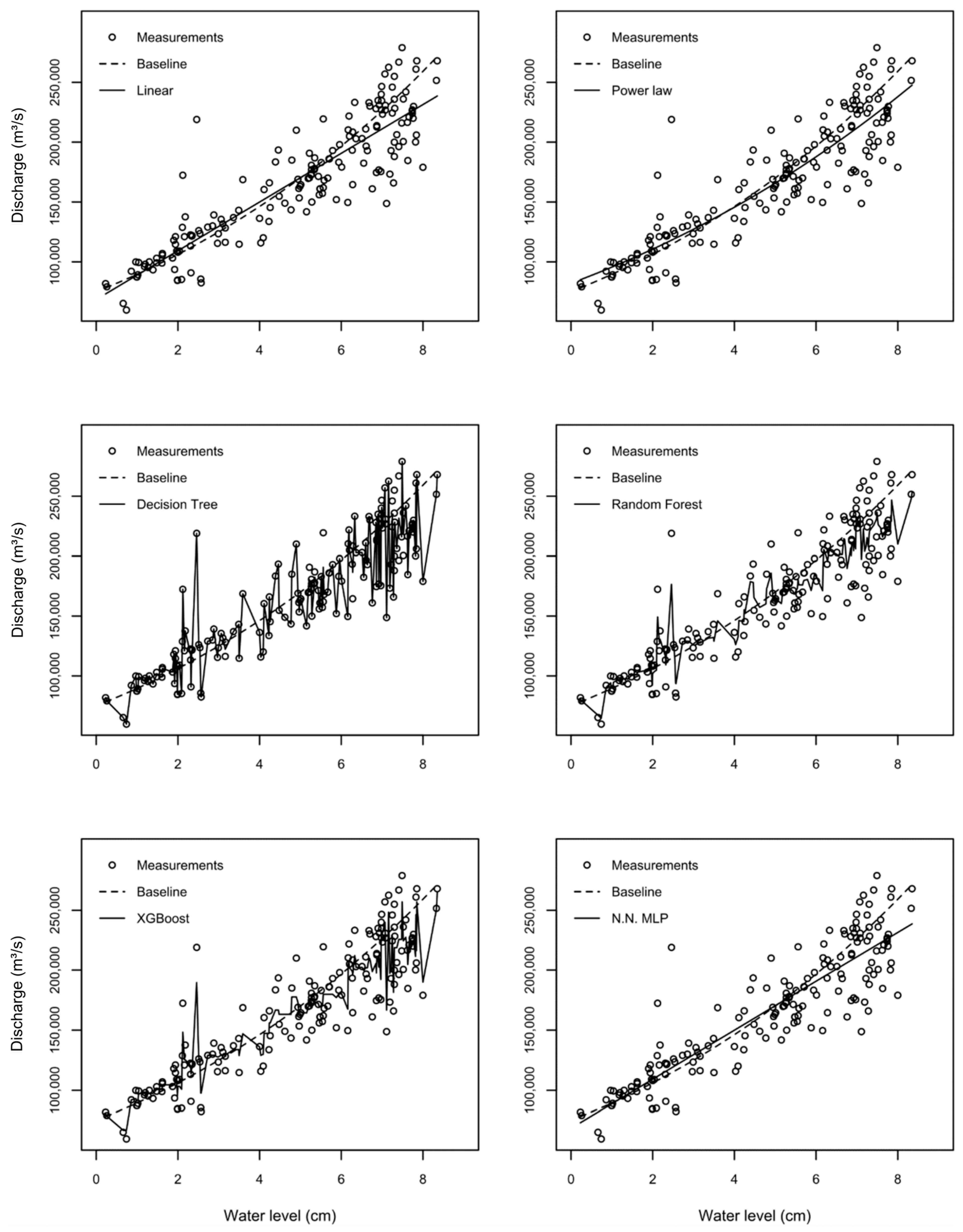
XGBoost was selected best model (RMSE = 18,378 m³/s, r² = 0.934, NSE = 0.872), followed by Random Forest (RMSE = 20,302 m³/s, r² = 0.919, NSE = 0.844). All machine learning models performed slightly better than the traditional methods and the baseline. The Decision Tree again showed signs of overfitting in the rating curve plot with RMSE (19,716 m³/s), r² (0.923), NSE (0.853), and zero bias. As with Itacoatiara, the Decision Tree for Óbidos likely exhibits overfitting behavior given the fit, so it was discarded.

The traditional methods performed weaker at Óbidos compared to Itacoatiara. The baseline showed an RMSE of 25,267 m³/s and NSE of 0.784, while the linear and power law models had RMSE values around 22,900 m³/s and NSE values near 0.75. The significant negative MBE of the baseline (−6091 m³/s) suggests a systematic underestimation of discharge by the official rating curve, which may be related to changes in the river cross-section morphology over the extended measurement period. The MLP neural network performed as the linear regression model (RMSE = 22,915 m³/s, NSE = 0.801), again indicating limited benefit from the neural network architecture with the available dataset.

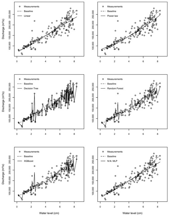
The stage–discharge relationship at Óbidos (Figure 10) is more scattered than at Itacoatiara, reflecting the greater variability of this station due to the larger sample size. Among all methods tested, XGBoost provides the best performance, with an RMSE of 18,378 m³/s, representing an improvement over the baseline (RMSE: 25,267 m³/s) and outperforming both Random Forest (RMSE: 20,302 m³/s) and the traditional approaches: Linear (RMSE: 22,915 m³/s) and Power Law (RMSE: 22,928 m³/s). This positions XGBoost as the most reliable and generalizable model for the Óbidos rating curve.

Figure 10. Rating curve fits for the Óbidos station using six modeling approaches: Linear (RMSE: 22,915), Power Law (RMSE: 22,928), Decision Tree (RMSE: 19,716), Random Forest (RMSE: 20,302), XGBoost (RMSE: 18,378), and Neural Network MLP (RMSE: 22,915). The dashed line represents the baseline model (RMSE: 25,267).

4. Discussion

Machine learning was used to model the rating curves for the Itacoatiara and Óbidos gauging stations on the Amazon River. The machine learning models—Decision Tree, XGBoost, Random Forest, and MLP—showed smaller errors and less bias than the traditional methods (Linear Regression and Power Law) at both stations. The traditional methods, especially the baseline power law equation, already exhibited strong performance, making the machine learning methods’ improvements marginal. In addition, all models were compared against the CPRM baseline, and all approaches performed better than the official rating curve. This finding reaffirms the common understanding that rating curve parameters should be re-fitted and refined periodically to maintain accuracy, especially in dynamic river systems like the Amazon [17,24].

The length of the time series influences the machine learning results. At Itacoatiara, where the record is shorter (70 measurements since 2008) and more homogeneous (all ADCP-based), the models achieved substantially lower errors compared to Óbidos. The longer and more heterogeneous Óbidos record (176 measurements combining current meter and ADCP techniques spanning several decades) introduces greater scatter in the stage–discharge relationship, leading to larger RMSE values across all methods. The standard deviation of discharge at Óbidos (51,484 m³/s) is approximately 12% higher than at Itacoatiara (45,800 m³/s), which directly propagates into the error metrics. The limited sample size at Itacoatiara (70 records) is particularly constraining for data-intensive methods such as the MLP neural network, which typically requires substantially larger training sets to learn meaningful nonlinear patterns beyond what simpler parametric models capture. This explains why the MLP did not outperform the Power Law at either station. Furthermore, the heterogeneity of measurement techniques at Óbidos—combining older current meter data with modern ADCP measurements—introduces additional noise into the stage–discharge relationship that affects all models but is especially challenging for ML methods sensitive to data consistency.

On the other hand, the statistical metrics of traditional methods such as the Power Law with optimized parameters were not drastically far from the machine learning results in terms of normalized performance. This suggests that the simplicity of traditional methods still carries advantages for operational use: they can be employed by field technicians without additional training or specialized software. A power law equation can be quickly calculated on site to verify results, whereas machine learning algorithms function somewhat as “black boxes,” requiring computational infrastructure and specialized expertise to implement and interpret [20,21].

The Decision Tree algorithm, while showing good performance at both stations, exhibits signs of overfitting—an inherent risk with tree-based models when applied to limited datasets [18]. The rating curve plot suggests that the tree has essentially memorized the training instances. The practical implication is that these models may produce large errors for water levels outside the range of the training data. As Breiman [20] showed, the generalization error of a Random Forest depends on the correlation between individual trees and their individual accuracy; ensembles like Random Forest and XGBoost partially mitigate this overfitting issue through averaging and regularization, respectively.

XGBoost, with its regularized objective function that penalizes model complexity [21], represents a more balanced approach between prediction accuracy and generalization capability. At both stations, XGBoost achieved excellent metrics (NSE = 0.973 at Itacoatiara, NSE = 0.872 at Óbidos) while avoiding the extreme overfitting behavior of the standalone Decision Tree. For practical applications where the rating curve must extrapolate to ungauged water levels—such as extreme flood or drought events—XGBoost may be the preferred machine learning approach.

No evidence of backwater effects was detected at Itacoatiara, and their influence at Óbidos remains uncertain, but it could be disregarded for rating curve modeling. Nevertheless, future studies should further investigate the potential influence of backwater conditions at downstream locations of Óbidos.

From an operational perspective, the question of whether the added complexity of machine learning justifies the marginal improvement over traditional methods deserves careful consideration. For Óbidos, the Power Law achieves NSE = 0.748 while XGBoost achieves NSE = 0.872, a marginal improvement. However, at Itacoatiara, the Power Law already achieves NSE = 0.967, and XGBoost improves this slightly to NSE = 0.987. For many operational applications, recalculating the Power Law coefficients every few years using the latest discharge measurements may be a pragmatic and sufficient approach, particularly at stations where the traditional methods already perform well. Machine learning methods may be most valuable at stations with greater hydrological complexity, such as Óbidos, where traditional methods show more pronounced limitations.

5. Conclusions

This study evaluated traditional curve-fitting methods and machine learning algorithms for modeling rating curves at the Itacoatiara and Óbidos gauging stations on the Amazon River. The principal findings are as follows:

Machine learning models (Decision Tree, XGBoost, Random Forest) consistently showed smaller errors and less bias than traditional methods (Linear Regression, Power Law, MLP) at both stations. All models outperformed the CPRM baseline rating curves, indicating that periodic re-fitting of rating curve parameters can improve discharge estimation accuracy. Among the machine learning approaches, XGBoost provided the best balance between predictive accuracy and generalization capability, achieving the lowest RMSE values of 7463 m³/s at Itacoatiara and 18,378 m³/s at Óbidos. The Decision Tree, despite achieving low absolute errors, exhibited signs of overfitting that limit its reliability for extrapolation to conditions outside the training range.

The length and homogeneity of the time series significantly influenced model performance, with the shorter but more consistent Itacoatiara record yielding lower errors across all methods compared to the longer but more variable Óbidos record. Traditional methods, particularly the optimized Power Law, remain practical and transparent alternatives for routine operational use, especially at stations where they already achieve adequate performance. The simplicity of a power law equation—which can be applied directly by field technicians without specialized software—represents an important advantage for operational hydrology in remote regions of the Amazon Basin.

Future research should explore the use of additional input variables (e.g., satellite altimetry, upstream discharge, precipitation) in the machine learning models, the application of cross-validation and out-of-sample testing to rigorously assess generalization performance, and the extension of these methods to other gauging stations across the Amazon network. Additionally, investigating the performance of these models for extreme events (floods and droughts) would provide valuable insight into their reliability for emergency management applications.

References

- Marengo, J.A.; Souza, C.M.; Thonicke, K.; Burton, C.; Halladay, K.; Betts, R.A.; Alves, L.M.; Soares, W.R. Changes in Climate and Land Use Over the Amazon Region: Current and Future Variability and Trends. Front. Earth Sci. 2018, 6, 228. [Google Scholar] [CrossRef] [Scilit]
- Braga, B.P.F.; Tundisi, J.G.; Tundisi, T.M.; Ciminelli, V.S.T. Águas Doces No Brasil: Capital Ecológico, Uso e Conservação, 4th ed.; Escrituras: São Paulo, Brazil, 2015. [Google Scholar]
- ANA—Agência Nacional de Águas e Saneamento Básico. Sistema de Alerta de Eventos Críticos (SACE). Available online: https://www.cprm.gov.br/sace/ (accessed on 15 January 2025).
- ANA—Agência Nacional de Águas e Saneamento Básico. HidroWeb: Portal de Dados Hidrológicos. Available online: https://www.snirh.gov.br/hidroweb/ (accessed on 15 January 2025).
- Molinier, M.; Guyot, J.L.; Oliveira, E.; Guimarães, V. Les Régimes Hydrologiques de l’Amazone et de ses Affluents. In L’Hydrologie Tropicale: Géoscience et Outil Pour le Développement; IAHS Publication: Wallingford, UK, 1996; pp. 209–222. [Google Scholar]
- Bhattacharya, B.; Solomatine, D.P. Application of Artificial Neural Network in Stage–Discharge Relationship. In Proceedings of the 4th International Conference on Hydroinformatics, Iowa City, IA, USA, 22–26 July 2000; pp. 1–7. [Google Scholar]
- Bhattacharya, B.; Solomatine, D.P. Neural Networks and M5 Model Trees in Modelling Water Level–Discharge Relationship. Neurocomputing 2005, 63, 381–396. [Google Scholar] [CrossRef] [Scilit]
- Schwatke, C.; Dettmering, D.; Bosch, W.; Seitz, F. DAHITI—An Innovative Approach for Estimating Water Level Time Series over Inland Waters Using Multi-Mission Satellite Altimetry. Hydrol. Earth Syst. Sci. 2015, 19, 4345–4364. [Google Scholar] [CrossRef] [Scilit]
- Sudheer, K.P.; Jain, S.K. Radial Basis Function Neural Network for Modeling Rating Curves. J. Hydrol. Eng. 2003, 8, 161–164. [Google Scholar] [CrossRef] [Scilit]
- Wolfs, V.; Willems, P. Development of Discharge-Stage Curves Affected by Hysteresis Using Time Varying Models, Model Trees and Neural Networks. Environ. Model. Softw. 2014, 55, 107–119. [Google Scholar] [CrossRef] [Scilit]
- Rozos, E.; Leandro, J.; Koutsoyiannis, D. Development of Rating Curves: Machine Learning vs. Statistical Methods. Hydrology 2022, 9, 166. [Google Scholar] [CrossRef] [Scilit]
- Baruah, A.; Zarrabi, R.; Cohen, S.; Johnson, J.M.; McDermott, R. Interpretable Machine Learning for Predicting Rating Curve Parameters Using Channel Geometry and Hydrological Attributes across the United States. Sci. Rep. 2025, 15, 44164. [Google Scholar] [CrossRef] [Scilit] [PubMed]
- Meade, R.H.; Rayol, J.M.; Conceição, S.C.; Natividade, J.R.G. Backwater Effects in the Amazon River Basin of Brazil. Environ. Geol. Water Sci. 1991, 18, 105–114. [Google Scholar] [CrossRef] [Scilit]
- Filizola, N.; Guyot, J.L. Suspended Sediment Yields in the Amazon Basin: An Assessment Using the Brazilian National Data Set. Hydrol. Process. 2009, 23, 3207–3215. [Google Scholar] [CrossRef] [Scilit]
- Schwatke, C.; Dettmering, D.; Seitz, F. Volume Variations of Small Inland Water Bodies from a Combination of Satellite Altimetry and Optical Imagery. Remote Sens. 2020, 12, 1606. [Google Scholar] [CrossRef] [Scilit]
- Crétaux, J.-F.; Jelinski, W.; Calmant, S.; Kouraev, A.; Vuglinski, V.; Bergé-Nguyen, M.; Gennero, M.-C.; Nino, F.; Abarca Del Rio, R.; Cazenave, A.; et al. SOLS: A Lake Database to Monitor in the Near Real Time Water Level and Storage Variations from Remote Sensing Data. Adv. Space Res. 2011, 47, 1497–1507. [Google Scholar] [CrossRef] [Scilit]
- WMO—World Meteorological Organization. Manual on Stream Gauging, Volume I—Fieldwork, WMO-No. 1044; WMO: Geneva, Switzerland, 2010. [Google Scholar]
- Salzberg, S.L. Book Review: C4.5: Programs for Machine Learning by J. Ross Quinlan. Mach. Learn. 1994, 16, 235–240. [Google Scholar] [CrossRef] [Scilit]
- Breiman, L.; Friedman, J.; Olshen, R.; Stone, C. Classification and Regression Trees; Wadsworth International Group: Belmont, CA, USA, 1984. [Google Scholar]
- Breiman, L. Random Forests. Mach. Learn. 2001, 45, 5–32. [Google Scholar] [CrossRef] [Scilit]
- Chen, T.; Guestrin, C. XGBoost: A Scalable Tree Boosting System. In Proceedings of the 22nd ACM SIGKDD International Conference on Knowledge Discovery and Data Mining, San Francisco, CA, USA, 13–17 August 2016; pp. 785–794. [Google Scholar] [CrossRef] [Scilit]
- Nash, J.E.; Sutcliffe, J.V. River Flow Forecasting Through Conceptual Models. Part I—A Discussion of Principles. J. Hydrol. 1970, 10, 282–290. [Google Scholar] [CrossRef] [Scilit]
- Gupta, H.V.; Kling, H.; Yilmaz, K.K.; Martinez, G.F. Decomposition of the Mean Squared Error and NSE Performance Criteria: Implications for Improving Hydrological Modelling. J. Hydrol. 2009, 377, 80–91. [Google Scholar] [CrossRef] [Scilit]
- Fread, D.L. Rating Curve Technique. In Handbook of Hydrology; Maidment, D.R., Ed.; McGraw-Hill: New York, NY, USA, 1993; Chapter 10. [Google Scholar]
Disclaimer/Publisher’s Note: The statements, opinions and data contained in all publications are solely those of the individual author(s) and contributor(s) and not of MDPI and/or the editor(s). MDPI and/or the editor(s) disclaim responsibility for any injury to people or property resulting from any ideas, methods, instructions or products referred to in the content. |
© 2026 by the authors. Licensee MDPI, Basel, Switzerland. This article is an open access article distributed under the terms and conditions of the Creative Commons Attribution (CC BY) license.