Comparative Review of Global Methane Budget Estimation: Top-Down, Bottom-Up, and Integrated Approaches

Highlights

What are the main findings?

• A focused comparative review of remote sensing-based top-down, bottom-up, and integrated approaches for global methane budget estimation.
• Top-down inversions provide observationally constrained total emissions but struggle with source attribution, with uncertainties of ±5–10% globally.
• Bottom-up inventories offer sector-specific detail but often miss 20–50% of emissions from super-emitters, particularly in the fossil fuel and waste sectors.
• The discrepancy between approaches is largest for natural sources (e.g., wetlands: 115–230 Tg/yr bottom-up vs. 159–200 Tg/yr top-down), highlighting a critical area for methodological improvement.

What are the implications of the main findings?

• Integrated approach that synergizes satellite area flux mappers (e.g., TROPOMI) with point source imagers (e.g., GHGSat) and AI-driven inversion techniques are essential for reducing global budget uncertainties to ±15–20%.
• Advances in satellite remote sensing and machine learning enable the detection and attribution of super-emitters, supporting transparent, near-real-time emission monitoring for climate mitigation policies.

Abstract

Methane (CH₄) is a potent greenhouse gas, and accurately estimating its global budget is essential for climate change mitigation. This review provides a comparative synthesis of top-down, bottom-up, and integrated approaches for quantifying methane emissions and sinks, with a particular focus on the role of remote sensing. Top-down methods, leveraging satellite observations from instruments like GOSAT and TROPOMI within atmospheric inversion frameworks (Bayesian, 4D-Var), provide observationally constrained, spatially integrated fluxes, reducing global budget uncertainty to ±5–10%. However, they face challenges in source attribution and rely heavily on transport model accuracy. Conversely, bottom-up approaches, including process-based models (e.g., CLM, DNDC) and emission inventories (e.g., EDGAR), offer detailed, sector-specific insights but are prone to underestimating emissions from super-emitters and diffuse sources like wetlands, with uncertainties often exceeding ±20–40% for individual sectors. Key persistent discrepancies between the two approaches are largest for natural sources (e.g., a 20–40 Tg yr⁻¹ gap for tropical wetlands). Integrated approaches, which synergize top-down atmospheric constraints with bottom-up inventory data, are emerging as the most robust methodology, effectively narrowing the global budget gap and improving confidence. Recent advancements in satellite missions (e.g., MethaneSAT), machine learning algorithms for plume detection, and high-resolution inversion models are transforming monitoring capabilities. However, challenges remain in harmonizing datasets, representing complex microbial processes in models, and expanding observational coverage in data-scarce tropical regions. This review concludes by outlining a future path centered on hybrid inversion frameworks, AI-driven source attribution, and cross-disciplinary collaboration to deliver the actionable methane budgets needed for effective climate policy.

1. Introduction

A comprehensive understanding of the global methane (CH₄) budget is crucial for tracking climate change and developing effective mitigation strategies. Methane is the second most impactful anthropogenic greenhouse gas after carbon dioxide (CO₂), with a global warming potential over 80 times that of CO₂ over a 20-year timeframe [1,2,3,4,5,6,7,8,9,10,11]. Its relatively short atmospheric lifetime (~9 years) makes it a prime target for near-term climate mitigation [5,9,11]. Since preindustrial times, atmospheric methane concentrations have increased by over 160%, accounting for approximately 30–50% of the net radiative forcing from non-CO₂ greenhouse gases [2,3,7,8,9].

Despite its significance, CH₄ budget estimations remain highly uncertain. The Global Methane Budget 2000–2020 estimates total global emissions at 572–737 Tg CH₄ yr⁻¹, a wide range driven by the spatial and temporal heterogeneity of emissions, the overlapping nature of sources, and variability in atmospheric sinks [8]. A persistent and critical discrepancy exists between the two main estimation paradigms: top-down and bottom-up approaches. Top-down methods use atmospheric observations (e.g., satellite data) and inverse modeling to infer surface fluxes, providing strong observational constraints, but they often struggle to attribute emissions to specific source sectors [12,13,14,15,16]. Bottom-up methods compile emissions from sectoral activity data and emission factors or simulate them using process-based models, offering detailed source attribution but often missing unaccounted sources like super-emitters [17,18,19,20,21]. For instance, global top-down estimates of wetland emissions are consistently higher than bottom-up inventories, suggesting missing or under-parameterized processes in models [10,22,23,24].

To reduce these uncertainties, the scientific community has advanced not only top-down and bottom-up techniques but also integrated frameworks that combine the strengths of both. The rapid evolution of satellite remote sensing, coupled with advances in machine learning and high-performance computing, is revolutionizing this field. Instruments such as TROPOMI (Tropospheric Monitoring Instrument) now provide daily global coverage at high spatial resolution, while new inversion techniques enable the identification of previously undetectable emission hotspots [25,26,27]. This review aims to provide a timely and focused synthesis of these developments.

This systematic review critically assesses the current state of methane budget estimation, with a specific focus on the methodologies, performances, and uncertainties of remote sensing-based approaches. It addresses the following core questions: (1) What are the strengths and limitations of current top-down, bottom-up, and integrated estimation methods, particularly regarding their accuracy and source attribution? (2) What are the primary sources of uncertainty in current CH₄ emission estimates, and how do they differ between approaches? (3) How can emerging technologies like artificial intelligence and next-generation satellites improve the accuracy and applicability of these estimates? By providing a comparative evaluation and forward-looking perspective, this review aims to support the scientific and policy communities in their efforts to accurately assess and manage this potent greenhouse gas.

2. Review Methods

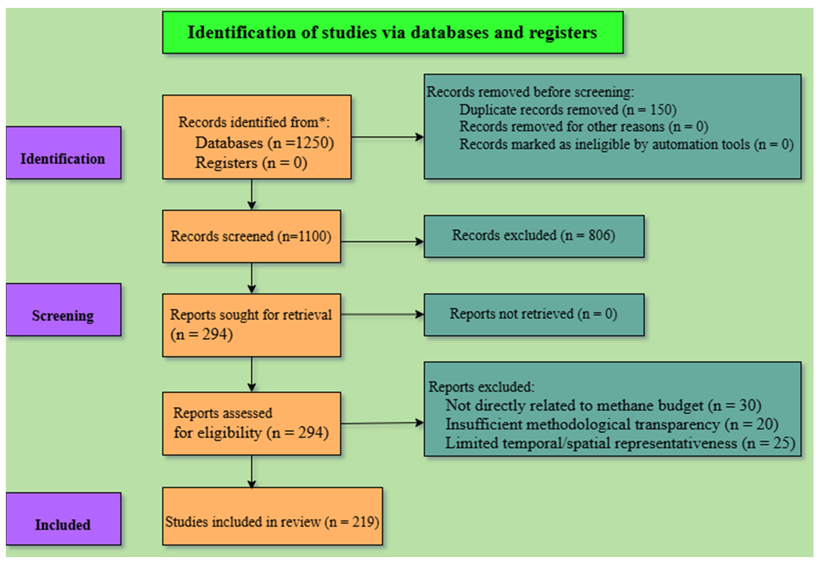
A comprehensive literature search initially identified more than 1250 publications using a combination of keywords related to CH₄ budget estimation, including “methane budget,” “top-down inversion,” “bottom-up inventory,” “integrated methane modeling,” and “remote sensing methane.” The search was conducted across major scientific databases, including Web of Science, Scopus, and Google Scholar, and covered the period from 1990 to 2025, capturing both foundational studies and recent advances in methane research.

After removing duplicate records and screening titles and abstracts for relevance, 294 studies were retained for further evaluation. A detailed full-text assessment was then conducted, resulting in the final selection of 219 research articles and review papers for in-depth analysis. The selected studies represent a broad range of spatial scales, including global assessments (e.g., multi-decadal methane budgets), regional analyses (e.g., North America, Europe, China, Arctic, and Monsoon Asia), and site-specific investigations (e.g., wetlands, rice paddies, fossil fuel systems, and landfills). The dataset also spans diverse temporal scales, from short-term observational campaigns (daily to seasonal) to long-term studies covering multiple decades.

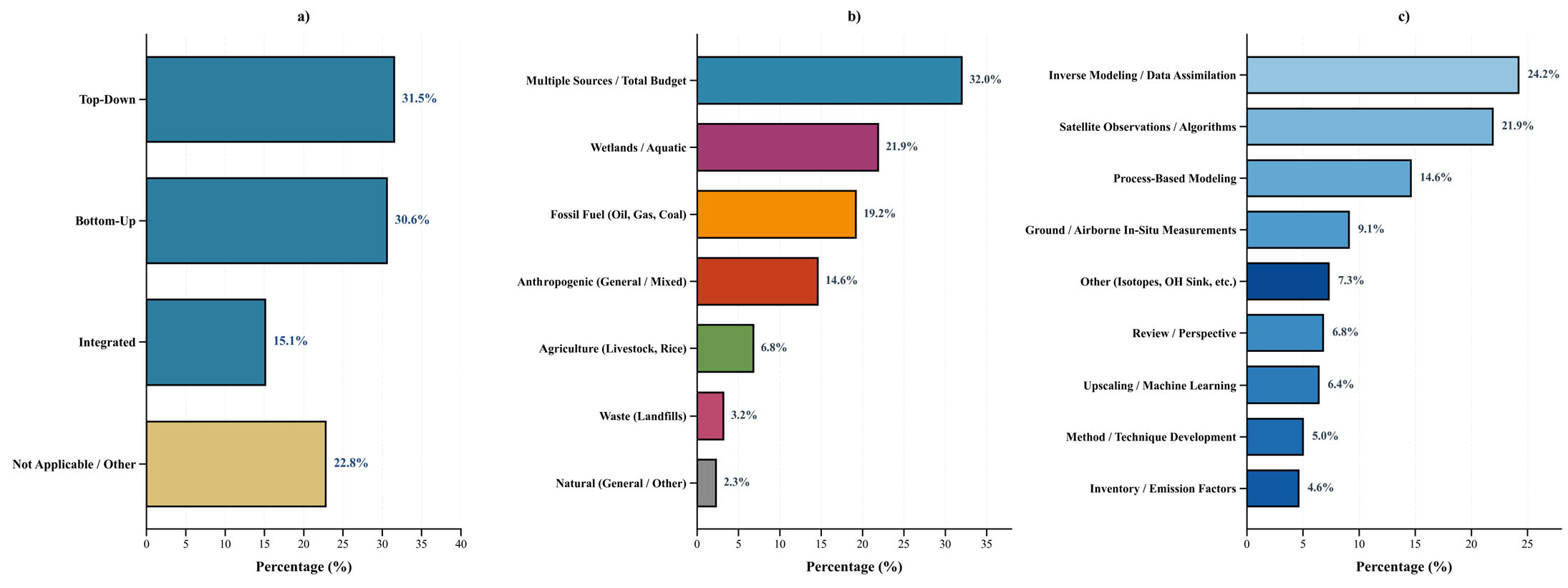
The inclusion criteria focused on studies that (i) quantified methane emissions and/or sinks, (ii) applied top-down, bottom-up, or integrated approaches, and (iii) reported quantitative estimates with clearly defined methodologies and uncertainties. Additional considerations included spatial and temporal resolution, as well as sectoral coverage of key methane sources, including wetlands, agriculture, fossil fuels, waste, and natural sinks. Studies were excluded if they lacked methodological transparency, did not directly address methane budget estimation, or had limited temporal (<1 year) or spatial representativeness, thereby restricting broader applicability. The overall selection process is summarized in Figure 1 and Figure 2.

This study adheres to the PRISMA 2020 guidelines [28]. A completed PRISMA checklist is provided in the Supplementary Materials. This review was not registered in a formal systematic review database.

3. Sources and Sinks of the CH4 Budget

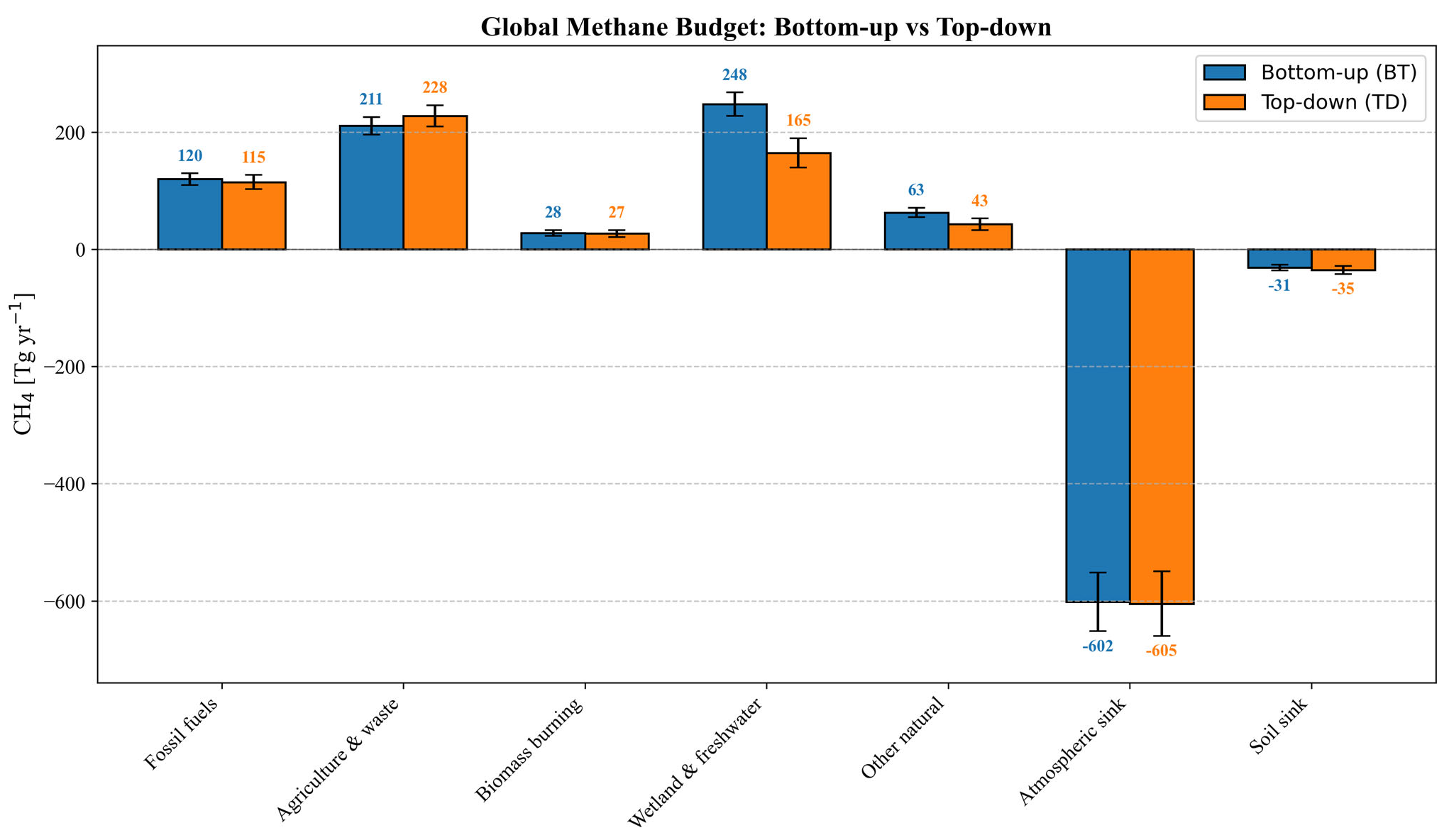
Methane emissions arise from natural sources, such as wetlands and aquatic ecosystems, and from anthropogenic sources, including agriculture, livestock farming, fossil fuel use, and biomass burning (Figure 3). A range of smaller sources, such as oceans and termites, also contribute [7]. The interplay among these CH₄ sources and sinks is crucial for determining the global CH₄ budget and understanding climate feedback mechanisms.

3.1. Anthropogenic Sources

Methane (CH₄) emissions originate from various anthropogenic sources, with agriculture the most significant contributor, accounting for approximately 51.24% to 62.12% of total emissions. Key agricultural contributors include enteric fermentation from ruminant livestock (39%), manure management through anaerobic decomposition (20%), rice cultivation (30%), and seasonal biomass burning (11%) [8,13,14,15]. In addition to agriculture, fossil fuel-related activities, such as coal mining, oil and gas extraction, and combustion processes, account for about 23.87% to 37.91% of total methane emissions. Urban sources, such as landfills and wastewater management, also play a significant role, accounting for 6% to 20% from landfills and 2% to 9% from wastewater, totaling 8% to 29% of total anthropogenic methane emissions [8,9,10,11,12].

3.2. Natural Sources

A total of 35% to 50% of methane (CH₄) emissions worldwide come from natural sources, with wetlands contributing 20% to 30% (115–230 Tg CH₄ annually) [19,20,21,22,23]. Oceans and coastal regions supply roughly 5% (29 Tg CH₄), whereas freshwater bodies contribute 8% to 10% (46–58 Tg CH₄). Geothermal activity and geological emissions from mud volcanoes contribute about 8% (45–53 Tg CH₄) [16,17,18]. An estimated 431.3 ± 87.9 Tg CH₄ is released annually by aquatic ecosystems, accounting for 53% of global emissions. Rivers, lakes, wetlands, and rice paddies are examples of inland water sources that emit approximately 398.1 ± 79.4 Tg CH₄, whereas coastal and open-ocean zones contribute approximately 33.2 ± 37.6 Tg CH₄ [23,24,25]. Temperature, water table depth, microbial populations, and salinity, especially in the summer and fall, are important determinants of methane emissions from the aquatic ecosystems [20,26,27]. Despite the challenges they pose [19,20,29,30], precise estimation techniques are crucial for understanding the contribution of these emissions to climate change [2]. Accurately assessing the contribution of methane emissions to climate change requires improved methods. Mitigation strategies to reduce methane’s impact on global warming can be informed by a better understanding of the factors driving its release.

3.3. Methane Sinks

Methane sinks are mechanisms that remove methane (CH₄) from the atmosphere (Figure 3), primarily through reactions with hydroxyl radicals (OH) and methane uptake by soils and wetlands. The reaction with OH accounts for approximately 80–90% of atmospheric methane removal [31]. However, the strength of this sink is uncertain due to variability in OH concentrations, influenced by human activities such as nitrogen oxides (NOₓ) and carbon monoxide (CO) emissions, which interact to significantly modify OH levels [32,33].

Soils, particularly in upland ecosystems, also play a crucial role, accounting for about 30–40 Tg yr⁻¹ of global methane uptake. Their effectiveness as a sink is highly variable and depends on factors such as soil moisture, temperature, nitrogen deposition, and microbial dynamics, which are often oversimplified in global models [34,35,36,37].

Wetlands present a dual role as both sources and sinks of methane. Traditionally seen as significant methane emitters, wetlands also oxidize methane via methanotrophic bacteria, which convert CH₄ into CO₂. The efficiency of this process depends on factors such as oxygen diffusion, redox potential, and environmental conditions, including water table fluctuations and temperature [38,39]. Recent studies indicate that tropical wetlands can enhance methane uptake under specific hydrological and biogeochemical conditions, underscoring their dynamic role in methane cycling and their potential to offset some methane emissions [38].

4. CH₄ Budget Estimation Approaches

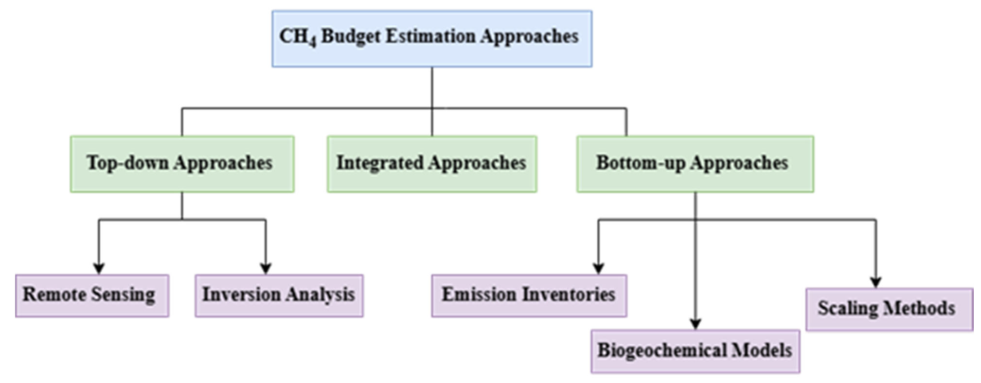
Methane budget estimation approaches can be broadly classified into top-down, bottom-up, and Integrated (combining top-down and bottom-up approaches), each with distinct methodologies and challenges (Figure 4) [29,40,41,42,43,44,45,46].

Applying a single-based approach relies solely on either top-down or bottom-up techniques, such as using atmospheric inversion models based exclusively on satellite data or aggregating emission factors without incorporating atmospheric observations. While informative, they are constrained by the limitations of their respective methodologies, such as difficulties in source attribution in top-down methods and potential underestimation of emissions, particularly from diffuse or poorly monitored sources, such as agriculture and wetlands, in bottom-up methods [16,47,48].

An integrated approach, on the other hand, combines top-down and bottom-up techniques to enhance the accuracy and reliability of methane budget estimates. By reconciling atmospheric measurements with detailed source inventories, integrated methods provide a more comprehensive understanding of methane emissions, enabling the identification of discrepancies, refinement of emission factors, and improvement of atmospheric models, ultimately leading to more accurate and actionable methane budgets [22,49,50,51].

4.1. Top-Down Approaches

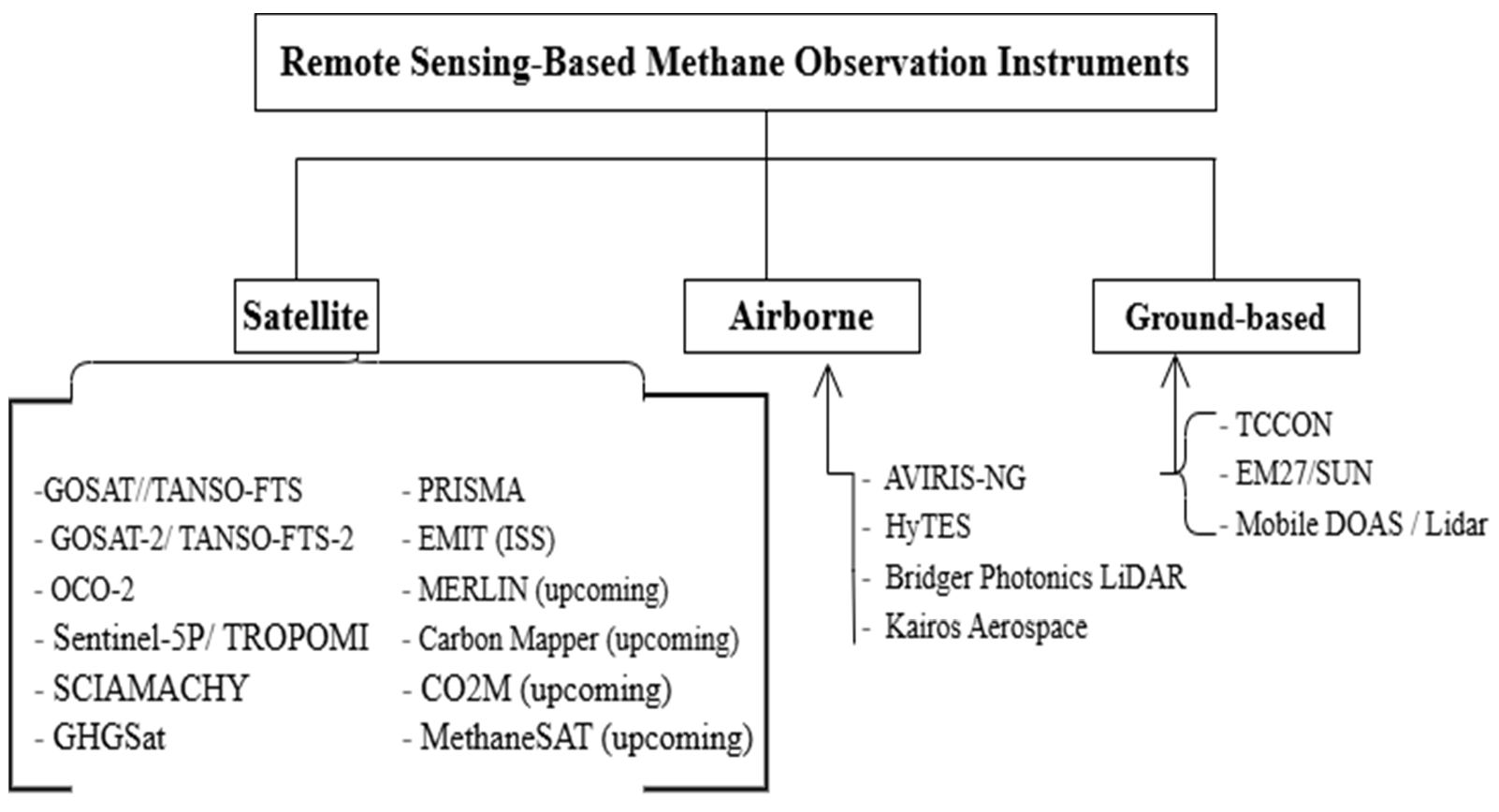
Top-down approaches estimate methane emissions by analyzing atmospheric CH₄ concentrations using models that simulate atmospheric transport from emission sources to observation points [13,29,30,31]. This approach infers surface emissions from atmospheric observations, using atmospheric transport models and inverse modeling techniques. It begins by examining the overall behavior of the methane system and deducing surface fluxes that contribute to observed concentrations [31]. Remote sensing technologies (Figure 5 and Table 1) are essential for acquiring these observations [29,32,33,34]. Top-down approaches yield observationally constrained, spatially integrated fluxes, providing a direct measure of emissions entering the atmosphere [30]. They excel at pinpointing emission hot spots and validating national greenhouse gas emission reports [29,35]. However, while the Top-down approach has notable strengths, it often lacks the specificity needed to allocate emissions to distinct sectors or source types without further constraints [13,30].

4.1.1. Remote Sensing Technologies

Remote sensing technologies are crucial for identifying, geolocating, and quantifying near-surface methane emissions. These technologies operate from land-based, airborne, and satellite platforms, each offering distinctive features essential for top-down methane estimation (Figure 5). These tools enable observations across a range of spatial and temporal scales, vital for understanding global methane sources and sinks [29].

Satellite instruments are crucial for their broad spatial coverage and for repeated observations of atmospheric methane (Figure 5 and Table 1). These techniques measure column-averaged dry-air mole fractions (XCH₄) [29] using shortwave infrared (SWIR) and thermal infrared (TIR) spectral ranges, key to global assessments of methane emissions [36,37].

Satellite instrumentation offers several benefits for the Top-down approach of methane budget estimation, including global coverage and frequent revisit cycles, which are essential for trend monitoring [15,29,36]. High-resolution sensors such as TROPOMI (Tropospheric Monitoring Instrument) enable the detection of emission hotspots and help refine source locations within models. Additionally, satellite data reduces global methane estimate uncertainty to about 5–7%, outperforming traditional bottom-up approaches. GOSAT (Greenhouse Gas Observing Satellite) data are also useful for tracking OH concentrations, which are critical for modeling methane’s atmospheric lifetime [38].

However, Satellite instruments also have limitations [29], including atmospheric conditions such as cloud cover and aerosols, which can hinder observations, leading to data gaps and biases. SWIR instruments, which rely on reflected sunlight, are less sensitive to near-surface methane, especially in low-reflectance or high-aerosol areas. There is a trade-off between high spatial resolution and frequent revisit times, impacting the detection of rapid or small, transient emissions. The accuracy of methane measurements relies on retrieval algorithms [39] that can be influenced by surface albedo, temperature, and water vapor. Future missions like MERLIN, Carbon Mapper, CO2M, and MethaneSAT aim to enhance detection capabilities, with MethaneSAT specifically targeting oil and gas infrastructure [37,40,41].

Airborne instruments, mounted on aircraft, offer flexible deployment and superior spatial resolution for detecting localized sources compared to satellites [38,42,43], but they have more limited spatial and temporal coverage (Table 1). Airborne instruments for Top-down estimation offer high spatial resolution and flexibility, enabling precise identification of emission sources that lower-resolution satellite data might miss. They are ideal for targeted campaigns focused on specific emission events or model validation, especially near known industrial sites [44,45]. Flying at lower altitudes improves their sensitivity to near-surface emissions, leading to more accurate methane measurements. However, airborne instruments face limitations [29,45,46], including restricted spatial and temporal coverage due to operational costs and logistical challenges, making them less suitable for continuous global monitoring. Their expense also limits the frequency and extent of deployments. Like satellites, airborne sensors are affected by weather conditions, especially cloud cover, which can reduce measurement quality.

Ground-based instruments are essential for precise, localized measurements needed for source characterization and the calibration of satellite and airborne data [29]. Ground-based instruments use Fourier Transform Spectrometers to collect long-term, accurate data on greenhouse gas concentrations, including methane, and Mobile DOAS (Differential Optical Absorption Spectroscopy) and LiDAR technologies are used for vehicle-mounted surveys to measure methane absorption and detect methane plumes, respectively [47,48]. These technologies set the gold standard for atmospheric monitoring accuracy and are crucial for calibrating and validating satellite data, providing continuous, long-term records of methane concentrations, and enabling detailed in situ source characterization [49]. Nevertheless, they face significant limitations, including limited spatial coverage, an inability to provide a broad overview of emissions, and high maintenance and operational costs [48].

Based on spatial resolution, detection thresholds, and application scales, remote sensing-based methods for methane emission estimation can be broadly categorized into area flux mappers and point-source imagers.

4.1.2. Area Flux Mappers

Area flux mappers are satellite instruments that measure methane emissions across various scales, from regional to global, with exceptional accuracy (often below 1%), and provide long-term monitoring [50,51,52]. They effectively evaluate methane emissions from large sources such as wetlands, agriculture, and fossil fuels, excelling in trend analysis and emission validation despite generally lower spatial resolution. Examples include GOSAT and TROPOMI [52] (Table 1). GOSAT, active since 2009, has played a key role in documenting methane concentrations and trends at national and regional levels, especially over wetlands and agricultural areas [33,51,53,54]. TROPOMI, launched in 2018 on the Sentinel-5P satellite, provides daily global coverage with a spatial resolution of up to 7 × 5.5 km², enabling the detection of major methane plumes and previously unknown emission hotspots, thereby improving regional emission assessments [26,55,56].

Despite these performances, area flux mappers also face limitations. One major challenge is the spatial resolution, which is often too coarse to detect small, localized emission sources. For example, the GOSAT has a pixel size of 10 km², making it unsuitable for pinpointing individual point sources [50]. Additionally, the accuracy of methane emission estimates from these sensors heavily depends on the retrieval algorithms used. Physical models and proxy-based methods, such as the carbon dioxide proxy method, can introduce uncertainties in quantification [57,58]. Furthermore, these methods often require multi-year averaging to achieve the precision needed for regional estimates, which limits their usefulness for near-real-time monitoring [50,51].

4.1.3. Point Source Imagers

Point-source imagers are specialized instruments designed to detect and quantify methane (CH₄) emissions from specific anthropogenic sources, including oil and gas infrastructure, landfills, and industrial facilities. They feature ultra-high spatial resolution, typically less than 60 m, allowing for precise localization and attribution of emissions to individual sources [37,59]. Notable examples include the GHGSat (Greenhouse Gas Satellite) Constellation and PRISMA. The GHGSat Constellation, a commercial satellite system with 25-m resolution, is widely used for high-precision CH₄ emissions detection, capable of detecting emissions at a threshold of 100 kg/h [50,60,61,62]. It employs hyperspectral imaging and spectroscopic retrieval techniques, significantly enhancing methane quantification and monitoring efforts [61,63]. PRISMA, developed by the Italian Space Agency, integrates high-spectral- and spatial-resolution imaging, which aids in detecting and quantifying CH₄ plumes, particularly across diverse surface environments [57,59,64,65].

Despite their advantages in spatial accuracy, point-source imagers face challenges, including higher detection thresholds that limit their ability to identify lower-magnitude emissions [50,66]. Their effectiveness can also be compromised by surface heterogeneity and temporal variability, leading to uncertainties in CH₄ flux retrieval and quantification [50,54,60]. Moreover, their emphasis on spatial detail often comes at the expense of temporal coverage, reducing their suitability for continuous monitoring [67]. Thus, while these instruments prove highly effective in targeted monitoring and verification, their limitations must be considered in broader emissions assessment contexts.

Table 1. Satellite, Airborne, and Ground-based instruments for atmospheric methane observation classified by platform, instrument, spectral range, and spatial/temporal resolution.

Instrument/Mission	Spectral Range	Spatial Resolution	Temporal Resolution	Launched Year	Type	Application	Remarks	Source
GOSAT/TANSO-FTS	SWIR/TIR	~10.5 km	3-day	2009	Passive	Global mapping, Emission inventory	High spectral resolution	[48,68]
GOSAT-2/TANSO-FTS-2	SWIR/TIR	10.5 km	3-day	2018	Passive	Global mapping, Emission inventory	Enhanced coverage and resolution	[69]
OCO-2	SWIR	1.29 × 2.25 km	~16-day	2014	Passive	Global mapping, Emission inventory	useful for synergy	[70]
Sentinel-5P/TROPOMI	SWIR, UV/VIS	7 × 7 km (initial), 5.5 × 7 km (after 2019)	Daily	2018	Passive	Global mapping, Emission inventory	Moderate resolution, wide swath	[71]
SCIAMACHY	NIR/SWIR	~60 × 30 km	6-day	2002–2012	Passive	Global mapping	First, to provide CH4 from space	[72]
GHGSat	SWIR	~25 m	2–3 weeks	2016	Passive	Plume Detection, Emission Inventory	Commercial, high-res, focused on point sources	[73]
PRISMA	VNIR-SWIR	30 m	~29-day	2019	Passive	Plume Detection (Experimental)	Hyperspectral, not optimized for CH4	[74]
EMIT (ISS)	SWIR	60 m	Targeted (not continuous)	2022	Passive	Plume Detection (targeted)	CH4 plumes detectable	[75]
MERLIN (upcoming)	IPDA Lidar	~50 m (along track)	16-day	upcoming	Active	Global Mapping, Emission Inventory	First spaceborne CH4 lidar mission	[76]
Carbon Mapper (upcoming)	SWIR (Hyperspectral)	30 m	Biweekly (planned)	upcoming	Passive	Plume Detection, Emission Inventory	Precise CH4 mapping	[77]
CO2M (upcoming)	SWIR/NIR	<5 km	Daily	upcoming	Passive	Global Mapping, Emission Inventory	EU mission for anthropogenic emissions	[78]
MethaneSAT	SWIR	1–3 km (regional), ~100 m (target mode)	3–7 days	2024	Passive	Plume Detection, Emission Inventory	Targeted for high emitters	[79]
AVIRIS-NG (airborne)	SWIR (Hyperspectral)	~3–5 m	Campaign-based	2012	Passive	Plume detection	Precise plume mapping	[80]
HyTES	TIR	5 m	Campaign-based	2012	Passive	Plume detection [81,82]	Thermal hyperspectral for hot spots (airborne)	[81,82]
Bridger Photonics LiDAR (airborne)	Lidar	~1–5 m	Campaign-based	2019	Active	Plume detection	Direct plume quantification	[83]
Kairos Aerospace	IR (TIR)	~5 m	Campaign-based	2016	Passive	Plume detection	Imaging spectrometer for emissions	[84]
TCCON	SWIR	N/A (column)	Continuous		Passive	Emission Inventory	Calibration/reference network	[48]
EM27/SUN	SWIR	N/A (column)	Continuous/campaign		Passive	Emission Inventory	Portable, widely deployed	[85]
Mobile DOAS/Lidar	UV-VIS or IR	~meters	Campaign-based	2022	Active/Passive	Emission Inventory, plume detection	Vehicle or fixed, used for verification (airborne)	[86]

Table 1. Satellite, Airborne, and Ground-based instruments for atmospheric methane observation classified by platform, instrument, spectral range, and spatial/temporal resolution.

Instrument/Mission	Spectral Range	Spatial Resolution	Temporal Resolution	Launched Year	Type	Application	Remarks	Source
GOSAT/TANSO-FTS	SWIR/TIR	~10.5 km	3-day	2009	Passive	Global mapping, Emission inventory	High spectral resolution	[48,68]
GOSAT-2/TANSO-FTS-2	SWIR/TIR	10.5 km	3-day	2018	Passive	Global mapping, Emission inventory	Enhanced coverage and resolution	[69]
OCO-2	SWIR	1.29 × 2.25 km	~16-day	2014	Passive	Global mapping, Emission inventory	useful for synergy	[70]
Sentinel-5P/TROPOMI	SWIR, UV/VIS	7 × 7 km (initial), 5.5 × 7 km (after 2019)	Daily	2018	Passive	Global mapping, Emission inventory	Moderate resolution, wide swath	[71]
SCIAMACHY	NIR/SWIR	~60 × 30 km	6-day	2002–2012	Passive	Global mapping	First, to provide CH4 from space	[72]
GHGSat	SWIR	~25 m	2–3 weeks	2016	Passive	Plume Detection, Emission Inventory	Commercial, high-res, focused on point sources	[73]
PRISMA	VNIR-SWIR	30 m	~29-day	2019	Passive	Plume Detection (Experimental)	Hyperspectral, not optimized for CH4	[74]
EMIT (ISS)	SWIR	60 m	Targeted (not continuous)	2022	Passive	Plume Detection (targeted)	CH4 plumes detectable	[75]
MERLIN (upcoming)	IPDA Lidar	~50 m (along track)	16-day	upcoming	Active	Global Mapping, Emission Inventory	First spaceborne CH4 lidar mission	[76]
Carbon Mapper (upcoming)	SWIR (Hyperspectral)	30 m	Biweekly (planned)	upcoming	Passive	Plume Detection, Emission Inventory	Precise CH4 mapping	[77]
CO2M (upcoming)	SWIR/NIR	<5 km	Daily	upcoming	Passive	Global Mapping, Emission Inventory	EU mission for anthropogenic emissions	[78]
MethaneSAT	SWIR	1–3 km (regional), ~100 m (target mode)	3–7 days	2024	Passive	Plume Detection, Emission Inventory	Targeted for high emitters	[79]
AVIRIS-NG (airborne)	SWIR (Hyperspectral)	~3–5 m	Campaign-based	2012	Passive	Plume detection	Precise plume mapping	[80]
HyTES	TIR	5 m	Campaign-based	2012	Passive	Plume detection [81,82]	Thermal hyperspectral for hot spots (airborne)	[81,82]
Bridger Photonics LiDAR (airborne)	Lidar	~1–5 m	Campaign-based	2019	Active	Plume detection	Direct plume quantification	[83]
Kairos Aerospace	IR (TIR)	~5 m	Campaign-based	2016	Passive	Plume detection	Imaging spectrometer for emissions	[84]
TCCON	SWIR	N/A (column)	Continuous		Passive	Emission Inventory	Calibration/reference network	[48]
EM27/SUN	SWIR	N/A (column)	Continuous/campaign		Passive	Emission Inventory	Portable, widely deployed	[85]
Mobile DOAS/Lidar	UV-VIS or IR	~meters	Campaign-based	2022	Active/Passive	Emission Inventory, plume detection	Vehicle or fixed, used for verification (airborne)	[86]

In general, recent advances in remote sensing technologies have begun to address several limitations of traditional methane monitoring methods by improving spatial and temporal resolution, advancing algorithms, and integrating sensors. Emerging satellite missions, such as the Environmental Defence Fund (EDF) mission for methane monitoring (MethaneSAT) and GeoCarb, are designed to provide higher spatial resolution (ranging from 1 to 10 km²) along with increased revisit frequencies, enabling more precise and consistent monitoring of methane emissions [50,51].

The integration of machine learning (ML) and artificial intelligence (AI) techniques, such as convolutional neural networks (CNNs) and support vector machines (SVMs), has significantly enhanced the ability to detect and quantify methane plumes from satellite data. These methods have been successfully used with instruments such as TROPOMI for the automatic identification of methane super-emitters [67]. The combined use of multi-sensor observations (integrating data from area flux mappers and point source imagers) has increased the accuracy of emission quantification. For example, TROPOMI can be used for broad-scale plume detection, which can then be analyzed at finer spatial resolutions using targeted sensors such as GHGSat or PRISMA [67].

Integrating satellite observations with advanced analytical frameworks helps address gaps in historical observational coverage, thereby enhancing global methane budget assessments. A study using TROPOMI satellite data has significantly refined methane budget estimates by offering high-resolution, near-global information. However, discrepancies still exist in the rate of methane flux increase, mainly due to underestimated emissions from tropical wetlands [10].

TROPOMI observations have shown that emissions from tropical wetlands are higher than previously estimated, with a posteriori increases of up to 25 Tg CH4 yr⁻¹, and tropical wetlands now contribute about 70% of the total. These observations also highlight the importance of regional hydrology in affecting methane emissions [10]. GOSAT data have been used to evaluate how well models like WetCHARTs and JULES simulate the seasonal cycle of methane emissions. Although these models generally do a good job, they often underestimate the emission amplitude in specific areas, such as the North Tropics [54,87].

Aircraft campaigns, such as SEAC4RS (Studies of Emissions and Atmospheric Composition, Clouds, and Climate Coupling by Regional Surveys), play a complementary role in measuring methane concentrations in the boundary layer. They provide in situ data in regions with limited satellite coverage and offer detailed vertical profiles, which are valuable for validating satellite data and enhancing our understanding of the methane cycle [88]. A comparison study between aircraft/airborne measurements and WRF-Chem model simulations to quantify methane emissions in the US shows that top-down flux estimates, compared to bottom-up predictions, vary by source type, and Southern US wetland emissions were overestimated by the WetCHARTs inventory [42].

4.2. Perform Inversion Analysis

In many scientific fields, especially atmospheric chemistry and Earth system research, inversion analysis, also called inverse modeling, is a key method for determining unknown source parameters or underlying processes from observed effects [89,90,91]. The main idea is to use a forward model that explains the relationship between observations (such as atmospheric methane levels) and unknown parameters (such as methane emissions). Then, the inverse problem seeks the source parameters that best fit the observed data, often considering prior information about these parameters [89,90,91,92]. This approach is crucial for measuring emissions across large spatial and temporal scales that are difficult to measure directly [89,91].

Inversion analysis uses Bayesian inference to combine prior source estimates and uncertainties with observational data and atmospheric transport models, leading to improved posterior estimates [13]. It involves a forward model, usually an atmospheric chemistry-transport model (CTM), to simulate methane transport, mixing, and transformation, which are then compared with observed concentrations [91]. The inverse problem aims to minimize a cost function measuring the difference between model predictions and observations while penalizing deviations from prior estimates [13,91].

Key components include prior information, observations, a forward model (observation operator), a cost function, and an optimization algorithm.

• Prior Information: initial source estimates and uncertainties from sources like process-based models for natural emissions (wetlands) and activity data for human sources (agriculture, landfills) [13,93,94].
• Observations: atmospheric measurements from ground sensors or satellites (e.g., GOSAT, TROPOMI, AIRS), each with uncertainties [26,31].
• Forward Model (Observation Operator): a CTM (like MOZART-4 or CMAQ) linking source parameters to observed concentrations through atmospheric processes [95].
• Cost Function: quantifies mismatch between model and data, considering deviations from priors, weighted by errors [13].
• Optimization Algorithm: techniques that iteratively adjust source parameters to minimize the cost function [91].

Inversion analysis for methane budget estimates requires atmospheric methane concentration observations for model validation and to understand local variations [26,31]. It requires prior emission inventories from natural sources, such as wetlands and permafrost, as well as from anthropogenic sources, such as agriculture and fossil fuels, providing context for the inverse problem [96,97,98,99,100,101,102]. Additionally, meteorological data, including wind speed, temperature, humidity, and pressure, are vital for atmospheric transport models [91], along with atmospheric chemical information, particularly hydroxyl radical (OH) concentrations, which are essential for modeling methane’s atmospheric lifetime [15,103].

Methane inversion analysis employs several major techniques, each with distinct principles, strengths, and limitations. Some of the most commonly used inversion analysis techniques are as follows.

4.2.1. The Bayesian Inversion Techniques

Bayesian techniques provide a robust statistical framework for integrating prior information, such as EDGAR, with atmospheric observations to identify patterns across time and space and to improve estimates of methane fluxes [13,104]. This technique estimates the most likely source distribution by minimizing a cost function that balances fitting the observations and respecting prior beliefs, while accounting for uncertainties via error covariance matrices [104,105].

Historically, Bayesian inversions focused on broad annual and decadal methane budgets but have evolved to support higher temporal and spatial resolutions and more complex error structures [91,96].

They now incorporate various observational datasets, including satellite and ground-based data, and use modern ensemble-based methods to better assess uncertainties [13]. These techniques are especially good at quantifying uncertainty and can potentially decrease prior flux estimates by 30–60%, depending on data quality and coverage [13].

However, their success relies heavily on accurately defining prior uncertainties and observation covariances, making them more vulnerable to sparse data and thereby more difficult to identify sources.

The study on performance in Bayesian inversion techniques for estimating methane budgets highlights the complex relationships among resolution, uncertainty, and information content, which are affected by observational capabilities and model physics. Key findings show a hierarchical pattern in inversion performance, related to the choice of spatial and temporal scales. At the global level, using a 1° × 1° resolution and monthly data aggregation, Bayesian inversions produce minimal relative uncertainties (±5%) due to strong observational constraints from satellite data. This results in sector-specific methane emission estimates: agricultural and fire emissions are 227 ± 19 Tg CH₄/yr, waste emissions are 50 ± 7 Tg CH₄/yr, anthropogenic fossil emissions are 82 ± 12 Tg CH₄/yr, and natural emissions are 180 ± 10 Tg CH₄/yr [2,105]. However, this level of precision is limited by significant aggregation bias, which masks the heterogeneity of emissions within sub-grid scales [105,106].

Bayesian inversion is also shown to be highly effective at the regional scale for identifying discrepancies between reported national inventories and atmospheric constraints. For instance, it reveals that methane emissions in China are approximately 21% higher than reported, particularly from livestock, waste, and rice paddies [25]. This is different from bottom-up inventories, which tend to underestimate emissions from diffuse agricultural sources. In India, Bayesian inversion captures increased emissions from rice paddies and wetlands during the summer monsoon, a seasonal dynamic that inventory methods do not account for [10]. In the United States, inversions also reveal that landfills and the oil and gas industry make significant contributions, often exceeding those reported by the government [27]. Bayesian inversion not only identifies these underreported sources by comparing atmospheric observations with existing knowledge, but also provides policymakers with more useful information by providing confidence intervals.

However, the effectiveness of regional-scale inversions has limitations. At higher spatial resolutions (0.1–0.5° with weekly updates), uncertainties increase, mainly because inversion models depend heavily on the accuracy of prior emission fields and atmospheric transport simulations, leading to potential posterior uncertainties of 20–50% under less ideal conditions [106,107]. This problem is especially significant in areas with complex emission patterns, such as Shanxi Province’s coal-mining regions and agriculture-intensive rice cultivation zones, where emissions vary widely and are difficult to represent accurately in prior inventories [108,109].

Additionally, several structural issues remain within the Bayesian inversion method. Systematic biases in prior emission inventories can distort posterior estimates if not properly constrained. Inaccuracies in atmospheric transport models, particularly in regions with complex terrain or limited observational coverage, further complicate the estimation of emission fluxes. Moreover, observational limitations, such as data gaps in satellite methane retrievals due to cloud cover and sensor restrictions, further increase uncertainty [104,107]. These challenges highlight the need for continuous improvements in inversion techniques, better atmospheric transport modeling, and expanded observational networks to increase the reliability of methane emission evaluations.

Future advancements to enhance the applicability of Bayesian inversion across different spatial and temporal scales, such as improving the coverage and observation of methane data, refining prior inventories, and integrating additional tracers (incorporating multi-tracer approaches, such as ethane and carbon monoxide), are very vital for strengthening the accuracy of inversion-based estimates, reducing biases and refining model outputs, and providing additional constraints on methane emissions and improving source attribution [104,110,111].

4.2.2. Four-Dimensional Variational (4D-Var) Data Assimilation

The 4D-Var method is one of the most advanced approaches for analyzing methane budgets [112]. It offers clear advantages over other methods, such as Bayesian and ensemble Kalman filter (EnKF) techniques [113]. 4D-Var systematically recalibrates previous emissions to match observations by integrating satellite, ground-based, and aircraft data with atmospheric transport models [112]. This enhances the spatial and temporal resolution of methane fluxes [114]. A key feature that makes 4D-Var exceptional is its use of an adjoint model, which rapidly propagates sensitivities backwards in time and facilitates large-scale optimization. This method enforces more stringent limits on sources compared to other approaches [33,115,116].

Comparative tests indicate that 4D-Var offers enhanced resolution. For example, the FLEXVAR system, which operates at a 7 km resolution, detects emission hotspots more precisely than coarser global models, such as TM5-4DVAR (1° × 1°) [114]. Meanwhile, global systems based on ECMWF’s IFS with 4D-Var have shown notable increases in emissions in regions such as China, India, and Indonesia, primarily due to microbial activity [117]. Furthermore, 4D-Var has proven highly effective in utilizing satellite data from instruments such as GOSAT and SCIAMACHY. It has reduced biases and improved alignment with surface measurements, aiding in correcting underestimates of fossil fuel emissions in North America and in reassessing tropical methane sources [118,119]. These findings differ from traditional bottom-up inventories, which often do not display this level of variability.

Although 4D-Var has some advantages, it also has notable drawbacks. It is vulnerable to assumptions about model error covariance, and implementations with low resolution can hide small-scale sources [1,107,120]. Additionally, retrieval biases and limited coverage, particularly in tropical regions, continue to pose significant challenges that compromise the accuracy of methane estimates [58,120,121]. Nonetheless, compared to alternative methods, 4D-Var consistently demonstrates a superior ability to integrate diverse data streams, enhance spatial resolution, and reduce uncertainties in global and regional methane budgets.

4.2.3. Kalman Filter Techniques

Kalman Filter (KF) approaches of inversion analysis are an essential technique in methane budget analysis, as they are able to combine observations from multiple sources while carefully managing uncertainties. By integrating remote sensing datasets and outputs from air transport models, KF methods enhance the accuracy of emission estimates and improve the spatial and temporal detail of methane budgets [122,123,124,125]. Different versions of KF have been developed to address the unique challenges of methane inversion modeling, such as the Extended Kalman Filter (EKF), Ensemble Kalman Filter (EnKF), Unscented Kalman Filter (UKF), and Local Ensemble Transform Kalman Filter (LETKF), each addressing specific limitations. All these KF techniques work together to offer versatile and powerful tools for more precise methane budget estimation across different times and locations. They balance accuracy, computational feasibility, and the capacity to model nonlinear system dynamics.

The Extended Kalman Filter (EKF) works by linearizing around the current state and then adapting the technique for nonlinear systems, which enables it to perform well in environments that are only slightly nonlinear [124]. The Ensemble Kalman Filter (EnKF) has been enhanced to mitigate the EKF’s computational limitations by utilizing ensembles to represent uncertainties, making it particularly suitable for large atmospheric models [125]. The Unscented Kalman Filter (UKF) advances this further by employing deterministic sampling to capture nonlinear dynamics better, resulting in more accurate estimates without linearization [123]. The Local Ensemble Transform Kalman Filter (LETKF) enhances scalability and efficiency, functioning effectively in high-dimensional atmospheric systems while still providing reliable estimates of methane emissions [122].

4.2.4. Machine Learning-Based Inversions

Machine learning-based inversion techniques are now widely used to estimate methane budgets, leveraging increased computing power to improve predictive accuracy and reduce uncertainty in emission assessments [126,127,128,129,130]. This is due to their ability to dynamically combine datasets, identify nonlinear correlations, and better detect complex emission patterns than traditional inversion frameworks [131,132,133]. These methods are crucial for understanding methane’s role in climate change and mitigating its impact by improving inventories, identifying super-emitters, and enhancing the accuracy of national and regional emission estimates [129,134].

Among machine learning models, Logistic regression, artificial neural networks, and support vector regression exhibit elevated predictive accuracy, as indicated by substantial R² values. In contrast, random forest models provide a more robust understanding of biogeochemical processes by analyzing methane clumped-isotopologue distributions [129,130,134]. These developments highlight the potential of machine learning methodologies to enhance conventional methane budget calculations, particularly by overcoming the limitations of traditional inversion models.

Using a data-driven, flexible machine learning approach combined with a traditional inversion method (such as Bayesian, adjoint-based, or hybrid) helps reduce errors in parameterization and improves the efficiency of transport models in merging atmospheric observations with chemical transport models, thereby supporting CH₄ flow analysis at global, regional, and local levels [135,136]. Recent applications demonstrate this complementarity. For example, inverse analyses using the GEOS-Chem adjoint model, combined with Bayesian cost-function minimization, showed that bottom-up inventories for the U.S., Canada, and Mexico underestimated methane emissions by 20–41% from 2010 to 2017 when compared to satellite (GOSAT) and in situ (ObsPack) assimilation results [137]. Similarly, high-frequency eddy covariance flux measurements from the FLUXNET-CH₄ network [98] and comprehensive Bayesian uncertainty analyses highlight the importance of observational constraints [89].

However, machine learning techniques can further improve these results by extrapolating data from under-sampled regions, especially tropical wetlands, and by combining various temporal and spatial datasets. Direct field-based measurements, such as rice paddy studies in India [138], provide vital empirical data on methane fluxes; however, their regional focus and limited temporal coverage restrict their applicability at a global level. Machine learning demonstrates its strength here by integrating localized data into scalable models, improving the accuracy of global methane budget estimates, and showing how methane levels vary by location [127]. Overall, machine learning-based inversion methods enhance methane budget estimation by providing more precise predictions, reducing reliance on strict parameterizations, and operating effectively within standard inversion frameworks [126,128,129,130]. These techniques are particularly good at capturing nonlinear emission dynamics, scaling localized data to larger areas, and providing valuable insights for developing emission-reduction strategies [127,131].

4.3. Bottom-Up Approaches

The bottom-up approach to methane (CH₄) budget estimation quantifies emissions by combining activity data (such as livestock populations, rice paddies, landfills, or oil and gas infrastructure) with emission factors derived from inventories, process-based models, and field measurements, aligned with IPCC Tier 1–3 methods [5,17,21,98,138,139,140,141,142,143]. This sector-specific framework provides transparency and source-specific detail essential for mitigation planning [13,144]. However, the accuracy of bottom-up estimates varies widely across spatial and temporal scales, with global uncertainties typically ranging from ±20% to ±50% due to variability in emission factors, incomplete activity data, and difficulties in capturing super-emitters [106]. Compared with atmospheric inversion (top-down) methods, bottom-up estimates often underestimate emissions, especially in wetlands and aquatic systems. For instance, bottom-up estimates of wetland emissions range from 102 to 182 Tg CH₄ yr⁻¹, whereas top-down estimates range from 159 to 200 Tg CH₄ yr⁻¹, revealing ongoing discrepancies [22,23,99,145]. Global syntheses, such as the Global Methane Budget, identify wetlands, agriculture, and fossil fuels as the main sources, with wetlands as the largest natural source and the greatest source of uncertainty [9]. Sectoral analyses further demonstrate these limitations: oil and gas inventories often underreport emissions [20,146,147], landfill estimates can be underestimated by up to 200% [94,148], and rice cultivation emissions remain poorly constrained, ranging from 18 to 115 Tg CH₄ yr⁻¹ [93,109]. Despite these challenges, bottom-up inventories offer valuable insights into the relative contributions of different sectors and, when combined with top-down atmospheric observations, form the foundation for reconciling differences, reducing uncertainties, and increasing confidence in global methane budget assessments [8,94,105].

4.3.1. Process-Based Models

Process-based models are crucial for simulating methane (CH₄) fluxes across ecosystems such as wetlands, peatlands, rice paddies, and uplands, where emissions are driven by biogeochemical processes sensitive to climate variability, hydrology, and land-use change [149,150].

Wetlands alone make a disproportionate contribution to the global methane budget, with East Asia accounting for over 63% of natural CH₄ emissions [120]. To capture these dynamics, a variety of models have been developed, ranging from site-specific frameworks like DNDC, Walter–Heimann, PEATLAND-VU, PCMLCH4, SWAMP-CH4, and HPM to regional-scale models such as DAYCENT, TEM, ED2-M, and VISIT, and global systems including LPJ variants, CLM, ORCHIDEE-PEAT, and JSBACH [17,147,149,151,152,153,154,155,156,157,158,159,160,161]. Although these models share the common goal of quantifying methane fluxes, they differ significantly in scope, complexity, and application (Table 2).

These differences in design reflect the trade-off between mechanistic detail and computational feasibility. High-resolution frameworks such as CLM and ORCHIDEE-PEAT incorporate detailed soil carbon pools, microbial dynamics, and vegetation-mediated transport, achieving strong agreement with global observations (R² > 0.8) [153]. In contrast, simpler models like Walter–Heimann rely on empirical relationships between water table depth and temperature, yielding moderate accuracy (R² = 0.5–0.7) [154]. Hydrological drivers are consistently central: Wetland-DNDC and Paddy-DNDC explicitly simulate water table depth, accurately predicting paddy CH₄ fluxes with RMSE values of 0.1–0.5 g CH₄ m⁻² day⁻¹ [155]. Vegetation interactions are equally critical, with LPJmL and ED2-M showing that plant-mediated transport can contribute up to half of total emissions in vegetated peatlands [149,152,155,158]. These design choices determine not only accuracy but also the scales at which models can be applied.

The suitability of each model becomes clearer when considering applications across different spatial and temporal scales. Local models offer detailed mechanisms for site-specific studies but are limited in scalability. Regional models strike a balance between accuracy and computational efficiency, making them appropriate for landscape and basin-level simulations, where they contribute to national greenhouse gas inventories and mitigation strategies. Global models expand coverage to continental and global domains, often integrated into Earth System Models with grid resolutions of 0.5–2° [150,159]. Temporal resolutions range from daily to seasonal, allowing for the simulation of both short-term flux events and long-term ecological dynamics. For instance, TEM and DAYCENT effectively reproduce seasonal CH₄ cycles with R² values above 0.8 [155]. Therefore, the scale at which a model is applied is closely related to the complexity of model design.

Performance metrics further demonstrate differences in predictive ability. High-performing models such as CLM, ORCHIDEE-PEAT, DNDC, DAYCENT, and TEM achieve RMSE values below 0.5 g CH₄ m⁻² day⁻¹ and R² above 0.8 [153,155]. LPJmL outperforms LPJ-Bern, especially in hydrological parameters, with R² values of 0.7–0.9 [158,159]. Moderate-performing models such as PEATLAND-VU, HPM, VISIT, and JSBACH show RMSEs of 0.5–1.0 and R² of 0.6–0.7 [152,156,157]. Simpler models like Walter–Heimann, PCMLCH4, and SWAMP-CH4 are limited by their empirical design, with RMSEs near 1.5 [154]. Sensitivity analyses consistently highlight water table depth, soil temperature, and organic carbon as major sources of uncertainty, with fluxes changing by 20–30% under ±10 cm variations in water table depth and by 15–25% with pH shifts [153,162]. These results underscore the significance of hydrological and biogeochemical drivers across all scales.

Although high-fidelity models like CLM, ORCHIDEE-PEAT, DNDC, and ED2-M are especially effective for wetland ecosystems, their complexity demands substantial computational power and extensive input data, which may not be available in data-poor regions, leading to regional uncertainties of 20–50%. Additionally, dynamic processes such as transient wet–dry cycles, redox fluctuations, permafrost thaw, and hydrological regime shifts are still poorly represented [153,163]. Recent advances, including prognostic water-table-depth schemes in ORCHIDEE-PEAT and CLM, integration of satellite data like SMAP soil moisture, and ensemble modeling frameworks, have enhanced hydrological accuracy and decreased uncertainty in global CH₄ budgets by 10–15% [152,164]. These developments show progress in balancing mechanistic accuracy with scalability.

In summary, process-based models show a clear trade-off between accuracy and scalability. Local models offer the mechanistic detail needed for ecological research, regional models balance detail with wider applicability, and global models provide the scalability crucial for policy-making. For ecological research, site-level models are essential for advancing mechanistic understanding of CH₄ dynamics, while regional models serve as platforms for scaling these insights across landscapes. For climate policy, global and regional models are vital because they produce scalable outputs aligned with international reporting frameworks and IPCC assessments. A tiered, hybrid approach, where local models validate processes, regional models expand findings, and global models project policy-relevant scenarios, offers the most comprehensive path forward. This integration, supported by machine learning and data assimilation, will help ensure that both ecological research and climate policy are driven by robust, multi-scale scientific evidence.

Table 2. Qualitative description of Process-based models.

Process based models	Model	Description	Accuracy (1–5)	Computational Demand (1–5)	Scalability (1–5)	Adaptability (1–5)	Source
	Local scale models: used for site-specific studies (e.g., a wetland, peatland, or rice field).
	DNDC (and sub-models like Wetland-DNDC, Paddy-DNDC)	Highly detailed and ideal for site-level applications with plot-scale data.	4.5	3.5	4.0	4.5	[165,166,167]
	Walter–Heimann Model	Developed for simulating CH4 emissions at the scale of specific wetland sites.	3.0	2.0	3.0	3.0	[168,169]
	PEATLAND-VU	Designed for high-resolution simulations in northern peatlands.	3.5	3.0	3.5	3.5	[157]
	PCMLCH4	Specifically developed for high-resolution, vertically stratified peatland simulations.	3.0	3.0	3.0	3.5	[170]
	SWAMP-CH4	Modular design suited for local soil and plant process interactions.	3.0	3.0	3.0	3.0	[127]
	HPM (Hydrogeomorphic Patch Model)	Patch-based model for small-scale boreal wetlands.	3.5	3.5	3.5	4.0	[156]
	Regional scale models: used for landscapes or basin-level simulations; can be upscaled or downscaled.
	DAYCENT/CENTURY	Originally for plot to landscape scale; has been adapted for regional applications.	4.5	3.5	4.5	4.5	[171]
	ED2-M	Scalable to landscape level, with vegetation structure and hydrology.	3.5	4.0	4.0	4.5	[149]
	TEM/Wetland-TEM	Applied in regional CH4 studies (e.g., Alaskan wetlands).	4.5	3.5	4.5	4.5	[155]
	VISIT	Applied across regions in East Asia and elsewhere for trace gas simulations.	3.5	3.0	4.0	3.5	[152]
	LPJ-Bern	Though derived from a global model, it has been used in regional CH4 studies.	3.5	3.5	5.0	3.5	[159]
	Global Scale models: capable of simulating CH4 emissions globally across diverse ecosystems [153,172]
	LPJ-wsl/LPJmL	Global dynamic vegetation model with CH4 emissions, land cover, and hydrology.	4.0	3.5	5.0	4.0	[158]
	CLM (Community Land Model)	Part of CESM; simulates global land-surface processes, including CH4.	4.5	4.5	5.0	4.5	[153,172]
	ORCHIDEE-PEAT	Modified for global peatland CH4 emissions.	4.5	4.5	5.0	4.5	[173]
	JSBACH	Land component of the MPI Earth System Model; includes global CH4 modules.	3.5	4.0	5.0	3.5	[150]

This qualitative analysis of process-based models is based on the accuracy, computational demand, scalability, and adaptability of the methane budget estimation process. Accuracy (Agreement with Observations): How well methane fluxes (e.g., g CH₄ m⁻² day⁻¹) match field measurements across various ecosystems (wetlands, peatlands, paddies, etc.). Scoring: −1: Poor (RMSE > 1.5 or R² < 0.3); 2: Low (RMSE 1.0–1.5 or R² 0.3–0.5); 3: Moderate (RMSE 0.5–1.0 or R² 0.5–0.7); 4: High (RMSE 0.2–0.5 or R² 0.7–0.9); 5: Excellent (RMSE < 0.2 or R² > 0.9) [123,124,125,146]. Computational Demand: Resources required (CPU time, memory in GB). Scoring Scale: −1: Very Low (<30 min, <0.5 GB); 2: Low (30 min⁻¹ h, 0.5–1 GB); 3: Moderate (1–6 h, 1–3 GB); 4: High (6–24 h, 3–10 GB); 5: Very High (>24 h, >10 GB) [135,147,148]. Scalability: Applicability from site (m²) to global (10⁶ km²) scales. Scoring Scale: −1: Site-only (<1 km²), 2: Local (1–100 km²); 3: Regional (100–10,000 km²); 4: Continental (10,000–1M km²); 5: Global (>1M km², seamless) [123,127,129,130,146]. Adaptability: Ease of integrating new processes or data. Scoring Scale: −1: Rigid (no updates possible); 2: Low (major rewrite needed); 3: Moderate (some updates, complex); 4: High (modular, moderate effort); 5: Excellent (highly modular, easy updates) [124,126,135].

Table 2. Qualitative description of Process-based models.

Process based models	Model	Description	Accuracy (1–5)	Computational Demand (1–5)	Scalability (1–5)	Adaptability (1–5)	Source
	Local scale models: used for site-specific studies (e.g., a wetland, peatland, or rice field).
	DNDC (and sub-models like Wetland-DNDC, Paddy-DNDC)	Highly detailed and ideal for site-level applications with plot-scale data.	4.5	3.5	4.0	4.5	[165,166,167]
	Walter–Heimann Model	Developed for simulating CH4 emissions at the scale of specific wetland sites.	3.0	2.0	3.0	3.0	[168,169]
	PEATLAND-VU	Designed for high-resolution simulations in northern peatlands.	3.5	3.0	3.5	3.5	[157]
	PCMLCH4	Specifically developed for high-resolution, vertically stratified peatland simulations.	3.0	3.0	3.0	3.5	[170]
	SWAMP-CH4	Modular design suited for local soil and plant process interactions.	3.0	3.0	3.0	3.0	[127]
	HPM (Hydrogeomorphic Patch Model)	Patch-based model for small-scale boreal wetlands.	3.5	3.5	3.5	4.0	[156]
	Regional scale models: used for landscapes or basin-level simulations; can be upscaled or downscaled.
	DAYCENT/CENTURY	Originally for plot to landscape scale; has been adapted for regional applications.	4.5	3.5	4.5	4.5	[171]
	ED2-M	Scalable to landscape level, with vegetation structure and hydrology.	3.5	4.0	4.0	4.5	[149]
	TEM/Wetland-TEM	Applied in regional CH4 studies (e.g., Alaskan wetlands).	4.5	3.5	4.5	4.5	[155]
	VISIT	Applied across regions in East Asia and elsewhere for trace gas simulations.	3.5	3.0	4.0	3.5	[152]
	LPJ-Bern	Though derived from a global model, it has been used in regional CH4 studies.	3.5	3.5	5.0	3.5	[159]
	Global Scale models: capable of simulating CH4 emissions globally across diverse ecosystems [153,172]
	LPJ-wsl/LPJmL	Global dynamic vegetation model with CH4 emissions, land cover, and hydrology.	4.0	3.5	5.0	4.0	[158]
	CLM (Community Land Model)	Part of CESM; simulates global land-surface processes, including CH4.	4.5	4.5	5.0	4.5	[153,172]
	ORCHIDEE-PEAT	Modified for global peatland CH4 emissions.	4.5	4.5	5.0	4.5	[173]
	JSBACH	Land component of the MPI Earth System Model; includes global CH4 modules.	3.5	4.0	5.0	3.5	[150]

This qualitative analysis of process-based models is based on the accuracy, computational demand, scalability, and adaptability of the methane budget estimation process. Accuracy (Agreement with Observations): How well methane fluxes (e.g., g CH₄ m⁻² day⁻¹) match field measurements across various ecosystems (wetlands, peatlands, paddies, etc.). Scoring: −1: Poor (RMSE > 1.5 or R² < 0.3); 2: Low (RMSE 1.0–1.5 or R² 0.3–0.5); 3: Moderate (RMSE 0.5–1.0 or R² 0.5–0.7); 4: High (RMSE 0.2–0.5 or R² 0.7–0.9); 5: Excellent (RMSE < 0.2 or R² > 0.9) [123,124,125,146]. Computational Demand: Resources required (CPU time, memory in GB). Scoring Scale: −1: Very Low (<30 min, <0.5 GB); 2: Low (30 min⁻¹ h, 0.5–1 GB); 3: Moderate (1–6 h, 1–3 GB); 4: High (6–24 h, 3–10 GB); 5: Very High (>24 h, >10 GB) [135,147,148]. Scalability: Applicability from site (m²) to global (10⁶ km²) scales. Scoring Scale: −1: Site-only (<1 km²), 2: Local (1–100 km²); 3: Regional (100–10,000 km²); 4: Continental (10,000–1M km²); 5: Global (>1M km², seamless) [123,127,129,130,146]. Adaptability: Ease of integrating new processes or data. Scoring Scale: −1: Rigid (no updates possible); 2: Low (major rewrite needed); 3: Moderate (some updates, complex); 4: High (modular, moderate effort); 5: Excellent (highly modular, easy updates) [124,126,135].

4.3.2. Inventory Approaches

Inventory methods gather emission data for specific sources by analyzing activity levels and emission factors, forming a bottom-up approach to estimate CH₄ budgets [19]. Unlike atmospheric inversions, this method depends on detailed, sector-specific data, offering high resolution for policy decisions but also involving uncertainties and gaps. These methods determine CH₄ emissions by multiplying activity metrics, such as livestock counts or gas volumes, by emission factors (EFs), like kg of CH₄ per animal or per cubic meter of gas [174]. Key sectors include agriculture (such as enteric fermentation, manure management, and rice farming), energy (fossil fuel extraction and transportation), waste (landfills and rice paddies), waste management (landfills and wastewater), and biomass burning.

Several standardized methodologies, such as tiered Intergovernmental Panel on climate change (IPCC) guidelines, Sector-Specific Inventories, spatially explicit inventories, and Dynamic Emission Factor Models, support inventory development [102,175,176,177].

The IPCC’s tiered guidelines range from simple Tier 1 defaults to more detailed Tier 3 approaches; Tier 2 estimates place global anthropogenic emissions at 350–400 Tg CH₄ yr⁻¹, with agriculture contributing about 40%, and achieve relatively strong agreement with observations (R² ~ 0.7–0.8, compared with eddy covariance flux towers). Tier 3 applications further reduce uncertainty through site-specific EFs, especially in rice systems [175]. Sector-specific inventories, such as EDGAR v5.0, provide country- and sector-level estimates (~380 Tg CH₄ yr⁻¹ globally) and are aligned with top-down constraints within ±10%, though they tend to overestimate rice emissions by 10–20% [9,176]. Livestock inventories refined with regional feed intake data achieve uncertainties of ±15%, while waste sector estimates remain more uncertain (±30–40%) due to incomplete landfill gas recovery data [102,176].

Spatially explicit inventories, including high-resolution gridded products from the Global Carbon Project, improve integration with atmospheric models and reveal discrepancies, such as a 25% underestimation of U.S. oil and gas emissions compared to top-down constraints [177]. More recently, dynamic EF models incorporate environmental variability; for example, water-management-dependent EFs in rice systems reduce global estimates by approximately 15 Tg CH₄ yr⁻¹ compared to static Tier 1 factors [178].

Together, these developments illustrate both the strengths and limitations of inventory approaches. While they offer detailed sectoral and spatial information essential for mitigation planning, their performance varies across sectors and regions, and persistent discrepancies with atmospheric observations highlight the need for continued refinement and integration with top-down constraints. Despite significant progress, methane inventories still face major methodological and data-related challenges. Key issues include uncertainty in emission factors: Tier 1 defaults for rice cultivation and landfills are uncertain by ±30–50% [175,178,179], and Tier 2 fossil-fuel factors vary by ±20–40% [180]. Data gaps in developing regions contribute 10–20 Tg CH₄ yr⁻¹ to global inventory uncertainty [9] and annual averages often mask seasonal variability [181]. Super-emitters, responsible for 20–30% of U.S. oil and gas emissions, remain underrepresented [180,182], and inconsistencies can inflate totals by up to 15 Tg yr⁻¹ [176,181].

However, technological advances such as machine learning, aerial measurements, and drone surveys are improving inventory accuracy [179,180,183]. High-resolution gridding and integration with satellite data enhance source attribution [177,184,185], while dynamic temporal modeling better captures seasonal emissions [175]. In the end, hybrid approaches have decreased global anthropogenic CH₄ uncertainty from ±50 Tg yr⁻¹ to ±20–30 Tg yr⁻¹, marking significant progress in methane monitoring [181,185].

4.3.3. In Situ Measurements

In situ measurements are a bottom-up method that involves directly observing CH₄ fluxes or concentrations at specific locations using ground-based tools like flux towers, chambers, or mobile sensors [92,186,187]. They deliver high-resolution, site-specific data essential for validating inventories and inversions, capturing emission variability [92].

Methods vary by scale and source type [23]: chamber systems measure small-area fluxes with high precision (R² > 0.9) but have limited spatial coverage and are sensitive to missed ebullition events [188]; eddy covariance (EC) towers record continuous ecosystem-scale fluxes (R² > 0.85) but require high-frequency sensors and still miss short-term bursts [189,190,191]; mobile vehicle and drone-based platforms equipped with laser spectrometers (e.g., TDLAS, CRDS) effectively detect point-source plumes and super-emitters with sensitivities between 0.1 and 1 ppm, responsible for 20–30% of oil and gas emissions, though flux estimates carry ±20–50% uncertainty due to plume modeling [183]. Soil gradient methods complement chambers in peatlands and forests, but cannot capture ebullition or plant-mediated transport. Feng, Deventer [163] reported fluxes of 0.05–0.3 g CH₄ m⁻² day⁻¹ in a Minnesota peatland, with results sensitive to water table depth and an uncertainty range of ±10–15%. However, this approach does not account for ebullition or plant-mediated emissions, limiting its comprehensiveness in dynamic soil environments.

Across all techniques, scalability remains a major limitation: spatial coverage is limited (m²–km²), diffuse sources are often overlooked, and data gaps in tropical and Arctic regions add ±20–40 Tg CH₄ yr⁻¹ uncertainty to global budgets [99,190,192,193,194,195,196,197]. However, recent advances, including automated chambers, high-frequency laser spectroscopy (<0.01 ppm sensitivity), UAV-based mapping, and integration with satellite observations (TROPOMI, GOSAT), are improving detection of episodic emissions and decreasing regional uncertainties, supported by expanding networks such as FLUXNET-CH₄ [9,183,188].

4.3.4. Scaling Methods

Scaling methods are bottom-up approaches that expand local methane (CH₄) flux measurements, obtained from chambers, eddy covariance (EC) towers, or process-based models, to larger spatial areas using statistical, geospatial, or mechanistic techniques [190,194,198,199,200]. Statistical scaling connects fluxes to environmental drivers through regression or machine learning models, performing well in uniform systems [194]; for example, Delwiche, Knox [98] used random forests to upscale peatland emissions, achieving an R² of approximately 0.8. Geospatial upscaling merges flux measurements with remote sensing and GIS stratification [200], enabling global estimates such as the 150 ± 30 Tg yr⁻¹ CH₄ wetland flux derived from EC data and wetland maps [9]. Process-based model scaling (e.g., DNDC, CLM) employs mechanistic representations calibrated with field data, while emission factor (EF) scaling multiplies empirically derived EFs by activity data, providing reliable estimates for stable sources such as livestock (100 ± 20 Tg yr⁻¹ of CH₄) [102,200].

Performance varies among methods and ecosystems. Statistical models achieve RMSE values of 0.05–0.2 g CH₄ m⁻² day⁻¹ and R² > 0.8 in well-characterized wetlands [98,194], while geospatial upscaling generally agrees with atmospheric inversions within ±10–15% but tends to overestimate emissions in tropical regions with sparse flux data [9,194,198,200]. Process-based models calibrated with dense in situ observations can reach RMSE < 0.1 g CH₄ m⁻² day⁻¹, whereas EF scaling maintains uncertainties of ±15% for stable sources but ±25–30% for dynamic systems such as rice paddies [130,152,201,202]. When in situ time series are sufficiently dense, scaling approaches can reproduce seasonal emission patterns, and validation using satellite or aircraft observations further strengthens confidence in scaled estimates [8,9,29,203].

Despite these strengths, scaling methods still face ongoing limitations. Spatial heterogeneity, such as microtopographic variation in wetlands, causes 20–40% uncertainty when extrapolating site-level fluxes to larger regions [194]. Limited in situ coverage in tropical and Arctic areas reduces representativeness and adds ±20–40 Tg CH₄ yr⁻¹ uncertainty to global budgets [9,204]. EF scaling often fails to account for regional management practices, and many scaling frameworks assume static conditions, missing episodic events like ebullition or seasonal flooding [198]. Combining in situ data with remote sensing or process models can also be challenging due to mismatches in spatial resolution and temporal frequency, adding 10–20% additional uncertainty [97,205,206].

Recent advances are enhancing the accuracy and scalability of CH₄ upscaling. Machine learning techniques, including random forests and ensemble models, capture nonlinear relationships between environmental factors and fluxes, reducing errors to ±10% in data-rich regions [126,127,128,129,130]. High-resolution remote sensing platforms such as Sentinel 5P and SMAP improve land cover and soil moisture data, decreasing global CH₄ uncertainty by 5–10 Tg yr⁻¹ [60,133,207,208]. Expanding flux networks like FLUXNET CH₄ and AmeriFlux increase spatial coverage and have cut wetland budget uncertainty by up to 15% [98,190]. Calibrated process-based models and hybrid model-observation systems further boost accuracy [209], while progress in EF derivation using automated chambers and high-frequency EC data narrows the uncertainty range for agricultural sources [210].

Overall, these advances make scaling methods vital tools for connecting point measurements with regional and global methane assessments, while emphasizing the ongoing need for broader in situ networks and better integration with remote sensing and mechanistic models [211].

4.4. Integrated Approach of CH4 Budget Estimation

The integrated approach to methane budget estimation combines top-down and bottom-up methods to provide a comprehensive understanding of methane emissions and sinks [7,8,9]. Top-Down methods rely on atmospheric observations and inverse modeling to infer emissions from satellite and surface data, while Bottom-Up methods use process-based models and inventories to estimate emissions from discrete sources such as wetlands and agriculture [7,8,9,152]. The integration employs ensemble modeling, combining multiple datasets and methodologies to reduce uncertainty arising from methane flux variability [19,24,54,112,125,212]. This approach enhances bias mitigation, comprehensive assessment of emission drivers, and validation of findings across models (

Table 3. Synthesis of Global Methane Budget Estimation Approaches.

Approach	Key Components	Typical Uncertainty	Strengths	Limitations
Top-Down	Satellite observation (GOSAT, TROPOMI) + Inversion (Bayesian, 4D-Var)	Global: ±5–10% (for total flux); Regional: ±20–50%	Observational constraint, identifies hotspots, unbiased by inventory errors	Source attribution uncertainty, transport model errors, and retrieval biases
Bottom-Up	Inventories (EDGAR), Process Models (CLM, DNDC), In situ data	Global: ±20–50% (varies by sector)	Sector-specific detail, policy-relevant, process understanding	Underestimates super-emitters, outdated EFs, and incomplete activity data
Integrated	Combination of T-D and B-U (e.g., Ensemble Modeling, Data Assimilation)	Global: ±15–20% for total budget (narrowing gap)	Leverages the strengths of both, reconciles discrepancies, and reduces overall uncertainty	Complexity requires careful reconciliation of assumptions and data harmonization challenges

) [7,8,9,213].

By integrating regional and local measurements into global frameworks, researchers have greatly improved the consistency and accuracy of methane assessments [10,12,89,98,189,195,214,215]. Globally, an integrated approach has decreased systematic disagreement between independent estimation methods. Recent assessments show that while bottom-up estimates (~669 Tg CH₄ yr⁻¹, range 512–849) still exceed top-down estimates (~575 Tg CH₄ yr⁻¹, range 553–586), the gap has narrowed to about 16% (~94 Tg CH₄ yr⁻¹) [7,8,9]. This marks a significant improvement compared to 2008–2017, when differences surpassed 160 Tg CH₄ yr⁻¹ (~30%) [9]. Satellite-based multi-inversion frameworks, such as those utilizing TROPOMI, have further refined global budgets, estimating emissions at approximately 587 Tg yr⁻¹ and sinks at around 571 Tg yr⁻¹, while revealing underestimated sources like tropical wetlands (+13%) and fossil fuel emissions in regions such as the Middle East and Venezuela (+5 Tg yr⁻¹) [10]. Anthropogenic sources worldwide were underestimated by roughly 19 Tg yr⁻¹, with nearly half of this correction occurring in India and Southeast Asia during monsoon seasons due to rice cultivation, manure, and waste emissions [10,24].

Regional-scale studies offer more detailed insights into specific ecosystems and sectors, providing granularity that global averages hide [18,216]. Tropical regions play a dominant role in recent methane variability, with tropical terrestrial emissions accounting for more than 80% of the observed changes in the global atmospheric methane growth rate between 2010 and 2019, as demonstrated by Feng, Palmer [195]. Aircraft-based campaigns in the Southeast US, combined with high-resolution GEOS-Chem modeling, estimated anthropogenic emissions at 12.8 ± 0.9 Tg yr⁻¹ (consistent with EPA inventories) and wetland emissions at 9.4 ± 0.8 Tg yr⁻¹, roughly 27% lower than WetCHARTs means, highlighting uncertainties in wetland land cover classification [203]. Inverse modeling across South America, Africa, and Asia revealed significant seasonal variability in wetlands and rice paddies, with posterior estimates diverging substantially from prior inventories [118]. Long-term wetland ensemble modeling using 16 process-based models estimated global wetland emissions at 158 ± 24 Tg yr⁻¹ between 2000 and 2020, with increases of 6–7 Tg yr⁻¹ in the 2010s compared to the previous decade, though hotspots such as the Pantanal and Sudd wetlands still remain underestimated [8,9,18,216].

Sectorally, the integrated approach shows strong convergence in anthropogenic emissions (~359 Tg CH₄ yr⁻¹), with small differences between top-down and bottom-up methods suggesting maturing inventory accuracy and improved observational constraints on industrial and agricultural activities [183,217]. Conversely, natural sources remain highly uncertain: bottom-up estimates (~311 Tg CH₄ yr⁻¹) exceed top-down estimates (~206 Tg CH₄ yr⁻¹) by more than 100 Tg CH₄ yr⁻¹, primarily due to uncertainties in wetland extent, seasonal variability, and freshwater system dynamics [8,9]. This persistent gap highlights natural sources as the primary frontier for future methodological refinement.

So far in the area, even though recent advancements in technology, such as high-resolution satellite imagery and improved flux models, have enabled more accurate methane budget estimates, including the identification of super-emitters [51,168]. However, challenges remain in addressing uncertainties in natural emissions, particularly from wetlands and inland waters, necessitating the further refinement of high-resolution emission maps and the continued improvement of biogeochemical models [23,97,218].

In conclusion, integrated methane estimation has transformed the global budget from isolated datasets into a cohesive multiscale framework. Globally, the convergence between bottom-up and top-down methods marks a milestone, cutting discrepancies nearly in half compared to previous decades. Regionally, integration captures local differences and improves attribution, while sectorally, anthropogenic emissions are well constrained, though natural sources remain uncertain. Future progress will rely on deploying next-generation satellites, expanding isotopic and ground-based networks, and refining emission factors for wetlands and freshwater sources. Therefore, an integrated approach is essential for both scientific accuracy and policy relevance in methane reduction efforts.

5. Conclusions and Future Perspectives

This review has provided a comparative synthesis of global methane budget estimation methodologies, with a central focus on the pivotal role of remote sensing and inversion analysis. Top-down approaches, leveraging satellite observations from GOSAT and TROPOMI within Bayesian and 4D-Var inversion frameworks, provide observationally constrained total emissions with global uncertainties of ±5–10% but are limited by coarse spatial resolution and source attribution errors that can misallocate 20–30% of emissions in complex regions. Bottom-up approaches offer unparalleled sector-specific detail through process-based models and inventories but are prone to systematic underestimation of super-emitters (e.g., 20–50% in the oil and gas sector) and overestimation from poorly constrained natural sources such as wetlands, where a persistent discrepancy of 20–40 Tg yr⁻¹ remains between top-down and bottom-up estimates. Integrated approaches that synergize the broad coverage of area flux mappers with the high spatial resolution of point-source imagers (e.g., TROPOMI-guided GHGSat targeting) are emerging as the most robust pathway, effectively narrowing the global budget gap and improving source attribution.

Emerging technologies are fundamentally transforming remote sensing-based methane monitoring. Machine learning algorithms, particularly convolutional neural networks and support vector machines, now enable automated plume detection from satellite imagery, reducing detection times from weeks to near real-time while improving source attribution accuracy. Next-generation satellite missions, including MethaneSAT (1–3 km regional resolution, 100 m target mode), Carbon Mapper (30 m hyperspectral), and MERLIN (first spaceborne lidar for CH₄), are bridging the spatial-temporal resolution gap between area flux mappers and point-source imagers, providing unprecedented capability to quantify emissions from small sources across large regions. These advancements, coupled with the expansion of validation networks (TCCON, FLUXNET-CH₄) and cloud-based inversion platforms (e.g., Integrated Methane Inversion), are democratizing access to high-quality methane data and enabling more rigorous uncertainty quantification.

To further advance the accuracy and policy relevance of satellite-derived methane budgets, the remote sensing community must prioritize: (1) the development of hybrid inversion frameworks that dynamically integrate data from multi-sensor constellations with dense in situ networks; (2) AI-driven source attribution models capable of translating top-down flux constraints into sector-specific estimates; (3) improved retrieval algorithms that explicitly account for surface heterogeneity, aerosol interference, and cloud cover to reduce biases in data-scarce regions; and (4) sustained investment in calibration/validation infrastructure, particularly in tropical and high-latitude regions where satellite retrievals face the greatest challenges. The path to actionable methane budgets lies not in choosing between top-down and bottom-up methods, but in their deep integration—leveraging the rapid advances in remote sensing, artificial intelligence, and computational modeling to provide the transparent, high-resolution monitoring and reporting systems essential for effective climate policy under the Paris Agreement.

References

1. Cerda, S.P.; Nüß, J.R.; Daskalakis, N.; Schneising, O.; Buchwitz, M.; Vrekoussis, M.; Kanakidou, M. Comparison of inversions of global methane emissions using TM5-MP/4DVAR with TROPOMI measurements. In Proceedings of the Copernicus Meetings, Vienna, Austria, 14–19 April 2024. [Google Scholar]
2. Drinkwater, A.; Palmer, P.I.; Feng, L.; Arnold, T.; Lan, X.; Michel, S.E.; Parker, R.; Boesch, H. Atmospheric data support a multi-decadal shift in the global methane budget towards natural tropical emissions. Atmos. Chem. Phys. 2023, 23, 8429–8452. [Google Scholar] [CrossRef]
3. Ganesan, A.L.; Schwietzke, S.; Poulter, B.; Arnold, T.; Lan, X.; Rigby, M.; Vogel, F.R.; van der Werf, G.R.; Janssens-Maenhout, G.; Boesch, H. Advancing scientific understanding of the global methane budget in support of the Paris Agreement. Glob. Biogeochem. Cycles 2019, 33, 1475–1512. [Google Scholar] [CrossRef]
4. Global, C. Global methane emissions from rivers and streams. Nature 2023, 621, 531. [Google Scholar] [CrossRef] [PubMed]
5. Rosentreter, J.A.; Alcott, L.J.; Maavara, T.; Sun, X.; Zhou, Y.; Planavsky, N.J.; Raymond, P.A. Revisiting the Global Methane Cycle Through Expert Opinion. Earth’s Future 2024, 12, e2023EF004234. [Google Scholar] [CrossRef]
6. Rosentreter, J.A.; Borges, A.V.; Deemer, B.R.; Holgerson, M.A.; Liu, S.; Song, C.; Melack, J.; Raymond, P.A.; Duarte, C.M.; Allen, G.H. Half of global methane emissions come from highly variable aquatic ecosystem sources. Nat. Geosci. 2021, 14, 225–230. [Google Scholar] [CrossRef]
7. Saunois, M.; Bousquet, P.; Poulter, B.; Peregon, A.; Ciais, P.; Canadell, J.G.; Dlugokencky, E.J.; Etiope, G.; Bastviken, D.; Houweling, S.; et al. The global methane budget 2000–2012. Earth Syst. Sci. Data 2016, 8, 697–751. [Google Scholar] [CrossRef]
8. Saunois, M.; Martinez, A.; Poulter, B.; Zhang, Z.; Raymond, P.; Regnier, P.; Canadell, J.G.; Jackson, R.B.; Patra, P.K.; Bousquet, P.; et al. Global methane budget 2000–2020. Earth Syst. Sci. Data 2025, 17, 1873–1958. [Google Scholar] [CrossRef]
9. Saunois, M.; Stavert, A.R.; Poulter, B.; Bousquet, P.; Canadell, J.G.; Jackson, R.B.; Raymond, P.A.; Dlugokencky, E.J.; Houweling, S.; Patra, P.K.; et al. The global methane budget 2000–2017. Earth Syst. Sci. Data 2020, 12, 1561–1623. [Google Scholar] [CrossRef]
10. Yu, X.; Millet, D.B.; Henze, D.K.; Turner, A.J.; Delgado, A.L.; Bloom, A.A.; Sheng, J. A high-resolution satellite-based map of global methane emissions reveals missing wetland, fossil fuel, and monsoon sources. Atmos. Chem. Phys. 2023, 23, 3325–3346. [Google Scholar] [CrossRef]
11. Janssens-Maenhout, G.; Crippa, M.; Guizzardi, D.; Muntean, M.; Schaaf, E.; Dentener, F.; Oreggioni, G.D. EDGAR v4.3.2 Global Atlas of the three major greenhouse gas emissions for the period 1970–2012. Earth Syst. Sci. Data 2019, 11, 959–1002. [Google Scholar] [CrossRef]
12. Brownlow, R.; Lowry, D.; Fisher, R.; France, J.; Lanoisellé, M.; White, B.; Wooster, M.; Zhang, T.; Nisbet, E. Isotopic ratios of tropical methane emissions by atmospheric measurement. Glob. Biogeochem. Cycles 2017, 31, 1408–1419. [Google Scholar] [CrossRef]
13. Cusworth, D.H.; Bloom, A.A.; Ma, S.; Miller, C.E.; Bowman, K.; Yin, Y.; Maasakkers, J.D.; Zhang, Y.; Scarpelli, T.R.; Qu, Z. A Bayesian framework for deriving sector-based methane emissions from top-down fluxes. Commun. Earth Environ. 2021, 2, 242. [Google Scholar] [CrossRef]
14. Etiope, G.; Schwietzke, S. Global geological methane emissions: An update of top-down and bottom-up estimates. Elem. Sci. Anthr. 2019, 7, 47. [Google Scholar] [CrossRef]
15. Zhao, Y.; Saunois, M.; Bousquet, P.; Lin, X.; Berchet, A.; Hegglin, M.I.; Canadell, J.G.; Jackson, R.B.; Dlugokencky, E.J.; Langenfelds, R.L. Influences of hydroxyl radicals (OH) on top-down estimates of the global and regional methane budgets. Atmos. Chem. Phys. 2020, 20, 9525–9546. [Google Scholar] [CrossRef]
16. Zhao, Y.; Saunois, M.; Bousquet, P.; Lin, X.; Hegglin, M.I.; Canadell, J.G.; Jackson, R.B.; Zheng, B. Reconciling the bottom-up and top-down estimates of the methane chemical sink using multiple observations. Atmos. Chem. Phys. 2023, 23, 789–807. [Google Scholar] [CrossRef]
17. Ito, A. Bottom-up evaluation of the regional methane budget of northern lands from 1980 to 2015. Polar Sci. 2021, 27, 100558. [Google Scholar] [CrossRef]
18. Ito, A.; Patra, P.K.; Umezawa, T. Bottom-Up Evaluation of the Methane Budget in Asia and Its Subregions. Glob. Biogeochem. Cycles 2023, 37, e2023GB007723. [Google Scholar] [CrossRef]
19. Lin, X.; Zhang, W.; Crippa, M.; Peng, S.; Han, P.; Zeng, N.; Yu, L.; Wang, G. A comparative study of anthropogenic CH4 emissions over China based on the ensembles of bottom-up inventories. Earth Syst. Sci. Data 2021, 13, 1073–1088. [Google Scholar] [CrossRef]
20. Riddick, S.N.; Mbua, M.; Santos, A.; Hartzell, W.; Zimmerle, D.J. Potential underestimate in reported bottom-up methane emissions from oil and gas operations in the Delaware basin. Atmosphere 2024, 15, 202. [Google Scholar] [CrossRef]
21. Zhu, Q.; Jacob, D.J.; Yuan, K.; Li, F.; Runkle, B.R.K.; Chen, M.; Bloom, A.; Poulter, B.; East, J.D.; Riley, W.J. Advancements and opportunities to improve bottom-up estimates of global wetland methane emissions. Environ. Res. Lett. 2025, 20, 023001. [Google Scholar] [CrossRef]
22. Wu, J.; Zhang, H.; Cheng, X.; Liu, G. Ecosystem-atmosphere exchange of methane in global upland and wetland ecosystems. Agric. For. Meteorol. 2025, 361, 110325. [Google Scholar] [CrossRef]
23. Zhang, Z.; Fluet-Chouinard, E.; Jensen, K.; McDonald, K.; Hugelius, G.; Gumbricht, T.; Carroll, M.; Prigent, C.; Bartsch, A.; Poulter, B. Development of the global dataset of wetland area and dynamics for methane modeling (WAD2M). Earth Syst. Sci. Data 2021, 13, 2001–2023. [Google Scholar] [CrossRef]
24. Zhang, Z.; Poulter, B.; Melton, J.R.; Riley, W.J.; Allen, G.H.; Beerling, D.J.; Bousquet, P.; Canadell, J.G.; Fluet-Chouinard, E.; Ciais, P. Ensemble estimates of global wetland methane emissions over 2000–2020. Biogeosciences 2025, 22, 305–321. [Google Scholar] [CrossRef]
25. Chen, Z.; Jacob, D.J.; Nesser, H.; Sulprizio, M.P.; Lorente, A.; Varon, D.J.; Lu, X.; Shen, L.; Qu, Z.; Penn, E. Methane emissions from China: A high-resolution inversion of TROPOMI satellite observations. Atmos. Chem. Phys. 2022, 22, 10809–10826. [Google Scholar] [CrossRef]
26. Hemati, M.; Mahdianpari, M.; Nassar, R.; Shiri, H.; Mohammadimanesh, F. Urban methane emission monitoring across North America using TROPOMI data: An analytical inversion approach. Sci. Rep. 2024, 14, 9041. [Google Scholar] [CrossRef]
27. Nesser, H.; Jacob, D.J.; Maasakkers, J.D.; Lorente, A.; Chen, Z.; Lu, X.; Shen, L.; Qu, Z.; Sulprizio, M.P.; Winter, M. High-resolution US methane emissions inferred from an inversion of 2019 TROPOMI satellite data: Contributions from individual states, urban areas, and landfills. Atmos. Chem. Phys. 2024, 24, 5069–5091. [Google Scholar] [CrossRef]
28. Page, M.J.; McKenzie, J.E.; Bossuyt, P.M.; Boutron, I.; Hoffmann, T.C.; Mulrow, C.D.; Moher, D. The PRISMA 2020 statement: An updated guideline for reporting systematic reviews. BMJ 2021, 372, n71. [Google Scholar] [CrossRef] [PubMed]
29. Zhang, S.; Ma, J.; Zhang, X.; Guo, C. Atmospheric remote sensing for anthropogenic methane emissions: Applications and research opportunities. Sci. Total Environ. 2023, 893, 164701. [Google Scholar] [CrossRef] [PubMed]
30. Patel, L.; Zenker, J.P. Assessing the design of integrated methane sensing networks. Environ. Res. Lett. 2024, 19, 124011. [Google Scholar] [CrossRef]
31. Hu, K.; Feng, X.; Zhang, Q.; Shao, P.; Liu, Z.; Xu, Y.; Wang, S.; Wang, Y.; Wang, H.; Di, L. Review of satellite remote sensing of carbon dioxide inversion and assimilation. Remote Sens. 2024, 16, 3394. [Google Scholar] [CrossRef]
32. Moon, J.; Shim, C.; Seo, J.; Han, J. Evaluation of Korean methane emission sources with satellite retrievals by spatial correlation analysis. Environ. Monit. Assess. 2024, 196, 296. [Google Scholar] [CrossRef]
33. Voshtani, S.; Ménard, R.; Walker, T.W.; Hakami, A. Use of Assimilation Analysis in 4D-Var Source Inversion: Observing System Simulation Experiments (OSSEs) with GOSAT Methane and Hemispheric CMAQ. Atmosphere 2023, 14, 758. [Google Scholar] [CrossRef]
34. Chen, A.; Zhang, Z.; Poulter, B.; Feng, L.; Liu, H.; Murray, L.T.; Yu, X.; Huang, Z.; Gaeta, D.C.; Morgan, K.L. Spatial and temporal distribution of global wetland methane emissions during 2019–2020 estimated from satellite observations. J. Geophys. Res. Atmos. 2025, 130, e2025JD044354. [Google Scholar] [CrossRef]
35. Watanabe, M.; Oba, A.; Saito, Y.; Purevjav, G.; Gankhuyag, B.; Byamba-Ochir, M.; Zamba, B.; Shishime, T. Enhancing scientific transparency in national CO2 emissions reports via satellite-based a posteriori estimates. Sci. Rep. 2023, 13, 15427. [Google Scholar] [CrossRef]
36. Maasakkers, J.D.; Jacob, D.J.; Sulprizio, M.P.; Scarpelli, T.R.; Nesser, H.; Sheng, J.-X.; Zhang, Y.; Hersher, M.; Bloom, A.A.; Bowman, K.W. Global distribution of methane emissions, emission trends, and OH concentrations and trends inferred from an inversion of GOSAT satellite data for 2010–2015. Atmos. Chem. Phys. 2019, 19, 7859–7881. [Google Scholar] [CrossRef]
37. Ayasse, A.K.; Dennison, P.E.; Foote, M.; Thorpe, A.K.; Joshi, S.; Green, R.O.; Duren, R.M.; Thompson, D.R.; Roberts, D.A. Methane mapping with future satellite imaging spectrometers. Remote Sens. 2019, 11, 3054. [Google Scholar] [CrossRef]
38. Thompson, D.; Thorpe, A.; Frankenberg, C.; Green, R.; Duren, R.; Guanter, L.; Hollstein, A.; Middleton, E.; Ong, L.; Ungar, S. Space-based remote imaging spectroscopy of the Aliso Canyon CH4 superemitter. Geophys. Res. Lett. 2016, 43, 6571–6578. [Google Scholar] [CrossRef]
39. Zhao, Q.; Yu, L. Advancing sustainable development goals through earth observation satellite data: Current insights and future directions. J. Remote Sens. 2025, 5, 0403. [Google Scholar] [CrossRef]
40. Gauthier, J.-F. Monitoring of Methane Emissions in Oil and Gas from Space: Matching Needs with Satellite System Capability, and Advantages of High Resolution Monitoring. In Proceedings of the Abu Dhabi International Petroleum Exhibition and Conference, Abu Dhabi, United Arab Emirates, 15–18 November 2021. [Google Scholar]
41. Cooper, J.; Dubey, L.; Hawkes, A. Methane detection and quantification in the upstream oil and gas sector: The role of satellites in emissions detection, reconciling and reporting. Environ. Sci. Atmos. 2022, 2, 9–23. [Google Scholar] [CrossRef]
42. Gonzalez, A.; Millet, D.B.; Wells, K.C.; Griffis, T.J.; Barkley, Z.; DiGangi, J.P.; Nowak, J.B.; Choi, Y. Quantifying Regional Methane Emissions Using Airborne Transects and a Measurement-Model Fusion Approach. ACS EST Air 2024, 1, 597–607. [Google Scholar] [CrossRef]
43. De Mazière, M.; Thompson, A.M.; Kurylo, M.J.; Wild, J.D.; Bernhard, G.; Blumenstock, T.; Braathen, G.O.; Hannigan, J.W.; Lambert, J.-C.; Leblanc, T. The Network for the Detection of Atmospheric Composition Change (NDACC): History, status and perspectives. Atmos. Chem. Phys. 2018, 18, 4935–4964. [Google Scholar] [CrossRef]
44. Tyner, D.R.; Johnson, M.R. Where the methane is—Insights from novel airborne LiDAR measurements combined with ground survey data. Environ. Sci. Technol. 2021, 55, 9773–9783. [Google Scholar] [CrossRef]
45. Johnson, M.R.; Tyner, D.R.; Szekeres, A.J. Blinded evaluation of airborne methane source detection using Bridger Photonics LiDAR. Remote Sens. Environ. 2021, 259, 112418. [Google Scholar] [CrossRef]
46. Conrad, B.M.; Tyner, D.R.; Johnson, M.R. Robust probabilities of detection and quantification uncertainty for aerial methane detection: Examples for three airborne technologies. Remote Sens. Environ. 2023, 288, 113499. [Google Scholar] [CrossRef]
47. Erland, B.M.; Thorpe, A.K.; Gamon, J.A. Recent advances toward transparent methane emissions monitoring: A review. Environ. Sci. Technol. 2022, 56, 16567–16581. [Google Scholar] [CrossRef]
48. Parker, R.; Boesch, H.; Cogan, A.; Fraser, A.; Feng, L.; Palmer, P.I.; Messerschmidt, J.; Deutscher, N.; Griffith, D.W.; Notholt, J. Methane observations from the Greenhouse Gases Observing SATellite: Comparison to ground-based TCCON data and model calculations. Geophys. Res. Lett. 2011, 38, L15807. [Google Scholar] [CrossRef]
49. Schultz, M.G.; Akimoto, H.; Bottenheim, J.; Buchmann, B.; Galbally, I.E.; Gilge, S.; Helmig, D.; Koide, H.; Lewis, A.C.; Novelli, P.C. The Global Atmosphere Watch reactive gases measurement network. Elementa 2015, 3, 000067. [Google Scholar] [CrossRef]
50. Jacob, D.J.; Varon, D.J.; Cusworth, D.H.; Dennison, P.E.; Frankenberg, C.; Gautam, R.; Guanter, L.; Kelley, J.; McKeever, J.; Ott, L.E. Quantifying methane emissions from the global scale down to point sources using satellite observations of atmospheric methane. Atmos. Chem. Phys. 2022, 22, 9617–9646. [Google Scholar] [CrossRef]
51. Jacob, D.J.; Turner, A.J.; Maasakkers, J.D.; Sheng, J.; Sun, K.; Liu, X.; Chance, K.; Aben, I.; McKeever, J.; Frankenberg, C. Satellite observations of atmospheric methane and their value for quantifying methane emissions. Atmos. Chem. Phys. 2016, 16, 14371–14396. [Google Scholar] [CrossRef]
52. Mostafa, M.S.; Du, K. Satellite-Based Methane Emission Monitoring: A Review Across Industries. Remote Sens. 2025, 17, 3674. [Google Scholar]
53. Parker, R.J.; Webb, A.; Boesch, H.; Somkuti, P.; Barrio Guillo, R.; Di Noia, A.; Kalaitzi, N.; Anand, J.S.; Bergamaschi, P.; Chevallier, F.; et al. A decade of GOSAT Proxy satellite CH4 observations. Earth Syst. Sci. Data 2020, 12, 3383–3412. [Google Scholar] [CrossRef]
54. Parker, R.J.; Wilson, C.; Bloom, A.A.; Comyn-Platt, E.; Hayman, G.; McNorton, J.; Boesch, H.; Chipperfield, M.P. Exploring constraints on a wetland methane emission ensemble (WetCHARTs) using GOSAT observations. Biogeosciences 2020, 17, 5669–5691. [Google Scholar] [CrossRef]
55. Vanselow, S.; Schneising, O.; Buchwitz, M.; Reuter, M.; Bovensmann, H.; Boesch, H.; Burrows, J.P. Automated detection of regions with persistently enhanced methane concentrations using Sentinel-5 Precursor satellite data. Atmos. Chem. Phys. 2024, 24, 10441–10473. [Google Scholar] [CrossRef]
56. Gao, M.; Xing, Z.; Vollrath, C.; Hugenholtz, C.H.; Barchyn, T.E. Global observational coverage of onshore oil and gas methane sources with TROPOMI. Sci. Rep. 2023, 13, 16759. [Google Scholar] [CrossRef]
57. Jiang, Y.; Zhang, L.; Zhang, X.; Cao, X. Methane retrieval algorithms based on satellite: A review. Atmosphere 2024, 15, 449. [Google Scholar] [CrossRef]
58. Houweling, S.; Krol, M.; Bergamaschi, P.; Frankenberg, C.; Dlugokencky, E.; Morino, I.; Notholt, J.; Sherlock, V.; Wunch, D.; Beck, V. A multi-year methane inversion using SCIAMACHY, accounting for systematic errors using TCCON measurements. Atmos. Chem. Phys. 2014, 14, 3991–4012. [Google Scholar] [CrossRef]
59. Cusworth, D.H.; Jacob, D.J.; Varon, D.J.; Chan Miller, C.; Liu, X.; Chance, K.; Thorpe, A.K.; Duren, R.M.; Miller, C.E.; Thompson, D.R. Potential of next-generation imaging spectrometers to detect and quantify methane point sources from space. Atmos. Meas. Tech. 2019, 12, 5655–5668. [Google Scholar] [CrossRef]
60. Gorroño, J.; Varon, D.J.; Irakulis-Loitxate, I.; Guanter, L. Understanding the potential of Sentinel-2 for monitoring methane point emissions. Atmos. Meas. Tech. 2023, 16, 89–107. [Google Scholar] [CrossRef]
61. Varon, D.J.; Jacob, D.J.; McKeever, J.; Jervis, D.; Durak, B.O.; Xia, Y.; Huang, Y. Quantifying methane point sources from fine-scale satellite observations of atmospheric methane plumes. Atmos. Meas. Tech. 2018, 11, 5673–5686. [Google Scholar] [CrossRef]
62. McLinden, C.; Griffin, D.; Davis, Z.; Hempel, C.; Smith, J.; Sioris, C.; Nassar, R.; Moeini, O.; Legault-Ouellet, E.; Malo, A. An independent evaluation of GHGSat methane emissions: Performance assessment. J. Geophys. Res. Atmos. 2024, 129, e2023JD039906. [Google Scholar] [CrossRef]
63. MacLean, J.-P.W.; Girard, M.; Jervis, D.; Marshall, D.; McKeever, J.; Ramier, A.; Strupler, M.; Tarrant, E.; Young, D. Offshore methane detection and quantification from space using sun glint measurements with the GHGSat constellation. Atmos. Meas. Tech. 2024, 17, 863–874. [Google Scholar] [CrossRef]
64. Joyce, P.; Ruiz Villena, C.; Huang, Y.; Webb, A.; Gloor, M.; Wagner, F.H.; Chipperfield, M.P.; Barrio Guillo, R.; Wilson, C.; Boesch, H. Using a deep neural network to detect methane point sources and quantify emissions from PRISMA hyperspectral satellite images. Atmos. Meas. Tech. 2023, 16, 2627–2640. [Google Scholar] [CrossRef]
65. Guanter, L.; Irakulis-Loitxate, I.; Gorroño, J.; Sánchez-García, E.; Cusworth, D.H.; Varon, D.J.; Cogliati, S.; Colombo, R. Mapping methane point emissions with the PRISMA spaceborne imaging spectrometer. Remote Sens. Environ. 2021, 265, 112671. [Google Scholar] [CrossRef]
66. Mohammadimanesh, F.; Mahdianpari, M.; Radman, A.; Varon, D.; Hemati, M.; Marjani, M. Advancements in satellite-based methane point source monitoring: A systematic review. ISPRS J. Photogramm. Remote Sens. 2025, 224, 94–112. [Google Scholar] [CrossRef]
67. Guanter, L.; Irakulis-Loitxate, I.; Maasakkers, J.D.; Aben, I.; Lelong, C.; Randles, C.A.; Zavala-Araiza, D.; Hamburg, S.P.; Caltagirone, M. Methane Alert and response system (MARS): IMEO’s satellite-based system for detection and attribution of methane point sources around the world. In Proceedings of the EGU General Assembly Conference, Vienna, Austria, 23–28 April 2023. [Google Scholar]
68. Kuze, A.; Suto, H.; Shiomi, K.; Kawakami, S.; Tanaka, M.; Ueda, Y.; Deguchi, A.; Yoshida, J.; Yamamoto, Y.; Kataoka, F. Update on GOSAT TANSO-FTS performance, operations, and data products after more than 6 years in space. Atmos. Meas. Tech. 2016, 9, 2445–2461. [Google Scholar] [CrossRef]
69. Imasu, R.; Matsunaga, T.; Nakajima, M.; Yoshida, Y.; Shiomi, K.; Morino, I.; Saitoh, N.; Niwa, Y.; Someya, Y.; Oishi, Y. Greenhouse gases Observing SATellite 2 (GOSAT-2): Mission overview. Prog. Earth Planet. Sci. 2023, 10, 33. [Google Scholar] [CrossRef]
70. Crisp, D. Measuring atmospheric carbon dioxide from space with the Orbiting Carbon Observatory-2 (OCO-2). In Earth Observing Systems XX Proceedings; SPIE: Bellingham, WA, USA, 2015. [Google Scholar]
71. Reshi, A.R.; Pichuka, S.; Tripathi, A. Applications of sentinel-5p tropomi satellite sensor: A review. IEEE Sens. J. 2024, 24, 20312–20321. [Google Scholar] [CrossRef]
72. Amekudzi, L.; Bracher, A.; Meyer, J.; Rozanov, A.; Bovensmann, H.; Burrows, J. Lunar occultation with SCIAMACHY: First retrieval results. Adv. Space Res. 2005, 36, 906–914. [Google Scholar] [CrossRef]
73. Ligori, M.; Bradbury, L.; Spina, R.; Zee, R.E.; Germain, S. GHGSat Constellation: The future of Monitoring greenhouse gas emissions. In Proceedings of the 33rd AIAA/USU Conference on Small Satellites, Logan, UT, USA, 3–8 August 2019. [Google Scholar]
74. Cogliati, S.; Sarti, F.; Chiarantini, L.; Cosi, M.; Lorusso, R.; Lopinto, E.; Miglietta, F.; Genesio, L.; Guanter, L.; Damm, A. The PRISMA imaging spectroscopy mission: Overview and first performance analysis. Remote Sens. Environ. 2021, 262, 112499. [Google Scholar] [CrossRef]
75. Maillard, A.; Yelamanchili, A.; Joyce, M.; Bennett, M.; Lockhard, T.; Pillai, J.; Jhalani, V.; Thompson, D.; Oiada, B. Automated Scheduling for Operating the Earth Surface Mineral Dust Source Investigation Instrument on the International Space Station; California Institute of Technology: Pasadena, CA, USA, 2023. [Google Scholar]
76. Pierangelo, C.; Millet, B.; Esteve, F.; Alpers, M.; Ehret, G.; Flamant, P.; Berthier, S.; Gibert, F.; Chomette, O.; Edouart, D. Merlin (methane remote sensing Lidar mission): An overview. In EPJ Web of Conferences; EDP Sciences: Les Ulis, France, 2016. [Google Scholar]
77. Keremedjiev, M.; Haag, J.; Shivers, S.; Guido, J.; Roth, K.; teja Nallapu, R.; Dockstader, S.; McGill, L.; Giuliano, P.; Duren, R. Carbon mapper phase 1: Two upcoming VNIR-SWIR hyperspectral imaging satellites. In Algorithms, Technologies, and Applications for Multispectral and Hyperspectral Imaging XXVIII Proceedings; SPIE: Bellingham, WA, USA, 2022. [Google Scholar]
78. Sierk, B.; Fernandez, V.; Bézy, J.-L.; Meijer, Y.; Durand, Y.; Courrèges-Lacoste, G.B.; Pachot, C.; Löscher, A.; Nett, H.; Minoglou, K. The Copernicus CO2M mission for monitoring anthropogenic carbon dioxide emissions from space. In Proceedings of the International Conference on Space Optics—ICSO 2020, Online, 30 March–2 April 2021. [Google Scholar]
79. South, D.W. Methane Emissions, Nowhere to Hide from Detection and Compliance Monitoring with Newly Launched Satellite. Clim. Energy 2024, 40, 28–32. [Google Scholar] [CrossRef]
80. Hamlin, L.; Green, R.; Mouroulis, P.; Eastwood, M.; Wilson, D.; Dudik, M.; Paine, C. Imaging spectrometer science measurements for terrestrial ecology: AVIRIS and new developments. In Proceedings of the 2011 Aerospace Conference, Big Sky, MT, USA, 5–12 March 2011. [Google Scholar]
81. Hook, S.J.; Johnson, W.R.; Abrams, M.J. NASA’s hyperspectral thermal emission spectrometer (HyTES). In Thermal Infrared Remote Sensing: Sensors, Methods, Applications; Springer: Berlin/Heidelberg, Germany, 2013; pp. 93–115. [Google Scholar]
82. Johnson, W.R.; Hook, S.J.; Mouroulis, P.; Wilson, D.W.; Gunapala, S.D.; Realmuto, V.; Lamborn, A.; Paine, C.; Mumolo, J.M.; Eng, B.T. HyTES: Thermal imaging spectrometer development. In Proceedings of the 2011 Aerospace Conference, Big Sky, MT, USA, 5–12 March 2011. [Google Scholar]
83. Kunkel, W.M.; Carre-Burritt, A.E.; Aivazian, G.S.; Snow, N.C.; Harris, J.T.; Mueller, T.S.; Roos, P.A.; Thorpe, M.J. Extension of methane emission rate distribution for Permian Basin oil and gas production infrastructure by aerial LiDAR. Environ. Sci. Technol. 2023, 57, 12234–12241. [Google Scholar] [CrossRef] [PubMed]
84. Sherwin, E.D.; Chen, Y.; Ravikumar, A.P.; Brandt, A.R. Single-blind test of airplane-based hyperspectral methane detection via controlled releases. Elem. Sci. Anthr. 2021, 9, 00063. [Google Scholar] [CrossRef]
85. Alberti, C.; Hase, F.; Frey, M.; Dubravica, D.; Blumenstock, T.; Dehn, A.; Castracane, P.; Surawicz, G.; Harig, R.; Baier, B.C. Improved calibration procedures for the EM27/SUN spectrometers of the COllaborative Carbon Column Observing Network (COCCON). Atmos. Meas. Tech. 2022, 15, 2433–2463. [Google Scholar] [CrossRef]
86. Yakovlev, S.V.; Sadovnikov, S.A.; Romanovskii, O.A. Mobile airborne lidar for remote methane monitoring: Design, simulation of atmospheric measurements and first flight tests. Remote Sens. 2022, 14, 6355. [Google Scholar] [CrossRef]
87. Parker, R.J.; Wilson, C.; Comyn-Platt, E.; Hayman, G.; Marthews, T.R.; Bloom, A.A.; Lunt, M.F.; Gedney, N.; Dadson, S.J.; McNorton, J. Evaluation of Wetland CH4 in the JULES Land Surface Model Using Satellite Observations. Biogeosci. Discuss. 2022, 2022, 1–36. [Google Scholar]
88. Shaw, J.T.; Shah, A.; Yong, H.; Allen, G. Methods for quantifying methane emissions using unmanned aerial vehicles: A review. Philos. Trans. R. Soc. A 2021, 379, 20200450. [Google Scholar] [CrossRef]
89. Bergamaschi, P.; Frankenberg, C.; Meirink, J.F.; Krol, M.; Villani, M.G.; Houweling, S.; Dentener, F.; Dlugokencky, E.J.; Miller, J.B.; Gatti, L.V. Inverse modeling of global and regional CH4 emissions using SCIAMACHY satellite retrievals. J. Geophys. Res. Atmos. 2009, 114, D22301. [Google Scholar] [CrossRef]
90. Bergamaschi, P.; Houweling, S.; Segers, A.; Krol, M.; Frankenberg, C.; Scheepmaker, R.; Dlugokencky, E.; Wofsy, S.C.; Kort, E.; Sweeney, C. Atmospheric CH4 in the first decade of the 21st century: Inverse modeling analysis using SCIAMACHY satellite retrievals and NOAA surface measurements. J. Geophys. Res. Atmos. 2013, 118, 7350–7369. [Google Scholar] [CrossRef]
91. Houweling, S.; Bergamaschi, P.; Chevallier, F.; Heimann, M.; Kaminski, T.; Krol, M.; Michalak, A.M.; Patra, P. Global inverse modeling of CH4 sources and sinks: An overview of methods. Atmos. Chem. Phys. 2017, 17, 235–256. [Google Scholar] [CrossRef]
92. Aghdasi, S.; Rayner, P.J.; Deutscher, N.M.; Silver, J.D. Exploring uncertainty reduction in high-resolution methane emissions in Gippsland through in-situ data: A Bayesian inverse modeling and variational assimilation method. Atmos. Res. 2025, 315, 107911. [Google Scholar] [CrossRef]
93. Ouyang, Z.; Jackson, R.B.; McNicol, G.; Fluet-Chouinard, E.; Runkle, B.R.; Papale, D.; Knox, S.H.; Cooley, S.; Delwiche, K.B.; Feron, S. Paddy rice methane emissions across Monsoon Asia. Remote Sens. Environ. 2023, 284, 113335. [Google Scholar] [CrossRef]
94. Wang, Y.; Fang, M.; Lou, Z.; He, H.; Guo, Y.; Pi, X.; Wang, Y.; Yin, K.; Fei, X. Methane emissions from landfills differentially underestimated worldwide. Nat. Sustain. 2024, 7, 496–507. [Google Scholar] [CrossRef]
95. Kou, X.; Peng, Z.; Han, X.; Li, J.; Qin, L.; Zhang, M.; Parker, R.J.; Boesch, H. China’s methane emissions derived from the inversion of GOSAT observations with a CMAQ and EnKS-based regional data assimilation system. Atmos. Pollut. Res. 2025, 16, 102333. [Google Scholar] [CrossRef]
96. Saunois, M.; Bousquet, P.; Poulter, B.; Peregon, A.; Ciais, P.; Canadell, J.G.; Dlugokencky, E.J.; Etiope, G.; Bastviken, D.; Houweling, S. Variability and quasi-decadal changes in the methane budget over the period 2000–2012. Atmos. Chem. Phys. 2017, 17, 11135–11161. [Google Scholar] [CrossRef]
97. Albuhaisi, Y.A.; van der Velde, Y.; Houweling, S. The importance of spatial resolution in the modeling of methane emissions from natural wetlands. Remote Sens. 2023, 15, 2840. [Google Scholar] [CrossRef]
98. Delwiche, K.B.; Knox, S.H.; Malhotra, A.; Fluet-Chouinard, E.; McNicol, G.; Feron, S.; Ouyang, Z.; Papale, D.; Trotta, C.; Canfora, E.; et al. FLUXNET-CH4: A global, multi-ecosystem dataset and analysis of methane seasonality from freshwater wetlands. Earth Syst. Sci. Data 2021, 13, 3607–3689. [Google Scholar] [CrossRef]
99. Staudhammer, C.; Malone, S.; Zhao, J.; Yu, Z.; Starr, G.; Oberbauer, S. Methane emissions from subtropical wetlands: An evaluation of the role of data filtering on annual methane budgets. Agric. For. Meteorol. 2022, 321, 108972. [Google Scholar] [CrossRef]
100. Wang, Z.P.; Han, X.G.; Li, L.H.; Chen, Q.S.; Duan, Y.; Cheng, W.X. Methane emission from small wetlands and implications for semiarid region budgets. J. Geophys. Res. Atmos. 2005, 110, D13304. [Google Scholar] [CrossRef]
101. Whiting, G.J.; Chanton, J.P. Primary production control of methane emission from wetlands. Nature 1993, 364, 794–795. [Google Scholar] [CrossRef]
102. Wolf, J.; Asrar, G.R.; West, T.O. Revised methane emissions factors and spatially distributed annual carbon fluxes for global livestock. Carbon Balance Manag. 2017, 12, 16. [Google Scholar] [CrossRef]
103. Wang, Y.; Ming, T.; Li, W.; Yuan, Q.; De Richter, R.; Davies, P.; Caillol, S. Atmospheric removal of methane by enhancing the natural hydroxyl radical sink. Greenh. Gases Sci. Technol. 2022, 12, 784–795. [Google Scholar] [CrossRef]
104. Worden, J.; Pandey, S.; Zhang, Y.; Cusworth, D.; Zhen, Q.; Bloom, A.; Ma, S.; Maasakkers, B.; Byrne, B.; Duren, R. A bayesian framework for verifying methane inventories and trends with atmospheric methane data. In Proceedings of the EGU General Assembly Conference, Vienna, Austria, 23–28 April 2023. [Google Scholar]
105. Worden, J.R.; Cusworth, D.H.; Qu, Z.; Yin, Y.; Zhang, Y.; Bloom, A.A.; Ma, S.; Byrne, B.K.; Scarpelli, T.; Maasakkers, J.D. The 2019 methane budget and uncertainties at 1° resolution and each country through Bayesian integration Of GOSAT total column methane data and a priori inventory estimates. Atmos. Chem. Phys. 2022, 22, 6811–6841. [Google Scholar] [CrossRef]
106. Montenegro, N.; Berchet, A.; Martinez, A.; Thanwerdas, J.; Bousquet, P.; Pison, I.; Saunois, M. Capability of current observing systems to monitor CH4 emissions from the regional to the global scales. EGUsphere 2025, 2025, 1–58. [Google Scholar]
107. Yu, X.; Millet, D.B.; Henze, D.K. How well can inverse analyses of high-resolution satellite data resolve heterogeneous methane fluxes? Observing system simulation experiments with the GEOS-Chem adjoint model (v35). Geosci. Model Dev. 2021, 14, 7775–7793. [Google Scholar] [CrossRef]
108. Peng, S.; Giron, C.; Liu, G.; D’aspremont, A.; Benoit, A.; Lauvaux, T.; Lin, X.; de Almeida Rodrigues, H.; Saunois, M.; Ciais, P. High-resolution assessment of coal mining methane emissions by satellite in Shanxi, China. iScience 2023, 26, 108375. [Google Scholar] [CrossRef] [PubMed]
109. Liang, R.; Zhang, Y.; Hu, Q.; Li, T.; Li, S.; Yuan, W.; Xu, J.; Zhao, Y.; Zhang, P.; Chen, W. Satellite-based monitoring of methane emissions from China’s rice hub. Environ. Sci. Technol. 2024, 58, 23127–23137. [Google Scholar] [CrossRef]
110. Basu, S.; Lan, X.; Dlugokencky, E.; Michel, S.; Schwietzke, S.; Miller, J.B.; Bruhwiler, L.; Oh, Y.; Tans, P.P.; Apadula, F. Estimating emissions of methane consistent with atmospheric measurements of methane and δ 13 C of methane. Atmos. Chem. Phys. 2022, 22, 15351–15377. [Google Scholar] [CrossRef]
111. Ramsden, A.E.; Ganesan, A.L.; Western, L.M.; Rigby, M.; Manning, A.J.; Foulds, A.; France, J.L.; Barker, P.; Levy, P.; Say, D. Quantifying fossil fuel methane emissions using observations of atmospheric ethane and an uncertain emission ratio. Atmos. Chem. Phys. 2022, 22, 3911–3929. [Google Scholar] [CrossRef]
112. Skachko, S.; Errera, Q.; Ménard, R.; Christophe, Y.; Chabrillat, S. Comparison of the ensemble Kalman filter and 4D-Var assimilation methods using a stratospheric tracer transport model. Geosci. Model Dev. 2014, 7, 1451–1465. [Google Scholar] [CrossRef]
113. Liu, J.; Bowman, K.W.; Lee, M. Comparison between the Local Ensemble Transform Kalman Filter (LETKF) and 4D-Var in atmospheric CO2 flux inversion with the Goddard Earth Observing System-Chem model and the observation impact diagnostics from the LETKF. J. Geophys. Res. Atmos. 2016, 121, 13066–13087. [Google Scholar] [CrossRef]
114. Bergamaschi, P.; Segers, A.; Brunner, D.; Haussaire, J.-M.; Henne, S.; Ramonet, M.; Arnold, T.; Biermann, T.; Chen, H.; Conil, S. High-resolution inverse modelling of European CH4 emissions using the novel FLEXPART-COSMO TM5 4DVAR inverse modelling system. Atmos. Chem. Phys. 2022, 22, 13243–13268. [Google Scholar] [CrossRef]
115. Bergamaschi, P.; Karstens, U.; Manning, A.J.; Saunois, M.; Tsuruta, A.; Berchet, A.; Vermeulen, A.T.; Arnold, T.; Janssens-Maenhout, G.; Hammer, S. Inverse modelling of European CH4 emissions during 2006–2012 using different inverse models and reassessed atmospheric observations. Atmos. Chem. Phys. 2018, 18, 901–920. [Google Scholar] [CrossRef]
116. Skachko, S.; Ménard, R.; Errera, Q.; Christophe, Y.; Chabrillat, S. EnKF and 4D-Var data assimilation with chemical transport model BASCOE (version 05.06). Geosci. Model Dev. 2016, 9, 2893–2908. [Google Scholar] [CrossRef]
117. McNorton, J.; Bousserez, N.; Agustí-Panareda, A.; Balsamo, G.; Cantarello, L.; Engelen, R.; Huijnen, V.; Inness, A.; Kipling, Z.; Parrington, M. Quantification of methane emissions from hotspots and during COVID-19 using a global atmospheric inversion. Atmos. Chem. Phys. 2022, 22, 5961–5981. [Google Scholar] [CrossRef]
118. Alexe, M.; Bergamaschi, P.; Segers, A.; Detmers, R.; Butz, A.; Hasekamp, O.; Guerlet, S.; Parker, R.; Boesch, H.; Frankenberg, C. Inverse modelling of CH4 emissions for 2010–2011 using different satellite retrieval products from GOSAT and SCIAMACHY. Atmos. Chem. Phys. 2015, 15, 113–133. [Google Scholar] [CrossRef]
119. Monteil, G.; Houweling, S.; Butz, A.; Guerlet, S.; Schepers, D.; Hasekamp, O.; Frankenberg, C.; Scheepmaker, R.; Aben, I.; Röckmann, T. Comparison of CH4 inversions based on 15 months of GOSAT and SCIAMACHY observations. J. Geophys. Res. Atmos. 2013, 118, 11807–11823. [Google Scholar] [CrossRef]
120. Bannister, R.N.; Wilson, C. Inverse modelling for surface methane flux estimation with 4DVar: Impact of a computationally efficient representation of a non-diagonal B-matrix in INVICAT v4. EGUsphere 2024, 2024, 1–34. [Google Scholar]
121. Stanevich, I.; Jones, D.B.; Strong, K.; Keller, M.; Henze, D.K.; Parker, R.J.; Boesch, H.; Wunch, D.; Notholt, J.; Petri, C. Characterizing model errors in chemical transport modeling of methane: Using GOSAT XCH4 data with weak-constraint four-dimensional variational data assimilation. Atmos. Chem. Phys. 2021, 21, 9545–9572. [Google Scholar] [CrossRef]
122. Bisht, J.S.; Patra, P.K.; Takigawa, M.; Sekiya, T.; Kanaya, Y.; Saitoh, N.; Miyazaki, K. Estimation of CH4 emission based on an advanced 4D-LETKF assimilation system. Geosci. Model Dev. 2023, 16, 1823–1838. [Google Scholar] [CrossRef]
123. Dong, Y.; Li, W.; Li, D.; Liu, C.; Xue, W. Intelligent Tracking Method for Aerial Maneuvering Target Based on Unscented Kalman Filter. Remote Sens. 2024, 16, 3301. [Google Scholar] [CrossRef]
124. Sun, J.; Li, X.; Li, X.; Li, Q. Research of Indoor Methane Mass Fraction and Explosion Hazard Prediction Model Based on EKF. J. Phys. Conf. Ser. 2023, 2539, 012062. [Google Scholar] [CrossRef]
125. Wu, J.; Yuan, S.; Zhang, C.; Zhang, X. Numerical estimation of gas release and dispersion in coal mine using Ensemble Kalman Filter. J. Loss Prev. Process Ind. 2018, 56, 57–67. [Google Scholar] [CrossRef]
126. Alcibahy, M.; Gafoor, F.A.; Mustafa, F.; El Fadel, M.; Al Hashemi, H.; Al Hammadi, A.; Al Shehhi, M.R. Improved estimation of carbon dioxide and methane using machine learning with satellite observations over the Arabian Peninsula. Sci. Rep. 2025, 15, 766. [Google Scholar] [CrossRef]
127. Chen, S.; Liu, L.; Ma, Y.; Zhuang, Q.; Shurpali, N.J. Quantifying global wetland methane emissions with in situ methane flux data and machine learning approaches. Earth’s Future 2024, 12, e2023EF004330. [Google Scholar] [CrossRef]
128. Li, K.; Bai, K.; Jiao, P.; Chen, H.; He, H.; Shao, L.; Sun, Y.; Zheng, Z.; Li, R.; Chang, N.-B. Developing unbiased estimation of atmospheric methane via machine learning and multiobjective programming based on TROPOMI and GOSAT data. Remote Sens. Environ. 2024, 304, 114039. [Google Scholar] [CrossRef]
129. Ünal Uyar, G.F.; Terzioğlu, M.; Kayakuş, M.; Tutcu, B.; Çoşgun, A.; Tonguç, G.; Kaplan Yildirim, R. Estimation of methane gas production in Turkey using machine learning methods. Appl. Sci. 2023, 13, 8442. [Google Scholar] [CrossRef]
130. Wang, X.; Liu, C.-Q.; Yi, Y.; Zeng, M.; Li, S.-L.; Niu, X. Machine learning predicts the methane clumped isotopologue (12CH2D2) distributions constrain biogeochemical processes and estimates the potential budget. Environ. Sci. Technol. 2023, 57, 17876–17888. [Google Scholar] [CrossRef]
131. Jahan, I.; Mehana, M.; Matheou, G.; Viswanathan, H. Deep Learning-Based quantifications of methane emissions with field applications. Int. J. Appl. Earth Obs. Geoinf. 2024, 132, 104018. [Google Scholar] [CrossRef]
132. Marjani, M.; Mohammadimanesh, F.; Varon, D.J.; Radman, A.; Mahdianpari, M. PRISMethaNet: A novel deep learning model for landfill methane detection using PRISMA satellite data. ISPRS J. Photogramm. Remote Sens. 2024, 218, 802–818. [Google Scholar] [CrossRef]
133. Radman, A.; Mahdianpari, M.; Varon, D.J.; Mohammadimanesh, F. S2MetNet: A novel dataset and deep learning benchmark for methane point source quantification using Sentinel-2 satellite imagery. Remote Sens. Environ. 2023, 295, 113708. [Google Scholar] [CrossRef]
134. Newman, T.; Nemeth, C.; Jones, M.; Jonathan, P. Deep Learning Surrogates for Real-Time Gas Emission Inversion. arXiv 2025, arXiv:2506.14597. [Google Scholar] [CrossRef]
135. Locatelli, R.; Bousquet, P.; Saunois, M.; Chevallier, F.; Cressot, C. Sensitivity of the recent methane budget to LMDz sub-grid-scale physical parameterizations. Atmos. Chem. Phys. 2015, 15, 9765–9780. [Google Scholar] [CrossRef]
136. Thompson, R.L.; Stohl, A. FLEXINVERT: An atmospheric Bayesian inversion framework for determining surface fluxes of trace species using an optimized grid. Geosci. Model Dev. 2014, 7, 2223–2242. [Google Scholar] [CrossRef]
137. Lu, X.; Jacob, D.J.; Wang, H.; Maasakkers, J.D.; Zhang, Y.; Scarpelli, T.R.; Shen, L.; Qu, Z.; Sulprizio, M.P.; Nesser, H. Methane emissions in the United States, Canada, and Mexico: Evaluation of national methane emission inventories and 2010–2017 sectoral trends by inverse analysis of in situ (GLOBALVIEWplus CH4 ObsPack) and satellite (GOSAT) atmospheric observations. Atmos. Chem. Phys. 2022, 22, 395–418. [Google Scholar] [CrossRef]
138. Lal, S.; Venkataramani, S.; Subbaraya, B. Methane flux measurements from paddy fields in the tropical Indian region. Atmos. Environ. Part A Gen. Top. 1993, 27, 1691–1694. [Google Scholar] [CrossRef]
139. Hu, Y.; Yue, X.; Tian, C.; Zhou, H.; Fu, W.; Zhao, X.; Zhao, Y.; Chen, Y. Identifying the main drivers of the spatiotemporal variations in wetland methane emissions during 2001–2020. Front. Environ. Sci. 2023, 11, 1275742. [Google Scholar] [CrossRef]
140. Nisbet, E.G.; Dlugokencky, E.J.; Manning, M.R.; Lowry, D.; Fisher, R.E.; France, J.L.; Michel, S.E.; Miller, J.B.; White, J.W.; Vaughn, B.; et al. Rising atmospheric methane: 2007–2014 growth and isotopic shift. Glob. Biogeochem. Cycles 2016, 30, 1356–1370. [Google Scholar] [CrossRef]
141. Weber, T.; Wiseman, N.A.; Kock, A. Global ocean methane emissions dominated by shallow coastal waters. Nat. Commun. 2019, 10, 4584. [Google Scholar] [CrossRef]
142. Hartman, W.H.; Bueno de Mesquita, C.P.; Theroux, S.M.; Morgan-Lang, C.; Baldocchi, D.D.; Tringe, S.G. Multiple microbial guilds mediate soil methane cycling along a wetland salinity gradient. Msystems 2024, 9, e00936-23. [Google Scholar] [CrossRef]
143. Bechtold, E.K.; Ellenbogen, J.B.; Villa, J.A.; de Melo Ferreira, D.K.; Oliverio, A.M.; Kostka, J.E.; Rich, V.I.; Varner, R.K.; Bansal, S.; Ward, E.J. Metabolic interactions underpinning high methane fluxes across terrestrial freshwater wetlands. Nat. Commun. 2025, 16, 944. [Google Scholar] [CrossRef]
144. Petrescu, A.M.R.; Peters, G.P.; Engelen, R.; Houweling, S.; Brunner, D.; Tsuruta, A.; Matthews, B.; Patra, P.K.; Belikov, D.; Thompson, R.L. Reconciliation of observation- and inventory-based methane emissions for eight large global emitters. Earth Syst. Sci. Data Discuss. 2024, 2024, 1–40. [Google Scholar]
145. Xiao, H.; Song, C.; Li, S.; Lu, X.; Liang, M.; Xia, X.; Yuan, W. Global wetland methane emissions from 2001 to 2020: Magnitude, dynamics and controls. Earth’s Future 2024, 12, e2024EF004794. [Google Scholar] [CrossRef]
146. Riddick, S.N.; Mauzerall, D.L. Likely substantial underestimation of reported methane emissions from United Kingdom upstream oil and gas activities. Energy Environ. Sci. 2023, 16, 295–304. [Google Scholar] [CrossRef]
147. Tibrewal, K.; Ciais, P.; Saunois, M.; Martinez, A.; Lin, X.; Thanwerdas, J.; Deng, Z.; Chevallier, F.; Giron, C.; Albergel, C. Assessment of methane emissions from oil, gas and coal sectors across inventories and atmospheric inversions. Commun. Earth Environ. 2024, 5, 26. [Google Scholar] [CrossRef]
148. Yeşiller, N.; Hanson, J.L.; Manheim, D.C.; Newman, S.; Guha, A. Assessment of methane emissions from a California landfill using concurrent experimental, inventory, and modeling approaches. Waste Manag. 2022, 154, 146–159. [Google Scholar] [CrossRef]
149. Medvigy, D.; Wofsy, S.; Munger, J.; Hollinger, D.; Moorcroft, P. Mechanistic scaling of ecosystem function and dynamics in space and time: Ecosystem Demography model version 2. J. Geophys. Res. Biogeosci. 2009, 114, G01002. [Google Scholar] [CrossRef]
150. Ringeval, B.; de Noblet-Ducoudré, N.; Ciais, P.; Bousquet, P.; Prigent, C.; Papa, F.; Rossow, W.B. An attempt to quantify the impact of changes in wetland extent on methane emissions on the seasonal and interannual time scales. Glob. Biogeochem. Cycles 2010, 24, GB2003. [Google Scholar] [CrossRef]
151. Ito, A. Global termite methane emissions have been affected by climate and land-use changes. Sci. Rep. 2023, 13, 17195. [Google Scholar] [CrossRef]
152. Ito, A.; Inatomi, M. Use of a process-based model for assessing the methane budgets of global terrestrial ecosystems and evaluation of uncertainty. Biogeosciences 2012, 9, 759–773. [Google Scholar] [CrossRef]
153. Riley, W.; Subin, Z.; Lawrence, D.; Swenson, S.; Torn, M.; Meng, L.; Mahowald, N.; Hess, P. Barriers to predicting changes in global terrestrial methane fluxes: Analyses using CLM4Me, a methane biogeochemistry model integrated in CESM. Biogeosciences 2011, 8, 1925–1953. [Google Scholar] [CrossRef]
154. Walter, B.P.; Heimann, M.; Matthews, E. Modeling modern methane emissions from natural wetlands: 1. Model description and results. J. Geophys. Res. Atmos. 2001, 106, 34189–34206. [Google Scholar] [CrossRef]
155. Zhuang, Q.; Melillo, J.M.; Kicklighter, D.W.; Prinn, R.G.; McGuire, A.D.; Steudler, P.A.; Felzer, B.S.; Hu, S. Methane fluxes between terrestrial ecosystems and the atmosphere at northern high latitudes during the past century: A retrospective analysis with a process-based biogeochemistry model. Glob. Biogeochem. Cycles 2004, 18, GB3010. [Google Scholar] [CrossRef]
156. Cobb, A.R.; Hoyt, A.M.; Gandois, L.; Eri, J.; Dommain, R.; Abu Salim, K.; Kai, F.M.; Haji Su’ut, N.S.; Harvey, C.F. How temporal patterns in rainfall determine the geomorphology and carbon fluxes of tropical peatlands. Proc. Natl. Acad. Sci. USA 2017, 114, E5187–E5196. [Google Scholar] [CrossRef] [PubMed]
157. Van Huissteden, J.; van den Bos, R.; Alvarez, I.M. Modelling the effect of water-table management on CO2 and CH4 fluxes from peat soils. Neth. J. Geosci. 2006, 85, 3–18. [Google Scholar] [CrossRef]
158. Sitch, S.; Smith, B.; Prentice, I.C.; Arneth, A.; Bondeau, A.; Cramer, W.; Kaplan, J.O.; Levis, S.; Lucht, W.; Sykes, M.T. Evaluation of ecosystem dynamics, plant geography and terrestrial carbon cycling in the LPJ dynamic global vegetation model. Glob. Change Biol. 2003, 9, 161–185. [Google Scholar] [CrossRef]
159. Wania, R.; Ross, I.; Prentice, I. Implementation and evaluation of a new methane model within a dynamic global vegetation model: LPJ-WHyMe v1. 3. Geosci. Model Dev. Discuss. 2010, 3, 565–584. [Google Scholar] [CrossRef]
160. Khalil, M.I.; Abdalla, M.; Lanigan, G.; Osborne, B.; Müller, C. Evaluation of parametric limitations in simulating greenhouse gas fluxes from Irish arable soils using three process-based models. Agric. Sci. 2016, 7, 503–520. [Google Scholar] [CrossRef]
161. Guo, Y.; Zhang, G.; Abdalla, M.; Kuhnert, M.; Bao, H.; Xu, H.; Ma, J.; Begum, K.; Smith, P. Modelling methane emissions and grain yields for a double-rice system in Southern China with DAYCENT and DNDC models. Geoderma 2023, 431, 116364. [Google Scholar] [CrossRef]
162. Li, C.; Frolking, S.; Butterbach-Bahl, K. Carbon sequestration in arable soils is likely to increase nitrous oxide emissions, offsetting reductions in climate radiative forcing. Clim. Change 2005, 72, 321–338. [Google Scholar] [CrossRef]
163. Feng, X.; Deventer, M.J.; Lonchar, R.; Ng, G.C.; Sebestyen, S.D.; Roman, D.T.; Griffis, T.J.; Millet, D.B.; Kolka, R.K. Climate sensitivity of peatland methane emissions mediated by seasonal hydrologic dynamics. Geophys. Res. Lett. 2020, 47, e2020GL088875. [Google Scholar] [CrossRef]
164. Chaudhary, N.; Westermann, S.; Lamba, S.; Shurpali, N.; Sannel, A.B.K.; Schurgers, G.; Miller, P.A.; Smith, B. Modelling past and future peatland carbon dynamics across the pan-Arctic. Glob. Change Biol. 2020, 26, 4119–4133. [Google Scholar] [CrossRef] [PubMed]
165. Fumoto, T.; Kobayashi, K.; Li, C.; Yagi, K.; Hasegawa, T. Revising a process-based biogeochemistry model (DNDC) to simulate methane emission from rice paddy fields under various residue management and fertilizer regimes. Glob. Change Biol. 2008, 14, 382–402. [Google Scholar] [CrossRef]
166. Qin, X.; Wang, H.; Li, Y.; Brandt, K. A global sensitivity analysis of DNDC model using a Bayesian based approach. In Soils and Crops Workshop; University of Saskatchewan: Saskatoon, SK, Canada, 2010. [Google Scholar]
167. Tian, Z.; Niu, Y.; Tu, X.; Liang, Z.; Li, C.; Fan, D. Simulation of the methane emission in rice fields in China during the past 40 years by DNDC model and GIS technical. In Proceedings of the IEEE 2014: The Third International Conference on Agro-Geoinformatics, Beijing, China, 11–14 August 2014. [Google Scholar]
168. Walter, B.P.; Heimann, M. A process-based, climate-sensitive model to derive methane emissions from natural wetlands: Application to five wetland sites, sensitivity to model parameters, and climate. Glob. Biogeochem. Cycles 2000, 14, 745–765. [Google Scholar] [CrossRef]
169. Walter, B.P.; Heimann, M.; Matthews, E. Modeling modern methane emissions from natural wetlands: 2. Interannual variations 1982–1993. J. Geophys. Res. Atmos. 2001, 106, 34207–34219. [Google Scholar] [CrossRef]
170. Bartlett, K.B.; Harriss, R.C.; Sebacher, D.I. Methane flux from coastal salt marshes. J. Geophys. Res. Atmos. 1985, 90, 5710–5720. [Google Scholar] [CrossRef]
171. Del Grosso, S.; Parton, W.; Mosier, A.; Ojima, D.; Kulmala, A.; Phongpan, S. General model for N2O and N2 gas emissions from soils due to dentrification. Glob. Biogeochem. Cycles 2000, 14, 1045–1060. [Google Scholar] [CrossRef]
172. Meng, L.; Hess, P.; Mahowald, N.; Yavitt, J.; Riley, W.; Subin, Z.; Lawrence, D.; Swenson, S.; Jauhiainen, J.; Fuka, D. Sensitivity of wetland methane emissions to model assumptions: Application and model testing against site observations. Biogeosciences 2012, 9, 2793–2819. [Google Scholar] [CrossRef]
173. Qiu, C.; Ciais, P.; Zhu, D.; Guenet, B.; Chang, J.; Chaudhary, N.; Kleinen, T.; Li, X.; Müller, J.; Xi, Y. A strong mitigation scenario maintains climate neutrality of northern peatlands. One Earth 2022, 5, 86–97. [Google Scholar] [CrossRef]
174. Miller, S.M.; Michalak, A.M. Constraining sector-specific CO2 and CH4 emissions in the US. Atmos. Chem. Phys. 2017, 17, 3963–3985. [Google Scholar] [CrossRef]
175. Ito, A.; Tohjima, Y.; Saito, T.; Umezawa, T.; Hajima, T.; Hirata, R.; Saito, M.; Terao, Y. Methane budget of East Asia, 1990–2015: A bottom-up evaluation. Sci. Total Environ. 2019, 676, 40–52. [Google Scholar] [CrossRef]
176. Crippa, M.; Solazzo, E.; Huang, G.; Guizzardi, D.; Koffi, E.; Muntean, M.; Schieberle, C.; Friedrich, R.; Janssens-Maenhout, G. High resolution temporal profiles in the Emissions Database for Global Atmospheric Research. Sci. Data 2020, 7, 121. [Google Scholar] [CrossRef]
177. Maasakkers, J.D.; Jacob, D.J.; Sulprizio, M.P.; Turner, A.J.; Weitz, M.; Wirth, T.; Hight, C.; DeFigueiredo, M.; Desai, M.; Schmeltz, R. Gridded national inventory of US methane emissions. Environ. Sci. Technol. 2016, 50, 13123–13133. [Google Scholar] [CrossRef]
178. Wang, J.; Akiyama, H.; Yagi, K.; Yan, X. Controlling variables and emission factors of methane from global rice fields. Atmos. Chem. Phys. 2018, 18, 10419–10431. [Google Scholar] [CrossRef]
179. Zhang, T.; Wu, S.; Fang, X.; Han, Z.; Li, S.; Wang, J.; Liu, S.; Zou, J. Spatiotemporal variations of dissolved CH4 concentrations and fluxes from typical freshwater types in an agricultural irrigation watershed in Eastern China. Environ. Pollut. 2022, 314, 120246. [Google Scholar] [CrossRef] [PubMed]
180. Frankenberg, C.; Thorpe, A.K.; Thompson, D.R.; Hulley, G.; Kort, E.A.; Vance, N.; Borchardt, J.; Krings, T.; Gerilowski, K.; Sweeney, C. Airborne methane remote measurements reveal heavy-tail flux distribution in Four Corners region. Proc. Natl. Acad. Sci. USA 2016, 113, 9734–9739. [Google Scholar] [CrossRef] [PubMed]
181. Höglund-Isaksson, L.; Gómez-Sanabria, A.; Klimont, Z.; Rafaj, P.; Schöpp, W. Technical potentials and costs for reducing global anthropogenic methane emissions in the 2050 timeframe–results from the GAINS model. Environ. Res. Commun. 2020, 2, 025004. [Google Scholar] [CrossRef]
182. Zavala-Araiza, D.; Lyon, D.; Alvarez, R.A.; Palacios, V.; Harriss, R.; Lan, X.; Talbot, R.; Hamburg, S.P. Toward a functional definition of methane super-emitters: Application to natural gas production sites. Environ. Sci. Technol. 2015, 49, 8167–8174. [Google Scholar] [CrossRef]
183. Alvarez, R.A.; Zavala-Araiza, D.; Lyon, D.R.; Allen, D.T.; Barkley, Z.R.; Brandt, A.R.; Davis, K.J.; Herndon, S.C.; Jacob, D.J.; Karion, A. Assessment of methane emissions from the US oil and gas supply chain. Science 2018, 361, 186–188. [Google Scholar] [CrossRef]
184. Zhang, S.; Lei, M.; Huang, X.; Zhang, Y. Evaluation of Methane Emission from Msw Landfills in China, India, and the US From Space Using a Two-Tier Approach. J. Environ. Manag. 2025, 377, 124705. [Google Scholar] [CrossRef]
185. Sanches, L.F.; Guenet, B.; Marinho, C.C.; Barros, N.; de Assis Esteves, F. Global regulation of methane emission from natural lakes. Sci. Rep. 2019, 9, 255. [Google Scholar] [CrossRef]
186. Fratticioli, C.; Trisolino, P.; Maione, M.; Calzolari, F.; Calidonna, C.; Biron, D.; Amendola, S.; Steinbacher, M.; Cristofanelli, P. Continuous atmospheric in-situ measurements of the CH4/CO ratio at the Mt. Cimone station (Italy, 2165 m asl) and their possible use for estimating regional CH4 emissions. Environ. Res. 2023, 232, 116343. [Google Scholar] [CrossRef] [PubMed]
187. Zhang, F.; Zhou, L.-X.; Liu, L.-X.; Fang, S.-X.; Yao, B.; Xu, L.; Zhang, X.-C.; Masarie, K.A.; Conway, T.J.; Worthy, D. Data processing and QA/QC of atmosphere CO2 and CH4 concentrations by a method of GC-FID in-situ measurement at Waliguan station. Huan Jing Ke Xue Huanjing Kexue 2010, 31, 2267–2272. [Google Scholar]
188. Knox, S.H.; Bansal, S.; McNicol, G.; Schafer, K.; Sturtevant, C.; Ueyama, M.; Valach, A.C.; Baldocchi, D.; Delwiche, K.; Desai, A.R. Identifying dominant environmental predictors of freshwater wetland methane fluxes across diurnal to seasonal time scales. Glob. Change Biol. 2021, 27, 3582–3604. [Google Scholar] [CrossRef]
189. Deventer, M.J.; Griffis, T.J.; Roman, D.T.; Kolka, R.K.; Wood, J.D.; Erickson, M.; Baker, J.M.; Millet, D.B. Error characterization of methane fluxes and budgets derived from a long-term comparison of open-and closed-path eddy covariance systems. Agric. For. Meteorol. 2019, 278, 107638. [Google Scholar] [CrossRef] [PubMed]
190. McNicol, G.; Fluet-Chouinard, E.; Ouyang, Z.; Knox, S.H.; Zhang, Z.; Aalto, T.; Bansal, S.; Chang, K.-Y.; Chen, M.; Delwiche, K.B.; et al. Upscaling Wetland Methane Emissions From the FLUXNET-CH4 Eddy Covariance Network (UpCH4 v1.0): Model Development, Network Assessment, and Budget Comparison. AGU Adv. 2023, 4, e2023AV000956. [Google Scholar] [CrossRef]
191. Thornton, B.F.; Prytherch, J.; Andersson, K.; Brooks, I.M.; Salisbury, D.; Tjernström, M.; Crill, P.M. Shipborne eddy covariance observations of methane fluxes constrain Arctic sea emissions. Sci. Adv. 2020, 6, eaay7934. [Google Scholar] [CrossRef]
192. Irvin, J.; Zhou, S.; McNicol, G.; Lu, F.; Liu, V.; Fluet-Chouinard, E.; Ouyang, Z.; Knox, S.H.; Lucas-Moffat, A.; Trotta, C. Gap-filling eddy covariance methane fluxes: Comparison of machine learning model predictions and uncertainties at FLUXNET-CH4 wetlands. Agric. For. Meteorol. 2021, 308, 108528. [Google Scholar] [CrossRef]
193. Jung, M.; Schwalm, C.; Migliavacca, M.; Walther, S.; Camps-Valls, G.; Koirala, S.; Anthoni, P.; Besnard, S.; Bodesheim, P.; Carvalhais, N. Scaling carbon fluxes from eddy covariance sites to globe: Synthesis and evaluation of the FLUXCOM approach. Biogeosciences 2020, 17, 1343–1365. [Google Scholar] [CrossRef]
194. Peltola, O.; Vesala, T.; Gao, Y.; Räty, O.; Alekseychik, P.; Aurela, M.; Chojnicki, B.; Desai, A.R.; Dolman, A.J.; Euskirchen, E.S. Monthly gridded data product of northern wetland methane emissions based on upscaling eddy covariance observations. Earth Syst. Sci. Data 2019, 11, 1263–1289. [Google Scholar] [CrossRef]
195. Feng, L.; Palmer, P.I.; Zhu, S.; Parker, R.J.; Liu, Y. Tropical methane emissions explain large fraction of recent changes in global atmospheric methane growth rate. Nat. Commun. 2022, 13, 1378. [Google Scholar] [CrossRef]
196. Gomez-Casanovas, N.; DeLucia, N.J.; DeLucia, E.H.; Blanc-Betes, E.; Boughton, E.H.; Sparks, J.; Bernacchi, C.J. Seasonal controls of CO2 and CH4 dynamics in a temporarily flooded subtropical wetland. J. Geophys. Res. Biogeosci. 2020, 125, e2019JG005257. [Google Scholar] [CrossRef]
197. Parker, R.J.; Boesch, H.; McNorton, J.; Comyn-Platt, E.; Gloor, M.; Wilson, C.; Chipperfield, M.P.; Hayman, G.D.; Bloom, A.A. Evaluating year-to-year anomalies in tropical wetland methane emissions using satellite CH4 observations. Remote Sens. Environ. 2018, 211, 261–275. [Google Scholar] [CrossRef]
198. Deemer, B.R.; Holgerson, M.A. Drivers of Methane Flux Differ Between Lakes and Reservoirs, Complicating Global Upscaling Efforts. J. Geophys. Res. Biogeosci. 2021, 126, e2019JG005600. [Google Scholar] [CrossRef]
199. Nilsson, M.; Peichl, M. WetCH4: A machine-learning-based upscaling of methane fluxes of northern wetlands during 2016–2022. Earth Syst. Sci. Data 2025, 17, 2507–2534. [Google Scholar]
200. Wang, Y.; Yuan, F.; Arndt, K.A.; Liu, J.; He, L.; Zuo, Y.; Zona, D.; Lipson, D.A.; Oechel, W.C.; Ricciuto, D.M. Upscaling methane flux from plot level to eddy covariance tower domains in five Alaskan tundra ecosystems. Front. Environ. Sci. 2022, 10, 939238. [Google Scholar] [CrossRef]
201. Song, H.; Peng, C.; Zhu, Q.; Chen, Z.; Blanchet, J.-P.; Liu, Q.; Li, T.; Li, P.; Liu, Z. Quantification and uncertainty of global upland soil methane sinks: Processes, controls, model limitations, and improvements. Earth-Sci. Rev. 2024, 252, 104758. [Google Scholar] [CrossRef]
202. Zhang, J.; Chen, H.; Peng, C.; Huang, Y.; Wang, Y.; Liu, X.; Wang, M.; Wang, L.; Yu, D.; Zhu, Q. Estimating wetland CH4 emissions on the Qinghai-Tibetan Plateau based on a processed model coupled with inundation dynamics between 1960 and 2100. Sci. Total Environ. 2024, 955, 177169. [Google Scholar] [CrossRef]
203. Sheng, J.-X.; Jacob, D.J.; Turner, A.J.; Maasakkers, J.D.; Sulprizio, M.P.; Bloom, A.A.; Andrews, A.E.; Wunch, D. High-resolution inversion of methane emissions in the Southeast US using SEAC 4 RS aircraft observations of atmospheric methane: Anthropogenic and wetland sources. Atmos. Chem. Phys. 2018, 18, 6483–6491. [Google Scholar] [CrossRef]
204. Nisbet, E.G.; Manning, M.; Dlugokencky, E.; Fisher, R.; Lowry, D.; Michel, S.; Myhre, C.L.; Platt, S.M.; Allen, G.; Bousquet, P. Very strong atmospheric methane growth in the 4 years 2014–2017: Implications for the Paris Agreement. Glob. Biogeochem. Cycles 2019, 33, 318–342. [Google Scholar] [CrossRef]
205. Worden, J.; Cusworth, D.; Bloom, A.A.; Ma, S.; Yin, Y.; Maasakkers, J.; Pandey, S.; Zhang, Y.; Jacob, D. Accounting for model error, spatial resolution, and prior uncertainty structure in estimating sectoral emissions at arbitrary spatial resolution from top-down fluxes. In Proceedings of the AGU Fall Meeting Abstracts, New Orleans, LA, USA, 13–17 December 2021. [Google Scholar]
206. Zhu, S.; Feng, L.; Liu, Y.; Wang, J.; Yang, D. Decadal Methane Emission Trend Inferred from Proxy GOSAT XCH4 Retrievals: Impacts of Transport Model Spatial Resolution. Adv. Atmos. Sci. 2022, 39, 1343–1359. [Google Scholar] [CrossRef]
207. Pandey, S.; van Nistelrooij, M.; Maasakkers, J.D.; Sutar, P.; Houweling, S.; Varon, D.J.; Tol, P.; Gains, D.; Worden, J.; Aben, I. Daily detection and quantification of methane leaks using Sentinel-3: A tiered satellite observation approach with Sentinel-2 and Sentinel-5p. Remote Sens. Environ. 2023, 296, 113716. [Google Scholar] [CrossRef]
208. Albuhaisi, Y.A.; van der Velde, Y.; De Jeu, R.; Zhang, Z.; Houweling, S. High-resolution estimation of methane emissions from boreal and Pan-Arctic wetlands using advanced satellite data. Remote Sens. 2023, 15, 3433. [Google Scholar] [CrossRef]
209. Susiluoto, J.; Raivonen, M.; Backman, L.; Laine, M.; Makela, J.; Peltola, O.; Vesala, T.; Aalto, T. Calibrating the sqHIMMELI v1. 0 wetland methane emission model with hierarchical modeling and adaptive MCMC. Geosci. Model Dev. 2018, 11, 1199–1228. [Google Scholar] [CrossRef]
210. Xu, X.; Yuan, F.; Hanson, P.J.; Wullschleger, S.D.; Thornton, P.E.; Tian, H.; Riley, W.J.; Song, X.; Graham, D.E.; Song, C. Four decades of modeling methane cycling in terrestrial ecosystems: Where we are heading? In Proceedings of the AGU Fall Meeting Abstracts, San Francisco, CA, USA, 14–18 December 2015. [Google Scholar]
211. Nisbet, E.; Fisher, R.; Lowry, D.; France, J.; Allen, G.; Bakkaloglu, S.; Broderick, T.; Cain, M.; Coleman, M.; Fernandez, J. Methane mitigation: Methods to reduce emissions, on the path to the Paris agreement. Rev. Geophys. 2020, 58, e2019RG000675. [Google Scholar] [CrossRef]
212. Evensen, G. The ensemble Kalman filter: Theoretical formulation and practical implementation. Ocean Dyn. 2003, 53, 343–367. [Google Scholar] [CrossRef]
213. Kirschke, S.; Bousquet, P.; Ciais, P.; Saunois, M.; Canadell, J.; Dlugokencky, E.; Bergamaschi, P.; Bergmann, D.; Blake, D.; Bruhwiler, L. Three decades of global methane sources and sinks. Nat. Geosci. 2013, 6, 813–823. [Google Scholar] [CrossRef]
214. Chen, D.; Chen, A.; Hu, X.; Guo, L.; Yang, Y.; Fang, X. Historical trend of China’s CH4 concentrations and emissions during 2003–2020 based on satellite observations, and their implications. Atmos. Pollut. Res. 2022, 13, 101615. [Google Scholar] [CrossRef]
215. Bhardwaj, P.; Kumar, R.; Mitchell, D.A.; Randles, C.A.; Downey, N.; Blewitt, D.; Kosovic, B. Evaluating the detectability of methane point sources from satellite observing systems using microscale modeling. Sci. Rep. 2022, 12, 17425. [Google Scholar] [CrossRef]
216. Ishizawa, M.; Chan, D.; Worthy, D.; Chan, E.; Vogel, F.; Maksyutov, S. Analysis of atmospheric CH4 in Canadian Arctic and estimation of the regional CH4 fluxes. Atmos. Chem. Phys. 2019, 19, 4637–4658. [Google Scholar] [CrossRef]
217. Schwietzke, S.; Sherwood, O.A.; Bruhwiler, L.M.; Miller, J.B.; Etiope, G.; Dlugokencky, E.J.; Michel, S.E.; Arling, V.A.; Vaughn, B.H.; White, J.W. Upward revision of global fossil fuel methane emissions based on isotope database. Nature 2016, 538, 88–91. [Google Scholar] [CrossRef]
218. Hondula, K.L.; DeVries, B.; Jones, C.N.; Palmer, M.A. Effects of using high resolution satellite-based inundation time series to estimate methane fluxes from forested wetlands. Geophys. Res. Lett. 2021, 48, e2021GL092556. [Google Scholar] [CrossRef]
Figure 1. PRISMA 2020 flow diagram illustrating the systematic search and study selection process (Section 2), including identification, screening, eligibility, and inclusion phases. The diagram reports the number of records retrieved from databases, duplicates removed, records screened, and studies included in the final synthesis. The asterisk (*) indicates that the reported number corresponds to the combined total of records retrieved from the databases considered. Arrows represent the sequential progression of records through the review process. Colors are used solely to visually distinguish the different PRISMA phases.
Remotesensing 18 01336 g001
Figure 2. The statistics of selected papers: (a) methodological approach; (b) methane source type; and (c) methodological focus.
Remotesensing 18 01336 g002
Figure 3. Mean annual sources and sinks estimated by both the top-down and bottom-up approaches (data accessed from https://www.globalcarbonproject.org/methanebudget/index.htm on 29 June 2025).
Remotesensing 18 01336 g003
Figure 4. Methods for estimating the CH4 budget.
Remotesensing 18 01336 g004
Figure 5. A flow chart of remote sensing-based methane observation instruments. Sources: [52,53,54,55,56,57,58,59,60].
Remotesensing 18 01336 g005