MonoCrown for Crown-Level Tree Species Semantic Segmentation in Heterogeneous Forests Using UAV RGB Imagery

Highlights

What are the main findings?

• MCrown enables crown-level tree species semantic segmentation from UAV RGB imagery by injecting frozen monocular-depth priors as geometric guidance.
• Cross-window global–local context with bidirectional cross-modal attention reduces inter-species confusion and sharpens crown boundaries in heterogeneous forests.

What are the implications of the main findings?

• Achieves consistent gains on an in-house ten-class UAV benchmark and public datasets under both dense and sparse annotations.
• Provides a low-cost, deployable alternative to multispectral/LiDAR pipelines for large-area, fine-grained forest mapping.

Abstract

Crown-level tree species semantic segmentation enables fine-grained forest inventory and management. Current high-precision tree species classification typically relies on multi-source remote sensing data, the acquisition and processing of which remain costly for large-area applications, making low-cost unmanned aerial vehicle (UAV) RGB imagery an attractive option for large-scale forest mapping. However, in heterogeneous forests, complex canopy structures and the limited spectral discriminability of low-cost UAV RGB imagery make 2D appearance cues alone insufficient for reliable species discrimination, crown delineation, and accurate separation of adjacent crowns. This often leads to inter-class confusion, blurred crown boundaries, and poor recognition of small crowns. To address these limitations, this paper proposes MonoCrown (MCrown), which strengthens geometric and contextual representation for distinguishing visually similar species and delineating crowns from single-temporal UAV RGB imagery. To compensate for the insufficiency of appearance cues, MCrown introduces monocular depth inferred offline from the same RGB image as a frozen geometric prior, and integrates cross-window global–local attention (CW-GLA), bidirectional cross-modal attention (BiCoAttn), and depth-adaptive injection (DAI) to capture long-range dependencies and promote complementary use of appearance and geometric features, especially for small crowns with similar visual patterns in complex scenes. To validate the method’s effectiveness, a crown-level UAV RGB dataset covering approximately 40 km² was constructed. Systematic comparative experiments were conducted on the proposed dataset and on public benchmarks, supporting the effectiveness of the proposed approach across ten dominant classes, especially for small crowns and visually similar categories. Its mean Intersection over Union (mIoU) and overall accuracy (OA) reached 74.1% and 87.3%, respectively. The method achieves high-precision crown-level tree species semantic segmentation using single-temporal UAV RGB as the sole acquired modality, while monocular depth inferred from the same RGB image serves only as a frozen geometric prior, without requiring multispectral, multi-temporal, or active-sensor acquisitions. This offers a practical solution for crown-level tree species mapping in heterogeneous forests.

1. Introduction

Individual tree species classification (ITSC) constitutes the fundamental operational unit for biodiversity accounting and forest management decision-making. It provides a key indicator system for stand structure assessment, growth monitoring, and harvest planning, thereby supporting fine-grained forest governance [1]. Consequently, high-resolution ITSC products have become imperative for critical applications ranging from precision silviculture and ecological compensation to forest health monitoring. In this study, the target task is formulated as species-level semantic segmentation at the crown level, where each pixel within an annotated crown region is assigned a species label.

Early ITSC efforts relied primarily on ground-based inventories, expert tree identification, and manual interpretation of aerial photographs or stereo pairs. Although these approaches deliver highly accurate plot-scale estimates, they are labor-intensive, dependent on expert knowledge, and difficult to scale temporally and spatially. With the advent of airborne and spaceborne remote sensing, researchers began to exploit regional tree species mapping using satellite and airborne imagery, initially at pixel or stand level and later at the canopy scale [2]. Typical studies combined spectral indices, texture descriptors, and height statistics with classical machine learning classifiers such as random forests or support vector machines to improve separability among species [3]. These pipelines still relied heavily on hand-crafted features and complex pre-processing, which constrained their level of automation and limited their suitability for operational, large-area forest monitoring.

The rapid progress in computer vision and deep learning over the last decade has driven ITSC toward higher levels of automation and accuracy. From a methodological perspective, existing deep-learning approaches can be grouped into three categories. The first uses single-source optical imagery and performs end-to-end segmentation of individual tree crowns using fully convolutional networks [4]. The second employs multi-task architectures to jointly predict crown boundaries and species labels, improving structural consistency [5]. The third focuses on multi-source fusion, combining hyperspectral, LiDAR, or multi-temporal observations with deep networks to leverage joint spectral–structural signatures [6,7]. Despite significantly outperforming traditional methods in complex stands, these paradigms often rely on expensive multi-sensor acquisitions, meticulous cross-sensor calibration, and substantial annotation resources, which collectively hinder their routine operational deployment.

Against this background, unmanned aerial vehicles (UAVs) equipped with RGB sensors have emerged as an attractive, cost-effective alternative for ITSC. Compared with manned aircraft and satellite platforms, UAVs provide centimeter-level spatial resolution, flexible deployment, and efficient low-cost data acquisition for tree species mapping [8]. Centimeter-resolution RGB mosaics clearly depict crown shape, texture, and fine structure, offering direct cues for species discrimination [9]. Recent studies have further combined UAV RGB with advanced segmentation networks or domain-adaptive training strategies, showing that multi-species mapping is feasible even in structurally heterogeneous forests [10]. In this study, UAV RGB refers to the sensing and supervision setting; the auxiliary depth cue used later is inferred offline from the same RGB image rather than acquired as an additional sensing modality. However, when single-temporal UAV RGB serves as the only acquired sensing modality, heterogeneous forests still present specific challenges, including strong intra-class variability, inter-class similarity, and issues such as crowns adhering to each other and their uneven distribution across different sites and acquisition conditions.

• Limited spectral discriminability in RGB imagery: Limited spectral dimensions in RGB data often lead to spectral ambiguity: in heterogeneous mixed forests, the same species can show large intra-class texture variation, while different species may present highly similar crown morphologies. Shadows, terrain undulation, and dynamic illumination further aggravate inter-class confusion and boundary ambiguity, especially for small crowns and sparsely distributed species.
• Insufficient geometry-aware priors for crown delineation: Many ITSC pipelines relying solely on single-temporal UAV RGB imagery operate purely in appearance space. They lack effective mechanisms for structural modeling and rarely leverage geometric priors, such as depth or structure-aware cues. Without such guidance, networks often struggle to separate adherent crowns, preserve crown continuity, and reliably detect small-crown individuals under shadows and background clutter.

To address these challenges, we present MonoCrown (MCrown), a framework for crown-level tree species semantic segmentation from single-temporal UAV RGB imagery. In MCrown, monocular depth inferred from the same RGB image is introduced as a frozen geometric prior to complement appearance cues, rather than as a jointly optimized multimodal fusion branch [11]. This design allows the model to exploit approximate canopy geometry in heterogeneous forests, where adherent crowns, ambiguous boundaries, and visually similar species often confound RGB-only prediction. Building on this premise, MCrown integrates three complementary components: cross-window global–local attention (CW-GLA) for efficient long-range crown-context modeling, bidirectional cross-modal attention (BiCoAttn) for boundary-sensitive RGB–depth interaction, and depth-adaptive injection (DAI) for stage-wise geometric modulation from shallow edge enhancement to deeper morphological emphasis. The main contributions of this study are summarized as follows:

(1)

We present a crown-level tree species semantic segmentation framework for single-temporal UAV RGB imagery that incorporates monocular depth inferred from the same RGB image as a frozen geometric prior, enabling geometry-aware feature learning without requiring an additional trainable modality or extra sensor acquisition.

(2)

We develop three complementary modules tailored to heterogeneous forest scenes: CW-GLA for efficient long-range crown-context aggregation, BiCoAttn for boundary-aware RGB–depth interaction, and DAI for stage-wise geometric modulation from shallow edge enhancement to deeper morphological emphasis.

(3)

We establish a ten-class UAV RGB benchmark at the crown level and validate the proposed framework on HS, SZUTreeData [12], and TreeAI [13]. The experimental results show consistent gains under the same protocol, especially for small crowns and visually similar categories.

1.1. Single-Tree-Scale Tree Species Mapping

Single-tree-scale tree species mapping takes individual crowns as basic units and couples delineation, recognition, and statistical analysis. Within this broader scope, the present study addresses species-level semantic segmentation at the crown level rather than strict instance-level crown delineation or per-tree classification. Early work relied on ground-based inventories, expert photo interpretation, and later satellite or airborne imagery with hand-crafted spectral, textural, and height features combined with classical machine learning classifiers such as random forests and support vector machines [3,14]. These pipelines improved regional tree species mapping but remained labor-intensive, sensitive to feature design, and difficult to generalize across heterogeneous forests.

To enhance separability, many recent studies turn to multi-source fusion. In subtropical and temperate forests, Qin et al. integrated UAV hyperspectral, LiDAR, and ultra-high-resolution RGB to improve crown-edge completeness and inter-class separation [15], while Ma et al. reported similar gains in secondary forests using combined spectral–structural information [7]. In urban environments, Ventura et al. designed an aerial single-tree detection workflow at city scale [16], and Lin et al. refined LiDAR-based crown-boundary extraction and post-processing to enforce boundary continuity [17]. Although these multi-source schemes alleviate spectral ambiguity, they depend on costly acquisitions, careful cross-sensor calibration, and large data volumes, which limit their operational use.

UAV RGB imagery, particularly in single-temporal configurations, provides a more economical route. Huang et al. demonstrated canopy-level classification from UAV RGB and highlighted the sensitivity to annotation granularity in heterogeneous stands [18], while Avtar et al. showed that multi-season UAV campaigns can exploit phenological and illumination differences for improved discrimination at the expense of higher acquisition and timeliness costs [19]. Representative forestry studies have also shown that multi-scale feature construction and spatial enhancement can improve crown-level recognition in complex canopies. For example, HPAC highlights the value of cross-scale interaction and spatially enhanced representation in tree species recognition [20]. More broadly, recent multimodal remote-sensing segmentation studies suggest that collaborative interaction between heterogeneous cues can improve segmentation performance in visually complex scenes [21]. These observations reinforce the methodological motivation for introducing modality-collaborative RGB–depth representation in our framework, although the discriminative basis of forest crown interpretation still relies strongly on fine-grained canopy appearance. For large orthophotos, overlapping sliding windows, multi-scale fusion, and cross-region evaluation are often adopted to stabilize predictions [22]. In our work, UAV RGB imagery remains the only acquired sensing modality, while monocular depth inferred from the same image is used as a frozen prior to supplement appearance-driven representation with boundary and morphological cues.

1.2. Semantic Segmentation for Forest Imagery

Semantic segmentation assigns a class label to every pixel and has progressed from early fully convolutional networks to mask-based, Transformer-based, and state-space-based architectures. Mask2Former formulates segmentation as set prediction with query-based masks [23]; SegFormer combines hierarchical encoders with lightweight decoders for efficient dense prediction [24]; Swin-UNet employs windowed Transformers in a U-shaped architecture to balance global context with local detail [25]. More recently, Vision Mamba introduced state-space sequence modeling into visual backbones [26], and derivatives such as UNetMamba and MambaVision further improved long-range propagation and boundary fidelity in encoder–decoder designs [27,28]. Recent remote-sensing studies have shown that multiscale feature interaction and global information modeling are particularly important for high-resolution scenes with shadows, blurred boundaries, and small objects [29].

These advances have progressively been transferred to vegetation and forest mapping, where high-capacity backbones substantially improve crown delineation and class consistency compared with traditional pipelines. Yet most architectures are designed for generic urban or natural images and, when directly transferred to UAV forest imagery, tend to emphasize appearance cues while under-utilizing crown-level geometric structure. Global attention or very large convolution kernels improve context modeling but incur high computational cost, whereas shallow receptive fields struggle with small crowns, dense canopies, and domain shifts. In our framework, CW-GLA serves as a lightweight context aggregation module tailored to crown-dense forest imagery. By combining local convolutional refinement with stripe-wise long-range interaction, it strengthens connectivity modeling among adjacent crowns while keeping the computational burden manageable for high-resolution UAV scenes.

1.3. Geometry-Guided and Depth-Enhanced Segmentation

Geometric cues such as object boundaries encode shape and layout priors that complement RGB appearance and help stabilize segmentation in structurally complex, boundary-sensitive scenes. BASeg augments the decoder with an explicit boundary branch and edge loss to reduce overfilling and sharpen object contours [30], while InverseForm incorporates a structured boundary term that improves multi-class segmentation quality, particularly around object edges [31]. Beyond single-modality designs, CMX employs cross-modal attention to align geometric priors with RGB features, improving robustness in shadowed regions and around object contours [32]. Wu et al. further showed, using Transformer-based fusion, that injecting geometric constraints into attention layers improves spatial feature representation in multi-modal settings [33].

Moreover, monocular depth estimation provides a low-cost way to attach dense geometric information to RGB imagery without dedicated LiDAR or stereo campaigns. MiDaS demonstrated strong cross-dataset generalization of depth prediction from a single image [34], and subsequent models such as Marigold, ZoeDepth, and Depth Anything V2 improved structural reconstruction, scale consistency, and boundary fidelity [35,36,37]. These advances make it feasible to derive approximate geometry for large UAV RGB archives.

Most geometry-guided segmentation frameworks treat depth as a trainable branch or an additional supervision source and are evaluated primarily on urban or indoor benchmarks. By contrast, our setting begins with single-temporal UAV RGB imagery and uses monocular depth inferred from the same image as a frozen prior to regularize feature learning rather than to define a second learned stream. Within this setting, BiCoAttn uses depth-derived boundary cues to guide RGB–depth interaction, and DAI introduces geometric information in a stage-dependent manner, with shallow layers emphasizing edge structure and deeper layers emphasizing crown morphology. The distinction of MCrown, therefore, lies less in introducing depth itself than in adapting approximate geometry to the specific demands of heterogeneous forest crown segmentation.

2. Materials and Methods

2.1. Study Area and UAV RGB Acquisition

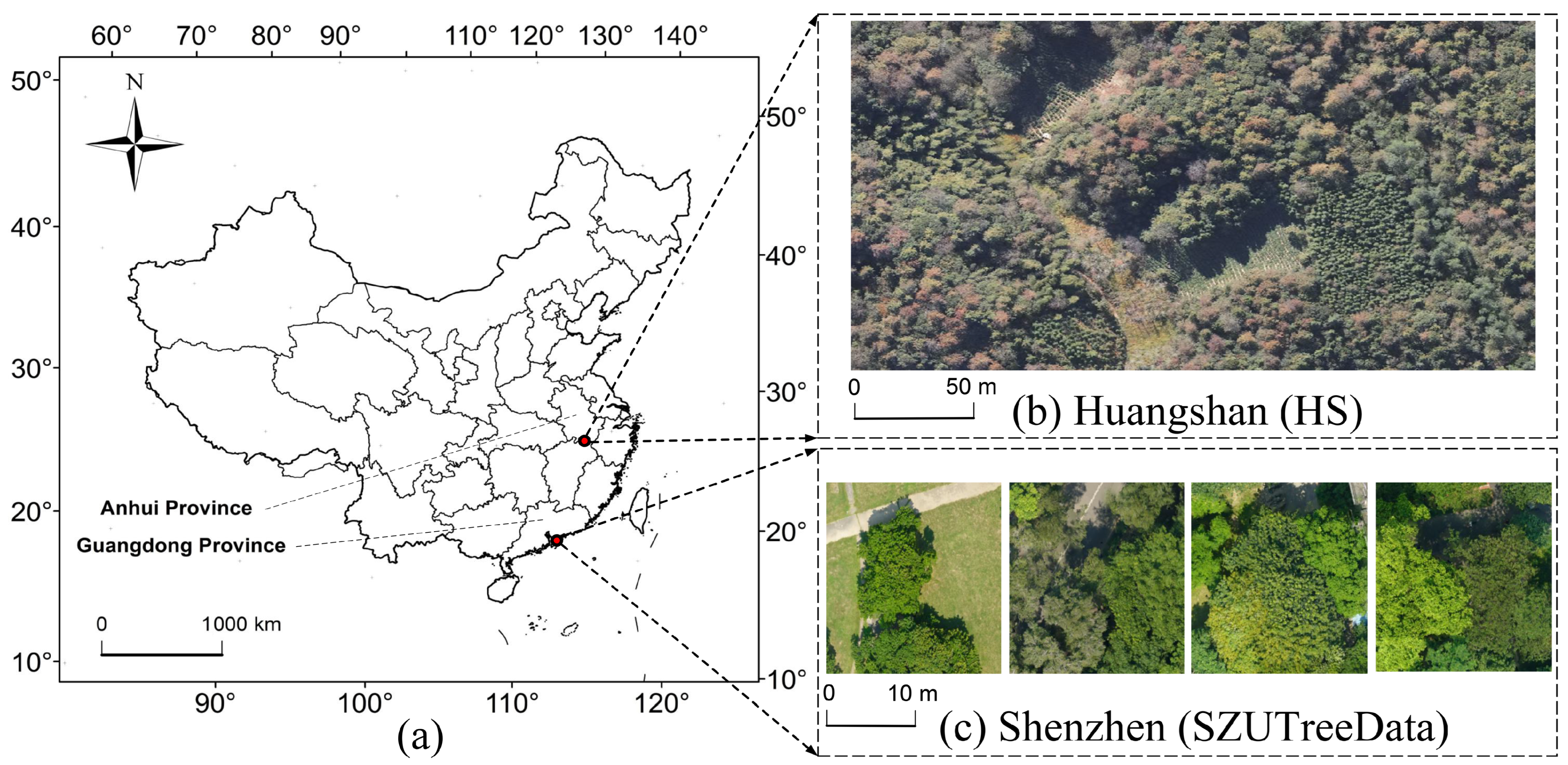
The study area is located in Qimen County, Huangshan City, Anhui Province, China, with a geographic extent of approximately 29. 60^∘–30. 14^∘N and 117. 20^∘–117. 95^∘E, as shown in Figure 1a. A total of 69 sample plots were surveyed in this region, covering the main tree species categories involved in this study, such as Pinus elliottii, Cunninghamia lanceolata, and Quercus spp. The region has a subtropical monsoon climate, with an average annual temperature ranging from 11 ^∘C to 22 ^∘C, evenly distributed precipitation, and extreme temperatures of 38 ^∘C (maximum) and −8 ^∘C (minimum). The terrain is primarily low and medium mountains and hills with significant undulating slopes. Forest coverage is approximately 88% of the area, with a ratio of planted to natural forest of approximately 7:3. Forest types are diverse, mainly including coniferous, broadleaf, mixed, and bamboo forests. The tree species include Pinus elliottii, Cunninghamia lanceolata, Quercus spp. and Liquidambar formosana, and are distributed in a banded or patchy pattern in some areas, as shown in Figure 1b. The dominant tree species and their proportional distributions across plots and image tiles are listed in

Table 1. HS crown-level tree species dataset: dominant classes and distribution.

Tree Species	Abbreviation	Crowns ($\times {10}^3$)	Plots	Tile Freq. (%)	Pixel Share (%)
Pinus elliottii	Pi.s	3.3	7	56.3	11.0
Cunninghamia lanceolata	Cu.l	3.8	10	63.7	12.6
Quercus spp.	Qu.s	3.0	8	49.1	10.2
Liquidambar formosana	Li.f	2.6	7	52.9	9.0
Eucalyptus globulus	Eu.g	2.8	6	51.1	9.4
Phyllostachys edulis	Ph.e	3.1	5	36.2	10.8
Camellia sinensis (tea)	Ca.s	1.6	9	26.7	5.4
Paulownia spp.	Pa.a	2.0	5	33.4	6.6
Other hard broadleaf (e.g., Schima, Cinnamomum, Sassafras, Catalpa, Melia, Populus)	Ot.b	2.6	14	71.8	8.7
Dead tree	De.t	0.7	5	12.6	1.8
Totals (foreground)		25.5	—	—	85.5

. Aerial data were acquired using a DJI Matrice 300 RTK drone equipped with a Zenmuse P1 full-frame RGB camera with approximately 45 megapixels and a focal length of 35 mm. The flight altitude was approximately 490 m, corresponding to a ground resolution of approximately 6.2 cm/pixel. The data were acquired in mid-October 2022 under clear, windless conditions, with forward and side overlaps of 80% and 70%, respectively. After aerial triangulation, orthorectification, and mosaicking, the images were converted into high-resolution orthophotos covering approximately 40 km². Furthermore, to assess cross-regional generalization, the publicly available SZUTreeData [12], collected from subtropical urban green spaces in Shenzhen, southern China, was used, as shown in Figure 1c. Example species include Terminalia arjuna, Ficus altissima, Delonix regia, Litchi chinensis, Mangifera indica, and Ficus virens. To maintain label consistency, the semantic annotations were normalized and geometrically corrected, including closed polygons, self-intersection removal, and boundary smoothing. Only the RGB and semantic mask components were retained for training and validation.

2.2. Dataset Construction and Preprocessing

The dataset uses crown-level polygon annotations and is studied under a species-level semantic segmentation setting. UAV RGB imagery was manually annotated based on field survey records and forest resource inventory data. Interpreters delineated crown polygons on orthophotos and assigned a species label to each annotation. Adjacent crowns were annotated as separate individuals only when a discernible inter-crown boundary was visible in the orthophoto; otherwise, they were retained as a continuous crown region. For blurred or partially occluded crowns, boundaries were delineated with reference to the visible crown contour and local canopy continuity. Understory vegetation was excluded from annotation. Dead trees were labeled as an independent class, whereas infrequent broadleaf taxa with limited crown-level samples were assigned to the “Other hard broadleaf” class. All annotations were reviewed and cross-validated by two additional interpreters to ensure spatial accuracy and class consistency. The original mosaic was cropped into fixed-size samples using ArcGIS 10.6. After removing areas with excessive non-forested land or missing crown, samples were grouped by plot to avoid spatial overlap. Geometric augmentation employed random rotation, flipping, and scale perturbation, while color perturbation was applied only to spectral channels. RGB inputs were normalized to zero mean and unit variance per channel. The depth prior was generated offline from the corresponding RGB imagery using publicly available pretrained monocular depth models. In the main experiments, Depth Anything V2 was used as the default depth source. No domain-specific fine-tuning was performed. For all compared depth estimators, the predicted depth maps were resampled to the RGB grid and processed with the same alignment and percentile-normalization procedure before being used as static geometric inputs.

2.3. Datasets and Evaluation Protocols

Regarding the datasets, HS is a self-constructed UAV RGB dataset annotated at the crown level and used in this study under a species-level semantic segmentation setting. Its collection, annotation, and class composition have been summarized above. SZUTreeData is a public dataset merged from two phases. The RGB orthophotos for R1 are 6170 × 4810 pixels in size, and those for R2 are 8080 × 4888 pixels in size. The HSI and LiDAR images included in the public dataset are not used in this article. The two phases together cover over 500 individual tree annotations. To facilitate cross-phase integration and comparison, we standardized category naming and performed label alignment. Furthermore, TreeAI is used here in the form of a publicly released UAV semantic segmentation dataset from Zenodo. It consists of two datasets: 1776 fully annotated images with a high annotation density, and 2051 partially annotated images with a lower annotation density. Due to the large number of original categories and the presence of homonymous or closely related classes across regions, we mapped them into a label space consisting of 20 target classes. Twelve of these are key tree species, such as Betula papyrifera, Tsuga canadensis, and Pinus sylvestris, and eight are genus-level groups, such as Acer spp., Quercus spp., and Pinus spp. For TreeAI, mIoU, AF, and OA are computed over a unified 20-class label space, where genus groups exclude pixels of the listed key species to avoid double counting. HS represents dense subtropical forest stands with crown-level species annotations, SZUTreeData represents urban tree scenes with more heterogeneous background interference, and TreeAI covers richer taxonomy under both fully labeled and partially labeled protocols, resulting in clear differences in region, taxonomy granularity, crown density, and annotation setting across the three datasets. It is worth noting that, to standardize the experimental setup, supervision is based solely on UAV RGB imagery and the corresponding semantic annotations. Since monocular depth is inferred offline from the same RGB data, it is used only as a frozen geometric prior and does not participate in gradient updates.

At the pixel level, the target task is evaluated as a semantic segmentation problem. Therefore, we quantitatively evaluate the model using common metrics in the segmentation field: mean Intersection over Union (mIoU), Macro-averaged F1 score (AF), and overall accuracy (OA). For HS and SZUTreeData, mIoU and AF are computed over foreground classes, while OA follows the standard pixel-wise definition, with unannotated pixels ignored. For fair comparison, all methods share the same tiling, augmentation, and sliding-window inference protocol under the same RGB-acquisition and semantic-supervision setting. First, we slice large orthophotos into 512 × 512 tiles. During training, we apply random scale crops, horizontal/vertical flips, and mild color perturbations, and apply identical geometric transforms to RGB and the cached depth prior to maintain pixel-level alignment. Second, during inference, we use overlapping sliding windows and cosine-weighted fusion to mitigate patchwork artifacts. Depth is used only by MCrown (and RGB–D baselines in ablations) as a frozen prior inferred from the same RGB. Monocular depth is inferred offline from RGB using Depth Anything V2 and cached before segmentation training and inference. The depth estimator is kept frozen, and no domain-specific fine-tuning is applied. The reported inference speed and memory consumption refer only to the segmentation model and do not include the cost of offline depth generation. Finally, we use the AdamW optimizer with a cosine learning rate schedule. For each fold, the checkpoint with the best validation performance was selected, and the reported HS and SZUTreeData results are averages over the four spatially disjoint test folds. All experiments were performed on a single-GPU desktop. The environment and hyperparameters are shown in

Table 2. Experimental environment and parameter settings.

Item	Setting
Platform	PyTorch 2.5.1
GPU	NVIDIA RTX 3070 Ti (8 GB)
CUDA version	12.1
Optimizer	AdamW
Learning rate	6 × 10−5
Weight decay	0.01
Iterations	80,000
Batch size	4
Input size	512 × 512

.

For data partitioning, HS and SZUTreeData are divided into four mutually exclusive folds with no spatial overlap. Each iteration involves training on three folds and testing on the remaining one, and we average the results from the four test runs to obtain a robust performance estimate. This strategy maximizes data utilization for reliable evaluation. For the TreeAI dataset, we adhered to its official partitioning scheme, conducting independent evaluations under both fully labeled and partially labeled settings without cross-subsets for training and testing.

2.4. Overview of MCrown

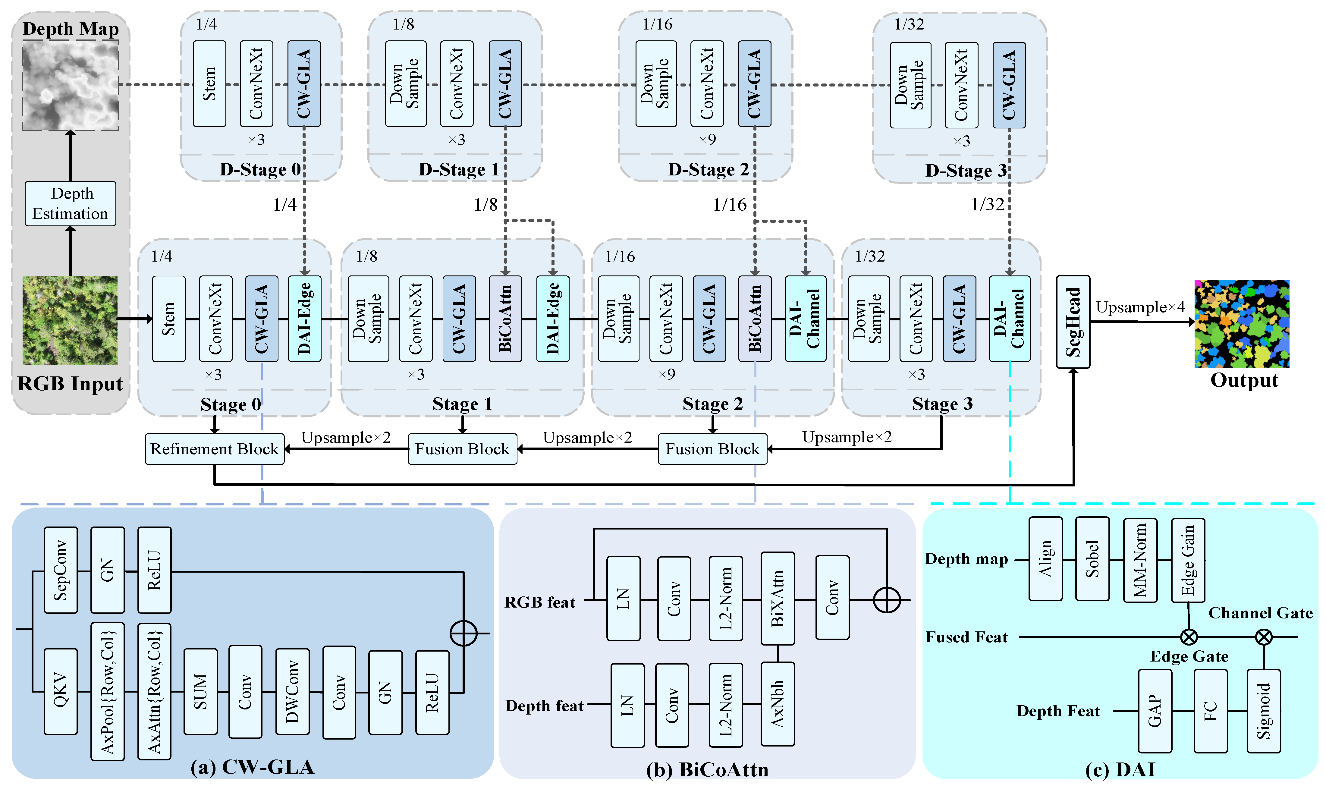
In this work, we propose MCrown, a crown-level tree species semantic segmentation framework built on appearance–geometry collaboration. The method uses single-temporal UAV RGB imagery as the only acquired and supervised modality, while treating a monocular depth map inferred offline from the same RGB image by Depth Anything V2 [37] as a frozen geometric prior rather than an independently acquired second modality. Rather than learning depth through an additional task-specific branch, the network uses this frozen prior to stabilize crown boundaries, reinforce structural continuity, and support morphological discrimination in complex forest scenes. The overall pipeline, illustrated in Figure 2, models crown semantics through CW-GLA–based context aggregation and depth-guided feature modulation. Below, we briefly outline the architecture and then describe each component in the subsequent subsections.

• Input preparation and dual-branch encoding. Given an input RGB image $I_{\mathrm{rgb}}\in {\mathbb{R}}^{H\times W\times 3}$, a depth map $D\in {\mathbb{R}}^{H\times W\times 1}$ is estimated using Depth Anything V2, resampled to the RGB grid, co-augmented with the same geometric transformations, and normalized on a per-patch basis using percentiles to reflect its relative scale. A symmetric dual-branch ConvNeXt encoder then extracts multi-scale RGB and depth feature maps across four stages. The depth estimator remains frozen and does not receive gradients, while each encoder stage incorporates a CW-GLA block to capture long-range contextual dependencies.
• Cross-modal interaction and depth-adaptive injection. Within the encoder, RGB and depth features are refined through two depth-guided mechanisms. A BiCoAttn module between Stages 1–2 performs sparse mutual attention in stripe-based neighborhoods, using depth-derived boundary cues to suppress illumination artifacts and spatially align appearance and geometry in textured regions. In parallel, the DAI mechanism injects geometric priors in a stage-aware manner: DAI-Edge in shallow stages (Stages 0–1) introduces Sobel-derived edge responses, while DAI-Channel in deeper stages (Stages 2–3) applies morphology-aware channel gating based on pooled depth features, enhancing crown contours and small-crown individuals.
• Adaptive multi-scale decoding and prediction. In the decoder, the depth-modulated RGB features from all four stages are projected to a unified channel dimension, progressively upsampled to the input resolution, and fused by the ConvexMix module, which predicts soft per-scale weights and produces a fused representation $F_{\mathrm{fuse}}\in {\mathbb{R}}^{H\times W\times C}$. A lightweight SegHead then maps F_fuse to per-pixel logits $P\in {\mathbb{R}}^{H\times W\times K}$ for K tree species classes.

Together, these components form an efficient architecture that jointly models appearance and geometry, enabling accurate crown-level tree species semantic segmentation from single-temporal UAV RGB imagery with a frozen monocular depth prior.

2.5. Context Aggregation Attention Module

High-resolution UAV orthophotos for ITSC require precise crown boundaries and long-range contextual cues. Pure convolutions remain local unless using very large kernels, while vanilla global self-attention incurs quadratic complexity in the number of tokens, so we adopted CW-GLA, which combines a lightweight convolutional path with stripe-based attention to balance accuracy and efficiency. As illustrated in Figure 2a, the output of the previous stage first undergoes layer normalization (LN) and is then processed in parallel by the local and global paths. To avoid redundant computation on high-resolution features, the local path uses depthwise separable convolution (DWConv) [38] with residual connections. DWConv’s channel-wise computation reduces the number of parameters and FLOPs, and the residual structure helps preserve details and maintain gradient stability. In contrast, the global path borrows the idea of axial attention, but does not perform global modeling across the entire row or column. Instead, it performs scaled dot–product attention within stripe windows of width w, where w is measured in tokens per stripe. We set the number of attention heads h and the stripe width w to 8 and adopted stripe-wise windows [39]. This design effectively avoids quadratic-time complexity while maintaining long-range dependencies. Assuming the input is $X\in {\mathbb{R}}^{N_l\times C_l}$, where N_l = H_lW_l and d is the per-head key dimension, the attention within a stripe t ∈ {row, col} is calculated as

$$O_t=softmax\left({\displaystyle \frac{Q_t{K}_t^{\top }}{\sqrt{d}}}+{\mathcal{M}}_t\right)V_t,$$

(1)

where Q_t, K_t, and V_t are obtained by linearly projecting X, then partitioned into stripes. ${\mathcal{M}}_t$ is a fixed additive attention mask, taking 0 on valid positions and −∞ otherwise, so attention is restricted to the stripe window. The row-wise and column-wise aggregation results are denoted as O_r and O_c, respectively. Since each token interacts only with w neighbors, this design reduces the quadratic complexity of standard self-attention, $\mathcal{O}\left(h{N}_l^2\right)$, to linear complexity, $\mathcal{O}\left(h{N}_{l}w\right)$, where h is the number of attention heads and N_l denotes the number of tokens. The final output is expressed as

$$X^{\prime }={\tilde{X}}_{\mathrm{loc}}+(O_r+O_c)W^O,$$

(2)

where ${\tilde{X}}_{\mathrm{loc}}$ is the local path output, and W^O is a 1 × 1 projection. Compared to traditional global attention, this striped modeling preserves long-range dependencies while avoiding quadratic overhead. Compared to purely local convolution, stripe attention can span the arrangements between tree crowns, strengthening the modeling of linear structures and forest belt patterns. In practice, it preserves edge sharpness on small-crown objects while maintaining global consistency in large crown areas, achieving a balance between efficiency and accuracy.

2.6. Bidirectional Information Alignment

In high-resolution UAV imagery, RGB features provide rich texture and spectral details, while depth features supply complementary geometric and morphological cues of the tree crown. Simple fusion by concatenation or element-wise addition tends to ignore modality-specific statistics and can yield redundant or even conflicting responses, especially when the auxiliary depth is noisy [40]. Existing attention-based fusion methods alleviate this to some extent but often introduce high computational overhead and still lack explicit constraints on geometric boundaries [33]. To address these issues, we designed a layer-wise bidirectional interaction module in the intermediate encoder stage, whose core structure is shown in Figure 2b.

We denote the stripe-constrained cross-attention sublayer in BiCoAttn as BiXAttn, and AxNbh constructs the axial stripe neighborhoods ${\mathcal{N}}_t\left(i\right)$ and the corresponding binary mask M(i, j). First, the RGB and depth features $F_R^l,F_D^l\in {\mathbb{R}}^{N_l\times C_l}$ are projected using LN and a 1 × 1 convolution, where l indexes the encoder stage, $N_l=H_l{W}_l$ is the number of tokens, and C_l is the channel dimension. LN reduces distribution differences between modalities and is more suitable than BN for Transformer-style token sequences [41], while the 1 × 1 convolution aligns and compresses channels to reduce subsequent computation. The projected features are then row-wise ℓ ₂-normalized to obtain ${\tilde{F}}_R^l,{\tilde{F}}_D^l$, so that similarity depends only on feature direction rather than magnitude, effectively implementing a cosine similarity measure within the stripe-constrained attention. To highlight geometric boundaries, we compute a boundary score from the Sobel gradient magnitude of the depth map, normalize it by min–max scaling, and denote it by b. Instead of raw depth values, b is added as a bias before softmax to enhance boundary tokens and suppress spurious edges from lighting or shadows, following the idea of prior enhancement in boundary-guided segmentation.

In the interaction phase, we introduce stripe-constrained interactive attention instead of standard global attention. Similar to Axial Attention, AxNbh constructs the neighborhood ${\mathcal{N}}_t\left(i\right)$ (t ∈ {row, col}) along the row or column direction and provides the binary mask M(i, j); the window width is further restricted to w with stripe-constrained neighborhoods to avoid redundant interactions across the entire row and column. The interaction weight is defined by the similarity score $s_{D\to R}^l(i,j)$ between the i-th RGB token and the j-th depth token, which is later normalized by a softmax operation:

$$\begin{array}{cc}\hfill s_{D\to R}^l(i,j)& ={\tilde{F}}_R^l{\left(i\right)}^{\top }{\tilde{F}}_D^l\left(j\right)+b_j,\hfill \\ \hfill P_{D\to R}^l(i,j)& ={\displaystyle \frac{M(i,j)exp\left(s_{D\to R}^l(i,j)\right)}{{\displaystyle \sum _{j^{\prime }\in {\mathcal{N}}_t\left(i\right)}}M(i,j^{\prime })exp\left(s_{D\to R}^l(i,j^{\prime })\right)}}.\hfill \end{array}$$

(3)

where M(i, j) ∈ {0, 1} is a binary neighborhood mask (multiplicative), distinct from the additive mask ${\mathcal{M}}_t$ in Equation (1); $j^{\prime }$ ranges over this set, b_j is the boundary prior, and $P_{D\to R}^l(i,j)$ denotes the normalized attention weight from the j-th depth token to the i-th RGB token. With this mask, each token interacts with at most w neighbors per stripe, which localizes computation and reduces complexity. Cross-modal information is exchanged through a gated residual update:

$${\widehat{F}}_R^l=F_R^l+\eta \odot \left(P_{D\to R}^l{F}_D^l\right)W^R,$$

(4)

where W^R is a 1 × 1 projection. A symmetric update is also applied for ${\widehat{F}}_D^l$, where depth tokens receive complementary information from RGB. Here, η is a channel-wise gate with values between 0 and 1, computed from the global averages of $F_R^l$ and $F_D^l$ through a linear projection followed by a sigmoid, and broadcast across the token dimension. η further adjusts the strength of cross-modal transfer in the channel dimension, avoiding over-coupling when the quality of one modality is insufficient.

2.7. Geometry-Guided Feature Enhancement

Depth information in high-resolution UAV imagery can effectively supplement geometric information that is difficult to obtain in RGB modalities. Specifically, it contains clear local boundary cues and provides a statistical prior for overall crown morphology. Existing methods often use cross-modal alignment mechanisms to integrate multi-source features [32]. However, such schemes often ignore the differentiated requirements for geometric information at different stages. For example, shallow layers require fine-grained boundary constraints, while deep layers rely more on global morphological priors. Based on this, we proposed the Depth-Adaptive Injection (DAI) mechanism, the structure of which is shown in Figure 2c. The core concept of DAI is staged modulation. In the early stages, the model requires stronger boundary guidance to compensate for the ambiguity of RGB features between adjacent canopies. We constructed an edge gain term based on the gradient magnitude of the stage-aligned depth map D^l, where D^l is D resized to H_l × W_l:

$$E^l=\text{MM-Norm}\left(\mathrm{Sobel}\left(D^l\right)\right),E^l\in {[0,1]}^{H_l\times W_l},$$

(5)

where MM - Norm denotes min–max normalization to [0, 1]. This term enhances the discrimination of crown edges on a pixel-by-pixel basis. In later stages, feature resolution decreases, making it more suitable for extracting overall morphology. We then used the depth branch features $F_D^l$ to obtain channel weights through global average pooling (GAP) and a linear projection:

$${\mathbf{c}}^l=\sigma \left(\mathrm{GAP}\left(F_D^l\right)W_c^l\right),{\mathbf{c}}^l\in {[0,1]}^{C_l},$$

(6)

where $W_c^l$ is a learnable projection matrix and σ(·) denotes the sigmoid activation. This vector is reweighted along the channel dimension to amplify structural features consistent with the overall outline of the tree crown and suppress redundant textures. In other words, the fused features at stage l can be uniformly expressed as:

$$F^l=\left\{\begin{array}{cc}{F}_{\mathrm{cm}}^l\odot (1+E^l),\hfill & l\in \{0,1\},\hfill \\ F_{\mathrm{cm}}^l\odot (1+{\mathbf{c}}^l),\hfill & l\in \{2,3\},\hfill \end{array}\right.$$

(7)

where $F_{\mathrm{cm}}^l$ is the intermediate RGB feature (${\widehat{F}}_R^l$) after cross-modal fusion, and ⊙ represents element-wise multiplication. Unlike common general-purpose attention mechanisms, DAI explicitly incorporates deep geometric evidence into semantic feature learning through a progressive modulation strategy from “edge-first to morphology-first.” Its computation relies only on a Sobel filter and channel-wise linear gating, with negligible additional parameters introduced.

2.8. Decoder Fusion and Loss Function

During the decoding phase, the fused features from the four layers are first upsampled to the input resolution and unified to the same channel dimension via a 1 × 1 convolution. Subsequently, a lightweight gating branch predicts weights for each pixel at different scales and normalizes them across the scale dimension using a softmax function to achieve dynamic multi-scale fusion. Unlike fixed weighting approaches, this strategy adaptively adjusts the contribution of each scale based on the feature distribution of the input region, reducing reliance on a single resolution. The resulting fused representation is fed into the classification head to generate class logits. A composite loss function is used during network training:

$$\mathcal{L}={\mathcal{L}}_{\mathrm{CE}}+{\lambda }_{\mathrm{dice}}{\mathcal{L}}_{\mathrm{Dice}}+{\lambda }_{\mathrm{edge}}{\mathcal{L}}_{\mathrm{BCE}}^{\mathrm{edge}},$$

(8)

where ${\mathcal{L}}_{\mathrm{CE}}$ is the class-weighted cross-entropy, which alleviates class imbalance through a balancing strategy based on the effective number of samples [42]; ${\mathcal{L}}_{\mathrm{Dice}}$ is used to improve the segmentation accuracy of small-crown objects; ${\mathcal{L}}_{\mathrm{BCE}}^{\mathrm{edge}}$ supervises a boundary target derived from the ground-truth masks to refine crown contours. Following boundary-aware segmentation practice, we determined the loss weights λ_dice and λ_edge by a one-time grid search on the held-out validation split and kept them fixed across all experiments [31]. The RGB and depth branches share the same geometric augmentation to maintain spatial alignment. The monocular depth estimation module remains frozen during training and only participates in the geometric prior constraint.

3. Results

This section presents the comparative and ablation results of MCrown on HS, SZUTreeData, and TreeAI.

3.1. HS Results

To evaluate the performance of the proposed MCrown, we conducted comparative evaluations with representative convolutional networks, Transformer, and state-space models. These include the CNN-based DeepLabv3+ [43], HRNetV2+OCR [44], and UPerNet [45] based on ConvNeXt-L; the Transformer-based SETR-ML/L [46], Segmenter [47], Swin-UNet [25], SegFormer-B5 [24], TransUNet [48], MaskFormer [49], Mask2Former [23], SegViT [50], and UPerNet based on Swin-L; and the modern hybrid architecture models SegNeXt [51], K-Net [52], and UNetFormer [53]; as well as VMamba-UNet [27] based on a state-space hybrid architecture.

Table 3. Results on the HS crown-level tree species dataset (per-class IoU, %). Best values are bold and underlined.

Method	Pi.s	Cu.l	Qu.s	Li.f	Eu.g	Ph.e	Ca.s	Pa.a	Ot.b	De.t	mIoU	AF	OA
DeepLabv3+	72.1	71.8	71.6	74.3	76.2	70.7	50.2	68.2	65.3	50.0	67.0	79.9	80.5
HRNetV2+OCR	73.3	73.4	74.3	74.0	79.5	72.4	51.6	70.4	65.3	49.8	68.4	80.8	82.5
SETR-MLA	72.5	76.0	73.8	74.7	76.1	71.4	50.2	75.4	70.3	50.1	69.1	81.2	83.5
Segmenter	73.2	75.3	75.5	74.2	74.9	73.2	51.3	74.9	72.3	51.2	69.6	81.7	84.2
K-Net	75.3	74.9	72.7	74.5	76.2	74.9	51.8	77.0	72.4	52.1	70.2	82.1	84.3
UNetFormer	74.9	74.8	73.5	72.7	77.4	75.7	52.1	76.3	73.2	54.3	70.5	82.4	84.5
UPerNet (ConvNeXt-L)	77.0	75.8	74.1	73.4	77.6	76.4	51.0	75.6	73.3	53.5	70.8	82.5	84.5
Swin-UNet	77.0	74.7	76.4	74.3	76.4	75.7	53.5	76.6	72.9	53.2	71.1	82.7	84.8
SegNeXt	76.2	75.6	76.2	75.6	79.3	76.7	51.3	76.4	73.3	56.1	71.7	83.1	85.0
MaskFormer	76.8	76.3	76.0	76.0	78.2	77.5	51.8	78.2	74.6	57.2	72.3	83.5	86.3
UPerNet (Swin-L)	77.2	77.8	75.4	74.6	78.4	77.3	51.9	79.5	74.6	56.9	72.4	83.6	85.6
TransUNet	76.1	76.9	76.0	74.9	79.9	78.8	52.7	78.3	74.3	57.6	72.6	83.8	85.0
SegFormer-B5	76.8	76.6	75.6	76.8	79.7	77.9	53.4	78.5	75.0	56.6	72.7	83.8	85.2
SegViT	77.7	76.1	75.9	76.4	81.5	80.1	53.3	78.6	74.7	56.7	73.1	84.1	86.8
Mask2Former	77.3	77.0	76.1	76.9	81.7	78.4	53.3	79.4	75.3	57.9	73.3	84.3	86.8
VMamba-UNet	77.8	76.4	76.6	76.0	82.2	79.5	53.6	80.0	74.2	58.8	73.5	84.4	86.9
MCrown (ours)	78.6	77.4	75.8	76.6	82.9	80.1	54.8	80.5	74.6	59.2	74.1	84.8	87.3

Class names: Pi.s—Pinus elliottii; Cu.l—Cunninghamia lanceolata; Qu.s—Quercus spp.; Li.f—Liquidambar formosana; Eu.g—Eucalyptus globulus; Ph.e—Phyllostachys edulis; Ca.s—Camellia sinensis (tea); Pa.a—Paulownia spp.; Ot.b—other hard broadleaf; De.t—dead tree.

shows the results of the compared methods on the HS dataset. To improve readability, we focus the following discussion on the main overall metrics and on categories that more clearly reflect boundary ambiguity, local fragmentation, or small-crown difficulty. For reference, the abbreviated class names are expanded at first appearance in the main text: Pi.s (Pinus elliottii), Cu.l (Cunninghamia lanceolata), Qu.s (Quercus spp.), Li.f (Liquidambar formosana), Eu.g (Eucalyptus globulus), Ph.e (Phyllostachys edulis), Ca.s (Camellia sinensis), Pa.a (Paulownia spp.), Ot.b (other hard broadleaf), and De.t (dead tree). The category-wise results suggest that the proposed design is particularly beneficial for crowns that are small, locally fragmented, or easily confused with surrounding vegetation. In such cases, the contribution of the depth prior is reflected more directly in clearer boundary separation and more stable preservation of local crown shape, particularly when adjacent crowns exhibit similar textures or colors and RGB appearance alone is insufficient for reliable separation. Therefore, the advantage of MCrown is reflected not only in mIoU, but also in more stable boundary delineation and crown-structure preservation under complex canopy conditions.

For the three standard metrics, mIoU, AF, and OA, the proposed model achieved 74.1%, 84.8%, and 87.3%, respectively. Among the compared methods, MCrown achieved the strongest overall performance under the current evaluation setting. Compared with VMamba-UNet, MCrown improved mIoU, AF, and OA by 0.6%, 0.4%, and 0.4%, respectively. Although the overall mIoU gain is modest, the advantage is more evident in categories affected by boundary ambiguity, local fragmentation, and small crowns. Specifically, the mIoU for the “Ca.s” class improved by 1.2% compared to VMamba-UNet. We attribute this improvement to the boundary cues introduced by the deep adaptive injection mechanism in the early layers, which more accurately delineate the low-height tea hedgerows and their fine margins. For the “Pi.s” class, the improved result may be related to the ability of cross-window global–local attention to better capture fine-grained coniferous structures and reduce over-fusion between adjacent crowns. Overall, MCrown achieved strong performance on most classes, suggesting improved feature discrimination for pixel-wise species segmentation. Notably, MCrown did not show a clear advantage on “Ot.b” in terms of IoU, while it still maintained leading segmentation performance for most classes overall. Furthermore, all models generally performed poorly for the “Ca.s” class. We speculate that the main reason for this is that the crown height of economic forests, such as tea plantations, is low and regularly distributed, resulting in insufficient crown edge clarity at the crown level. Similarly, “De.t” is a difficult category to identify because dead trees typically have exposed canopies and sparse textures, and their crown edges are affected by light and shadow. These characteristics are similar to those of some deciduous trees in drone remote sensing imagery, limiting overall classification accuracy.

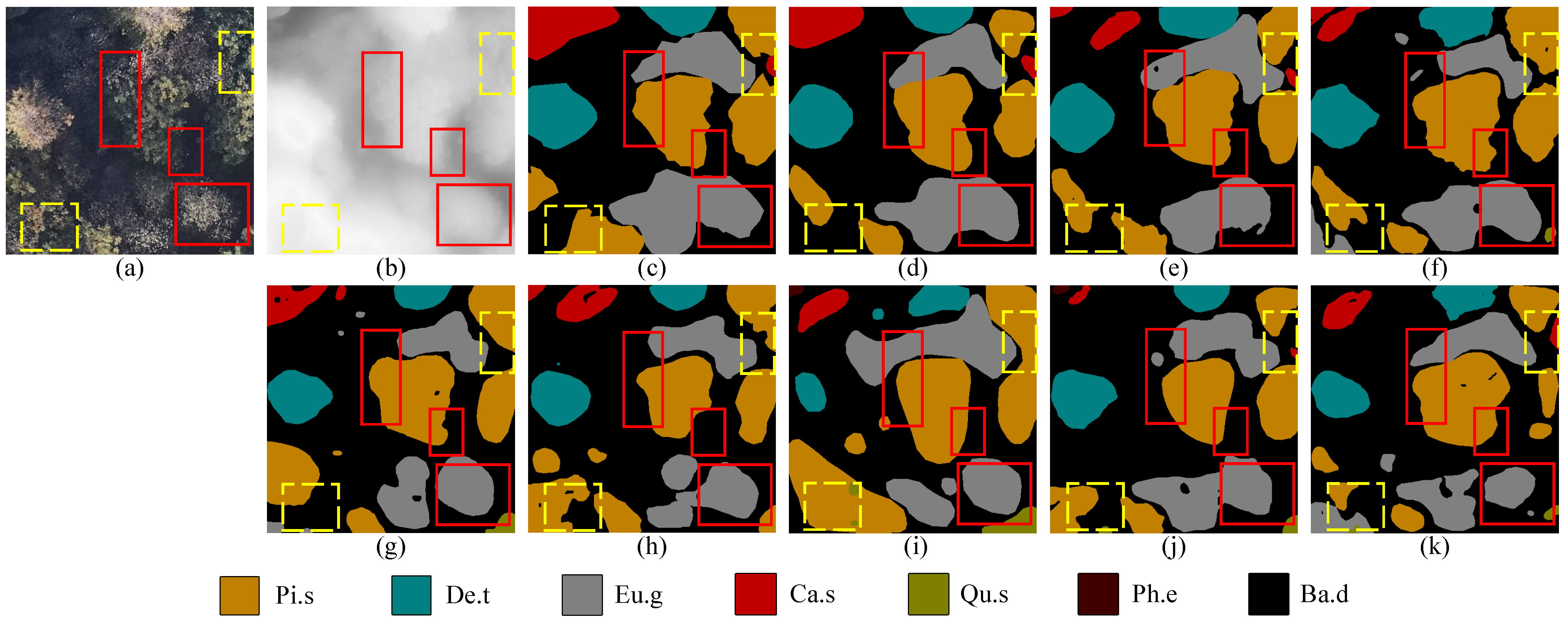
To visually compare the segmentation performance of different methods at the crown level, we visualized the prediction results for the same scene, as shown in Figure 3. MCrown produced clearer and more continuous crown segmentation results overall. For example, within the representative regions highlighted by the red boxes, MCrown produced clearer boundaries for categories such as “Eu.g” and “Pi.s”, with more continuous crown structures and less fragmentation than the comparison methods. In contrast, the other methods exhibited fragmented artifacts in the same area, with some crown edges showing breakage and backfilling. Notably, the depth map provided stable geometric constraints in this scenario, enabling the model to better align crown edges and suppress artifacts caused by shadows or background noise. MCrown’s predictions maintained more continuous crown regions and reduced scattered false positives. In addition to the representative regions highlighted by the red boxes, the yellow dashed boxes indicate challenging areas with residual errors. In these regions, shadowed Pinus elliottii crowns can still be segmented incompletely, whereas Camellia sinensis near image margins or canopy gaps can exhibit local confusion with neighboring classes.

3.2. SZUTreeData Results

To verify the generalization ability of the proposed model in urban scenes, we conducted experiments on the public dataset SZUTreeData. The prediction results are shown in

Table 4. SZUTreeData test results (per-class IoU, %). Best values are bold and underlined.

Method	Te.a	Ki.a	Ro.r	Fi.a	De.r	Lt.c	Ma.i	Ar.c	Lv.c	Dr.d	Ac.c	Fi.m	Fi.e	Ba.b	Me.c	Fi.v	Ca.e	Sw.m	mIoU	AF	OA
DeepLabv3+	70.5	57.5	79.2	68.8	78.9	77.2	60.3	74.5	79.6	69.3	60.5	72.3	80.4	74.9	73.9	80.9	57.9	80.5	72.1	83.5	86.9
SETR-MLA	72.5	58.6	80.5	70.5	80.4	77.5	61.2	76.1	80.7	70.5	61.3	72.8	81.3	76.3	75.4	82.8	58.7	81.5	73.3	84.3	86.3
HRNetV2+OCR	72.9	59.0	80.9	70.8	80.0	78.7	61.3	76.9	81.8	71.2	61.8	72.2	82.1	76.6	75.4	82.7	59.1	81.9	73.6	84.6	87.0
Segmenter	73.6	60.2	82.2	71.4	80.6	79.1	61.7	78.6	82.8	71.5	63.3	73.2	82.8	77.1	76.0	83.4	59.5	82.2	74.4	85.1	86.4
K-Net	74.2	61.4	83.9	71.7	81.0	79.7	61.1	79.8	82.9	72.0	63.0	73.2	82.8	76.8	75.9	83.2	59.8	82.9	74.7	85.3	86.0
UNetFormer	74.8	61.1	83.2	72.0	81.7	79.5	61.9	80.6	83.4	72.6	63.7	74.2	83.7	77.6	76.3	83.6	60.4	83.6	75.2	85.6	87.1
SegNeXt	77.2	60.4	84.2	72.6	82.5	80.2	61.5	81.2	83.4	72.3	63.3	74.2	84.1	77.7	76.8	83.3	60.7	83.9	75.5	85.8	87.8
Swin-UNet	75.1	61.0	83.6	72.2	81.9	80.2	62.3	81.7	84.0	72.8	64.1	74.4	84.0	78.2	77.3	84.5	60.8	83.9	75.7	85.9	88.5
UPerNet (ConvNeXt-L)	75.0	61.5	83.7	72.1	81.9	80.0	63.3	83.5	82.9	72.2	64.3	74.2	83.5	77.9	77.0	84.2	61.0	83.6	75.7	86.0	88.0
UPerNet (Swin-L)	75.5	61.0	84.4	72.5	82.2	80.5	63.7	82.3	83.3	72.5	64.7	74.7	84.0	78.3	77.4	84.5	61.4	84.0	75.9	86.2	89.1
TransUNet	75.7	61.6	84.2	72.6	82.1	80.6	62.7	82.1	84.3	73.2	64.5	74.9	84.3	78.6	77.6	84.8	61.2	84.2	76.1	86.2	88.9
SegFormer-B5	76.1	61.9	85.0	73.2	82.7	81.0	61.9	81.8	84.1	73.0	64.1	75.1	84.8	78.7	77.8	85.1	60.8	85.4	76.3	86.3	89.3
MaskFormer	77.3	62.6	85.8	73.8	83.4	81.9	63.3	82.9	84.9	73.8	65.1	75.8	85.2	78.9	78.0	85.4	61.7	88.0	77.1	86.8	87.6
SegViT	78.1	63.4	87.0	74.4	83.6	82.2	63.7	83.6	85.3	74.1	65.5	79.3	85.6	79.3	78.4	85.8	62.1	87.3	77.7	87.2	88.6
Mask2Former	79.6	63.7	87.5	77.8	84.6	83.2	64.5	84.3	85.5	75.0	66.2	77.5	86.1	80.3	79.4	86.5	62.8	87.6	78.5	87.7	89.6
VMamba-UNet	80.3	64.3	88.9	76.8	84.1	83.0	65.9	84.8	85.8	75.6	71.0	78.0	86.8	80.7	79.8	87.1	63.3	87.1	79.1	88.1	90.2
MCrown (ours)	80.8	65.1	88.3	77.5	85.7	84.5	67.0	83.4	86.9	76.3	70.9	79.0	87.1	82.2	81.1	88.5	64.7	87.8	79.8	88.6	91.0

Abbreviations: Te.a = Terminalia arjuna, Ki.a = Kigelia africana, Ro.r = Roystonea regia, Fi.a = Ficus altissima Blume, De.r = Delonix regia, Lt.c = Litchi chinensis, Ma.i = Mangifera indica, Ar.c = Araucaria cunninghamii Aiton ex D.Don, Lv.c = Livistona chinensis, Dr.d = Dracontomelon duperreanum Pierre, Ac.c = Acacia confusa, Fi.m = Ficus microcarpa L.f., Fi.e = Ficus elastica, Ba.b = Bauhinia x blakeana, Me.c = Melaleuca cajuputi, Fi.v = Ficus virens, Ca.e = Casuarina equisetifolia, Sw.m = Swietenia macrophylla.

. For clarity, the discussion below emphasizes the main overall metrics and the categories showing more evident differences under complex urban backgrounds. On the standard evaluation metrics mIoU, AF, and OA, the proposed model achieved 79.8%, 88.6%, and 91.0% on the SZUTreeData test set, respectively. MCrown showed leading overall performance under the same protocol.

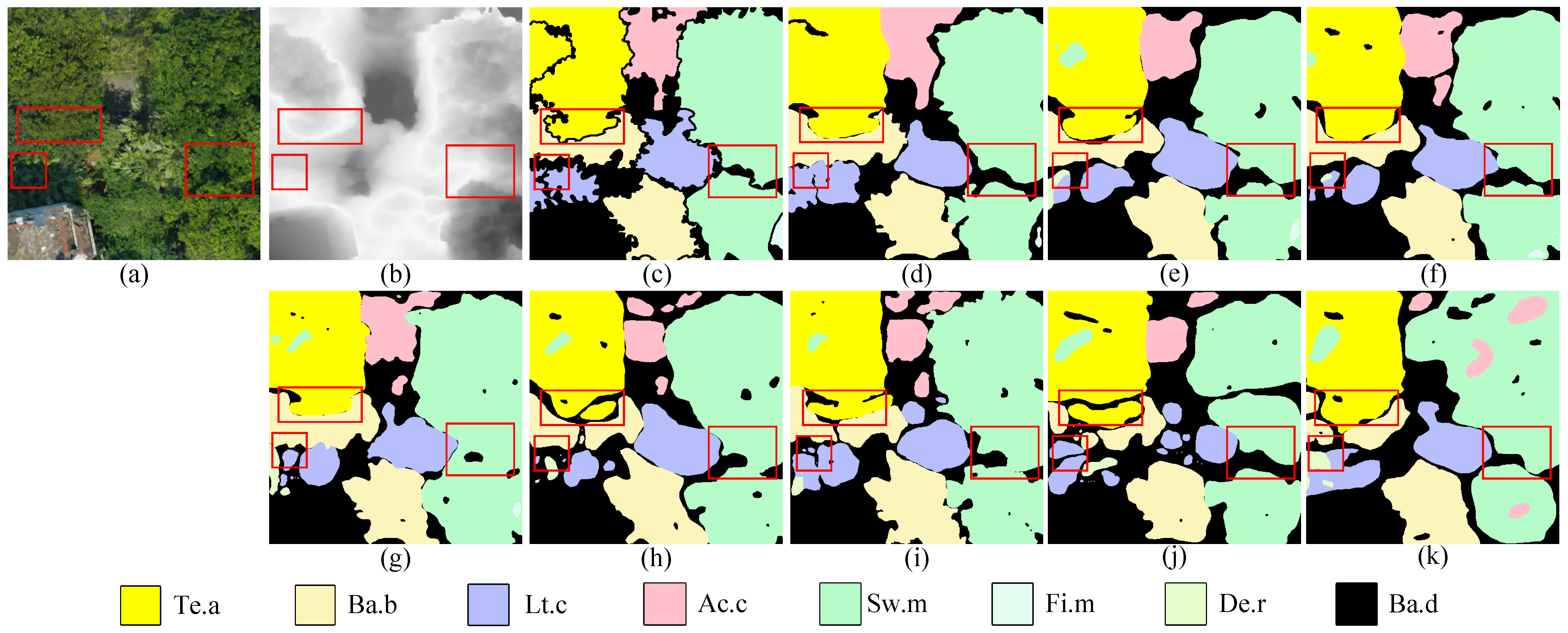
Furthermore, some classes in the SZUTreeData dataset occurred as scattered or strip-like crowns and were often adjacent to background areas such as roads and buildings. Blurred boundaries and lighting interference complicated accurate segmentation. For some categories, such as “Lt.c” and “Ba.b”, the IoU improved by 1.3% and 1.5% over the best-performing counterparts, Mask2Former and VMamba-UNet, respectively, indicating consistent gains for these categories. These categories often correspond to crowns that are narrow, irregular in shape, and adjacent to roads or buildings. MCrown maintained boundary integrity and reduced missegmentation in such scenarios, demonstrating the model’s adaptability to complex urban environments. We visualized the prediction results, as shown in Figure 4. In the red box region, some samples of “Lt.c” were misclassified as “De.r” by other methods, while MCrown produced more consistent “Lt.c” boundaries. Furthermore, existing methods often exhibited discontinuous or broken outlines in “Te.a” and “Sw.m”, while MCrown effectively maintained the integrity of tree crown boundaries. Some categories with irregular shapes and narrow crown widths, such as “Ac.c”, were more susceptible to background interference when adjacent to roads or buildings, which increased the difficulty of accurate identification and led to larger performance variations across models. To further show fold-to-fold variability on HS and SZUTreeData,

Table 5. Cross-fold variability of MCrown on HS and SZUTreeData for the main evaluation metrics (mean ± standard deviation, %).

Dataset	mIoU	AF	OA
HS	74.1 ± 0.77	84.8 ± 0.53	87.3 ± 0.40
SZUTreeData	79.8 ± 1.12	88.6 ± 0.91	91.0 ± 0.63

reports the mean ± standard deviation of MCrown across the four spatially disjoint folds. The reported standard deviations indicate that the model performance is relatively consistent across different spatial folds under the current protocol.

3.3. TreeAI Results

To further examine the proposed model’s adaptability to conditions with rich categories and complex annotation formats, we evaluated two subsets of the TreeAI dataset: the fully annotated subset, which covers the entire tree species catalog and provides dense pixel-level annotations; and the partially annotated subset, which records the main tree species categories in the form of sparse masks. Both subsets share the same classification system and indexing rules. The table reports per-class IoU for key species and genus groups for the fully labeled and partially labeled splits. It is important to note that unlabeled pixels in the partially annotated subset are not counted in model training or performance evaluation.

3.3.1. Full Supervision

Table 6. TreeAI_fL: IoU (%) for key species (left) and genus groups (right). Best values are bold and underlined.

	Key Species												Grouped Classes
Method	Be.p	Ts.c	Pn.s	Be.a	Ac.p	Ab.f	Qu.i	Be.g	Fa.s	Ab.a	Po.b	Ce.l	Ace	Que	Pic	Pin	Abi	Fag	Pop	Lar	mIoU	AF	OA
DeepLabv3+	78.0	72.3	54.7	69.8	58.6	47.9	53.5	76.1	66.8	56.7	68.4	45.9	69.8	58.4	66.2	54.3	56.1	66.0	68.2	64.0	62.6	76.6	90.8
HRNetV2+OCR	79.0	73.8	55.6	70.2	60.7	48.1	54.9	77.6	67.2	57.8	69.5	47.3	70.6	59.2	67.1	55.4	57.0	66.8	69.0	65.0	63.6	77.4	91.1
SegFormer-B5	80.1	75.4	56.9	71.5	61.8	50.2	55.7	78.9	68.1	58.6	70.7	49.8	72.8	61.0	67.9	56.1	58.2	68.0	70.1	66.0	64.9	78.4	91.4
K-Net	80.3	75.7	56.5	72.4	62.5	51.8	55.2	78.6	68.2	58.2	71.6	49.5	73.1	61.3	68.2	56.4	59.1	68.4	70.5	66.1	65.2	78.6	91.6
UPerNet (Swin-L)	80.8	76.9	57.8	72.8	62.9	51.4	56.6	79.2	69.4	59.1	71.9	50.7	73.7	62.0	69.0	57.1	59.0	69.0	70.8	66.8	65.8	79.1	91.8
UNetFormer	81.2	76.1	57.3	72.6	63.7	52.6	56.9	79.7	69.8	59.9	71.4	50.4	73.9	62.2	69.1	57.3	59.6	69.2	71.0	66.9	66.0	79.2	91.5
MaskFormer	82.5	78.8	59.3	74.7	65.5	54.1	58.6	81.5	71.7	60.4	72.5	53.6	75.4	63.7	70.6	58.9	61.2	71.2	72.2	68.8	67.8	80.5	91.9
Mask2Former	83.2	81.2	61.7	75.1	66.8	56.9	60.8	82.3	72.9	61.2	73.6	54.4	76.2	65.0	71.9	60.8	63.0	72.1	73.1	69.7	69.1	81.4	92.0
SegViT	83.6	80.6	61.5	75.9	67.2	56.7	60.5	83.6	72.4	62.2	74.8	55.1	77.0	65.2	75.1	61.0	63.4	72.5	74.0	70.2	69.6	81.8	92.1
VMamba-UNet	84.1	80.8	62.6	76.5	68.4	57.3	61.9	84.5	73.5	62.1	74.4	56.8	77.8	66.0	73.4	62.2	64.2	73.3	74.1	71.9	70.3	82.3	92.3
MCrown (ours)	85.3	81.1	63.5	77.1	69.2	59.6	63.0	85.0	74.0	62.6	75.1	54.8	78.9	66.8	74.2	63.1	65.5	75.4	75.0	71.4	71.0	82.8	92.6

Key species: Be.p = Betula papyrifera; Ts.c = Tsuga canadensis; Pn.s = Pinus sylvestris; Be.a = Betula alleghaniensis; Ac.p = Acer pensylvanicum; Ab.f = Abies firma; Qu.i = Quercus ilex; Be.g = Betula sp.; Fa.s = Fagus sylvatica; Ab.a = Abies alba; Po.b = Populus balsamifera; Ce.l = Cedrus libani. Genus groups (defined to exclude key-species pixels to avoid double counting). Ace = Acer spp. (e.g., A. saccharum, A. rubrum, A. platanoides, Acer sp.); Que = Quercus spp. (e.g., Q. robur, Q. petraea); Pic = Picea spp. (e.g., P. abies, P. rubens, P. mariana, Picea sp.); Pin = Pinus spp. (e.g., P. strobus, P. pinea, P. montezumae, P. koraiensis, P. nigra, P. elliottii, Pinus sp.); Abi = Abies spp. (e.g., A. holophylla, A. balsamea); Fag = Fagus spp. (e.g., F. grandifolia, F. crenata); Pop = Populus spp. (e.g., P. grandidentata); Lar = Larix spp. (e.g., L. laricina, L. decidua, L. 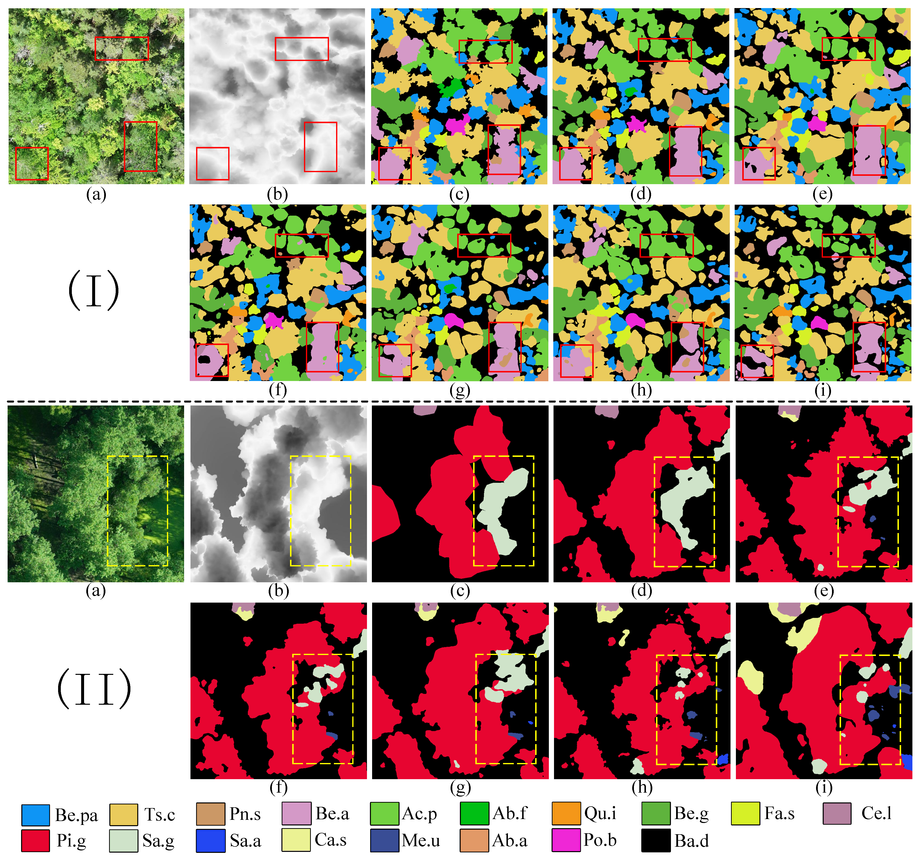gmelinii).

shows that MCrown achieved leading overall scores, with mIoU, AF, and OA of 71.0%, 82.8%, and 92.6%, respectively. Coniferous tree species such as “Pn.s” and “Ab.a” remained challenging, as they have slender crowns and thin branches, often intertwining with neighboring species. Despite this, the proposed model achieved higher IoU scores for these categories than the baselines. Visualization results are shown in Figure 5I. In the red box region, we observed that the crown of “Ac.p” was mistakenly segmented into continuous blocks in most comparison models, while its true distribution is discrete and prone to breakage or adhesion during segmentation. MCrown better separated adjacent crowns, reducing crown adhesion errors. Meanwhile, “Be.a” was prone to being confused with background regions by comparison methods due to its exposed trunk, often exhibiting highly reflective areas. The proposed model reduced such confusion, maintaining the stability of tree species identification. We also noted that the identification of “Pn.s” remained challenging. This species often grows in marginal locations, surrounded by neighboring species, and its texture features are highly similar to those of its surroundings, making it more difficult to distinguish.

3.3.2. Partial Labels

Table 7. TreeAI_pL: IoU (%) for key species (left) and genus groups (right). Best values are bold and underlined.

	Key Species												Grouped Classes
Method	Be.p	Pi.g	Sa.g	Sa.a	Ct.s	Me.u	Pi.a	Pn.s	La.d	Qu.r	Fa.s	Ab.a	Ace	Que	Pin	Abi	Pop	Lar	Til	Fra	mIoU	AF	OA
DeepLabv3+	72.5	65.2	52.4	58.1	61.5	49.3	73.0	54.0	56.8	59.0	59.6	55.7	68.0	60.0	55.5	56.6	67.9	63.8	60.5	58.7	60.4	75.1	91.6
HRNetV2+OCR	73.4	66.0	53.3	59.0	62.3	50.6	73.8	55.0	57.7	60.1	60.4	56.6	68.9	60.9	56.3	57.5	68.7	64.6	61.3	59.6	61.3	75.8	92.2
SegFormer-B5	74.9	67.2	54.7	60.2	63.7	52.0	75.1	56.2	58.9	61.6	61.8	57.9	70.1	62.2	57.2	58.7	69.8	65.6	62.4	60.7	62.5	76.8	92.6
K-Net	75.2	67.7	54.9	60.8	64.1	52.5	75.4	56.6	59.2	61.9	61.9	58.4	70.4	62.5	57.6	59.1	70.2	66.0	62.7	61.0	62.9	77.1	92.8
UPerNet (Swin-L)	75.7	68.0	55.3	61.1	64.5	52.8	75.9	57.0	59.6	62.4	62.3	58.8	70.9	63.0	58.0	59.4	70.6	66.3	63.1	61.4	63.3	77.4	93.2
UNetFormer	76.0	68.4	55.6	61.4	64.8	53.1	76.2	57.0	59.8	62.7	62.6	59.1	71.1	63.2	58.3	59.8	70.8	66.4	63.3	61.6	63.6	77.6	93.0
MaskFormer	77.3	70.0	57.0	63.2	65.9	54.7	77.6	58.8	61.3	64.3	64.0	60.6	72.5	64.7	59.9	61.0	72.4	67.9	64.8	63.0	65.0	78.7	93.1
Mask2Former	78.5	71.5	58.3	64.8	67.2	56.3	78.8	60.2	62.7	65.5	65.2	62.1	73.4	65.9	61.2	62.8	73.6	69.1	65.9	64.2	66.4	79.6	93.4
SegViT	79.0	72.0	58.8	66.2	68.0	57.0	79.9	60.9	63.1	66.6	65.8	63.0	74.0	66.5	61.6	63.3	74.0	69.7	66.6	65.0	67.1	80.1	93.1
VMamba-UNet	79.4	72.3	59.4	66.0	68.4	57.6	79.2	61.5	63.9	67.4	66.4	62.7	74.3	67.1	62.0	63.8	74.2	71.0	66.9	65.4	67.4	80.4	93.4
MCrown (ours)	80.7	73.5	59.0	65.8	70.5	59.2	79.5	61.9	63.6	67.8	66.5	62.9	75.2	66.8	62.4	64.6	75.3	70.5	67.8	66.1	68.0	80.8	93.8

Key species: Be.p = Betula pendula; Pi.g = Picea sp.; Sa.g = Salix sp.; Sa.a = Salix alba; Ct.s = Castanea sativa; Me.u = Metrosideros umbellata; Pi.a = Picea abies; Pn.s = Pinus sylvestris; La.d = Larix decidua; Qu.r = Quercus robur; Fa.s = Fagus sylvatica; Ab.a = Abies alba. Genus groups (defined to exclude key-species pixels to avoid double counting). Ace = Acer spp. (e.g., A. pseudoplatanus, A. platanoides); Que = Quercus spp. (e.g., Q. petraea, Q. rubra); Pin = Pinus spp. (e.g., Pinus sp.); Abi = Abies spp. (e.g., A. firma); Pop = Populus spp. (e.g., Populus sp., P. balsamifera); Lar = Larix spp. (e.g., L. gmelinii); Til = Tilia spp. (e.g., T. cordata); Fra = Fraxinus spp. (e.g., F. excelsior).

shows that under partial annotation conditions, MCrown achieved mIoU, AF, and OA of 68.0%, 80.8%, and 93.8%, respectively, showing overall gains over the compared methods under partial supervision. However, the performance of the remaining models generally weakened for categories with sparse spatial distribution. Specifically, for categories such as “Ct.s” and “Me.u”, which are easily missed when annotations are sparse, the proposed model achieved higher IoU. Although our method did not achieve the best results on all individual categories, its performance was consistently close to that of the best-performing methods. The visualization results are shown in Figure 5 (II). In the region outlined by the yellow dashed box, the texture of “Sa.g” was similar to that of “Pi.g”, and the two were closely connected spatially, while most comparison methods showed varying degrees of adhesion or confusion. Our method segmented “Sa.g” relatively completely and distinguished it from the background accurately. This observation indicated improved tolerance to sparse annotations and high inter-class similarity. The existing visual comparison in Figure 5II is now discussed more explicitly in this context. In the enlarged view containing only a few crowns, MCrown showed relatively cleaner separation between adjacent crowns and fewer local omissions than several comparison methods. This tendency was more apparent under shadowed and low-contrast conditions, where some baseline predictions exhibited boundary bleeding or partial confusion between neighboring crowns. At the same time, errors were still observed in locally mixed regions, indicating that the depth prior helped alleviate, rather than fully remove, the difficulty of crown interpretation under complex visual conditions.

3.4. Module Analysis

To evaluate the impact of module design, depth estimation methods, and stability on model performance, we conducted ablation experiments on the HS test set.

Table 8. Ablations and inference cost on HS, best numbers in bold.

Variant	mIoU	BF (3 px)	IoUsmall	Params (M)	FPS	VRAM (GB)	Δ mIoU
(a) Module and Replacement Ablations
Early concatenation	69.5	77.2	55.7	36.5	4.7	6.1	−4.6
No CW-GLA	67.7	74.9	52.2	35.8	4.9	6.0	−6.4
CW-GLA → Window attn.	68.9	75.3	52.8	36.0	4.8	6.0	−5.2
No BiCoAttn	71.9	77.6	56.2	36.6	4.7	6.1	−2.2
BiCoAttn → Std. cross-attn	70.3	76.1	54.5	36.7	4.6	6.1	−3.8
No DAI	71.0	76.3	54.1	36.8	4.6	6.2	−3.1
DAI → Uniform inj.	69.7	75.4	53.0	36.7	4.6	6.1	−4.4
No edge loss	71.6	73.2	55.6	36.9	—	—	−2.5
No Dice loss	68.1	75.4	50.6	36.9	—	—	−6.0
(b) Depth-map Sources
MiDaS v3.1 DPT-L	69.6	75.2	53.5	—	—	—	−4.5
ZoeDepth NK	71.2	76.8	55.1	—	—	—	−2.9
Marigold	71.7	77.3	55.7	—	—	—	−2.4
Depth Anything V2	74.1	79.2	58.3	—	—	—	0.0
(c) Input-level RGB–D Baselines
DeepLabv3+	67.5	73.4	50.5	61.0	5.9	6.3	−6.6
Swin-UNet	71.5	76.5	54.0	60.6	6.0	6.2	−2.6
VMamba-UNet	73.7	78.0	55.5	31.9	11.8	3.2	−0.4
(d) Input-resolution Sensitivity
MCrown (256 × 256)	73.7	78.4	57.4	—	17.8	2.6	−0.4
MCrown (1024 × 1024)	73.9	79.0	58.1	—	1.3	7.8	−0.2
MCrown (512 × 512)	74.1	79.2	58.3	—	4.5	6.3	0.0

BF: boundary F1 (3 px). IoU_small: mean IoU on the smallest 25% crowns. VRAM: peak inference memory.

reports mIoU, boundary F1 (BF, evaluated within a 3-pixel tolerance), and small-crown IoU (IoU_small, defined as the mean IoU over the smallest 25% annotated crown polygons) for module-removal, replacement-based, and input-level comparison variants, together with parameter size, inference speed, and video memory usage. Table 8 is organized into four parts, covering module and replacement ablations, depth-map source comparisons, input-level RGB–D baselines, and input-resolution sensitivity; together, these analyses provide additional evidence beyond mIoU alone.

3.4.1. Ablation Study

Table 8a summarizes module-removal and replacement-based ablations on the HS dataset. Early depth concatenation offers only limited gains in boundary quality and small-crown recognition, and over-merging still persists. The replacement variants further show that the observed gains do not arise merely from adding depth cues or a generic attention mechanism, but from the specific design of context aggregation, cross-modal interaction, and stage-wise geometric modulation. Removing the CW-GLA module results in noticeable adhesion between adjacent tree crowns. This indicates that modeling long-range dependencies enhances the recognition of fine-grained structures, enabling more precise crown separation in complex scenes. Furthermore, the absence of BiCoAttn and DAI modules causes distinct performance degradations. The former, by weakening cross-modal consistency, makes the model more sensitive to illumination and texture variations, leading to reduced integrity of fine-grained structures. The latter disrupts hierarchical geometric guidance and channel modulation, diminishing edge guidance effectiveness and adversely affecting small-crown targets. Regarding loss functions, removing the edge loss results in looser contour lines, increasing the likelihood of adjacent crown merging. Removing the Dice loss significantly impairs the model’s ability to distinguish small-crown objects, leading to a marked decline in recognition rates for sparsely distributed tree species. Furthermore, the replacement variants of BiCoAttn and DAI perform even worse than their removal counterparts, indicating that unconstrained cross-modal interaction or non-adaptive depth injection introduces noisy geometric cues that are more detrimental than simply omitting these modules. Notably, the removal of DAI leads to a more noticeable drop in boundary F1 and IoU_small than is reflected by mIoU alone, which is consistent with its intended role in enhancing shallow geometric cues related to boundary localization and small-crown preservation. This also helps explain why the overall mIoU gain remains limited while the improvement is more visible in boundary quality and small-crown recognition.

3.4.2. Depth Estimation Methods

As summarized in Table 8b, we compare representative monocular depth estimators spanning diverse designs—from diffusion-style to Transformer-based global modeling. These methods represent different design characteristics of current monocular depth estimation approaches. The comparative results show that Depth Anything V2 provides the most balanced performance in our setting, with clearer boundary characterization, more stable small-crown recognition, and the highest overall accuracy. Marigold and ZoeDepth both utilize Transformer-based feature modeling, yet they differ in their ability to suppress texture. Marigold is more prone to fragmentation in wide canopies, while ZoeDepth occasionally exhibits discontinuities at the boundaries of slender canopies. In contrast, MiDaS tends to overweight low-level textures, misreading surface detail as geometry and causing crown-region errors. This suggests that, in our setting, the structural reliability of the depth prior is more relevant to segmentation quality than improvement in any single depth-related metric. The spread across the tested estimators also serves as a simple sensitivity check, indicating that depth reliability mainly affects boundary continuity and small-crown preservation. Typical failure cases arise in shadowed, low-contrast, or heavily overlapping canopies, where unreliable depth may lead to local boundary bleeding or incomplete crown separation.

3.4.3. Computational Cost Evaluation

Table 8 reports parameter size, inference speed, and memory usage. The results show that our MCrown variants maintain similar parameter count and memory usage, suggesting that model size has limited impact on performance. In contrast, removing or simplifying specific modules leads to only minor changes in complexity but noticeable drops in accuracy, indicating that the gain is more closely related to the way geometric information is integrated than to parameter increase alone. The segmentation model runs stably on a standard desktop GPU with good inference efficiency. The reported runtime excludes the offline monocular depth-generation stage. The main practical advantage of the proposed framework therefore lies in reduced sensor acquisition cost.

3.4.4. Input-Level RGB-D Baselines

To ensure fairness and representativeness in the comparison, we selected three typical architectures as input-level RGB-D baselines: CNN architecture, sliding window Transformer architecture, and state-space Mamba architecture, as shown in Table 8c. All baselines use early fusion. During the data loading phase, the monocular depth map is aligned with the RGB pixels and then concatenated along the channel dimension to form a four-channel input. Except for adjusting the input channels of the first convolutional layer, all other settings remain consistent with MCrown to ensure that the comparison results only reflect the impact of early fusion of the four-channel input. The results show that simple input-level channel concatenation alone is insufficient to fully utilize the geometric priors in the depth information. In contrast, MCrown achieves more consistent improvements in segmentation quality, enabling clearer boundary delineation and better preservation of small-object structures.

3.4.5. Stability Analysis

To evaluate stability across input scales, we compare 256 × 256, 512 × 512, and 1024 × 1024. As shown in Table 8d, the lower resolution significantly reduces GPU memory requirements and improves inference speed, while the difference in segmentation accuracy is less than 1%, demonstrating that high performance can be maintained in resource-constrained scenarios. Higher resolution maintains a slight advantage in mIoU, but at the expense of higher computational overhead. However, at the 1024 × 1024 scale, larger tiles increase cost without adding substantial new information, as most of the crowns can be fully captured at 512 × 512 scale, and the redundant contextual information also complicates optimization and weakens the focus on fine structures. The small difference between these three settings demonstrates the stability of the architecture across different hardware conditions and provides flexibility for multi-scenario applications of drone imagery.

4. Discussion

The observed performance patterns across Huangshan, SZUTreeData, and TreeAI suggest that the remaining errors are influenced by class taxonomy and annotation protocol. These datasets also differ in region, taxonomy granularity, crown density, and labeling protocol; therefore, the current results are more appropriately interpreted as evidence of cross-dataset adaptability under varying scene and annotation settings, rather than as a complete evaluation of robustness under broader real-world variability. The current experiments do not explicitly evaluate different seasons within the same region or isolate seasonal and flight-condition effects, which remain important directions for future study. In particular, part of the Huangshan results is primarily affected by class definition. Since “Ot.b” belongs to an aggregated class, and broadleaf groups such as “Qu.s” and “Eu.g” are highly similar in texture, the crown-margin morphology and height characteristics within a class can vary substantially, making these categories more susceptible to confusion. Moreover, in the visualized region of Figure 3, the ground truth does not include “Qu.s” or “Ph.e”; predictions of these classes are counted as scattered false positives in panels (f–k). Nevertheless, the visualization results indicate that MCrown better preserves the integrity of crown boundaries through depth-guided, topology-consistent reconstruction, enabling the model to delineate structural transitions beyond spectral similarity.

On SZUTreeData, the gains can be attributed to the complementary effects of depth guidance and bimodal features, which allow the model to more robustly separate crown and background in scenes containing human-made objects. Errors in several baselines are often associated with strong illumination changes, especially shadows cast by closely adjacent buildings, whereas MCrown tends to maintain more stable class discrimination under such interference. It is also worth noting that SZUTreeData contains 18 fine-grained categories, and some of them exhibit distinct texture cues, which makes discriminative learning comparatively easier than in highly homogeneous class settings.

TreeAI further stresses generalization under rich taxonomy and mixed annotation density. The genus-group evaluation merges multiple species within the same genus into a single genus label, and mIoU, AF, and OA are computed over the unified 20 non-overlapping classes. The results show that the proposed model yields better recognition performance for highly similar genera such as “Que” and “Ace”, supporting the effectiveness of the deep adaptive pipeline in improving discrimination when inter-class similarity is high. Under partial labels, sparse masks can intensify omission and increase prediction bias toward dominant classes; in this setting, the depth-guided boundary enhancement helps stabilize predictions in missing regions, while the channel-selective transfer mechanism mitigates bias toward the dominant class, contributing to more robust behavior under incomplete supervision. A key strength of this study is that it achieves crown-level tree species semantic segmentation using UAV RGB imagery as the only acquired modality, while introducing geometric support through a frozen monocular depth prior without requiring additional active or multi-source sensing. At the same time, the study still has limitations, including the dependence on the structural reliability of monocular depth estimation and the lack of dedicated cross-season evaluation under the current experimental setting.

5. Conclusions

This study addresses the challenge of crown-level tree species semantic segmentation from drone-based remote sensing imagery in heterogeneous forest environments. Regarding data, high-resolution RGB orthoimages were acquired via a drone platform within the complex subtropical forests of Huangshan, Anhui Province, China. Methodologically, to effectively address challenges such as complex stand environments and spectral similarity among tree species, we proposed MCrown, a crown-level tree species semantic segmentation model. The core of this deep learning architecture lies in incorporating monocular depth estimation as a geometric prior, thereby enabling the synergistic modeling of appearance features and morphological cues. To optimize model performance, we designed key mechanisms including cross-window global–local attention, bidirectional cross-modal interaction, and depth-adaptive injection. These modules help capture long-range dependencies in images, alleviate crown adhesion and inter-class similarity to a certain extent, and improve small-target sensitivity and segmentation accuracy under the evaluated settings. Experiments across multiple datasets, including HS, SZUTreeData, and TreeAI, show that MCrown achieves consistent improvements over strong baselines under the evaluated settings, while also providing clearer crown boundaries and improved performance in complex scenes.

From a practical application perspective, this study demonstrates the practical potential of low-cost UAV RGB imagery for large-scale, high-resolution forest mapping. Compared with approaches that rely on hyperspectral imaging or LiDAR, the proposed framework offers a more economical sensing configuration by using UAV RGB imagery as the sole acquired modality, while introducing geometric support through monocular depth inferred offline from the same RGB image. This helps reduce sensor-side cost barriers for fine-grained forest monitoring. Looking ahead, future work will examine dedicated cross-region and cross-season evaluation settings, and explore integrating temporal information with self-supervised learning to improve robustness to seasonal variations and regional differences. Overall, this study supports the practical value of combining low-cost UAV remote sensing with deep learning for forestry applications and provides a feasible pathway toward large-scale forest resource survey and dynamic monitoring.

References

1. Chen, J.; Liang, X.; Liu, Z.; Gong, W.; Chen, Y.; Hyyppä, J.; Kukko, A.; Wang, Y. Tree species recognition from close-range sensing: A review. Remote Sens. Environ. 2024, 313, 114337. [Google Scholar] [CrossRef]
2. Fassnacht, F.E.; Latifi, H.; Stereńczak, K.; Modzelewska, A.; Lefsky, M.; Waser, L.T.; Straub, C.; Ghosh, A. Review of studies on tree species classification from remotely sensed data. Remote Sens. Environ. 2016, 186, 64–87. [Google Scholar] [CrossRef]
3. Dalponte, M.; Frizzera, L.; Gianelle, D. Individual tree crown delineation and tree species classification with hyperspectral and LiDAR data. PeerJ 2019, 6, e6227. [Google Scholar] [CrossRef] [PubMed]
4. Zhao, H.; Morgenroth, J.; Pearse, G.; Schindler, J. A Systematic Review of Individual Tree Crown Detection and Delineation with Convolutional Neural Networks (CNN). Curr. For. Rep. 2023, 9, 149–170. [Google Scholar] [CrossRef]
5. La Rosa, L.E.C.; Sothe, C.; Feitosa, R.Q.; de Almeida, C.M.; Schimalski, M.B.; Oliveira, D.A.B. Multi-task fully convolutional network for tree species mapping in dense forests using small training hyperspectral data. ISPRS J. Photogramm. Remote Sens. 2021, 179, 35–49. [Google Scholar] [CrossRef]
6. Zhong, L.; Dai, Z.; Fang, P.; Cao, Y.; Wang, L. A review: Tree species classification based on remote sensing data and deep learning. Forests 2024, 15, 852. [Google Scholar] [CrossRef]
7. Ma, Q.; Liu, Y.; Wang, Z. A deep-learning-based tree species classification for natural secondary forests using unmanned aerial vehicle hyperspectral images and LiDAR. Ecol. Indic. 2024, 159, 111608. [Google Scholar] [CrossRef]
8. Li, Z.; Yu, S.; Ye, Q.; Zhang, M.; Yin, D.; Zhao, Z. Tree Species Classification Using UAV-Based RGB Images and Spectral Information on the Loess Plateau, China. Drones 2025, 9, 296. [Google Scholar] [CrossRef]
9. Wu, J.; Man, Q.; Yang, X.; Dong, P.; Ma, X.; Liu, C.; Han, C. Fine Classification of Urban Tree Species Based on UAV-Based RGB Imagery and LiDAR Data. Forests 2024, 15, 390. [Google Scholar] [CrossRef]
10. Hoyer, L.; Dai, D.; Van Gool, L. DAFormer: Improving Network Architectures and Training Strategies for Domain-Adaptive Semantic Segmentation. In Proceedings of the IEEE/CVF Conference on Computer Vision and Pattern Recognition (CVPR); IEEE: New York, NY, USA, 2022; pp. 9924–9935. [Google Scholar]
11. Ma, X.; Zhang, X.; Pun, M.O.; Liu, M. A Multilevel Multimodal Fusion Transformer for Remote Sensing Semantic Segmentation. IEEE Trans. Geosci. Remote Sens. 2024, 62, 5403215. [Google Scholar] [CrossRef]
12. Long, Y.; Ye, S.; Wang, L.; Wang, W.; Liao, X.; Jia, S. Scale Pyramid Graph Network for Hyperspectral Individual Tree Segmentation. IEEE Trans. Geosci. Remote Sens. 2024, 62, 5526014. [Google Scholar] [CrossRef]
13. Ahlswede, S.; Schulz, C.; Gava, C.; Helber, P.; Bischke, B.; Förster, M.; Arias, F.; Hees, J.; Demir, B.; Kleinschmit, B. TreeSatAI Benchmark Archive: A multi-sensor, multi-label dataset for tree species classification in remote sensing. Earth Syst. Sci. Data 2023, 15, 681–695. [Google Scholar] [CrossRef]
14. Zheng, J.; Yuan, S.; Li, W.; Fu, H.; Yu, L.; Huang, J. A review of individual tree crown detection and delineation from optical remote sensing images: Current progress and future. IEEE Geosci. Remote Sens. Mag. 2025, 13, 209–236. [Google Scholar] [CrossRef]
15. Qin, H.; Zhou, W.; Yao, Y.; Wang, W. Individual tree segmentation and tree species classification in subtropical broadleaf forests using UAV-based LiDAR, hyperspectral, and ultrahigh-resolution RGB data. Remote Sens. Environ. 2022, 280, 113143. [Google Scholar] [CrossRef]
16. Ventura, J.; Pawlak, C.; Honsberger, M.; Gonsalves, C.; Rice, J.; Love, N.L.; Han, S.; Nguyen, V.; Sugano, K.; Doremus, J.; et al. Individual Tree Detection in Large-Scale Urban Environments using High-Resolution Multispectral Imagery. Int. J. Appl. Earth Obs. Geoinf. 2024, 130, 103848. [Google Scholar] [CrossRef]
17. Lin, Y.; Li, H.; Jing, L.; Ding, H.; Tian, S. Individual Tree Crown Delineation Using Airborne LiDAR Data and Aerial Imagery in the Taiga–Tundra Ecotone. Remote Sens. 2024, 16, 3920. [Google Scholar] [CrossRef]
18. Huang, Y.; Ou, B.; Meng, K.; Yang, B.; Carpenter, J.; Jung, J.; Fei, S. Tree Species Classification from UAV Canopy Images with Deep Learning Models. Remote Sens. 2024, 16, 3836. [Google Scholar] [CrossRef]
19. Avtar, R.; Chen, X.; Fu, J.; Alsulamy, S.; Supe, H.; Pulpadan, Y.A.; Louw, A.S.; Tatsuro, N. Tree Species Classification by Multi-Season Collected UAV Imagery in a Mixed Cool-Temperate Mountain Forest. Remote Sens. 2024, 16, 4060. [Google Scholar] [CrossRef]
20. Hou, J.; Zhou, H.; Yu, H.; Hu, H. HPAC: A forest tree species recognition network based on multi-scale spatial enhancement in remote sensing images. Int. J. Remote Sens. 2023, 44, 5960–5975. [Google Scholar] [CrossRef]
21. Liu, Y.; Gao, K.; Wang, H.; Yang, Z.; Wang, P.; Ji, S.; Huang, Y.; Zhu, Z.; Zhao, X. A Transformer-Based Multi-Modal Fusion Network for Semantic Segmentation of High-Resolution Remote Sensing Imagery. Int. J. Appl. Earth Obs. Geoinf. 2024, 133, 104083. [Google Scholar] [CrossRef]
22. Yu, F.; Koltun, V. Multi-Scale Context Aggregation by Dilated Convolutions. In Proceedings of the International Conference on Learning Representations (ICLR), San Juan, Puerto Rico, 2–4 May 2016. [Google Scholar]
23. Cheng, B.; Misra, I.; Schwing, A.G.; Kirillov, A.; Girdhar, R. Masked-attention Mask Transformer for Universal Image Segmentation. In Proceedings of the IEEE/CVF Conference on Computer Vision and Pattern Recognition (CVPR); IEEE: New York, NY, USA, 2022; pp. 12875–12885. [Google Scholar]
24. Xie, E.; Wang, W.; Yu, Z.; Anandkumar, A.; Álvarez, J.M.; Luo, P. SegFormer: Simple and Efficient Design for Semantic Segmentation with Transformers. Adv. Neural Inf. Process. Syst. (NeurIPS) 2021, 34, 12077–12090. [Google Scholar]
25. Cao, H.; Wang, Y.; Chen, J.; Jiang, D.; Zhang, X.; Tian, Q.; Wang, M. Swin-UNet: UNet-like pure Transformer for medical image segmentation. In Computer Vision–ECCV 2022 Workshops; Lecture Notes in Computer Science (LNCS); Springer: Cham, Switzerland, 2023; Volume 13802, pp. 205–218. [Google Scholar] [CrossRef]
26. Zhu, L.; Liao, B.; Zhang, Q.; Wang, X.; Liu, W.; Wang, X. Vision Mamba: Efficient Visual Representation Learning with Bidirectional State Space Model. In Proceedings of the 41st International Conference on Machine Learning (ICML); Proceedings of Machine Learning Research (PMLR), Vienna, Austria, 21–27 July 2024; Volume 235, pp. 62429–62442. [Google Scholar]
27. Zhu, E.; Chen, Z.; Wang, D.; Shi, H.; Liu, X.; Wang, L. UNetMamba: An Efficient UNet-Like Mamba for Semantic Segmentation of High-Resolution Remote Sensing Images. IEEE Geosci. Remote Sens. Lett. 2025, 22, 6001205. [Google Scholar] [CrossRef]
28. Hatamizadeh, A.; Kautz, J. MambaVision: A Hybrid Mamba-Transformer Vision Backbone. In Proceedings of the IEEE/CVF Conference on Computer Vision and Pattern Recognition (CVPR); IEEE: New York, NY, USA, 2025; pp. 25261–25270. [Google Scholar]
29. Gao, Y.; Luo, X.; Gao, X.; Yan, W.; Pan, X.; Fu, X. Semantic Segmentation of Remote Sensing Images Based on Multiscale Features and Global Information Modeling. Expert Syst. Appl. 2024, 249, 123616. [Google Scholar] [CrossRef]
30. Xiao, X.; Zhao, Y.; Zhang, F.; Luo, B.; Yu, L.; Chen, B.; Yang, C. BASeg: Boundary aware semantic segmentation for autonomous driving. Neural Netw. 2023, 157, 460–470. [Google Scholar] [CrossRef]
31. Borse, S.; Wang, Y.; Zhang, Y.; Porikli, F. InverseForm: A Loss Function for Structured Boundary-Aware Segmentation. In Proceedings of the IEEE/CVF Conference on Computer Vision and Pattern Recognition (CVPR); IEEE: New York, NY, USA, 2021; pp. 5901–5911. [Google Scholar]
32. Zhang, J.; Liu, H.; Yang, K.; Hu, X.; Liu, R.; Stiefelhagen, R. CMX: Cross-modal fusion for RGB-X semantic segmentation with transformers. IEEE Trans. Intell. Transp. Syst. 2023, 24, 14679–14694. [Google Scholar] [CrossRef]
33. Wu, Z.; Zhou, Z.; Allibert, G.; Stolz, C.; Demonceaux, C.; Ma, C. Transformer fusion for indoor RGB-D semantic segmentation. Comput. Vis. Image Underst. 2024, 249, 104174. [Google Scholar] [CrossRef]
34. Ranftl, R.; Lasinger, K.; Hafner, D.; Schindler, K.; Koltun, V. Towards robust monocular depth estimation: Mixing datasets for zero-shot cross-dataset transfer. IEEE Trans. Pattern Anal. Mach. Intell. 2022, 44, 1623–1637. [Google Scholar] [CrossRef]
35. Ke, B.; Obukhov, A.; Huang, S.; Metzger, N.; Daudt, R.C.; Schindler, K. Repurposing Diffusion-Based Image Generators for Monocular Depth Estimation. In Proceedings of the IEEE/CVF Conference on Computer Vision and Pattern Recognition (CVPR); IEEE: New York, NY, USA, 2024; pp. 9492–9502. [Google Scholar]
36. Bhat, S.F.; Birkl, R.; Wofk, D.; Wonka, P.; Müller, M. ZoeDepth: Zero-shot Transfer by Combining Relative and Metric Depth. arXiv 2023, arXiv:2302.12288. [Google Scholar] [CrossRef]
37. Yang, L.; Kang, B.; Huang, Z.; Zhao, Z.; Xu, X.; Feng, J.; Zhao, H. Depth Anything V2. Adv. Neural Inf. Process. Syst. 2024, 37, 21875–21911. [Google Scholar]
38. Liu, Z.; Mao, H.; Wu, C.; Feichtenhofer, C.; Darrell, T.; Xie, S. A ConvNet for the 2020s. In Proceedings of the IEEE/CVF Conference on Computer Vision and Pattern Recognition (CVPR); IEEE: New York, NY, USA, 2022; pp. 11976–11986. [Google Scholar]
39. Liu, Z.; Lin, Y.; Cao, Y.; Hu, H.; Wei, Y.; Zhang, Z.; Lin, S.; Guo, B. Swin Transformer: Hierarchical Vision Transformer Using Shifted Windows. In Proceedings of the IEEE/CVF International Conference on Computer Vision (ICCV); IEEE: New York, NY, USA, 2021; pp. 10012–10022. [Google Scholar]
40. Ying, X.; Chuah, M.C. UCTNet: Uncertainty-Aware Cross-Modal Transformer Network for Indoor RGB-D Semantic Segmentation. In European Conference on Computer Vision (ECCV); Springer: Cham, Switzerland, 2022; pp. 20–37. [Google Scholar]
41. Brody, S.; Alon, U.; Yahav, E. On the Expressivity Role of LayerNorm in Transformers’ Attention. In Findings of the Association for Computational Linguistics; Association for Computational Linguistics: Stroudsburg, PA, USA, 2023; pp. 14211–14221. [Google Scholar]
42. Cui, Y.; Jia, M.; Lin, T.; Song, Y.; Belongie, S. Class-Balanced Loss Based on Effective Number of Samples. In Proceedings of the IEEE/CVF Conference on Computer Vision and Pattern Recognition (CVPR); IEEE: New York, NY, USA, 2019; pp. 9268–9277. [Google Scholar] [CrossRef]
43. Chen, L.; Zhu, Y.; Papandreou, G.; Schroff, F.; Adam, H. Encoder-Decoder with Atrous Separable Convolution for Semantic Image Segmentation. In Proceedings of the European Conference on Computer Vision (ECCV); IEEE: New York, NY, USA, 2018; pp. 801–818. [Google Scholar]
44. Yuan, Y.; Wang, J.; Chen, X. Object-Contextual Representations for Semantic Segmentation. In European Conference on Computer Vision (ECCV); Springer: Cham, Switzerland, 2020; pp. 173–190. [Google Scholar]
45. Xiao, T.; Liu, Y.; Zhou, B.; Jiang, Y.; Sun, J. Unified Perceptual Parsing for Scene Understanding. In Proceedings of the European Conference on Computer Vision (ECCV); Springer: Cham, Switzerland, 2018; pp. 418–434. [Google Scholar]
46. Zheng, S.; Lu, J.; Zhao, H.; Zhu, X.; Luo, Z.; Wang, Y.; Fu, Y.; Feng, J.; Xiang, T.; Torr, P.H.S.; et al. SEgmentation TRansformer (SETR): Rethinking Semantic Segmentation from a Sequence-to-Sequence Perspective with Transformers. In Proceedings of the IEEE/CVF Conference on Computer Vision and Pattern Recognition (CVPR); IEEE: New York, NY, USA, 2021; pp. 6881–6890. [Google Scholar]
47. Strudel, A.M.; Laptev, I.; Meylan, É.; Schmid, C. Segmenter: Transformer for Semantic Segmentation. In Proceedings of the IEEE/CVF International Conference on Computer Vision (ICCV); IEEE: New York, NY, USA, 2021; pp. 7242–7252. [Google Scholar]
48. Chen, J.; Lu, Y.; Yu, Q.; Luo, X.; Adeli, E.; Wang, Y.; Lu, L.; Yuille, A.L.; Zhou, Y. TransUNet: Transformers Make Strong Encoders for Medical Image Segmentation. arXiv 2021, arXiv:2102.04306. [Google Scholar] [CrossRef]
49. Cheng, B.; Schwing, A.G.; Kirillov, A. Per-Pixel Classification is Not All You Need for Semantic Segmentation. Adv. Neural Inf. Process. Syst. (NeurIPS) 2021, 34, 17864–17875. [Google Scholar]
50. Zhang, B.; Liu, L.; Phan, M.H.; Tian, Z.; Shen, C.; Liu, Y. SegViT v2: Exploring Efficient and Continual Semantic Segmentation with Plain Vision Transformers. Int. J. Comput. Vis. 2024, 132, 1126–1147. [Google Scholar] [CrossRef]
51. Guo, M.H.; Lu, C.Z.; Hou, Q.; Liu, Z.; Cheng, M.M.; Hu, S.M. SegNeXt: Rethinking Convolutional Attention Design for Semantic Segmentation. Adv. Neural Inf. Process. Syst. (NeurIPS) 2022, 35, 1140–1156. [Google Scholar]
52. Zhang, W.; Pang, J.; Chen, K.; Loy, C.C. K-Net: Towards Unified Image Segmentation. Adv. Neural Inf. Process. Syst. (NeurIPS) 2021, 34, 10326–10338. [Google Scholar]
53. Wang, L.; Li, R.; Zhang, C.; Fang, S.; Duan, C.; Meng, X.; Atkinson, P.M. UNetFormer: An UNet-like Transformer for Efficient Semantic Segmentation of Remote Sensing Urban Scene Imagery. ISPRS J. Photogramm. Remote Sens. 2022, 190, 196–214. [Google Scholar] [CrossRef]
Figure 1. Study area and sample data: (a) geographic locations of the two study sites in China, with provincial boundaries, relevant province names, and labeled study-site locations; (b) example UAV RGB imagery from the HS dataset; (c) example UAV RGB imagery from the SZUTreeData dataset.
Remotesensing 18 01338 g001
Figure 2. Overall architecture of the proposed MCrown framework. The top depicts the complete dual-branch pipeline, and (ac) show enlarged views of the three key modules: cross-window global–local attention (CW-GLA), bidirectional cross-modal attention (BiCoAttn), and depth-adaptive injection (DAI).
Remotesensing 18 01338 g002
Figure 3. Visual comparison on the HS crown-level tree species dataset. (a) RGB image, (b) Depth map, (c) Ground truth, (d) MCrown (ours), (e) VMamba-UNet [27], (f) Mask2Former [23], (g) SegViT [50], (h) MaskFormer [49], (i) SegFormer-B5 [24], (j) TransUNet [48], (k) DeepLabv3+ [43]. Ba.d denotes background. Red boxes indicate representative regions for comparing crown-boundary continuity and local fragmentation, while yellow dashed boxes indicate challenging regions with residual errors. Ph.e is not present in the ground truth of this example.
Remotesensing 18 01338 g003
Figure 4. Visual comparison on the SZUTreeData test set. (a) RGB image, (b) Depth map, (c) Ground truth, (d) MCrown (ours), (e) VMamba-UNet [27], (f) Mask2Former [23], (g) SegViT [50], (h) MaskFormer [49], (i) SegFormer-B5 [24], (j) TransUNet [48], (k) DeepLabv3+ [43]. Red boxes highlight representative regions used to compare boundary continuity and class confusion.
Remotesensing 18 01338 g004
Figure 5. Visual comparison on the TreeAI dataset. (I) Fully labeled split (TreeAI_fL). (II) Partially labeled split (TreeAI_pL). For each split, (a) RGB image, (b) Depth map, (c) Ground truth, (d) MCrown (ours), (e) VMamba-UNet [27], (f) SegViT [50], (g) UNetFormer [53], (h) UPerNet [45], (i) K-Net [52]. Red boxes highlight representative regions for comparing crown adhesion and local fragmentation in the fully labeled split, while yellow dashed boxes indicate challenging regions with residual confusion in the partially labeled split. All methods share the same class color palette within the dataset, where most crowns are annotated as isolated individuals, while densely overlapping crowns are labeled as continuous regions under the annotation protocol.
Remotesensing 18 01338 g005