


Highlights
What are the main findings?
- Coniferous branches and leaves exhibit a greater canopy water storage capacity per unit area compared to those of broad-leaved trees.
- Average canopy area, canopy closure, and altitude dominate canopy water storage capacity.
- The combined use of multi-source remote sensing enables the reliable spatial upscaling of canopy water storage capacity.
- Integrated LiDAR and optical data offer a novel perspective for regional water conservation assessment.
What are the implications of the main findings?
- The proposed spatial upscaling model provides a structural baseline for evaluating regional canopy ecohydrological potential.
- The spatial distribution map of canopy water-holding capacity in southern Jiangxi offers structural reference data for understanding forest canopy interception characteristics.
Abstract
Forest canopy water storage capacity is a critical component of ecohydrological research. However, because most current studies focus on the plot or stand scale, upscaling these fine-scale measurements to regional spatial scales remains a major challenge. Taking the forest in southern Jiangxi province as a case study, we integrated water immersion experiments, Handheld Laser Scanning (HLS), Unmanned Aerial Vehicle LiDAR (UAV-LiDAR), and optical remote sensing data to construct a spatial upscaling model. This model aims to quantify regional canopy water storage capacity and delineate its spatial patterns. The results indicate that: (1) the water storage capacity of branches and leaves per unit surface area of coniferous trees was significantly higher than that of broad-leaved trees, and the water storage capacity of branches was 6.0–10.7 times that of leaves. The mean canopy water storage capacities of coniferous forests, mixed coniferous and broad-leaved forests, and broad-leaved forests were 1.41 ± 0.27 mm, 1.30 ± 0.45 mm, and 1.26 ± 0.36 mm, respectively. (2) The canopy water storage capacity was significantly positively correlated with canopy volume () and average canopy area () extracted from UAV-LiDAR data, and vegetation structure factors such as normalized difference vegetation index (NDVI) and vegetation cover (FVC) extracted from optical remote sensing, and significantly negatively correlated with altitude and slope. Among them, canopy closure (C), average canopy area (), and altitude were key factors affecting canopy water storage capacity. (3) The upscaling prediction models based on UAV-LiDAR data and optical remote sensing factors, respectively, show reliable prediction performance, with R2 values of 0.884 and 0.815, RMSE of 0.951 and 0.116 mm, respectively. (4) The canopy water storage in the study area ranged from 0 to 1.76 mm, with a prediction uncertainty ranging from 0.12 to 0.49 mm. Canopy water storage is higher in the continuous middle and low mountain and hill areas within the region, while it is relatively lower in the high elevation ridge areas along the western, eastern, and southern margins. The results provide baseline structural information for understanding the spatial patterns of regional forest canopy interception potential.
1. Introduction
Forest ecosystems play an irreplaceable role in regulating regional water cycles, conserving water resources, and maintaining ecological health [1]. As the first barrier between the forest ecosystem and atmospheric precipitation, the forest canopy directly participates in rainfall redistribution and evaporation processes, and is an important component of the forest eco-hydrological function [2]. By intercepting rainfall, the forest canopy can effectively reduce rainfall kinetic energy, delay runoff generation, and improve the microclimate within the forest [3,4]. Therefore, the study of water storage capacity of forest canopies is a hot topic in the field of forest ecohydrology [5,6]. In this study, canopy water storage capacity is defined as the maximum static water storage per unit ground area that can be retained on canopy structural surfaces (branches and leaves) under full saturation conditions, as determined by laboratory immersion experiments [7,8]. It represents a structural upper bound of canopy surface retention capacity [9]. Many scholars have focused on research into canopy water storage capacity at the plot and stand scales [10,11]. However, due to the complex forest structure and environmental conditions, the water storage capacity of forest canopies exhibits significant spatial heterogeneity at the watershed or regional scale [12], the measured results of sample plots and forest stands are usually insufficient to reflect the overall distribution characteristics of the region [13], thereby limiting their effect on large-scale forest and water resource management at the watershed and regional levels [14]. Therefore, conducting canopy water storage capacity extrapolation from sample plots and stands to regional scales is of great significance for forest-water relationship research, and is conducive to a comprehensive understanding of the spatiotemporal characteristics and formation mechanism of forest water conservation function.
Extrapolating measured water conservation parameters from sample plots to watershed or even larger regional scales has always been one of the challenges in ecohydrological research [15]. Xu Yali et al., based on measured stand data and remote sensing products, constructed a stepwise regression model for the scale transformation of forest stand-watershed forest soil water conservation function based on vegetation and environmental factors [16]. Based on forest stand surveys, litter water storage capacity measurements, and remote sensing data, Yu Enxu et al. constructed a spatial-scale up-progression model of forest litter water storage capacity in the forest stand-watershed region, using a stepwise regression method, based on vegetation structure and environmental factors [17]. While these pioneering studies successfully established necessary upscaling frameworks, they also highlighted that models relying predominantly on two-dimensional (2D) optical vegetation indices often encounter bottlenecks in explanatory power when applied to structurally complex forests. Furthermore, specific research on the upscaling of forest canopy water storage capacity remains scarce.
The development of such upscaling models first requires the accurate identification of key influencing factors. Nevertheless, these key factors typically vary with spatial scale. Existing research indicates that at the slope or stand scale, stand density and structural characteristics are the main factors affecting canopy water storage capacity [18,19]. Among these factors, the stand structure characteristics determine the distribution of understory branches and leaves, thus becoming a key factor dominating the canopy’s water storage capacity [9]. At watershed or larger spatial scales, the factors influencing canopy water storage capacity are more complex. In addition to forest vegetation characteristics, factors such as topography (elevation, slope, aspect) and climate (rainfall, temperature, wind speed, etc.) amplify the impact of canopy water storage capacity [20]. It makes its spatial variability greater. It can be seen from this that as the scale of research expands, the high spatio-temporal variability and complexity of climate and terrain features increase the difficulty of upscaling the canopy water storage capacity.
Furthermore, accurate calculation of canopy water storage capacity relies on refined vegetation spatial data. At the plot and stand scales, methods such as plot surveys and portable instruments can provide refined quantification of vegetation structure information. However, at watershed or larger scales, due to the high cost of obtaining refined vegetation structure data, remote sensing vegetation indices are typically used for characterization [21]. However, the water storage capacity of forest canopies is not only related to vegetation indices, but also depends on the three-dimensional spatial distribution of branches and leaves, branch surface area, and fine vertical structural features [6,22]. Conventional optical remote sensing techniques struggle to penetrate the forest canopy to obtain vertical structural information about the understory and canopy interior. In densely vegetated areas, signal saturation can easily occur, leading to insufficient representation of complex forest structural information [23]. Therefore, there is still an important research gap: traditional two-dimensional remote sensing cannot accurately parameterize the three-dimensional physical characteristics that directly control canopy water storage capacity during spatial scaling. This is the primary reason why our understanding of the factors influencing canopy water storage capacity at the regional scale is still lacking [24].
In recent years, the rapid development of LiDAR technology has provided a new approach to solving this problem. Handheld-based LiDAR (HLS) and UAV-based LiDAR can acquire high-density point cloud data and accurately invert the three-dimensional structural parameters of forests (such as canopy volume, average canopy width, and canopy height [25,26]). They provide a bridge connecting field-measured data with large-scale optical remote sensing data. Current research suggests that future studies should combine the detailed 3D vegetation structure parameters provided by lidar and UAV technologies to overcome the limitations of traditional surveys and optical remote sensing, and achieve higher-precision scale-up modeling [17,27]. Nevertheless, there are still few studies on quantifying canopy water storage capacity by integrating multi-source remote sensing data such as HLS, UAV-LiDAR, and optical imagery, and using a scale-up strategy.
Located in the upper reaches of the Gan River, the Southern region of Jiangxi Province, China, is a crucial water conservation area and ecological barrier for the Yangtze River basin. The water conservation function of its forest ecosystem directly impacts the water ecological security of the downstream areas and the Poyang Lake basin. The region is predominantly mountainous and hilly, with high forest coverage and large areas of planted and secondary forests of species such as Chinese fir (Cunninghamia lanceolata (Lamb.) Hook.) and Masson pine (Pinus massoniana Lamb.). Significant differences in tree species composition and structure among different forest stand types lead to considerable spatial variability in canopy water storage capacity. Against the background of global climate change, extreme hydrological events with sharp transitions between drought and flood occur frequently in this region. Therefore, it is necessary to understand the spatial pattern of forest canopy water storage capacity in order to provide a structural reference for understanding the ecohydrological characteristics of regional forests.
Based on the needs of ecological barrier construction in southern Jiangxi province, this study proposes a stepwise amplification method that integrates ground-based LiDAR, UAV-LiDAR data, and optical remote sensing data to solve the limitations of traditional canopy water storage capacity estimation in spatial scale expansion, and provides foundational structural information for regional forest ecohydrological assessments. This study aims to address the following three questions: (1) What are the characteristics of canopy water storage capacity of typical stands in subtropical forest regions? (2) What are the key factors affecting canopy water storage capacity at different scales? (3) How to combine multi-source remote sensing data to construct a reliable spatial canopy water storage capacity spatial magnification model? This research provides essential benchmark data for eco-hydrological research in southern Jiangxi by quantifying the spatial pattern of water storage in canopy structures. These findings offer a structural reference for understanding canopy interception potential and establish a methodological framework for integrating multi-source remote sensing to quantify forest physical characteristics in similar regions.
2. Materials and Methods
2.1. Study Area
The study area is located in the southern part of Jiangxi Province, covering a total area of 39,379.64 km2. Situated on the northern foothills of the Nanling Mountains and the upper reaches of the Gan River, it is an important water conservation area and ecological barrier for the Yangtze River Basin (Figure 1). The terrain is mainly mountainous and hilly, with the highest elevation reaching 1960 m. The region has a subtropical monsoon climate, with an average annual temperature of approximately 18–20 °C. July has the highest temperature (average 29.4 °C, extreme high of 41.2 °C), while January has the lowest temperature (average 8.2 °C, extreme low of −6.0 °C). Annual precipitation is approximately 1400–1800 mm. The area boasts diverse soil types and abundant forest resources, with a forest coverage rate exceeding 75%. The forests are primarily composed of evergreen broad-leaved forests, deciduous broad-leaved forests, deciduous coniferous forests, and mixed coniferous and broad-leaved forests. Major tree species include Chinese fir, Masson pine, slash pine (Pinus elliottii Engelm.), and Schima superba Gardner & Champ.
Figure 1.
Location of the study area and data collection sites. The black solid arrows indicate the geographical location of the study area at different scales.
2.2. Research Framework
The technical route for constructing and predicting the spatial scale extrapolation model of canopy water storage capacity is shown in Figure 2. This study employs a stepwise scaling strategy, first integrating immersion method measured data, handheld laser scanning (HLS), UAV-LiDAR, and large-scale optical remote sensing data to construct a multidimensional dataset encompassing canopy structure, topography, and vegetation indices. Subsequently, correlation analysis was performed using R Studio (version 4.4.2) to identify key influencing factors, and a stepwise regression algorithm was used to establish a spatial scaling model for canopy water storage capacity. Finally, combined with ArcGIS’s spatial analysis capabilities, accurate prediction and visualization of the spatial distribution of canopy water storage capacity within the region were achieved.
Figure 2.
Flowchart of the methodology used in the study.
2.3. Data Collection and Processing
2.3.1. Water Storage Capacity per Unit Surface Area of Leaves and Branches
This study used an indoor immersion method to determine the water storage capacity per unit surface area of leaves and branches [28]. We classified coniferous and broadleaf tree species. To accurately reflect the water storage characteristics of typical tree species in the study area, we conducted multiple field surveys in southern Jiangxi Province. We selected 18 standard trees from various mixed forest plots within the study area, encompassing both coniferous and broadleaf species (e.g., Cunninghamia lanceolata, Pinus massoniana, Pinus elliottii, Schima superba, Liquidambar formosana Hance, Elaeocarpus decipiens Hemsl., and Cinnamomum camphora (L.) J. Presl). From the canopy of each selected tree, three leafy branches were collected from the upper, middle, and lower canopy layers, respectively, to serve as standard sample branches, resulting in a total of 162 samples.
Sampling was conducted during non-rainy periods to ensure the sample surfaces were dry. After cutting the branches, the cut ends were immediately sealed with plastic wrap to prevent moisture loss or unnatural water absorption during transportation [29].
After the samples were brought back to the laboratory, the total fresh weight of the branches and leaves was first measured using an electronic scale (accurate to 0.1 g). Then, the leaves and branches were separated, and their fresh weights were measured separately. To accurately determine the saturated water storage capacity, the leaves and branches were completely submerged in water and weighed every hour until the difference between two consecutive weights was less than 1%, at which point saturation was considered achieved [30]. The saturated sample was then removed, and the surface was gently patted with absorbent paper to remove free water. The saturated wet weight of the leaves and branches was immediately measured. The surface area of broad-leaved leaves was measured using a desktop scanner (Founder, Beijing, China) and ImageJ software (Version 1.54r), and the sum of the upper and lower surface areas was used for calculation. The surface area of coniferous leaves and branches was calculated using the formula for the lateral surface area of a cylinder [7]. Finally, the water storage capacity per unit surface area of each component of the canopy is calculated using the following formula (g/cm2):
In the above formula: is the water storage capacity of a leaf or branch per unit surface area (g/cm2), is the saturated wet weight of the leaf or branch sample (g), is the fresh weight of the leaf or branch sample (g), and is the surface area of the leaf or branch sample. Detailed surface area and water-holding characteristics for different tree types are provided in Table S1.
2.3.2. Ground-Based LiDAR Point Cloud Data
To obtain precise canopy water storage capacity data for different forest stand types in southern Jiangxi, we selected 52 representative plots for the detailed calculation of leaf surface area. Each plot was 20 m × 30 m in size, and the forest types included coniferous forest, broadleaf forest, and mixed coniferous and broadleaf forest (Table S2). Field photos of each stand type and the LiDAR scanning route are shown in Figures S1 and S2, respectively. First, we collected point cloud data from these plots in June 2025 using an HLS LiDAR scanner (LiGrip v100, Digital Green Land, Beijing, China). To collect complete point cloud information, we adopted a zigzag closed-loop scanning path and maintained equipment stability to avoid significant fluctuations and ensure the stability of the point cloud data collection. To improve measurement accuracy, we used a Hi-Target RTK device to collect data from control points, obtaining the coordinate information of the ground base station, and registered the point cloud data using the control points. The scanned point cloud was then preprocessed using LiDAR360 8.0 software (Digital Green Earth, Beijing, China), including data cropping, denoising, filtering, resampling, ground point classification, and ground point-based normalization (Figure 3).
Figure 3.
Schematic diagram of Handheld Laser Scanning (HLS) point cloud data processing. (a) Registered point cloud of the sample plot (clipped to a 20 × 30 m area); (b) Point cloud after preprocessing procedures; (c) Sub-plot point cloud cropped from the normalized point cloud; (d) Classification of the sub-plot point cloud into stem, crown, and low vegetation; (e) Separately extracted stem and crown point clouds. The color gradients in (a,b) represent the height of the point clouds, while the different colors in (d) represent the point cloud classifications.
Five 6 × 6 m subplots were cut from each 20 × 30 m plot, and the surface area of branches and leaves in the subplots was calculated. First, the point cloud data was processed using LiDAR360 8.2 software to separate the trunk point cloud from the canopy point cloud, and then subsets of each type of point cloud were extracted based on this classification result. For the separately separated canopy point cloud, the density spatial clustering algorithm (DBSCAN) and three-dimensional geometric analysis methods were combined, and clustering was performed by setting appropriate neighborhood radius (eps) and minimum number of points (minPts) parameters to achieve automatic separation of tree branches and leaves and estimation of their surface area [31]. In this study, the neighborhood radius was set to 0.05 m, and the minimum number of points was 10. The DBSCAN density clustering algorithm can effectively identify spatially densely distributed point groups and is suitable for handling the problem of segmenting vegetation point clouds with complex structures [32]. In the clustering results, the cluster with the most points is considered the main branch, and the remaining smaller clusters are classified as leaves. Based on this segmentation result, subsets of the point cloud of branches and leaves are extracted, respectively. This DBSCAN clustering process is implemented using the “dbscan” package in R software (version 4.4.2) [33]. For the calculation of surface area, the “geometry” package in R software is used to implement the 3D convex hull algorithm [34], which constructs 3D convex hulls for the point clouds of branches and leaves, respectively, and calculates their surface areas.
The canopy water storage capacity () of each sample plot was calculated based on the branch and leaf surface area extracted from the ground-based lidar point cloud data and the branch and leaf surface area per unit surface area calculated by the immersion method in Section 2.3.1. The calculation formula is as follows:
In the above formula, is the water storage capacity of the tree canopy (kg/m2), and are the surface areas of branches and leaves in the canopy of the forest plot (m2), and are the water storage capacity of branches and leaves per unit surface area (g/cm2), and is the horizontal projected area (m2) calculated based on the plot area and slope. Assuming a standard rainwater density of 1 g/cm3 and ignoring minor density variations caused by temperature, pollutants, and minerals, 1 kg/m2 of canopy water storage is equivalent to 1 mm of water depth.
2.3.3. Airborne LiDAR Point Cloud Data
In July 2025, we conducted aerial surveys of 15 areas in the study region using a UAV equipped with a LiAir H800 lidar system (Digital Green Land, Beijing, China), covering a total area of 3386.56 hm2 (the individual area of the 15 sites is detailed in Table 1). The flight altitude was controlled between 100 m and 200 m, and the flight speed was maintained at 8 m/s. The lidar scanning angle was 360°, the forward overlap was set to 80%, and the lateral overlap was set to 70%. An S-shaped single-pass flight path was used to ensure efficient data acquisition coverage and uniformity of point cloud density. The raw UAV-LiDAR data were preprocessed in LiDAR360 8.0 software, including flight strip stitching, noise reduction, resampling, and ground-point-based normalization. The preprocessed UAV-LiDAR point cloud data was divided into 10 m grids for further extraction of forest stand structure parameters. To eliminate interference from shrubs and herbs, we set 2 m as the canopy height threshold and extracted six vegetation structure factors, including maximum canopy height (), canopy closure (C), leaf area index (LAI), canopy volume (), average canopy area (), and average canopy diameter ().
Table 1.
Detailed information on the 15 UAV-LiDAR survey areas.
The maximum canopy height () is the vertical maximum value of all normalized vegetation point clouds within the grid, used to characterize the canopy top height within that pixel [35]. Canopy closure (C) is calculated based on the point cloud penetration principle. It is defined as the ratio of the number of vegetation echo points above the canopy height threshold within the grid to the total number of echo points, reflecting the degree of canopy shading of the ground [36]. Leaf area index (LAI) is characterized by calculating the vertical vegetation point density per unit area, reflecting the vegetation echo density per unit horizontal projected area [37]. Canopy volume () was calculated using voxelization, dividing the vertical space of the canopy within the grid into voxels with a height of 1 m. The number of voxel layers containing vegetation points was counted and multiplied by the grid base area to calculate the volume [38]. The average canopy area () is the average projected area estimated based on the canopy coverage ratio. The average canopy diameter () is calculated based on geometric assumptions, approximating the average canopy area as a circle [39]. Then, three topographic factors—elevation, slope, and aspect—were extracted from the DEM. These parameters were extracted using the “lidR” package in the R language environment [40].
2.3.4. Optical Remote Sensing Data
The optical remote sensing data used in this study included topographic and vegetation feature data. Digital elevation model (DEM) data was obtained from the China Geospatial Data Cloud Platform (https://www.gscloud.cn/ accessed on 24 March 2026) and used for calculating topographic data such as elevation, slope, and aspect. Landsat 8 OLI remote sensing imagery (L2SP processing level) was downloaded from the Geospatial Data Cloud Platform; to maintain consistency with the acquisition time of the lidar data, imagery data from 26–27 August 2025, was selected. This product underwent geometric and atmospheric correction. ArcGIS 10.8 software was used to calculate the Normalized Difference Vegetation Index (NDVI), FVC, and LAI to quantitatively characterize the growth status and canopy structure of forest vegetation in the study area. The Normalized Difference Vegetation Index (NDVI) uses the ratio of the reflectance difference between the near-infrared band (Band 5) and the red band (Band 4) to reflect vegetation cover and growth vitality [41,42]. The calculation formula is:
In the formula, represents the surface reflectance in the near-infrared band (Band 5); represents the surface reflectance in the red band (Band 4).
Vegetation cover (FVC) is estimated using a dimidiate pixel model, which assumes that pixels consist of both vegetation and soil [43]. The calculation formula is:
In the formula, is the NDVI value of pure soil pixels, which in this study is taken as the NDVI value at the 5% cumulative probability; is the NDVI value of pure vegetation pixels, which is taken as the NDVI value at the 95% cumulative probability. When , FVC is 0; When , FVC is 1 [44].
Leaf area index (LAI) is determined based on vegetation cover using an empirical formula derived from the Beer-Lambert Law [45]. The calculation formula is:
In the formula, is the canopy extinction coefficient, which mainly depends on the leaf tilt angle distribution and the solar altitude angle [46]. Based on relevant literature and the characteristics of subtropical forest vegetation types in the study area, the k value was set to 0.6 in this study [47,48].
The 2019–2021 China 30 m forest aboveground biomass product was downloaded from the ScienceDB platform (https://www.scidb.cn/ accessed on 24 March 2026) and used to quantitatively characterize the accumulation of forest vegetation biomass. The 2025 China 30 m resolution forest dominant tree height dataset (FDH-30C) was obtained from ScienceDB and used to describe the vertical structure characteristics of forests. The 2024 China 30 m annual land cover dataset (CLCD) was obtained from the Zenodo platform (https://zenodo.org/ accessed on 24 March 2026) and used to extract the forest distribution range in southern Jiangxi. All the above data were cropped according to the boundaries of southern Jiangxi in ArcGIS 10.8 and uniformly sampled to a 30 m spatial resolution.
2.4. Analysis of Factors Affecting Canopy Water Storage Capacity
To upscale the measurements from the plot to the regional scale, we adopted a stepwise upscaling strategy: plot-scale, UAV-scale, and then regional scale. First, we obtained plot-scale measured data using ground-based lidar point cloud data and the sampling immersion method. Combined with high-precision vegetation structure and topographic factors extracted from UAV lidar data, we constructed a UAV-scale estimation model. Then, using the UAV-scale spatial distribution data of canopy water storage capacity generated by this model, we matched it with corresponding optical remote sensing imagery to extract optical remote sensing data indicators and construct a regional-scale upscaling model. Thus, we extracted nine vegetation and topographic factors affecting canopy water storage capacity from UAV lidar point cloud data and eight from optical remote sensing data (Table 2). Spearman correlation analysis was performed on canopy water storage capacity to select significantly correlated factors for constructing the spatial scale-upscaling model of canopy water storage capacity. All these steps were implemented in R Studio.
Table 2.
Potential influencing factors of canopy water storage capacity.
2.5. Construction of a Spatial Scale Extrapolation Model of Canopy Water Storage Capacity
To reduce data redundancy and improve accuracy, we further selected 2/3 of the data as the training set based on the correlation analysis results, and constructed a canopy water storage capacity prediction model using the stepwise regression method. The matched dataset of ground-measured values and UAV-LiDAR-derived variables used for this modeling is available in Table S3. Based on the measured and predicted values of the remaining 1/3 validation set, we calculated the standard deviation (SD), root mean square error (RMSE), and mean absolute error (MAE) as evaluation indicators of model accuracy and error. Specifically, the UAV-scale model is constructed directly from ground-based measured data; while for the regional-scale model, both the training and validation sets are derived from the inversion estimates of the UAV scale. Then, we selected the model with the largest R2 and the smallest SD, RMSE, and MAE as the spatial scale extrapolation model for canopy water storage capacity. Finally, based on the spatial distribution data of the model parameters, we used the raster calculator in ArcGIS 10.8 software to further generate spatial distribution maps of canopy water storage capacity at the stand and regional scales.
Furthermore, to test the reliability of the region-scale scaling model and eliminate potential sampling bias from a single training and test set split, we performed 10-fold cross-validation on the dataset. The dataset was randomly divided into 10 equal-sized subsets. In each iteration, 9 subsets were used for training, and the remaining subset was used for validation, thereby evaluating the model’s generalization prediction performance across different spatial subsets.
Beyond structural predictors, our spatial modeling framework explicitly accounts for unobserved micro-trait variability—such as leaf waxiness, bark roughness, and the presence of epiphytes. To represent this trait-driven variance, an average coefficient of variation () was derived from plot-scale immersion measurements. Spatial uncertainty was subsequently mapped by propagating the regional model error alongside this trait-derived uncertainty term, utilizing the standard error propagation formula [49]. The calculation formula is:
In the above formula, is the water storage capacity of the tree canopy (mm), RMSE is the root mean square error of the regional model (mm), and is the average coefficient of variation. is derived from the canopy water-holding characteristics of three main forest types: coniferous forests, mixed forests, and broad-leaved forests. Specifically, the coefficient of variation (CV, i.e., the ratio of standard deviation to mean) of the water-holding capacity of each forest type is first determined, and then the arithmetic mean of these independent coefficients of variation is calculated as a representative parameter characterizing regional trait variation.
3. Results
3.1. Comparison of Canopy Water Storage Capacity Across Different Forest Stand Types
The results, measured by the immersion method, showed significant differences in the water storage capacity per unit surface area of branches and leaves among different tree species (Table 3). Overall, the water storage capacity per unit surface area of coniferous trees was significantly higher than that of broad-leaved trees, and the water storage capacity of branches was much higher than that of leaves. Specifically, the water storage capacity per unit surface area of coniferous leaves was 0.0092 g/cm2, approximately 4.7 times that of broad-leaved trees (0.0018 g/cm2), while the water storage capacity per unit surface area of coniferous branches reached 0.0522 g/cm2, 2.6 times that of broad-leaved branches (0.0206 g/cm2). For both coniferous and broad-leaved trees, the water storage capacity per unit surface area of branches was significantly higher than that of leaves. The water storage capacity of branches in broad-leaved and coniferous trees was 10.7 times and 6.0 times that of their leaves, respectively.
Table 3.
Water storage capacity of leaves and branches per unit surface area for different tree types.
The mean canopy water storage capacities of coniferous forests, mixed coniferous and broad-leaved forests, and broad-leaved forests were 1.41 ± 0.27 mm, 1.30 ± 0.45 mm, and 1.26 ± 0.36 mm, respectively (Table 4). Statistical analysis showed no significant differences in canopy water storage capacities among the three forest types (p > 0.05). Numerically, coniferous forests and mixed coniferous and broad-leaved forests were slightly higher than broad-leaved forests. Compared to broad-leaved forests, the mean canopy water storage capacities of coniferous forests and mixed coniferous and broad-leaved forests were 1.12 times and 1.03 times that of broad-leaved forests, respectively. In addition, the average coefficient of variation () calculated based on the canopy water holding capacity of the three main forest types is 0.27, which serves as the basis for subsequent regional spatial uncertainty estimation.
Table 4.
Canopy water storage capacity of different forest types.
3.2. Factors Affecting Canopy Water Storage Capacity
Correlation analysis (Table 5) showed that canopy water storage capacity was significantly correlated with the selected vegetation and topographic factors. Specifically, canopy water storage capacity showed a significant positive correlation with canopy volume (), average canopy area (), average canopy diameter (), canopy closure (C), maximum canopy height (), and leaf area index (LAI) extracted from UAV-LiDAR point cloud data (p < 0.001). It also showed a significant negative correlation with altitude and slope (p < 0.001). Among the factors extracted by optical remote sensing, canopy water storage capacity was significantly negatively correlated with altitude, and positively correlated with normalized vegetation index, leaf area index, and vegetation cover.
Table 5.
Correlation test results between canopy water storage capacity and impact factors.
3.3. Canopy Water Storage Capacity Scale-Up Model
Based on the correlation analysis results, significantly correlated factors were stepwise regressed with canopy water storage capacity to construct multiple linear regression models at both the UAV scale and the regional scale (variance inflation factor VIF < 10, no factor collinearity) (Table 6). At the UAV scale, canopy closure (C, VIF = 5.14), average canopy area (, VIF = 5.39), and altitude (, VIF = 1.22) extracted from UAV lidar point cloud data were selected as input variables. To extend to the regional scale, optical remote sensing leaf area index (, VIF = 1.001), and altitude (, VIF = 1.001) were introduced to construct a model.
Table 6.
Stepwise multiple linear regression models of canopy water storage capacity.
Accuracy assessments show that both models provide reliable predictions (Table 7). Compared to the regional optical model, the UAV-scale model explains a larger proportion of the variance, which is expected given the higher structural fidelity of the lidar data. Furthermore, error metrics (RMSE and MAE) remain low at both scales. The 10-fold cross-validation results at the regional scale are almost perfectly consistent with the standard validation metrics, confirming the statistical stability and generalization ability of the spatial extrapolation framework, without overfitting.
Table 7.
Accuracy of stepwise multiple linear regression models.
3.4. Spatial Distribution Characteristics of Canopy Water Storage Capacity
The canopy water storage capacity retrieved from UAV-LiDAR point cloud data exhibits significant spatial heterogeneity (Figure 4). Significant differences exist between different plots and within the same plot, with variations primarily concentrated between 0 and 1.4 mm. Comparisons between different plots reveal marked differences in canopy water storage capacity. Wuyun Town in Ganxian District (Figure 4H) shows the highest canopy water storage capacity (>1.0 mm), exhibiting a large area of high values. Rongjiang New Area, Wangmudu Town in Ganxian District, and Nanshan Park in Nankang District (Figure 4D,E,K) follow, also showing relatively high canopy water storage capacity. In contrast, Shanshan Village in Ruijin City, Zhaikeng Village in Nankang, Zhangtang Village in Xinfeng County, and Qipanqiu Village in Ganxian District (Figure 4B,F,G,O) generally have lower water storage capacities, with most areas covered by low values (0.0–0.2 mm). Within each plot, the spatial distribution of canopy water storage capacity exhibits significant heterogeneity, presenting a spatial pattern in which high water storage capacity patches and low water storage capacity areas coexist.
Figure 4.
Spatial distribution map of canopy water storage capacity at the stand scale based on UAV-LiDAR data. Detailed location information corresponding to subplots (A–O) is provided in Table 1.
The spatial distribution pattern of canopy water storage capacity varies significantly in southern Jiangxi (Figure 5). The estimated canopy water storage capacity ranges from 0 to 1.76 mm. Spatially, canopy water storage capacity is generally lower at the periphery and higher in the center. Canopy water storage capacity is higher in the contiguous low-to-medium mountain and hilly forest areas within the region, while it is lower in the outermost high-altitude ridges and forest edges in the western, eastern, and southern parts of the region, including the Luoxiao Mountains in the west, the Wuyi Mountains in the east, and the Nanling Mountains in the south.
Figure 5.
Spatial distribution map of canopy water storage capacity in the Gannan region.
As illustrated in Figure 6, the prediction uncertainty varies spatially across the region, ranging from 0.12 mm to 0.49 mm. The minimum uncertainty (0.12 mm) corresponds to the baseline model residual in sparsely vegetated areas. Conversely, the highest uncertainty (up to 0.49 mm) occurs in the central low-to-medium mountain regions where predicted canopy water storage capacity is maximized.
Figure 6.
Spatial distribution of prediction uncertainty combining model residuals and unobserved trait variability.
To further explore the spatial distribution characteristics of regional canopy water-holding capacity under different environmental gradients, we used the natural discontinuity method to divide regional altitude, FVC, LAI, and NDVI data into four levels, and statistically analyzed the distribution of vegetation water-holding capacity under different topographic and vegetation conditions (Figure 7). In terms of topography, the regional canopy water-holding capacity showed a stepwise decreasing trend with increasing altitude. In low-altitude areas (<282 m), the average canopy water-holding capacity was the highest, reaching 1.00 mm; while when the altitude climbed to high-altitude mountainous areas above 723 m, the average water-holding capacity dropped sharply to 0.11 mm. In terms of vegetation conditions, regional canopy water-holding capacity generally increased with increasing vegetation cover and canopy density. As FVC increased from less than 0.29 to above 0.80, the average water-holding capacity increased from 0.64 mm to 1.19 mm; NDVI and LAI showed similar patterns.
Figure 7.
Spatial distribution of canopy water storage capacity under different topographic and vegetation conditions.
4. Discussion
4.1. Canopy Water Storage Capacity of Different Forest Stand Types
This study shows that there were no statistically significant differences in canopy water storage capacity among the three forest types (coniferous forest, mixed coniferous and broad-leaved forest, and broad-leaved forest) in southern Jiangxi (p > 0.05). To explain this phenomenon, we need to analyze it from both the microscopic branch and leaf scale and the macroscopic community structure level. Coniferous species exhibit a stronger water storage advantage per unit surface area of branches and leaves. At the micro-scale, coniferous species demonstrated a distinct water storage advantage per unit surface area for both leaves and branches, aligning with previous findings [8]. The needles of coniferous trees (such as Masson pine and Chinese fir) typically grow in bundles, have a large specific surface area and high surface roughness, and this complex structure is more conducive to water storage and adsorption [5]. In contrast, the broad-leaved tree species in this region have leaves covered with a waxy layer and are relatively smooth, resulting in lower water adsorption efficiency per unit area [50]. Furthermore, the contribution of branches to canopy water storage, which is relevant to rainfall interception processes, is often overlooked in traditional research [7,51]. This study further confirms the important role of branches in canopy water storage. For both coniferous and broadleaf trees, the water storage capacity of branches was substantially higher than that of leaves, which is consistent with the view that rough bark surfaces provide greater water retention [6,52].
However, water storage capacity differs at the stand scale and the microscale [53]. This indicates that stand structural parameters (leaf and branch surface area) play a compensatory role in determining canopy water storage capacity across scales. Although broadleaf trees have a relatively weak water storage capacity per unit area, broadleaf forests typically have a larger leaf area index and a more complex vertical stratification [54], meaning that their total surface area available for canopy water storage is greater than that of coniferous forests, thus macroscopically compensating for their insufficient microscopic adsorption capacity. Conversely, while planted coniferous forests in the region have strong water storage capacity per leaf, their overall contribution to canopy water storage potential may be constrained by relatively simple canopy structure or biomass limitations caused by management activities. Therefore, when assessing the structural water storage potential of regional forests, it is insufficient to consider only tree species characteristics; stand structural parameters must be comprehensively considered. Consequently, regional forest hydrological management should shift its focus from species selection to structural optimization. Silvicultural practices aimed at maximizing stand 3D structural parameters are universally critical for improving water conservation across forest types.
Compared with the study by Yu et al. (2025) in the temperate zone, the estimated water storage capacity of the coniferous forest canopy in this study is not significantly different from their results for temperate coniferous forests, while the estimated value for broad-leaved forests is relatively higher [6]. This is mainly due to the fact that subtropical evergreen broad-leaved forests have a higher leaf area index and a more complex vertical stratification structure than temperate deciduous forests [55]. Regression is also a commonly used method for estimating canopy water-holding capacity [56]. It is calculated based on the negative intercept of the relationship between throughfall and total rainfall. This method relies on the assumption that the canopy is completely dry and evaporation during rainfall is negligible, which often leads to a systematic underestimation, representing only the minimum water-holding capacity [57]. In contrast, the immersion method derives water-holding capacity by quantifying the maximum specific water retention under conditions of complete immersion. This process itself saturates both the upper and lower surfaces of the leaves, while the lower surface of the leaves usually remains partially dry during natural rainfall [58]. Therefore, our estimation based on immersion can serve as an absolute structural upper limit for water retention, and its value is slightly higher than that obtained by regression methods [5,59], which is expected and physically reasonable.
Importantly, the forest type classification in this study, as a comprehensive indicator, incorporates variations in typical stand age, density, and management practices in the region. For example, coniferous forests in this region are primarily plantations with specific densities, while broadleaf forests are typically naturally regenerating secondary forests. Therefore, the observed spatial variations across the region are interpreted as the combined effect of these confounding structural covariates, rather than a purely mechanistic outcome of species characteristics. Future research controlling for structural covariates is needed to clarify the independent effects of species mixing, age, and density on canopy water storage.
4.2. Factors and Mechanisms Affecting the Water Storage Capacity of Tree Canopies
Accurate identification of key characteristic factors is fundamental to constructing a reliable spatial plot-scale, UAV-scale, and regional-scale model for canopy water storage capacity. This study shows that canopy water storage capacity is jointly driven by vegetation fine structure and topographic factors. Regarding vegetation structure, the strong dependence of canopy water storage capacity on UAV lidar-derived indicators (canopy volume, average canopy area, and leaf area index) indicates that the three-dimensional physical space occupied by the canopy determines its maximum water storage potential. This further validates the importance of three-dimensional vegetation structure parameters for characterizing canopy water storage capacity at multiple spatial scales [6,27]. LAI determines the total surface area available for canopy water storage, while larger canopy volume and canopy area characterize the three-dimensional space occupied by the canopy [4,38]. These structural attributes increase the potential surface area for rainfall contact and temporary water retention [22].
Regarding topographic features, we found a significant negative correlation between canopy water storage capacity and altitude and slope in southern Jiangxi. This difference mainly stems from the specific landforms and vegetation distribution patterns of the study area. High-altitude areas in southern Jiangxi are primarily located on ridges along the watershed edges (such as the Luoxiao Mountains and the Wuyi Mountains). These areas have relatively thin soil layers, strong winds, and are subject to high-altitude environmental stress, limiting tree growth [60,61]. The trees are relatively small in height and canopy width, and are often accompanied by low shrubs, which limit the canopy’s water storage capacity. Conversely, hilly and low-mountain areas at low to medium altitudes have favorable hydrothermal conditions, deep soil layers, and are mostly comprised of artificially planted high-yield timber forests (such as Chinese fir and slash pine). These areas exhibit vigorous stand growth and high biomass accumulation, thus demonstrating a stronger water storage capacity [53]. It is evident that topographic factors indirectly reshape the spatial distribution pattern of vegetation by redistributing water and heat resources and soil conditions [62], thereby dominating the spatial differentiation of canopy water storage capacity.
Furthermore, these optical structure indices provide key spectral mechanism support for estimating regional canopy water storage capacity. Spectral indices (NDVI and FVC) characterize the greenness and horizontal density of vegetation, with higher values indicating a more continuous canopy that is more conducive to raindrop interception [63]. Optical leaf area index (LAI) further quantifies the total surface area of the leaf layer, which is the main physical interface for water film accumulation [4]. In addition, aboveground biomass (AGB) and tree height (FDH) represent the three-dimensional accumulation of biomass and vertical height; higher biomass and tree height are generally associated with increased branch complexity and trunk surface area, thereby expanding the potential water storage capacity [7,38]. By integrating these variables, the correlation between spectral reflectance and the water storage potential of the multidimensional structure of the forest canopy can be captured [64].
Past studies have often relied on a single optical remote sensing index for scale extrapolation, neglecting the heterogeneity of the canopy’s internal structure [38,65]. This study, by incorporating three-dimensional structural parameters such as LAI, canopy width, and canopy volume obtained from UAV-LiDAR, constructed a stand-scale upscaling model with an R2 of 0.884 (Table 6). This demonstrates that considering the refined vertical structural characteristics of forest stands is an effective way to address the saturation of traditional optical remote sensing signals and achieve more reliable upscaling simulations [66,67].
4.3. Analysis of Spatial Distribution Characteristics of Canopy Water Storage Capacity
Canopy water storage capacity exhibits significant spatial heterogeneity at both the drone and regional scales, primarily attributed to the interaction between vegetation structure, stand developmental stages, and topographic environment [30]. At the UAV scale, high-precision inversion results based on UAV-LiDAR revealed the highly fragmented and heterogeneous characteristics of canopy water storage capacity (Figure 4). Canopy water storage capacity varied significantly across different plots, primarily driven by three-dimensional structural parameters and their developmental stages. High-value areas such as Wuyun Town and Wangmudu Town in Ganxian District, Rongjiang New Area, and Nanshan Park in Nankang District are mostly mature plantations characterized by high canopy density and large canopy volumes with high canopy density and long tree ages. Their complex branch and trunk structures and large canopy volumes significantly enhance the structural water storage potential of forest canopies [53]. Low-value areas are mostly sparse stands or young forests in the early stages of succession, resulting from management disturbances or site limitations [64]. Furthermore, the intermingling of high and low values within the same forest stand accurately reflects the forest gap structure, growth differences caused by competition among individual trees, and the influence of microtopography on tree distribution [68,69]. This fine-scale spatial variability is difficult to capture with traditional optical remote sensing, highlighting the advantages of UAV-LiDAR in revealing fine-scale spatial patterns of canopy structural water storage [70].
Canopy water storage capacity was further extended to the regional scale, revealing a macroscopic distribution pattern in southern Jiangxi where canopy water storage capacity exhibits distinct high values in contiguous areas within the region and low values in peripheral zones (Figure 5). High-value areas are primarily concentrated in contiguous low-to-medium mountain and hilly forest zones within the region. This area has relatively flat terrain and deep soil layers, making it a major area for afforestation and forestry management in southern Jiangxi. Long-term artificial tending and protection have resulted in large areas of well-maintained mature forests with high canopy closure. Favorable hydrothermal conditions combined with high-level forest management have promoted the full development of tree canopies. High canopy density and large canopy volume enhance the structural water storage potential of forest canopies, contributing structural information relevant to regional assessments of forest water-related ecosystem services [2].
The regional canopy water storage capacity ranges from 0 to 1.76 mm. Given that typical rainfall events in southern Jiangxi usually range from 5 to 25 mm, rapid saturation is expected during moderate to heavy rainfall events [30,64]. Therefore, the canopy water storage capacity map represents the structural water storage potential associated with low-intensity, short-duration rainfall events [9,69].
From the perspective of low-value areas, regions with low canopy water storage capacity are mainly distributed in a strip pattern along the outermost high-altitude ridges and forest edges in the western (Luoxiao Mountains), eastern (Wuyi Mountains), and southern (Nanling Mountains) areas. Unlike high-altitude areas in other regions, which often experience less human disturbance and harbor better-preserved forest vegetation, these peripheral mountains around southern Jiangxi, although at higher altitudes, have steep terrain, weak soil retention capacity, and are susceptible to external forces such as strong winds. Harsh habitat conditions limit the growth of tall trees, resulting in sparse low vegetation or shrubs dominating these areas. The vertical complexity and biomass accumulation of the canopy layer are far less than those of the mature forest stands in the central core area [60,71]. Therefore, the differences in vegetation growth caused by topographic constraints ultimately shape the spatial pattern of canopy structural water storage capacity in southern Jiangxi. Gradient analysis (Figure 7) provides quantitative evidence for this macroscopic pattern. The lower canopy water storage capacity above 723 m reflects the harsh microclimate constraints at the ridge tops, thus limiting vertical canopy development. In contrast, the positive correlation between FVC, LAI, and NDVI gradients suggests that favorable hydrothermal conditions and intensive plantation management promote the formation of dense, multi-layered canopies at mid- to low-altitude regions. Furthermore, spatial uncertainty analysis (Figure 6) shows that prediction uncertainty peaks (up to 0.49 mm) in these complex central mountain ranges. This highlights that while dense forest structures possess high water storage potential, their complex three-dimensional physical characteristics also lead to greater variability at scale-up, thus requiring further local validation in the future. Furthermore, the mapped uncertainty is based on a partial representation of the framework employed. Specifically, it captures the superposition of regional model residuals and trait variability, rather than the full mathematical propagation of all possible cascading error sources across both scaling stages.
4.4. Research Limitations and Prospects
To clarify the canopy water storage characteristics of subtropical forests, we took the southern Jiangxi province as our research subject. Based on field sampling, indoor experiments, and remote sensing data such as lidar, we constructed a scale-up extrapolation model of canopy water storage capacity to provide baseline structural information and technical references for understanding regional forest ecohydrology. However, the research data and methods have certain limitations. First, regarding the data, due to the dispersed tree species distribution and the large workload of field sampling, this study only conducted detailed water storage capacity measurements on the main dominant tree species (Chinese fir, Masson pine, and Schima superba), not covering all tree species in the region. Furthermore, relying on localized parameters to represent broader environmental gradients remains a methodological challenge [72]. Because the current upscaling calculation is linear, any natural variation in the baseline values of these dominant species will proportionally propagate to the regional estimates [73]. This may lead to biases and certain uncertainties in the simulation of some mixed forest types [13,74]. While VIF diagnostics and cross-validation confirm structural stability within our dataset, they do not resolve the broader limitation of using a linear framework for inherently non-linear ecohydrological processes. Therefore, future research should not only incorporate broader tree species data, but also explore non-linear machine learning algorithms (e.g., Random Forest or deep learning) to better capture these complex ecohydrological feedbacks during spatial upscaling.
Secondly, regarding methodology, while the traditional indoor immersion method used in our experiments is a classic method for determining water storage capacity, it neglects the dynamic effects of wind speed, rainfall intensity, and leaf shaking during natural rainfall on water storage capacity, potentially overestimating the actual water storage potential [9,49], making it difficult to fully characterize the actual water storage capacity of the forest canopy. Because current predictors miss key micro-traits governing water retention (e.g., leaf waxiness, pubescence, leaf angle, bark roughness, epiphytes), the mapped CWSC acts as a structurally inferred proxy rather than an exact physiological capacity. Future research should expand comparative studies on canopy water storage among more forest stand types, combining indoor and outdoor experiments to determine the precipitation interception coefficients of key tree species canopies in the region, making the results more consistent with actual canopy water storage conditions.
Furthermore, extracting structural parameters involves methodological simplifications, which may introduce uncertainties. First, the DBSCAN algorithm for separating branches and leaves currently lacks independent botanical validation, while the 3D convex hull method systematically overestimates the surface area of complex foliage [75]. Second, deriving the optical leaf area index (LAI) using a fixed extinction coefficient ignores structural variations in subtropical mixed forests. Therefore, future research should integrate quantitative structural models [76] and deep learning algorithms [77] to achieve more accurate lidar point cloud segmentation and area estimation. Additionally, incorporating high-resolution species-specific physiological data can enable dynamic parameterization of the extinction coefficient.
Finally, to minimize inconsistencies, we selected optical imagery (August) temporally closest to field sampling (June) and UAV-LiDAR surveys (July). Nevertheless, slight temporal discrepancies among datasets may still introduce uncertainties, and short-term dynamics were not resolved [78]. Future research needs to strengthen continuous monitoring and explore non-destructive, large-scale ground validation of forest canopy water storage capacity to conduct in-depth studies on the dynamic characteristics of regional canopy hydrological effects under changing environments and their relationship with forest carbon sequestration functions [79,80]. Furthermore, since comprehensive forest water conservation also depends on understory vegetation, litter, soil, and evapotranspiration processes, the spatial map in this study should be regarded as an indicator of structural potential rather than a direct management guide.
5. Conclusions
This study shows that coniferous species, due to their unique leaf morphology and complex branch structure, have significantly higher water storage capacity per unit surface area than broad-leaved species, and the contribution of branches to canopy water storage capacity is not negligible. The average canopy water storage capacities of coniferous forests, mixed coniferous and broad-leaved forests, and broad-leaved forests were 1.41 mm, 1.30 mm, and 1.26 mm, respectively. Canopy closure (C), average canopy area (), and altitude are key factors affecting canopy water storage capacity. The vertical structure parameters of the forest stand accurately extracted by UAV-LiDAR provide crucial three-dimensional structural information for the accurate inversion of canopy water storage capacity. Based on this, the goodness of fit (R2) of the UAV-scale and regional-scale models reached 0.884 and 0.815, respectively, indicating reasonable prediction accuracy and the ability to effectively map regional canopy structural water storage potential. The model estimation results show that the canopy water storage capacity in southern Jiangxi ranges from 0 to 1.76 mm. Spatially, it exhibits a distinct pattern of low values on the periphery and high values in the interior. High-value areas are mainly concentrated in the contiguous low and medium mountains and hilly forest areas within the region, while low-value areas are mainly distributed in the high-altitude edge areas of the western Luoxiao Mountains, the eastern Wuyi Mountains, and the southern Nanling Mountains.
Supplementary Materials
The following supporting information can be downloaded at: https://www.mdpi.com/article/10.3390/rs18091325/s1. Table S1: Surface area and water-holding characteristics of leaves and branches for different tree types; Table S2: Detailed information of each forest plot; Table S3: Matched dataset of ground-measured canopy water storage capacity and UAV-LiDAR-derived variables used for modeling; Figure S1: Field photos of each stand type; Figure S2: LiDAR scanning route.
Author Contributions
Conceptualization, S.L. and C.H.; methodology, Q.L. and S.L.; software, Z.W. and S.L.; formal analysis, Q.L., S.L. and C.H.; investigation, Q.L. and S.L.; resources, C.H. and S.X.; data curation, Q.L. and Z.W.; writing—original draft preparation, Q.L.; writing—review and editing, S.L., C.H., S.X. and L.T.; supervision, S.L.; project administration, S.L., C.H. and S.X.; funding acquisition, S.L., S.X. and C.H. All authors have read and agreed to the published version of the manuscript.
Funding
This research was funded by National Natural Science Foundation of China (Project No. 32201575; 32560350; 32471681), Opening fund of Jiangxi Academy of Water Science and Engineering (Project No. 2022SKTR07), Jiangxi Province Science and Technology + Water Resources Joint Plan Project (2023KSG01001), the Natural Science Foundation of Jiangxi province (20242BAB25383; 20252BAC200372; 20252BAC240108) and the Major Discipline Academic and Technical Leaders Training Program of Jiangxi Province (20243BCE51025).
Data Availability Statement
The data provided in this study are publicly available on the Zenodo platform at https://doi.org/10.5281/zenodo.19253926.
Conflicts of Interest
The authors declare no conflicts of interest.
References
- Bonan, G.B. Forests and climate change: Forcings, feedbacks, and the climate benefits of forests. Science 2008, 320, 1444–1449. [Google Scholar] [CrossRef] [Scilit]
- Sun, J.; Yu, X.; Wang, H.; Jia, G.; Zhao, Y.; Tu, Z.; Deng, W.; Jia, J.; Chen, J. Effects of forest structure on hydrological processes in China. J. Hydrol. 2018, 561, 187–199. [Google Scholar] [CrossRef] [Scilit]
- Jiang, M.; Lin, T.; Shaner, P.L.; Lyu, M.; Xu, C.; Xie, J.; Lin, C.; Yang, Z.; Yang, Y. Understory interception contributed to the convergence of surface runoff between a Chinese fir plantation and a secondary broadleaf forest. J. Hydrol. 2019, 574, 862–871. [Google Scholar] [CrossRef] [Scilit]
- Zheng, C.; Jia, L. Global canopy rainfall interception loss derived from satellite earth observations. Ecohydrology 2020, 13, e2186. [Google Scholar] [CrossRef] [Scilit]
- Llorens, P.; Gallart, F. A simplified method for forest water storage capacity measurement. J. Hydrol. 2000, 240, 131–144. [Google Scholar] [CrossRef] [Scilit]
- Yu, Y.; Zhu, J.; Gao, T.; Liu, Z.; Liu, L.; Yu, F.; Zhang, J. Terrestrial laser scanning-derived canopy storage capacity improves the performance of the revised Gash model in temperate forests. Agric. For. Meteorol. 2025, 363, 110398. [Google Scholar] [CrossRef] [Scilit]
- Herwitz, S.R. Interception storage capacities of tropical rainforest canopy trees. J. Hydrol. 1985, 77, 237–252. [Google Scholar] [CrossRef] [Scilit]
- Klamerus-Iwan, A.; Blonska, E. Canopy storage capacity and wettability of leaves and needles: The effect of water temperature changes. J. Hydrol. 2018, 559, 534–540. [Google Scholar] [CrossRef] [Scilit]
- Keim, R.F.; Skaugset, A.E.; Weiler, M. Storage of water on vegetation under simulated rainfall of varying intensity. Adv. Water Resour. 2006, 29, 974–986. [Google Scholar] [CrossRef] [Scilit]
- Gerrits, A.; Pfister, L.; Savenije, H. Spatial and temporal variability of canopy and forest floor interception in a beech forest. Hydrol. Process. 2010, 24, 3011–3025. [Google Scholar] [CrossRef] [Scilit]
- Hu, C.; Zhang, X.; Ding, X.; Yan, D.; Jian, S. Comparison of different methods to Estimate Canopy Water Storage Capacity of two shrubs in the semi-arid Loess Plateau of China. Forests 2022, 13, 1187. [Google Scholar] [CrossRef] [Scilit]
- Domingo, F.; Sánchez, G.; Moro, M.J.; Brenner, A.J.; Puigdefabregas, J. Measurement and modelling of rainfall interception by three semi-arid canopies. Agric. For. Meteorol. 1998, 91, 275–292. [Google Scholar] [CrossRef] [Scilit]
- Llorens, P.; Domingo, F. Rainfall partitioning by vegetation under Mediterranean conditions. A review of studies in Europe. J. Hydrol. 2007, 335, 37–54. [Google Scholar] [CrossRef] [Scilit]
- Vose, J.M.; Sun, G.; Ford, C.R.; Bredemeier, M.; Otsuki, K.; Wei, X.; Zhang, Z.; Zhang, L. Forest ecohydrological research in the 21st century: What are the critical needs? Ecohydrology 2011, 4, 146–158. [Google Scholar] [CrossRef] [Scilit]
- Skoien, J.O.; Blöschl, G.; Western, A.W. Characteristic space scales and timescales in hydrology. Water Resour. Res. 2003, 39, 1304. [Google Scholar] [CrossRef] [Scilit]
- Xu, Y.; Zhang, M.; Li, Q. Upscaling subalpine forest soil water-holding capacity based on vegetation and environmental factors: An example of the Zagunao River watershed in the upper reach of the Minjiang River in China. Acta Ecol. Sin. 2023, 43, 5614–5626. [Google Scholar] [CrossRef] [Scilit]
- Xu, Y.; Li, S.; Zhang, M.; He, Y.; Sun, M.; Du, S. Development of a spatial upscaling models for stand-to-watershed forest litter water holding capacity: A case study in the Manzizhuang watershed in Baotianman, Henan Province. Acta Ecol. Sin. 2025, 45, 911–922. [Google Scholar]
- Llorens, P.; Poch, R.; Latron, J.E.R.O.; Gallart, F. Rainfall interception by a Pinus sylvestris forest patch overgrown in a Mediterranean mountainous abandoned area I. Monitoring design and results down to the event scale. J. Hydrol. 1997, 199, 331–345. [Google Scholar] [CrossRef] [Scilit]
- Teklehaimanot, Z.; Jarvis, P.G.; Ledger, D.C. Rainfall interception and boundary layer conductance in relation to tree spacing. J. Hydrol. 1991, 123, 261–278. [Google Scholar] [CrossRef] [Scilit]
- González-Martínez, T.M.; Holwerda, F. Rainfall and fog interception at the lower and upper altitudinal limits of cloud forest in Veracruz, Mexico. Hydrol. Process. 2018, 32, 3717–3728. [Google Scholar] [CrossRef] [Scilit]
- Chen, J.M.; Ju, W.; Ciais, P.; Viovy, N.; Liu, R.; Liu, Y.; Lu, X. Vegetation structural change since 1981 significantly enhanced the terrestrial carbon sink. Nat. Commun. 2019, 10, 4259. [Google Scholar] [CrossRef] [Scilit]
- Holder, C.D.; Gibbes, C. Influence of leaf and canopy characteristics on rainfall interception and urban hydrology. Hydrol. Sci. J. 2017, 62, 182–190. [Google Scholar] [CrossRef] [Scilit]
- Moeser, D.; Staehli, M.; Jonas, T. Improved snow interception modeling using canopy parameters derived from airborne LiDAR data. Water Resour. Res. 2015, 51, 5041–5059. [Google Scholar] [CrossRef] [Scilit]
- Bai, Y.; Zhou, Y.; An, Z.; Du, J.; Zhang, X.; Chang, S.X. Tree species identity and mixing ratio affected the release of several metallic elements from mixed litter in coniferous-broadleaf plantations in subtropical China. Sci. Total Environ. 2022, 838, 156143. [Google Scholar] [CrossRef] [Scilit]
- Hyyppa, J.; Yu, X.; Hyyppa, H.; Vastaranta, M.; Holopainen, M.; Kukko, A.; Kaartinen, H.; Jaakkola, A.; Vaaja, M.; Koskinen, J.; et al. Advances in Forest Inventory Using Airborne Laser Scanning. Remote Sens. 2012, 4, 1190–1207. [Google Scholar] [CrossRef] [Scilit]
- Jaakkola, A.; Hyyppä, J.; Yu, X.; Kukko, A.; Kaartinen, H.; Liang, X.; Hyyppä, H.; Wang, Y. Autonomous collection of forest field reference—The outlook and a first step with UAV laser scanning. Remote Sens. 2017, 9, 785. [Google Scholar] [CrossRef] [Scilit]
- Wu, G.; You, Y.; Yang, Y.; Cao, J.; Bai, Y.; Zhu, S.; Wu, L.; Wang, W.; Chang, M.; Wang, X. UAV-LiDAR Measurement of Vegetation Canopy Structure Parameters and Their Impact on Land--Air Exchange Simulation Based on Noah-MP Model. Remote Sens. 2022, 14, 2998. [Google Scholar] [CrossRef] [Scilit]
- Levia, D.F.; Herwitz, S.R. Interspecific variation of bark water storage capacity of three deciduous tree species in relation to stemflow yield and solute flux to forest soils. Catena 2005, 64, 117–137. [Google Scholar] [CrossRef] [Scilit]
- Cornelissen, J.H.; Lavorel, S.; Garnier, E.; Diaz, S.; Buchmann, N.; Gurvich, D.E.; Reich, P.B.; Ter Steege, H.; Morgan, H.D.; Van Der Heijden, M.; et al. A handbook of protocols for standardised and easy measurement of plant functional traits worldwide. Aust. J. Bot. 2003, 51, 335–380. [Google Scholar] [CrossRef] [Scilit]
- Crockford, R.H.; Richardson, D.P. Partitioning of rainfall into throughfall, stemflow and interception: Effect of forest type, ground cover and climate. Hydrol. Process. 2000, 14, 2903–2920. [Google Scholar] [CrossRef]
- You, L.; Sun, Y.; Liu, Y.; Chang, X.; Jiang, J.; Feng, Y.; Song, X. Tree Skeletonization with DBSCAN Clustering Using Terrestrial Laser Scanning Data. Forests 2023, 14, 1525. [Google Scholar] [CrossRef] [Scilit]
- Ferrara, R.; Virdis, S.G.P.; Ventura, A.; Ghisu, T.; Duce, P.; Pellizzaro, G. An automated approach for wood-leaf separation from terrestrial LIDAR point clouds using the density based clustering algorithm DBSCAN. Agric. For. Meteorol. 2018, 262, 434–444. [Google Scholar] [CrossRef] [Scilit]
- Hahsler, M.; Piekenbrock, M.; Doran, D. dbscan: Fast Density-Based Clustering with R. J. Stat. Softw. 2019, 91, 1–30. [Google Scholar] [CrossRef] [Scilit]
- Habel, K.; Grasman, R.; Gramacy, R.B.; Mozharovskyi, P.; Sterratt, D.C. Geometry: Mesh Generation and Surface Tessellation. R Package Version 0.5.0. 2023. Available online: https://CRAN.R-project.org/package=geometry (accessed on 24 March 2026).
- Naesset, E. Determination of mean tree height of forest stands using airborne laser scanner data. ISPRS J. Photogramm. Remote Sens. 1997, 52, 49–56. [Google Scholar] [CrossRef] [Scilit]
- Hopkinson, C.; Chasmer, L. Testing LiDAR models of fractional cover across multiple forest ecozones. Remote Sens. Environ. 2009, 113, 275–288. [Google Scholar] [CrossRef] [Scilit]
- Richardson, J.J.; Moskal, L.M.; Kim, S. Modeling approaches to estimate effective leaf area index from aerial discrete-return LIDAR. Agric. For. Meteorol. 2009, 149, 1152–1160. [Google Scholar] [CrossRef] [Scilit]
- Lefsky, M.A.; Cohen, W.B.; Acker, S.A.; Parker, G.G.; Spies, T.A.; Harding, D. Lidar remote sensing of the canopy structure and biophysical properties of Douglas-fir western hemlock forests. Remote Sens. Environ. 1999, 70, 339–361. [Google Scholar] [CrossRef] [Scilit]
- Popescu, S.C.; Wynne, R.H.; Nelson, R.F. Measuring individual tree crown diameter with lidar and assessing its influence on estimating forest volume and biomass. Can. J. Remote Sens. 2003, 29, 564–577. [Google Scholar] [CrossRef] [Scilit]
- Roussel, J.; Auty, D.; Coops, N.C.; Tompalski, P.; Goodbody, T.R.H.; Meador, A.S.; Bourdon, J.; de Boissieu, F.; Achim, A. lidR: An R package for analysis of Airborne Laser Scanning (ALS) data. Remote Sens. Environ. 2020, 251, 112061. [Google Scholar] [CrossRef] [Scilit]
- Rouse, J.W., Jr.; Haas, R.H.; Schell, J.A.; Deering, D.W. Monitoring the Vernal Advancement and Retrogradation (Green Wave Effect) of Natural Vegetation; National Aeronautics and Space Administration: Washington, DC, USA, 1973. [Google Scholar]
- Tucker, C.J. Red and photographic infrared linear combinations for monitoring vegetation. Remote Sens. Environ. 1979, 8, 127–150. [Google Scholar] [CrossRef] [Scilit]
- Gutman, G.; Ignatov, A. The derivation of the green vegetation fraction from NOAA/AVHRR data for use in numerical weather prediction models. Int. J. Remote Sens. 1998, 19, 1533–1543. [Google Scholar] [CrossRef] [Scilit]
- Carlson, T.N.; Ripley, D.A. On the relation between NDVI, fractional vegetation cover, and leaf area index. Remote Sens. Environ. 1997, 62, 241–252. [Google Scholar] [CrossRef] [Scilit]
- Monsi, M. Über den Lichtfaktor in den Pflanzengesellschaften und seine Bedeutung fur die Stoffproduktion. Jpn. J. Bot. 1953, 14, 22–52. [Google Scholar]
- Nilson, T. A theoretical analysis of the frequency of gaps in plant stands. Agric. For. Meteorol. 1971, 8, 25–38. [Google Scholar] [CrossRef] [Scilit]
- Breda, N.J. Ground-based measurements of leaf area index: A review of methods, instruments and current controversies. J. Exp. Bot. 2003, 54, 2403–2417. [Google Scholar] [CrossRef] [Scilit] [PubMed]
- Campbell, G.S.; Norman, J.M. An Introduction to Environmental Biophysics; Springer Science & Business Media: Berlin/Heidelberg, Germany, 2000. [Google Scholar]
- Herrera, P.A.; Marazuela, M.A.; Hofmann, T. Parameter estimation and uncertainty analysis in hydrological modeling. Water 2022, 9, e1569. [Google Scholar] [CrossRef] [Scilit]
- Holder, C.D. Effects of leaf hydrophobicity and water droplet retention on canopy storage capacity. Ecohydrology 2013, 6, 483–490. [Google Scholar] [CrossRef] [Scilit]
- Ilek, A.; Kucza, J.; Morkisz, K. Hygroscopicity of the bark of selected forest tree species. iForest 2016, 10, 220. [Google Scholar] [CrossRef] [Scilit]
- Yuan, C.; Gao, G.; Fu, B.; He, D.; Duan, X.; Wei, X. Temporally dependent effects of rainfall characteristics on inter-and intra-event branch-scale stemflow variability in two xerophytic shrubs. Hydrol. Earth Syst. Sci. 2019, 23, 4077–4095. [Google Scholar] [CrossRef] [Scilit]
- Komatsu, H.; Shinohara, Y.; Kume, T.; Otsuki, K. Relationship between annual rainfall and interception ratio for forests across Japan. For. Ecol. Manag. 2008, 256, 1189–1197. [Google Scholar] [CrossRef] [Scilit]
- Crockford, R.H.; Richardson, D.P. Partitioning of rainfall in a eucalypt forest and pine plantation in southeastern australia: III determination of the canopy storage capacity of a dry sclerophyll eucalypt forest. Hydrol. Process. 1990, 4, 157–167. [Google Scholar] [CrossRef] [Scilit]
- Asner, G.P.; Scurlock, J.M.; Hicke, J.A. Global synthesis of leaf area index observations: Implications for ecological and remote sensing studies. Glob. Ecol. Biogeogr. 2003, 12, 191–205. [Google Scholar] [CrossRef] [Scilit]
- Pypker, T.G.; Bond, B.J.; Link, T.E.; Marks, D.; Unsworth, M.H. The importance of canopy structure in controlling the interception loss of rainfall: Examples from a young and an old-growth Douglas-fir forest. Agric. For. Meteorol. 2005, 130, 113–129. [Google Scholar] [CrossRef] [Scilit]
- Klaassen, W.; Bosveld, F.; de Water, E. Water storage and evaporation as constituents of rainfall interception. J. Hydrol. 1998, 212–213, 36–50. [Google Scholar] [CrossRef] [Scilit]
- Andre, F.; Jonard, M.; Ponette, Q. Precipitation water storage capacity in a temperate mixed oak-beech canopy. Hydrol. Process. 2008, 22, 4130–4141. [Google Scholar] [CrossRef] [Scilit]
- Hadiwijaya, B.; Isabelle, P.; Nadeau, D.F.; Pepin, S. Observations of canopy storage capacity and wet canopy evaporation in a humid boreal forest. Hydrol. Process. 2021, 35, e14021. [Google Scholar] [CrossRef] [Scilit]
- Christian, K. The use of ‘altitude’ in ecological research. Trends Ecol. Evol. 2007, 22, 569–574. [Google Scholar] [CrossRef] [Scilit]
- Guo, Z.; Tang, J.; Lai, G.; Liu, L.; Wang, X. Structural diversity drives forest biomass along altitudinal gradients in subtropical forests. J. Plant Ecol. 2025, 18, rtaf100. [Google Scholar] [CrossRef] [Scilit]
- Liu, J.; Zhang, Z.; Zhang, M. Impacts of forest structure on precipitation interception and run-off generation in a semiarid region in northern China. Hydrol. Process. 2018, 32, 2362–2376. [Google Scholar] [CrossRef] [Scilit]
- de Jong, S.M.; Jetten, V.G. Estimating spatial patterns of rainfall interception from remotely sensed vegetation indices and spectral mixture analysis. Int. J. Geogr. Inf. Sci. 2007, 21, 529–545. [Google Scholar] [CrossRef] [Scilit]
- Carlyle-Moses, D.E.; Gash, J.H. Rainfall interception loss by forest canopies. In Forest Hydrology and Biogeochemistry: Synthesis of Past Research and Future Directions; Springer: Berlin/Heidelberg, Germany, 2011; pp. 407–423. [Google Scholar]
- Huete, A.; Didan, K.; Miura, T.; Rodriguez, E.P.; Gao, X.; Ferreira, L.G. Overview of the radiometric and biophysical performance of the MODIS vegetation indices. Remote Sens. Environ. 2002, 83, 195–213. [Google Scholar] [CrossRef] [Scilit]
- McNicol, I.M.; Mitchard, E.T.; Aquino, C.; Burt, A.; Carstairs, H.; Dassi, C.; Modinga Dikongo, A.; Disney, M.I. To what extent can UAV photogrammetry replicate UAV LiDAR to determine forest structure? A test in two contrasting tropical forests. J. Geophys. Res. Biogeosciences 2021, 126, e2021JG006586. [Google Scholar] [CrossRef] [Scilit]
- Zhang, X.; Ni-Meister, W. Remote sensing of forest biomass. In Biophysical Applications of Satellite Remote Sensing; Springer: Berlin/Heidelberg, Germany, 2013; pp. 63–98. [Google Scholar]
- Loescher, H.W.; Powers, J.S.; Oberbauer, S.F. Spatial variation of throughfall volume in an old-growth tropical wet forest, Costa Rica. J. Trop. Ecol. 2002, 18, 397–407. [Google Scholar] [CrossRef] [Scilit]
- Van Stan, J.T.; Gutmann, E.; Friesen, J. Precipitation Partitioning by Vegetation: A Global Synthesis; Springer Nature: Berlin/Heidelberg, Germany, 2020. [Google Scholar]
- Hao, X.; Liu, Y. UAV-LiDAR-Based Structural Diversity of Subtropical Forests Under Different Management Practices in Southern China. Forests 2025, 16, 723. [Google Scholar] [CrossRef] [Scilit]
- Torres, B.; Vasseur, L.; López, R.; Lozano, P.; García, Y.; Arteaga, Y.; Bravo, C.; Barba, C.; García, A.O.N. Structure and above ground biomass along an elevation small-scale gradient: Case study in an Evergreen Andean Amazon forest, Ecuador. Agrofor. Syst. 2020, 94, 1235–1245. [Google Scholar] [CrossRef] [Scilit]
- Peters-Lidard, C.D.; Clark, M.; Samaniego, L.; Verhoest, N.E.; Van Emmerik, T.; Uijlenhoet, R.; Achieng, K.; Franz, T.E.; Woods, R. Scaling, similarity, and the fourth paradigm for hydrology. Hydrol. Earth Syst. Sci. 2017, 21, 3701–3713. [Google Scholar] [CrossRef] [Scilit]
- Levia, D.F., Jr.; Frost, E.E. Variability of throughfall volume and solute inputs in wooded ecosystems. Prog. Phys. Geogr. 2006, 30, 605–632. [Google Scholar] [CrossRef] [Scilit]
- Safeeq, M.; Fares, A. Hydrologic response of a Hawaiian watershed to future climate change scenarios. Hydrol. Process. 2012, 26, 2745–2764. [Google Scholar] [CrossRef] [Scilit]
- Li, R.; Wang, L.; Zhai, Y.; Huang, Z.; Jia, J.; Wang, H.; Ding, M.; Fang, J.; Yao, Y.; Ye, Z.; et al. Modeling LiDAR-Derived 3D Structural Metric Estimates of Individual Tree Aboveground Biomass in Urban Forests: A Systematic Review of Empirical Studies. Forests 2025, 16, 390. [Google Scholar] [CrossRef] [Scilit]
- Raumonen, P.; Kaasalainen, M.; Åkerblom, M.; Kaasalainen, S.; Kaartinen, H.; Vastaranta, M.; Holopainen, M.; Disney, M.; Lewis, P. Fast automatic precision tree models from terrestrial laser scanner data. Remote Sens. 2013, 5, 491–520. [Google Scholar] [CrossRef] [Scilit]
- Jiang, T.; Zhang, Q.; Liu, S.; Liang, C.; Dai, L.; Zhang, Z.; Sun, J.; Wang, Y. LWSNet: A Point-Based segmentation network for Leaf-Wood separation of individual trees. Forests 2023, 14, 1303. [Google Scholar] [CrossRef] [Scilit]
- Lu, D.; Chen, Q.; Wang, G.; Liu, L.; Li, G.; Moran, E. A survey of remote sensing-based aboveground biomass estimation methods in forest ecosystems. Int. J. Digit. Earth 2016, 9, 63–105. [Google Scholar] [CrossRef] [Scilit]
- Ellison, D.; Morris, C.E.; Locatelli, B.; Sheil, D.; Cohen, J.; Murdiyarso, D.; Gutierrez, V.; Van Noordwijk, M.; Creed, I.F.; Pokorny, J.; et al. Trees, forests and water: Cool insights for a hot world. Glob. Environ. Change 2017, 43, 51–61. [Google Scholar] [CrossRef] [Scilit]
- Mankin, J.S.; Seager, R.; Smerdon, J.E.; Cook, B.I.; Williams, A.P. Mid-latitude freshwater availability reduced by projected vegetation responses to climate change. Nat. Geosci. 2019, 12, 983–988. [Google Scholar] [CrossRef] [Scilit]
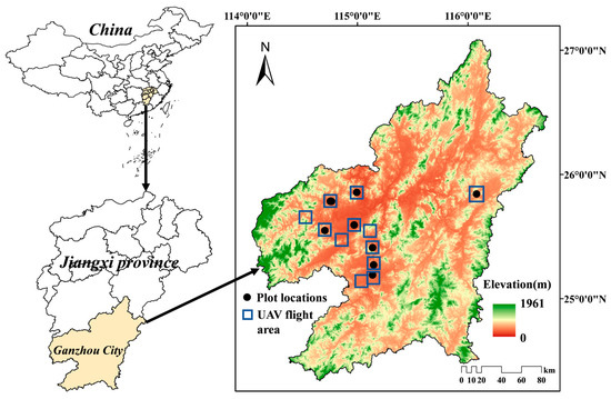
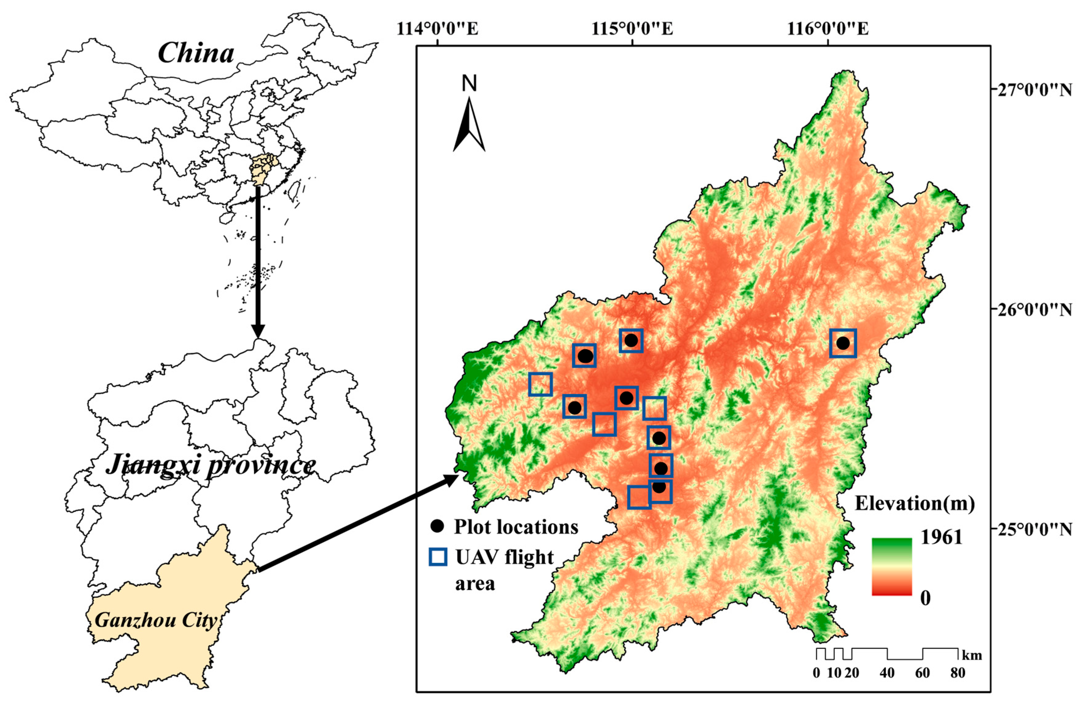
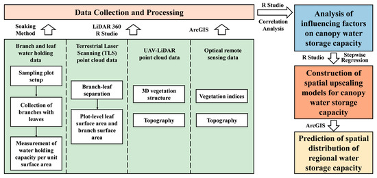
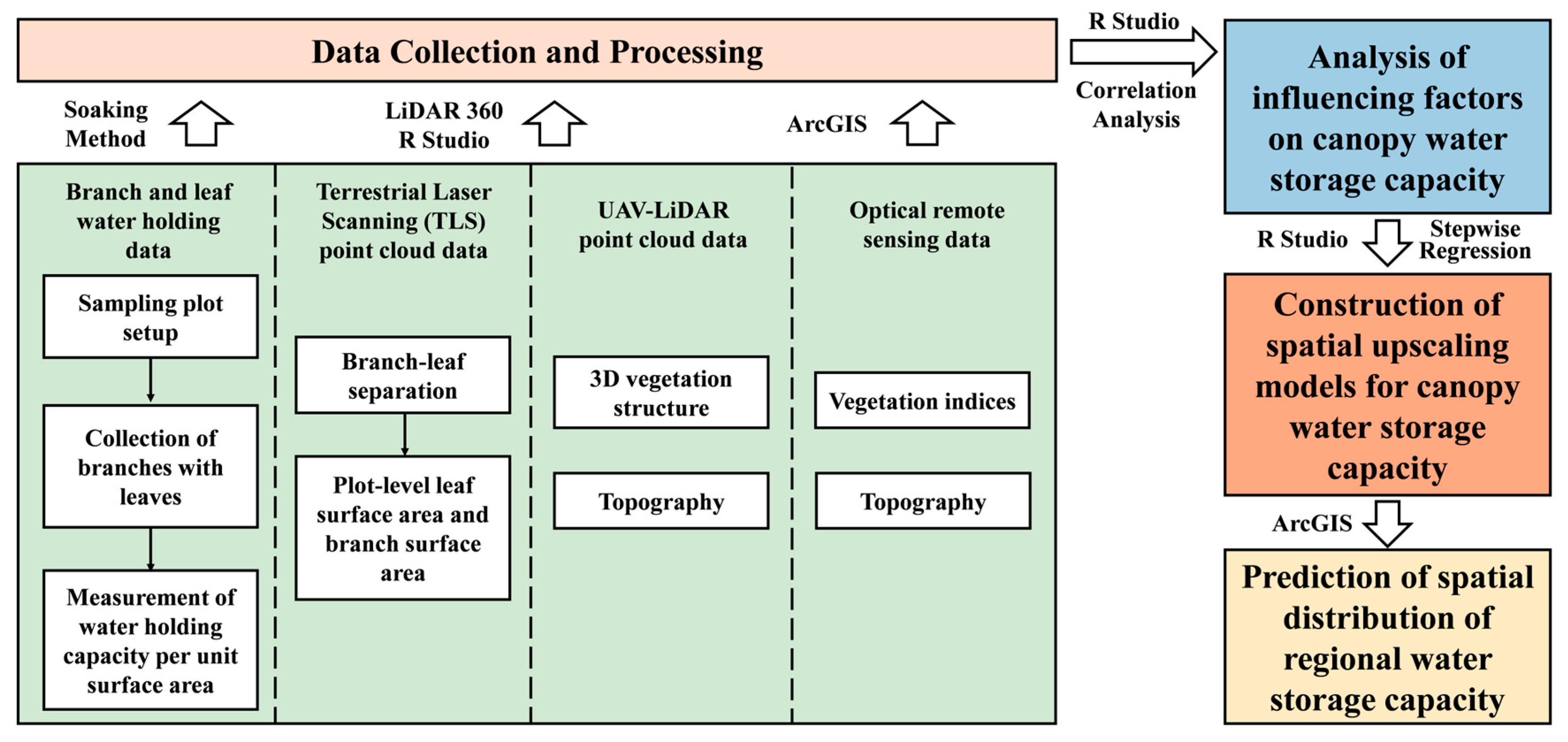
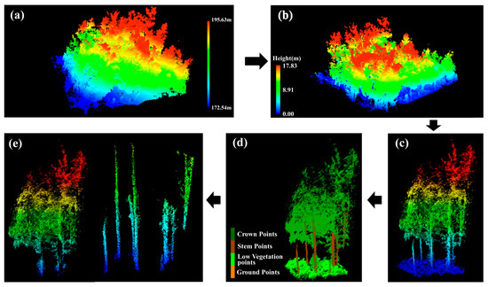
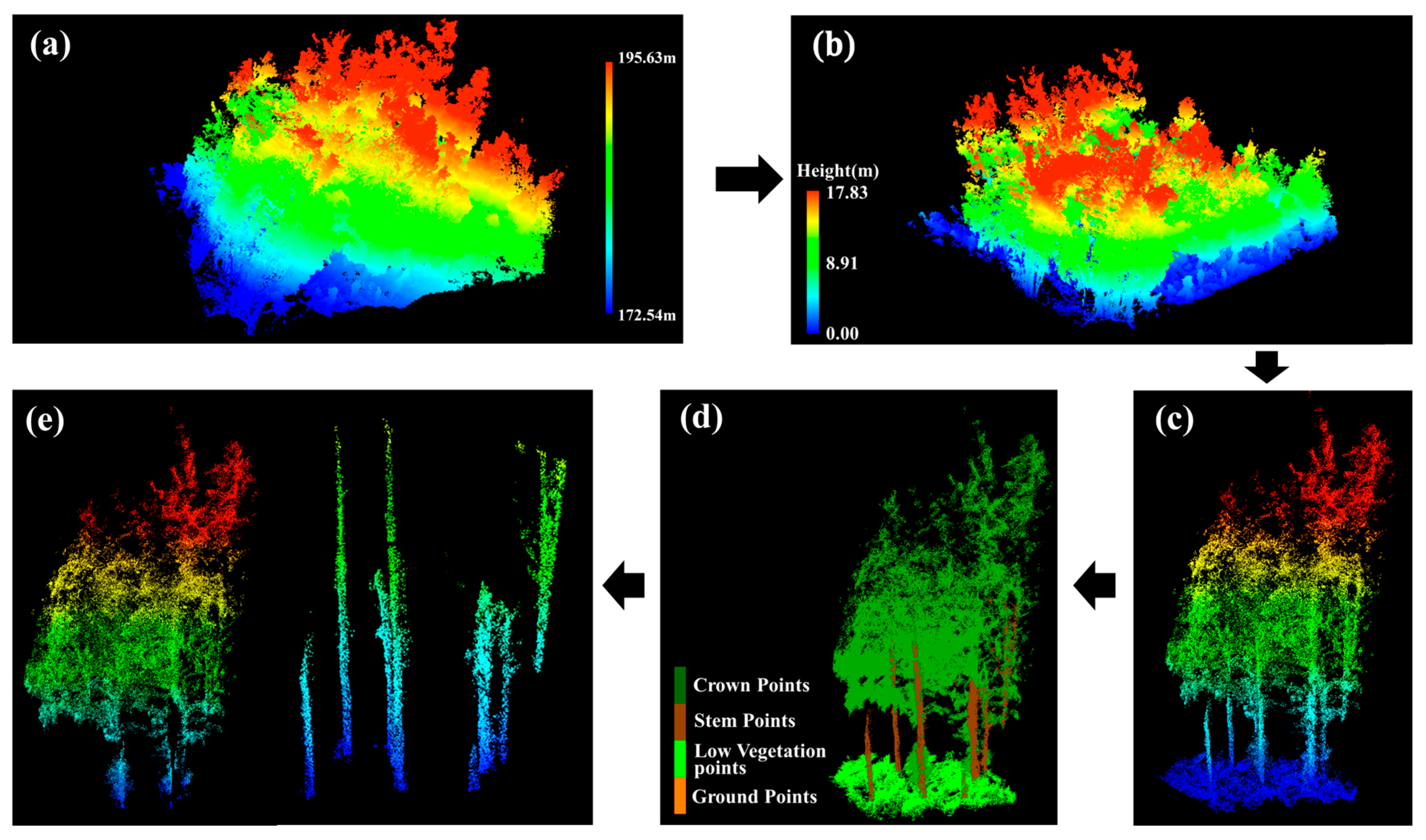
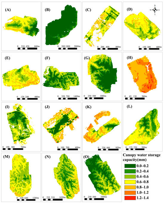
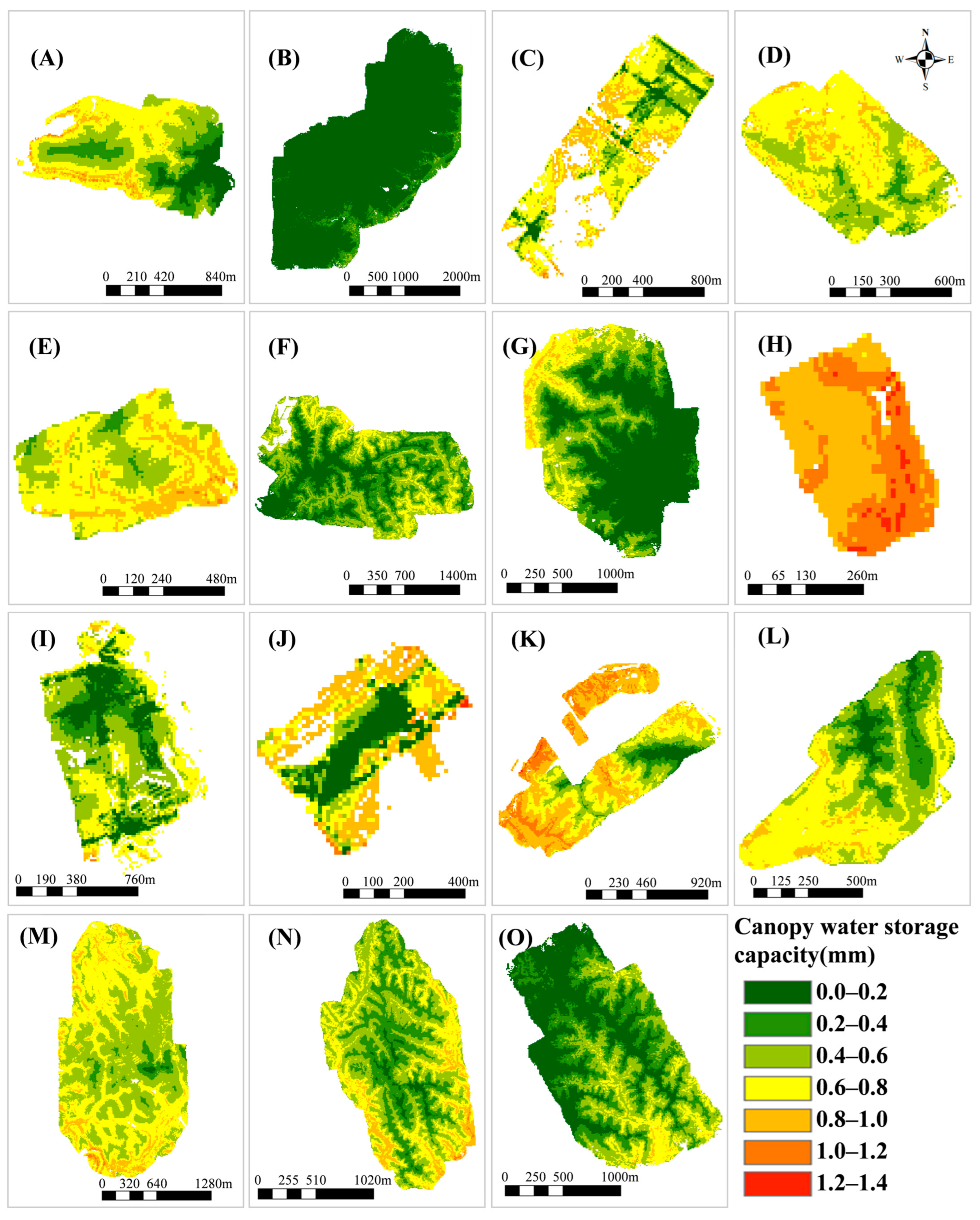
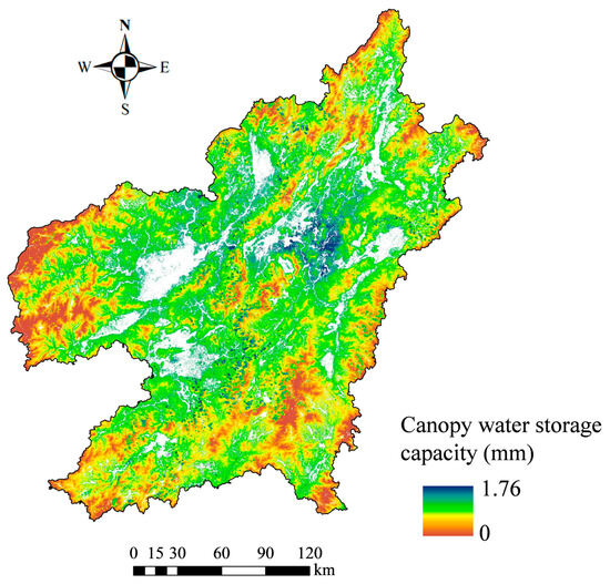
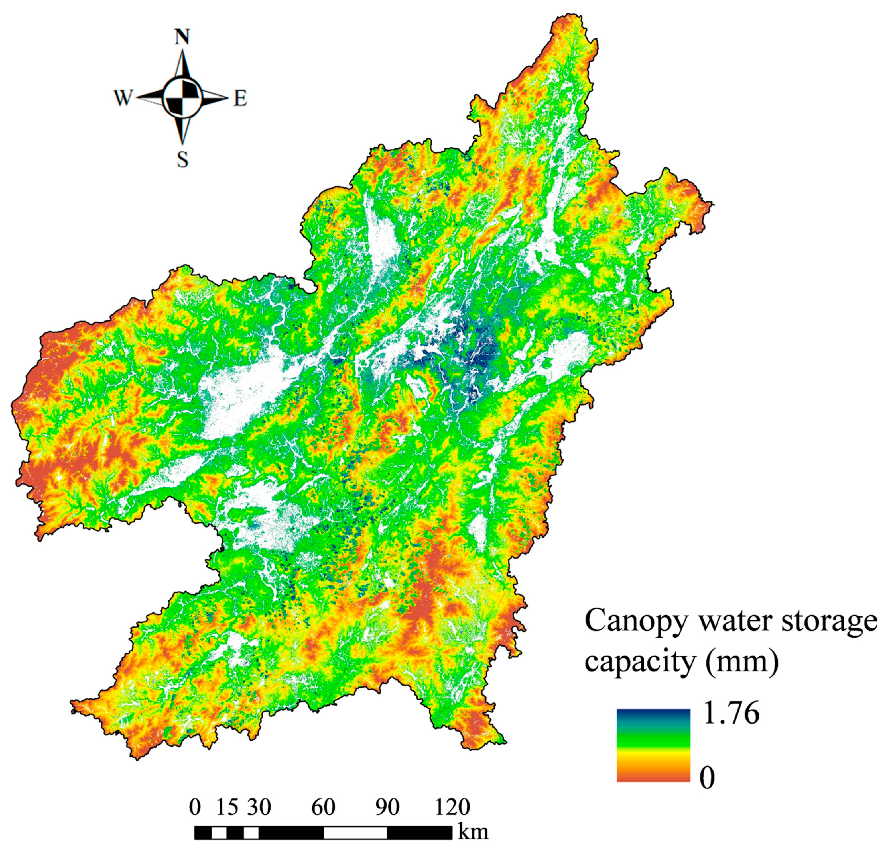
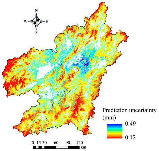
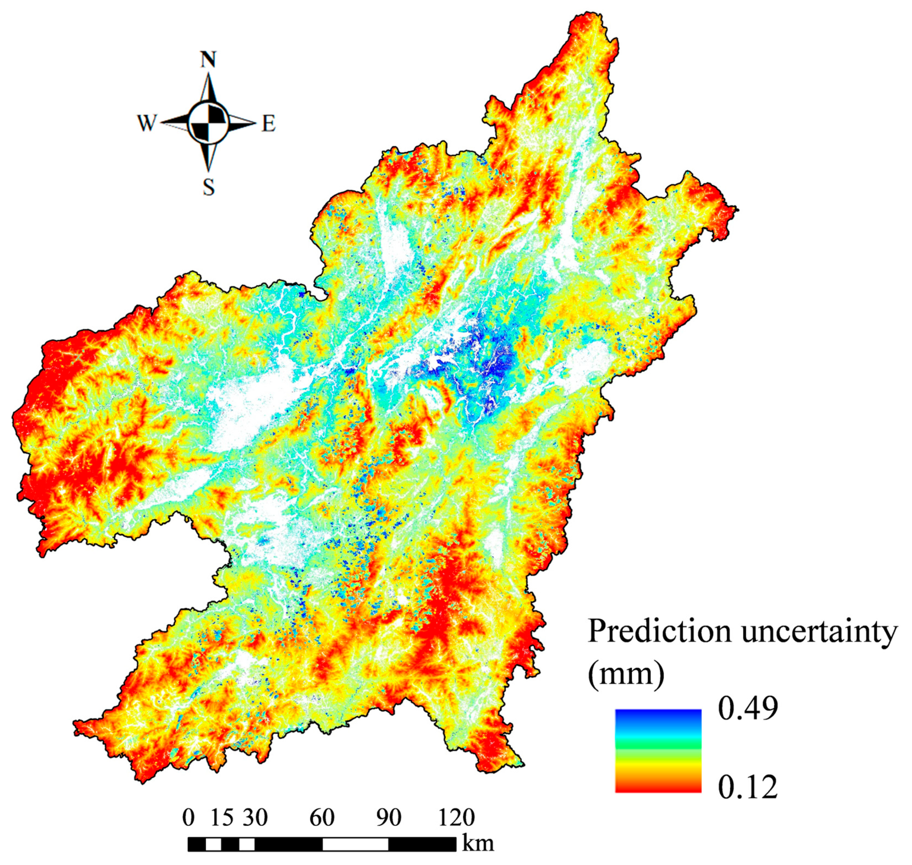
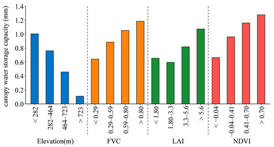

Disclaimer/Publisher’s Note: The statements, opinions and data contained in all publications are solely those of the individual author(s) and contributor(s) and not of MDPI and/or the editor(s). MDPI and/or the editor(s) disclaim responsibility for any injury to people or property resulting from any ideas, methods, instructions or products referred to in the content. |
© 2026 by the authors. Licensee MDPI, Basel, Switzerland. This article is an open access article distributed under the terms and conditions of the Creative Commons Attribution (CC BY) license.