


Highlights
What are the main findings?
- Developed a deep learning framework for analysing and detecting anomalies from space-based global ionospheric electric field data.
- The results demonstrate a statistically significant association between ionospheric perturbations and seismic events beyond random expectation.
What are the implications of the main findings?
- The results provide a robust, data-driven framework for systematically analysing ionospheric perturbations in relation to seismicity.
- The proposed framework enables a reproducible, extensible, and statistically supported methodology for future seismic–ionospheric studies.
Abstract
Detection of pre-seismic ionospheric electric field perturbation remains an open challenge in the scientific community, hindered by methodological biases and a lack of reproducible frameworks. In this study, we investigate the existence of ionospheric perturbations associated with earthquakes by developing a deep learning framework for detecting anomalous patterns in global ionospheric electric field measurements provided by the DEMETER satellite and evaluating their statistical relationship with global seismicity. We developed an unsupervised LSTM autoencoder framework trained under a rolling-window scheme with two alternative optimisation strategies. The iterative rolling-window approach enabled the preservation of long-term temporal continuity while adapting to the non-stationary ionospheric background. Anomalies detected by the model were subjected to a seismic association and evaluated statistically. Findings were consistent across multiple network configurations, independent training optimisation strategies and different segments of the dataset, demonstrating strong methodological robustness. Our study suggests that modern sequential deep-learning models, when combined with an adaptive temporal training approach and statistical evaluation, provide an effective tool for the systematic detection and statistical quantification of associations between ionospheric electric field perturbations and seismic events.
1. Introduction
Earthquakes remain among the most devastating natural hazards, with a significant impact on human populations, infrastructure, and the economy worldwide [1,2]. When tectonic plates move relative to each other at faults, they build up strain energy that is suddenly released. This creates seismic waves that travel through the Earth’s crust and cause severe damage to infrastructure and loss of life [1,3]. As we cannot prevent earthquakes, our optimal course of action is to identify reliable prior indicators of their occurrence and use them to take precautionary measures that minimise their impact.
The quest for seismic precursors has been a main area of interest for the scientific community for a very long time. The ionosphere has always been considered a crucial medium for the detection of seismic precursor signals, and its prominence has grown significantly with the introduction of continuous global monitoring by using satellites like DEMETER, Swarm, and CSES alongside terrestrial GNSS arrays, ionosondes, and ground-based VLF/LF radio signal propagation measurements, which collectively provide the extensive measurements necessary for systematic earthquake precursor investigations. Numerous studies have utilised these monitoring sources to examine ionospheric anomalies associated with pre-seismic events. Foundational statistical validations using ground-based GPS TEC and ionosonde observations established the basis for seismo-ionospheric research [4,5,6,7]. Subsequent satellite missions have allowed for systematic investigations of seismo-ionospheric phenomena. The DEMETER mission provided in situ measurements of ion density and electromagnetic variations, which have been widely used to identify potential pre-seismic signatures [8,9]. More recently, the CSES mission has facilitated detailed analyses of ionospheric electric field perturbations [10,11,12], while the Swarm constellation has supported the exploration of large-scale ionospheric disturbances potentially related to seismic activity [13,14,15]. In parallel, ground-based VLF/LF radio signal propagation measurements have provided statistical evidence of lower ionospheric perturbations [16,17]. Large-scale GNSS-based studies, using total electron content (TEC) observations [18,19,20,21], and GNSS Reflectometry and GNSS Radio Occultation data [22,23] have further contributed to the investigation of ionospheric anomalies associated with earthquakes. Additionally, multi-instrument approaches combining GNSS, CSES, and Swarm data have enabled more comprehensive analyses of such ionospheric disturbances [14,24]. Recent multi-parameter observational studies have also provided valuable insights into lithosphere–atmosphere–ionosphere coupling (LAIC) mechanisms [25,26].
During the last few decades, many studies have focused on the investigation of seismic responses in electromagnetic (EM) observations. Seismic responses in EM observations have been extensively studied across various frequency bands. Foundational work established the LAIC framework [27,28] and the theory of seismic electric signals [29,30]. Subsequent studies have explored ultra-low frequency (ULF) emissions [31,32], VLF/HF radio signals [33], non-linear dynamics of candidate electromagnetic precursors [34,35], and fracture-induced electromagnetic emissions [36]. DEMETER was the first satellite purpose-built to probe seismic and volcanic activity from space, providing uninterrupted global monitoring of the ionosphere [37]. The studies carried out by the sensors measurements of the DEMETER satellite further provide evidence for upward propagation of EM signals generated near the Earth’s surface to the ionosphere [28,29]. Despite these interesting observations, the EM precursors are still a highly disputed topic among scientists. Some studies have been carried out that argue EM precursors cannot exist [36]. The majority of these disagreements arise from an incomplete understanding of the physical mechanisms behind seismic-related EM generation phenomena, despite numerous proposed hypotheses, including atmospheric gravity wave mechanisms [38,39], solid-state physics approaches [40], radon-emission-based hypotheses [41], electric field generation in stressed rocks [42], ULF magnetic field variations [43], and mathematical frameworks of critical dynamics [44]. These debates are further shaped by the fact that most studies are centred on two strands: detailed case studies of individual earthquakes and large-sample statistical analyses of pre-seismic ionospheric conditions. In addition to these conceptual challenges, the practical methodological issue further hinders progress. Despite decades of investigation, no single EM signature has proved uniformly reliable as a precursor. The primary explanation for this lies in the methodological limitations of the approaches used in these studies, including arbitrary spatial and temporal windows, a near-epicentral data bias, hypothesis-driven methods, and limited global coverage. In many cases, precursor candidates are drawn from post hoc analyses of only a few large earthquakes, leaving statistical power and reproducibility in doubt.
Beyond simply establishing statistical correlations under a biased data sampling approach, progress in this field needs data-driven frameworks that can operate without following any prior hypothesis and can generalise across diverse tectonic and ionospheric conditions [45]. From this perspective, detailed time series analysis of EM signals aimed at uncovering complex temporal patterns expected to be induced by seismic events is considered particularly important. Bridging this gap will require harmonised data coupled with transparent, data-driven algorithms that can generalise across different tectonic settings. The rapid advancement of artificial intelligence (AI), spanning deep learning (DL) and generative AI, has enabled the successful accomplishment of tasks that were once unfeasible or totally impossible in recent years. Over the past few years, researchers have begun to explore ML and DL methods to pick out anomalous ionosphere signatures that may indicate an impending earthquake. Early efforts utilised conventional ML approaches such as support vector machines (SVM) [46], while subsequent research applied DL techniques including convolutional neural networks (CNNs) [47,48,49]. Although DL for electromagnetic-based precursors remains less explored, recent studies have demonstrated its growing capability using DEMETER [50], Swarm [51], GNSS [52], and multi-parameter data [53]. As reviewed by [54], DL architectures have evolved from basic feedforward neural networks to complex models such as CNNs, recurrent neural networks (RNNs), and generative adversarial networks (GANs), demonstrating increasing capability in finding critical seismic-related perturbations, though challenges in accuracy and interpretability persist [54].
The specific contributions of this work are fourfold. First, we adopt a global anomaly-first approach that detects ionospheric anomalies from global ionosphere electric field observations independently of earthquake information, allowing us to subsequently test their statistical association with seismic occurrence without imposing a priori causality. Second, we develop a rolling-window training framework that iteratively adapts to evolving ionospheric conditions, validated across a primary phase (2005–2009) and a blind phase (2010), addressing the challenge of generalisability in deep learning applications for this domain. Third, we conduct a systematic exploratory screening of spatial and temporal labelling criteria without presuming any existing physical coupling model. Fourth, we evaluate robustness and sensitivity across different model configurations and training strategies. Section 2.1 provides a detailed explanation of the data and preprocessing procedures used in this study, followed by Section 2.2 outlining the DL architecture and statistical evaluation framework. Section 3 presents the model-based results and analysis. Section 4 discusses the main findings of the study, while Section 5 summarises the work and outlines directions for future research.
2. Materials and Methods
2.1. Data and Preprocessing
The primary data utilised in this study are ionospheric electric field power spectrum density (PSD) data obtained from the Instrument Champ Électrique (ICE) flown on the French CNES microsatellite DEMETER [55]. The DEMETER mission was targeted to monitor ionospheric perturbations potentially associated with lithospheric processes [37]. The satellite, carrying instruments onboard measuring electromagnetic waves, plasma parameters, and energetic particles, operated on a polar, nearly circular orbit at an altitude of 715 km (lowered to 660 km after 2005), with a slow drift in local time, crossing the equator around 10:30 LT during the day and 22:30 LT at night. The measurements are limited to latitudes below approximately 65° invariant latitude and are operated in two modes, a survey mode for continuous low bit rate data collection and a burst mode for high bit rate measurements in seismically active regions [37]. The ionospheric electric field data analysed were recorded by DEMETER in the very low frequency (VLF) band during survey mode, captured with a frequency resolution of 19.5 Hz and a time resolution of 2 s, resulting in approximately 57,839 half-orbit records from 2004 to 2011.
Data processing involved a series of systematic steps designed to ensure the integrity, consistency, and analytical suitability of the datasets. Initial preprocessing included data cleaning, grid segmentation, feature extraction, time series construction, and background correction. The analysis concentrated on six years of DEMETER observations (2005–2010), with data from 2004 and 2011 excluded due to mission setup anomalies and end-of-mission irregularities that compromised data quality. Some orbit files had very unusual sizes, which, on investigation, were found to result from missing data points or atypical orbital coverage, and these files were also excluded. Incomplete orbits were also removed to ensure consistency across both daytime and nighttime datasets. Consequently, the final dataset comprised 26,276 complete orbits, resulting in 52,552 half-orbit VLF spectrograms for subsequent analysis. All the primary data cleaning steps are provided in Table 1. No explicit filtering based on geomagnetic activity indices (e.g., Kp or Dst) was applied in the current study. To ensure a homogeneous ionospheric baseline and avoid the elevated VLF variability characteristic of nightside conditions, the analysis is restricted to the 26,276 daytime DEMETER orbits. This selection reflects a deliberate effort to maintain physical consistency, as daytime and nighttime ionospheric conditions represent distinct regimes in terms of VLF propagation, D-layer behaviour, and background electron density variability. Combining these regimes within a single framework would introduce systematic inconsistencies in the anomaly detection process. Accordingly, the present study focuses on the daytime ionosphere as a well-defined and internally consistent domain. Extending the framework to nighttime conditions as a separate analysis remains a direction for future work.
Table 1.
Summary of quality-control filters applied to orbit files.
The major preprocessing step consisted of transforming the PSD data into time series data, keeping the spatial referencing. This is achieved through a grid-based segmentation approach, wherein the Earth’s surface is partitioned into cells measured 20° in both latitude and longitude. Each grid cell was uniquely identified to enable the spatial mapping of spectral measurements. By this, the electric field PSD data recorded at regular intervals of time can be mapped to their corresponding geographic locations. For feature extraction, 11 logarithmically spaced frequency bands below 3 kHz were selected, encompassing the extremely low frequency (ELF, 3–3 kHz) ranges as defined in Table 2, following the study by [50].
Table 2.
Frequency bands derived from ICE PSD measurements.
For each daytime orbit, we sample the data every 2 min, and at each interval, a spatial range of a 10° × 10° square is considered around the orbital footprint, as illustrated in Figure 1. From the spectrum within this spatial range, the quartile feature Q3, defined as the 75th percentile of the PSD, is derived from the predefined 11 frequency bands, yielding 11 features every 2 min. Each resulting feature vector is then assigned to the grid that has the largest overlap with the corresponding 10° square. The following Figure 2 is the comparison of the raw PSD data (see Figure 2a) of a randomly picked daytime orbit and the transformed time series data across 11 frequency bands below 3 kHz (see Figure 2b). The total duration of the orbit is 34 min, which, when resampled every 2 min, provides a 17-point series. These data points are associated with different grid cells along the orbital passage. Finally, each of the grid cells is associated with discrete time series data spanning six years, the duration of the study. An illustrative example of the temporal evolution of Q3 in grid cell G42 over six years for frequency band FB5 is provided in Figure 3. Each of the grid data exhibits some intrinsic periodical fluctuations and trends that need to be addressed separately, considering its geographic constraints.
Figure 1.
The figure illustrates the path of the daytime orbit. The blue dots represent the orbit’s position at every 2 min interval, where spectral features (quartile feature Q3) are calculated within the area of the red squares.
Figure 2.
DEMETER electric field measurements for orbit 03232_0. (a) Electric field PSD of a daytime half-orbit (19.3 Hz–18 kHz). (b) Derived Q3 time series for 11 frequency bands below 3 kHz, resampled at 2 min intervals.
Figure 3.
The time series data of grid cell G42 for the frequency band FB5. The evolving trend and periodic fluctuations illustrate the intrinsic variability of the ionosphere electric field over the given geographic location.
Although the study adopts a global framework, the term “global” in this context refers to the absence of region-specific selection (e.g., focusing on individual earthquake zones) rather than uniform spatial coverage of the entire Earth. The DEMETER satellite provides quasi-global longitudinal sampling; however, its measurements are constrained to invariant latitudes. As a result, high-latitude and polar regions are absent from the dataset, and the analysis primarily reflects low- and mid-latitude ionospheric behaviour. The grid-based system is introduced to spatially organise the spectral observations into geographically referenced time series. Each grid represents a distinct geographic region for which localised ionospheric variability can be analysed. This approach enables the construction of geographically resolved time series that preserve spatial context and allow for region-specific background correction and trend estimation. There are 162 grid locations globally, with each half-orbit intersecting approximately 145 of these grids. The grids located poleward of ±65° geomagnetic latitude were largely unpopulated, consistent with the satellite’s invariant orbital constraints. Therefore, the results should be interpreted as geographically distributed but spatially non-uniform, reflecting the effective observational coverage of the DEMETER daytime orbits.
The second set of data utilised in this study for the investigation of seismic correlation is a global earthquake catalogue spanning a period of 6 years from 2005 to 2010. The data was provided by the ANSS Comprehensive Earthquake Catalogue (ComCat) maintained by the U.S. Geological Survey [56]. This catalogue provides global hypocentre location and magnitude solutions (Mw) for events detected since the early twentieth century. In this study, we limit our analysis to earthquakes with a magnitude of 5 Mw or greater. In total, approximately 12,000 earthquakes were globally available for the study. Table 3 summarises the key characteristics of the datasets employed in this study.
Table 3.
Summary of datasets used in this study.
2.2. Methodology
The study adopts a structured data-driven framework. Unlike the conventional workflow, where the dataset is split into fixed-period subsets of training and validation intervals, we employ a temporally adapting approach considering the non-stationary time-dependent behaviour of ionosphere electric field data. To preserve temporal consistency and to avoid the artefacts caused by the conventional methods, we introduce an iterative rolling-window design. This framework forms the basis of all the subsequent analyses and performance assessments presented in the study. The overall workflow of the proposed methodology is illustrated in Figure 4. This study follows a structured two-stage data-driven framework. First, both the ionospheric data and the earthquake data are collected, and the ionospheric measurements are then preprocessed using grid-based segmentation to generate time series representations, which we have already discussed. In the second stage, a rolling-window methodology is applied to account for the non-stationarity of the data. This stage integrates background correction, model training, and statistical evaluation within two phases: a primary phase and a blind phase. A detailed description of each component of the methodology is provided in the following sections.
Figure 4.
End-to-end workflow of the proposed methodology. Color coding indicates functional grouping: the red shaded region denotes that all enclosed processes are performed within the rolling-window framework. Blue boxes represent the analysis phases following the methodology described.
2.2.1. Rolling-Window Design
The temporal continuity is preserved by the rolling-window framework by partitioning the six-year data into overlapping 15-month segments. Each window consists of 12 months of training data and is followed by the 3 months of the validation set. Each of the windows is indexed sequentially as . After each iteration, the window advances by three months, creating a total of 20 windows across the study period. Within each window, the training segment is used solely for model training, while the validation segment is used for independent anomaly detection evaluation (elaborated in Section 2.2.4). It is important to note that all model performance evaluations are derived from the anomaly detection results on this full 3-month validation segment of each window. Thus, the full validation segment, therefore, serves the functional role of an independent test set in the conventional sense: it is data on which no training was performed, no hyperparameters were tuned, and on which all reported performance metrics are computed.
The 20 windows are further divided into two analysis phases. The primary phase comprises windows to , whose validation segments span 2005 to 2009. This is the primary phase of modelling, where the model is trained iteratively on the training data of each window and tested on the corresponding validation segments. This phase is used for primary statistical evaluation and criterion selection (see Section 2.2.3) based on the model’s performance on the validation data. The blind phase analysis comprises windows to , whose validation segments cover January to December 2010. In the blind phase, training continues in the same rolling fashion; each blind window retrains the model on corresponding training data to accommodate the evolving ionospheric background, but the validation data on which performance is evaluated is entirely new and was never encountered at any stage of the primary phase, including training, validation, or criterion selection. Thus, the independence of the blind phase is ensured in three ways. First, within every blind window, the validation segment on which all anomaly detection results and statistical evaluations are computed is data that the window’s model has never trained on. Second, none of the four 2010 validation segments were used in any training or evaluation step during the primary phase, which concluded with whose validation covered only up to December 2009. Third, the best-performing spatio-temporal criterion and model architecture were all fixed from primary phase results before any 2010 data was encountered in any form. The blind phase analysis, therefore, demonstrates the generalisability and practical applicability of the rolling-window training strategy when new data becomes available beyond the primary study period, simulating a realistic operational scenario where the model continuously adapts to recent ionospheric background conditions and is evaluated on the next unseen period.
The background correction of data also follows the same method. Thus, this design allows the model to be trained iteratively on evolving segments of data, enabling continuous adaptation to time-transient ionospheric conditions and providing a more realistic performance assessment framework. Figure 5 is the schematic representation of the rolling-window strategy. Each square represents a 3-month interval, with the blue segment denoting the training data segment and the orange representing validation within the given iteration. The first iteration uses , the training segment for fine-tuning and optimisation of the model, and the following three months for validation. This process is repeated across all 20 windows, resulting in 20 sequential training–validation cycles. The final year [2010], marked by a grey stripe, is kept as a blind set for later analysis.
Figure 5.
Schematic representation of the rolling-window design: each window spans 15 months (12 months training, 3 months validation) with a 3-month step. Windows 16–19 are reserved as blind tests.
2.2.2. Iterative Background Fitting
Before the modelling phase begins, the data undergo a background correction aimed at removing intrinsic trends and periodic fluctuations that may interrupt the detection of meaningful anomalies by the model at the grid level. The major aspect of the background correction in this study is that it follows an iterative nature. For each rolling window, the background curve is fitted using all available data from the beginning of the study (1 January 2005) to the start of the corresponding validation period. This ensures that each new fit incorporates the cumulative background information from previous time intervals, thus allowing the model to continuously enhance its understanding of the long-term background behaviour. This iterative improvement enhances continuity between consecutive windows, reducing discontinuities that might otherwise arise from independent fitting operations. To address the periodic nature and trend, the background behaviour of the data is represented by a function that combines a linear and a sinusoidal component. The linear term models the slow trends over time, while the sinusoidal term captures the repeating periodic variations in the system. The general form of the background function can be expressed as,
where a denotes the constant offset representing the mean background level, b is the coefficient of the linear trend accounting for slow drifts, c represents the amplitude of the periodic component, d defines the period of the cycle which is fixed as 1 year, and e is the phase shift. The background estimate is derived from data resampled at 30-day intervals. During resampling, the mean is computed using only the values that fall within the 90% confidence interval of the resampled data, ensuring that outliers are excluded from the background calculation. The background coefficients are first estimated using the resampled data and then fitted to the full dataset. The fitted background curve is then subtracted from the original dataset to produce the background-corrected residuals.
A key feature of the background correction procedure is that it operates on spatially segmented, grid-based data. Each grid cell corresponds to a separate six-year dataset, within which the rolling-window background correction is performed independently. The eleven frequency-band dataset of each grid cell undergoes iterative background correction independently. This allows region-specific seasonal cycles and long-term trends to be accounted for without imposing a uniform global correction. Geomagnetic activity, solar influences, and other external electromagnetic sources are not explicitly filtered at this stage. This choice prioritises an unbiased representation of the ionospheric variability, enabling the model to learn background behaviour directly from the data. While Figure 3 shows the full six-year data for a given grid and frequency band, where periodicities are clearly visible, Figure 6 illustrates the window-based background correction for window as a representative example. To provide sufficient temporal context for the periodic structure to be visually appreciable, the figure displays the extended period spanning windows through (April 2008 to January 2011). The blue scatter represents the raw Q3 measurements, the black dots represent the 30-day resampled data, and the black curve represents the fitted background function. The sinusoidal nature of the fitted curve is clearly visible across the extended display period, demonstrating that the background model successfully captures the repeating annual cycle present in the ionospheric electric field measurements. Consistent with the rolling-window training strategy, the background estimation and curve fitting for are performed excluding the validation segment (October 2010 to January 2011). The residuals (red scatter), shown on the right axis with the dashed grey line marking zero, are obtained by subtracting the fitted background from the raw data across the full window period. The fitted curve explicitly combines a linear trend and an annual periodic component. The estimated linear slope is approximately −0.107 per year, which is small relative to the short-term variability and therefore not visually dominant. In contrast, its oscillatory behaviour associated with the annual component is now visually identifiable in the figure. The residuals, shown on the right axis, are centred around zero (mean ), confirming that the background subtraction effectively removes the dominant trend and periodic components. The observed asymmetry in the residual distribution, with some points deviating substantially in the positive direction, is a deliberate consequence of the background estimation strategy: by excluding extreme values from the resampling, genuine anomalous deviations are intentionally preserved in the residuals rather than absorbed into the background estimate. This ensures that potential strong ionospheric perturbations are not suppressed during preprocessing, providing an anomaly-sensitive input for the subsequent deep learning detection step. Finally, when all the residual data from each grid cell is combined, it forms a complete dataset, which is then segmented according to the rolling window.
Figure 6.
Temporal evolution of the quartile feature Q3 for grid cell G42, frequency band FB5. The extended period (April 2008 to January 2011) is shown to make the annual periodic structure visually appreciable, while the background correction is applied specifically to window . Blue dots show the raw measurements, black dots show the 30-day resampled background estimates, and the black curve shows the fitted background combining a linear trend and an annual sinusoidal component, estimated excluding the validation segment of . Red dots show the background-corrected residuals (right axis), with the dashed grey line marking zero. The residuals are centred around zero, confirming effective removal of the dominant trend and periodic components, while extreme positive deviations are deliberately preserved as potential anomalous signals.
2.2.3. Space–Time Seismic Criteria
Transforming the data into a suitable input for the machine-learning or DL models is a critical step. In this study, we use two consecutive daytime half-orbits as a single input sample (also called “sequence”). From a physical perspective, each DEMETER half-orbit represents a continuous latitudinal transect, providing an idea of the ionospheric state along the orbital path. Using two consecutive daytime half-orbits allows the models to capture a broader temporal evolution of ionospheric conditions while maintaining consistency in local time sampling. Since we are not adhering to any established hypothesis about ionosphere–lithosphere coupling, we do not have a predefined expectation of when or where, before an earthquake, such anomalies, if they exist, might appear [57]. Given that current knowledge about the existence and propagation of these signatures is limited and not completely accepted by the scientific community, we systematically explore a wide range of spatial and temporal windows.
The data measurements are available every 2 min, so the spacecraft position along the orbit is sampled at 2 min intervals. By using two consecutive daytime half-orbits as inputs, we effectively consider a spatial window (SW) surrounding the orbital footprint along the entire orbit, within a time window (TW) that starts after the end of the second half-orbit. In this sense, we search the past ionospheric data for the anomalies that can later be tested for correlation with earthquakes occurring in the future. The first part of the study requires the model to learn the expected nominal behaviour of the ionospheric electric field signal. For that, we classify the input orbit samples into “seismic” or “non-seismic” using a set of spatial–temporal window configurations. In the first part of the modelling, we combine these different spatial windows with a fixed temporal window of 48 h. Table 4 provides the naming convention and a detailed description of each spatial window (spatial range defined similarly to the representation in Figure 1).
Table 4.
Spatial window definitions used for seismic/non-seismic classification (TW = 48 h fixed).
After identifying the best-performing spatial-window category, we perform a time-window analysis using several temporal windows (TW) of 6, 12, 24, and 48 h. Each combination of SW-TW is treated as a separate criterion and is evaluated with the same deep-learning pipeline. This two-stage screening is designed to identify which data partitioning, governed by the spatial and temporal window, produces the most consistently learnable representation of nominal ionospheric behaviour across models, rather than to maximise a post hoc correlation parameter. The choice of spatial and temporal window is not merely a statistical tuning parameter; it fundamentally determines the classification of input orbits into seismic and non-seismic categories, and therefore directly controls the composition of the training dataset. A narrower spatial window results in fewer orbits being labelled as seismic, thereby preserving a larger pool of non-seismic data for learning nominal behaviour. In contrast, a wider window increases the number of seismic-labelled samples, reducing the available training data accordingly. Each spatial–temporal criterion therefore yields a distinct model trained on a different data composition. Since no prior consensus exists in the literature regarding the spatial and temporal scales of pre-seismic ionospheric perturbations, systematic exploration of a physically motivated set of configurations is the methodologically appropriate approach. The selected criterion from the primary phase of training and analysis is subsequently applied unchanged to the blind phase, providing independent temporal validation of this choice on data entirely withheld from the selection process.
2.2.4. Deep-Learning Framework: LSTM Autoencoder
The ionosphere is a temporally evolving environment in which anomalous signatures, if present, manifest as deviations from learned sequential patterns. This makes deep learning particularly well-suited to unsupervised anomaly detection, as it can capture complex temporal dynamics directly from data without requiring explicit physical model assumptions. We adopt an LSTM Autoencoder architecture for this purpose. The LSTM, introduced by Hochreiter and Schmidhuber [58], is designed to learn long-term temporal dependencies in sequential data through gating mechanisms that regulate information flow, making it well-suited to modelling ionospheric time series where dependencies extend across 30–40 min of orbital observations. Autoencoders are a class of neural networks designed for unsupervised learning tasks, specifically to learn efficient representations of data [59]. An autoencoder is composed of an encoder–decoder architecture that learns the underlying data representation by compressing it to a latent space and reconstructing it back to the original input. By constraining the reconstruction to start from a reduced dimension, the model is forced to learn only the salient features of the training data [60]. Model performance is assessed through the reconstruction error, the difference between input and output, where a larger error indicates that the input diverges from what the model has learned to represent. When trained exclusively on nominal ionospheric conditions, the autoencoder functions as an effective anomaly detector, since inputs that diverge from the learned normal patterns yield significantly higher reconstruction errors [61,62]. This unsupervised design is a deliberate methodological choice. Because the model is trained only on background ionospheric data with no seismic labels forcing to learn the complex and inherent patterns within the background data for better detection of anomalies.
By combining LSTMs with an autoencoder architecture, we aim to exploit both the long-term temporal dependency learning and latent-space reconstruction for anomaly detection. Many advantages of using this combination for unsupervised anomaly detection are explained by [60,63]. Our proposed architecture comprises stacked LSTM layers in both the encoder and decoder layers. Such a network trained only on nominal data can be used for anomaly detection in multivariate time series [62]. In our case, the LSTM autoencoder is trained solely on the non-seismic category of data and therefore learns to reconstruct better nominal ionospheric behaviours. If the seismic category of data contains structures of complex patterns that deviate from learnt background patterns, the model struggles to reproduce them and can flag such cases as anomalies through a higher value of reconstruction error. Thresholding this reconstruction error allows us to automate the classification of anomalous behaviour. Similar strategies have been successfully applied in previous anomaly detection studies, including [60,64,65].
The proposed network follows an encoder–decoder topology, as illustrated in Figure 7. Figure 7a presents the parallel training and optimisation strategy employed in this study. As discussed in Section 2.2.3, each input sample consists of two consecutive daytime half-orbit time series, denoted as and . To preserve orbital continuity while avoiding artefacts associated with direct concatenation, the two half-orbits are processed independently through identical LSTM autoencoder branches. The corresponding reconstruction losses, and , computed using the mean squared error (MSE), are averaged to form the final loss used for backpropagation. This arrangement of training keeps the joining point of orbits from dominating the loss, yet still preserves the benefit of presenting neighbouring trajectories together.
Figure 7.
Overview of the LSTM autoencoder framework. (a) Parallel LSTM autoencoder architecture used for electric field anomaly detection, where each half-orbit input is processed independently and the average reconstruction loss is used for optimisation. (b) Detailed LSTM autoencoder architecture. The input time series with features F and timestamps T is encoded into a latent vector of dimension Z, which is repeated across the temporal dimension and passed to the decoder for sequence reconstruction.
Figure 7b illustrates the internal architecture of the LSTM autoencoder. Each input sequence represents a multivariate time series with a fixed temporal length of and features. The input is passed through an encoder composed of two stacked unidirectional LSTM layers, which progressively compress the temporal information into a latent representation. The final hidden state of the encoder is projected through a fully connected linear layer to a low-dimensional bottleneck of size . To enable sequence reconstruction, the latent vector is repeated across the temporal dimension and fed into the decoder, which mirrors the encoder structure with two stacked LSTM layers followed by a linear output layer. The decoder reconstructs the original input sequence .
Training minimises the mean-squared reconstruction error calculated by the loss function (2), where and denote the input half-orbit sequence and output of the autoencoder, respectively. Mean squared error is defined as the average of the squared differences between the output and input values [66]. Optimisation was performed using the Adam (learning rate , batch size = 8) training set for 1500 epochs with an early-stopping patience of 100 epochs [67]. Model training relied exclusively on nominal, non-seismic records selected according to the screening criteria detailed in Section 2.2.3. Data normalisation was performed using a standard scaler fitted solely on the training dataset. The deep learning models were implemented in Python (version 3.11) using PyTorch (version 2.1). Table 5 provides a summary of the LSTM autoencoder architecture and the key training hyperparameters used in this study.
Table 5.
Summary of the LSTM autoencoder architecture and training hyperparameters.
We trained several configurations of autoencoders with a set of different LSTM hidden dimensions while keeping all other hyperparameters fixed. Two iterative learning strategies were explored under the rolling-window framework. In the weight-updating mode (named ‘A’, …), the model weights obtained from one window initialise training in the subsequent window. In contrast, the re-initialised mode (named as ‘In-A’, …) resets the model weights for the training of every window, ensuring independent learning for every iteration. Table 6 summarises the mode of training, the naming, and its corresponding set of hidden dimensions used for the study. For each set of data prepared under the spatial–temporal criterion specified in Section 2.2.3, the corresponding training is carried out separately. In effect, for every spatio-temporal criterion, the model is trained in two optimisation modes across five different network configurations, iteratively over the 20 rolling windows, constituting the primary phase of analysis and blind phase analysis, characterising the framework’s behaviour and generalisability under the chosen spatio-temporal criterion.
Table 6.
LSTM autoencoder models and training modes.
The model training is a two-stage process within each window that ensures strict separation between model learning and performance evaluation at every step. In the first stage, the model is trained exclusively on the non-seismic portion of the 12-month training segment. Orbits classified as seismic under the chosen spatio-temporal criterion are removed from the training data entirely, ensuring the model learns only the nominal background behaviour of the ionospheric electric field. The generalisation capability of the model is assessed using the non-seismic portion of the 3-month validation segment, evaluated under the evaluation mode of the model. This monitors whether the model has successfully learned the nominal ionospheric background without overfitting to the specific training period, using data the model has not encountered during training. In the second stage, once training is complete, the model is applied to the full 3-month validation segment, including both seismic and non-seismic periods. This is the data on which anomaly detection results are computed. Since the model was trained only on non-seismic data from the training period, the entire validation segment with seismic and non-seismic data constitutes genuinely unseen data for anomaly detection purposes. This process is repeated across all 20 rolling windows, ensuring that in every iteration the anomaly detection performance is assessed on data the model has never trained on.
2.2.5. Anomaly Detection and Seismic Correlation
For each input sequence, the resulting anomaly score is defined as its mean-squared reconstruction error . This error quantifies how well the model has reconstructed the input data, with higher error representing a stronger deviation from the expected or learnt behaviour by the model. Owing to the squared formulation, large deviations are more strongly penalised than small ones, ensuring that the stronger deviation from the learned patterns contributes prominently to the error distribution [68].
For all the windows, the training segment data are used to estimate the reconstruction-error distribution and define the anomaly threshold, as this dataset represents the full extent of information available at the learning time period. The 98th percentile of this distribution is the decision threshold for anomaly detection in the validation segments (refer to Appendix A.1, Figure A1 for more details). A sequence is therefore labelled anomalous whenever its error is higher than this boundary, since such elevated error marks a sequence whose temporal structure the network is unfamiliar with. Figure 8 illustrates this procedure for the first rolling window , showing the reconstruction-error distributions for both training and validation sequences. The 98th percentile value (marked as a blue vertical line) of the training distribution is the anomaly threshold used in the study for this particular window. The validation distribution exhibits a rightward shift relative to the training distribution due to the expected increase in reconstruction error when the model is applied to the unseen data. The statistical difference between the training and validation data distribution arises from the fact that both datasets are of different durations.
Figure 8.
Reconstruction error (MSE) distribution for the training and validation sets in rolling window . The 98th percentile of the training set (blue vertical line) is used as the anomaly threshold. The X-axis denotes the reconstruction error calculated, and the Y-axis represents the number of sequences.
The anomalies detected by the model are subsequently subjected to seismic correlation analysis. For every anomaly detected by the network, we search for earthquakes occurring within the corresponding spatial and temporal window defined by the respective spatial–temporal criteria of the dataset. This yields a seismic-to-anomaly ratio, representing the proportion of detected anomalies that coincide with seismic events effectively, a true positive rate. The associated uncertainty in the ratio is quantified using the binomial error estimate. Since each input sequence consists of two half-orbits (34 data points), if at least one earthquake occurs within the specified spatial or temporal window for any point along the orbital segment, the entire sample is labelled as seismic. The model performance is evaluated based on these outputs across all the windows.
2.2.6. Random Baseline
To estimate the likelihood of obtaining a seismic coincidence purely by chance, we performed a time-randomised sampling test (noted as RST). Instead of subsampling within a specific window, we drew 200 random orbital sequences (each consisting of two half-orbits) from the full six years of data. Each sequence defines a geographic swath over which seismic association is evaluated. To avoid bias arising from the true event timing, we randomly shifted the timestep of each sampled sequence by an offset randomly selected between 5 and 30 days, thereby ensuring temporal randomisation. This means the ionospheric observation from the orbit and the earthquake search window are completely separated in time; the orbit only tells us where to look, and the shifted window tells us when to look. Earthquakes occurring within the spatial vicinity of the orbit and within this shifted time window were identified under each seismic criterion (refer to Section 2.2.3). Each sampling provides a seismic association ratio. Repeating this for 1000 trials produced an empirical distribution of the probability of random association. From this distribution, we extract the median () and the 0.3–99.7 percentile interval (0.3–99.7% RST) representing the level, which together form the random baseline used for comparison with the model-driven results.
2.2.7. Z-Factor Analysis
To assess cumulative model performances over time, we derive a meta-analytic score by averaging the values across all windows. The Z-factor reflects how strongly a given model’s seismic anomaly rate deviates from the expected random baseline. For each rolling window i, the is derived from the seismic anomaly ratio (in percentage) and its associated binomial uncertainty within the validation segment. The summary score is defined as the Z-factor ().
Since the first window of weight-updating models begins with randomly initialised parameters, it is excluded from aggregation; thus, k is 15 for updating models and 16 for the re-initialising model for the preliminary stage of analysis (models trained for the year from 2005 to 2009). Although these statistics are not Stouffer’s meta-analysis in its right form, it is interpreted through the same conceptual frame of meta-analysis [69,70].
As per the Stouffer’s method, the nominal significance is achieved in a manner analogous to standard testing, where the cumulative value (5) is compared against a chosen significance criterion ( = 2 or 3). Under our Z-factor formulation, this corresponds to
Thus, models satisfying this criterion exhibit statistically meaningful seismic anomaly association. By comparing the number of models satisfying this condition under each spatio-temporal labelling criterion, we identify the definition that yields the most consistently high-performing behaviour and use it for detailed evaluation in subsequent analysis.
3. Results
3.1. The Best-Performing Criteria Selection
The models were trained on the first 16 rolling windows of non-seismic data for each listed spatio-temporal criterion (see Table 4). Across the range of spatial window configurations from 5° × 5° to 22° × 22°, the average seismic labelled data availability increased from approximately 11.5% to 55.5%. The primary phase of analysis focused on identifying the most effective spatial configuration. The model performance across all 16 windows is quantified using the Z-factor derived from the validation period’s seismic anomaly ratio. Figure 9a summarises the number of models whose Z-factor exceeds the corresponding significance threshold () for each spatial criterion, evaluated under a fixed 48 h temporal window. Among all the tested spatial definitions, the criteria SW22 × 22_TW48 yielded the largest number of statistically high-scoring models, indicating that this spatial scale is more effective for anomaly detection within our framework, and was therefore selected as the best-performing spatial range. Using this fixed spatial range, we performed a time-window analysis using several temporal windows (TWs) of 6, 12, 24, and 48 h. This meant that the models were now trained on data categories defined by seismic occurrences within the spatial window SW22 × 22, combined with different applied temporal windows. The same Z-factor assessment was applied, and the results are presented in Figure 9b. Among the four temporal windows, only the 48 h and 24 h windows resulted in models with statistically significant performance, with the 48 h window clearly outperforming the other. This two-stage analysis made it possible to identify the spatial and temporal categories in which the models could most effectively learn the background behaviour and thereby detect the anomalies statistically well-correlated to earthquakes, thereby defining the settings for subsequent detailed evaluation. The model-wise Z-factor values are reported in detail in Appendix A.2, Table A1 and Table A2.
Figure 9.
Summary of model Z-factor statistics across all tested models. (a) Number of models exceeding the significance threshold () for different spatial window configurations (TW = 48 h). (b) Corresponding statistics for alternative temporal windows using the selected spatial configuration. The results support selecting a 22° × 22° spatial window and a 48 h temporal window for subsequent evaluation.
3.2. Model-Based Analysis for the Best-Performing Criteria
Figure 10 illustrates the seismic and non-seismic two-half-orbit data sequences statistics across the 20 training-validation windows under the selected configuration SW22 × 22_TW48. This spatio-temporal window configuration features each rolling-window segment containing sufficient seismic and non-seismic samples to support robust model learning while preserving the balance of class distribution and preventing statistical skewness.
Figure 10.
Distribution of seismic and nonseismic samples across rolling windows under the SW22 × 22_TW48 configuration. The Y-axis denotes the number of sequences, and the X-axis denotes the windows. Bars indicate the number of training (blue) and validation (orange) sequences, categorised into seismic (hatched) and nonseismic subsets.
A detailed analysis of the Z-factor and the average seismic anomaly ratio computed across the 16 rolling windows for all the trained models is presented in Figure 11. Figure 11a summarises the Z-factor statistics derived from the seismic-anomaly ratio obtained on the validation segment of each window, together with the corresponding 32–68 percentile range for all ten LSTM-autoencoder variants. The reference score levels (0, 2, 3) are also indicated for context. Across the models, the results consistently show strong statistically meaningful deviation from the random baseline, with seven out of ten models exceeding the level, commonly interpreted as strong statistical evidence. This trend confirms that the ionosphere electric field anomalies detected by the models align with earthquake occurrences more often within the chosen spatial and temporal range than expected under random chance. Most interestingly, both the weight updating and re-initialising model families achieve comparable competitive Z-factors, suggesting that the rolling-window framework is robust across optimisation strategies, reinforcing the stability and reliability of the overall methodological design. Figure 11b complements this finding by presenting the average seismic-anomaly ratio computed over the training and validation segments for the same set of models. The average seismic-anomaly ratio is defined as the arithmetic mean of the window-wise ratio across all the rolling windows, while its uncertainty is derived from combining the corresponding binomial errors for each window (i.e., the cumulative error from all windows). Blue markers represent training datasets, and orange markers represent the validation segment. Across nearly all modes, validation ratios lie well above the baseline (solid red line) and are frequently comparable to or higher than RST. This indicates the model generalises effectively to unseen data beyond the training phase. Additionally, the validation ratios remain broadly stable and closer to their training counterparts, implying that there is no significant overfitting. Taken together, these findings indicate that the models trained on data confined to the selected 22° × 22° spatial region and the 48 h temporal window consistently reveal a statistical association between model-identified ionospheric anomalies and seismic events that differ markedly from what would be expected by chance.
Figure 11.
Model-based evaluation under the selected SW22 × 22_TW48 configuration (first 16 rolling windows, 2005–2009). (a) Z-factor statistics computed from validation seismic-anomaly ratios; horizontal lines indicate reference levels (, 2, and 3). (b) Training and validation average seismic-anomaly ratios with associated uncertainty. Both exceed the random baseline median (), and several approach the 99.7% random bound, indicating statistically meaningful anomaly–earthquake association.
3.3. Blind Phase Performance
To evaluate the true generalisation ability and adaptability of the framework on entirely unseen data, a blind phase analysis was conducted using observations from the year 2010. This blind phase set corresponds to the final four rolling windows (windows –). The training of the blind windows follows the same rolling design as the primary phase. Each blind window trains on the most recent 12 months of data, which naturally includes data from earlier periods (2009). As the blind phase progresses, the validation data evaluated in the previous blind window becomes part of the training data for the next blind window, following the overlapping nature of rolling-window design. The validation segments of all four blind windows are strictly non-overlapping and cover January to December 2010 exclusively. Crucially, none of these 2010 validation segments were used in any training or evaluation step during the primary phase, ensuring that all blind phase performance results are derived from data the model has never previously encountered. For the weight-updating models, the parameters learnt up to the window (i.e., up to the last window used in the 2005–2009 analysis) were reloaded and employed as the initial state for training on the blind windows, thus preserving the sequential learning history from the first learning phase. In contrast, the re-initialised models were trained from scratch with a new set of parameters, following the same procedure as in the primary analysis. As before, this constitutes a follow-up analysis on models trained with data segmented using a 22° × 22° spatial window and a 48 h temporal window.
Figure 12a illustrates the Z-factor statistics obtained for each of the trained models for the blind windows data, along with the reference score levels (0, 2, 3). These Z-factors are computed from the seismic-anomaly ratio calibrated from the validation segment of the blind phase windows. The Z-factor scores are generally lower than those observed during the 2005–2009 period; however, most models still clearly show positive values, with several approaching or surpassing the threshold, and a few even exceeding level. Notably, both modes of training have achieved comparable Z-factor scores. However, the weight-updating models often achieved slightly higher score probabilities due to their extended training history. The consistency across the two optimisation strategies in the blind phase confirms the robustness of the rolling-window learning framework and shows that the observed seismic-anomaly association is not an artefact of a specific training procedure or training period.
Figure 12.
Blind phase evaluation (2010) under the SW22 × 22_TW48 configuration. (a) Z-factor statistics computed from validation seismic-anomaly ratios. (b) Training and validation average seismic-anomaly ratios with associated uncertainty. The results assess model robustness on unseen rolling-window segments.
Figure 12b presents the corresponding average seismic-anomaly ratio across the blind phase windows. Across the model variants, the validation ratios remain higher, typically in the 60–75% range, and some exceed 80%. These values lie well above the random baseline and most of the time even also cross the RST threshold. Furthermore, the validation ratios closely track the corresponding training ratios without collapsing to randomness for all models. This indicates that the model does not exhibit significant overfitting.
Taken together, the blind test results confirm the findings obtained from the first 16 rolling years (2005–2009). In both phases, the Z-factors reveal statistically significant positive deviation from random expectations, and the average seismic-anomaly ratio is consistently higher, with deviation typically in the 2–3 range of random chance. In other words, the result implies that the anomalies detected by models exhibit a statistically significant association with earthquakes, occurring far more frequently than would be expected under random choice. The compatibility of weight-updating and re-initialising model family performance indicates that the results are not sensitive to specific optimisation algorithms and configurations but instead arise from a genuine and repeatable learning process of the adopted deep learning LSTM autoencoder architecture within the data. A further strength of the methodology is its temporal robustness. The framework exhibits consistent performance in both phases of analysis, during the primary and blind phase training, demonstrating that the model performance is not an artefact of any particular time period or dataset. The performance achieved in both phases of analysis, therefore, reflects the combined contributions of the LSTM architecture, the adaptive rolling-window training design, and the selection of the spatio-temporal window.
Under the overall evaluation, when averaging over all windows and model configurations, the proposed framework identifies approximately 16 anomalous sequences per validation window. Of these, roughly 65% occur within the defined spatio-temporal window of a seismic event of magnitude ≥ 5 compared to approximately 55% expected from the random empirical baseline. In other words, on average, around 10 out of 16 model-identified anomalous sequences fall within the spatio-temporal range of an earthquake, at a rate that consistently exceeds what would be expected by chance. The recall, which quantifies the proportion of all seismic sequences that are correctly labelled as anomalous, remains relatively low, with an average value of 4.3% across all windows in the validation segment. This low recall is expected and reflects the anomaly detection strategy adopted in this study, which applies a high decision threshold and retains only the most extreme outliers as anomalies. The results further indicate that only a small proportion of all orbits spatially and temporally co-occurring with seismic events are associated with ionospheric electric field disturbances that are strong enough to be detected by the model.
3.4. Relation to Solar Activity
Solar activity exerts a dominant influence on the ionospheric environment and is a major driver of large-scale ionospheric variabilities. This raises a question of whether the anomalies detected by the model could be more related to the effect of varying solar activity across the period rather than the lithosphere–ionosphere coupling process. In order to explore this possibility, we carried out an auxiliary analysis using the international sunspot numbers available from the WDC-SILSO, Royal Observatory of Belgium, Brussels. Among the available solar indices, the sunspot number (SN) serves as the primary long-term record that captures the evolution of solar cycles and the long-term influence of the sun on the Earth’s ionospheric environment [71]. Many previous studies in the field explicitly filtered the durations with higher solar activity during the preprocessing step [46,48,72]. Our approach intentionally adopted a black-box perspective by training the deep learning model on the global low-frequency ionosphere electric field signals without solar activity correction so that the network can autonomously learn the characteristic background behaviour. As a follow-up, however, it is necessary to check whether the detected anomalies are influenced by variations in solar activity.
To investigate this relationship, we try to compare the number of anomalies detected under each window for training and validation segments for the duration of 2005 to 2009 with the average sunspot number in that same corresponding window. Figure 13 illustrates this relationship with the model “C” as a representative example. The bar plot reports the number of anomalies detected in each rolling window, with hatched sections indicating the subset classified as seismic. The line plot shows the average sunspot number for each window. The results reveal a clear downward trend in solar activity over the study interval, consistent with the descent towards the minimum of solar cycle 23. Since the rolling-window design produces overlapping training segments and non-overlapping validation segments, the validation intervals provide the most appropriate basis for assessing the relationship with solar variability. On examining under visual comparison, no apparent correspondence between the number of detected anomalies and the average sunspot number is found. Whereas the sunspot number decreases, the anomaly counts fluctuate independently without following any trend. These observations indicate that the anomaly detections by the model are not driven by solar activity and do not appear to influence the anomaly detection in any way, suggesting no additional solar-activity filtering is required when using this framework on low-frequency ionospheric electric field signals, which further supports the robustness of the proposed deep-learning approach.
Figure 13.
Window-based anomaly statistics for model C and the corresponding average sunspot number. The X-axis refers to windows, and the Y-axis represents the counts. Bars represent model precision for seismic (hatched) and non-seismic subsets in training (blue) and validation (orange) segments. The line plot indicates the average sunspot number per rolling window for the training (blue) and validation (orange) period.
4. Discussion
In this study, we developed and evaluated an unsupervised deep-learning framework for the detection of time-transient events from the space-based observations of the global low-frequency ionospheric electric field signals associated with seismic events. The study was carried out in a fully data-driven mode without relying on an a priori physical model of lithosphere–ionosphere coupling. Unlike the conventional approaches that study a small spatial region and temporal window, focusing on earthquake data, our methodology processes the global ionosphere system. Within this unbiased setting, the framework identifies subtle, low-frequency perturbations that are spatially and temporally correlated with earthquakes significantly more often than expected from a random baseline, with deviations typically in the 2–3 range despite strong background variations. The core contribution of this study is thus methodological. It proposes a realistic and flexible adaptive pipeline that combines three essential elements: a sequential deep-learning framework capable of capturing long-range temporal dependencies, an adaptive rolling-window training scheme that tracks gradual background changes while preserving temporal consistency, and a statistically optimised spatio-temporal window for conducting the seismic search.
By training exclusively on non-seismic records, the LSTM autoencoder learns the recurring background behaviour of the ionosphere electric field and identifies anomalies through reconstruction error analysis. Statistical benchmarking using random sampling test baselines and a meta-analytic Z-factor demonstrated that the models consistently detect anomalous segments that are statistically associated with subsequent earthquakes within a defined spatio-temporal window at a rate exceeding random expectations. On average, when the model flags sequences as anomalous, nearly 65% of these events are followed by at least one earthquake occurring within a 22° × 22° region along the orbital path within the next 48 h, whereas under random chance it is about 55%. This finding holds across a diverse set of network configurations and across two independent training strategies of weight-updating and weight-reinitialised modes, indicating that the results are not artefacts of a particular optimisation path or model architecture. This does not, by itself, demonstrate causation, but establishes a robust empirical basis for further physical investigation. Another key strength of the approach is its temporal robustness. The blind phase analysis reproduced the trends observed in the primary phase analysis, with Z-factors remaining positively deviated relative to the random baseline, and the averaged seismic-anomaly ratios retained high values and were stable across both training and validation segments, demonstrating that the model performance is not an artefact of any particular time period or dataset. This also demonstrates the generalisability and practical applicability of the rolling-window training strategy when new data becomes available beyond the primary study period. On an auxiliary investigation, no obvious correspondence with long-term sunspot-number evolution was found; however, this does not exclude shorter-timescale geomagnetic or solar influences, which should be examined using dedicated indices.
In this study, the framework is deliberately designed to prioritise precision over recall. The goal is not to detect all orbits spatially and temporally associated with seismic occurrence, but to perform unsupervised detection of rare and extreme ionospheric low-frequency electric field anomalies and assess whether these anomalies show statistically significant association with seismic events within the defined spatial and temporal windows. Given the nature of the problem and the strongly turbulent character of the ionosphere, focusing recall would result in a large number of false positives, which in practice are more costly than missed events. Therefore, the framework is deliberately designed to be conservative, identifying only the most extreme deviations from the learned background behaviour of daytime low-frequency ionospheric electric field signals. In this context, precision offers a more meaningful and robust measurement of performance, as it quantifies the likelihood that a detected anomaly is genuinely significant in relation to a subsequent seismic event.
A deliberate methodological choice in this work was to train the model on the full range of ionospheric variability, rather than restricting the dataset to geomagnetically quiet conditions or pre-filtered intervals. Unlike conventional approaches that focus on limited spatial regions or pre-selected time windows, this framework processes globally distributed observations and learns the background behaviour directly from the data without imposing a priori assumptions about where or when seismic signatures should occur. Consequently, the model is exposed to all sources of variability, including geomagnetic, solar, and atmospheric influences. While this ensures a realistic and unbiased baseline, it also means that the present analysis does not explicitly isolate the contribution of individual external drivers. Future work should therefore incorporate targeted screening strategies, such as conditioning on geomagnetic indices (e.g., Kp and Dst) and other known perturbation sources, to better determine whether the observed statistical associations reflect a direct physical link to seismic processes or are modulated by other geophysical drivers.
Overall, the results provide evidence that the proposed deep learning framework is capable of extracting meaningful signatures from space-based global low-frequency ionospheric electric field observations and identifying anomalous behaviour with statistically significant associations with subsequent seismic events. A distinction should be drawn between the statistical associations documented here and any direct claim of physical causation. The mechanisms underlying the found statistical association, whether they reflect seismic preparatory processes, variations by common external drivers, or other geophysical couplings, remain to be determined. As such, the results are best interpreted as providing a statistically robust empirical basis for further investigation into the nature of these connections.
5. Conclusions
In this study, we developed and evaluated a fully data-driven unsupervised deep learning framework for detecting anomalous ionospheric electric field signatures from DEMETER satellite observations and assessing their statistical relationship with global seismicity. The framework was designed to operate without relying on any a priori physical model of lithosphere–ionosphere coupling, and critically, without restricting the analysis to a limited spatial region or pre-selected quiet-time intervals. Critically, the adaptive rolling-window training strategy ensures the model continuously learns from the most recent ionospheric background rather than being tied to a fixed historical period, making the framework inherently adaptable to evolving ionospheric conditions and applicable to future data streams beyond the study period. By processing globally distributed observations across the full six-year DEMETER mission period, the approach learns a realistic, spatially comprehensive ionospheric baseline and evaluates whether detectable anomalies arise in association with seismic events above the level expected by chance. The central objective is to establish whether such a statistically significant association exists in the global ionospheric electric field data, not to explain the underlying physical mechanism. The main findings of this study are as follows:
- An LSTM autoencoder trained exclusively on non-seismic ionospheric data, within an adaptive rolling-window scheme, consistently detected anomalous sequences whose seismic association rate significantly exceeded that expected from a random empirical baseline, with deviations typically in the 2–3 range across the analysis period (2005–2010).
- A systematic two-stage spatial–temporal screening identified a 22° × 22° spatial window combined with a 48 h temporal window as the best-performing and most statistically robust configuration for seismic association within this framework.
- The findings demonstrated strong methodological robustness: results were consistent across five model configurations, and two independent training optimisation strategies (weight-updating and re-initialised). The comparability of performance across both training modes confirms that the observed associations arise from a statistically consistent and repeatable learning process rather than from any specific optimisation artefact.
- The consistency between the primary and blind phases demonstrates that the framework generalises effectively to new data beyond the training period and that the reported associations are not an artefact of the specific study period.
Taken together, these results provide statistically supported evidence that the proposed deep learning framework and training strategy together are capable of extracting meaningful signatures from space-based global low-frequency ionospheric electric field observations and identifying anomalous behaviour whose statistical association with seismic occurrence consistently deviated beyond the level expected from a random empirical baseline, within defined spatial and temporal windows. The framework represents an initial but methodologically rigorous step toward the systematic characterisation of possible seismic-associated ionospheric perturbations using modern data-driven tools, and demonstrates that a globally scoped, hypothesis-free approach can yield reproducible and statistically meaningful results in this challenging research domain. In this context, the results demonstrate that space-based global ionospheric electric field observations can be analysed using fully data-driven approaches to identify statistically significant seismic-associated anomalies without reliance on predefined physical models. Whether these associations reflect causal physical mechanisms or arise from unaccounted common drivers remains an open question, but the empirical robustness of the findings provides a foundation for targeted physical investigations.
The proposed framework is designed to support operational application as new satellite data become available. In this scheme, the model is iteratively retrained using the most recent 12 months of ionospheric observations and subsequently applied to the following 3-month period for anomaly detection. This rolling update ensures that the model remains continuously adapted to evolving ionospheric conditions. The methodology is inherently transferable to other satellite missions providing continuous global ionospheric observations with comparable temporal resolution, extending its applicability beyond the DEMETER dataset. In summary, this study demonstrates that a globally scoped, hypothesis-free deep learning framework is a viable and reproducible methodology for seismo-ionospheric research, providing an alternative to region-specific or physically constrained approaches that have dominated this field.
Future work should incorporate explicit screening of episodic geomagnetic disturbances using indices such as Kp, Dst, and F10.7 in order to obtain a more selectively filtered analysis. The present framework may also be extended to nighttime ionospheric conditions as a separate and independent analysis, given the distinct physical regimes governing daytime and nighttime variability. Furthermore, integrating multi-instrument observations from recent satellite missions, including CSES, GNSS-TEC/GNSS-RO, and Swarm, would broaden both the temporal and observational scope of seismo-ionospheric studies. Finally, while the current study adopts a hypothesis-neutral, data-driven approach, future investigations combining this framework with targeted physical modelling of lithosphere–atmosphere–ionosphere coupling processes may help bridge the gap between statistical associations and their potential underlying mechanisms.
Author Contributions
Conceptualisation, M.B., M.C., R.B. and R.I.; methodology, M.B., M.C. and R.I.; software, M.B.; validation, M.B.; formal analysis, M.B.; investigation, M.B.; data curation, M.B.; visualisation, M.B.; writing—original draft preparation, M.B.; writing—review and editing, M.B., M.C., R.B. and R.I.; supervision, M.C., R.B. and R.I.; project administration, M.C. and R.I.; funding acquisition, M.C., R.B. and R.I. All authors have read and agreed to the published version of the manuscript.
Funding
This research received no external funding.
Institutional Review Board Statement
Not applicable.
Informed Consent Statement
Not applicable.
Data Availability Statement
The DEMETER satellite data used in the study can be obtained from https://cdpp-archive.cnes.fr/user/cdpp/modules/1778 (accessed on 1 March 2026).
Acknowledgments
The authors gratefully acknowledge the DEMETER satellite mission and the CNES for providing access to the ICE electric field data. Earthquake information was obtained from the ANSS Comprehensive Earthquake Catalog (ComCat) maintained by the U.S. Geological Survey. The international sunspot number data used in this study were provided by WDC-SILSO, Royal Observatory of Belgium, Brussels, Belgium. This work was supported by the project Space It Up, funded by the Italian Space Agency (ASI) and the Italian Ministry of University and Research (MUR)–Contract 2024-5-E.0-CUP I53D24000060005.
Conflicts of Interest
The authors declare no conflicts of interest.
Abbreviations
The following abbreviations are used in this manuscript:
| AI | Artificial Intelligence |
| DL | Deep Learning |
| EF | Electric Field |
| ELF | Extremely Low Frequency |
| EM | Electromagnetic |
| FB | Frequency Band |
| ICE | Instrument Champ Électrique |
| LSTM | Long-Short-Term Memory |
| PSD | Power Spectrum Density |
| Q3 | Third Quartile |
| RNN | Recurrent Neural Network |
| RST | Random Sampling Test |
| SW | Spatial Window |
| TW | Temporal Window |
| VLF | Very Low Frequency |
Appendix A
Appendix A.1
The anomaly detection threshold determines the classification of sequences as anomalous, thereby directly affecting both the anomaly detection rate and the subsequent seismic association results. To quantify such dependence, we examined thresholds ranging from the 95th to the 99th percentile for all ten models, using the first 16 rolling windows of the primary analysis period (2005–2009). The calculations are based solely on the model selection determined from the validation data. For each threshold, we computed the Z-factor and its corresponding 32–68% uncertainty interval, following the same methodology as in the main text. Figure A1 shows the Z-factor as a function of threshold percentile for all ten models. Within the 95th–98th percentile range, Z-factor values remain consistently above for most models, and in many cases exceed , indicating that the association signal is robust to the choice of threshold. The decrease at the 99th percentile aligns with the expected reduction in detection counts at very high thresholds, which increases statistical uncertainty and lowers the power to detect an association, rather than indicating a true weakening of the ionosphere–seismicity link. The Z-factor is undefined for Model In-B at the 99th percentile threshold because in one window, one anomaly was detected, causing , which in turn resulted in the Z-score of that window being infinity. This is shown in the plot by the lack of a central marker. The 32–68% uncertainty band comes from the other finite values. Obtaining statistically significant results at the 98th percentile, where fewer anomalies are identified than at lower thresholds, constitutes a more conservative test and thus reinforces the conclusions of the main analysis.
Figure A1.
Threshold sensitivity analysis of the Z-factor across all ten models (Weight updating Models A–E, left column; weight re-initialising models In-A–In-E, right column). Each panel shows the Z-factor (filled circles, dark orange) and its 32–68% uncertainty interval (vertical bars, light orange) as a function of the anomaly detection threshold, varied from the 95th to the 99th percentile of the training reconstruction error distribution. Horizontal dashed and dotted red lines indicate and , respectively.
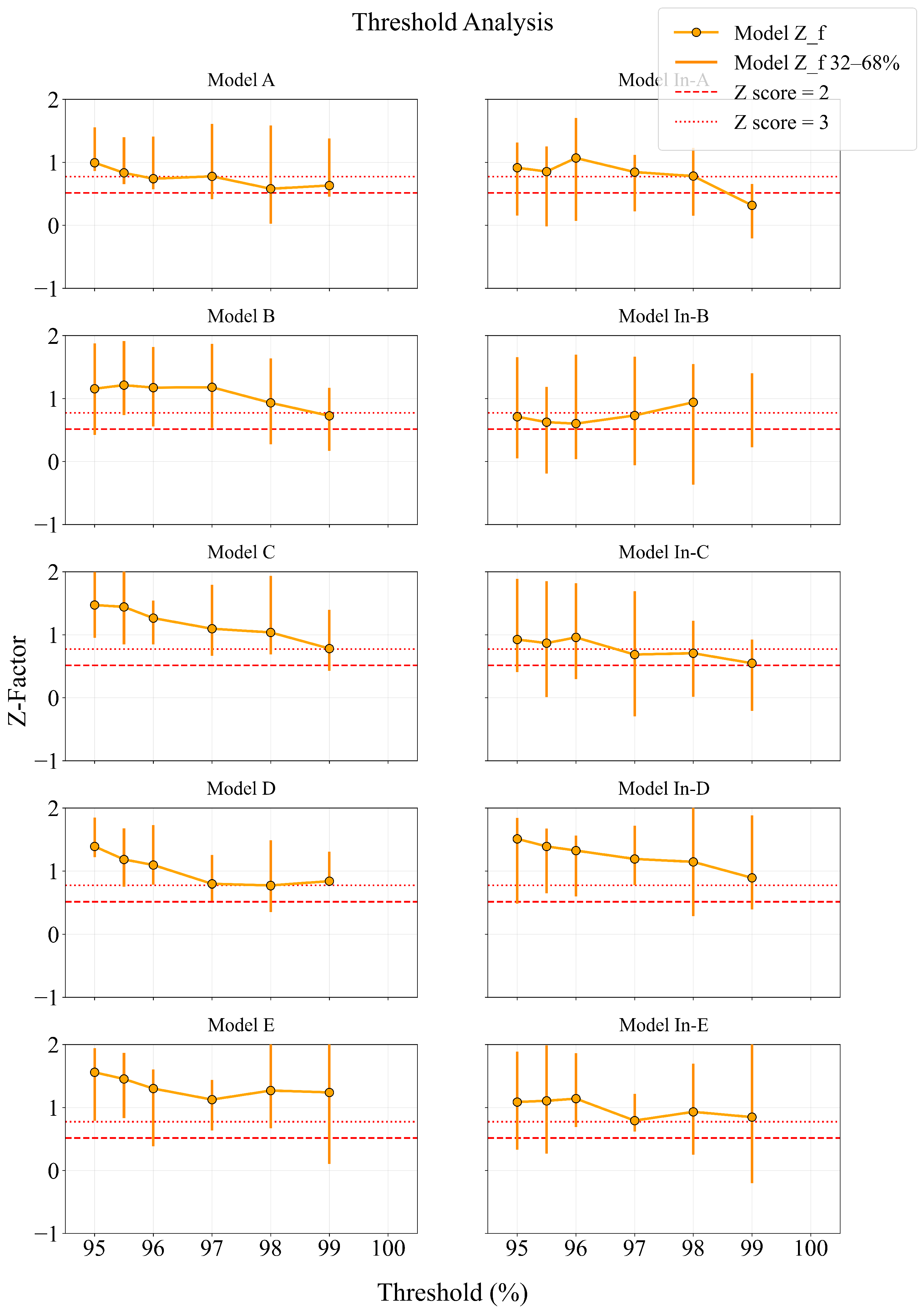
Because the 98th percentile threshold was fixed before any seismic association statistics were computed, the analysis does not benefit from implicit optimisation over different threshold values.
Appendix A.2
We present here the complete set of Z-factor values obtained from all considered spatial (SW) and temporal (TW) window combinations. The window criterion directly affects the classification of sequences into seismic and non-seismic categories, thereby changing the composition of the training dataset and the resulting model behaviour. Each SW-TW configuration therefore corresponds to a distinct modelling scenario rather than a simple parameter tuning step. Table A1 and Table A2 summarise the Z-factor values computed for all configurations for the models trained in the primary phase analysis. The significance threshold used here is ( in this framework), and any value higher than this quantity is written bold in the table.
Table A1.
Z-factor values for each trained model under different spatial window configurations at TW48.
Table A2.
Z-factor values for each trained model under different temporal window configurations at SW22 × 22.
In addition to the absolute value of each score, the number of trained model variants with a Z-factor above this threshold is another sign of robustness. From this point of view, the SW22 × 22_TW48 configuration is unique because it has one of the highest numbers of models, with . This supports the idea that the chosen criterion is not based on just one high-performing model but on a more stable and repeatable pattern across the performance of different models, and thus is selected as the best-performing SW-TW configuration for the study.
References
- Doocy, S.; Daniels, A.; Packer, C.; Dick, A.; Kirsch, T.D. The human impact of earthquakes: A historical review of events 1980–2009 and systematic literature review. PLoS Curr. 2013, 5, 5. [Google Scholar] [CrossRef] [Scilit] [PubMed]
- Aksoy, C.G.; Chupilkin, M.; Koczan, Z.; Plekhanov, A. Unearthing the Economic and Social Consequences of Earthquakes; IZA Discussion Papers No. 17108; Institute of Labor Economics (IZA): Bonn, Germany, 2024. [Google Scholar]
- Udías, A.; Madariaga, R.; Buforn, E. Source Mechanisms of Earthquakes: Theory and Practice; Cambridge University Press: Cambridge, UK, 2014. [Google Scholar]
- Liu, J.Y.; Chen, Y.I.; Jhuang, H.K.; Lin, Y.H. Ionospheric foF2 and TEC Anomalous Days Associated with M > or = 5.0 Earthquakes in Taiwan during 1997–1999. Terr. Atmos. Ocean. Sci. 2004, 15, 371–384. [Google Scholar] [CrossRef] [Scilit]
- Liu, J.Y.; Chen, Y.; Chuo, Y.; Chen, C.S. A statistical investigation of pre-earthquake ionospheric anomaly. J. Geophys. Res. Space Phys. 2006, 111, A05304. [Google Scholar] [CrossRef] [Scilit]
- Kon, S.; Nishihashi, M.; Hattori, K. Ionospheric anomalies possibly associated with M ≥ 6.0 earthquakes in the Japan area during 1998–2010: Case studies and statistical study. J. Asian Earth Sci. 2011, 41, 410–420. [Google Scholar] [CrossRef] [Scilit]
- Ahmed, J.; Shah, M.; Iqbal, T.; Shah, M.A.; Amin, A. Study of the ionospheric precursors associated with Mw ≥ 6.0 EQ from Ionosonde Stations and GIM TEC. J. Atmos. Sol.-Terr. Phys. 2024, 256, 106205. [Google Scholar] [CrossRef] [Scilit]
- Li, M.; Parrot, M. “Real time analysis” of the ion density measured by the satellite DEMETER in relation with the seismic activity. Nat. Hazards Earth Syst. Sci. 2012, 12, 2957–2963. [Google Scholar] [CrossRef] [Scilit]
- Shah, M.; Tariq, M.A.; Ahmad, J.; Naqvi, N.A.; Jin, S. Seismo ionospheric anomalies before the 2007 M7. 7 Chile earthquake from GPS TEC and DEMETER. J. Geodyn. 2019, 127, 42–51. [Google Scholar] [CrossRef] [Scilit]
- Li, Z.; Li, J.; Huang, J.; Yin, H.; Jia, J. Research on pre-seismic feature recognition of spatial electric field data recorded by CSES. Atmosphere 2022, 13, 179. [Google Scholar] [CrossRef] [Scilit]
- Zhu, K.; Li, Z.; Huang, J.; Pan, K.; Hao, B.; Zhang, Y. Ionospheric Schumann Resonance Signal Image Recognition Model and Its Application to the Yangbi Earthquake. Atmosphere 2026, 17, 193. [Google Scholar] [CrossRef] [Scilit]
- Zhang, F.Z.; Huang, J.P.; Li, Z.; Shen, X.H.; Li, W.J.; Wang, Q.; Zeren, Z.; Liu, J.L.; Li, Z.Y.; Chen, Z.Y. Statistical analysis of electric field perturbations in ELF based on the CSES observation data before the earthquake. Front. Earth Sci. 2023, 11, 1101542. [Google Scholar] [CrossRef] [Scilit]
- He, Y.; Zhao, X.; Yang, D.; Wu, Y.; Li, Q. A study to investigate the relationship between ionospheric disturbance and seismic activity based on Swarm satellite data. Phys. Earth Planet. Inter. 2022, 323, 106826. [Google Scholar] [CrossRef] [Scilit]
- Xie, T.; Chen, B.; Wu, L.; Dai, W.; Kuang, C.; Miao, Z. Detecting seismo-ionospheric anomalies possibly associated with the 2019 ridgecrest (California) earthquakes by GNSS, CSES, and Swarm observations. J. Geophys. Res. Space Phys. 2021, 126, e2020JA028761. [Google Scholar] [CrossRef] [Scilit]
- Özsöz, İ.; Pamukçu, O.A. Analysing pre-earthquake magnetic and ionospheric anomalies using swarm satellite data: Findings from the February 6, 2023, Pazarcık, Türkiye earthquake. Adv. Space Res. 2025, 75, 5460–5476. [Google Scholar] [CrossRef] [Scilit]
- Hayakawa, M.; Kasahara, Y.; Nakamura, T.; Muto, F.; Horie, T.; Maekawa, S.; Hobara, Y.; Rozhnoi, A.; Solovieva, M.; Molchanov, O. A statistical study on the correlation between lower ionospheric perturbations as seen by subionospheric VLF/LF propagation and earthquakes. J. Geophys. Res. Space Phys. 2010, 115, A09305. [Google Scholar] [CrossRef] [Scilit]
- Kasahara, Y.; Nakamura, T.; Hobara, Y.; Hayakawa, M.; Rozhnoi, A.; Solovieva, M.; Molchanov, O.A. A statistical study on the AGW modulations in subionospheric VLF/LF propagation data and consideration of the generation mechanism of seismo-ionospheric perturbations. J. Atmos. Electr. 2010, 30, 103–112. [Google Scholar] [CrossRef] [Scilit]
- Eshkuvatov, H.; Ahmedov, B.; Tillayev, Y.; Tariq, M.A.; Shah, M.A.; Liu, L. Ionospheric precursors of strong earthquakes observed using six GNSS stations data during continuous five years (2011–2015). Geod. Geodyn. 2023, 14, 65–79. [Google Scholar] [CrossRef] [Scilit]
- Tachema, A.; Kheloufi, N.; Mohamed, E.K. Investigating Ionospheric Disturbances as Potential Seismic Precursors: A Case Study of the 2021 Béjaïa Mw 6.0 Earthquake, in Northeastern Algeria. J. Indian Soc. Remote Sens. 2025, 53, 847–862. [Google Scholar] [CrossRef] [Scilit]
- Chen, J.; Xiong, P.; Wu, H.; Zhang, X.; Zhang, X.; Zhang, T.; Ruan, Q. Pre-seismic anomalies and co-seismic disturbance induced by the 2024 Mw 7.1 Wushi earthquake: Multi-GNSS observations and modeling. Geomat. Nat. Hazards Risk 2024, 15, 2422024. [Google Scholar] [CrossRef] [Scilit]
- Zulhamidi, N.F.I.; Abdullah, M.; Abdul Hamid, N.S.; Yusof, K.A.; Bahari, S.A. Investigating short-term earthquake precursors detection through monitoring of total electron content variation in ionosphere. Front. Astron. Space Sci. 2023, 10, 1166394. [Google Scholar] [CrossRef] [Scilit]
- Semlali, B.E.B.; Molina, C.; Park, H.; Camps, A. On the correlation between earthquakes and prior ionospheric scintillations over the ocean: A study using GNSS-R data between 2017 and 2021. IEEE J. Sel. Top. Appl. Earth Obs. Remote Sens. 2024, 17, 2640–2654. [Google Scholar] [CrossRef] [Scilit]
- Boudriki Semlali, B.E.; Molina, C.; Park, H.; Camps, A. Ionospheric Scintillation Anomalies from COSMIC-2 GNSS-RO from 2019 and 2024 as Potential Earthquake Precursors. ISPRS Int. J. Geo-Inf. 2026, 15, 128. [Google Scholar] [CrossRef] [Scilit]
- Hameed, A.; Shah, M.; Ghaffar, B.; Riaz, S.; Jamjareegulgarn, P.; Alarifi, N.S.; Abukhadra, M.R. Possible atmospheric-ionospheric precursors of the 2020 Hotan China earthquake from various satellites. Adv. Space Res. 2024, 74, 3326–3343. [Google Scholar] [CrossRef] [Scilit]
- Pulinets, S.; Krankowski, A.; Hernandez-Pajares, M.; Marra, S.; Cherniak, I.; Zakharenkova, I.; Rothkaehl, H.; Kotulak, K.; Davidenko, D.; Blaszkiewicz, L.; et al. Ionosphere Sounding for Pre-seismic anomalies identification (INSPIRE): Results of the project and Perspectives for the short-term earthquake forecast. Front. Earth Sci. 2021, 9, 610193. [Google Scholar] [CrossRef] [Scilit]
- Hayakawa, M.; Solovieva, M.; Kopylova, G.; Hirooka, S.; Sasmal, S.; Nanda, K.; Yang, S.S.; Michimoto, K.; Hinata, H. Multi-Parameter and Multi-Layer Observations of Electromagnetic Precursors to a Huge Hokkaido Earthquake (M = 6.7) on 5 September, 2018, and Lithosphere–Atmosphere–Ionosphere Coupling Channel. Atmosphere 2025, 16, 1372. [Google Scholar] [CrossRef] [Scilit]
- Hayakawa, M. Seismo Electromagnetics: Lithosphere-Atmosphere-Ionosphere Coupling; Terrapub: Tokyo, Japan, 2002. [Google Scholar]
- Pulinets, S.; Boyarchuk, K. Ionospheric Precursors of Earthquakes; Springer: Berlin/Heidelberg, Germany, 2004. [Google Scholar]
- Varotsos, P.; Alexopoulos, K.; Nomicos, K.; Lazaridou, M. Earthquake prediction and electric signals. Nature 1986, 322, 120. [Google Scholar] [CrossRef] [Scilit]
- Varotsos, P.A. The Physics of Seismic Electric Signals; Terrapub: Tokyo, Japan, 2005. [Google Scholar]
- Hattori, K. ULF geomagnetic changes associated with major earthquakes. In Earthquake Prediction Studies: Seismo Electromagnetics; TERRAPUB: Tokyo, Japan, 2013; pp. 129–152. [Google Scholar]
- Akhoondzadeh, M. Novelty detection in time series of ULF magnetic and electric components obtained from DEMETER satellite experiments above Samoa (29 September 2009) earthquake region. Nat. Hazards Earth Syst. Sci. 2013, 13, 15–25. [Google Scholar] [CrossRef] [Scilit]
- Eftaxias, K.; Potirakis, S. Current challenges for pre-earthquake electromagnetic emissions: Shedding light from micro-scale plastic flow, granular packings, phase transitions and self-affinity notion of fracture process. Nonlinear Process. Geophys. 2013, 20, 771–792. [Google Scholar] [CrossRef] [Scilit]
- Potirakis, S.M.; Contoyiannis, Y.; Melis, N.S.; Kopanas, J.; Antonopoulos, G.; Balasis, G.; Kontoes, C.; Nomicos, C.; Eftaxias, K. Recent seismic activity at Cephalonia (Greece): A study through candidate electromagnetic precursors in terms of non-linear dynamics. Nonlinear Process. Geophys. 2016, 23, 223–240. [Google Scholar] [CrossRef] [Scilit]
- Potirakis, S.; Contoyiannis, Y.; Schekotov, A.; Eftaxias, K.; Hayakawa, M. Evidence of critical dynamics in various electromagnetic precursors. Eur. Phys. J. Spec. Top. 2021, 230, 151–177. [Google Scholar] [CrossRef] [Scilit]
- Eftaxias, K.; Potirakis, S.M.; Contoyiannis, Y. Four-stage model of earthquake generation in terms of fracture-induced electromagnetic emissions: A review. In Complexity of Seismic Time Series: Measurement and Application, 1st ed.; Elsevier: Amsterdam, The Netherlands, 2018; pp. 437–502. [Google Scholar]
- Parrot, M. The micro-satellite DEMETER. J. Geodyn. 2002, 33, 535–541. [Google Scholar] [CrossRef] [Scilit]
- Korepanov, V.; Hayakawa, M.; Yampolski, Y.; Lizunov, G. AGW as a seismo-ionospheric coupling responsible agent. Phys. Chem. Earth Parts A/B/C 2009, 34, 485–495. [Google Scholar] [CrossRef] [Scilit]
- Piersanti, M.; Materassi, M.; Battiston, R.; Carbone, V.; Cicone, A.; D’Angelo, G.; Diego, P.; Ubertini, P. Magnetospheric–ionospheric–lithospheric coupling model. 1: Observations during the 5 August 2018 Bayan Earthquake. Remote Sens. 2020, 12, 3299. [Google Scholar] [CrossRef] [Scilit]
- Freund, F. Toward a unified solid state theory for pre-earthquake signals. Acta Geophys. 2010, 58, 719–766. [Google Scholar] [CrossRef] [Scilit]
- Pulinets, S.; Ouzounov, D. Lithosphere–Atmosphere–Ionosphere Coupling (LAIC) model–An unified concept for earthquake precursors validation. J. Asian Earth Sci. 2011, 41, 371–382. [Google Scholar] [CrossRef] [Scilit]
- Molchanov, O.; Hayakawa, M. On the generation mechanism of ULF seismogenic electromagnetic emissions. Phys. Earth Planet. Inter. 1998, 105, 201–210. [Google Scholar] [CrossRef] [Scilit]
- Kopytenko, Y.; Ismagilov, V.; Hayakawa, M.; Smirnova, N.; Troyan, V.; Peterson, T. Investigation of the ULF electromagnetic phenomena related to earthquakes. Contemporary achievements and the perspectives. Ann. Geophys. 2001, 44, 325–334. [Google Scholar]
- Carbone, V.; Piersanti, M.; Materassi, M.; Battiston, R.; Lepreti, F.; Ubertini, P. A mathematical model of lithosphere-atmosphere coupling for seismic events. Sci. Rep. 2021, 11, 8682. [Google Scholar] [CrossRef] [Scilit]
- Galkina, A.; Grafeeva, N. Machine learning methods for earthquake prediction: A survey. In Proceedings of the Fourth Conference on Software Engineering and Information Management (SEIM-2019), Saint Petersburg, Russia, 13 April 2019; Volume 13, p. 25. [Google Scholar]
- Asaly, S.; Gottlieb, L.A.; Inbar, N.; Reuveni, Y. Using support vector machine (SVM) with GPS ionospheric TEC estimations to potentially predict earthquake events. Remote Sens. 2022, 14, 2822. [Google Scholar] [CrossRef] [Scilit]
- Akyol, A.A.; Arikan, O.; Arikan, F. A machine learning-based detection of earthquake precursors using ionospheric data. Radio Sci. 2020, 55, e2019RS006931. [Google Scholar] [CrossRef] [Scilit]
- Tsai, T.; Jhuang, H.; Ho, Y.; Lee, L.; Su, W.; Hung, S.; Lee, K.; Fu, C.; Lin, H.; Kuo, C. Deep learning of detecting ionospheric precursors associated with M ≥ 6.0 earthquakes in Taiwan. Earth Space Sci. 2022, 9, e2022EA002289. [Google Scholar] [CrossRef] [Scilit]
- Uyanık, H.; Şentürk, E.; Akpınar, M.H.; Ozcelik, S.T.; Kokum, M.; Freeshah, M.; Sengur, A. A multi-input convolutional neural networks model for earthquake precursor detection based on ionospheric total electron content. Remote Sens. 2023, 15, 5690. [Google Scholar] [CrossRef] [Scilit]
- Xiong, P.; Long, C.; Zhou, H.; Battiston, R.; Zhang, X.; Shen, X. Identification of electromagnetic pre-earthquake perturbations from the DEMETER data by machine learning. Remote Sens. 2020, 12, 3643. [Google Scholar] [CrossRef] [Scilit]
- Akhoondzadeh, M.; De Santis, A.; Marchetti, D.; Wang, T. Developing a Deep Learning-Based Detector of Magnetic, Ne, Te and TEC Anomalies from Swarm Satellites: The Case of Mw 7.1 2021 Japan Earthquake. Remote Sens. 2022, 14, 1582. [Google Scholar] [CrossRef] [Scilit]
- Ravanelli, M.; Constantinou, V.; Liu, H.; Bortnik, J. Exploring AI progress in GNSS remote sensing: A deep learning based framework for real-time detection of earthquake and tsunami induced ionospheric perturbations. Radio Sci. 2024, 59, e2024RS008016. [Google Scholar] [CrossRef] [Scilit]
- Draz, M.U.; Shah, M.; Jamjareegulgarn, P.; Shahzad, R.; Hasan, A.M.; Ghamry, N.A. Deep machine learning based possible atmospheric and ionospheric precursors of the 2021 Mw 7.1 Japan earthquake. Remote Sens. 2023, 15, 1904. [Google Scholar] [CrossRef] [Scilit]
- Zhang, R.; Li, H.; Shen, Y.; Yang, J.; Li, W.; Zhao, D.; Hu, A. Deep learning applications in ionospheric modeling: Progress, challenges, and opportunities. Remote Sens. 2025, 17, 124. [Google Scholar] [CrossRef] [Scilit]
- Berthelier, J.J.; Godefroy, M.; Leblanc, F.; Malingre, M.; Menvielle, M.; Lagoutte, D.; Brochot, J.; Colin, F.; Elie, F.; Legendre, C.; et al. ICE, the electric field experiment on DEMETER. Planet. Space Sci. 2006, 54, 456–471. [Google Scholar] [CrossRef] [Scilit]
- Mueller, C.S. Earthquake catalogs for the USGS national seismic hazard maps. Seismol. Res. Lett. 2019, 90, 251–261. [Google Scholar] [CrossRef] [Scilit]
- Chen, H.; Han, P.; Hattori, K. Recent advances and challenges in the seismo-electromagnetic study: A brief review. Remote Sens. 2022, 14, 5893. [Google Scholar] [CrossRef] [Scilit]
- Hochreiter, S.; Schmidhuber, J. Long short-term memory. Neural Comput. 1997, 9, 1735–1780. [Google Scholar] [CrossRef] [Scilit]
- Michelucci, U. An introduction to autoencoders. arXiv 2022, arXiv:2201.03898. [Google Scholar] [CrossRef] [Scilit]
- Nguyen, H.D.; Tran, K.P.; Thomassey, S.; Hamad, M. Forecasting and Anomaly Detection approaches using LSTM and LSTM Autoencoder techniques with the applications in supply chain management. Int. J. Inf. Manag. 2021, 57, 102282. [Google Scholar] [CrossRef] [Scilit]
- Chen, Z.; Yeo, C.K.; Lee, B.S.; Lau, C.T. Autoencoder-based network anomaly detection. In Proceedings of the 2018 Wireless Telecommunications Symposium (WTS); IEEE: New York, NY, USA, 2018; pp. 1–5. [Google Scholar]
- Malhotra, P. LSTM-based Encoder-Decoder for Multi-sensor Anomaly Detection. arXiv 2016, arXiv:1607.00148. [Google Scholar]
- Provotar, O.I.; Linder, Y.M.; Veres, M.M. Unsupervised anomaly detection in time series using lstm-based autoencoders. In Proceedings of the 2019 IEEE International Conference on Advanced Trends in Information Theory (ATIT); IEEE: New York, NY, USA, 2019; pp. 513–517. [Google Scholar]
- Pereira, J.; Silveira, M. Unsupervised anomaly detection in energy time series data using variational recurrent autoencoders with attention. In Proceedings of the 2018 17th IEEE International Conference on Machine Learning and Applications (ICMLA); IEEE: New York, NY, USA, 2018; pp. 1275–1282. [Google Scholar]
- Principi, E.; Rossetti, D.; Squartini, S.; Piazza, F. Unsupervised electric motor fault detection by using deep autoencoders. IEEE/CAA J. Autom. Sin. 2019, 6, 441–451. [Google Scholar] [CrossRef] [Scilit]
- Pandey, R.; Khatri, S.K.; Singh, N.K.; Verma, P. Artificial Intelligence and Machine Learning for EDGE Computing; Academic Press: Cambridge, MA, USA, 2022. [Google Scholar]
- Kinga, D.; Adam, J.B. A method for stochastic optimization. arXiv 2014, arXiv:1412.6980. [Google Scholar] [CrossRef] [Scilit]
- Raximov, N.; Kuvandikov, J.; Dilmurod, K. The importance of loss function in artificial intelligence. In Proceedings of the 2022 International Conference on Information Science and Communications Technologies (ICISCT); IEEE: New York, NY, USA, 2022; pp. 1–3. [Google Scholar]
- Stouffer, S.A.; Suchman, E.A.; DeVinney, L.C.; Star, S.A.; Williams, R.M., Jr. The American Soldier, Vol. 1: Adjustment During Army Life; Princeton University Press: Princeton, NJ, USA, 1949; p. 45. [Google Scholar]
- Whitlock, M.C. Combining probability from independent tests: The weighted Z-method is superior to Fisher’s approach. J. Evol. Biol. 2005, 18, 1368–1373. [Google Scholar] [CrossRef] [Scilit]
- Clette, F.; Svalgaard, L.; Vaquero, J.M.; Cliver, E.W. Revisiting the sunspot number: A 400-year perspective on the solar cycle. Space Sci. Rev. 2014, 186, 35–103. [Google Scholar] [CrossRef] [Scilit]
- Li, Z.; Tao, Z.; Cao, L. Analysis of Ionospheric Anomalies before Earthquakes of Mw6.5 and above in Japan from 2011 to 2022. Atmosphere 2024, 15, 887. [Google Scholar] [CrossRef] [Scilit]
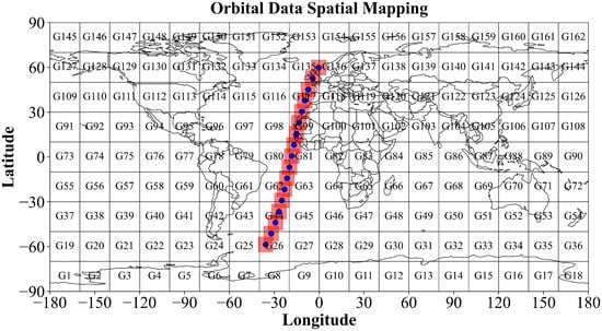
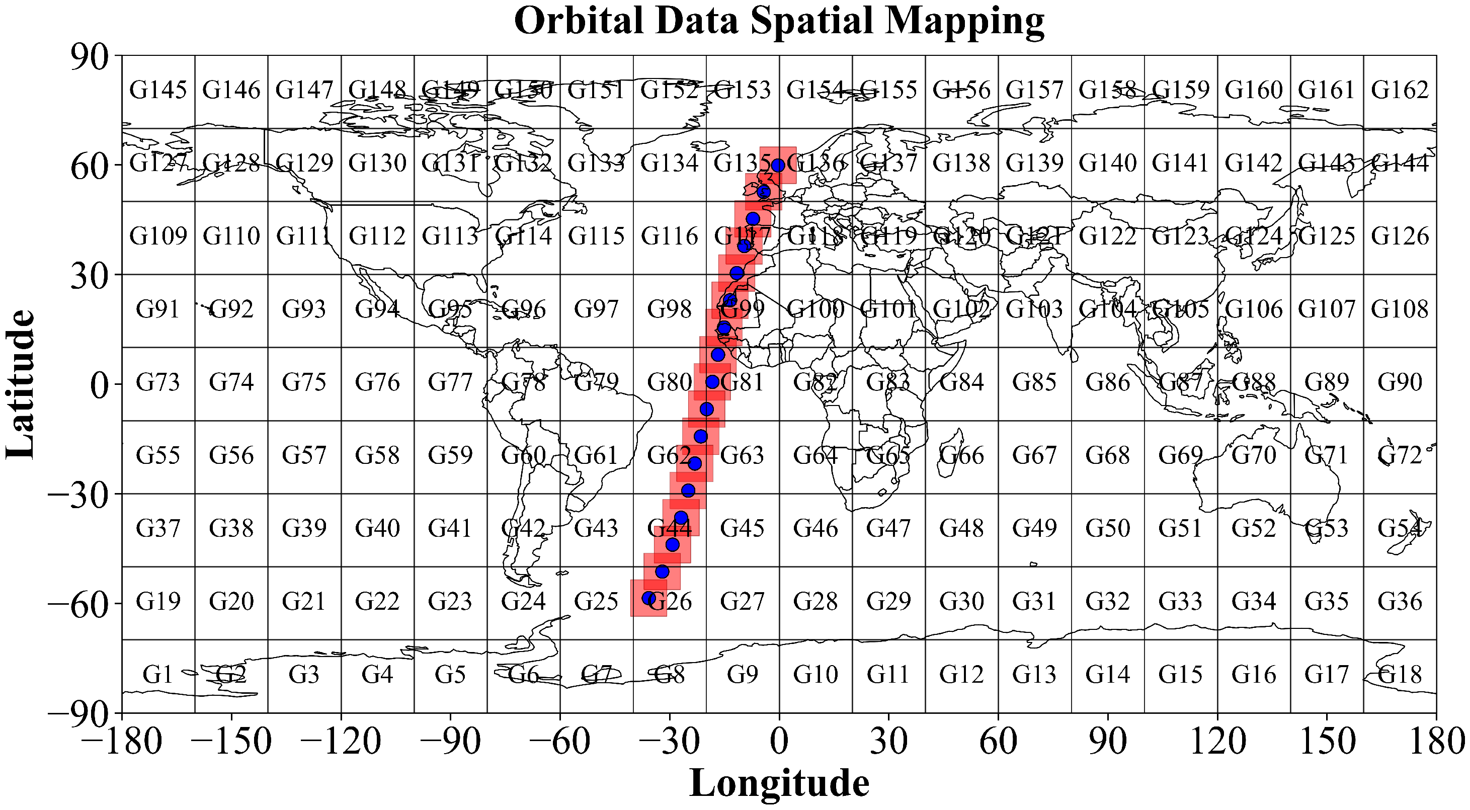
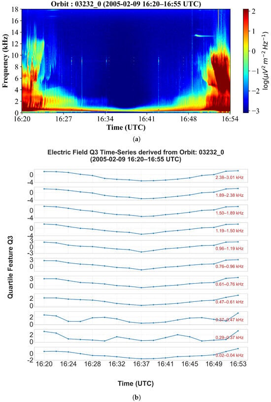
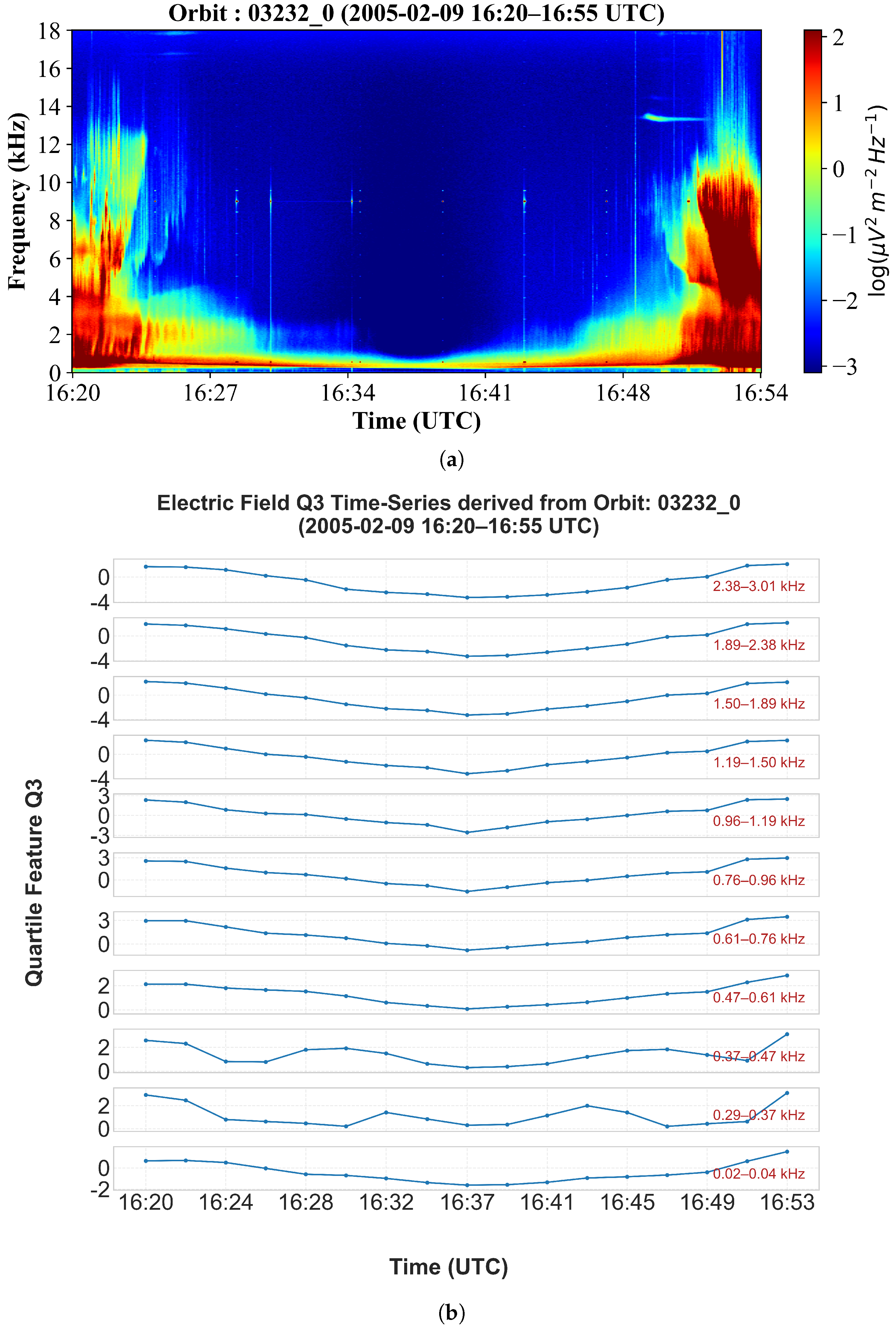
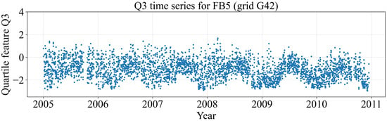
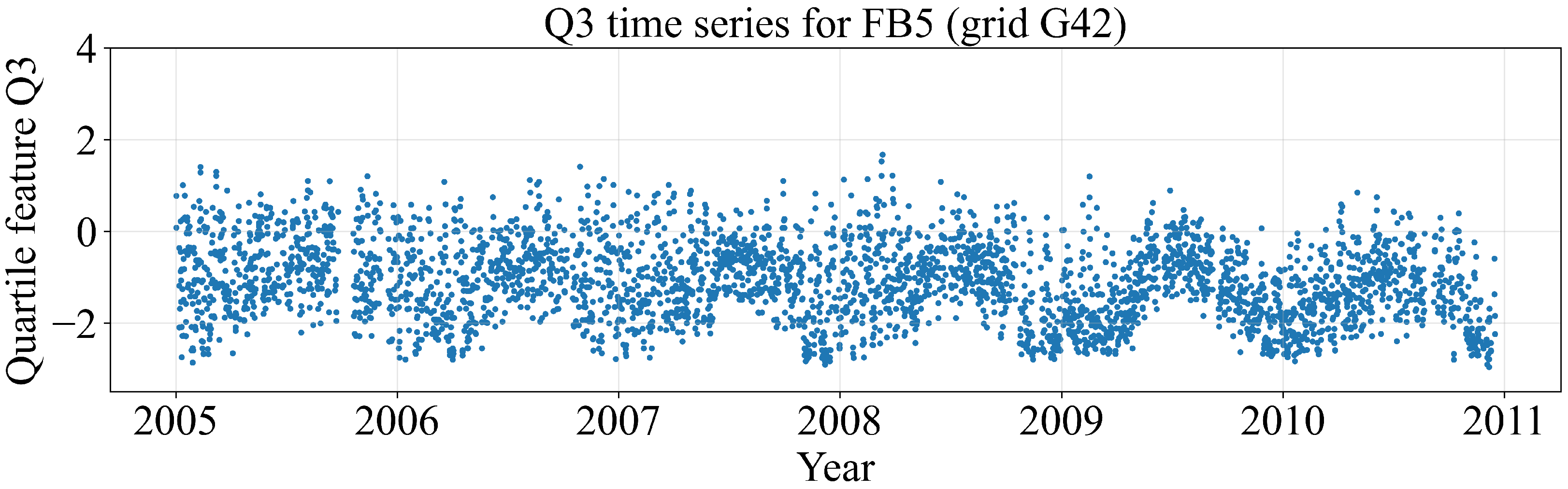
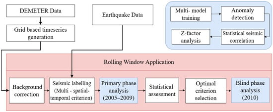
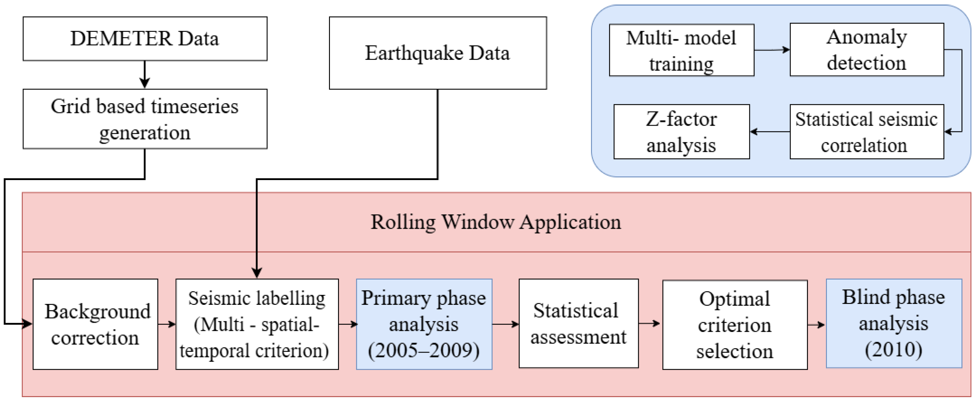
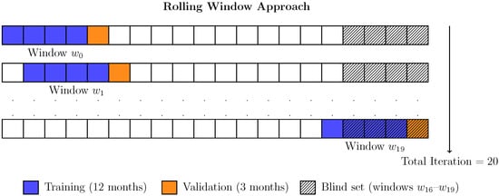
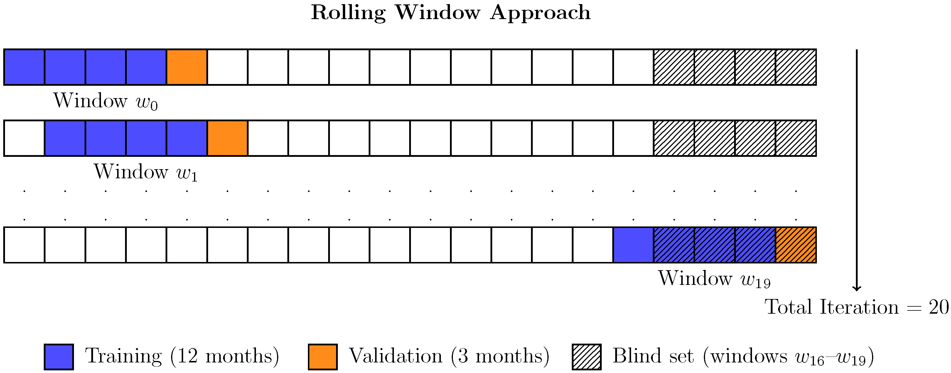
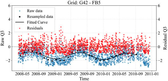
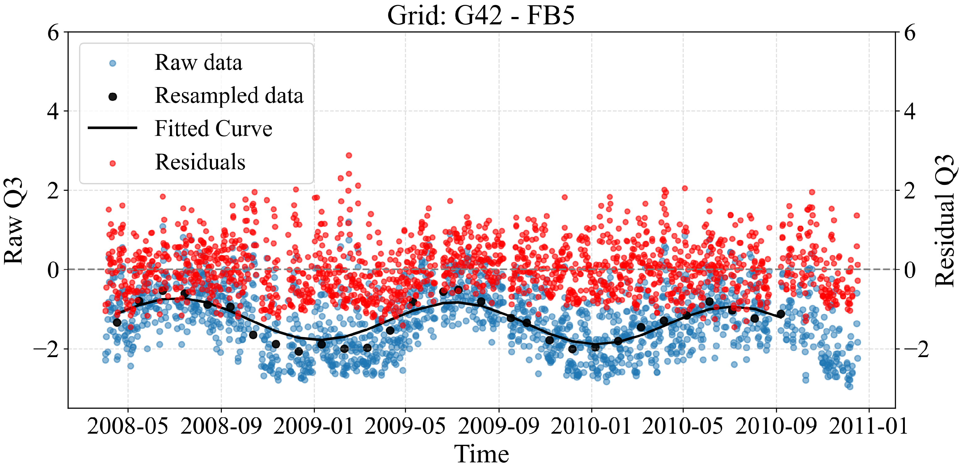
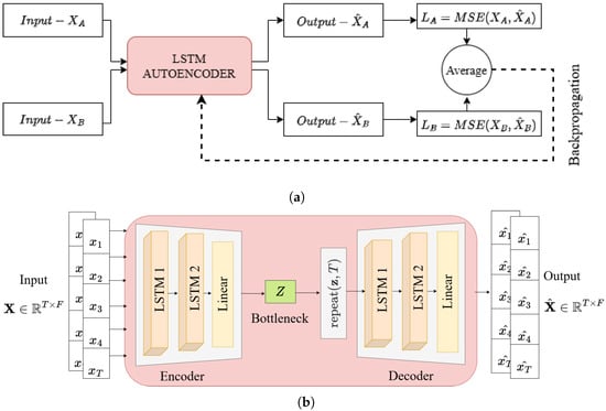
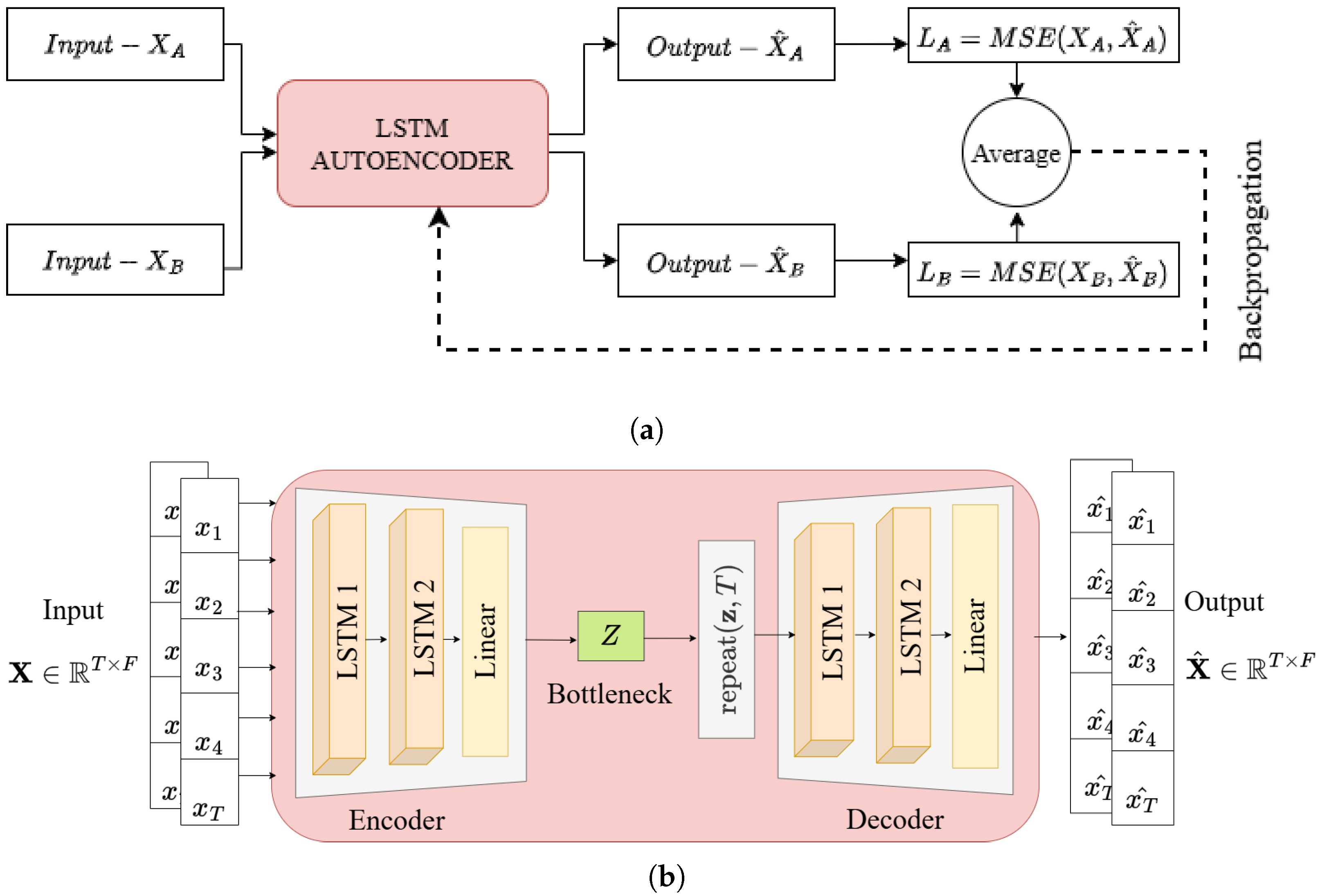
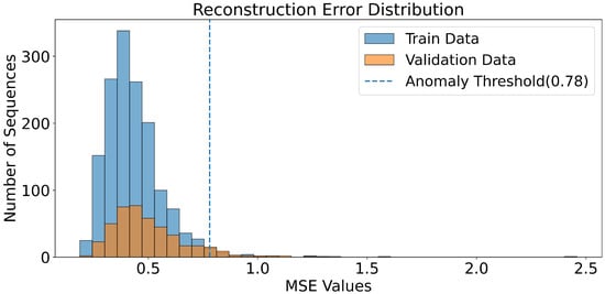
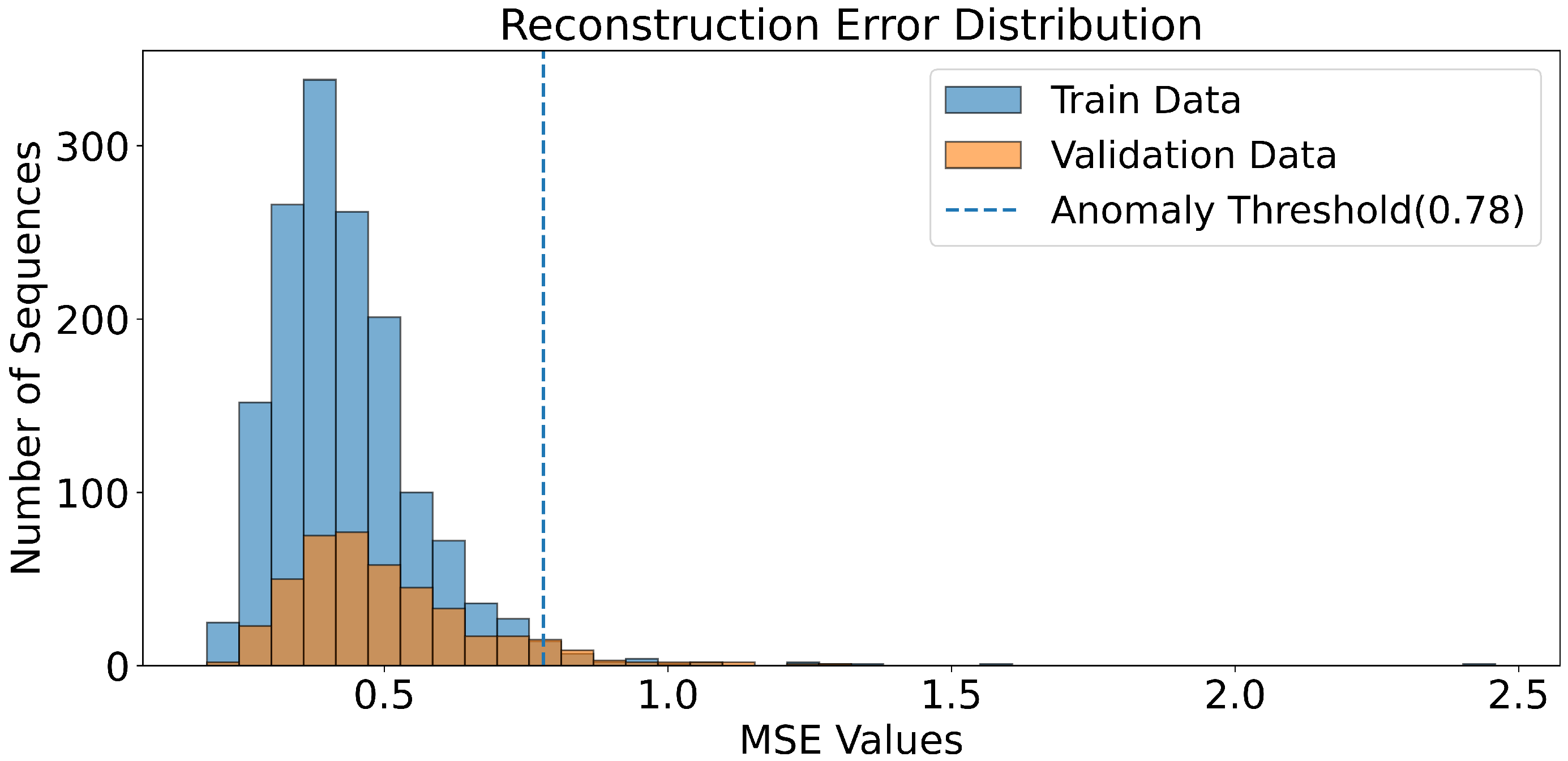
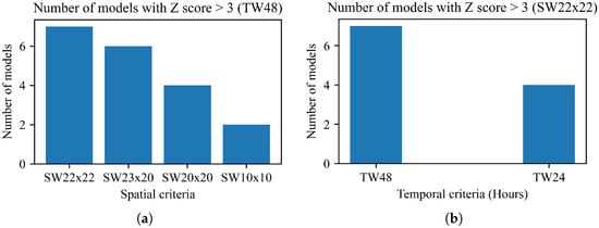
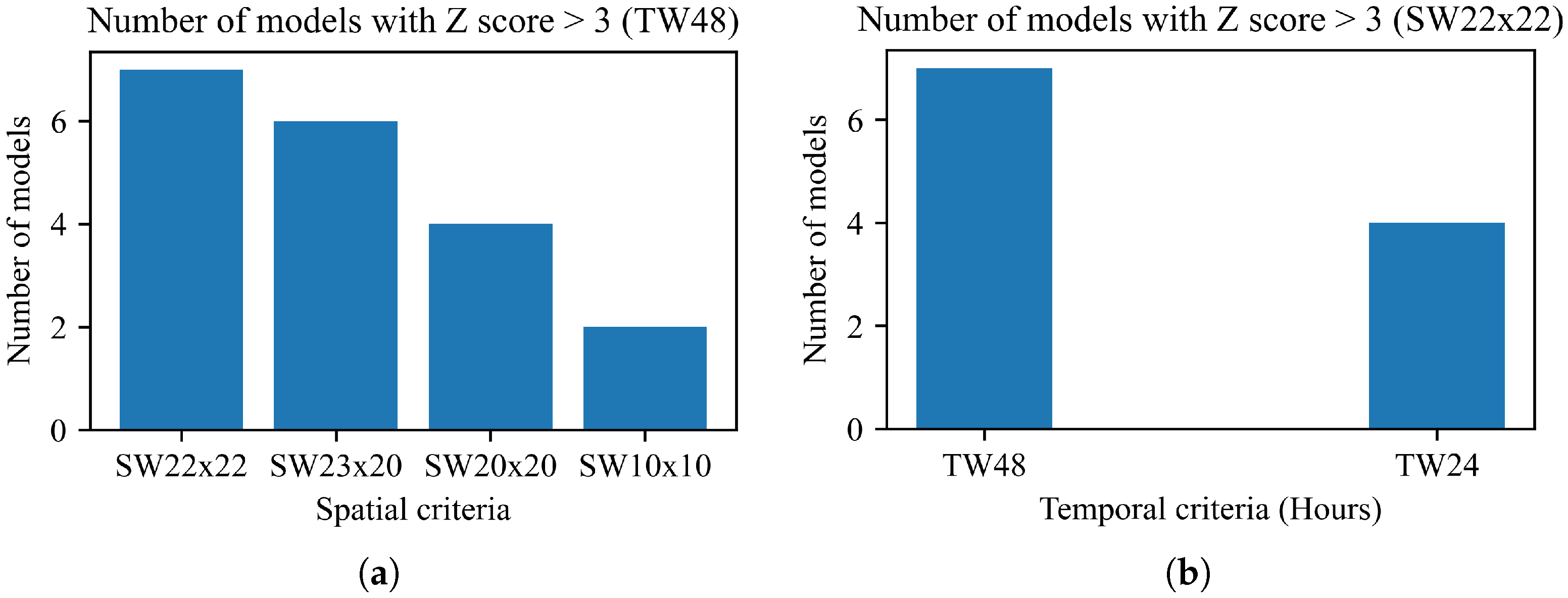
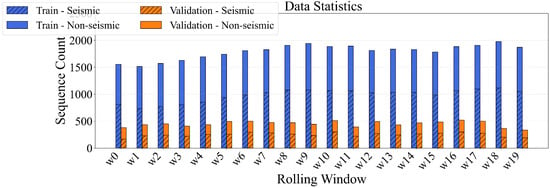
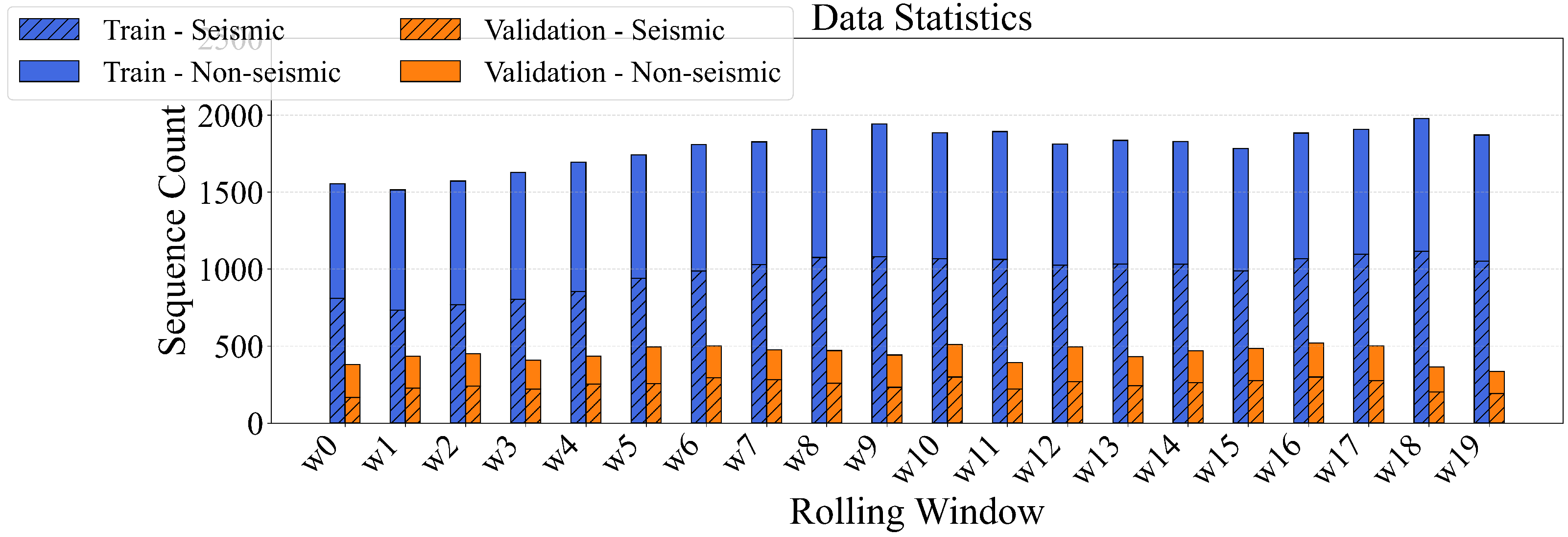
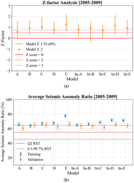
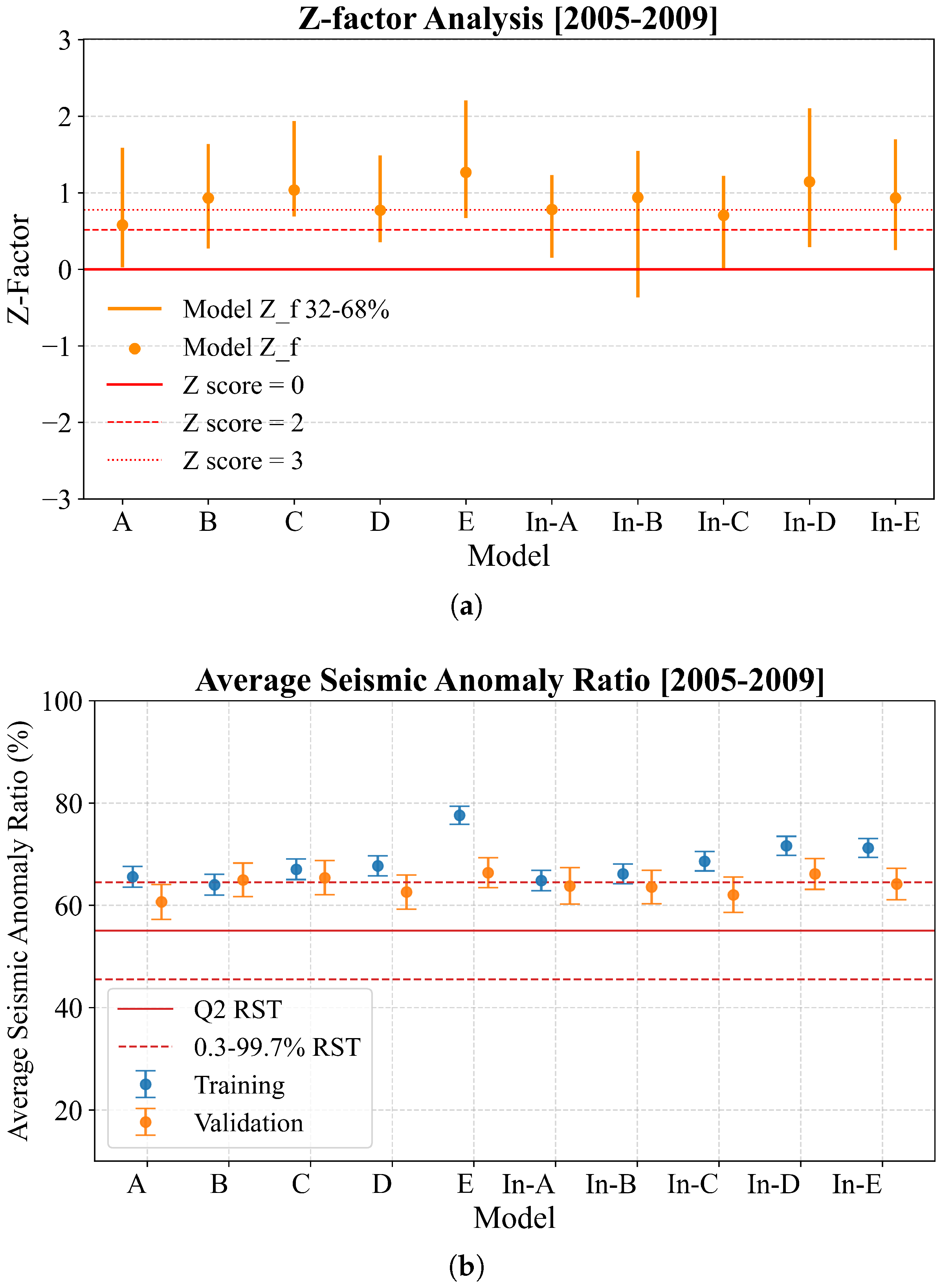
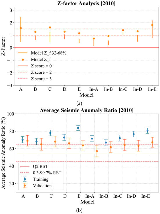
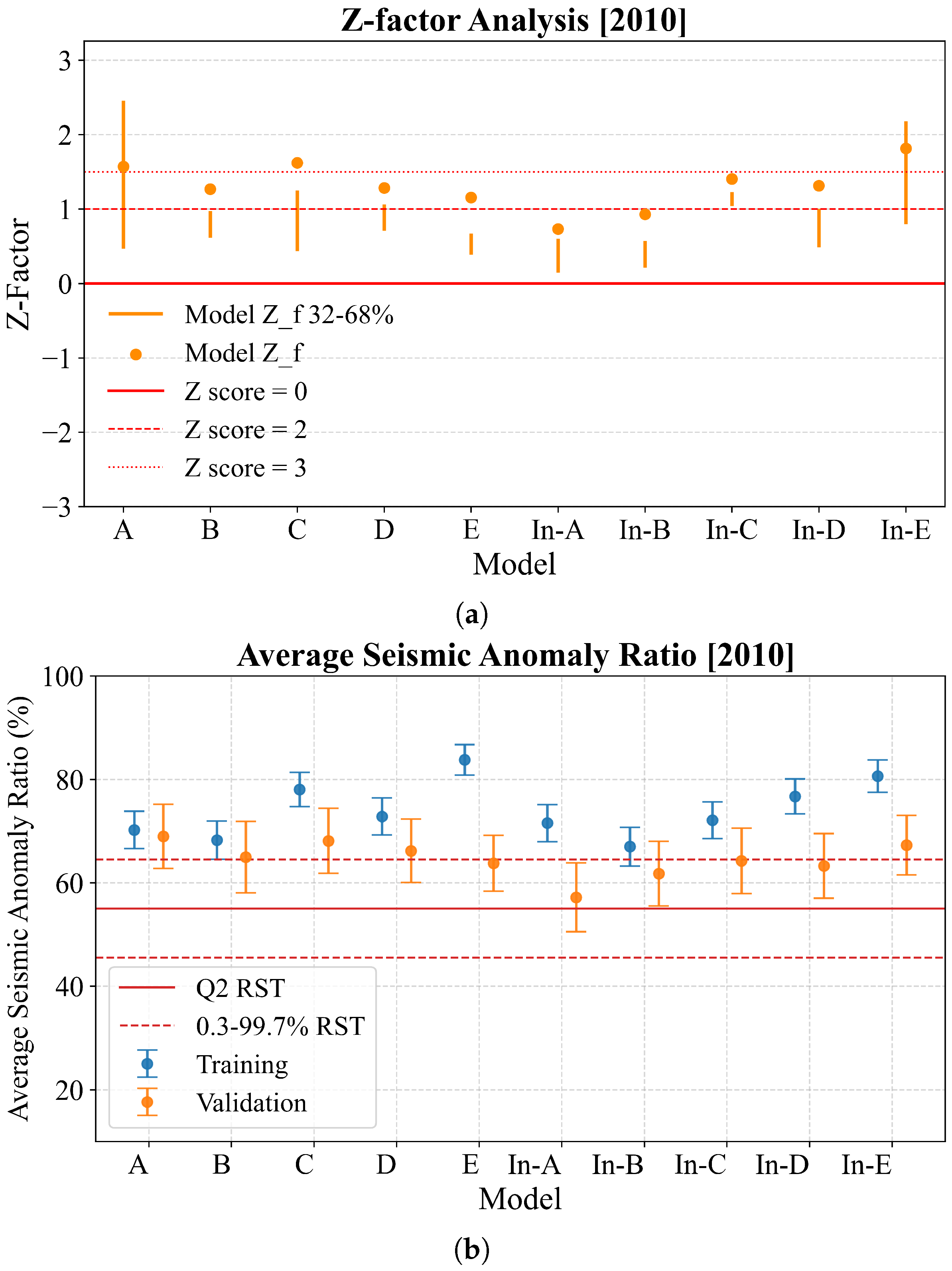
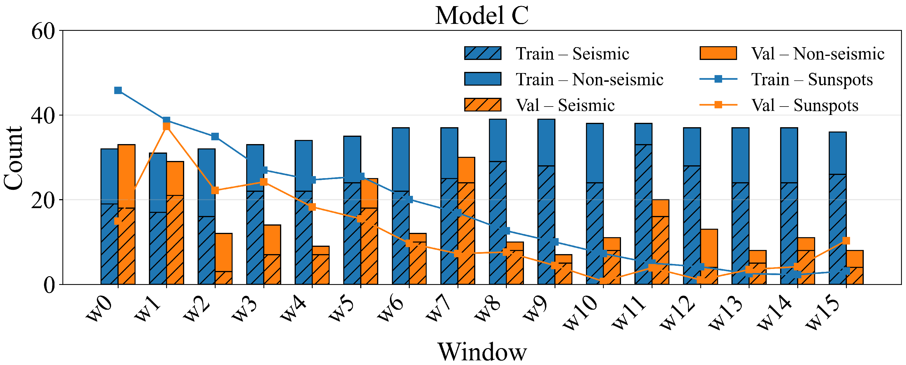

Disclaimer/Publisher’s Note: The statements, opinions and data contained in all publications are solely those of the individual author(s) and contributor(s) and not of MDPI and/or the editor(s). MDPI and/or the editor(s) disclaim responsibility for any injury to people or property resulting from any ideas, methods, instructions or products referred to in the content. |
© 2026 by the authors. Licensee MDPI, Basel, Switzerland. This article is an open access article distributed under the terms and conditions of the Creative Commons Attribution (CC BY) license.