


Highlights
What are the main findings?
- A novel dual-branch network (TCSNet) uses a PVTv2-B2 Transformer to capture long-range spectral dependencies and a CNN to extract multi-scale local spatial features. This combination improves thin-cloud detection in hyperspectral imagery.
- The proposed Cross-Modal Fusion (CMF) module uses a lightweight single-channel gate to integrate spectral-spatial features. The Combined Attention Mechanism (CAM) at the decoder stage enhances sensitivity to thin clouds by focusing on important channels, salient regions, and cloud boundaries.
What are the implications of the main findings?
- By achieving a thin-cloud recall of 85.59% on Gaofen-5 hyperspectral data—substantially outperforming existing methods—TCSNet provides a more reliable solution for quantitative remote sensing applications, which are often compromised by thin-cloud contamination.
- The proposed SS-PCA dimensionality reduction strategy reduces data while preserving thin-cloud-sensitive spectral information, overcoming the limitation of traditional dimensionality reduction methods that weaken the inherent advantages of hyperspectral data. This offers a new approach for dimensionality reduction in hyperspectral imagery.
Abstract
Cloud detection is essential for quantitative land-surface remote sensing and cloud-climate research. However, existing methods often prioritize spatial features over spectral features, which limits thin-cloud detection. To address this issue, this paper proposes a Thin-Cloud-Sensitive Network (TCSNet) for hyperspectral imagery. TCSNet employs an encoder–decoder architecture with a dual-branch design: a convolutional neural network (CNN) extracts multi-scale local features, while a PVTv2-B2 Transformer captures long-range spectral dependencies. To effectively integrate the complementary representations from both branches, a Cross-Modal Fusion (CMF) module with a lightweight single-channel gate is introduced at each stage, followed by a channel attention mechanism (SE) for feature recalibration. Subsequently, a Multi-Scale Fusion (MSF) module is used to integrate multi-level features through a top-down pathway, enabling deep semantic information to guide shallow feature expression. Furthermore, to enhance the decoder’s feature representation capability, a Combined Attention Mechanism (CAM) is incorporated at each decoder stage. This design enables the network to simultaneously focus on important channels, salient regions, and cloud boundaries, effectively alleviating spectral confusion between thin clouds and the underlying surface. Experimental results on Gaofen-5 01 hyperspectral data demonstrate that TCSNet achieves the highest recall (92.98%), (85.59%), and (99.75%), thereby validating its superiority for thin-cloud detection.
1. Introduction
With the rapid advancement of hyperspectral remote sensing technology, hyperspectral satellite images have been widely used for environmental monitoring [1,2], resource survey [3], and urban development assessment [4]. This technology provides irreplaceable technical support for large-scale, high-precision quantitative remote sensing. However, the effectiveness of optical remote sensing is severely compromised by frequent cloud cover, which fundamentally limits its application reliability. According to the report of the International Satellite Cloud Climatology Project (ISCCP), approximately 65% of the Earth’s surface is covered by clouds annually [5]. Thick clouds obscure surface information, leading to data loss [6], while thin clouds cause spectral distortion and spatial texture blurring, affecting the accuracy of quantitative inversion of surface parameters such as land classification and change detection [7], ocean parameter retrieval [8], and aerosol and near-surface particulate matter inversion [9]. Consequently, accurate cloud detection is fundamental to remote sensing data quality control, enabling valid observation screening, ensuring reliable surface parameter inversion, and serving as a basis for cloud-climate studies.
Since the 1980s, a large number of cloud detection methods have been proposed, which can be grouped into three distinct categories: traditional threshold-based methods, machine learning-based methods, and deep learning-based methods. Traditional threshold-based cloud detection methods rely on spectral reflectance differences between clouds and underlying surfaces in specific bands (e.g., the shortwave infrared 1.38 μm band), using manually set discrimination rules to identify and segment cloud pixels. As traditional yet efficient cloud identification algorithms, these methods have been widely applied in official image quality assessments for various satellites, such as ACCA [5] and Fmask [7] for the Landsat series, Sen2Cor [10] for Sentinel-2, and CloudMask [11] for MODIS. In recent years, novel threshold-based approaches have emerged, incorporating multi-temporal information [12,13], dynamic thresholds [14,15], and spectral feature matching tailored for hyperspectral imagery [16]. These methods are straightforward to implement and conceptually clear, typically requiring remote sensing images with relatively abundant spectral information. However, due to the narrow band intervals in hyperspectral images, they are more susceptible to noise when dealing with thin clouds, leading to false positives and missed detections [16]. Moreover, their performance heavily relies on manually set thresholds, resulting in limited generalization capability and a tendency for misdetection in complex scenarios (e.g., thin-cloud coverage or high-reflectance surfaces). For instance, the Fmask [7] algorithm exhibits false positive rates of 15–30% over highly reflective surfaces (e.g., snow-covered areas, deserts) and in scenes containing thin clouds. Finally, threshold rules are often designed for specific sensors and are influenced by variations in surface and atmospheric conditions as well as differences in spectral response functions across sensors, making it challenging to develop a unified, robust model applicable across diverse geographical regions, temporal scales, and sensor types.
To address the limitations of traditional threshold-based cloud detection methods—such as excessive reliance on manually set thresholds, insufficient scene adaptability, and poor robustness—classical machine learning approaches have been introduced to the field of cloud detection. Researchers utilize labeled training data and employ meticulously designed spectral, textural, and local statistical features, as well as combinations thereof, to achieve cloud pixel identification and segmentation through models including classical Bayesian classifiers [17], fuzzy clustering [18], artificial neural networks (ANN) [19], support vector machines (SVM) [20,21], and random forests (RF) [22,23]. The SVM-based cloud detection algorithm STmask [21] generates multi-category masks (e.g., cloud, water, shadow) on Landsat datasets, achieving superior cloud detection accuracy compared to the official Landsat algorithm CFmask. In contrast to traditional threshold-based methods, classical machine learning-based cloud detection methods eliminate the need for manual threshold setting. However, the performance of these methods remains highly dependent on domain knowledge for feature selection, and the manual feature design process is inefficient, often requiring extensive computation to achieve acceptable detection accuracy. Furthermore, when confronted with complex ground-object scenarios, the classification accuracy of classical machine learning-based cloud detection methods may decline significantly. For example, the RF-based cloud detection method RFmask [23] demonstrates improved identification of broken and thin clouds in Landsat imagery and effectively distinguishes most cloud layers from bright underlying surfaces. Nevertheless, its capability to separate clouds from snow and ice in mixed cloud–snow scenarios remains notably inadequate.
In recent years, deep learning-based cloud detection methods, particularly those employing convolutional neural networks (CNNs), have significantly enhanced adaptability to complex cloud formations and variable environmental conditions by leveraging their capacity for automatic extraction of spatial and semantic features. Owing to their high detection accuracy and strong generalization performance, these methods have effectively overcome the limitations of traditional approaches and have become a research focus in the field of cloud detection. Semantic segmentation models originally developed for natural images, such as FCN [24], U-Net [25], and DeeplabV3+ [26], have been adapted for cloud detection. Furthermore, researchers have developed various cloud detection methods tailored to the specific characteristics and challenges of the task, including ECDNet [27] and MF-CNN [28] for Landsat imagery, GCDB-Unet [29] and LGCNet [30] for MODIS imagery, CD-FM3SF [31] and KappaMask [32] for Sentinel-2 imagery, as well as DABNet [33] and GeoInfoNet [34] for GaoFen series satellites. Most current methods primarily focus on the overall spatial-scale characteristics of clouds, without fully accounting for feature variations among different cloud regions caused by differences in cloud thickness. While existing methods perform excellently in conventional cloud detection tasks, they still exhibit deficiencies in the accurate identification of thin clouds. The MF-CNN [28] model demonstrates limitations in extracting deep features of thin clouds, with its thin-cloud recall (76.93%) and detection accuracy (78.13%) significantly lower than the corresponding metrics for thick-cloud detection (89.46% and 90.74%). Li et al. [31] observed that due to the limited number of thin-cloud samples in experimental datasets, the CD-FM3SF model’s ability to accurately detect thin clouds is markedly inferior to its performance on thick clouds. Xu et al. [35] noted that the small size, sparse distribution, and high transparency of thin clouds make them resemble non-cloud background regions, leading existing methods to easily overlook thin clouds.
To enhance the capability of deep learning-based cloud detection methods in identifying thin clouds, researchers have implemented various optimizations to CNN architectures, specifically targeting the representational characteristics of thin clouds in remote sensing imagery. Xu et al. [35] proposed the Thin-Cloud-Aware Network (TANet), which strengthens thin-cloud feature learning across multiple dimensions—such as color, texture, and spatial distribution—through color prior guidance and global information aggregation modules. However, this method exhibits a high missed-detection rate when processing scattered thin clouds, indicating that its perception capability for sparse thin clouds requires further improvement. Li et al. [36] introduced the Pyramid Context Network (PCNet), which expands the receptive field by incorporating dilated residual blocks to overcome the limitations of traditional convolutional kernels, and employs pyramid context blocks to enhance multi-scale feature perception. This approach achieved a recall rate of 93.2% and an overall accuracy of 97.1% on FY-3D MERSI-II RGB imagery. Shi et al. [37] developed a deep learning-based cloud detection method that enhances the expressive capacity for deep features of cloud layers. It demonstrates excellent performance in detecting both thin and thick clouds, as well as strong adaptability to complex scenarios, particularly showing high accuracy in cloud boundary identification.
The introduction of attention mechanisms and Transformer architectures has significantly enhanced the performance of cloud detection models. By simulating the allocation of attention in human cognition, attention mechanisms enable models to adaptively focus on key regions within the input. In cloud detection, these mechanisms reinforce cloud-related features through dynamic weighting, not only facilitating the capture of subtle cloud structures but also effectively improving the identification capability for challenging samples such as thin clouds. Hu et al. [38] proposed the cloud detection network CDUNet, which integrates high-frequency feature extractors and multi-scale convolutions to refine cloud boundaries and identify fragmented clouds, while incorporating a spatial prior self-attention mechanism to enhance spatial information utilization. This method achieved an MIoU of 93.52% on the L8 SPARCS dataset. Yao et al. [39] introduced a channel attention module based on DeepLabV3+, proposing CD-AttDLV3+, which efficiently detects thin clouds using only RGB and near-infrared bands. Transformer models, leveraging their powerful global feature capture ability, provide novel solutions to address the limitations of CNNs, such as restricted receptive fields and insufficient utilization of global context. Zhang et al. [40] proposed Cloudformer, a cloud detection framework combining CNN and Transformer, which employs a pyramid encoder to enhance detection capability for thin and small clouds and utilizes a dual-path decoder structure to achieve accurate classification of similar targets, significantly reducing missed detections and false alarms.
Currently, research on deep learning-based cloud detection in hyperspectral images remains in the exploratory stage, with most existing methods following the design principles of multispectral imagery and heavily relying on spatial features for discrimination. However, the ultra-high dimensionality of hyperspectral data (hundreds of bands) poses the challenge of the Hughes phenomenon when directly applying CNNs, necessitating dimensionality reduction techniques. For instance, MFGNet [41] selects RGB visible bands from GF-5 hyperspectral data for cloud detection, while PCA-Unet [42] employs Principal Component Analysis (PCA) to reduce the dimensionality of “Zhuhai-1” hyperspectral data for pixel-level cloud segmentation. However, dimensionality reduction often diminishes the inherent advantages of hyperspectral data, such as high spectral resolution, narrow band intervals, and continuous spectral structures, which collectively enable the integration of spectral and spatial information (“spectral–spatial unification”). Hyperspectral imagery, with its continuous and fine-grained spectral information, is driving the evolution of cloud detection methods from traditional approaches reliant on spatial texture and broad-band thresholds toward a refined, quantitative development phase based on spectral fingerprint recognition. Lee et al. [43] proposed the Transformer-based SpecTF model, which achieves effective cloud detection using only single-pixel spectral information, demonstrating the importance of continuous spectral curve morphology and absorption features for cloud identification. Nevertheless, in complex scenarios such as thin clouds, relying solely on spectral information can lead to false detections. Joint analysis integrating spectral and spatial information can effectively enhance the identification capability for thin and broken clouds, generate more accurate and smooth cloud boundaries, and provide a viable solution to the critical challenge of thin-cloud detection.
To address the aforementioned issues, this paper proposes a Thin-Cloud-Sensitive Network (TCSNet) for hyperspectral remote sensing imagery aimed at improving the accuracy of thin-cloud detection. TCSNet achieves complementary fusion of spectral and spatial features through an encoder–decoder structure. Its main innovations include:
- Constructing a Transformer–CNN collaborative dual-branch network architecture. This model utilizes Transformer modules to capture multi-scale global features of hyperspectral data while leveraging CNN structures to extract local detail features. By integrating global perception and local representation capabilities, this architecture effectively mitigates the confusion caused by spectral similarity between thin clouds and underlying surfaces, significantly enhancing the accuracy and robustness of thin-cloud region identification.
- Designing a Cross-Modal Fusion module for adaptive fusion of dual-branch features. To effectively integrate the complementary features extracted by the CNN branch and the Transformer branch, this study designs the Cross-Modal Fusion module. Inspired by the gating mechanism in recent multimodal learning research, this module dynamically balances the local details from the CNN branch and the global context from the Transformer branch through learnable spatial gating weights. Different from existing methods, we introduce a lightweight feature enhancement path after weighted fusion to further improve the discriminative ability of the fused features, thereby serving the cloud detection task more effectively.
- Employing a Spectral Segmented Principal Component Analysis (SS-PCA) dimensionality reduction strategy to optimize input features. To address the challenges of thin-cloud detection and false detections over bright surfaces, this strategy leverages the spectral characteristics of hyperspectral imagery, focusing on analyzing the spectral differences between thin clouds and various land cover types. It selects cloud-sensitive band intervals and applies SS-PCA to extract representative components, preserving spectral sensitive information while achieving data dimensionality reduction. These components are then used as input data for the model.
The remainder of this paper is organized as follows. Section 2 describes the dataset and the proposed TCSNet method. Section 3 presents the experimental setup and results, including quantitative and qualitative analyses. Section 4 discusses the findings, including the precision–recall trade-off, computational complexity, and dataset representativeness. Section 5 concludes the paper and outlines future work.
2. Materials and Methods
2.1. Dataset
2.1.1. GF-5 01 AHSI
The GF-5 01 satellite was successfully launched on 9 May 2018. Its equipped Advanced Hyperspectral Imager (AHSI) can simultaneously acquire spatial, radiometric, and spectral information of ground objects across 330 spectral bands within the 400–2500 nm range [44]. Table 1 presents the specific technical specifications of GF5-01 AHSI. The AHSI employs a field separator to divide the 400–2500 nm spectrum into two imaging channels: the Visible and Near Infrared (VNIR) channel covering 400–1000 nm and the Shortwave Infrared (SWIR) channel covering 1000–2500 nm. The VNIR channel features a spectral resolution of 5 nm with 150 bands and a signal-to-noise ratio (SNR) of up to approximately 700, while the SWIR channel offers a spectral resolution of 10 nm with 180 bands and an SNR of up to approximately 500.
Table 1.
The technical specifications of GF5-01 AHSI.
We used CloudAHSI [45], a hyperspectral dataset for cloud segmentation derived from GF-5 AHSI, as the dataset. To support the evaluation of model generalization across different land surface types, the dataset systematically considers land cover diversity during the scene selection stage. Based on the MCD12C1 International Geosphere-Biosphere Programme (IGBP) classification scheme, a total of 45 AHSI images were utilized as experimental data. Among these, 13 images were designated as the test set, while the remaining 32 images were used for model training. The selected images cover eight common scenarios: bare soil, urban areas, wetlands, forests, farmland, water bodies, snow/ice, and shrubland. As the chosen images are globally distributed and feature complex underlying surface types, the dataset constructed therefrom holds representativeness for cloud detection research. The dataset was meticulously annotated using Adobe Photoshop software, with annotation categories including thick clouds, thin clouds, and non-cloud areas, catering to diverse cloud detection requirements.
2.1.2. SS-PCA
Scene-based cloud detection methods primarily utilize spatial and spectral features to discriminate between surface features and clouds. Due to the large number of bands in hyperspectral imagery, direct application to CNNs would lead to the Hughes phenomenon, and it is difficult to ensure that all spectral bands contribute positively to cloud detection. Therefore, dimensionality reduction of the original data is necessary. Accordingly, this study conducts an analysis of cloud spectral characteristics based on GF-5 01 AHSI Top-of-Atmosphere reflectance data, aiming to identify cloud-sensitive spectral bands.
Figure 1 illustrates the Top-of-Atmosphere (TOA) reflectance distributions across GF5-01 AHSI spectral bands for eight typical land cover types (bare soil, forest, grassland, shrubland, snow/ice, urban area, water body, and wetland), along with thick clouds and thin clouds. The GF5-01 AHSI TOA reflectance data used in this study were derived from L1-level digital number (DN) values through radiometric calibration and TOA reflectance conversion processing. For each of the eight land cover types, as well as thick and thin clouds present in the scene, five Regions of Interest (ROIs) were randomly selected, with each ROI comprising a 5 × 5-pixel area. The mean TOA reflectance value was calculated for each spectral band, ultimately generating 24 spectral curves. Thick clouds, thin clouds, and various land cover types are represented by red, green, and black curves, respectively.
Figure 1.
TOA reflectance spectral curves of eight land cover types and overlying thick/thin clouds across 301 AHSI bands: (a) Barren land, (b) Forest, (c) Grassland/Cropland, (d) Shrubland, (e) Snow/Ice, (f) Urban areas, (g) Water bodies, (h) Wetland. In each subplot, thick clouds and thin clouds are represented by red and green curves, respectively, while land cover types are shown in black. Based on atmospheric transmission windows and spectral characteristics, the 301 bands are divided into four sub-regions (distinguished by background colors): Purple (400–1350 nm), Blue (1425–1800 nm), and Green (1950–2500 nm). The gray-shaded regions (1350–1425 nm and 1800–1950 nm) indicate the excluded strong absorption transition band.
As shown in Figure 1 and described in CloudAHSI [45], AHSI data possess the characteristic of integrating spectral and spatial information (“simultaneous acquisition of spectral and spatial data”). Its continuous narrow bands (spectral resolution of 5–10 nm) can accurately characterize the spectral reflectance signature curves of various ground objects, providing unique spectral fingerprint information for land cover identification. Among the 330 bands of AHSI, bands 193–200 and 246–262 are uncalibrated, with pixel values consistently zero. Furthermore, bands 145–150 in the VNIR range and bands 151–154 in the SWIR range exhibit spectral range overlap. Therefore, this study treats AHSI as comprising 301 independent bands and divides them into three spectral intervals: 400–1350 nm (indicated in purple), 1425–1800 nm (indicated in blue), and 1950–2500 nm (indicated in green). In scenarios excluding snow/ice, the TOA reflectance curves of thick clouds differ significantly from those of the underlying surfaces, allowing for relatively straightforward discrimination. For snow/ice-covered surfaces, TOA reflectance in the 400–1350 nm range is relatively similar to that of clouds; however, the difference between their TOA reflectance and that of thick clouds increases in the shortwave infrared range. Regarding thin clouds, in most scenarios (except urban areas), their TOA reflectance curve shapes resemble those of the underlying surfaces, leading to potential misclassification. Nevertheless, the TOA reflectance values of thin clouds are generally slightly higher overall, and the differences become more pronounced in the shortwave infrared region. In urban areas, the TOA reflectance of thin clouds in the 400–1350 nm bands is close to that of the underlying surface. However, in the shortwave infrared region, the TOA reflectance of artificial structures shows an increasing trend with wavelength, whereas the reflectance values of both thin and thick clouds exhibit a slight decreasing trend. Consequently, spectral information from the shortwave infrared bands can effectively assist in distinguishing thick clouds, thin clouds, and bright surfaces.
Principal Component Analysis (PCA) is a widely used method for dimensionality reduction and feature extraction. Its core principle involves mapping high-dimensional samples into a lower-dimensional space. Generally, useful information exhibits large variance when projected onto certain dimensions in the feature space and should be retained, while noise information shows small projection variance and should be discarded, thereby achieving dimensionality reduction and improving the signal-to-noise ratio. Traditional PCA leverages the correlations among all spectral bands to construct principal components, which reflect the global spectral variation trends of the entire image scene. However, this method has limitations: since the global variance is often dominated by large-area features such as vegetation and water bodies, PCA may struggle to effectively capture the unique spectral characteristics of small-scale features or local anomalies. This can lead to the spectral information of small-sized, sparsely distributed thin clouds being submerged during dimensionality reduction, consequently affecting the accuracy of subsequent classification or detection tasks. Therefore, this study designs a Spectral Segmented Principal Component Analysis (SS-PCA) dimensionality reduction scheme. To determine the number of principal components to retain in each spectral sub-interval, a unified criterion of cumulative contribution rate close to 99% is adopted. Based on the cloud spectral characteristic analysis, the entire spectral range of GF-5 AHSI is divided into four sub-intervals, see in Table 2:
Table 2.
Cumulative contribution rates of PCA for each spectral region on the training set.
- Region I (400–760 nm, 87 bands): Visible region. Cloud reflectance is generally high in this region. The first three principal components are extracted, achieving a cumulative contribution rate of 99.35%.
- Region II (760–1350 nm, 101 bands): Near-infrared region. This region contains rich spectral information. The first four principal components are extracted, achieving a cumulative contribution rate of 99.52%.
- Region III (1425–1800 nm, 45 bands): Shortwave infrared region. In this region, snow/ice reflectance drops sharply while clouds maintain high reflectance, making it a critical window for cloud–snow discrimination. The first two principal components are extracted, achieving a cumulative contribution rate of 99.00%.
- Region IV (1950–2500 nm, 68 bands): Shortwave infrared region. In this region, bright surfaces such as artificial structures exhibit an increasing reflectance trend, contrasting with decreasing cloud reflectance and aiding in distinguishing thin clouds from urban areas. The first three principal components are extracted, achieving a cumulative contribution rate of 98.95%.
To quantitatively evaluate the advantage of the proposed SS-PCA over conventional global PCA, a comparative experiment was conducted using U-Net with four input types: global PCA, SS-PCA (VNIR only), SS-PCA (SWIR only), and full SS-PCA (see detailed results in Section 3.2.3). The experimental results demonstrate that VNIR bands dominate cloud detection performance, achieving results comparable to those of global PCA, while SWIR bands alone are insufficient for effective cloud detection. However, combining VNIR with SWIR significantly improves detection performance, confirming that SWIR bands provide complementary information that helps identify cloud pixels that are difficult to detect using VNIR alone. Compared with global PCA, the full SS-PCA achieves substantial improvements in overall accuracy, with particular advantages in thin-cloud detection, albeit with a slight decrease in precision. These results collectively demonstrate that SS-PCA, as a segmented dimensionality reduction scheme tailored for cloud detection, can more effectively preserve discriminative spectral features, thereby improving detection sensitivity while achieving comprehensive performance enhancement.
2.1.3. Data Processing
This study employs Level 1 (L1) products from the GaoFen-5 (GF-5) hyperspectral satellite, which comprises 330 spectral bands provided in two GeoTIFF files (VNIR.geotiff and SWIR.geotiff). The raw AHSI Level-1 product comprises a total of 330 bands, including 150 bands from the VNIR channel (390–1004 nm) and 180 bands from the SWIR channel (1000–2500 nm). The data preprocessing pipeline consists of the following steps:
- 1.
- Band Selection. Invalid and redundant spectral bands were removed, including:
- Handling of spectral overlap. Overlapping spectral coverage exists between VNIR bands 145–150 (990–1004 nm) and SWIR bands 1–4 (1000–1010 nm). Given the higher signal-to-noise ratio of the VNIR channel, the overlapping VNIR bands are retained, while the corresponding SWIR bands 1–4 are removed, eliminating a total of 4 bands.
- Removal of uncalibrated and strongly absorbed bands. SWIR bands 193–200 (1360–1420 nm) and 246–262 (1800–1940 nm) are located within strong water vapor and carbon dioxide absorption bands, where atmospheric transmittance approaches zero and sensor records constant zero values. These bands are therefore discarded. This step removes a total of 25 bands.
After the above processing, 301 effective bands are retained, comprising all 150 bands from the VNIR channel and 151 bands from the SWIR channel.
- 2.
- TOA Reflectance Conversion. All GF-5 Level 1 products were radiometrically calibrated and converted to Top-of-Atmosphere (TOA) reflectance to mitigate radiometric differences between images acquired under varying illumination conditions.
- 3.
- Dimensionality Reduction via SS-PCA. Following the SS-PCA scheme described in Section 2.1.2, the 301 effective spectral bands were reduced to 12 principal components, which serve as the input features for subsequent model training and evaluation.
- 4.
- Patch Cropping. The SS-PCA-transformed images were cropped into overlapping patches of size 512 × 512 using a fixed-size sliding window. A 50% overlap rate was applied to the training set to augment data diversity and avoid boundary artifacts, while a 0% overlap rate was used for the test set to ensure independent evaluation. The training set contained 1792 patches, and the test set contained 260 patches.
- 5.
- Normalization. All input patches were normalized to the range [0, 1] using min-max normalization.
- 6.
- Random Data Augmentation (Training Only). To improve model generalization, random data augmentation is applied exclusively during training, including:
- Random cropping: A square region is randomly cropped from each patch, with crop size proportionally determined based on the image’s shorter side.
- Random flipping: Horizontal and vertical flips are applied independently with a probability of 0.5 each.
- Adaptive resizing: Cropped results are resized to 512 × 512 using bilinear interpolation for images and nearest-neighbor interpolation for masks.
- Dynamic augmentation probability: The augmentation strength is adjusted based on cloud coverage—samples with cloud coverage exceeding 10% receive a 20% increase in augmentation probability, while others are reduced to 80% of the base strength.
2.2. Our Method
To address the challenges of low detection accuracy and high miss rates in thin-cloud detection—caused by their variable morphology, sparse spatial distribution, and spectral semi-transparency—this paper proposes a Thin-Cloud-Sensitive Network (TCSNet) specifically designed for hyperspectral remote sensing imagery. This section begins with a comprehensive overview of the overall architecture and operational strategy of the proposed network, followed by a detailed exposition of the structure and function of each constituent module.
2.2.1. Overall Architecture
The overall architecture of the proposed TCSNet is illustrated in Figure 2. The network adopts an encoder–decoder structure, where the encoder integrates a dual-branch architecture to collaboratively learn global contextual information and local features from hyperspectral imagery. The network takes principal component data of size 512 × 512 × 12, obtained through SS-PCA dimensionality reduction, as input and outputs cloud detection results of the same size after encoder–decoder processing. The encoder consists of a CNN branch extracting multi-scale features –, and a Transformer branch (PVTv2-B2) extracting features –. The dual-branch features are fused at each stage through Cross-Modal Fusion modules, and a lightweight feature enhancement path is introduced after weighted fusion to generate features –. The decoder progressively upsamples the fused features and integrates a Combined Attention Mechanism at each stage, enabling the network to simultaneously focus on important channels, salient regions, and cloud boundaries. This effectively alleviates spectral confusion between thin clouds and the underlying surface, thereby improving the accuracy of the final output.
Figure 2.
The overall framework of TCSNet consists of a dual-branch feature extraction network, with the Transformer branch capturing the global context and the CNN branch extracting local details. In the Cross-Modal Fusion (CMF) module, the features from both branches are aggregated to enhance the accuracy of cloud detection.
2.2.2. CNN Path
This branch employs the widely used standard U-Net architecture. As shown in Figure 1, the features at different levels—denoted as , ,, , and —have channel dimensions of 64, 128, 256, 512, and 512, respectively, arranged from top to bottom. These features are fused with the corresponding outputs of the Transformer branch at each stage. Notably, the CNN branch is designed to be highly adaptable and can be readily replaced with other convolutional architectures as needed.
2.2.3. Transformer Path
In this study, the widely recognized Pyramid Vision Transformer v2 (PVTv2) [46] serves as the backbone of the Transformer path. As an enhanced version of PVT, PVTv2 introduces three key improvements to address the limitations of its predecessor in terms of computational efficiency, local information modeling, and flexibility.
First, it replaces the convolutional operations in spatial reduction attention with average pooling, reducing the computational complexity from quadratic to linear by lowering the spatial dimensions of keys and values. Second, overlapping patch embedding—implemented through padded convolutions—better preserves local structural continuity and enhances the model’s ability to capture fine-grained details such as edges and textures. Third, the incorporation of depthwise convolutions into the feed-forward network strengthens local feature extraction without significantly increasing parameters, while also eliminating the reliance on fixed-size position encodings, thereby enabling flexible inference on images of arbitrary resolutions.
Thanks to these improvements, PVTv2 achieves notable performance gains in tasks such as classification, detection, and segmentation [46]. Unlike standard ViTs, PVTv2 generates multi-scale feature maps akin to CNNs, making it well-suited for dense prediction tasks requiring high-resolution and multi-scale representations [46].
PVTv2 consists of four stages with a unified architecture, each comprising a patch embedding layer followed by multiple Transformer blocks. Specifically, given an input image of size H × W × C, the first patch embedding layer divides it into H/4 × W/4 patches. PVTv2 adopts a position encoding-free design, implicitly encoding positional information through overlapping patch embedding and zero padding. Starting from the second stage, an additional patch embedding layer downsamples the feature map by a factor of two, after which position embeddings are added again, and the features are fed into the corresponding Transformer blocks.
As illustrated in Figure 2, the output features of the four stages—denoted as ,, , and —have channel dimensions of 64, 128, 256, and 512, respectively, arranged from top to bottom.
2.2.4. Cross-Modal Fusion
To integrate the representations obtained from the CNN and Transformer branches, this study designs the Cross-Modal Fusion (CMF) module for adaptively fusing dual-branch features. Inspired by the gating mechanism in recent multimodal learning research, this module dynamically balances the local details from the CNN branch and the global context from the Transformer branch through learnable spatial gating weights. Different from existing methods, we introduce a lightweight feature enhancement path after weighted fusion to further improve the discriminative ability of the fused features, thereby serving the cloud detection task more effectively.
The structure of this module is illustrated in Figure 3. In Figure 3, represents the features extracted by the CNN branch, represents the features extracted by the Transformer branch, and represents the output features generated by CMF. Here, the index i covers the values 1, 2, 3, and 4.
Figure 3.
Structure of the Cross-Modal Fusion (CMF) module.
Specifically, this paper obtains the fused features through the following operations. First, the CNN features and Transformer features are concatenated along the channel dimension:
Spatially adaptive gating weights are then generated through a convolution followed by a Sigmoid activation. Unlike standard channel-wise gating, we adopt a lightweight single-channel gate to reduce computational overhead:
The gating weights are used to perform a weighted summation of the two features, dynamically balancing the contributions of the CNN and Transformer branches at each spatial location:
where denotes element-wise multiplication with broadcasting along the channel dimension.
To enhance the fused representation, a lightweight feature enhancement module is applied:
Finally, a channel attention mechanism (Squeeze-and-Excitation [47]) is introduced to recalibrate the feature maps adaptively:
where denotes global average pooling, and represents channel-wise multiplication. The resulting feature serves as the final output of the Cross-Modal Fusion (CMF) module at stage .
2.2.5. Multi-Scale Fusion
The Multi-Scale Fusion (MSF) module is designed to effectively integrate deep semantic information with shallow detail features through a top-down feature fusion pathway, thereby generating richer and more discriminative multi-scale feature representations.
As illustrated in Figure 4, the module receives a list of multi-level feature maps as input, typically ordered from shallow to deep. Its core structure consists of a series of sequentially connected convolutional fusion units, each responsible for fusing features from two adjacent levels. In TCSNet, this module is employed to integrate the multi-level features (F1–F4) obtained after fusing the CNN and Transformer branches. Through this top-down fusion pathway, high-level semantic information can effectively guide the expression of shallow features, leading to more accurate cloud detection results.
Figure 4.
Structure of the Multi-Scale Fusion (MSF) module.
Through this layer-by-layer fusion mechanism, semantic information in deep features is effectively transmitted to shallow layers. This enables shallow features to retain high-resolution details while also possessing stronger semantic discriminative ability, thereby providing a higher-quality feature foundation for subsequent cloud detection tasks.
2.2.6. Combined Attention Mechanism
To enhance the feature representation capability of the decoder, we introduce a Combined Attention Mechanism at each decoder stage. This mechanism integrates two functionally complementary attention modules: the Convolutional Block Attention Module (CBAM) [48] and the Edge-Aware Module (Edge Aware Module) [49]. This parallel design enables the network to simultaneously focus on important channel dimensions, salient spatial regions, and critical boundary areas. This is particularly crucial for cloud detection tasks, as clouds often exhibit variable thickness and ambiguous boundaries.
As illustrated in Figure 5, Figure 6 and Figure 7, each decoder stage (from D4 to D1) is equipped with a triple attention module. Given an input feature map from a decoder layer, the mechanism processes it through three parallel attention branches:
Figure 5.
Structure of the Combined Attention Mechanism. (CAM). The module consists of two parallel branches: (1) Refined Feature from CBAM, (2) Edge-Aware Module for enhancing cloud boundary features. The outputs of the two branches are fused via element-wise summation, followed by a 1 × 1 convolution and a residual connection to preserve original feature information.
Figure 6.
Structure of the Combined Attention Mechanism (CBAM) [48]. CBAM sequentially applies channel attention and spatial attention to adaptively refine intermediate features. The channel attention module uses both average pooling and max pooling to compute channel-wise weights, while the spatial attention module applies average and max pooling along the channel axis to generate spatial attention maps.
Figure 7.
Structure of the Edge-Aware Module. The module computes edge magnitudes using fixed Sobel operators (depthwise convolutions with frozen weights) in the x and y directions. The edge magnitude is passed through a sigmoid function to obtain edge weights w, which are used to enhance the input features as Xedge = X × (1 + w). The original and enhanced features are concatenated and projected back to the original channel dimension via a 3 × 3 convolution, batch normalization, and ReLU activation.
Subsequently, the outputs from the three branches are fused through element-wise summation, and a residual connection is introduced to preserve the original feature information, resulting in the enhanced output feature map:
Here, is a convolutional layer used for channel alignment and integration of the fused features.
3. Experiment
3.1. Experimental Settings
3.1.1. Comparison Methods
To further validate the effectiveness of the proposed algorithm in cloud detection tasks, comparative methods include classical semantic segmentation algorithms (U-Net [30] and DeepLabV3+ [31]), cloud detection algorithms (CDNet [33], CloudNet [50], and SAT-UNet [51]), as well as Transformer algorithms (TransUNet [52] and SegFormer [53]).
3.1.2. Implementation Details
All experiments were performed on a computer equipped with an NVIDIA GeForce RTX 6000 GPU (24 GB VRAM). The operating system was Ubuntu, and the models were implemented using the PyTorch 2.7.1 framework under CUDA 12.2, utilizing a single GPU for both training and testing. Detailed configuration information is listed in Table 3.
Table 3.
Configuration information.
The network training employed the Adam optimizer, with momentum set to 0.9, weight decay to 0, and an initial learning rate of 10−4. The learning rate was adjusted using a cosine annealing (cos) strategy over a total of 120 epochs. The loss function was defined as the sum of cross-entropy loss and Dice loss.
3.1.3. Evaluation Metrics
To comprehensively evaluate model performance, this study employs six widely used quantitative metrics: precision, recall, F1-score, overall accuracy (OA), and mean intersection over union (MIoU). Higher values for these six metrics indicate better performance. These metrics are calculated based on a confusion matrix; this article constructs a 3 × 2 confusion matrix as shown in Table 4. To enable more intuitive analysis of thin-cloud detection performance, class-specific recall metrics, and , are derived based on this matrix.
Table 4.
Confusion matrix.
Here, and (True Negative) represent correctly identified cloud pixels, incorrectly identified cloud pixels, unidentified cloud pixels, and correctly identified non-cloud pixels, respectively. denotes the number of classes, represents the number of correctly predicted pixels, and represents the number of pixels with true label but predicted as. MIoU considers the detection accuracy for both cloud and non-cloud pixels, i.e., .
3.2. Experimental Results
The experiments are analyzed from three dimensions: overall performance, cloud thickness variations, and land cover type differences.
3.2.1. Quantitative Results
Before presenting the quantitative detection results, we first provide an overview of the computational complexity of the seven evaluated models. Table 5 lists the parameter counts and FLOPs for each model. It is worth noting that SAT-UNet (9.79 M parameters) achieves comparable or better detection performance than UNet (17.27 M parameters) in several scenarios, despite having nearly half the parameters. Similarly, DeepLabV3+ (5.82 M parameters) is even more lightweight, while CloudNet (36.45 M parameters) and CDNet (46.49 M parameters) have moderate parameter sizes. In contrast, TransUNet (105.94 M parameters) and SegFormer (64.02 M parameters), the two Transformer-based models, have significantly larger parameter sizes. However, larger models do not consistently outperform smaller ones, suggesting that model efficiency is an important consideration for cloud detection tasks. Notably, our proposed TCSNet (55.98 M parameters) achieves a balance between computational cost and representational capacity, though it incurs higher FLOPs (345.53 GFLOPs) due to its architectural design.
Table 5.
Parameter counts and computational complexity of evaluated models.
Table 6 presents the quantitative comparison results of classical semantic segmentation methods and state-of-the-art cloud detection methods on the G5-01 AHSI cloud detection dataset. The best performance values are indicated in bold.
Table 6.
Quantitative comparison of different cloud detection methods on the G5-01 AHSI cloud detection dataset (The best performance is highlighted in bold).
According to the comparison results, the proposed TCSNet outperforms other methods in recall-related metrics. Specifically, TCSNet achieves the highest recall (92.98%), (85.59%), and (99.75%), demonstrating its superior capability in detecting clouds, particularly thin clouds. Compared to the best-performing comparative methods, TCSNet improves recall by 1.50% (from 91.48% of TransUNet) and thin-cloud recall by 3.08% (from 82.51% of TransUNet).
Although TCSNet’s precision (78.80%) is lower than that of UNet (85.59%), DeepLabV3+ (85.77%), and SAT-UNet (84.22%), the recall improvement compensates for this trade-off. In cloud detection tasks, minimizing missed detections (i.e., maximizing recall) is often more critical than achieving high precision. A missed cloud pixel can lead to significant errors in subsequent atmospheric correction or quantitative remote sensing inversion, whereas a falsely detected cloud pixel can often be corrected through post-processing or multi-temporal analysis. Therefore, prioritizing recall over precision is a strategic choice to ensure the reliability of downstream applications.
For overall segmentation performance, TCSNet achieves an F1-score of 85.31%, an overall accuracy (OA) of 89.48%, and a mean intersection over union (MIoU) of 79.61%. While these values are slightly lower than the best-performing methods (e.g., TransUNet achieves 87.91% F1, 91.74% OA, and 83.31% MIoU), the gap is within 2.6–3.7%, and TCSNet significantly outperforms all methods in thin-cloud detection (: 85.59% vs. TransUNet’s 82.51%).
The dataset encompasses eight typical land cover types: wetland, grassland, forest, water, snow/ice, urban, shrubland, and bare soil (Table 7, Table 8, Table 9, Table 10, Table 11, Table 12, Table 13 and Table 14). Model performance varies significantly across different land covers, systematically reflecting the impact of surface background on cloud detection accuracy.
Table 7.
Quantitative comparison of different cloud detection methods on the CloudAHSI wetland test set (The best performance is highlighted in bold).
Table 8.
Quantitative comparison of different cloud detection methods on the CloudAHSI crop/grass test set (The best performance is highlighted in bold).
Table 9.
Quantitative comparison of different cloud detection methods on the CloudAHSI forest test set (The best performance is highlighted in bold).
Table 10.
Quantitative comparison of different cloud detection methods on the CloudAHSI water test set (The best performance is highlighted in bold).
Table 11.
Quantitative comparison of different cloud detection methods on the CloudAHSI urban test set (The best performance is highlighted in bold).
Table 12.
Quantitative comparison of different cloud detection methods on the CloudAHSI shrubland test set (The best performance is highlighted in bold).
Table 13.
Quantitative comparison of different cloud detection methods on the CloudAHSI barren test set (The best performance is highlighted in bold).
Table 14.
Quantitative comparison of different cloud detection methods on the CloudAHSI snow/ice test set (The best performance is highlighted in bold).
On wetland scenes (Table 7), model performance varies considerably, with F1-scores ranging from 77.18% to 92.19%. DeepLabV3+ achieves the best performance (F1: 92.19%, MIoU: 86.95%) with the highest precision (96.94%). TransUNet also performs well (91.15%), followed by SAT-UNet (86.27%), UNet (86.19%), and our TCSNet (85.24%). Notably, UNet achieves the highest recall (96.99%) and thin-cloud recall (91.01%), while TCSNet ranks second in both recall (96.45%) and thin-cloud recall (89.32%). CDNet (77.18%) and CloudNet (77.49%) lag.
On grassland/cropland scenes (Table 8), UNet achieves the highest F1-score (87.23%) and MIoU (79.58%), followed by CloudNet (86.05%), TransUNet (84.88%), SAT-UNet (84.80%), and our TCSNet (84.26%). CDNet (76.55%) and SegFormer (78.52%) show moderate performance, while DeepLabV3+ lags (73.46%) due to low recall (60.94%). Notably, TCSNet achieves the highest recall (95.82%) and thin-cloud recall (95.33%) among all methods, demonstrating superior sensitivity to thin clouds, albeit with lower precision (75.19%).
On forest scenes (Table 9), our TCSNet achieves the best performance with an F1-score of 93.66% and MIoU of 90.51%, outperforming UNet (92.72%), SAT-UNet (92.36%), CDNet (92.36%), TransUNet (90.63%), CloudNet (90.50%), and DeepLabV3+ (88.82%). Notably, TransUNet achieves the highest recall (98.46%) and thin-cloud recall (94.27%), while TCSNet maintains a balanced precision–recall trade-off (92.61% precision, 94.73% recall), resulting in the highest overall F1-score.
On water scenes (Table 10), all models perform well, with F1-scores ranging from 72.65% to 91.44%. TransUNet leads with an F1-score of 91.44%, followed by UNet (90.87%) and our TCSNet (90.11%). SAT-UNet (88.45%) and DeepLabV3+ (86.68%) also achieve strong results. Notably, TCSNet achieves the highest recall (92.48%) and thin-cloud recall (78.87%) among all methods, demonstrating superior sensitivity to thin clouds over water surfaces. The strong performance across most models can be attributed to the significant spectral differences between water and clouds, which reduce false detection risks.
On urban scenes (Table 11), model performance shows significant divergence. UNet achieves an F1-score of 81.46% and MIoU of 79.28%, while our TCSNet achieves a slightly higher F1-score of 81.65% and MIoU of 79.02%, ranking comparably with UNet. TransUNet follows with an F1-score of 80.67%. CDNet, DeepLabV3+, and SAT-UNet achieve F1-scores of 67.84%, 66.31%, and 65.32%, respectively. CloudNet and SegFormer show lower performance with F1-scores of 55.52% and 56.52%, respectively. Notably, SegFormer achieves extremely high precision (98.80%) but very low recall (39.58%) and thin-cloud recall (21.86%), indicating an overly conservative detection strategy. In contrast, TCSNet achieves the highest recall (82.11%) and the highest thin-cloud recall (74.47%) among all methods, demonstrating superior sensitivity to thin clouds over urban surfaces, albeit with a moderate precision of 81.18%. The relatively lower performance across most models on urban scenes reflects the challenge of distinguishing clouds from bright artificial surfaces.
On shrubland scenes (Table 12), UNet achieves the highest F1-score (88.88%) and MIoU (84.10%), followed by TransUNet (87.57%) and CloudNet (86.77%). CDNet and SegFormer achieve F1-scores of 83.52% and 81.37%, respectively, while SAT-UNet (79.81%) and DeepLabV3+ (70.77%) lag. Our TCSNet achieves the highest recall (96.61%) and thin-cloud recall (93.96%) among all methods, demonstrating superior sensitivity to thin clouds, albeit with lower precision (71.08%) and an F1-score of 81.90%.
On bare soil scenes (Table 13), model performance drops significantly, with F1-scores ranging from 37.13% to 72.60%. TransUNet achieves the highest F1-score (72.60%) and MIoU (73.39%), followed by our TCSNet (70.86%) and CloudNet (69.28%). UNet achieves an F1-score of 62.03%, while SegFormer achieves 58.72%. SAT-UNet, CDNet, and DeepLabV3+ struggle with F1-scores of 44.21%, 43.64%, and 37.13%, respectively. Notably, CloudNet achieves the highest recall (86.45%) and thin-cloud recall (80.82%) among all methods, but with a moderate precision of 57.79%. In contrast, SegFormer achieves extremely high precision (95.12%) but very low recall (42.47%), indicating a conservative detection strategy. TCSNet balances precision (75.79%) and recall (66.53%), achieving the second-best thin-cloud recall (49.96%) after CloudNet. The poor performance across most models indicates that bare soil exhibits significant spectral confusion with clouds, making it one of the most challenging land cover types in the dataset.
On snow/ice scenes (Table 14), most models perform relatively well, with F1-scores ranging from 67.09% to 92.72%. UNet leads with an F1-score of 92.72% and MIoU of 89.04%, followed by SAT-UNet (86.77%) and TransUNet (85.24%). DeepLabV3+ achieves an F1-score of 81.14%. CDNet and CloudNet achieve F1-scores of 77.38% and 77.36%, respectively. SegFormer achieves the lowest F1-score of 67.09%, despite having the highest recall (98.50%) and thin-cloud recall (97.18%), indicating a severe precision–recall trade-off. As illustrated in Table 14, most models can effectively distinguish between snow/ice and clouds, with UNet demonstrating the best overall performance. However, the missed detection of thin clouds emerges as the primary challenge across all models. Thin clouds over snow/ice backgrounds are particularly difficult to identify due to their similar high reflectance in visible bands and the subtle spectral differences in shortwave infrared regions. Notably, TCSNet achieves a thin-cloud recall of 88.81%, which is the second highest among all methods (surpassed only by SegFormer’s 97.18%, which comes with very low precision), demonstrating its sensitivity to thin clouds over snow/ice surfaces.
In summary, the quantitative metrics clearly demonstrate that the proposed TCSNet exhibits strong thin-cloud detection capability, effectively addressing the issue of missed thin-cloud detections while maintaining competitive overall segmentation accuracy.
3.2.2. Qualitative Results
To visually compare the detection results of TCSNet with various cloud detection methods across different underlying surface scenarios, this section presents representative samples from the GF-5 01 cloud cover assessment dataset for each surface type, as shown in Figure 8 and Figure 9. The first column displays the original RGB images, the second column shows the ground truth cloud masks, and the subsequent columns present the predicted masks for each method.
Figure 8.
Example results of cloud detection on the GF5 AHSI-CD dataset for land cover types with similar reflectance to clouds in VNIR bands. (a) Bare soil; (b) urban area; (c) snow/ice. Red: Thick clouds; Green: Thin clouds; Purple: False alarms; Blue: Missed detections; Black: Background.
Figure 9.
Example results of cloud detection on the GF5 AHSI-CD dataset for land cover types with significant reflectance differences from clouds in VNIR bands. (a) Forest; (b) farmland/grassland; (c) shrubland; (d) wetland; (e) water body. Red: Thick clouds; Green: Thin clouds; Purple: False alarms; Blue: Missed detections; Black: Background.
In the ground truth, red indicates thick clouds, green indicates thin clouds, and black denotes non-cloud areas. In the predicted masks, only cloud and non-cloud pixels are distinguished: white regions represent cloud pixels, black regions represent non-cloud pixels, blue indicates missed detections, and purple indicates false detections.
Figure 8 illustrates results for land cover types with spectral curves similar to clouds in the VNIR bands, including: (a) bare soil, (b) urban areas, and (c) snow/ice. As shown in Figure 8a–c, relying solely on VNIR band reflectance data often leads to misclassification. In contrast, incorporating shortwave infrared and atmospheric water vapor bands effectively aids in distinguishing ground features from clouds.
For bright surface scenarios such as bare soil in Figure 8a, most methods struggle to accurately differentiate clouds from bright surface rocks, frequently misclassifying bright surfaces as clouds and significantly reducing detection precision. Among them, CDNet, CloudNet, and SAT-UNet exhibit particularly severe false detections on bright surfaces.
In the cloud-covered urban scene with dense artificial structures shown in Figure 8b, most methods suffer from missed detections in thin-cloud regions. TCSNet demonstrates the best performance, with notably fewer missed detections compared to other methods.
For the snow/ice scenario in Figure 8c, most methods can effectively distinguish snow/ice from clouds. However, except for TCSNet, other methods exhibit severe missed detections in thin-cloud regions along cloud edges, with DeepLabV3+ performing the worst.
Across the three scenarios above, the proposed TCSNet produces visual results that most closely resemble the ground truth annotations. By leveraging the continuous spectral features of hyperspectral remote sensing data, TCSNet effectively distinguishes cloud pixels from underlying surfaces, reducing missed detections in thin-cloud regions compared to other methods, although this benefit is accompanied by an increase in false alarms in some scenarios. Even when some thin-cloud pixels are close to thick clouds, most cloud detection methods struggle to detect thin clouds well. This is because thin clouds exhibit greater differences from thick clouds, and there are also nearby noncloudy areas with more similar features, leading to errors in detecting the boundaries of cloud regions. TCSNet, however, can capture the subtle features of the easily confused thin-cloud areas and then obtain more precise cloud regions and boundaries.
Figure 9 presents the results for land cover types whose reflectance in the VNIR bands differs significantly from that of clouds, including: (a) forest, (b) farmland/grassland, (c) shrubland, (d) wetland, and (e) water body. In the scenarios shown in Figure 9a–e, where the VNIR reflectance of these surfaces is distinctly different from clouds, all methods exhibit only minor errors, indicating that these land covers can be easily distinguished from clouds. However, comparatively, DeepLabV3+ suffers from more missed detections, while CloudNet shows a higher rate of false alarms. Missed detections primarily occur at the edges of thick clouds, involving thin or fragmented clouds. TCSNet effectively captures subtle features in easily confused thin-cloud regions, leading to more accurate cloud delineation and boundaries, thereby yielding superior cloud detection results, particularly for thin clouds.
Figure 10 illustrates three typical scenarios of thin-cloud distribution. In Figure 10a, thin clouds coexist with thick clouds along the edges of thick-cloud regions, separated by large areas of clear sky. Most other methods fail to detect these isolated thin-cloud regions, whereas the proposed TCSNet successfully captures them. In the small-area thin-cloud scenario shown in Figure 10b, the majority of comparative methods struggle to effectively detect thin clouds, while TCSNet demonstrates a sensitive perception of potential thin clouds.
Figure 10.
Example detection results for three typical thin-cloud scenarios in the GF5AHSI-CD cloud detection dataset. (a) Thin clouds attached to thick cloud edges; (b) independently distributed thin-cloud fragments; (c) large-area thin-cloud regions without accompanying thick clouds. Red: Thick clouds; Green: Thin clouds; Purple: False alarms; Blue: Missed detections; Black: Background.
For the large-area semi-transparent thin clouds without obvious thick clouds in Figure 8c, DeepLabV3+ suffers from severe missed detections due to the spectral similarity between thin clouds and the underlying surface. In contrast, TCSNet enhances its perception of potential thin clouds through its spectral attention mechanism, significantly reducing both missed and false detections.
In summary, the qualitative examples suggest that TCSNet tends to perform well in thin-cloud detection and shows adaptability to various underlying surface types and complex cloud scenarios, although the performance is scenario-dependent, and the quantitative metrics should be consulted for a complete evaluation.
3.2.3. Ablation Study
As described in Section 2.1.2, we proposed an SS-PCA dimensionality reduction scheme to better preserve discriminative spectral features for challenging cases. To quantitatively evaluate the advantage of SS-PCA over conventional global PCA, we conducted a comparative experiment using UNet (the baseline model in our benchmark) with four different input types:
- Global PCA (ten components): Conventional PCA applied to all 301 bands, retaining the first 10 principal components (cumulative contribution rate: 99.53%).
- S-PCA (VNIR, seven components): Our proposed segmented PCA, extracting three components from Region I (400–760 nm) and four from Region II (760–1350 nm).
- S-PCA (SWIR, five components): Our proposed segmented PCA, extracting two components from Region III (1425–1800 nm) and three from Region IV (1950–2500 nm).
- S-PCA (twelve components): Our proposed segmented PCA, extracting three components from Region I (400–760 nm), four from Region II (760–1350 nm), two from Region III (1425–1800 nm), and three from Region IV (1950–2500 nm).
All models were trained and evaluated under the same experimental setup described in Section 3.1. The results are summarized in Table 15.
Table 15.
Performance comparison of global PCA and S-PCA on the test set (using UNet).
Band ablation analysis. By comparing the results of S-PCA (VNIR), S-PCA (SWIR), and full S-PCA, we draw the following conclusions:
- VNIR bands dominate cloud detection performance. S-PCA (VNIR) achieves an F1-score of 84.37% and MIoU of 79.47%, which is comparable to global PCA (85.17%/80.87%). This indicates that VNIR bands alone provide most of the discriminative power for cloud detection, consistent with the physical expectation that clouds exhibit strong reflectance in visible and near-infrared wavelengths.
- SWIR bands alone are insufficient. S-PCA (SWIR) yields significantly lower performance (F1: 68.76%, MIoU: 61.95%) compared to all other schemes, confirming that SWIR bands cannot serve as a standalone input for effective cloud detection.
- Combining VNIR and SWIR improves recall. Compared to S-PCA (VNIR), the full S-PCA achieves a substantial improvement in recall from 83.62% to 90.00% (+6.38%), and an F1-score increase from 84.37% to 87.74% (+3.37%), with a slight decrease in precision (from 85.13% to 85.59%). This suggests that SWIR bands provide complementary information that helps detect cloud pixels that are difficult to identify using VNIR alone. The inclusion of SWIR bands enables the model to leverage cloud absorption characteristics in the shortwave infrared to distinguish clouds from surfaces, thereby improving detection sensitivity, albeit with a modest increase in false positives.
Compared to global PCA, S-PCA outperforms on most evaluation metrics: F1-score improves by 2.57% (from 85.17% to 87.74%), MIoU improves by 2.34% (from 80.87% to 83.21%), with a particularly notable improvement in recall (+10.00%). However, in terms of precision, global PCA (91.04%) outperforms S-PCA (85.59%), reflecting a precision–recall trade-off: global PCA produces more precise predictions but misses a substantial number of cloud pixels, while S-PCA tends to predict more cloud pixels, successfully detecting thin clouds that global PCA misses, albeit with some false positives.
To validate the effectiveness of the introduced modules, ablation studies were conducted on the G5AHSI-CD dataset. The proposed TCSNet algorithm was decomposed into four components: PVTv2, the CMF module, the MSF module, and the CAM module, with U-Net serving as the baseline network.
In Table 16, the baseline adopts the standard U-Net architecture as the feature extraction network, with PVTv2, CMF, MSF, and CAM modules added sequentially in the experiments.
Table 16.
Ablation study results (Optimal performance values are indicated in bold).
The addition of the PVTv2 module increases the thin-cloud recall by 3.38% (from 79.60% to 82.98%), indicating its contribution to detecting small-scale fragmented clouds. However, precision decreases slightly by 2.50%, suggesting a trade-off between precision and recall.
When the CMF module is introduced, recall and thin-cloud recall further improve by 0.57% (from 91.56% to 92.13%) and 0.56% (from 82.98% to 83.54%), respectively. The overall accuracy (OA) increases by 1.34% (from 91.11% to 92.45%), demonstrating that the CMF module effectively enhances feature extraction capability.
After adding the MSF module, precision improves significantly by 0.92% (from 82.69% to 83.61%), and MIoU increases by 1.00% (from 83.90% to 84.90%). The overall accuracy reaches 92.87%, the highest among all configurations. However, thin-cloud recall decreases by 3.48% (from 83.54% to 80.06%), indicating that while MSF enhances overall accuracy and segmentation quality, it slightly compromises sensitivity to thin clouds.
Subsequently, adding the CAM module on top of MSF leads to substantial improvements in recall-related metrics: recall increases by 0.89% (from 92.09% to 92.98%), and thin-cloud recall increases by 5.53% (from 80.06% to 85.59%), achieving the highest thin-cloud recall among all configurations. This significant improvement proves that CAM can effectively address the spectral similarity between thin clouds and underlying surfaces, substantially boosting thin-cloud detection capability. However, precision decreases by 4.81% (from 83.61% to 78.80%), reflecting the trade-off between precision and recall in cloud detection tasks.
These ablation experiments demonstrate that the four improved modules proposed in this paper collectively enhance thin-cloud recall and improve the overall accuracy of cloud detection, with CAM playing a critical role in addressing the challenging thin-cloud detection problem.
4. Discussion
In this section, we discuss the advantages and limitations of the proposed TCSNet, and outline directions for future research.
4.1. Potential Reasons for Improved Thin-Cloud Detection
The quantitative results in Section 3.2.1 demonstrate that TCSNet achieves a thin-cloud recall of 85.59%, outperforming TransUNet (82.51%) and other comparative methods. Several factors may explain this improvement.
First, the proposed SS-PCA dimensionality reduction scheme appears to preserve thin-cloud-sensitive spectral information that might be compromised in conventional global PCA. By segmenting the spectral range into four sub-intervals based on cloud spectral characteristics (Section 2.1.2) and retaining principal components with a cumulative contribution rate close to 99%, SS-PCA ensures that discriminative features in the shortwave infrared (SWIR) regions—important for distinguishing thin clouds from bright surfaces such as snow and urban areas—are retained. This design choice is motivated by the observation in Figure 1 that SWIR bands provide complementary information for cloud detection.
To isolate the contribution of SS-PCA from network architecture, we conducted a comparative experiment using the same baseline network (U-Net) with different input types (Global PCA vs. full SS-PCA). As shown in Table 15 (SS-PCA comparison), SS-PCA alone improves recall by 10.00% (from 80.00% to 90.00%) and MIoU by 2.34% (from 80.87% to 83.21%) compared to global PCA. These results confirm that preserving thin-cloud-sensitive spectral information through segmented dimensionality reduction is indeed beneficial, independent of the subsequent network architecture.
Second, the dual-branch encoder architecture combines CNNs and Transformers in a complementary manner. The CNN branch extracts multi-scale local spatial features (e.g., cloud boundaries and textures), while the PVTv2-B2 Transformer captures long-range spectral dependencies. The Cross-Modal Fusion (CMF) module dynamically balances the contributions of the two branches, allowing the network to adaptively emphasize more informative features at each spatial location. The ablation study (Section 3.2.3) supports this interpretation: adding CMF improved overall accuracy by 1.34% and thin-cloud recall by 0.56% (see Table 16).
Third, the Combined Attention Mechanism (CAM) appears to play a particularly important role in addressing spectral confusion between thin clouds and underlying surfaces. As shown in Table 16 of the ablation study (Section 3.2.3), adding the CAM module to the MSF-enhanced baseline led to a substantial improvement in thin-cloud recall of 5.53% (from 80.06% to 85.59%). This suggests that CAM’s joint focus on important channels, salient regions, and cloud boundaries effectively enhances sensitivity to challenging thin-cloud pixels.
It is worth noting that SS-PCA and TCSNet’s architectural design are complementary rather than competing contributions. As demonstrated above, SS-PCA alone (evaluated with U-Net) provides a solid foundation by improving input feature quality. TCSNet’s architectural components (PVTv2, CMF, MSF, CAM) further build upon this improved input representation to achieve additional gains in thin-cloud detection. The full performance gain of TCSNet comes from the synergistic combination of both components.
4.2. The Precision–Recall Trade-Off: A Necessary Consideration
It is important to acknowledge that TCSNet’s improved recall comes at the cost of reduced precision. As shown in Table 6, TCSNet achieves a precision of 78.80%, which is lower than that of UNet (85.59%), DeepLabV3+ (85.77%), and SAT-UNet (84.22%). This trade-off deserves careful consideration, particularly for quantitative remote sensing applications.
On the one hand, minimizing missed detections (false negatives) is critical for applications where undetected clouds can corrupt subsequent analyses. A missed cloud pixel may be mistakenly treated as a clear-sky observation, leading to significant errors in atmospheric correction, aerosol retrieval, or land surface parameter inversion. For example, failing to detect a thin cloud over agricultural areas could result in erroneous vegetation index calculations, affecting crop monitoring and yield estimation. In such contexts, TCSNet’s high recall—particularly for thin clouds (85.59%)—provides a tangible benefit.
On the other hand, false alarms (false positives) also carry a cost. Falsely detected cloud pixels can lead to the unnecessary removal of valid surface observations, reducing usable data volume and potentially biasing downstream products. For applications requiring high data availability—such as time-series analysis or change detection—excessive false alarms may be problematic.
In practice, the acceptability of this trade-off depends on the specific application and the relative costs of false negatives versus false positives. For applications where data quality is the primary concern (e.g., climate data record generation requiring high-confidence clear-sky retrievals), prioritizing recall may be more appropriate. For applications where data availability is paramount (e.g., operational monitoring requiring frequent cloud-free observations), improving precision may be a higher priority.
Several factors may mitigate the impact of TCSNet’s increased false alarms. First, as shown in Table 7, Table 8, Table 9, Table 10, Table 11, Table 12, Table 13 and Table 14, false alarms introduced by TCSNet tend to occur in specific challenging regions—such as bare soil, urban areas, and cloud boundaries—where even manual annotation is subject to ambiguity. Second, false positives can often be reduced through post-processing techniques (e.g., spatial filtering, temporal consistency checks) without significantly affecting recall. Third, in many quantitative remote sensing pipelines, cloud masks are used as quality flags rather than hard filters, allowing users to adjust thresholds based on application-specific requirements.
A balanced interpretation is therefore necessary: TCSNet shows a clear advantage in reducing missed thin-cloud detections across diverse land cover types (e.g., grassland, forest, water, shrubland), but this benefit is accompanied by an increase in false alarms, particularly on bright surfaces such as bare soil and urban areas. For applications where thin-cloud contamination is a primary concern, this trade-off may be justified; for applications where precision is paramount, further refinement would be needed.
4.3. Computational Complexity Considerations
Table 5 shows that TCSNet has 55.98 M parameters and 345.53 GFLOPs. Compared to lightweight models such as SAT-UNet (9.79 M parameters, 13.96 GFLOPs) and DeepLabV3+ (5.82 M parameters, 26.60 GFLOPs), TCSNet is substantially more computationally intensive. However, compared to TransUNet (105.94 M parameters, 129.29 GFLOPs), TCSNet has approximately half the parameters while achieving superior thin-cloud recall.
The higher FLOPs of TCSNet primarily stem from its dual-branch architecture and the attention mechanisms. The key question is whether this increased computational cost is justified by tangible performance gains. We argue that it is, for the following reasons:
First, as shown in Table 6, TCSNet achieves a thin-cloud recall of 85.59%, outperforming TransUNet (82.51%) by 3.08% and significantly surpassing other methods such as UNet (79.60%) and SAT-UNet (64.97%). Given that thin-cloud detection is the primary focus of this paper and remains a challenging task due to spectral similarity with underlying surfaces, this improvement is practically meaningful.
Second, the advantage of TCSNet in thin-cloud detection is consistent across diverse land cover types. As demonstrated in Table 7, Table 8, Table 9, Table 10, Table 11, Table 12, Table 13 and Table 14, TCSNet achieves the highest or second-highest thin-cloud recall across all eight land cover types, including challenging scenarios such as urban, shrubland, and snow/ice. In contrast, simpler models that achieve competitive overall accuracy often excel only in specific, easier scenarios (e.g., UNet on wetlands) but perform poorly on bare soil or urban areas. This cross-scenario robustness justifies the computational cost for applications requiring reliable thin-cloud detection under varied conditions.
Nevertheless, we acknowledge the limitation of high computational cost. For operational scenarios such as satellite ground station processing, where batch processing is common and inference time is not the primary constraint, this cost may be acceptable given the improved thin-cloud detection performance. For real-time or resource-constrained applications, however, model compression techniques such as pruning or knowledge distillation could be explored as future work.
4.4. Dataset Representativeness and Robustness Claims
- Geographic and land cover diversity. Although the total number of images is limited, they were deliberately selected from globally distributed locations covering eight distinct land cover types: bare soil, urban areas, wetlands, forests, farmland, water bodies, snow/ice, and shrubland (see quantitative results in Table 7, Table 8, Table 9, Table 10, Table 11, Table 12, Table 13 and Table 14). This diversity helps ensure that the model is exposed to a wide range of surface reflectance characteristics during training, supporting its generalization across different surface conditions.
- Cloud type diversity. The dataset includes both thick clouds and thin clouds, with thin clouds further exhibiting three typical distribution patterns: (a) thin clouds attached to thick cloud edges, (b) independently distributed thin-cloud fragments, and (c) large-area semi-transparent thin-cloud regions (see Figure 8). This diversity in cloud morphology and thickness provides a challenging testbed for evaluating thin-cloud detection performance.
- Training patch overlap. The 50% overlap strategy in patch generation serves two purposes. First, it increases the effective number of training samples (1792 patches from 32 images), which is beneficial for deep learning models that require sufficient data. Second, it ensures that cloud regions near patch boundaries are represented in multiple patches with different spatial contexts, improving the model’s ability to learn translation-invariant features. This overlap does not introduce data leakage, as patches are generated from the training set only, and the test set uses 0% overlap to ensure independent evaluation.
- Empirical support from land cover-specific results. To further demonstrate dataset robustness, we evaluated TCSNet across all eight land cover types (Table 7, Table 8, Table 9, Table 10, Table 11, Table 12, Table 13 and Table 14). The model consistently achieves high thin-cloud recall on most surfaces, including forest (80.70%), shrubland (93.96%), grassland (95.33%), and water (78.87%). Performance variation is also observed: precision drops on bright surfaces such as bare soil and urban areas due to spectral similarity between clouds and these land cover types. These results provide empirical evidence that the dataset captures meaningful variation in surface conditions, enabling a robust evaluation of model strengths and weaknesses.
- Acknowledged limitations. We also acknowledge the limitations of the current dataset. First, 45 images may not capture the full diversity of global cloud and surface conditions. Second, the dataset is derived from a single sensor (GF-5 01 AHSI), so robustness across different hyperspectral sensors remains to be validated. Third, while the dataset includes three thin-cloud distribution scenarios, other challenging cases (e.g., cirrus clouds over deserts, thin clouds over snow) may be underrepresented.
4.5. Limitations and Future Work
Several limitations of this study should be acknowledged, along with directions for future research.
- Limited sensor generalization. The current experiments are conducted solely on the GF-5 01 AHSI dataset. Although this dataset covers diverse land cover types and global distributions, the extent to which TCSNet generalizes to other hyperspectral sensors (e.g., EO-1 Hyperion, PRISMA, Zhuhai-1) remains to be validated. Future work should include cross-sensor experiments to assess generalization capability.
- Precision improvement. As discussed in Section 4.2, TCSNet’s precision lags behind several comparative methods. Future work could explore post-processing techniques (e.g., conditional random fields), multi-temporal information fusion, or multi-task learning (e.g., joint cloud and cloud-shadow detection) to reduce false positives while maintaining high recall.
- Multi-class extension. The current model performs binary cloud detection (cloud vs. non-cloud). Extending TCSNet to multi-class segmentation—distinguishing thick clouds, thin clouds, cloud shadows, and water bodies—would provide more comprehensive support for remote sensing data quality control.
- Annotation dependence. The reliance on pixel-wise annotated labels limits scalability. Future research could investigate semi-supervised or weakly supervised learning paradigms, such as contrastive learning or generative adversarial networks, to reduce annotation requirements and improve generalization to unlabeled data.
5. Conclusions
Experimental results on Gaofen-5 01 hyperspectral imagery indicate that TCSNet achieves competitive performance in thin-cloud detection and shows generalization potential across different underlying surface types and complex cloud conditions.
To address thin-cloud detection in hyperspectral remote sensing, this paper proposes TCSNet, a deep learning framework with an encoder–decoder architecture. TCSNet employs a dual-branch design combining CNN and PVTv2-B2 Transformer to extract local spatial features and long-range spectral dependencies, supported by Cross-Modal and Multi-Scale Fusion modules. Experimental results on the G5AHSI-CD dataset demonstrate that TCSNet significantly improves thin-cloud recall from 79.60% to 85.59% via spectral-spatial feature fusion. However, this improvement involves a trade-off with certain overall segmentation metrics. The current conclusions are limited to a single hyperspectral dataset, and further validation on additional sensors and land cover types is required. Future work includes integrating GANs to reduce annotation dependence and extending to multi-class tasks such as thick clouds, cloud shadows, and water.
Author Contributions
Conceptualization, Y.J. and Y.L.; Methodology, Y.J. and S.Z.; Software, Y.J.; Validation, Y.J.; Formal analysis, Y.J.; Investigation, Y.J. and S.Z.; Resources, Y.J.; Data curation, Y.J.; Writing—original draft, Y.J.; Writing—review and editing, Y.J., S.Z., X.L. and Y.L.; Visualization, Y.J.; Supervision, Y.J.; Project administration, X.L. and Y.L.; Funding acquisition, Y.L. All authors have read and agreed to the published version of the manuscript.
Funding
This research was supported in part by the National Key Research and Development Program of China under Grant No. 2022YFB3902000, in part by the Major Program of the National Natural Science Foundation of China under Grant No. 42192582, and in part by the Strategic Priority Research Program of the Chinese Academy of Sciences under Grant No. XDB0580000.
Data Availability Statement
The data and the code of this study are available from the corresponding author upon request (ynliu@mail.sitp.ac.cn).
Conflicts of Interest
The authors declare no conflicts of interest.
References
- Li, F.; Sun, S.; Zhang, Y.; Feng, C.; Chen, C.; Ao, H.; Liu, Y. Mapping methane super-emitters in China and United States with GF-5 02 hyperspectral imaging spectrometer. Natl. Remote Sens. Bull. 2024, 28, 1986–2001. [Google Scholar] [CrossRef] [Scilit]
- Ding, S.; Zhang, X.; Sun, W.; Shang, K.; Wang, Y. Estimation of soil lead content based on GF-5 hyperspectral images, considering the influence of soil environmental factors. J. Soils Sediments 2022, 22, 1431–1445. [Google Scholar] [CrossRef] [Scilit]
- Ye, B.; Tian, S.; Cheng, Q.; Ge, Y. Application of Lithological Mapping Based on Advanced Hyperspectral Imager (AHSI) Imagery Onboard Gaofen-5 (GF-5) Satellite. Remote Sens. 2020, 12, 3990. [Google Scholar] [CrossRef] [Scilit]
- Yuan, J.; Wang, S.; Wu, C.; Xu, Y. Fine-Grained Classification of Urban Functional Zones and Landscape Pattern Analysis Using Hyperspectral Satellite Imagery: A Case Study of Wuhan. IEEE J. Sel. Top. Appl. Earth Obs. Remote Sens. 2022, 15, 3972–3991. [Google Scholar] [CrossRef] [Scilit]
- Irish, R.R.; Barker, J.L.; Goward, S.N.; Arvidson, T. Characterization of the Landsat-7 ETM+ Automated Cloud-Cover Assessment (ACCA) Algorithm. Photogramm. Eng. Remote Sens. 2006, 72, 1179–1188. [Google Scholar] [CrossRef] [Scilit]
- Shen, H.; Li, X.; Cheng, Q.; Zeng, C.; Yang, G.; Li, H.; Zhang, L. Missing Information Reconstruction of Remote Sensing Data: A Technical Review. IEEE Geosci. Remote Sens. Mag. 2015, 3, 61–85. [Google Scholar] [CrossRef] [Scilit]
- Zhu, Z.; Woodcock, C.E. Continuous change detection and classification of land cover using all available Landsat data. Remote Sens. Environ. 2014, 144, 152–171. [Google Scholar] [CrossRef] [Scilit]
- Sayer, A.M.; Lelli, L.; Cairns, B.; van Diedenhoven, B.; Ibrahim, A.; Knobelspiesse, K.D.; Korkin, S.; Werdell, P.J. The CHROMA cloud-top pressure retrieval algorithm for the Plankton, Aerosol, Cloud, ocean Ecosystem (PACE) satellite mission. Atmos. Meas. Tech. 2023, 16, 969–996. [Google Scholar] [CrossRef] [Scilit]
- Ma, H.; Liang, S.; Shi, H.; Zhang, Y. An Optimization Approach for Estimating Multiple Land Surface and Atmospheric Variables From the Geostationary Advanced Himawari Imager Top-of-Atmosphere Observations. IEEE Trans. Geosci. Remote Sens. 2021, 59, 2888–2908. [Google Scholar] [CrossRef] [Scilit]
- Main-Knorn, M.; Pflug, B.; Louis, J.; Debaecker, V.; Müller-Wilm, U.; Gascon, F. Sen2Cor for Sentinel-2. In Proceedings of the Image and Signal Processing for Remote Sensing XXIII; SPIE: Bellingham, WA, USA, 2017; p. 3. [Google Scholar]
- Lyapustin, A.; Wang, Y.; Frey, R. An automatic cloud mask algorithm based on time series of MODIS measurements. J. Geophys. Res. Atmos. 2008, 113, D16207. [Google Scholar] [CrossRef] [Scilit]
- Zhu, Z.; Woodcock, C. Automated cloud, cloud shadow, and snow detection in multitemporal Landsat data: An algorithm designed specifically for monitoring land cover change. Remote Sens. Environ. 2014, 152, 217–234. [Google Scholar] [CrossRef] [Scilit]
- Zhang, H.; Huang, Q.; Zhai, H.; Zhang, L. Multi-temporal cloud detection based on robust PCA for optical remote sensing imagery. Comput. Electron. Agric. 2021, 188, 106342. [Google Scholar] [CrossRef] [Scilit]
- Sun, L.; Wei, J.; Wang, J.; Mi, X.; Guo, Y.; Lv, Y.; Yang, Y.; Gan, P.; Zhou, X.; Jia, C.; et al. A Universal Dynamic Threshold Cloud Detection Algorithm (UDTCDA) supported by a prior surface reflectance database. J. Geophys. Res. Atmos. 2016, 121, 7172–7196. [Google Scholar] [CrossRef] [Scilit]
- Wang, J.; Yang, D.; Chen, S.; Zhu, X.; Wu, S.; Bogonovich, M.; Guo, Z.; Zhu, Z.; Wu, J. Automatic cloud and cloud shadow detection in tropical areas for PlanetScope satellite images. Remote Sens. Environ. 2021, 264, 112604. [Google Scholar] [CrossRef] [Scilit]
- Sun, L.; Mi, X.; Wei, J.; Wang, J.; Tian, X.; Yu, H.; Gan, P. A cloud detection algorithm-generating method for remote sensing data at visible to short-wave infrared wavelengths. ISPRS J. Photogramm. Remote Sens. 2017, 124, 70–88. [Google Scholar] [CrossRef] [Scilit]
- Hollstein, A.; Segl, K.; Guanter, L.; Brell, M.; Enesco, M. Ready-to-Use Methods for the Detection of Clouds, Cirrus, Snow, Shadow, Water and Clear Sky Pixels in Sentinel-2 MSI Images. Remote Sens. 2016, 8, 666. [Google Scholar] [CrossRef] [Scilit]
- Ping, B.; Su, F.; Meng, Y. A Cloud and Cloud Shadow Detection Method Based on Fuzzy c-Means Algorithm. IEEE J. Sel. Top. Appl. Earth Obs. Remote Sens. 2020, 13, 1714–1727. [Google Scholar] [CrossRef] [Scilit]
- Hughes, M.; Hayes, D. Automated Detection of Cloud and Cloud Shadow in Single-Date Landsat Imagery Using Neural Networks and Spatial Post-Processing. Remote Sens. 2014, 6, 4907–4926. [Google Scholar] [CrossRef] [Scilit]
- Bai, T.; Li, D.; Sun, K.; Chen, Y.; Li, W. Cloud Detection for High-Resolution Satellite Imagery Using Machine Learning and Multi-Feature Fusion. Remote Sens. 2016, 8, 715. [Google Scholar] [CrossRef] [Scilit]
- Joshi, P.; Wynne, R.; Thomas, V. Cloud detection algorithm using SVM with SWIR2 and tasseled cap applied to Landsat 8. Int. J. Appl. Earth Obs. Geoinf. 2019, 82, 101898. [Google Scholar] [CrossRef] [Scilit]
- Chen, X.; Liu, L.; Gao, Y.; Zhang, X.; Xie, S. A Novel Classification Extension-Based Cloud Detection Method for Medium-Resolution Optical Images. Remote Sens. 2020, 12, 2365. [Google Scholar] [CrossRef] [Scilit]
- Wei, J.; Huang, W.; Li, Z.; Sun, L.; Zhu, X.; Yuan, Q.; Liu, L.; Cribb, M. Cloud detection for Landsat imagery by combining the random forest and superpixels extracted via energy-driven sampling segmentation approaches. Remote Sens. Environ. 2020, 248, 112005. [Google Scholar] [CrossRef] [Scilit]
- Shelhamer, E.; Long, J.; Darrell, T. Fully Convolutional Networks for Semantic Segmentation. IEEE Trans. Pattern Anal. Mach. Intell. 2017, 39, 640–651. [Google Scholar] [CrossRef] [Scilit] [PubMed]
- Ronneberger, O.; Fischer, P.; Brox, T. U-Net: Convolutional Networks for Biomedical Image Segmentation. In Medical Image Computing and Computer-Assisted Intervention—MICCAI 2015; Springer: Cham, Switzerland, 2015; pp. 234–241. [Google Scholar]
- Chen, L.-C.; Zhu, Y.; Papandreou, G.; Schroff, F.; Adam, H. Encoder-Decoder with Atrous Separable Convolution for Semantic Image Segmentation. In Computer Vision—ECCV 2018; Springer: Cham, Switzerland, 2018; pp. 833–851. [Google Scholar]
- Luo, C.; Feng, S.; Li, X.; Ye, Y.; Zhang, B.; Chen, Z.; Quan, Y. ECDNet: A bilateral lightweight cloud detection network for remote sensing images. Pattern Recognit. 2022, 129, 108713. [Google Scholar] [CrossRef] [Scilit]
- Shao, Z.; Pan, Y.; Diao, C.; Cai, J. Cloud Detection in Remote Sensing Images Based on Multiscale Features-Convolutional Neural Network. IEEE Trans. Geosci. Remote Sens. 2019, 57, 4062–4076. [Google Scholar] [CrossRef] [Scilit]
- Li, X.; Yang, X.; Li, X.; Lu, S.; Ye, Y.; Ban, Y. GCDB-UNet: A novel robust cloud detection approach for remote sensing images. Knowl. Based Syst. 2022, 238, 107890. [Google Scholar] [CrossRef] [Scilit]
- Luo, C.; Feng, S.; Wang, H.; Zhang, B.; Yao, P.; Luo, C.; Ye, Y.; Xu, Y.; Li, X.; Fang, H. LGCNet: A Cloud Detection Method in Remote Sensing Images Using Local and Global Semantics. IEEE Trans. Geosci. Remote Sens. 2024, 62, 5409018. [Google Scholar] [CrossRef] [Scilit]
- Li, J.; Wu, Z.; Hu, Z.; Jian, C.; Luo, S.; Mou, L.; Zhu, X.X.; Molinier, M. A Lightweight Deep Learning-Based Cloud Detection Method for Sentinel-2A Imagery Fusing Multiscale Spectral and Spatial Features. IEEE Trans. Geosci. Remote Sens. 2022, 60, 5401219. [Google Scholar] [CrossRef] [Scilit]
- Domnich, M.; Suenter, I.; Trofimov, H.; Wold, O.; Harun, F.; Kostiukhin, A.; Jaerveoja, M.; Veske, M.; Tamm, T.; Voormansik, K.; et al. KappaMask: AI-Based Cloudmask Processor for Sentinel-2. Remote Sens. 2021, 13, 4100. [Google Scholar] [CrossRef] [Scilit]
- He, Q.; Sun, X.; Yan, Z.; Fu, K. DABNet: Deformable Contextual and Boundary-Weighted Network for Cloud Detection in Remote Sensing Images. IEEE Trans. Geosci. Remote Sens. 2022, 60, 5601216. [Google Scholar] [CrossRef] [Scilit]
- Wu, X.; Shi, Z.; Zou, Z. A geographic information-driven method and a new large scale dataset for remote sensing cloud/snow detection. ISPRS-J. Photogramm. Remote Sens. 2021, 174, 87–104. [Google Scholar] [CrossRef] [Scilit]
- Xu, X.; He, W.; Xia, Y.; Zhang, H.; Wu, Y.; Jiang, Z.; Hu, T. TANet: Thin Cloud-Aware Network for Cloud Detection in Optical Remote Sensing Image. IEEE Trans. Geosci. Remote Sens. 2025, 63, 5611416. [Google Scholar] [CrossRef] [Scilit]
- Li, W.; Sun, K.; Du, Z.; Hu, X.; Li, W.; Wei, J.; Gao, S. PCNet: Cloud Detection in FY-3D True-Color Imagery Using Multi-Scale Pyramid Contextual Information. Remote Sens. 2021, 13, 3670. [Google Scholar] [CrossRef] [Scilit]
- Shi, M.; Xie, F.; Zi, Y.; Yin, J. Cloud detection of remote sensing images by deep learning. In Proceedings of the 2016 IEEE International Geoscience and Remote Sensing Symposium (IGARSS), Beijing, China, 10–15 July 2016; IEEE: Piscataway, NJ, USA, 2016; pp. 701–704. [Google Scholar]
- Hu, K.; Zhang, D.; Xia, M. CDUNet: Cloud Detection UNet for Remote Sensing Imagery. Remote Sens. 2021, 13, 4533. [Google Scholar] [CrossRef] [Scilit]
- Yao, X.; Guo, Q.; Li, A. Light-Weight Cloud Detection Network for Optical Remote Sensing Images with Attention-Based DeeplabV3+Architecture. Remote Sens. 2021, 13, 3617. [Google Scholar] [CrossRef] [Scilit]
- Zhang, Z.; Xu, Z.; Liu, C.; Tian, Q.; Wang, Y. Cloudformer: Supplementary Aggregation Feature and Mask-Classification Network for Cloud Detection. Appl. Sci. 2022, 12, 3221. [Google Scholar] [CrossRef] [Scilit]
- Yu, J.; Li, Y.; Zheng, X.; Zhong, Y.; He, P. An Effective Cloud Detection Method for Gaofen-5 Images via Deep Learning. Remote Sens. 2020, 12, 2106. [Google Scholar] [CrossRef] [Scilit]
- Wang, J.; Wang, Y.; Wang, W.; Shi, L.; Si, H. Transfer-learning-based cloud detection for Zhuhai-1 satellite hyperspectral imagery. Front. Environ. Sci. 2022, 10, 1039249. [Google Scholar] [CrossRef] [Scilit]
- Lee, J.; Kiper, M.; Thompson, D.; Brodrick, P. SpecTf: Transformers enable data-driven imaging spectroscopy cloud detection. Proc. Natl. Acad. Sci. USA 2025, 122, e2502903122. [Google Scholar] [CrossRef] [Scilit]
- Liu, Y.; Sun, D.; Hu, X.; Ye, X.; Li, Y.; Liu, S.; Cao, K.; Chai, M.; Zhou, W.; Zhang, J.; et al. The Advanced Hyperspectral Imager Aboard China’s GaoFen-5 satellite. IEEE Geosci. Remote Sens. Mag. 2019, 7, 23–32. [Google Scholar] [CrossRef] [Scilit]
- Jia, Y.; Zhao, S.; Liu, X.; Liu, Y. CloudAHSI: A Hyperspectral Dataset for Cloud Segmentation from GF-5 AHSI. Remote Sens. 2026, 18, 1269. [Google Scholar] [CrossRef] [Scilit]
- Wang, W.; Xie, E.; Li, X.; Fan, D.-P.; Song, K.; Liang, D.; Lu, T.; Luo, P.; Shao, L. PVT v2: Improved baselines with pyramid vision transformer. Comput. Vis. Media 2022, 8, 415–424. [Google Scholar] [CrossRef] [Scilit]
- Hu, J.; Shen, L.; Sun, G. Squeeze-and-Excitation Networks. In Proceedings of the 2018 IEEE/CVF Conference on Computer Vision and Pattern Recognition, Salt Lake City, UT, USA, 18–22 June 2018; pp. 7132–7141. [Google Scholar]
- Woo, S.; Park, J.; Lee, J.-Y.; Kweon, I.S. CBAM: Convolutional Block Attention Module. In Computer Vision—ECCV 2018; Springer: Cham, Switzerland, 2018; pp. 3–19. [Google Scholar]
- Dong, S.; Zhou, W.; Xu, C.; Yan, W. EGFNet: Edge-Aware Guidance Fusion Network for RGB–Thermal Urban Scene Parsing. IEEE Trans. Intell. Transp. Syst. 2024, 25, 657–669. [Google Scholar] [CrossRef] [Scilit]
- Mohajerani, S.; Saeedi, P. Cloud-Net: An End-To-End Cloud Detection Algorithm for Landsat 8 Imagery. In Proceedings of the IGARSS 2019–2019 IEEE International Geoscience and Remote Sensing Symposium, Yokohama, Japan, 8 July–2 August 2019; pp. 1029–1032. [Google Scholar]
- Aimyshev, D.; Tulegenov, B.; Smadyarov, B.; Nurzhakyp, D. GhalamClouds: Remote sensing images for Kazakhstan and clouds segmentation using SAT-UNet. Adv. Space Res. 2026, 77, 1–20. [Google Scholar] [CrossRef] [Scilit]
- Chen, J.; Mei, J.; Li, X.; Lu, Y.; Yu, Q.; Wei, Q.; Luo, X.; Xie, Y.; Adeli, E.; Wang, Y.; et al. TransUNet: Rethinking the U-Net architecture design for medical image segmentation through the lens of transformers. Med. Image Anal. 2024, 97, 103280. [Google Scholar] [CrossRef] [Scilit] [PubMed]
- Xie, E.; Wang, W.; Yu, Z.; Anandkumar, A.; Alvarez, J.M.; Luo, P. SegFormer: Simple and efficient design for semantic segmentation with transformers. Adv. Neural Inf. Process. Syst. 2021, 34, 12077–12090. [Google Scholar]
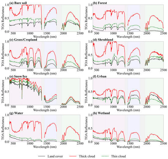
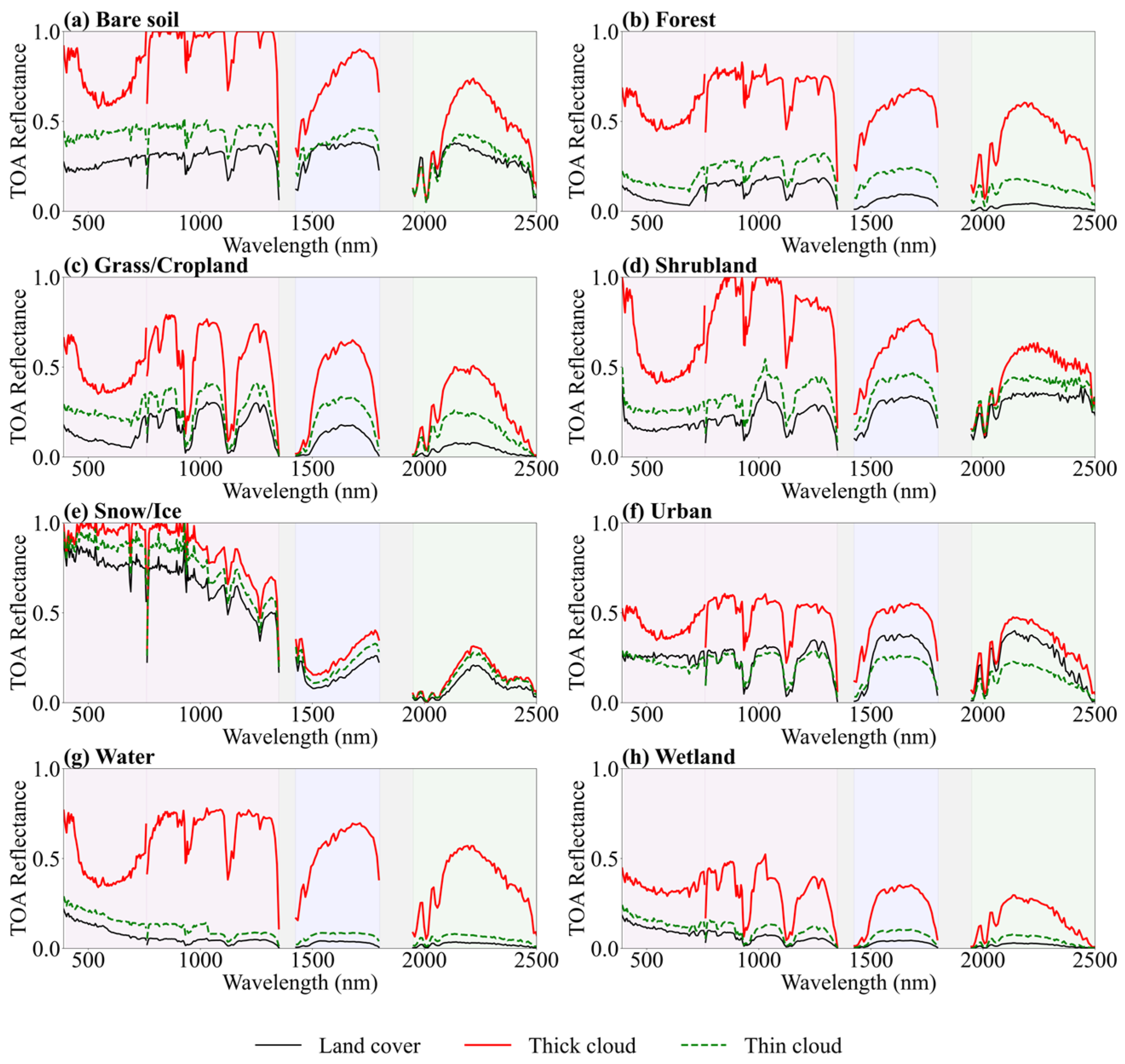
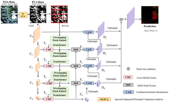
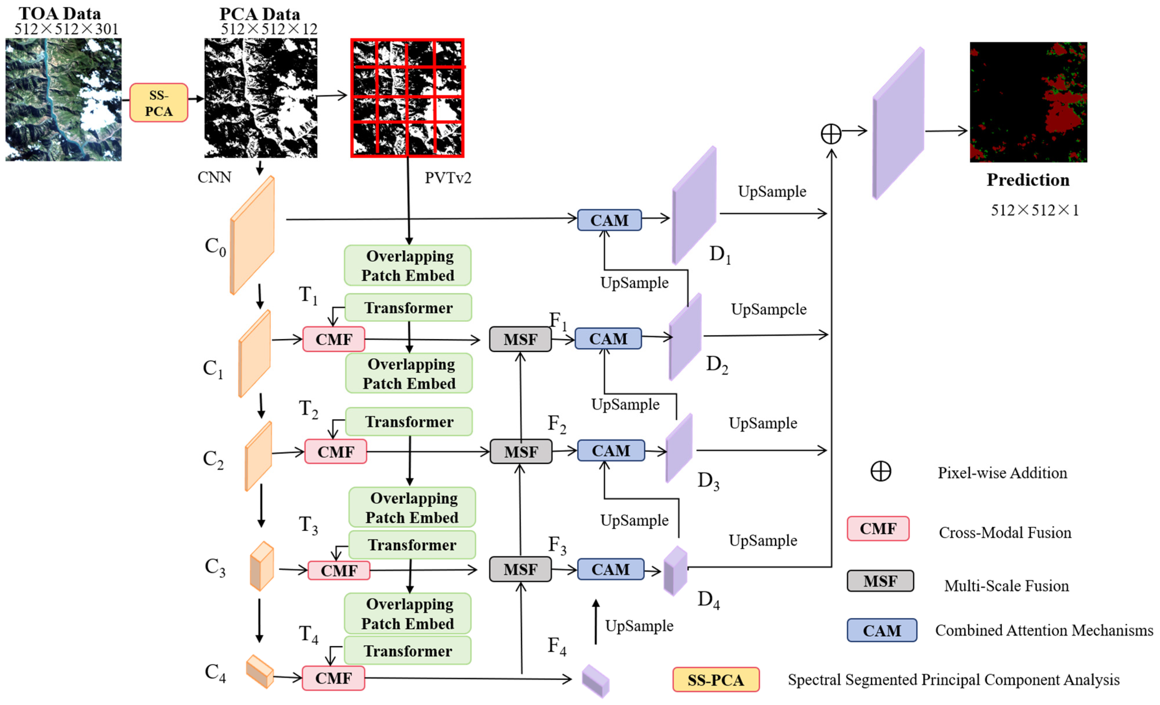
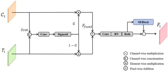
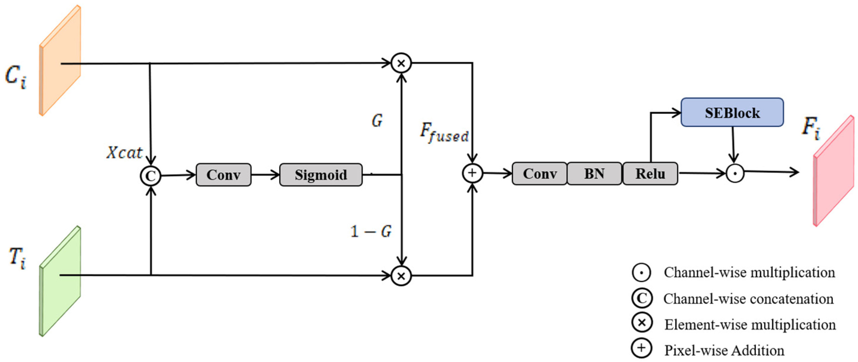
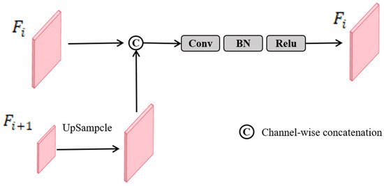
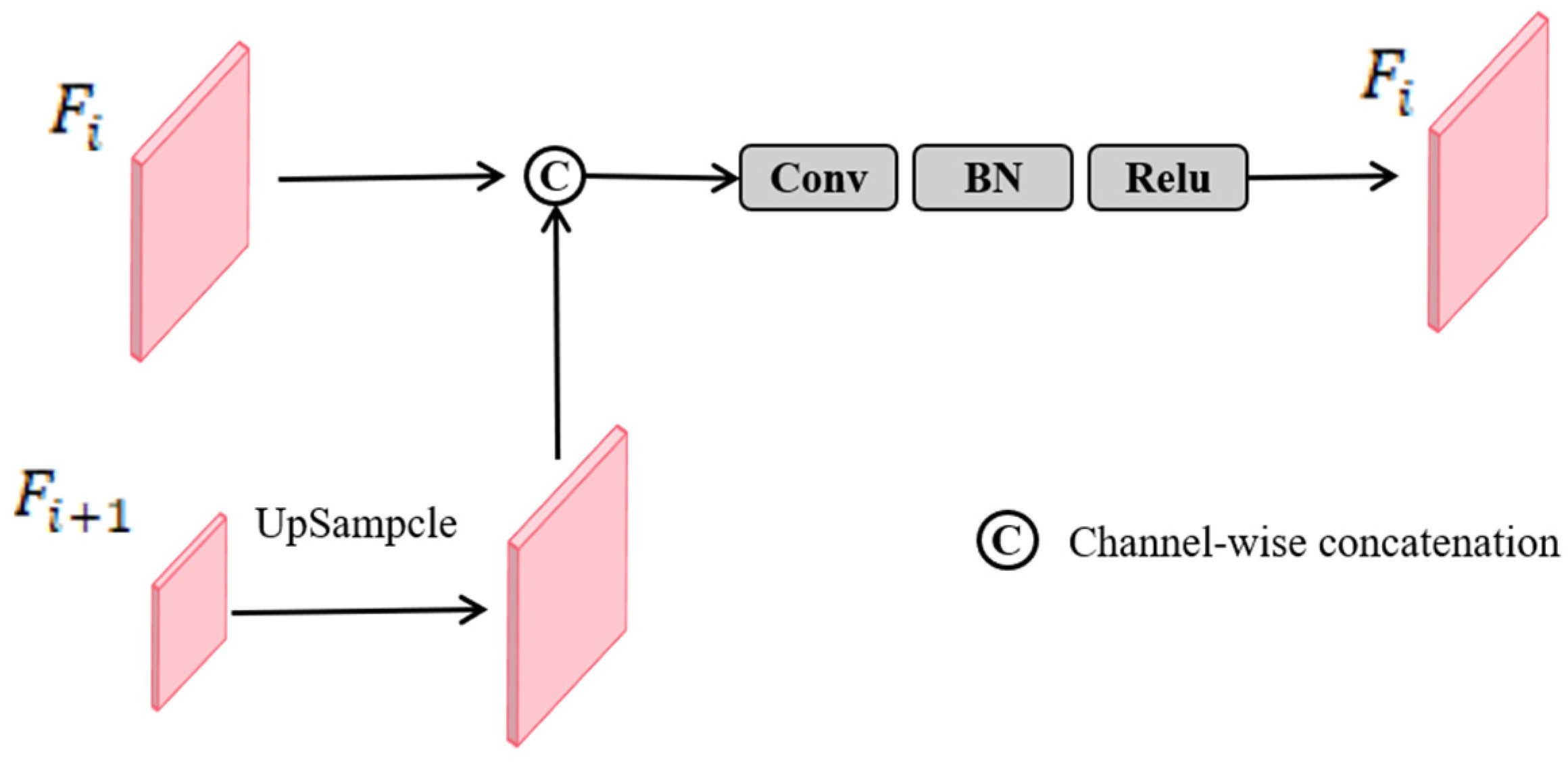
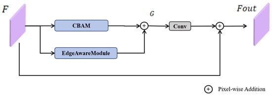
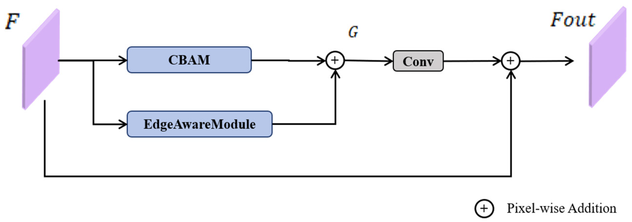
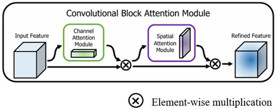
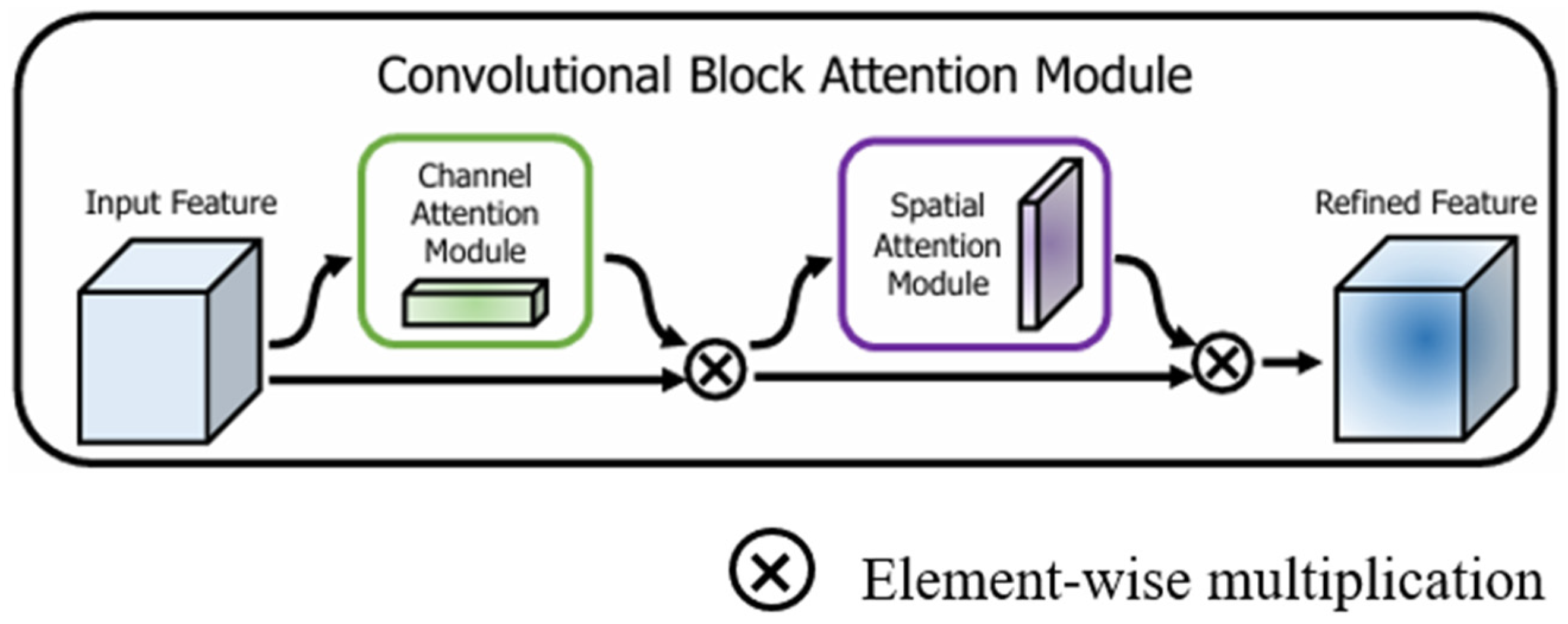
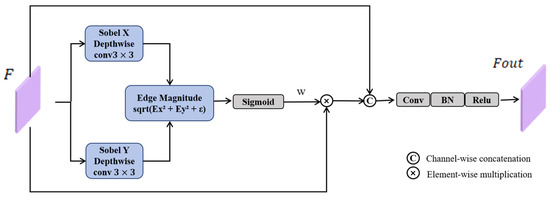
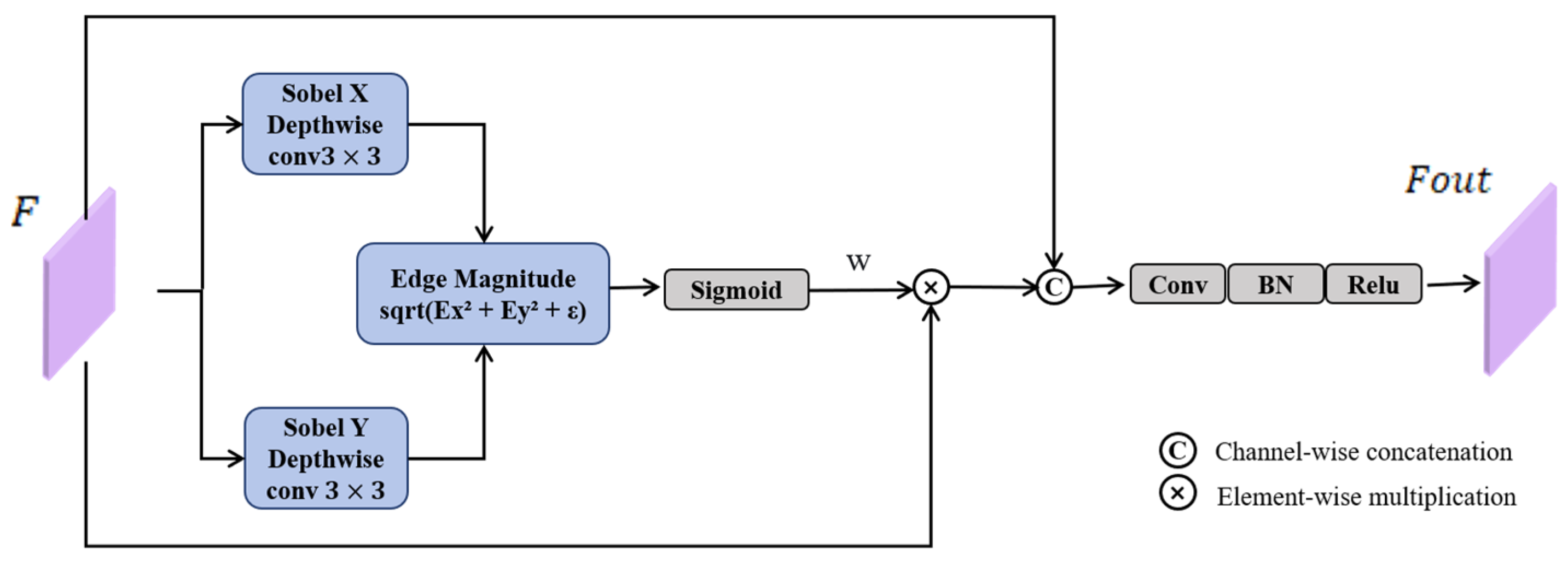
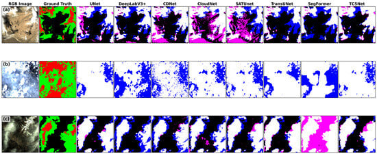
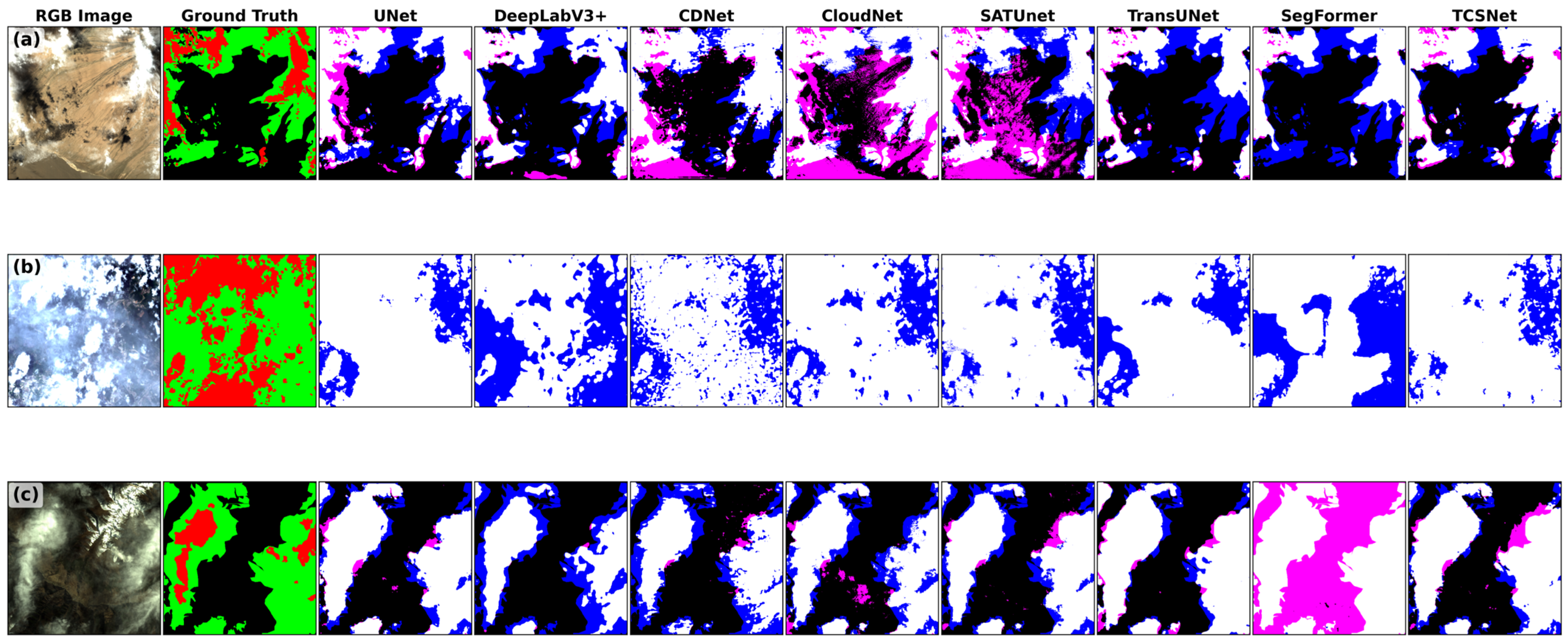
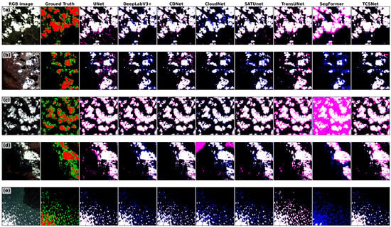
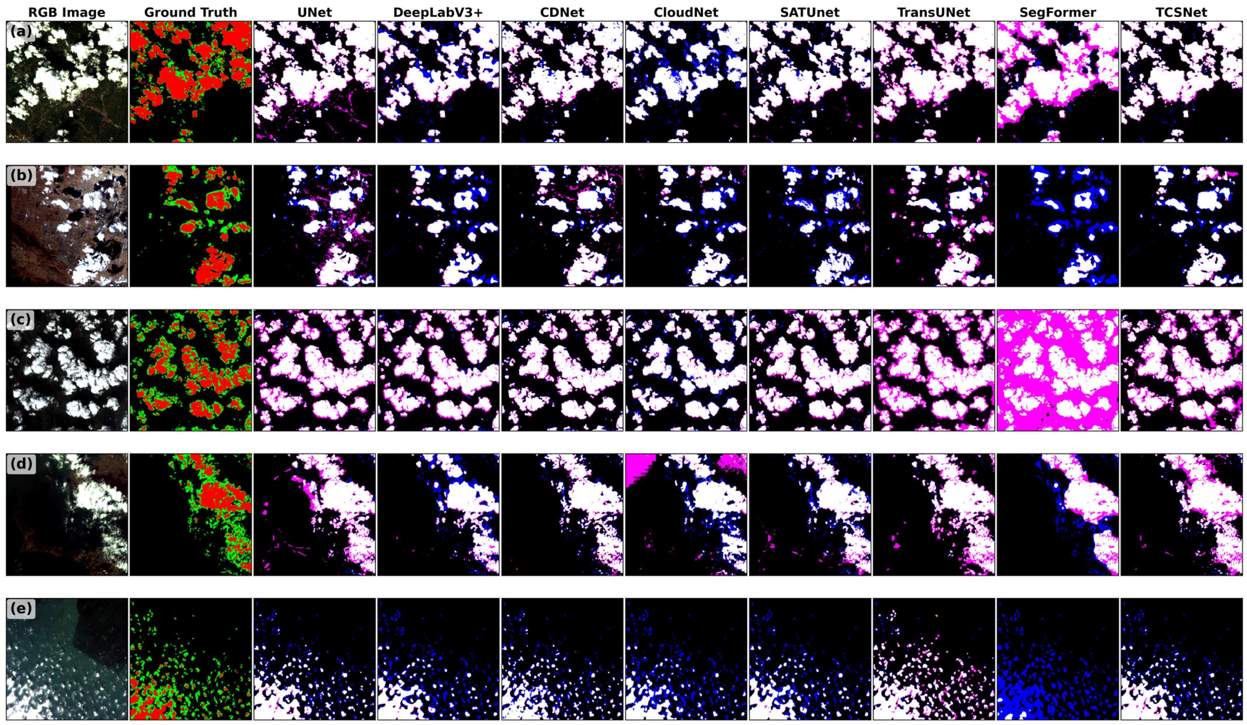
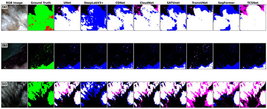
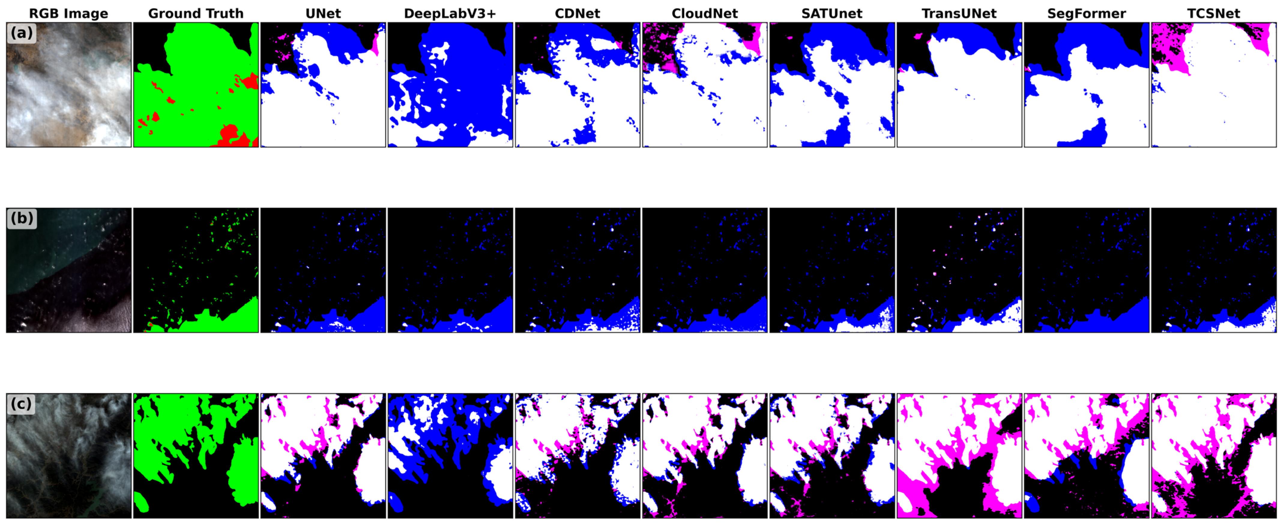

Disclaimer/Publisher’s Note: The statements, opinions and data contained in all publications are solely those of the individual author(s) and contributor(s) and not of MDPI and/or the editor(s). MDPI and/or the editor(s) disclaim responsibility for any injury to people or property resulting from any ideas, methods, instructions or products referred to in the content. |
© 2026 by the authors. Licensee MDPI, Basel, Switzerland. This article is an open access article distributed under the terms and conditions of the Creative Commons Attribution (CC BY) license.