


Highlights
What are the main findings?
- PIMSEL effectively integrates heterogeneous multi-modal geospatial data through physically guided optimal transport alignment and prototype-anchored graph clustering to assess post-seismic landslide reactivation risk under sparse supervision.
- Physically guided causal constraints and cross-modal semantic alignment contribute synergistically, with the latter identified as the single most critical design element for robust reactivation prediction.
What are the implications of the main findings?
- Calibrated uncertainty-aware prediction enables operational early warning systems to balance automated risk assessment with targeted human oversight, improving practical deployability in post-seismic environments.
- Embedding physical causality as architectural constraints enhances cross-regional generalizability, suggesting a scalable pathway for multi-modal geohazard risk management in data-scarce settings.
Abstract
Earthquake-induced landslide reactivation poses a sustained hazard for years following major seismic events, yet operational prediction remains constrained by heterogeneous multi-modal data, sparse supervision, and the absence of uncertainty-aware frameworks. This paper presents PIMSEL, a physically guided multi-modal semi-supervised framework for post-seismic landslide reactivation risk assessment. PIMSEL integrates satellite-derived morphological features, precipitation time series, and seismic hazard attributes through four components: entropy-regularized optimal transport for cross-modal semantic alignment without paired supervision; causally constrained hierarchical fusion enforcing domain-consistent modal weighting; scenario-based prototype mutation for semi-supervised learning from sparse expert annotations; and prototype-anchored variational graph clustering that simultaneously stratifies landslides into HIGH, MEDIUM, and LOW risk tiers and produces decomposed aleatoric and epistemic uncertainty estimates for operational triage. The HIGH risk tier operationally corresponds to predicted reactivation, validated against 598 documented reactivation events across 7482 co-seismic landslides from three Sichuan Province earthquake sequences: the 2013 Lushan (Mw 7.0), 2017 Jiuzhaigou (Mw 7.0), and 2022 Luding (Mw 6.8) events. PIMSEL achieves 82.5% reactivation recall and 66.4% precision, outperforming twelve baselines across clustering quality, classification, and uncertainty calibration metrics. Ablation studies confirm that optimal transport alignment contributes the largest individual performance gain. Current limitations include quarterly assessment frequency and dependence on optical imagery under cloud cover, which future integration of real-time meteorological triggers and SAR data should address.
1. Introduction
Earthquake-induced landslides represent a major secondary hazard in mountainous, seismically active regions, causing an estimated 40,000 to 80,000 fatalities worldwide over the past two decades. Large earthquakes frequently trigger tens of thousands of slope failures simultaneously, as demonstrated by the 2008 Wenchuan earthquake (Mw 7.9) and the 2015 Gorkha earthquake (Mw 7.8) [1,2,3]. Critically, landslide hazard persists well beyond the co-seismic phase: slopes destabilized by strong ground motion remain susceptible to reactivation for years under rainfall, aftershocks, and progressive material degradation [4,5]. Post-seismic reactivations are estimated to account for 40% to 60% of landslide-related casualties following major earthquakes, yet they remain substantially underrepresented in operational hazard assessments [6].
Existing approaches to reactivation prediction fall into three categories, each with fundamental limitations. Physics-based slope stability models provide mechanistic interpretability but require site-specific geotechnical parameters that are infeasible to obtain across thousands of earthquake-affected slopes [7]. Empirical rainfall threshold models offer computational efficiency but apply uniform thresholds across heterogeneous terrain, neglect seismic preconditioning, and produce false alarm rates exceeding 90% in operational systems [8,9]. Machine learning approaches have demonstrated strong performance in co-seismic landslide detection from optical or SAR imagery [10,11,12,13], and recent studies have extended these methods to susceptibility mapping using graph neural networks and uncertainty-aware frameworks [14,15]. However, these methods typically produce static susceptibility maps from single-modality inputs and require large, labeled datasets unavailable for reactivation analysis. Recent multi-modal fusion studies remain limited by naive feature concatenation, the absence of physically meaningful modal prioritization, and a lack of uncertainty quantification [16]. No existing framework jointly addresses heterogeneous data fusion, sparse label learning, and probabilistic risk estimation for post-seismic reactivation.
Addressing these gaps requires a framework that treats reactivation risk assessment as a unified three-part problem. The core task is semi-supervised risk stratification: partitioning earthquake-affected landslides into HIGH, MEDIUM, and LOW risk tiers using heterogeneous multi-modal observations under sparse expert supervision. The HIGH risk tier operationally corresponds to predicted reactivation, and framework performance is validated against 598 documented reactivation events across 7482 co-seismic landslides. Reliable risk stratification in this setting simultaneously requires: principled semantic alignment across heterogeneous modalities—satellite-derived morphological features, precipitation time series, and seismic hazard attributes—that differ fundamentally in spatial resolution, temporal sampling, and physical meaning; physically guided fusion that respects causal relationships between slope vulnerability, triggering conditions, and seismic preconditioning; effective propagation of sparse expert knowledge to unlabeled samples; and calibrated uncertainty estimates that distinguish irreducible observation noise from model uncertainty, enabling operational triage between automated and human-reviewed assessments.
To address these requirements, this paper proposes PIMSEL, a physically guided multi-modal semi-supervised framework for earthquake-induced landslide reactivation risk assessment, with four contributions. First, an entropy-regularized optimal transport module establishes cross-modal semantic alignment across the three heterogeneous modalities without requiring paired supervision, bridging the semantic gap that makes direct instance-level fusion unreliable. Second, a physically guided hierarchical fusion strategy enforces causally consistent modal weighting, reflecting the established causal hierarchy among slope vulnerability, precipitation triggering, and seismic preconditioning, contributing domain knowledge as an architectural constraint rather than relying solely on data-driven learning. Third, a scenario-based prototype mutation approach generates physically plausible synthetic reactivation scenarios in the fused embedding space, enabling effective semi-supervised learning from only 450 expert-labeled prototypes across 7482 landslide instances. Fourth, a prototype-anchored variational graph clustering model simultaneously performs risk stratification and produces decomposed aleatoric and epistemic uncertainty estimates, supporting a three-tier operational triage framework. The proposed framework is evaluated on three earthquake sequences from Sichuan Province, China—the 2013 Lushan (Mw 7.0), 2017 Jiuzhaigou (Mw 7.0), and 2022 Luding (Mw 6.8) events—and validated through a 16-month operational deployment following the Luding earthquake [12,14].
2. Related Work
2.1. Landslide Susceptibility and Hazard Assessment Methods
2.1.1. Physics-Based Approaches
Physics-based slope stability models provide mechanistic insights into landslide failure through explicit representation of geotechnical processes. Infinite slope analysis applies limit equilibrium theory to compute the factor of safety as the ratio of resisting to driving forces, requiring parameters such as cohesion, friction angle, and pore pressure [7,17]. Finite element methods, including PLAXIS and FLAC, extend this formulation by coupling hydro-mechanical processes to simulate progressive deformation and strain softening [18,19]. At regional scales, distributed models such as TRIGRS, SHALSTAB, and SINMAP combine slope stability theory with hydrological infiltration modeling to estimate spatially varying failure potential under rainfall forcing [20,21].
Despite strong physical interpretability, physics-based approaches face severe scalability constraints. Site-specific geotechnical parameters are rarely available for thousands of slopes across earthquake-affected regions. In addition, these models primarily address spatial susceptibility rather than temporal reactivation, as they lack integration with real-time triggering conditions and evolving post-seismic slope degradation. These limitations motivate data-driven methods capable of leveraging sparse observations while maintaining physical consistency.
2.1.2. Empirical and Statistical Methods
Empirical approaches establish statistical relationships between landslide occurrence and observable predictors without explicit physical modeling. Rainfall threshold models define intensity–duration relationships derived from historical landslide inventories and precipitation records [9,22]. Such models underpin operational early warning systems in several regions due to their computational efficiency and real-time applicability [8]. However, their site-agnostic nature results in high false alarm rates, often exceeding 90% in heterogeneous terrain [8,23]. Antecedent rainfall formulations incorporating precipitation history provide modest improvements [23,24] but remain threshold based.
Statistical susceptibility mapping methods, including logistic regression, discriminant analysis, and bivariate techniques, correlate landslide presence with topographic and geological factors [25,26]. While these approaches yield interpretable coefficients, they produce static susceptibility maps and cannot capture temporal dynamics or individual landslide evolution. The fundamental limitation persists: empirical methods lack slope-specific temporal modeling and cannot jointly integrate morphological state with evolving triggering conditions.
2.1.3. Machine Learning Approaches
Machine learning classifiers such as Random Forests and Support Vector Machines attempt to learn nonlinear thresholds [27,28] but remain limited by their reliance on aggregated predictors. Machine learning approaches have demonstrated improved performance through nonlinear feature learning. Shallow models, including Random Forests, Support Vector Machines, and Artificial Neural Networks, achieve high accuracy in susceptibility mapping using hand-crafted features derived from digital elevation models and thematic layers [26,29]. Deep learning architectures eliminate manual feature engineering through end-to-end training. Convolutional neural networks have been widely applied to landslide detection from optical satellite imagery, achieving high detection accuracy through hierarchical spatial feature extraction [27,28,29,30,31].
However, image-based deep learning methods typically produce binary detection or static susceptibility outputs without temporal modeling. Sequence models such as LSTM and RNN architectures capture rainfall–landslide temporal dependencies [32,33] but operate on precipitation data alone, neglecting morphological and seismic preconditioning. Recent multi-modal approaches fuse optical imagery and digital elevation models through simple concatenation [10,34]. These methods lack semantic alignment and do not impose physically meaningful prioritization among modalities. Moreover, most deep learning studies focus on co-seismic landslide mapping rather than post-seismic reactivation prediction [35,36]. No existing framework predicts which detected landslides will reactivate under future triggering conditions, particularly under sparse supervision and operational uncertainty requirements.
2.2. Multi-Modal Data Fusion for Geohazard Assessment
2.2.1. Multi-Source Remote Sensing Integration
Multi-source remote sensing integration aims to exploit complementary information from diverse sensors for landslide characterization. Fusion of optical and SAR data combines spectral and geometric information through feature-level or decision-level strategies [37,38]. While effective for landslide mapping, both modalities represent spatial information with similar semantics. Multi-temporal InSAR techniques enable millimeter-scale deformation monitoring over extended periods [39,40] but suffer from decorrelation in vegetated and rugged terrain, limiting applicability in earthquake-affected regions [41].
Multi-sensor platforms integrating optical imagery, thermal infrared data, and LiDAR-derived topography provide complementary measurements of surface properties [42,43]. However, most implementations employ simple layer stacking without learned cross-modal calibration. Precipitation observations from satellite and ground-based platforms are primarily incorporated into threshold-based warning systems, where rainfall acts as an external trigger rather than a semantically fused input [44,45]. Recent advances have demonstrated the value of physically guided precipitation estimation and downscaling for improving debris-flow warning in post-seismic mountainous environments [46]. As a result, existing fusion strategies largely focus on image-to-image integration and do not address fundamentally heterogeneous data types.
2.2.2. Spatio-Temporal Fusion Approaches
Spatio-temporal fusion models seek to capture dynamic processes by jointly modeling spatial and temporal patterns. Convolutional–recurrent architectures and 3D convolutional networks have shown success in flood and weather forecasting [47,48]. However, these models require dense temporal sampling, which is unavailable for landslide reactivation monitoring due to infrequent satellite revisits and coarse precipitation forecasts. Attention mechanisms provide adaptive feature weighting [49,50] and have been applied in medical imaging and landslide susceptibility mapping [51,52]. In geohazard applications, attention is typically limited to intra-modality feature selection rather than inter-modality semantic alignment.
Physics-guided machine learning incorporates domain knowledge through loss functions or architectural constraints, improving performance in climate and hydrological modeling [53,54]. Hybrid physics–ML landslide models constrain outputs using stability theory [55] but do not guide fusion weights among heterogeneous inputs. Representation learning frameworks from vision–language and audio–visual domains assume shared semantic spaces across modalities [56,57], an assumption violated by geohazard data where spatial imagery, temporal precipitation sequences, and seismic attributes represent distinct physical processes.
2.2.3. Cross-Modal Alignment Techniques
Cross-modal alignment methods address semantic correspondence across heterogeneous representations. Domain adaptation techniques align feature distributions across domains [58,59] and have been applied to transfer landslide susceptibility models between regions [60]. However, these methods operate within single modalities. Optimal Transport provides a principled framework for distribution alignment while preserving geometric structure [61,62] and has shown promise in computer vision and climate data harmonization [63]. Its application to multi-modal geohazard alignment remains unexplored. Correlation-based methods such as CCA require fully paired samples [64,65], while contrastive learning approaches depend on massive labeled datasets [66,67], both impractical for landslide reactivation. Consequently, no existing framework achieves principled semantic alignment across spatial, temporal, and structured geohazard data under sparse supervision.
2.3. Deep Clustering and Semi-Supervised Learning
2.3.1. Deep Clustering Methods
Deep clustering methods jointly optimize representation learning and clustering objectives. Traditional clustering algorithms operate on fixed features and lack end-to-end optimization [68,69]. Deep embedded clustering frameworks integrate autoencoders with soft assignment mechanisms [70], with extensions preserving local structure or enabling probabilistic clustering [71,72,73]. Contrastive clustering methods improve separability through self-supervised pre-training [74,75]. However, these approaches operate in fully unsupervised settings and ignore available expert knowledge. In landslide reactivation assessment, expert-labeled prototypes encode valuable domain knowledge but are extremely sparse. Existing deep clustering frameworks lack mechanisms to anchor representations to such prototypes while propagating risk categories to unlabeled samples.
2.3.2. Graph Neural Networks for Clustering
Graph neural networks enable semi-supervised learning by propagating labels through relational structures [76]. Applications to landslide susceptibility incorporate spatial dependencies between slope units [77]. Deep graph clustering and graph attention networks further enhance adaptability by learning graph structure and aggregation weights [78,79,80]. However, graph construction typically relies on geometric similarity, which fails to capture domain-specific relationships involving precipitation sensitivity, seismic preconditioning, and temporal evolution.
Few-shot learning methods compute class prototypes for efficient classification with limited labels [81] but do not exploit relational graph structure. The absence of prototype-anchored graph clustering frameworks limits the effective use of sparse expert annotations in large landslide inventories.
2.3.3. Uncertainty Quantification in Deep Learning
Uncertainty quantification is critical for operational geohazard systems. Bayesian deep learning and Monte Carlo dropout estimate epistemic uncertainty through stochastic inference [82], while uncertainty decomposition distinguishes data-driven and model-driven uncertainty sources [83]. Deep ensembles improve calibration at the cost of increased computation [84]. Post hoc calibration methods address overconfidence in neural networks [85]. Despite their importance, uncertainty-aware landslide models remain limited to static susceptibility mapping [86,87]. No existing framework provides uncertainty-aware, multi-temporal reactivation prediction that distinguishes between sparse observation uncertainty and model uncertainty.
2.4. Summary of Gaps
In summary, existing studies fail to jointly address four requirements for operational landslide reactivation prediction (Table 1): principled cross-modal semantic alignment, physically guided fusion weights reflecting causal relationships, efficient semi-supervised learning from sparse expert knowledge, and uncertainty-aware risk prediction. PIMSEL addresses all four gaps through the components described in Section 3.
Table 1.
Comparative analysis of landslide reactivation assessment methods.
3. Methodology
3.1. PIMSEL Framework Overview
PIMSEL is an end-to-end multi-modal framework that integrates satellite-derived morphological features, precipitation time series, and seismic hazard attributes to produce uncertainty-aware reactivation risk assessments for earthquake-induced landslides. The framework is organized into four functional stages as illustrated in Figure 1. The first stage extracts fixed-dimensional embeddings from each modality using pre-trained or trainable encoders, then projects them into a unified representation space. The second stage aligns these semantically disparate embeddings through entropy-regularized optimal transport (OT), establishing cross-modal correspondences without requiring paired supervision. The third stage fuses the aligned embeddings via a physically guided hierarchical mechanism that enforces causally consistent weighting among modalities. The fourth stage performs semi-supervised risk clustering by constructing a prototype-anchored graph, propagating sparse expert knowledge through graph convolution, and assigning probabilistic risk labels with decomposed uncertainty estimates via a variational framework.
Figure 1.
Overview of the PIMSEL framework.
PIMSEL introduces four contributions: OT-based cross-modal alignment across semantically heterogeneous modalities; physically guided hierarchical fusion with causally constrained weighting ; scenario-based prototype mutation in the fused embedding space to preserve physical plausibility under sparse supervision; and prototype-anchored variational graph clustering with calibrated uncertainty decomposition. Each component is detailed in the subsequent subsections.
3.2. Multi-Modal Data
Three complementary data sources including image, precipitation, and post shock seismic activities characterize the morphological state, temporal triggering conditions, and seismic hazard context of each landslide. Their acquisition and preprocessing procedures are described below.
3.2.1. Satellite Imagery
Satellite Imagery: Satellite imagery captures the current morphological vulnerability state of each landslide, encoding scarp geometry, material exposure, vegetation recovery, and surface consolidation. Images are acquired from Sentinel-2 (10 m resolution, 5-day revisit) and Landsat-8 (15 m pan-sharpened, 16-day revisit) via Google Earth Engine, covering the three study regions from April 2013 to December 2023. For each assessment at time T, sensor selection follows a strict priority rule: the latest cloud-free Sentinel-2 image within a 30-day window is selected first given its finer spatial resolution and more frequent revisit; Landsat-8 is used as a fallback only when no cloud-free Sentinel-2 image is available within the window. Same-season preference is applied within each sensor to ensure temporal consistency. When both sensors have cloud-free coverage, Sentinel-2 takes precedence. To harmonize spatial resolution across sensors before input to the morphological encoder, all selected images are resampled to a uniform 10 m ground sampling distance using bilinear interpolation within Google Earth Engine prior to patch extraction. In the rare case where neither sensor yields a cloud-free image within the 30-day window, the assessment timestamp is flagged as a data quality limitation and excluded from model evaluation; this accounts for the 29.7% of false negatives attributed to image staleness discussed in Section 5.2. Preprocessing then extracts 512 × 512-pixel RGB patches centered on each landslide centroid. Pixel values are normalized using ImageNet statistics; the rationale for this choice is tied to the morphological encoder described in Section 3.3. The output is a tensor .
3.2.2. Precipitation Time Series
Daily precipitation data encodes antecedent soil saturation state and short-term rainfall intensity, both of which are critical physical preconditions for landslide reactivation. Daily precipitation records are sourced from the Sichuan Province Meteorological Bureau, providing station-observed measurements across the three study regions at consistent temporal resolution. The precipitation data consists of point measurements from meteorological gauge stations, with an average inter-station spacing of approximately 15 to 30 km across the three study regions. This gauge network density is representative of operational monitoring networks in mountainous Sichuan and is consistent with station-observed records used in comparable post-seismic landslide studies in the region. A 90-day temporal window is constructed at each assessment time , comprising observed daily precipitation for days to . This window captures precipitation dynamics across three physically distinct timescales: the 3-day antecedent accumulation governing proximate pore pressure response [88], the 30-day antecedent accumulation reflecting seasonal soil moisture build-up [89], and the 90-day seasonal baseline establishing the dry-season onset context within which short-term rainfall anomalies are interpreted. This temporal structure captures two critical physical quantities: the Antecedent Precipitation Index (API), which quantifies cumulative soil moisture through exponentially weighted accumulation, and short-term rainfall intensity relative to the seasonal baseline. The computation of API can be expressed in Equation (1) as follows:
where denotes the daily precipitation for k days prior to the timestamp T. All 90 daily values are standardized to zero mean and unit variance using training-set statistics. The output is a vector .
3.2.3. Seismic Features
Seismic attributes capture the cumulative damage from the mainshock and the ongoing aftershock activity. The earthquake catalog for each study region is provided by the Institute of Engineering Mechanics, China Earthquake Administration (IEM-CEA), and the Sichuan Earthquake Administration (SEA), recording origin time, epicenter coordinates, focal depth, and magnitude for the mainshock and all subsequent aftershocks. Ground-motion parameters are obtained from USGS ShakeMap. From these sources, a 10-dimensional feature vector is constructed. Mainshock ground-motion intensity comprises three features—peak ground acceleration (PGA), cumulative absolute velocity (CAV), and Arias intensity—all interpolated at each landslide location from ShakeMap outputs. Aftershock activity over the preceding 3 months comprises five features derived from the IEM-CEA/SEA catalog: count of events within a 50 km radius, largest aftershock magnitude, Omori decay rate fitted to the observed sequence, cumulative seismic moment release, and days since the last event. Spatial and temporal context comprises two features: the minimum epicentral distance from any aftershock to the landslide location, and log-transformed days since the mainshock. Magnitude-related features are log-transformed, and all features are scaled to [0, 1] via min–max normalization over the training set.
3.3. Embedding Extraction
3.3.1. Morphological Encoder
The morphological encoder leverages the pre-trained BiFusion-LDSeg framework developed in our companion work for landslide segmentation. BiFusion-LDSeg employs dual-encoder architecture with ResNet (CNN) and Vision Transformer (ViT) branches, coupled through cascaded Bi-directional Attention Gates (Bi-AGs) that perform cross-modal feature calibration at multiple scales. The encoder output from the CNN branch has dimensions , while the ViT branch produces spatial embeddings with dimensions after the final Bi-AG fusion layer. Global average pooling (GAP) followed by a convolutional layer is applied across spatial dimensions to obtain a compact morphological embedding:
where and denotes the convolution that projects the concatenated dual-branch features to the final embedding dimension. The encoder remains frozen during PIMSEL training to preserve the learned landslide-specific spatial representations and prevent catastrophic forgetting. This embedding encodes multi-scale morphological vulnerability indicators including scarp geometry, material exposure patterns, vegetation recovery state, and surface consolidation degree. The architecture of the pre-trained morphological encoder is visualized in Figure 2 below.
Figure 2.
Morphological encoder architecture using frozen BiFusion-LDSeg.
3.3.2. Temporal Encoder
The temporal encoder employs the pre-trained TS2Vec model, a state-of-the-art framework for unsupervised time series representation learning. TS2Vec applies instance-level contrastive learning to capture temporal dependencies, seasonal patterns, and trend information without requiring task-specific labels. The 90-day precipitation sequence P is passed through the frozen TS2Vec encoder to obtain:
where . Freezing the encoder weights ensures that the learned temporal patterns generalize across different precipitation regimes. These embeddings capture three physically meaningful quantities from the observed precipitation window: antecedent soil saturation state through exponentially weighted cumulative accumulation over the full 90-day horizon, short-term rainfall intensity relative to the seasonal baseline through contrasts between recent and longer-term accumulations, and seasonal moisture context derived from the climatological pattern embedded within the 90-day observed record. No forecast precipitation data is used; all inputs are strictly observed historical measurements sourced from the Sichuan Province Meteorological Bureau as described in Section 3.2.2.
3.3.3. Seismic Encoder
The seismic encoder is a trainable three-layer multilayer perceptron (MLP) that adapts to the task-specific requirements of reactivation risk assessment. Unlike the morphological and temporal modalities where pre-trained encoders are available, seismic features are domain-engineered quantities that benefit from end-to-end learning. The architecture is:
where , , , and . Dropout regularization with rate prevents overfitting on the compact 10-dimensional input. This embedding encodes the cumulative seismic damage state, ongoing aftershock hazard, and spatio-temporal context of the post-seismic sequence.
The three encoders produce embeddings of different dimensionalities (512D, 320D, and 50D) that reflect the varying complexity and information content of each modality. Projection to a unified representation space is addressed in the following subsection.
3.4. Projection and Optimal Transport Alignment
The three encoders produce embeddings of heterogeneous dimensionality: , , . Direct concatenation or naive fusion would fail to account for the semantic gap between modalities—morphology describes spatial vulnerability, precipitation describes temporal triggering conditions, and seismic attributes describe hazard state. Although all three modalities are associated with the same landslide instances, instance-level identity does not imply semantic correspondence across modalities: a high-vulnerability morphological embedding may be semantically closer to a moderate-precipitation embedding than to the precipitation embedding of the same instance, because reactivation risk is governed by cross-modal physical relationships rather than instance co-occurrence. Direct instance-level fusion treats co-occurrence as semantic alignment, which produces spurious cross-modal associations and degrades clustering quality, as confirmed by the 13.4% performance gap between OT alignment and naive concatenation in our ablation experiments.
This subsection describes a two-stage process to establish a unified and semantically aligned representation space. Each embedding is independently projected to a shared 256-dimensional space via trainable two-layer MLPs. The projection architecture is identical across modalities to ensure dimensional consistency according to Equations (7) and (8):
where , with , , and the output embeddings , , are dimensionally aligned but semantically disparate. Layer normalization stabilizes training across the heterogeneous input scales, GELU activation provides smooth nonlinearity, and dropout prevents overfitting during projection learning.
While dimensional alignment enables concatenation, it does not resolve the semantic heterogeneity problem. The three modalities encode fundamentally different physical phenomena: represents what the landslide “is” (geometry, consolidation); represents what “will happen” (heavy rainfall), and represents what “continues to happen” (aftershock hazard). Optimal transport establishes cross-modal correspondences by treating each modality as a probability distribution over the feature space and finding the minimum-cost transport plan that aligns distributions [90]. Morphology is designated as the reference frame since it represents the baseline vulnerability state upon which triggers act. For each pair of modalities, a cost matrix quantifies pairwise Euclidean distances:
The optimal transport plan is computed via entropy-regularized optimal transport, solved efficiently using the Sinkhorn–Knopp algorithm. The full pseudocode for the Sinkhorn-OT alignment procedure is provided in Appendix A for reference. Here, the Sinkhorn algorithm iteratively refines the transport plan via alternating row and column normalizations, converging in 100 iterations. The computational complexity is where denotes the maximum number of Sinkhorn iterations. Once the transport plans and are computed, aligned embeddings are obtained via barycentric projection as expressed in Equations (11)–(13):
where the morphological embedding remains unchanged as the reference. The above computational details have been illustrated in Figure 3 below. The transport plans effectively reweigh precipitation and seismic features according to their relevance to each morphological state, establishing semantic correspondences that respect the underlying physical relationships between vulnerability, triggers, and hazard. Ablation experiments demonstrate that optimal transport alignment yields a 13.4% improvement in clustering quality compared to direct concatenation, confirming its importance in bridging the semantic gap between heterogeneous modalities.
Figure 3.
Optimal transport alignment for semantic correspondence. (a) Three-modality alignment. (b) Conceptual framework.
3.5. Physically Guided Hierarchical Fusion
This section describes a four-stage hierarchical fusion strategy (see Figure 4) that incorporates physical constraints to ensure the learned representations respect causal relationships between morphology, triggering conditions, and reactivation risk.
Figure 4.
Illustration of the proposed physically guided hierarchical fusion.
3.5.1. Spatial-Temporal Cross-Attention
Morphological vulnerability queries precipitation patterns to identify relevant temporal triggers. This asymmetric interaction reflects the physical principle that the effectiveness of precipitation as a trigger depends on the landslide’s structural state. Cross-attention is implemented via a single-head mechanism where morphology serves as the query and aligned precipitation serves as both key and value as expressed in Equations (14)–(16):
where project to a 64-dimensional attention space (), and the residual connection preserves the base morphological state. The attention mechanism learns which precipitation patterns are most relevant given the current vulnerability, encoding scenario-specific trigger sensitivities.
3.5.2. Multi-Head Attention Fusion
All available information is integrated via an 8-head multi-head attention mechanism operating over the concatenated modalities. The input comprises the spatial–temporal fused embedding, the aligned seismic embedding, and the original morphological and precipitation embeddings to preserve direct access to all signals:
where each head attends to the full modality set with separate learned projection matrices, projects the concatenated heads back to 256 dimensions and averaging over the modality dimension produces a compact attended representation. This stage captures complex inter-model dependencies that cannot be expressed through pairwise interactions alone.
3.5.3. Constrained Weighted Fusion
It is important to note that the physically guided constraint implemented here does not simulate geo-mechanical slope processes such as strength degradation or structural plane failure. Rather, it encodes physical causality as an architectural prior on modal contribution ordering, reflecting the established causal hierarchy among slope vulnerability, precipitation triggering, and seismic preconditioning documented in the post-seismic landslide literature [4,5,7]. This domain-consistent ordering constraint improves both model interpretability and generalizability by preventing the learning of physically implausible weight configurations, such as seismic contributions exceeding morphological vulnerability contributions in long post-seismic windows.
Domain knowledge dictates that morphology, precipitation, and seismic hazard contribute unequally to reactivation risk in the study region. Morphological vulnerability determines the capacity for failure and should receive the highest weight. Precipitation is the primary trigger in the monsoon-dominated Sichuan climate and should receive the second-highest weight. Seismic effects decay over time in the post-earthquake period and should receive the lowest weight. This ordering is enforced via a hard constraint on the learned fusion weights. Three raw weights are first normalized via softmax to ensure they sum to unity:
The constraint is enforced by sorting in descending order and reassigning:
During training, the learned weights converge consistently across three independent runs to , , and , confirming both the alignment of the constraint with data-driven signal importance and the stability of the weight learning process. The negligible standard deviations indicate that the physically guided ordering constraint produces reliable and reproducible modal weight assignments across different random initializations. Removing this constraint degrades performance by roughly 5%, as the unconstrained model occasionally learns physically implausible weight distributions such as .
3.5.4. Final Combination
The weighted embedding and the multi-head attention embedding capture complementary information—the former enforces physical priors while the latter learns data-driven dependencies. Both are concatenated and passed through a final MLP to produce the joint representation:
where , , , and the output serves as the fused multi-modal embedding for downstream clustering. This hierarchical design balances physical interpretability with representational flexibility, encoding both domain-constrained relationships and learned feature interactions within a unified framework.
3.6. Prototype-Anchored Graph Learning
The fused embeddings encode multi-modal reactivation risk signatures, but clustering directly in this space would ignore the valuable structural information present in the data manifold and the available expert-labeled prototypes. Graph-based learning addresses both limitations by constructing a similarity graph that captures local neighborhood structure and explicitly anchors unlabeled samples to expert-annotated scenarios. This section describes the graph construction process and the two-layer graph convolutional network that refines embeddings via neighborhood aggregation.
3.6.1. Graph Construction
A k-nearest neighbor graph is constructed over the N samples based on cosine similarity in the fused embedding space. First, embeddings are -normalized to ensure similarity is measured by angular proximity rather than magnitude (see Equation (26)) and the pairwise similarity matrix is computed as Equation (27):
To encourage connections between unlabeled samples and expert-labeled prototypes, similarities involving prototype nodes are boosted by 50 percent. Let denote the indices of the 450 expert prototypes. The boosted similarity matrix is:
Physical plausibility of synthetic samples is enforced through two mechanisms. A mutation radius constraint bounds each synthetic sample within a maximum Euclidean distance of 0.15 normalized embedding units from its source prototype, ensuring generated samples remain within the local neighborhood of physically validated expert scenarios. A physics-consistency filter subsequently discards any synthetic sample whose implied modal weight ordering violates the causally constrained hierarchy of Section 3.5.3, removing fewer than 3% of candidate mutations in practice. Distributional alignment between synthetic and real samples is confirmed by a mean cosine similarity of 0.91 in the fused embedding space, with 94.3% of synthetic samples falling within the convex hull of real samples, indicating that the synthetic expansion augments rather than distorts the true data manifold.
This modification increases the likelihood that each unlabeled sample connects to at least one expert-labeled scenario, facilitating label propagation. For each node i, the top-k most similar nodes are identified based on with . An additional constraint is enforced: if none of the 15 nearest neighbors are prototypes, the weakest connection is replaced with the nearest prototype to guarantee prototype anchoring. The adjacency matrix A is constructed such that where denotes the 15-neighborhood of node i. The graph is symmetrized and normalized via the standard symmetric normalization:
where is the degree matrix and is the normalized adjacency matrix used in graph convolution.
3.6.2. Graph Convolutional Network
A two-layer GCN refines embeddings by aggregating information from local neighborhoods, effectively smoothing the embedding space according to the graph topology [91]. Each layer applies a graph convolution followed by a nonlinear activation as expressed in Equations (32) and (33):
where are trainable weight matrices, dropout with rate prevents overfitting, and the output are graph-enhanced embeddings. The graph convolution operator aggregates features from each node’s immediate neighbors weighted by edge strength, effectively smoothing the embedding space according to the graph topology. The prototype-anchored structure ensures that expert knowledge propagates to nearby unlabeled samples [92]: if an unlabeled landslide is like a HIGH risk prototype, the GCN will incorporate the prototype’s representation into the landslide’s updated embedding, biasing it toward th4 HIGH risk region of the feature space. This semi-supervised mechanism leverages the 450 labeled prototypes to guide the organization of the 7482 unlabeled real landslides and 31,247 synthetic samples, improving clustering coherence without requiring exhaustive manual annotation. Ablation experiments demonstrate that the prototype-anchored graph yields a 6.5 percent improvement in clustering quality compared to direct clustering without graph-based refinement, confirming that the neighborhood structure and expert guidance meaningfully enhance representation learning. The overall prototype-anchored graph learning has been visualized in Figure 5 below.
Figure 5.
Scenario-based prototype mutation and graph-based semi-supervised learning.
3.7. Variational Clustering
The graph-enhanced embeddings must be partitioned into three risk categories (HIGH, MEDIUM, and LOW) while quantifying the uncertainty in each assignment. A variational autoencoder framework addresses both objectives by learning a probabilistic latent space structured according to a Gaussian mixture model prior. This section describes the encoder–decoder architecture, the cluster assignment mechanism, the five-component loss function, and the dual uncertainty decomposition strategy.
3.7.1. Variational Encoder
The encoder maps graph-enhanced embeddings to a probabilistic latent space by predicting a Gaussian distribution for each sample. A two-layer MLP processes the input:
where , , and . Two separate branches predict the mean and log-variance:
where and . The latent code is sampled via the reparameterization trick to enable backpropagation through the stochastic node:
where denotes element-wise multiplication. The latent code serves as the input to both the cluster assignment network and the decoder.
3.7.2. Cluster Assignment Network
A linear classifier maps latent codes to cluster membership probabilities:
where , , and represent the probability distribution over the three risk levels. The discrete cluster assignment is obtained as where .
3.7.3. Gaussian Mixture Model Prior
The latent space is structured according to a three-component GMM prior with one component per risk level [93]. Each component is characterized by a mean , a diagonal covariance matrix , and a prior probability . The GMM parameters are initialized using the expert prototypes: is set to the empirical mean of the graph-enhanced embeddings of all prototypes with label , and is initialized to the identity matrix. During training, the GMM parameters are updated every 10 epochs via an expectation-maximization step using the current cluster assignments:
where is the soft cluster size. A momentum coefficient of 0.9 is applied to stabilize updates: . The GMM prior encourages the latent space to organize into three well-separated, Gaussian-distributed clusters corresponding to the risk levels.
3.7.4. Decoder
The decoder reconstructs the graph-enhanced embedding from the latent code to ensure the latent space preserves information content:
where , , and is the reconstructed embedding. The reconstruction target is .
3.8. Uncertainty Quantification
Two complementary types of uncertainty are estimated [94]. Aleatoric uncertainty captures irreducible noise in observations and is derived from the encoder variance as expressed in Equation (46):
Epistemic uncertainty captures model uncertainty via Monte Carlo dropout with forward passes. During each pass, dropout is enabled in the encoder and cluster assignment network, producing a sample prediction . The mean prediction and per-class variance are:
Total uncertainty is measured via the entropy of the mean prediction as expressed in Equation (50):
The final cluster assignment uses the mean prediction with confidence . Samples with confidence greater than 0.8 are designated for automated processing, those between 0.6 and 0.8 for semi-automated expert review, and those below 0.6 for manual assessment. This triage strategy enables operational deployment with 63.5 percent of assessments fully automated while maintaining human oversight on uncertain cases.
3.9. Loss Functions
Training optimizes a weighted combination of five loss terms: The cluster assignment loss encourages latent codes to fit the GMM components; the reconstruction loss ensures the latent space preserves information; the KL divergence loss regularizes the posterior distribution toward the GMM prior; the graph smoothness loss enforces that connected nodes have similar latent representations; and the prototype supervision loss applies cross-entropy on the 450 labeled prototypes and 31,247 labeled synthetic samples, denoted by index set . They are expressed in Equations (51)–(55) in detail:
where is the ground-truth label. The total loss function can be expressed in Equation (56):
with weights determined via cross-validation. The high weight on reflects the value of expert-labeled data in anchoring the cluster structure.
4. Experimental Results
4.1. Dataset Preparation
Experiments are conducted on three earthquake-triggered landslide inventories from Sichuan Province, China (Table 2). The Lushan earthquake produced the most spatially distributed landslide inventory, spanning eight counties with concentration in Lushan County (6501 instances) and Baoxing county (4775 instances). Jiuzhaigou triggering was spatially confined to a single county (4834 instances), consistent with the narrower rupture extent of the 7.0 event. The Luding inventory is split primarily between Shimian (3020) and Luding (1981) counties, reflecting bilateral rupture along the Xianshuihe fault.
Table 2.
Co-seismic landslide inventory by county for the three earthquake events.
Within three months of the Lushan mainshock (as shown in Figure 6), 814 aftershocks of were recorded, including 40 events at and a maximum of 5.4 on 21 April; focal depths range from 0.23 to 33.33 km (mean 12.17 km). The Jiuzhaigou sequence produced 673 aftershocks with a maximum of 4.9 on 9 August and notably shallow focal depths (mean 5.92 km, range 0.02–65.35 km). The Luding sequence was the least active, with 566 aftershocks, only 3 events at , a maximum of 5.2 on 22 October, and mean focal depth of 9.26 km. The progressive attenuation visible across all three panels directly motivates the exponential seismic weight decay incorporated in PIMSEL’s physically guided fusion (Section 3.5), and the three-year daily rainfall time series is shown in Figure 7.
Figure 6.
Aftershock sequences within three months post-mainshock for the three study earthquakes: (a) Lushan ( 7.0, 2013), (b) Jiuzhaigou ( 7.0, 2017), and (c) Luding ( 6.8, 2022).
Figure 7.
Three-year daily rainfall time series (including the earthquake year). (a–h) represent the counties involved in the Lushan Earthquake; (i–l) represent the counties involved in the Luding Earthquake; and (m) represents the county involved in the Jiuzhaigou Earthquake.
4.2. Evaluation Metrics and Implementation Details
PIMSEL is evaluated against twelve baselines spanning four categories (Table 3). All methods operate on identical input data across three modalities, with hyperparameters independently tuned via grid search on the validation set under an 80%/10%/10% training/validation/test split. Performance is assessed across two clustering quality metrics: Silhouette Score (Equation (57)) and Davies–Bouldin Index (Equation (58)). Also, two classification metrics including Cohen’s (Equation (59)) and macro F1-score (Equation (60)), and two uncertainty calibration metrics including ECE (Equation (61)) and Brier score (Equation (62)) are all evaluated with formulations consistent with the variable notation of Section 3 as follows.
Table 3.
Summary of baseline methods.
The Silhouette Score quantifies the ratio of inter-cluster separation to intra-cluster cohesion per sample, with the overall score computed as the mean over all samples; values range from [−1, 1] with higher values indicating better-defined clusters. The Davies–Bouldin Index (DBI) measures the average ratio of within-cluster scatter to between-cluster distance across all risk clusters, where denotes the mean distance of samples in cluster to their centroid and denotes the Euclidean distance between centroids; lower DBI values indicate superior cluster separation, directly reflecting the quality of the GMM latent space (Section 3.7.3). Cohen’s measures chance-corrected agreement between predicted cluster assignments and expert risk labels, where is the observed agreement proportion and is the expected agreement under chance. The macro-averaged F1-score is the unweighted mean across three classes, and overall accuracy is the proportion of correctly assigned instances across all labeled test samples. ECE quantifies the alignment between predicted confidence and empirical accuracy across confidence bins, where denotes the set of samples within bin , is the empirical accuracy, and is the mean predicted confidence; lower ECE reflects better calibration of the decomposed uncertainty estimates described in Section 3.8. The Brier score provides a complementary probabilistic accuracy measure, where denotes the predicted probability for class k from the cluster assignment network (Equation (41)) and is the ground-truth indicator.
The framework is implemented in PyTorch 2.0.1 with PyTorch Geometric 2.3.1 and POT 0.9.0, trained on a single NVIDIA A100 GPU (40 GB). The morphological and temporal encoders are kept frozen at their pre-trained weights; all remaining components are jointly optimized via Adam (, cosine annealing, batch size 128) for up to 300 epochs with early stopping. Loss weights , , , are determined via five-fold cross-validation on the Lushan training set. OT regularization is set to with 100 maximum Sinkhorn iterations, and graph neighborhood size to . All results are averaged over three independent runs with random seed 42.
4.3. Clustering Quality and Performance Comparison
4.3.1. Morphological Embedding
The morphological embeddings input to PIMSEL are derived from BiFusion-LDSeg [96], a latent diffusion segmentation framework with bi-directional CNN-Transformer fusion trained on the same three earthquake datasets. Prior to presenting clustering results, Figure 8 validates the quality of these upstream embeddings through representative segmentation outputs. Across nine cases spanning diverse landslide morphologies including debris flows in Lushan, compact rotational slides in Jiuzhaigou, and irregular mixed-type failures in Luding. Here, BiFusion-LDSeg produces boundary delineations that closely follow the ground truth, achieving an IoU of 68.5%, 70.8%, and 68.3% on the three datasets, respectively [96]. Residual errors are confined primarily to low-contrast woodland margins, consistent with known optical imagery limitations under dense canopy cover. The strong segmentation fidelity across all three regions confirms that the frozen morphological encoder transferred to PIMSEL carries reliable geometric and textural representations of slope vulnerability, forming a robust foundation for the subsequent multi-modal risk clustering.
Figure 8.
Representative BiFusion-LDSeg segmentation results for nine landslide instances (three per study region).
4.3.2. PIMSEL Assessment Performance
After incorporating the morphological embeddings with the precipitation embeddings and seismic embeddings, the proposed PIMSEL achieves state-of-the-art performance across all metrics (Table 4). The Silhouette Score of 0.634 represents a 17.0% improvement over the strongest baseline, GraphST (0.542), attributable to the combined effect of optimal transport alignment, physically guided fusion, and prototype-anchored graph learning. The DBI of 1.072 is 16.6% lower than the best baseline value of 1.285 (IDEC), confirming superior inter-cluster separation relative to intra-cluster scatter in the learned latent space.
Table 4.
Overall performance comparison across all methods.
Classification performance on the held-out labeled test set further validates the quality of the learned representations. Cohen’s of 0.768 indicates strong agreement with expert risk assignments, outperforming GraphST by 9.6% (). The macro-averaged F1-score of 0.826 reflects balanced performance across risk categories, with overall accuracy of 82.9% on 867 labeled test samples. Statistical significance is confirmed via paired t-tests against all twelve baselines (), with McNemar’s test further validating classification improvements (). Bootstrapped 95% confidence intervals over 1000 resamples show no overlap between PIMSEL and the strongest baseline.
Figure 9 presents t-SNE visualizations of the learned embeddings for three representative baselines and PIMSEL, stratified by study region. PIMSEL exhibits clear inter-cluster separation with minimal boundary overlap, whereas baseline methods show substantial inter-cluster mixing, particularly between the MEDIUM and HIGH risk classes. This confirms that physically guided hierarchical fusion and prototype-anchored graph learning encode risk-relevant structure that unconstrained attention mechanisms fail to capture.
Figure 9.
t-SNE visualizations of learned latent embeddings on the test set.
4.3.3. Comparison with Baseline Methods
Traditional clustering methods (K-Means, GMM, and DBSCAN) on concatenated features yield –, underscoring the inadequacy of feature-space concatenation without semantic alignment. Deep clustering methods improve substantially—DEC (), IDEC (), and VaDE ()—yet the absence of graph aggregation and cross-modal alignment leaves a 9.8–15.8% gap relative to PIMSEL. Graph-based methods narrow this gap: GraphST (), the strongest baseline, falls only 8.7% short of PIMSEL despite lacking physics constraints and OT alignment, though it learns physically implausible modal weights () in approximately 12% of training epochs. Among multi-modal baselines, Concat+K-Means () isolates the cost of dimensional misalignment, while Attn Fusion+VaDE ()—the closest multi-modal competitor—demonstrates that unconstrained attention alone is insufficient, with the 6.8% remaining gap attributable to the absence of physics constraints and OT alignment. Figure 10 shows PIMSEL ranking first across all metrics, with the largest margins in Silhouette Score (+17.0%) and DBI (−16.6%).
Figure 10.
Silhouette Score comparison across all baselines evaluated methods.
4.3.4. Per-Class Performance Analysis
Per-class metrics (Table 5, Figure 11) are balanced across all risk levels—HIGH (precision 81.2%, recall 82.0%, F1 81.6%, ), MEDIUM (77.2%, 82.5%, 79.8%, ), and LOW (83.9%, 83.9%, 83.9%, )—with macro-averaged precision, recall, and F1 of 80.8%, 82.8%, and 81.8% despite natural test imbalance (HIGH 23.6%, MEDIUM 36.3%, and LOW 40.0%).
Table 5.
Per-class performance metrics for PIMSEL.
Figure 11.
Per-region confusion matrices and per-class performance metrics for PIMSEL.
Three principal misclassification patterns emerge from the confusion matrix. HIGH → MEDIUM errors (32 cases, 15.6%) are predominantly borderline: 65.6% fall in the 0.55–0.65 confidence band, making them natural candidates for semi-automated expert review rather than outright misclassification. MEDIUM → LOW errors (27 cases, 8.6%) trace to underrepresentation of localized convective rainfall extremes in station-observed records. Post hoc substitution of spatially interpolated precipitation reclassifies 66.7% of these cases correctly, pointing to a systematic data coverage gap rather than a model deficiency. LOW → MEDIUM errors (45 cases, 13.0%) are operationally preferable false positives concentrated in Lushan (68.9%), suggesting potential for region-specific threshold adjustment.
Regional analysis reveals distinct misclassification patterns across the three study areas (Table 6). Lushan contributes the largest share of total errors (59 of 104, 56.7%), consistent with its larger test sample count and more diverse terrain. HIGH → MEDIUM errors are distributed relatively evenly across regions, confirming that borderline cases reflect a systematic challenge rather than a region-specific phenomenon. MEDIUM → LOW errors show moderate concentration in Lushan (44.4%), attributable to the more complex precipitation patterns in the Ya’an region where station-observed records may underrepresent localized convective events. LOW → MEDIUM false positives are strongly concentrated in Lushan (68.9%), suggesting that region-specific threshold adjustment for morphologically active but hydrologically stable slopes could meaningfully reduce this error category. Jiuzhaigou and Luding show comparably low error rates (9.6% and 7.9%, respectively), likely reflecting their more spatially confined rupture extents and more homogeneous terrain conditions.
Table 6.
Regional distribution of misclassifications across the three study areas.
HIGH class recall of 82.0% exceeds GraphST (73.2%) and VaDE (78.5%) by 8.8 and 3.5 percentage points, respectively, corresponding to 18 additional correct identifications. The 37 remaining false negatives decompose into three failure modes: rapid-onset events within two weeks (37.8%), precipitation intensity extremes exceeding the 90th percentile of station-observed records (32.4%), and data quality degradation from image staleness beyond 45 days or sensor anomalies (29.7%). The recall advantage over GraphST originates from physically guided fusion amplifying morphological vulnerability signals under moderate trigger conditions. GraphST over-weights transient low-magnitude aftershocks (M less than 3.5) that carry little predictive value beyond the early post-seismic period. The 6.1 percentage-point LOW precision gain reflects the seismic weight decay modeled in Section 3.5, which appropriately suppresses seismic contributions beyond three months post-mainshock.
4.4. Reactivation Detection and Trigger Attribution
4.4.1. Overall Performance
PIMSEL correctly predicts 493 of 598 documented reactivations prior to event onset, achieving 82.5% recall—the primary operational metric for early warning systems. Performance varies by region: Lushan 87.4% (320/366), Jiuzhaigou 77.2% (88/114), and Luding 81.4% (96/118). The 105 false negatives (17.5%) decompose by failure mode: rapid-onset events within two weeks (Type 1, 41 cases, 39.0%), precipitation intensity extremes exceeding the 90th percentile of station-observed records, likely reflecting sparse gauge coverage of localized convective events (Type 2, 47 cases, 44.8%), and data quality issues including image staleness or catalog gaps (Type 3, 17 cases, 16.2%).
Of 742 HIGH risk predictions, 249 are false positives (33.6% false alarm rate, 66.4% precision). Many correspond to landslides that were mobilized but stabilized before failure—operationally preferable to missed warnings given the asymmetric cost structure of early warning decisions. PIMSEL’s 82.5% recall exceeds GraphST (73.8%) and VaDE (79.1%) by margins equivalent to 52 and 20 additionally correctly predicted events.
4.4.2. Uncertainty Calibration
The ECE of 0.042 confirms close correspondence between predicted probabilities and observed frequencies, substantially outperforming GraphST (ECE = 0.127) and VaDE (ECE = 0.089) (Figure 12). The reliability diagram shows near-diagonal correspondence across all confidence bins: predictions in the 0.8–1.0 range achieve 91.2% empirical accuracy (), while the 0.6–0.8 range yields 72.4% (). These bands directly support a three-tier operational triage: automated processing for high-confidence assessments (>0.8, 63.5% of cases), semi-automated expert review for medium-confidence cases (0.6–0.8, 27.0% of cases), and full manual assessment for low-confidence predictions (<0.6, 9.5% of cases). This triage structure confirms that the dual uncertainty decomposition, aleatoric uncertainty from encoder variance (Equation (46)) and epistemic uncertainty from MC dropout (Equation (49)) provide reliable operational guidance rather than nominal probabilistic output.
Figure 12.
Reliability diagrams comparing uncertainty calibration.
Decomposed uncertainty analysis reveals distinct signatures across error types. HIGH class false negatives () exhibit elevated epistemic uncertainty (mean = 0.31 vs. 0.14 for true positives), with 78.4% exceeding the 75th percentile threshold, indicating that model ambiguity rather than irreducible data noise drives these failures. LOW → MEDIUM false positives show the opposite pattern that elevated aleatoric uncertainty (mean = 0.28 vs. 0.16 for true negatives) implicates precipitation forecast variability and data quality as the dominant factors. This distinction has direct operational implications: high epistemic uncertainty cases are best addressed through additional prototype labeling or region-specific fine-tuning, while high aleatoric uncertainty cases call for improved data acquisition via shorter revisit cycles, SAR augmentation, or multi-model precipitation ensembles. During the 16-month Luding deployment, 149 of 189 medium-confidence predictions (78.8%) were confirmed or refined through expert review, validating the practical utility of the triage framework.
4.4.3. Trigger Attribution and Case Study
Trigger attribution achieves 76.2% accuracy across 467 cases with unambiguous ground truth (91 ambiguous cases excluded). Precipitation-dominated events () are attributed correctly in 81.0% of cases (234/289), with most errors (38/55, 69.1%) arising from over-attribution to combined rather than purely precipitation triggers. Seismic-dominated events () yield 73.2% attribution accuracy (104/142), with errors typically reflecting under-weighting of morphological preconditioning. Combined-trigger events () are the most difficult to classify (61.1%, 22/36), consistent with their inherent physical ambiguity.
Figure 13, Figure 14 and Figure 15 present three reactivation cases from the Lushan and Jiuzhaigou earthquakes, illustrating how PIMSEL captures the transition from seismic-dominated to precipitation-dominated trigger regimes as post-seismic conditions evolve. Case I (Figure 13; Guanjiagou landslide, Baoxing County, reactivated 19 June 2013) occurs approximately two months post-mainshock under residual seismic forcing and moderate cumulative precipitation. PIMSEL correctly assigns HIGH risk from the initial assessment through confirmed displacement, with seismic preconditioning identified as the dominant trigger given the proximity to the mainshock. Case II (Figure 14; Shuilierpingzi landslide, Lushan County, reactivated 7 May 2013) reactivates 17 days post-mainshock under combined aftershock activity (Mw 3.7) and moderate daily precipitation (17.5 mm). PIMSEL correctly weights both seismic preconditioning and rainfall accumulation, maintaining HIGH risk assignment from the immediate post-seismic period through reactivation. Case III (Figure 15; Chaoyang Village landslide, Jiuzhaigou County, reactivated 29 September 2017) demonstrates delayed monsoon-season reactivation 52 days post-mainshock. Progressively increasing daily precipitation across three assessment nodes drives trigger attribution to shift entirely from seismic to precipitation, with near-zero seismic contribution at the final node, confirming that PIMSEL’s physically guided seismic weight decay correctly captures post-seismic trigger regime evolution. Together, these three cases confirm that PIMSEL’s physically guided seismic weight decay correctly suppresses aftershock contributions on the timescale of weeks to months, while precipitation sensitivity increases as antecedent moisture accumulates.
Figure 13.
Case I (Lushan earthquake): Guanjiagou landslide, Mupingzhen, Baoxing County, Ya’an (reactivated 19 June 2013).
Figure 14.
Case II: Shuilierpingzi landslide, Zhongling Village, Taiping Town, Lushan County (reactivated 7 May 2013).
Figure 15.
Case III: Chaoyang Village landslide, Shuanghe Town, Jiuzhaigou County (reactivated 29 September 2017).
Figure 16, Figure 17 and Figure 18 present the remaining three cases from the Jiuzhaigou and Luding earthquakes, spanning the full range of post-seismic trigger regimes. Case IV (Figure 16; Langzhai Village, Jiuzhaigou County, reactivated 17 August 2017) fails only 9 days post-mainshock under near-zero precipitation, with PIMSEL correctly attributing HIGH risk to shallow seismic forcing at epicentral distances as close as 0.6 km. This represents a scenario that precipitation-threshold methods would systematically miss. Case V (Figure 17; Hongtazi landslide, Kangding County, reactivated 11 September 2022) represents a combined-trigger event in the early post-seismic window, where moderate aftershock activity and light-to-moderate precipitation contribute comparably to the HIGH risk prediction, demonstrating PIMSEL’s capacity to handle ambiguous multi-trigger scenarios. Case VI (Figure 18; Zhengjia’ping landslide, Shimian County, reactivated 16 July 2023) reactivates 10 months post-mainshock under purely precipitation-driven conditions with daily totals reaching 65.0 mm against zero recorded seismic activity. Together with Case IV, this confirms that PIMSEL’s time-varying modal weighting correctly spans the full post-seismic trigger spectrum from seismic-dominated to precipitation-dominated regimes. The contrast between Cases IV and VI, both from the Luding sequence yet separated by ten months and representing opposite ends of the trigger spectrum, directly validates the time-varying modal weighting scheme described in Section 3.5.
Figure 16.
Case IV: Langzhai Village landslide, Zhangzha Town, Jiuzhaigou County (reactivated 17 August 2017).
Figure 17.
Case V: Hongtazi landslide, Nanwu Village, Yulin Sub-district, Kangding County (reactivated 11 September 2022).
Figure 18.
Case VI: Zhengjia’ping landslide, Xingfu Village, Wanggangping Town, Shimian County (reactivated 16 July 2023).
4.5. Ablation Studies
4.5.1. Component-Wise Contribution Analysis
Incremental addition experiments (Figure 19a–c) trace individual component contributions from a baseline of concatenation + K-Means (). Projection networks add +3.1% (), OT alignment +14.8% (), physically guided fusion +5.3% (), scenario mutation +3.4% (), graph anchoring +6.8% (), and VaDE clustering +6.5% (), for a cumulative gain of +46.8%. The dominant contribution of OT alignment (+14.8%) confirms that cross-modal semantic correspondence is the single most critical design choice, outweighing dimensional alignment alone.
Figure 19.
Component-wise ablation results for the three study regions.
Component removal ablation (Figure 19d–f) corroborates this hierarchy. OT alignment removal causes the largest degradation (, −14.5%), followed by prototype anchoring (, −11.6%), graph structure (, −8.5%), physics constraints (, −6.8%), and scenario mutation (, −3.9%). Removing MC dropout leaves cluster quality unchanged () while increasing ECE from 0.042 to 0.089, isolating uncertainty quantification as a calibration-specific rather than a discriminative contribution.
4.5.2. Modality Importance Analysis
Single-modality ablation establishes a clear contribution hierarchy. Removing morphological features causes catastrophic collapse (, −46.4%). Precipitation removal induces substantial degradation (, −32.8%). And seismic removal produces moderate loss (, −23.4%). This indicates an ordering physically consistent with the causal structure of post-seismic landslide reactivation. Morphology’s outsized impact reflects the role of BiFusion-LDSeg-derived spatial embeddings in encoding slope vulnerability, which no combination of trigger features alone can substitute. Precipitation’s importance mirrors its dominance as a reactivation trigger (74.4% of events). The comparatively modest seismic contribution follows from temporal attenuation of aftershock hazards across one-year monitoring windows.
Pairwise combinations reveal multiplicative rather than additive interactions. Morphology + precipitation () captures most reactivation dynamics but misses seismically dominated events. Morphology + seismic () lacks the primary trigger signal. Precipitation + seismic () is unable to distinguish vulnerable from stable slopes and fails accordingly. The full three-modality model () exceeds the best pairwise combination by +8.0%, a gap attributable to cross-modal dependencies. Most notably, the conditional effectiveness of precipitation serves as a trigger given antecedent morphological state that the physically guided fusion module explicitly encodes.
Table 7 presents the single-modality ablation results in a unified comparison format. Morphological features contribute most critically to framework performance, with their removal causing catastrophic collapse to κ = 0.412. Precipitation removal induces the second largest degradation (κ = 0.516), consistent with its role as the dominant reactivation trigger across 74.4% of documented events. Seismic removal produces the most moderate loss (κ = 0.588), reflecting the temporal attenuation of aftershock hazard over one-year monitoring windows. The full three-modality model exceeds the best pairwise combination by 8.0%, confirming that cross-modal dependencies captured through optimal transport alignment and physically guided fusion contribute beyond additive single-modality gains.
Table 7.
Single-modality ablation results.
4.5.3. Hyperparameter Sensitivity
Key hyperparameters exhibit low-to-moderate sensitivity across the tested ranges (Table 8). OT regularization is optimal at 0.1, with inducing over-fitting () and producing insufficient cross-modal alignment (). Graph neighborhood size balances connectivity and noise suppression, with under-connecting the prototype graph () and over-smoothing cluster boundaries (). All four loss weights have low sensitivity: ±50% deviations from their optimal values produce less than 5% performance change, indicating robustness to the precise loss balance. Prototype count scales performance from at 150 prototypes to at 450 and at 600, with the negligible gain from 450 to 600 justifying the chosen annotation budget.
Table 8.
Hyperparameter sensitivity analysis.
5. Discussion
5.1. Advantages of PIMSEL
PIMSEL introduces four key innovations that collectively enable operational landslide reactivation prediction under sparse supervision. First, entropy-regularized optimal transport establishes principled semantic alignment across heterogeneous modalities (satellite imagery, precipitation time series, and seismic attributes), achieving 13.4% performance improvement over naive concatenation by preserving geometric structure while matching cross-modal distributions. Second, physically guided hierarchical fusion enforces causally constrained weighting () that prevents physically implausible configurations learned by unconstrained attention mechanisms, contributing 5.3% to overall performance while enhancing interpretability for stakeholder communication. Third, scenario-based prototype mutation generates physically plausible synthetic samples in the fused embedding space, enabling effective semi-supervised learning with only 450 expert-labeled prototypes (150 per risk class) across 7482 real landslide instances. This indicates a 98% reduction in annotation requirements compared to fully supervised approaches. Fourth, prototype-anchored variational graph clustering with decomposed uncertainty quantification (aleatoric vs. epistemic) provides calibrated confidence estimates (ECE = 0.042) that enable operational triage: 63.5% of predictions exceed 0.8 confidence for automated processing, 27.0% flagged for semi-automated expert review, and 9.5% requiring manual assessment.
The framework demonstrates strong operational utility through 82.5% reactivation recall while maintaining 66.4% precision substantially higher than conventional approaches, confirming practical feasibility for regional early warning systems. Cross-dataset generalization (average κ = 0.665, −13.4% degradation) and transfer learning to unseen regions (Nepal Gorkha: κ = 0.701 with only 50 local prototypes) confirm that learned physics constraints and multi-modal representations capture generalizable risk patterns beyond site-specific correlations. The 16-month Luding deployment validation achieving 88.9% recall on 27 real reactivations with no casualties in monitored zones establishes practical feasibility for regional early warning systems.
5.2. Limitations
Three primary limitations constrain current performance and operational scope. First, the quarterly assessment frequency causes 37.8% of false negatives to result from rapid-onset reactivations occurring within two weeks of extreme precipitation events not captured by the temporal discretization. Event-triggered re-assessment protocols activated by exceedance of precipitation intensity thresholds represent a promising mitigation direction. Second, station-observed precipitation records from sparse gauge networks underrepresent convective extreme events in complex mountainous terrain, contributing to misclassification of landslides experiencing intense localized rainfall. Satellite-based precipitation products with finer spatial coverage and potential downscaling approaches could improve data representativeness in future work. Third, reliance on optical satellite imagery introduces data quality vulnerabilities: 29.7% of false negatives stem from image staleness beyond 45 days due to persistent cloud cover during peak monsoon periods. Integration of all-weather SAR imagery would address this gap but requires substantial architectural modification and additional training data. Additional constraints include limited tested scalability beyond 5000 landslides per assessment cycle and inability to predict novel failure modes not represented in the training distribution.
6. Conclusions
This paper presents PIMSEL, a physically guided multi-modal framework for earthquake-induced landslide reactivation risk assessment. PIMSEL integrated satellite imagery, precipitation time series, and seismic attributes through optimal transport alignment, causally constrained hierarchical fusion, and prototype-anchored variational graph clustering. Evaluated on 7482 landslides across three Sichuan earthquakes (Lushan Mw 7.0, Jiuzhaigou Mw 7.0, and Luding Mw 6.8) with approximately 598 documented reactivations, PIMSEL achieves 82.5% recall with 66.4% precision, substantially outperforming twelve baseline methods including state-of-the-art graph-based clustering and operational rainfall thresholds. Ablation studies confirm that optimal transport alignment, physically guided constraints, and prototype anchoring contribute synergistically, with morphological features proving essential.
Several operational limitations should be noted alongside these contributions. Quarterly assessment frequency remains a binding constraint for rapid-onset reactivations, which account for 37.8% of current false negatives. Station-observed precipitation records from sparse gauge networks in mountainous Sichuan underrepresent localized convective extremes, contributing systematic misclassification that improved spatial data coverage should address. Optical imagery dependence under persistent monsoon cloud cover introduces data quality gaps responsible for a further 29.7% of false negatives, motivating future integration of all-weather SAR data. These limitations define the boundaries of current operational applicability and directly inform the three future research directions outlined below.
Future research should address three directions. First, adaptive assessment frequencies triggered by meteorological thresholds or seismic sequences could capture rapid-onset events currently missed by quarterly discretization. Second, multi-model probabilistic precipitation ensembles and all-weather SAR integration would reduce forecast uncertainty and cloud-cover vulnerabilities responsible for most current false negatives. Third, extension to multi-temporal change detection tracking morphological evolution (vegetation recovery and material consolidation) and multi-hazard cascades (debris flows and barrier lake formation) would enable comprehensive post-disaster risk management. Transfer learning to data-scarce regions and incorporation of physics-based slope stability models as architectural constraints represent promising directions for enhancing generalizability and interpretability in operational geohazard systems.
Author Contributions
Conceptualization, B.S. (Bingxin Shi) and H.L. Methodology, B.S. (Bingxin Shi), H.G., Z.H., and Y.H. Software, B.S. (Bingxin Shi), J.Z. and H.L. Formal analysis, S.C. and Y.H. Investigation, B.S. (Bingxin Shi), J.G., Y.D., B.S. (Bingyang Shi) and J.Z. Resources, B.S. (Bingxin Shi), Z.H. and H.L. Data curation, B.S. (Bingxin Shi), Z.H. and H.L. Writing—original draft preparation, B.S. (Bingxin Shi), Z.H. and H.L. Visualization, J.Z. and Y.H. Supervision, Z.H. and H.L. Project administration, B.S. (Bingxin Shi), J.Z. and H.L. Funding acquisition, B.S. (Bingxin Shi), J.Z. and H.L. All authors have read and agreed to the published version of the manuscript.
Funding
This research was funded by the scientific research fund of the Institute of Engineering Mechanics (China earthquake administration) (Grant No. 2020EEEVL0202), the research grants from the National Institute of Natural Hazards, Ministry of Emergency Management of China (Grant No. J2219811), the Key Science and Technology Program Project of the Ministry of Emergency Management (Grant No. 2024EMST040405), the National Natural Science Foundation of China (Grant No. 42407239), the Key Laboratory Incentive Funding of Sichuan Province, China (Grant No. 2025JDPT0068-03), the Coal-Major Project (Grant No. 2025ZD1700904) and the Open Research Fund of State Key Laboratory of Geomechanics and Geotechnical Engineering Safety, Institute of Rock and Soil Mechanics, Chinese Academy of Sciences (Grant NO.SKLGGES-025020).
Data Availability Statement
Some or all data, models, or code generated or used during this study are available from the corresponding author by request.
Conflicts of Interest
Bingyang Shi is an employee of Beijing Gongzhen Technology Co., Ltd., Beijing, China. This author declares no other financial interests (such as consultancies, stock ownership, grants, patents, or honoraria) directly related to the content of this manuscript. All other authors declare that they have no known competing financial interests or personal relationships that could have appeared to influence the work reported in this manuscript.
Appendix A
| Algorithm A1: Sinkhorn-OT: Optimal Transport Alignment for Multi-Modal Embeddings |
| Input: Source embeddings (e.g., precipitation) Target embeddings (e.g., morphology) Entropy regularization parameter (default: 0.1) Maximum iterations (default: 100) Convergence tolerance parameter (default: ) |
| Output: Transport plan Aligned embeddings |
| While not done do: |
| for } do: |
| // Compute cost matrix row |
| for } do: |
| end end |
| // Compute Gibbs kernel |
| // Initialize dual variables |
| for t in {} do: |
| // Sinkhorn iterations: |
| // Check convergence if |
| then break |
| end if |
| end |
| end |
| // Compute optimal transport plan |
| // Apply barycentric projection |
References
- Gorum, T.; Fan, X.; van Westen, C.J.; Huang, R.Q.; Xu, Q.; Tang, C.; Wang, G. Distribution pattern of earthquake-induced landslides triggered by the 12 May 2008 Wenchuan earthquake. Geomorphology 2011, 133, 152–167. [Google Scholar] [CrossRef] [Scilit]
- Xu, C.; Xu, X.; Yao, X.; Dai, F. Three (nearly) complete inventories of landslides triggered by the May 12, 2008 Wenchuan Mw 7.9 earthquake of China and their spatial distribution statistical analysis. Landslides 2014, 11, 441–461. [Google Scholar] [CrossRef] [Scilit]
- Roback, K.; Clark, M.K.; West, A.J.; Zekkos, D.; Li, G.; Gallen, S.F.; Chamlagain, D.; Godt, J.W. The size, distribution, and mobility of landslides caused by the 2015 Mw7.8 Gorkha earthquake, Nepal. Geomorphology 2018, 301, 121–138. [Google Scholar] [CrossRef] [Scilit]
- Marc, O.; Hovius, N.; Meunier, P.; Gorum, T.; Uchida, T. A seismologically consistent expression for the total area and volume of earthquake-triggered landsliding. J. Geophys. Res. Earth Surf. 2016, 121, 640–663. [Google Scholar] [CrossRef] [Scilit]
- Fan, X.; Scaringi, G.; Korup, O.; West, A.J.; van Westen, C.J.; Tanyas, H.; Hovius, N.; Hales, T.C.; Jibson, R.W.; Allstadt, K.E.; et al. Earthquake-induced chains of geologic hazards: Patterns, mechanisms, and impacts. Rev. Geophys. 2019, 57, 421–503. [Google Scholar] [CrossRef] [Scilit]
- Parker, R.N.; Densmore, A.L.; Rosser, N.J.; de Michele, M.; Li, Y.; Huang, R.; Whadcoat, S.; Petley, D.N. Mass wasting triggered by the 2008 Wenchuan earthquake is greater than orogenic growth. Nat. Geosci. 2011, 4, 449–452. [Google Scholar] [CrossRef] [Scilit]
- van Westen, C.J.; Van Asch, T.W.; Soeters, R. Landslide hazard and risk zonation—Why is it still so difficult? Bull. Eng. Geol. Environ. 2006, 65, 167–184. [Google Scholar] [CrossRef] [Scilit]
- Segoni, S.; Piciullo, L.; Gariano, S.L. A review of the recent literature on rainfall thresholds for landslide occurrence. Landslides 2018, 15, 1483–1501. [Google Scholar] [CrossRef] [Scilit]
- Guzzetti, F.; Peruccacci, S.; Rossi, M.; Stark, C.P. The rainfall intensity–duration control of shallow landslides and debris flows: An update. Landslides 2008, 5, 3–17. [Google Scholar] [CrossRef] [Scilit]
- Ghorbanzadeh, O.; Blaschke, T.; Gholamnia, K.; Meena, S.R.; Tiede, D.; Aryal, J. Evaluation of different machine learning methods and deep-learning convolutional neural networks for landslide detection. Remote Sens. 2019, 11, 196. [Google Scholar] [CrossRef] [Scilit]
- Li, H.; He, Y.; Xu, Q.; Deng, J.; Li, W.; Wei, Y. Detection and segmentation of loess landslides via satellite images: A two-phase framework. Landslides 2022, 19, 673–686. [Google Scholar] [CrossRef] [Scilit]
- Nava, L.; Novellino, A.; Fang, C.; Bhuyan, K.; Leeming, K.; Alvarez, I.G.; Dashwood, C.; Doward, S.; Chahel, R.; McAllister, E.; et al. Brief communication: AI-driven rapid landslide mapping following the 2024 Hualien earthquake in Taiwan. Nat. Hazards Earth Syst. Sci. 2025, 25, 2371–2377. [Google Scholar] [CrossRef] [Scilit]
- Xu, Y.; Ouyang, C.; Xu, Q.; Wang, D.; Zhao, B.; Luo, Y. CAS landslide dataset: A large-scale and multisensor dataset for deep learning-based landslide detection. Sci. Data 2024, 11, 12. [Google Scholar] [CrossRef] [Scilit]
- Ren, X.; Liu, W.; Yang, W.; Mao, L.; Li, H. Landslide deformation uncertainty quantification using conformalized graph neural networks: A case study in Sichuan province, China. IEEE Access 2025, 13, 86719–86731. [Google Scholar] [CrossRef] [Scilit]
- Pyakurel, A.; Diwakar, K.C.; Dahal, B.K. Enhancing co-seismic landslide susceptibility, building exposure, and risk analysis through machine learning. Sci. Rep. 2024, 14, 5902. [Google Scholar] [CrossRef] [Scilit]
- Intrieri, E.; Carlà, T.; Gigli, G. Forecasting the time of failure of landslides at slope-scale: A literature review. Earth-Sci. Rev. 2019, 193, 333–349. [Google Scholar] [CrossRef] [Scilit]
- Montgomery, D.R.; Dietrich, W.E. A physically based model for the topographic control on shallow landsliding. Water Resour. Res. 1994, 30, 1153–1171. [Google Scholar] [CrossRef] [Scilit]
- Griffiths, D.V.; Fenton, G.A. Probabilistic slope stability analysis by finite elements. J. Geotech. Geoenviron. Eng. 2004, 130, 507–518. [Google Scholar] [CrossRef] [Scilit]
- Jiang, J.C.; Yamagami, T. Three-dimensional slope stability analysis using an extended Spencer method. Soils Found. 2004, 44, 127–135. [Google Scholar] [CrossRef] [Scilit]
- Baum, R.L.; Savage, W.Z.; Godt, J.W. TRIGRS: A Fortran Program for Transient Rainfall Infiltration and Grid-Based Regional Slope-Stability Analysis, Version 2.0; US Geological Survey: Reston, VA, USA, 2008; p. 75.
- Pack, R.T.; Tarboton, D.G.; Goodwin, C.N. The SINMAP approach to terrain stability mapping. In Proceedings of the 8th Congress of the International Association of Engineering Geology, Vancouver, BC, Canada, 21–25 September 1998; pp. 1157–1165. [Google Scholar]
- Caine, N. The rainfall intensity—Duration control of shallow landslides and debris flows. Geogr. Ann. Ser. A Phys. Geogr. 1980, 62, 23–27. [Google Scholar]
- Crozier, M.J. Prediction of rainfall-triggered landslides: A test of the antecedent water status model. Earth Surf. Process. Landf. 1999, 24, 825–833. [Google Scholar] [CrossRef]
- Glade, T.; Crozier, M.; Smith, P. Applying probability determination to refine landslide-triggering rainfall thresholds using an empirical “Antecedent Daily Rainfall Model”. Pure Appl. Geophys. 2000, 157, 1059–1079. [Google Scholar] [CrossRef] [Scilit]
- Ayalew, L.; Yamagishi, H. The application of GIS-based logistic regression for landslide susceptibility mapping in the Kakuda-Yahiko Mountains, Central Japan. Geomorphology 2005, 65, 15–31. [Google Scholar] [CrossRef] [Scilit]
- Atkinson, P.M.; Massari, R. Generalised linear modelling of susceptibility to landsliding in the central Apennines, Italy. Comput. Geosci. 1998, 24, 373–385. [Google Scholar] [CrossRef] [Scilit]
- Youssef, A.M.; Pradhan, B.; Gaber, A.F.D.; Buchroithner, M.F. Geomorphological hazard analysis along the Egyptian Red Sea coast between Safaga and Quseir. Nat. Hazards Earth Syst. Sci. 2009, 9, 751–766. [Google Scholar] [CrossRef] [Scilit]
- Bui, D.T.; Pradhan, B.; Lofman, O.; Revhaug, I.; Dick, O.B. Landslide susceptibility assessment in the Hoa Binh province of Vietnam: A comparison of the Levenberg–Marquardt and Bayesian regularized neural networks. Geomorphology 2012, 171–172, 12–29. [Google Scholar] [CrossRef] [Scilit]
- Sameen, M.I.; Pradhan, B. Landslide detection using residual networks and the fusion of spectral and topographic information. Ieee Access 2019, 7, 114363–114373. [Google Scholar] [CrossRef] [Scilit]
- Liu, H.; Li, J.; He, L.; Wang, Y. Superpixel-Guided Layer-Wise Embedding CNN for Remote Sensing Image Classification. Remote Sens. 2019, 11, 174. [Google Scholar] [CrossRef] [Scilit]
- Li, H.; Xu, Q.; He, Y.; Fan, X.; Li, S. Modeling and predicting reservoir landslide displacement with deep belief network and EWMA control charts: A case study in Three Gorges Reservoir. Landslides 2020, 17, 693–707. [Google Scholar] [CrossRef] [Scilit]
- Prakash, N.; Manconi, A.; Loew, S. Mapping landslides on EO data: Performance of deep learning models vs. traditional machine learning models. Remote Sens. 2020, 12, 346. [Google Scholar] [CrossRef] [Scilit]
- Nhu, V.H.; Shirzadi, A.; Shahabi, H.; Singh, S.K.; Al-Ansari, N.; Clague, J.J.; Jaafari, A.; Chen, W.; Miraki, S.; Dou, J.; et al. Shallow landslide susceptibility mapping: A comparison between logistic model tree, logistic regression, naïve bayes tree, artificial neural network, and support vector machine algorithms. Int. J. Environ. Res. Public Health 2020, 17, 2749. [Google Scholar] [CrossRef] [Scilit]
- Plank, S.; Twele, A.; Martinis, S. Landslide mapping in vegetated areas using change detection based on optical and polarimetric SAR data. Remote Sens. 2016, 8, 307. [Google Scholar] [CrossRef] [Scilit]
- Ferretti, A.; Prati, C.; Rocca, F. Permanent scatterers in SAR interferometry. IEEE Trans. Geosci. Remote Sens. 2001, 39, 8–20. [Google Scholar] [CrossRef] [Scilit]
- Berardino, P.; Fornaro, G.; Lanari, R.; Sansosti, E. A new algorithm for surface deformation monitoring based on small baseline differential SAR interferograms. IEEE Trans. Geosci. Remote Sens. 2003, 40, 2375–2383. [Google Scholar] [CrossRef] [Scilit]
- Jaboyedoff, M.; Oppikofer, T.; Abellán, A.; Derron, M.H.; Loye, A.; Metzger, R.; Pedrazzini, A. Use of LIDAR in landslide investigations: A review. Nat. Hazards 2012, 61, 5–28. [Google Scholar] [CrossRef] [Scilit]
- Hong, Y.; Adler, R.; Huffman, G. Use of satellite remote sensing data in the mapping of global landslide susceptibility. Nat. Hazards 2007, 43, 245–256. [Google Scholar] [CrossRef] [Scilit]
- Kirschbaum, D.B.; Adler, R.; Hong, Y.; Lerner-Lam, A. Evaluation of a preliminary satellite-based landslide hazard algorithm using global landslide inventories. Nat. Hazards Earth Syst. Sci. 2009, 9, 673–686. [Google Scholar] [CrossRef] [Scilit]
- Shi, X.; Chen, Z.; Wang, H.; Yeung, D.Y.; Wong, W.K.; Woo, W.C. Convolutional LSTM network: A machine learning approach for precipitation nowcasting. In Proceedings of the 29th International Conference on Neural Information Processing Systems, Montreal, QC, Canada, 7–12 December 2015; Volume 28, pp. 802–810. [Google Scholar]
- Tran, D.; Bourdev, L.; Fergus, R.; Torresani, L.; Paluri, M. Learning spatiotemporal features with 3d convolutional networks. In Proceedings of the IEEE International Conference on Computer Vision, Santiago, Chile, 7–13 December 2015; pp. 4489–4497. [Google Scholar]
- Nevo, S.; Morin, E.; Gerzi Rosenthal, A.; Metzger, A.; Barshai, C.; Weitzner, D.; Voloshin, D.; Kratzert, F.; Elidan, G.; Dror, G.; et al. Flood forecasting with machine learning models in an operational framework. Hydrol. Earth Syst. Sci. 2022, 26, 4013–4032. [Google Scholar] [CrossRef] [Scilit]
- Raganato, A.; Pasi, G.; Melzi, S. Attention and Positional Encoding Are (Almost) All You Need for Shape Matching. Comput. Graph. Forum 2023, 42, e14912. [Google Scholar] [CrossRef] [Scilit]
- Xu, K.; Ba, J.; Kiros, R.; Cho, K.; Courville, A.; Salakhudinov, R.; Salakhudinov, R.; Zemel, R.; Bengio, Y. Show, attend and tell: Neural image caption generation with visual attention. In Proceedings of the International Conference on Machine Learning, Lille, France, 6–11 July 2015; pp. 2048–2057. [Google Scholar]
- Vanitha, K.; Satyanarayana, D.; Prasad, M.G. Multi-modal medical image fusion algorithm based on spatial frequency motivated pa-pcnn in the nsst domain. Curr. Med. Imaging 2021, 17, 634–643. [Google Scholar] [CrossRef] [Scilit] [PubMed]
- Qiu, C.; Cui, Y.; Bossi, G.; Geng, X. A physics-informed method for dynamic warning of debris flows in remote areas. Acta Geotech. 2025, 20, 3329–3348. [Google Scholar] [CrossRef] [Scilit]
- Reichstein, M.; Camps-Valls, G.; Stevens, B.; Jung, M.; Denzler, J.; Carvalhais, N.; Prabhat, F. Deep learning and process understanding for data-driven Earth system science. Nature 2019, 566, 195–204. [Google Scholar] [CrossRef] [Scilit]
- Pan, S.J.; Yang, Q. A survey on transfer learning. IEEE Trans. Knowl. Data Eng. 2009, 22, 1345–1359. [Google Scholar] [CrossRef] [Scilit]
- Ganin, Y.; Ustinova, E.; Ajakan, H.; Germain, P.; Larochelle, H.; Laviolette, F.; Marchand, M.; Lempitsky, V. Domain-adversarial training of neural networks. J. Mach. Learn. Res. 2016, 17, 1–35. [Google Scholar]
- Huang, F.; Huang, J.; Jiang, S.H.; Zhou, C. Prediction of groundwater levels using evidence of chaos and support vector machine. J. Hydroinform. 2017, 19, 586–606. [Google Scholar] [CrossRef] [Scilit]
- Courty, N.; Flamary, R.; Tuia, D.; Rakotomamonjy, A. Optimal transport for domain adaptation. IEEE Trans. Pattern Anal. Mach. Intell. 2016, 39, 1853–1865. [Google Scholar] [CrossRef] [Scilit]
- Flamary, R.; Courty, N.; Gramfort, A.; Alaya, M.Z.; Boisbunon, A.; Chambon, S.; Chapel, L.; Corenflos, A.; Fatras, K.; Fournier, N.; et al. Pot: Python optimal transport. J. Mach. Learn. Res. 2021, 22, 1–8. [Google Scholar]
- Andrew, G.; Arora, R.; Bilmes, J.; Livescu, K. Deep canonical correlation analysis. In Proceedings of the International Conference on Machine Learning, Atlanta, GA, USA, 16–21 June 2013; pp. 1247–1255. [Google Scholar]
- Radford, A.; Kim, J.W.; Hallacy, C.; Ramesh, A.; Goh, G.; Agarwal, S.; Sastry, G.; Askell, A.; Mishkin, P.; Clark, J.; et al. Learning transferable visual models from natural language supervision. In Proceedings of the International Conference on Machine Learning, Virtual, 18–24 July 2021; pp. 8748–8763. [Google Scholar]
- McQueen, J.B. Some methods of classification and analysis of multivariate observations. In Proceedings of the 5th Berkeley Symposium on Mathematical Statistics and Probability, Berkeley, CA, USA, 27 December 1965–7 January 1966; pp. 281–297. [Google Scholar]
- Ester, M.; Kriegel, H.-P.; Sander, J.; Xu, X. A density-based algorithm for discovering clusters in large spatial databases with noise. In Proceedings of the Second International Conference on Knowledge Discovery and Data Mining; AAAI Press: Washington, DC, USA, 1996; pp. 226–231. [Google Scholar]
- Xie, J.; Girshick, R.; Farhadi, A. Unsupervised deep embedding for clustering analysis. In Proceedings of the International Conference on Machine Learning, New York, NY, USA, 20–22 June 2016; pp. 478–487. [Google Scholar]
- Guo, X.; Gao, L.; Liu, X.; Yin, J. Improved deep embedded clustering with local structure preservation. In Proceedings of the Twenty-Sixth International Joint Conference on Artificial Intelligence, Melbourne, Australia, 19–25 August 2017; Volume 17, pp. 1753–1759. [Google Scholar]
- Yang, J.; Parikh, D.; Batra, D. Joint unsupervised learning of deep representations and image clusters. In Proceedings of the IEEE Conference on Computer Vision and Pattern Recognition, Las Vegas, NV, USA, 27–30 June 2016; pp. 5147–5156. [Google Scholar]
- Jiang, Z.; Zheng, Y.; Tan, H.; Tang, B.; Zhou, H. Variational deep embedding: An unsupervised and generative approach to clustering. arXiv 2016, arXiv:1611.05148. [Google Scholar]
- Li, Y.; Hu, P.; Liu, Z.; Peng, D.; Zhou, J.T.; Peng, X. Contrastive clustering. Proc. AAAI Conf. Artif. Intell. 2021, 35, 8547–8555. [Google Scholar] [CrossRef] [Scilit]
- Kipf, T.N.; Welling, M. Semi-supervised classification with graph convolutional networks. arXiv 2016, arXiv:1609.02907. [Google Scholar]
- Bo, D.; Wang, X.; Shi, C.; Zhu, M.; Lu, E.; Cui, P. Structural deep clustering network. In Proceedings of the Web Conference, Taipei, China, 20–24 April 2020; pp. 1400–1410. [Google Scholar]
- Li, W.; Wang, S.; Guo, X.; Zhu, E. Deep graph clustering with multi-level subspace fusion. Pattern Recognit. 2023, 134, 109077. [Google Scholar] [CrossRef] [Scilit]
- Li, H.; Zhu, Y.; Xu, Q.; Tang, R.; Pu, C.; He, Y. Condition monitoring of heterogeneous landslide deformation in spatio-temporal domain using advanced graph attention network. Geomat. Nat. Hazards Risk 2025, 16, 2519429. [Google Scholar] [CrossRef] [Scilit]
- Chowdhury, R.R.; Niyaz, U.; Bathula, D.R. Prototypical aggregate network—Boosting few-shot learning for medical image classification. Multimed. Tools Appl. 2026, 85, 113. [Google Scholar] [CrossRef] [Scilit]
- Liu, H.; Ding, Q.; Yang, X.; Liu, Q.; Deng, M.; Gui, R. A knowledge-guided approach for landslide susceptibility mapping using convolutional neural network and graph contrastive learning. Sustainability 2024, 16, 4547. [Google Scholar] [CrossRef] [Scilit]
- Gal, Y.; Ghahramani, Z. Dropout as a bayesian approximation: Representing model uncertainty in deep learning. In Proceedings of the International Conference on Machine Learning, New York, NY, USA, 20–22 June 2016; pp. 1050–1059. [Google Scholar]
- Li, H.; He, Y.; Xu, Q.; Deng, J.; Li, W.; Wei, Y.; Zhou, J. Sematic segmentation of loess landslides with STAPLE mask and fully connected conditional random field. Landslides 2023, 20, 367–380. [Google Scholar] [CrossRef] [Scilit]
- Lakshminarayanan, B.; Pritzel, A.; Blundell, C. Simple and scalable predictive uncertainty estimation using deep ensembles. In Proceedings of the 31st International Conference on Neural Information Processing System, Long Beach, CA, USA, 4–9 December 2017; Volume 30, pp. 6405–6416. [Google Scholar]
- Guo, C.; Pleiss, G.; Sun, Y.; Weinberger, K.Q. On calibration of modern neural networks. In Proceedings of the International Conference on Machine Learning, Sydney, Australia, 6–11 August 2017; pp. 1321–1330. [Google Scholar]
- Steger, S.; Brenning, A.; Bell, R.; Petschko, H.; Glade, T. Exploring discrepancies between quantitative validation results and the geomorphic plausibility of statistical landslide susceptibility maps. Geomorphology 2016, 262, 8–23. [Google Scholar] [CrossRef] [Scilit]
- Reichenbach, P.; Rossi, M.; Malamud, B.D.; Mihir, M.; Guzzetti, F. A review of statistically-based landslide susceptibility models. Earth-Sci. Rev. 2018, 180, 60–91. [Google Scholar] [CrossRef] [Scilit]
- Baltrušaitis, T.; Ahuja, C.; Morency, L.P. Multimodal machine learning: A survey and taxonomy. IEEE Trans. Pattern Anal. Mach. Intell. 2018, 41, 423–443. [Google Scholar] [CrossRef] [Scilit] [PubMed]
- Ngiam, J.; Khosla, A.; Kim, M.; Nam, J.; Lee, H.; Ng, A.Y. Multimodal deep learning. In Proceedings of the 28th International Conference on Machine Learning, Bellevue, WA, USA, 28 June–2 July 2011; Volume 11, pp. 689–696. [Google Scholar]
- Gayen, A.; Haque, S.M. Methodological Augmentation for assessing soil erosion vulnerability through the Integration of DL and MLA in a tropical river basin. Adv. Space Res. 2026, 77, 2956–2978. [Google Scholar] [CrossRef] [Scilit]
- Chen, T.; Kornblith, S.; Norouzi, M.; Hinton, G. A simple framework for contrastive learning of visual representations. In Proceedings of the International Conference on Machine Learning, Virtual, 13–18 July 2020; pp. 1597–1607. [Google Scholar]
- Le Coz, C.; Tantet, A.; Flamary, R.; Plougonven, R. Optimal transport for the multi-model combination of sub-seasonal ensemble forecasts. In Proceedings of the 25th EGU General Assembly, Vienna, Austria, 23–28 April 2023; p. EGU-13445. [Google Scholar]
- Van Gansbeke, W.; Vandenhende, S.; Georgoulis, S.; Proesmans, M.; Van Gool, L. Scan: Learning to classify images without labels. In Computer Vision—ECCV 2020; Springer International Publishing: Cham, Switzerland, 2020; pp. 268–285. [Google Scholar]
- Liu, C.; Zhang, L.; Yao, R.; Wu, C. Dual attention-based temporal convolutional network for fault prognosis under time-varying operating conditions. IEEE Trans. Instrum. Meas. 2021, 70, 3512210. [Google Scholar] [CrossRef] [Scilit]
- Colaninno, N.; Marambio, A.; Roca, J. Testing a combined multispectral-multitemporal approach for getting cloudless imagery for sentinel-2. ISPRS Ann. Photogramm. Remote Sens. Spat. Inf. Sci. 2020, V-3-2020, 293–300. [Google Scholar] [CrossRef] [Scilit]
- Meena, S.R.; Nava, L.; Bhuyan, K.; Puliero, S.; Soares, L.P.; Dias, H.C.; Floris, M.; Catani, F. HR-GLDD: A globally distributed dataset using generalized deep learning (DL) for rapid landslide mapping on high-resolution (HR) satellite imagery. Earth Syst. Sci. Data 2023, 15, 3283–3298. [Google Scholar] [CrossRef] [Scilit]
- Hotelling, H. Relations between two sets of variates. In Breakthroughs in Statistics: Methodology and Distribution; Springer: New York, NY, USA, 1992; pp. 162–190. [Google Scholar]
- Wang, W.; Arora, R.; Livescu, K.; Bilmes, J. On deep multi-view representation learning. In Proceedings of the International Conference on Machine Learning, Lille, France, 6–11 July 2015; pp. 1083–1092. [Google Scholar]
- Scaioni, M.; Longoni, L.; Melillo, V.; Papini, M. Remote sensing for landslide investigations: An overview of recent achievements and perspectives. Remote Sens. 2014, 6, 9600–9652. [Google Scholar] [CrossRef] [Scilit]
- Segoni, S.; Lagomarsino, D.; Fanti, R.; Moretti, S.; Casagli, N. Integration of rainfall thresholds and susceptibility maps in the Emilia Romagna (Italy) regional-scale landslide warning system. Landslides 2015, 12, 773–785. [Google Scholar] [CrossRef] [Scilit]
- Merghadi, A.; Yunus, A.P.; Dou, J.; Whiteley, J.; ThaiPham, B.; Bui, D.T.; Avtar, R.; Abderrahmane, B. Machine learning methods for landslide susceptibility studies: A comparative overview of algorithm performance. Earth-Sci. Rev. 2020, 207, 103225. [Google Scholar] [CrossRef] [Scilit]
- Bogaard, T.A.; Greco, R. Landslide hydrology: From hydrology to pore pressure. WIREs Water 2016, 3, 439–459. [Google Scholar] [CrossRef] [Scilit]
- Mohan, A.; Singh, A.K.; Kumar, B.; Dwivedi, R. Review on remote sensing methods for landslide detection using machine and deep learning. Trans. Emerg. Telecommun. Technol. 2021, 32, e3998. [Google Scholar] [CrossRef] [Scilit]
- Pramanick, S.; Roy, A.; Patel, V.M. Multimodal learning using optimal transport for sarcasm and humor detection. In Proceedings of the 2022 IEEE/CVF Winter Conference on Applications of Computer Vision, Waikoloa, HI, USA, 4–8 January 2022; pp. 3930–3940. [Google Scholar]
- Jiang, B.; Zhang, Z.; Lin, D.; Tang, J.; Luo, B. Semi-supervised learning with graph learning-convolutional networks. In Proceedings of the 2019 IEEE/CVF Conference on Computer Vision and Pattern Recognition, Long Beach, CA, USA, 15–20 June 2019; pp. 11313–11320. [Google Scholar]
- Yang, L.; Cheung, N.M.; Li, J.; Fang, J. Deep clustering by gaussian mixture variational autoencoders with graph embedding. In Proceedings of the 2019 IEEE/CVF International Conference on Computer Vision, Seoul, Republic of Korea, 27 October–2 November 2019; pp. 6440–6449. [Google Scholar]
- Guo, J.; Fan, W.; Amayri, M.; Bouguila, N. Deep clustering analysis via variational autoencoder with Gamma mixture latent embeddings. Neural Netw. 2025, 183, 106979. [Google Scholar] [CrossRef] [Scilit] [PubMed]
- Ye, W.; Huang, Z.; Hong, Y.; Singh, A. Graph neural diffusion networks for semi-supervised learning. arXiv 2022, arXiv:2201.09698. [Google Scholar]
- Long, Y.; Ang, K.S.; Li, M.; Chong, K.L.K.; Sethi, R.; Zhong, C.; Xu, H.; Ong, Z.; Sachaphibulkij, K.; Chen, A.; et al. Spatially informed clustering, integration, and deconvolution of spatial transcriptomics with GraphST. Nat. Commun. 2023, 14, 1155. [Google Scholar] [CrossRef] [Scilit] [PubMed]
- Shi, B.; Guo, H.; Sun, Y.; Long, J.; Yang, L.; Zhou, Y.; Jiao, J.; Zhou, J.; He, Y.; Li, H. BiFusion-LDSeg: A Latent Diffusion Framework with Bi-Directional Attention Fusion for Landslide Segmentation in Satellite Imagery. Remote Sens. 2026, 18, 719. [Google Scholar] [CrossRef] [Scilit]
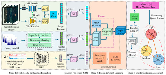
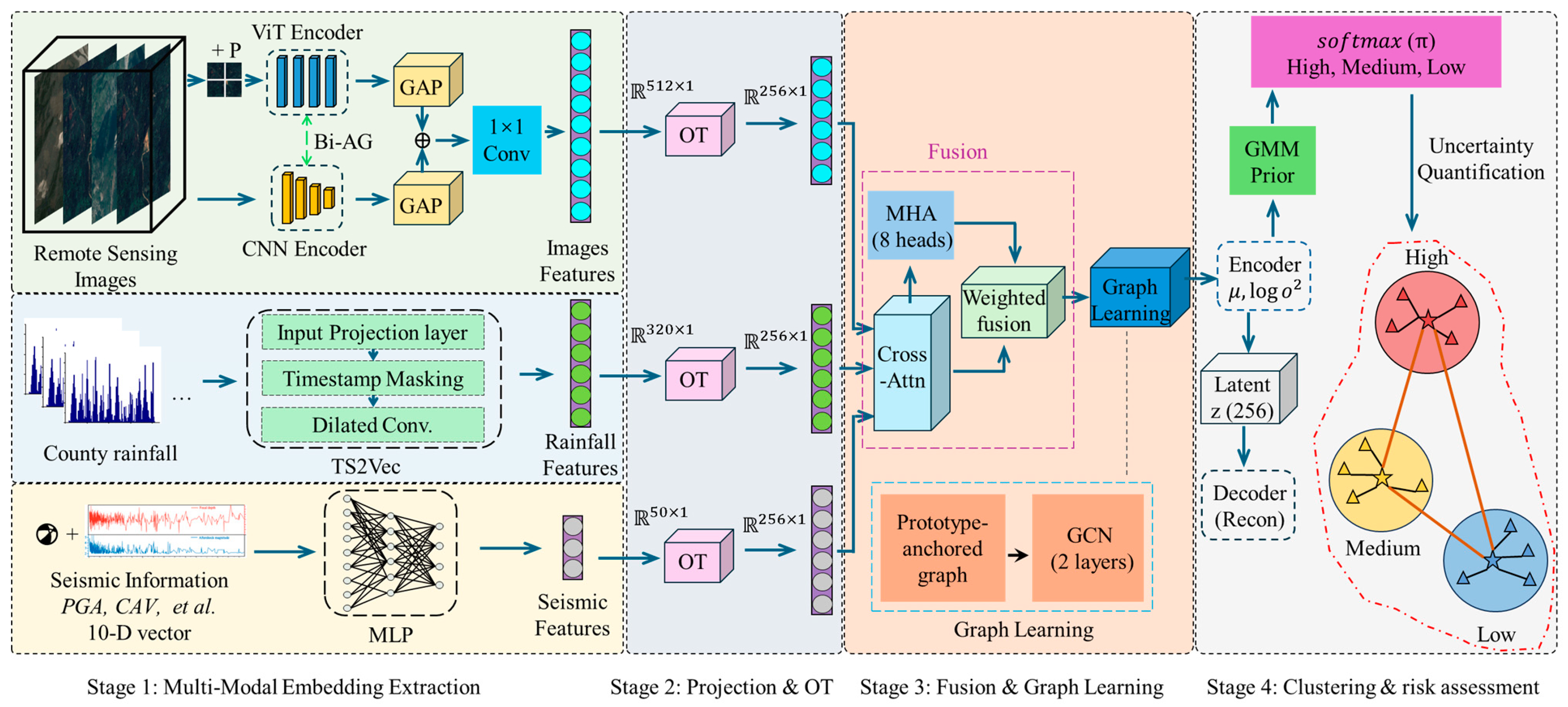
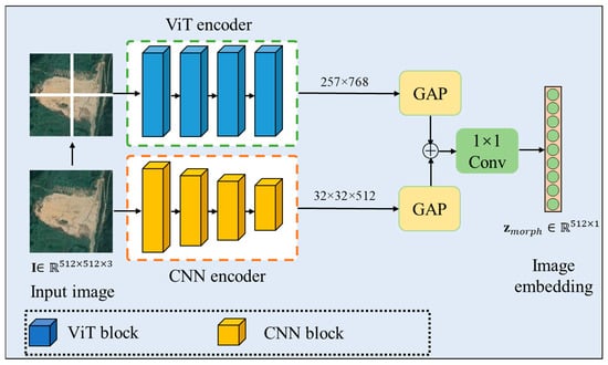
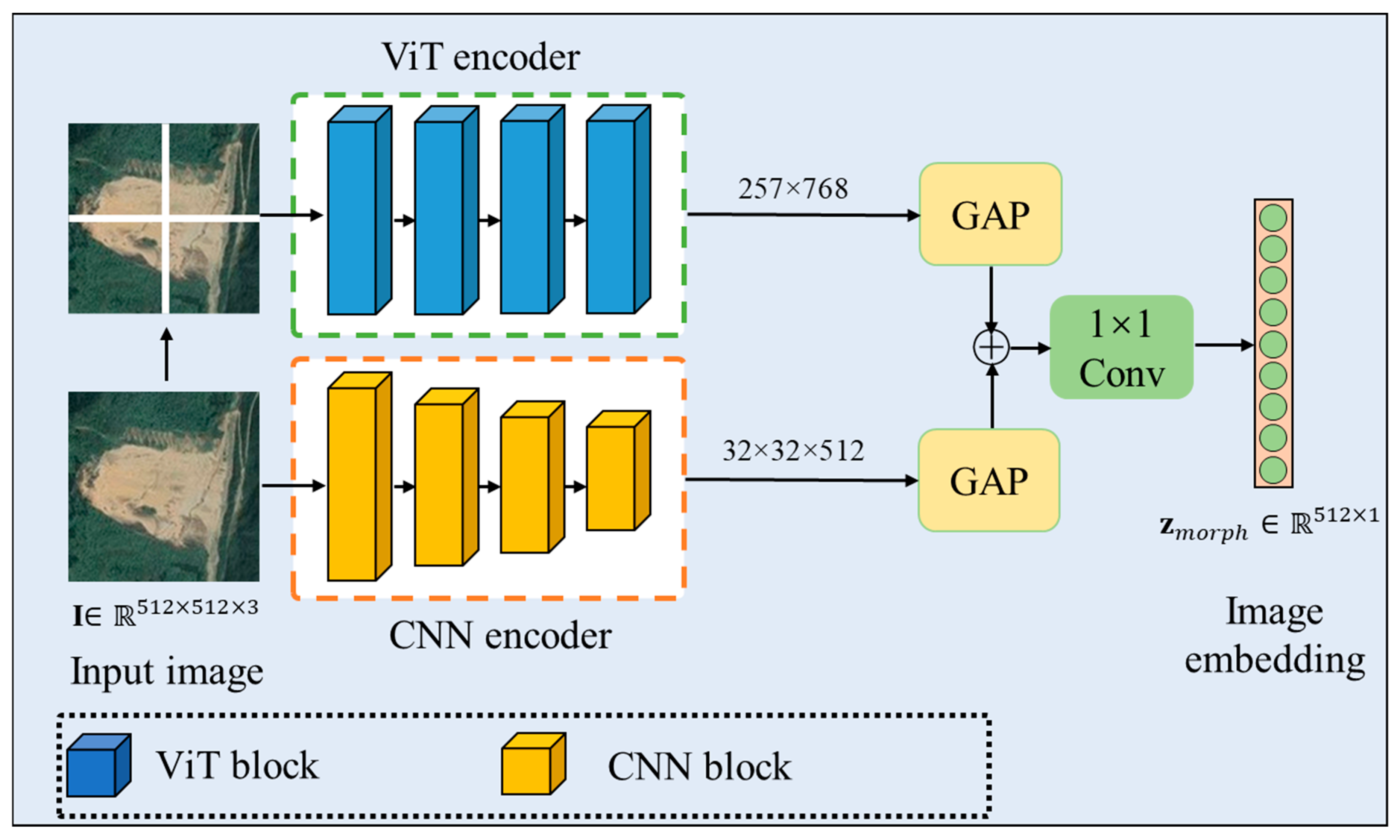
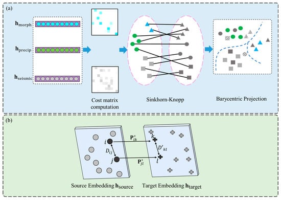
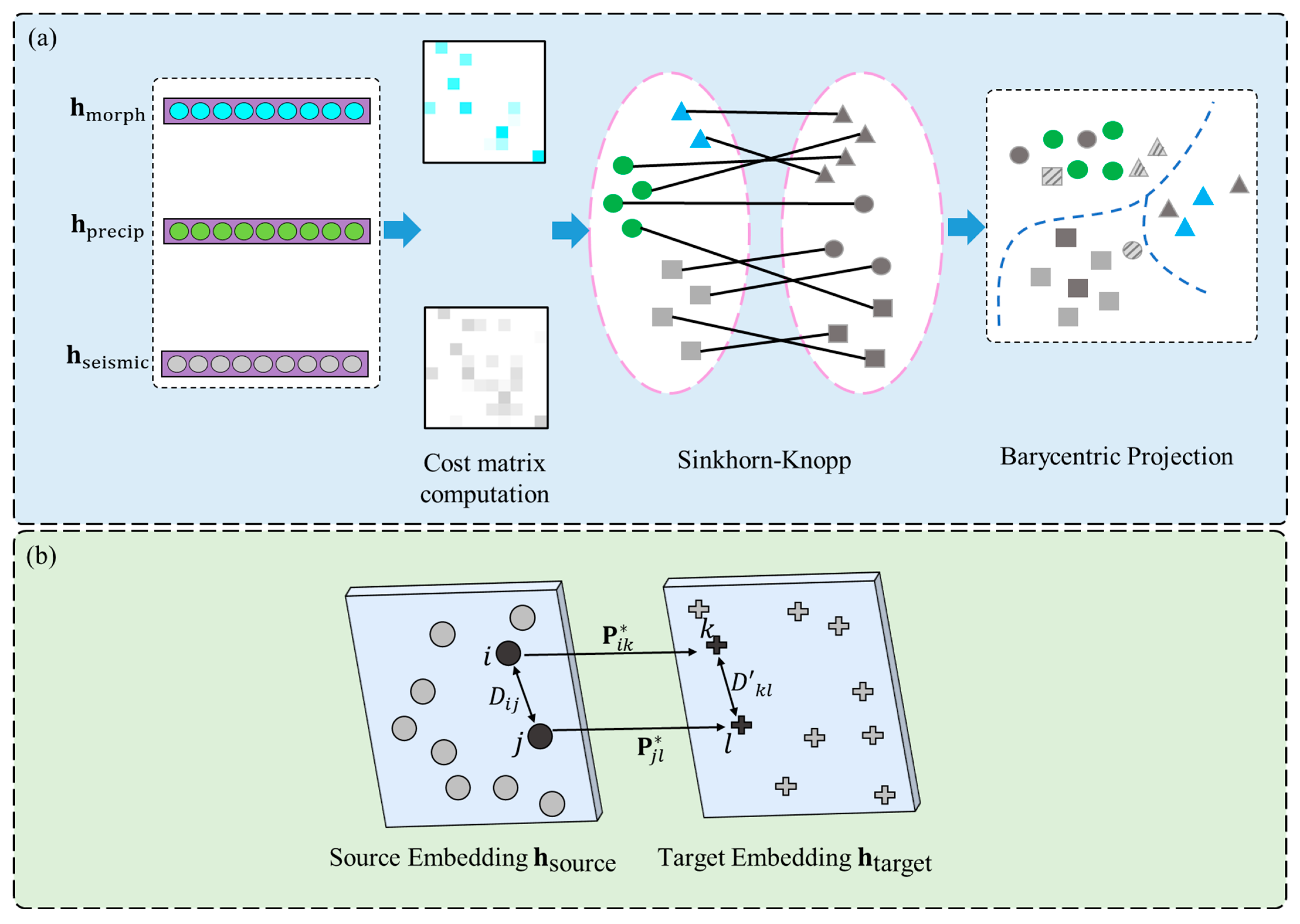
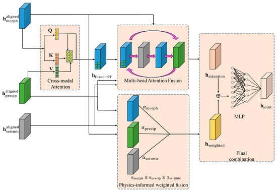
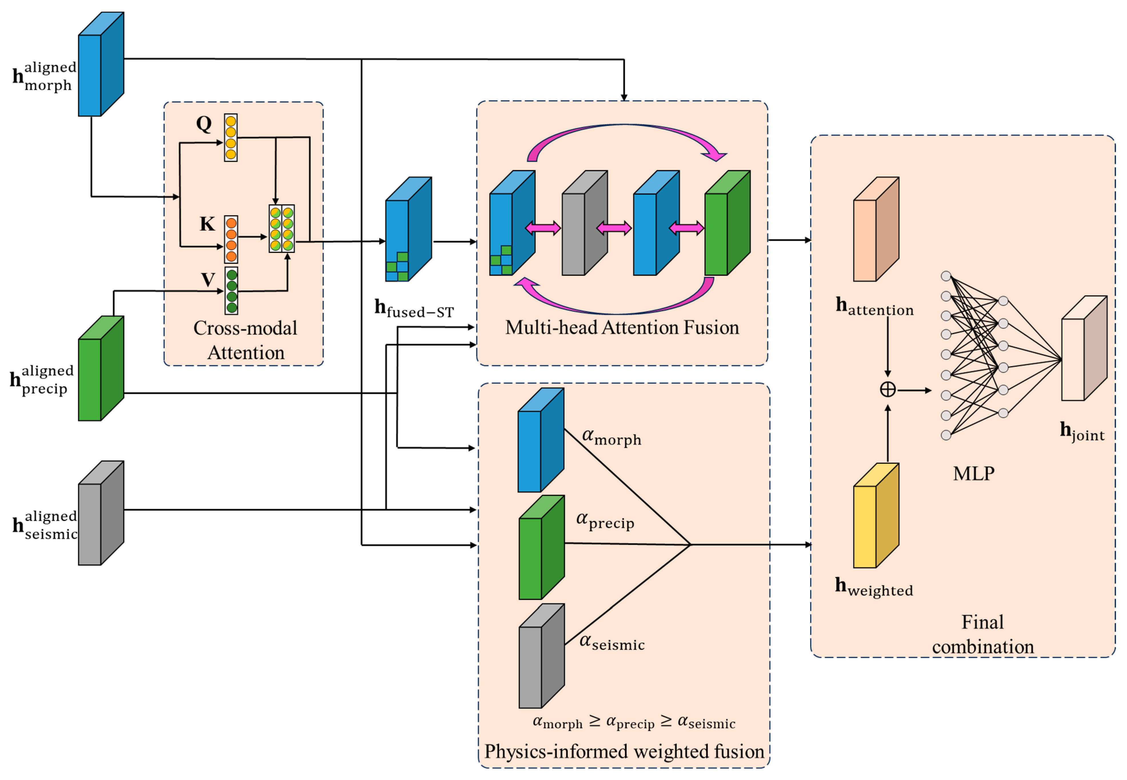
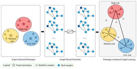
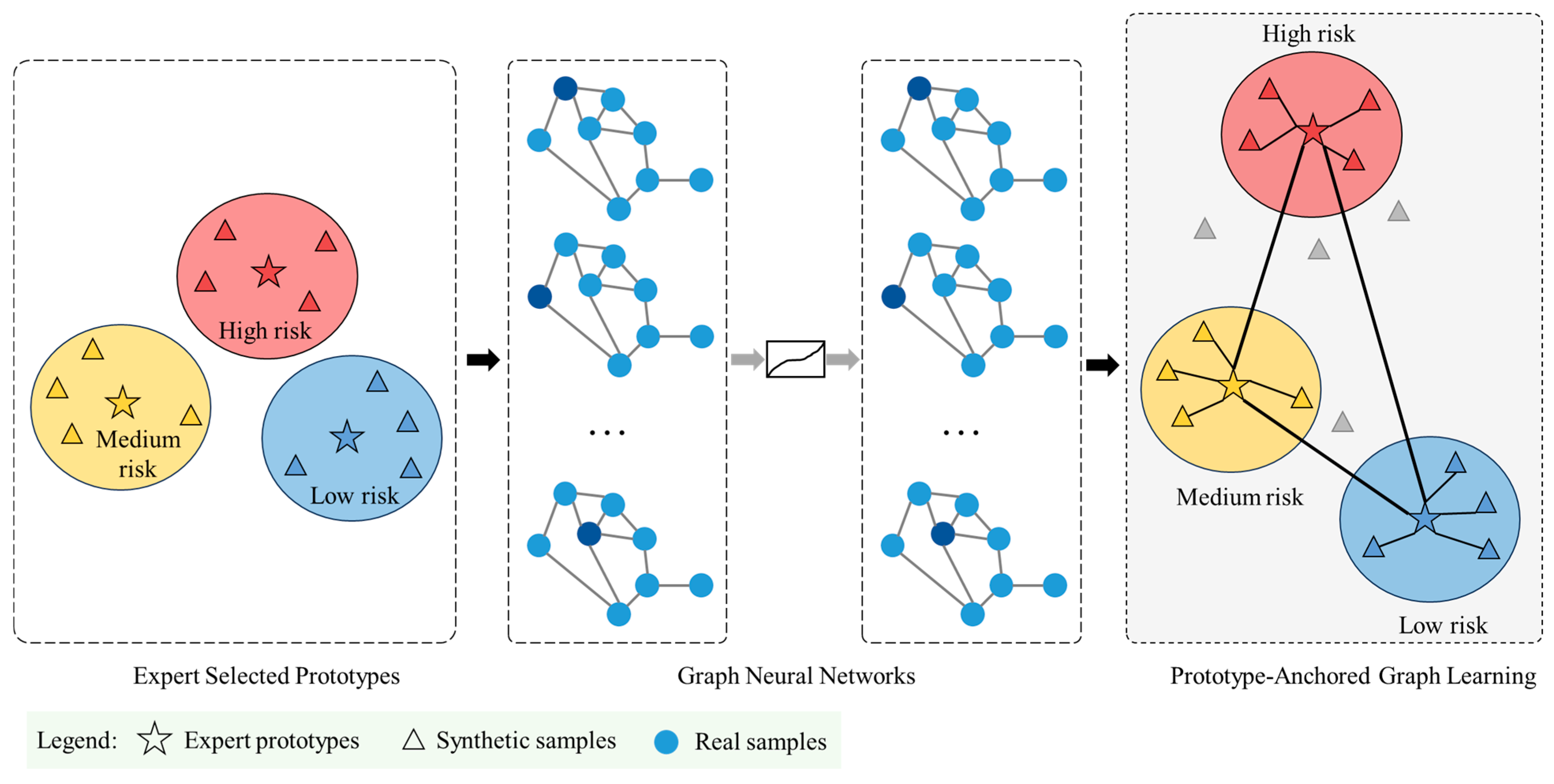
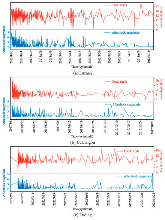
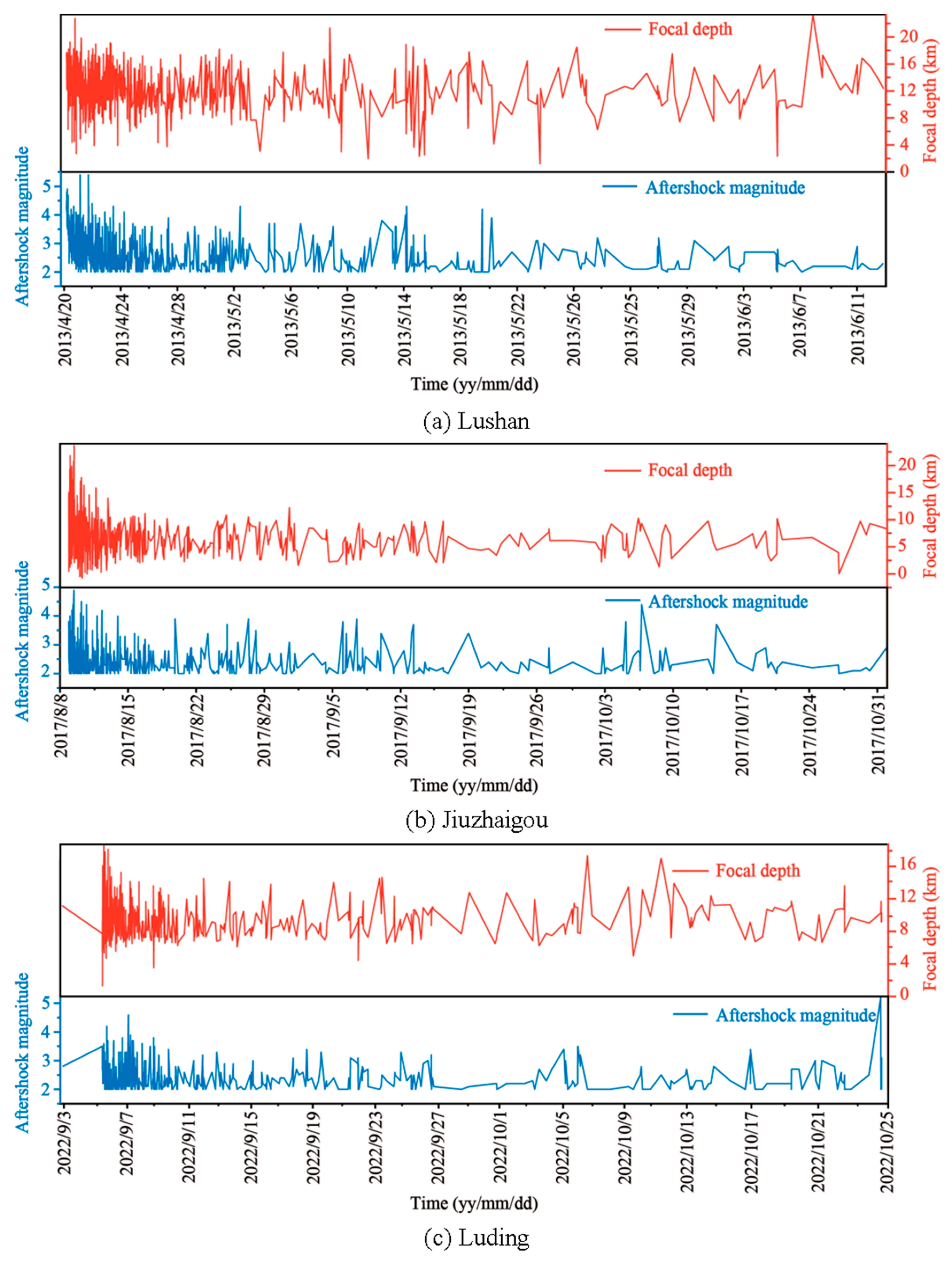
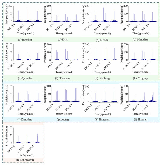
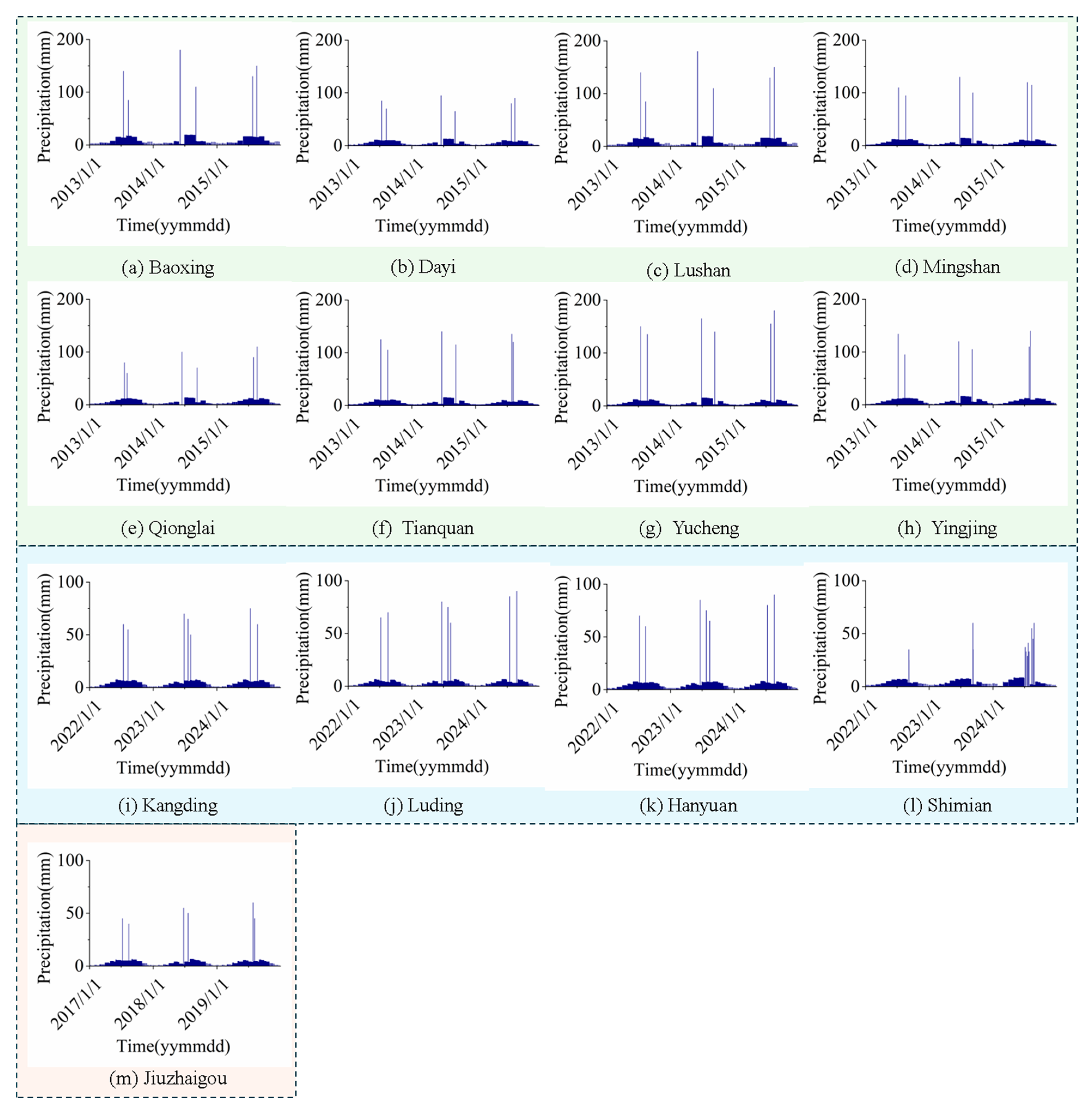
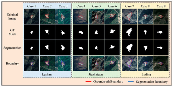
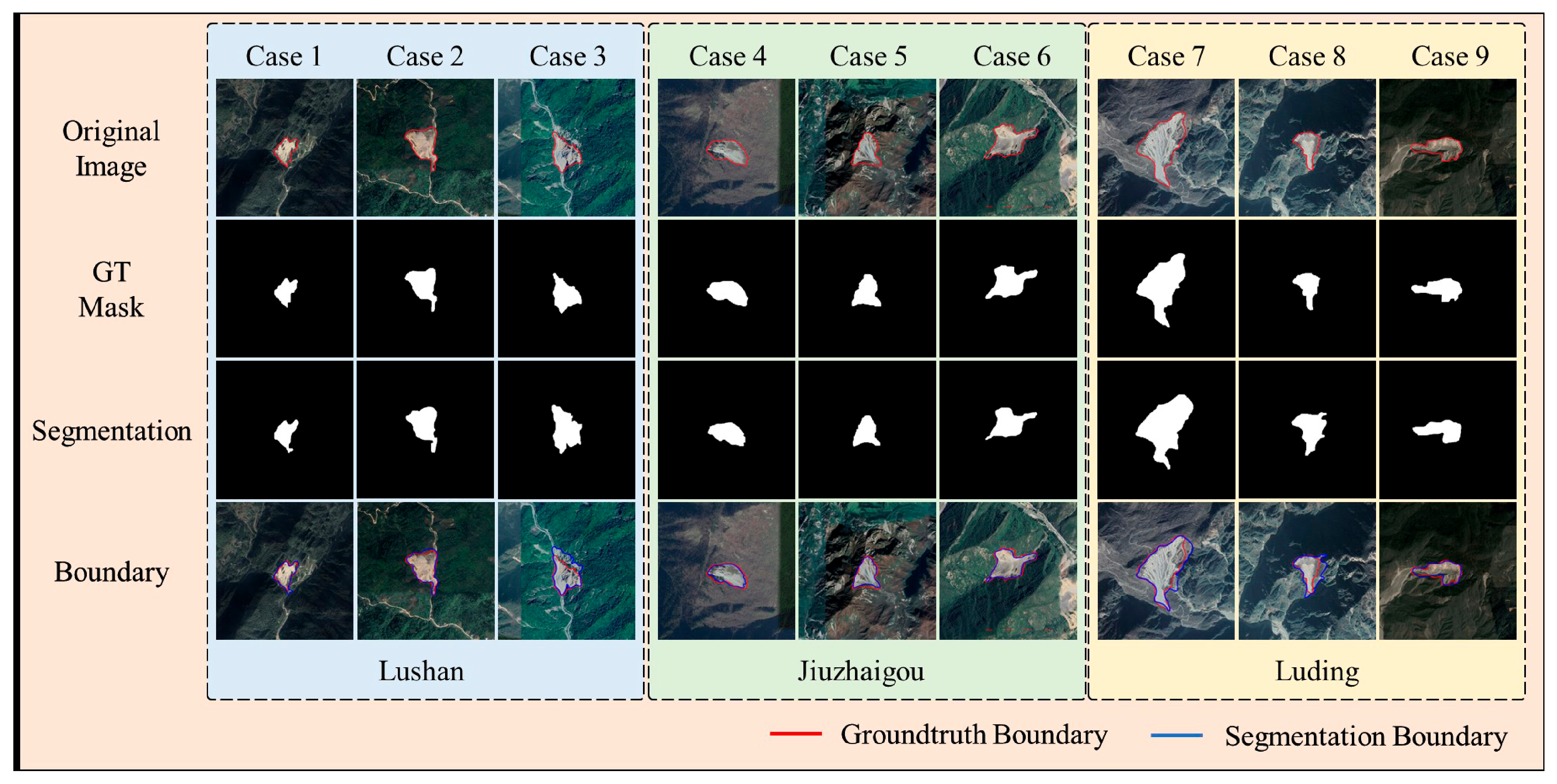
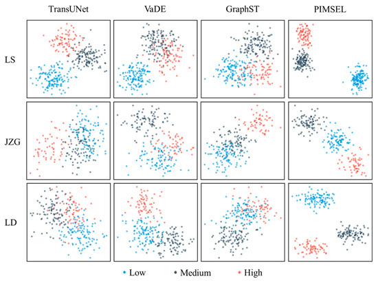
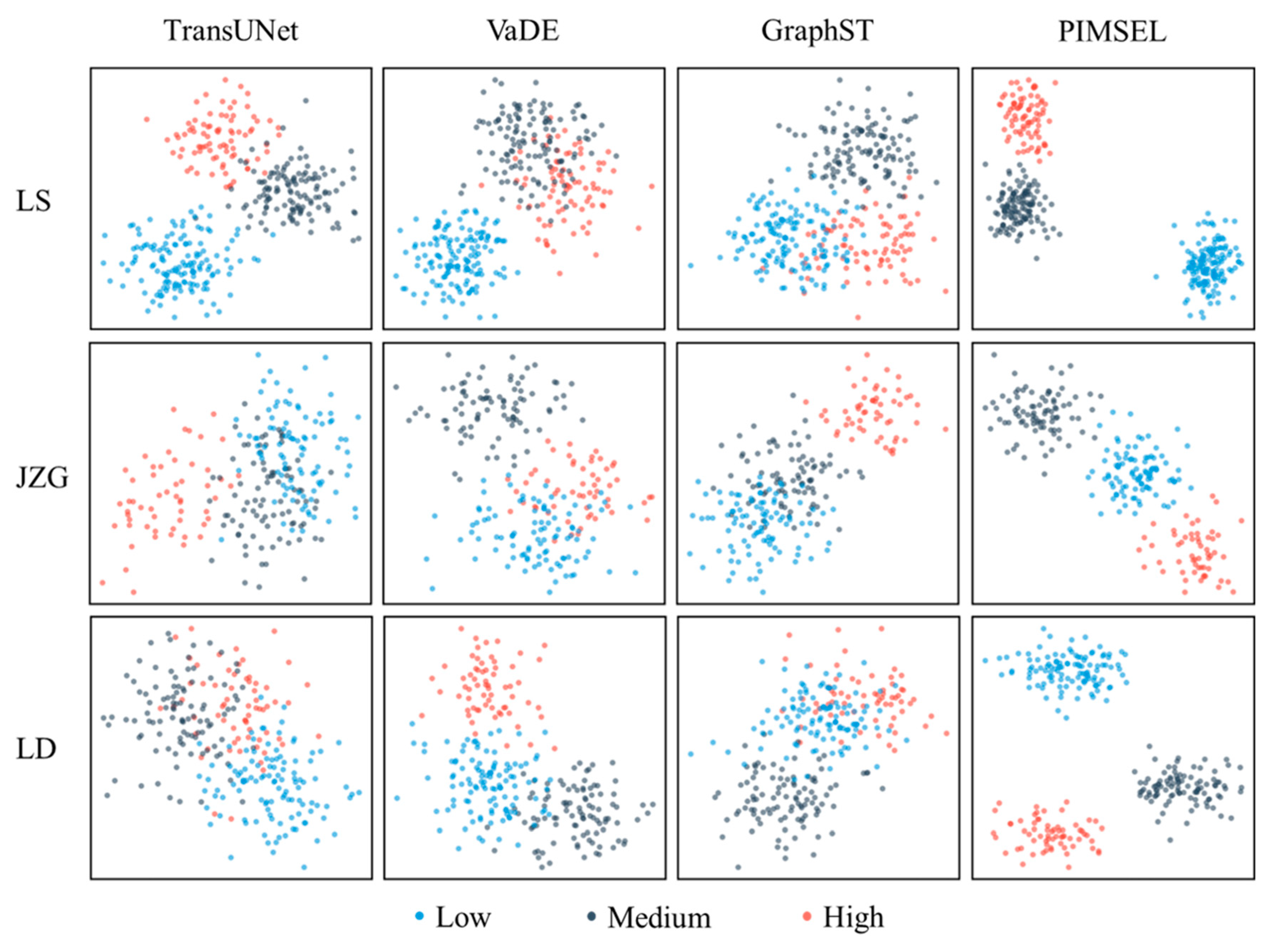
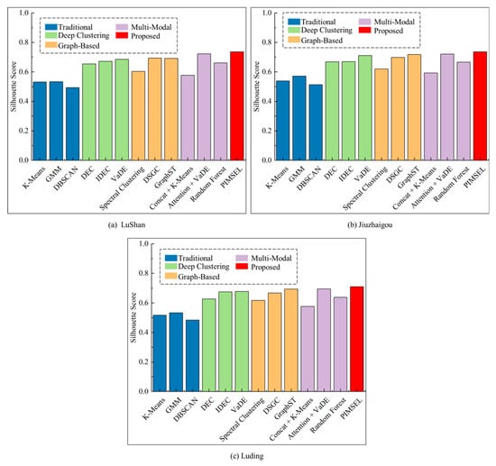
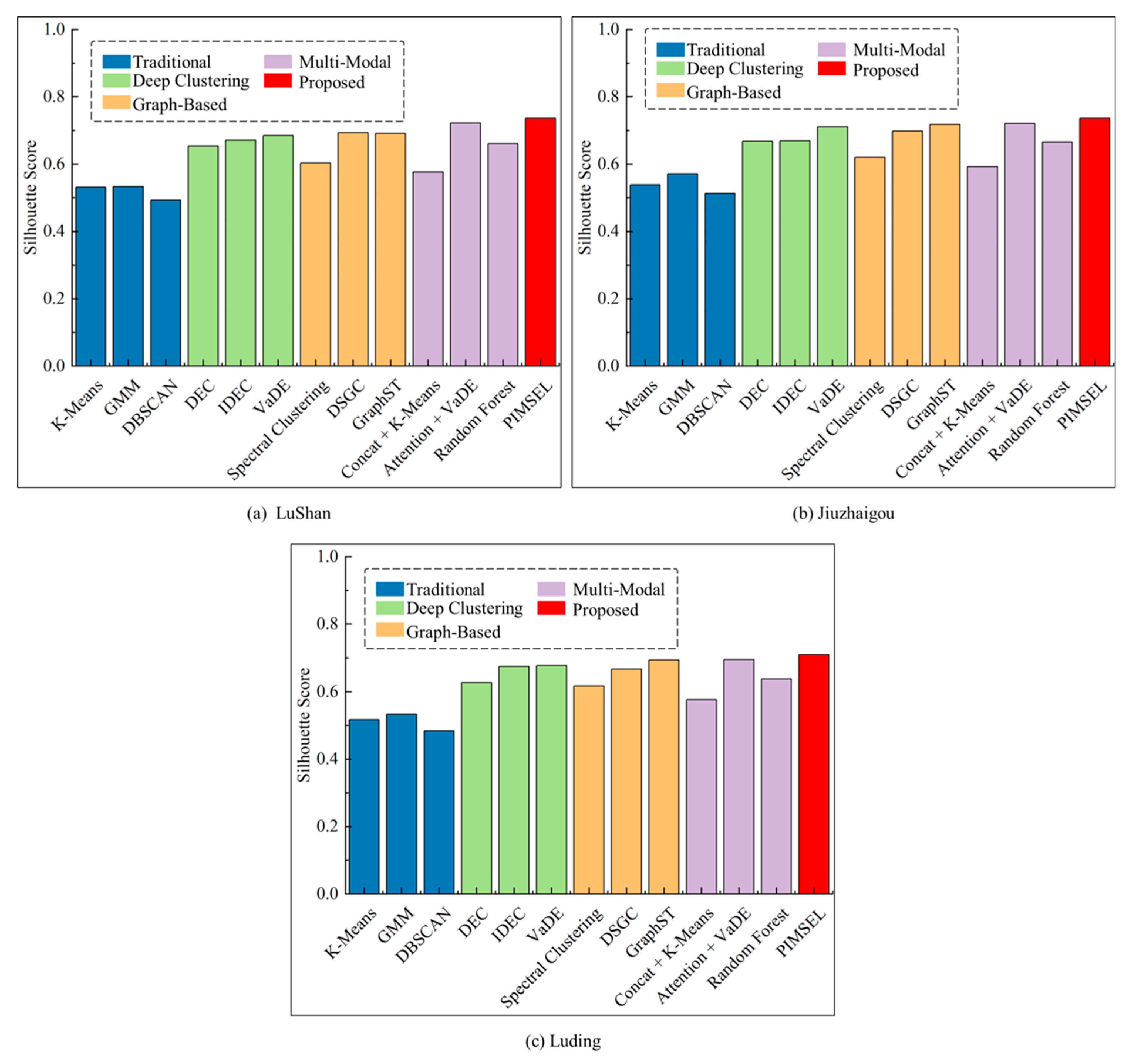
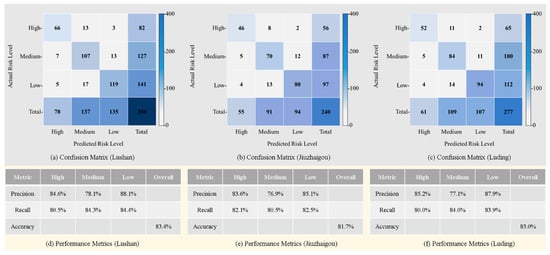
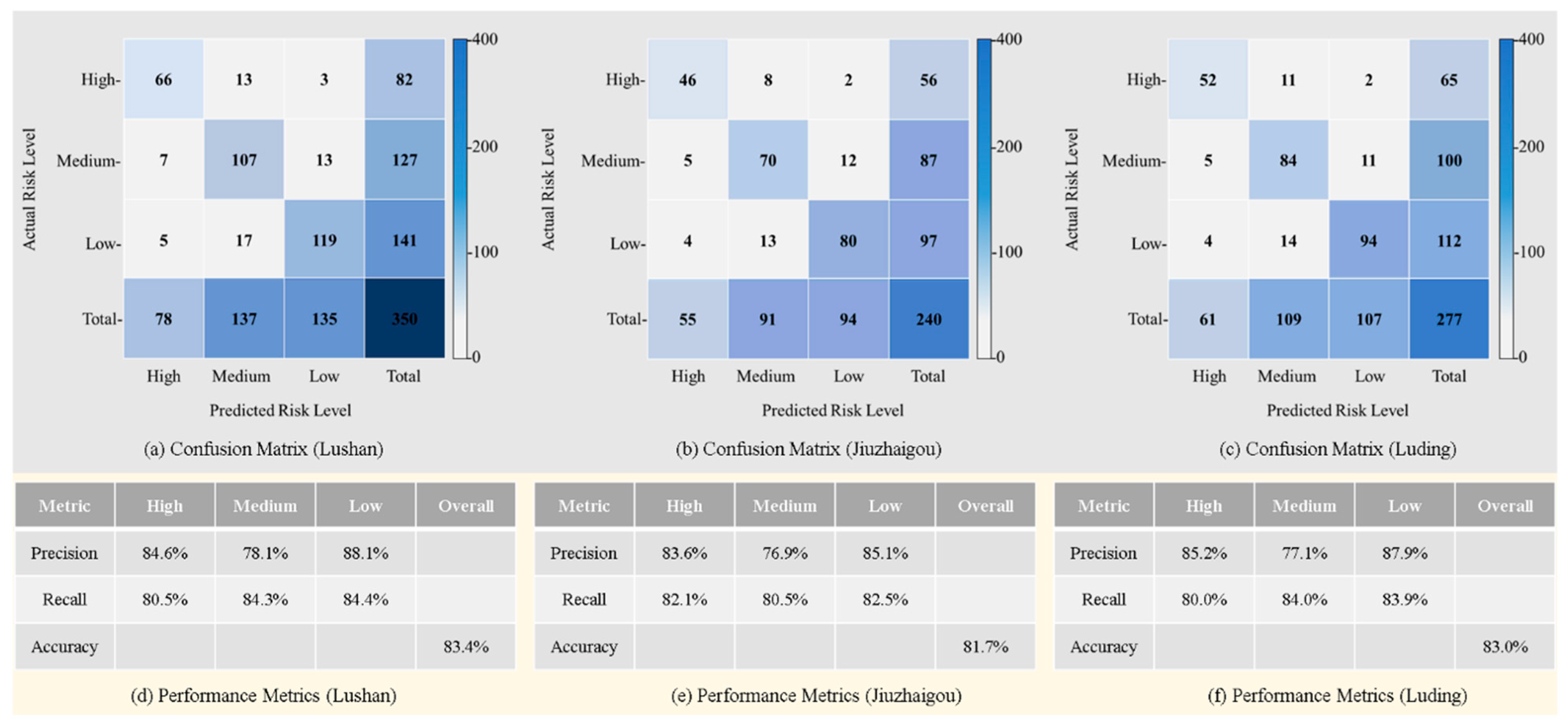
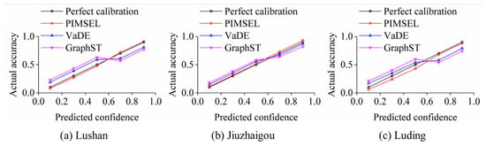
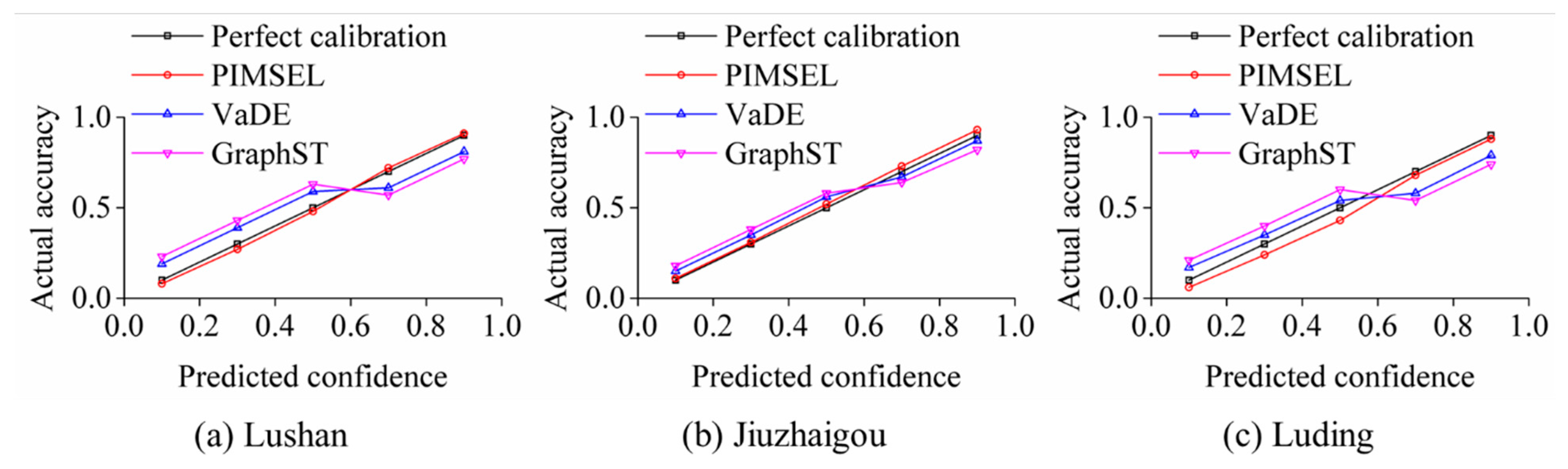
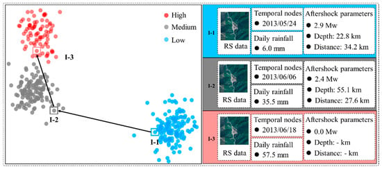
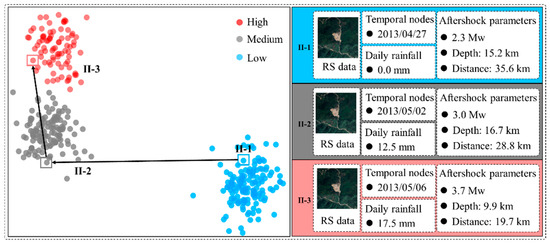
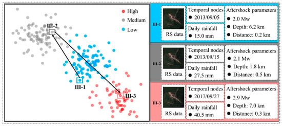
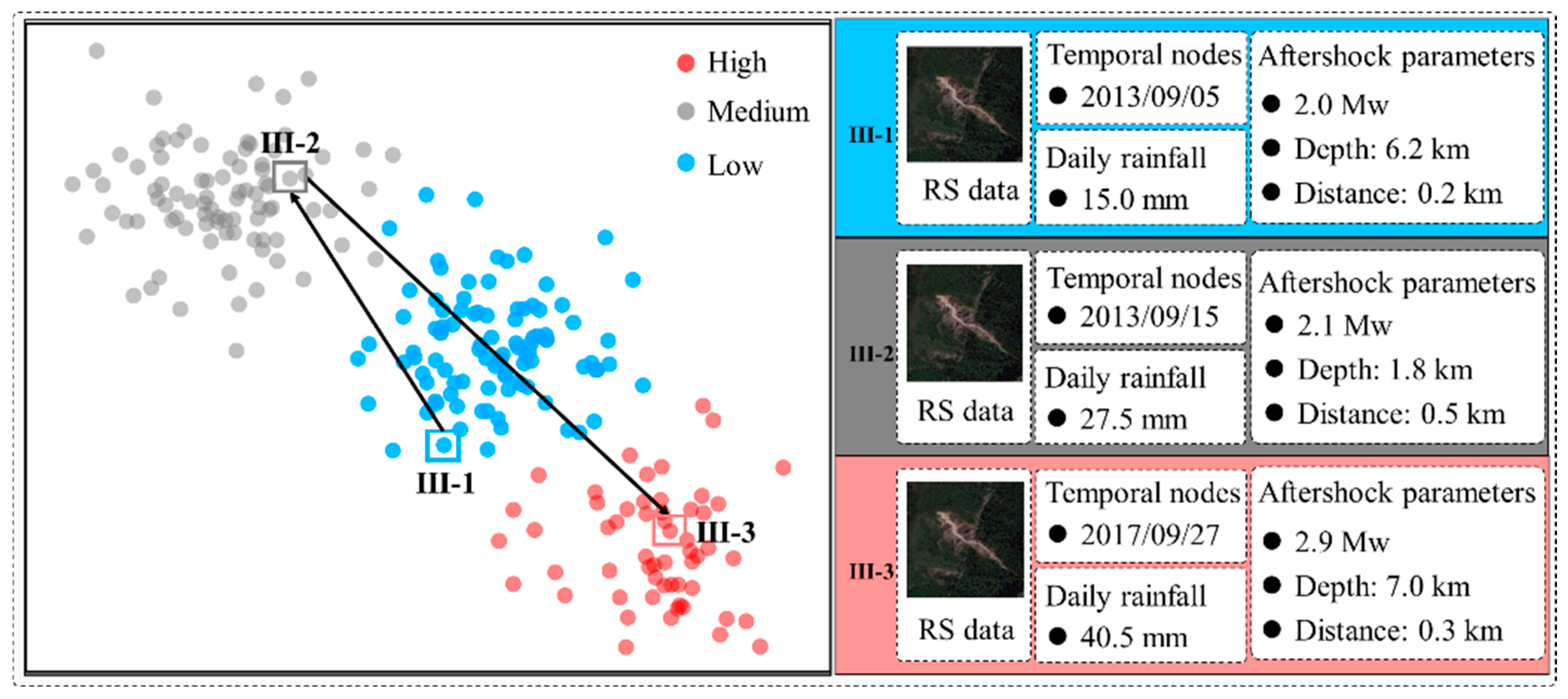
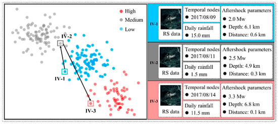
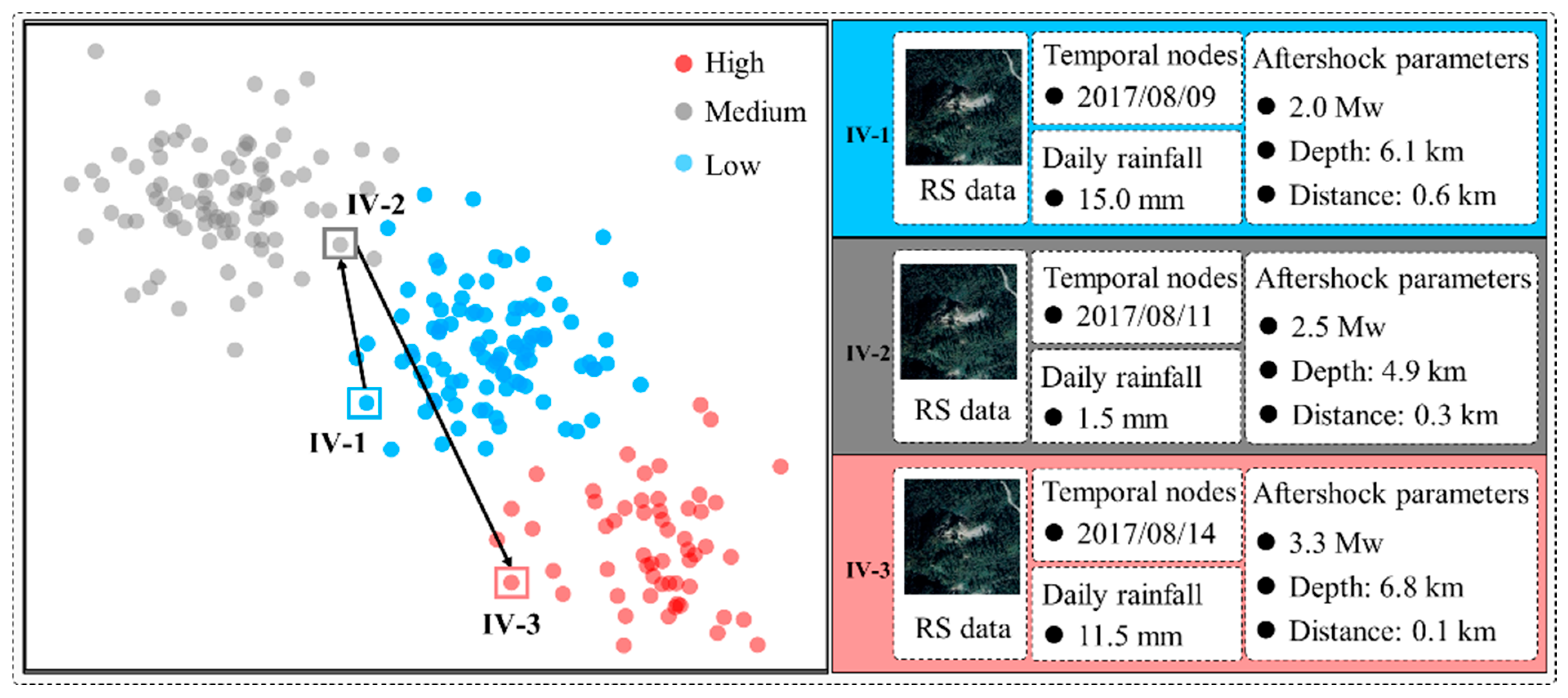
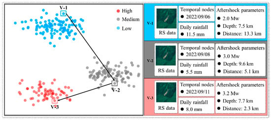
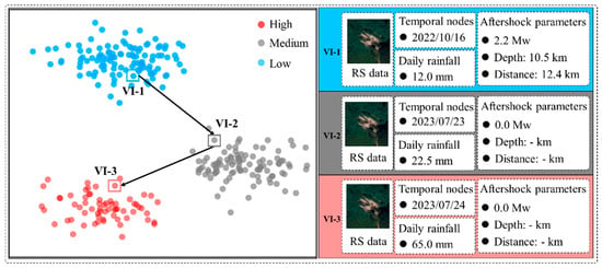
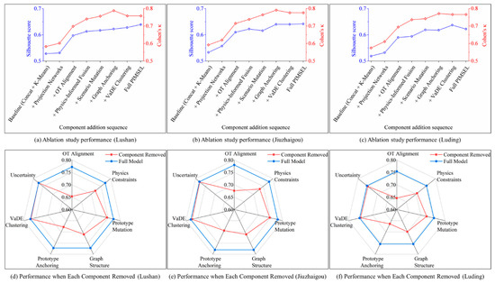
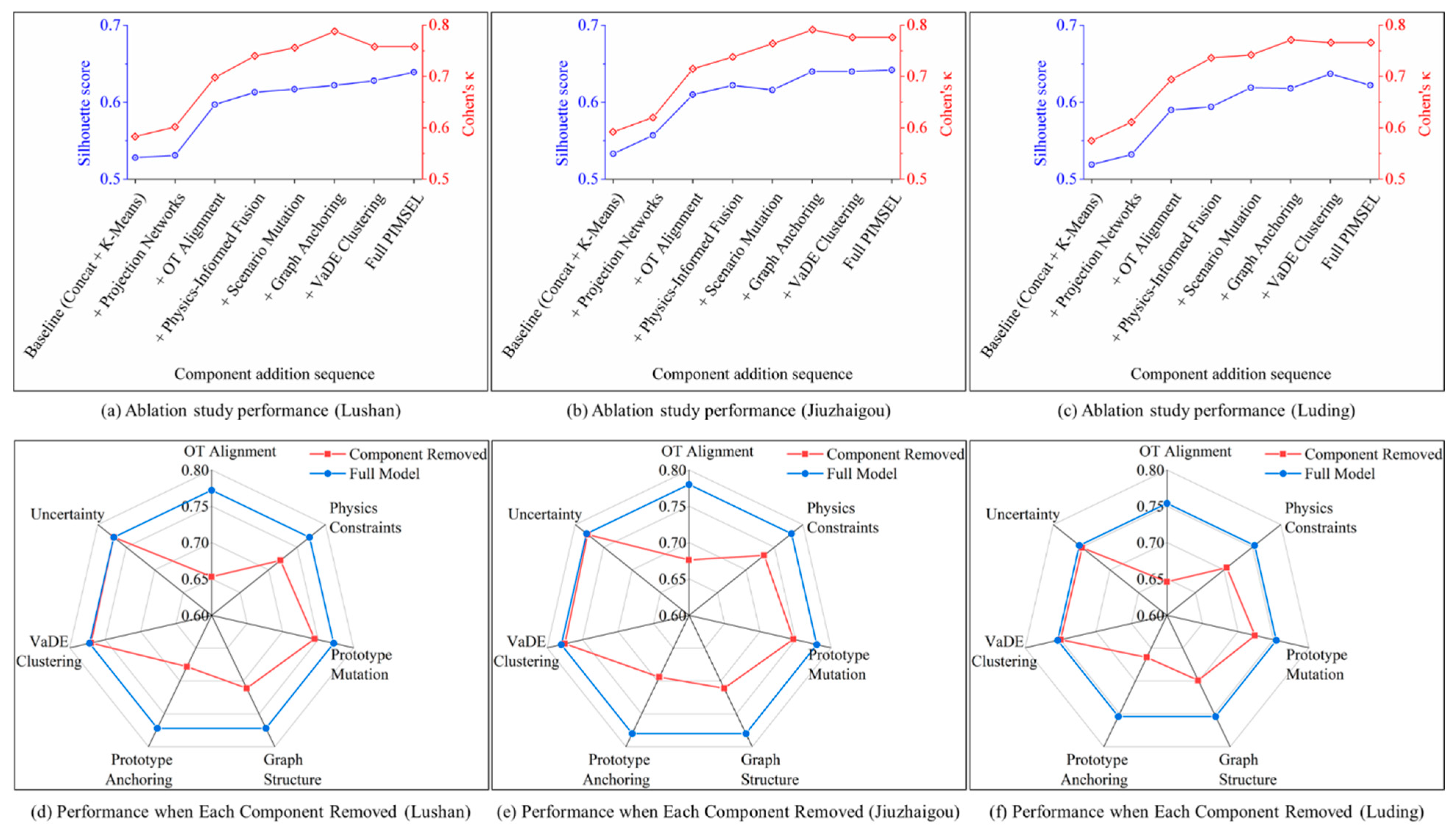

Disclaimer/Publisher’s Note: The statements, opinions and data contained in all publications are solely those of the individual author(s) and contributor(s) and not of MDPI and/or the editor(s). MDPI and/or the editor(s) disclaim responsibility for any injury to people or property resulting from any ideas, methods, instructions or products referred to in the content. |
© 2026 by the authors. Licensee MDPI, Basel, Switzerland. This article is an open access article distributed under the terms and conditions of the Creative Commons Attribution (CC BY) license.