


Highlights
What are the main findings?
- We developed the LandCycler algorithm, a novel time-series approach that integrates median-based, probability-based, and number-based models to detect shifting cultivation cycles and fallow periods from Landsat time series (1988–2020) with robust performance (producer’s accuracy: 82.12%; user’s accuracy: 81.37%).
- Shifting cultivation covers 16.79 × 10⁴ km2 across Southeast Asia (affecting ~10% of regional forests), with an average of two cultivation cycles and 10 years fallow period; over 98% of shifting cultivation areas experienced four or fewer deforestation events during the study period.
What are the implications of the main findings?
- Precise detection of shifting cultivation cycles and fallow periods enables evidence-based assessment of forest disturbance regimes, providing critical data for evaluating whether fallow period lengths are sufficient to maintain soil fertility, support biodiversity recovery, and sustain ecosystem services, key factors distinguishing sustainable traditional practice from degrading land use intensification.
- The LandCycler algorithm provides a transferable, large-scale mapping tool that enables accurate quantification of shifting cultivation dynamics, filling a critical gap for sustainable agroforestry management, REDD+ policy implementation, and forest conservation planning in tropical regions.
Abstract
Shifting cultivation (SC) is a predominant land use across the tropics, feeding hundreds of millions of marginalized people, causing significant deforestation in tropical regions. A key question is how to realize rapid and large-scale identification of the spatial distribution, cycle numbers, and fallow periods of SC. Building the LandCycler algorithm that fully considers the inter-annual cycle of SC based on Landsat imagery from 1988 to 2020, we identify the distribution and fallow period of SC in Southeast Asia, including Assam in India and Yunnan Province in China. The results show that the LandCycler for the identification of SC is satisfactory (producer’s accuracy 82.12% and user’s accuracy 81.37%), and the accuracy in detecting the average cycle number, and calculating the average fallow period is 83.71%, and 96%, respectively. We found that the total area of SC is as high as 16.79 × 10⁴ km2 in Southeast Asia, which uses almost 10% of the total forests. Meanwhile, the average cycle number and the average fallow period of SC are two times and 10 years, respectively. More than 98% of SC has repeated deforestation four times or less. The shorter the distance from settlements and the distance from roads, the larger the cycle number of SC. Although there was no significant correlation between elevation and slope and the cycle number of SC, SCs were mainly distributed at slopes of 18 ± 5° and elevations of 800 ± 300 m. These findings provide effective tools for sustainable agroforestry management as well as for global SC mapping.
1. Introduction
Shifting cultivation (SC), also known as swidden agriculture or slash-and-burn farming, is one of the oldest and most widespread land use practices in the tropical regions [1]. It is estimated that SC supports the livelihoods of 200–300 million marginalized people across the tropics, particularly in Southeast Asia, Africa, and the Amazon basin [2,3]. As a cyclical land use system, SC involves the clearing of forest patches, cultivation of crops for one to three years, and subsequent abandonment to allow natural vegetation regrowth during a fallow period [1]. When properly managed with an adequate fallow period, an SC can maintain soil fertility, support biodiversity, and provide ecosystem services [4]. However, increasing population pressure, land use policies, and market integration have accelerated the intensification of SC, leading to shortened fallow periods, expanded deforestation, and increased forest degradation [5].
Southeast Asia is a global hotspot of tropical deforestation and land use change [6], where SC remains a predominant farming system in the mountainous regions [7]. The Montane Mainland Southeast Asia (MMSEA), including parts of Myanmar, Laos, Vietnam, Thailand, and adjacent areas of China and India, has been identified as one of the most active SC regions worldwide [3,8,9]. Despite its ecological and socioeconomic significance, the precise spatial distribution, intensity, and dynamics of SC in this region remain poorly quantified. Traditional assessments of SC have largely relied on field surveys [10], expert interviews [11], or coarse-resolution maps, which are insufficient for capturing the fine-scale patch dynamics and temporal cycles characteristic of SC systems. The lack of spatially explicit, high-resolution, and temporally consistent SC maps hinders our ability to assess its environmental impacts, support sustainable land use planning, and inform policy interventions such as the implementation of Reducing Emissions from Deforestation and Degradation (REDD+) [12].
Remote sensing offers a promising avenue for large-scale SC mapping. The opening of the Landsat archive and the development of cloud computing platforms such as Google Earth Engine (GEE) have enabled wall-to-wall, time-series analysis of land surface dynamics at 30 m resolution [13]. Several algorithms have been developed to detect forest disturbance and recovery using the Landsat time series, such as LandTrendr [14] and continuous change detection and classification (CCDC) [15]. However, these algorithms are primarily designed for generic forest change detection and are not optimized for capturing the cyclical forest–cropland–forest transitions characteristic of SC. Specifically, SC-identification requires not only detecting deforestation events, but also quantifying the number of cultivation cycles and the length of fallow periods—key parameters that determine the sustainability and environmental impact of SC systems [1]. Moreover, existing SC mapping efforts have been limited to local scales [16] or rely on visual interpretation [10], making them difficult to replicate consistently across large areas.
To address these gaps, we developed a novel algorithm—LandCycler (LC)—that explicitly models the inter-annual cycle of SC based on dense Landsat time series from 1988 to 2020. The LandCycler algorithm integrates three complementary pathways (median-based, probability-based, and number-based models) to robustly determine annual land use states and detect cyclical forest–cropland–forest transitions. It further incorporates spike removal, change point detection, and fallow period calculation to characterize the full cultivation cycle. The objectives of this study are to: (1) develop and validate the LandCycler algorithm for detecting shifting cultivation cycles and fallow periods from Landsat time series; (2) map the distribution, cycle number, and fallow period of SC across Southeast Asia (1988–2020); and (3) analyze the biophysical and socioeconomic factors influencing SC spatial patterns. Our results provide a foundational dataset for understanding the role of SC in regional land use dynamics and offer a transferable tool for global SC mapping in other tropical regions.
2. Materials and Methods
2.1. Study Area
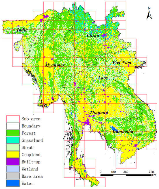
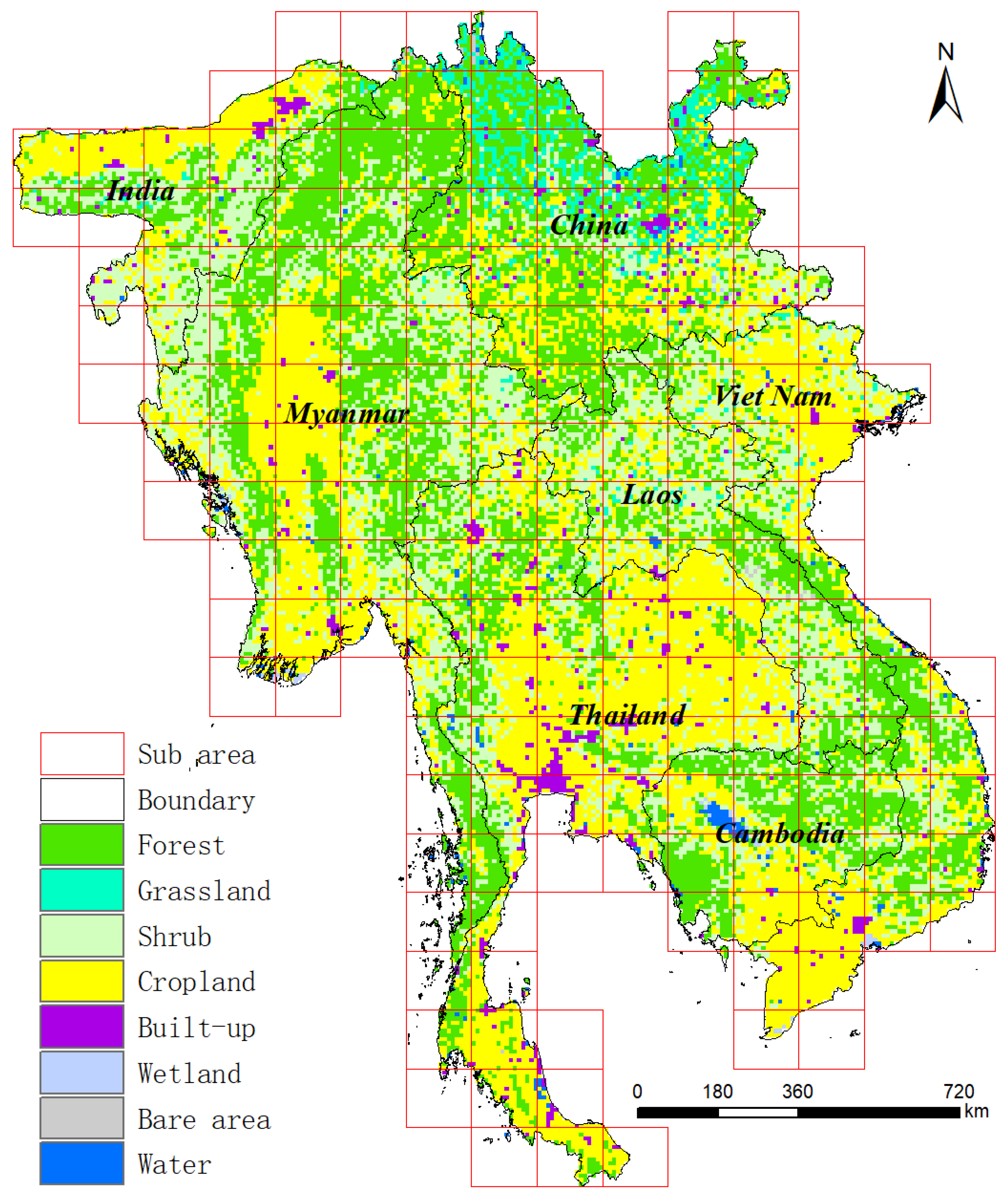
In this study, all mainland countries throughout Southeast Asia and the adjacent provinces of China and India were selected as the study area (Figure 1). To improve computational efficiency, we divided the study area into 178 small sub-study areas. Except for crops and plantations, the vegetation is mainly tropical evergreen forest [6,17]. As an active area of land use change, Southeast Asia has become the focus area [18]. As one of the most important areas of tropical forest in the world, the main farming method here is shifting cultivation [1,7]. The Landsat image is selected as the basic data, and the research period is set to 1988–2020.
Figure 1.
Study area. The base map is a 1 km resolution land cover data from 2010, used to macroscopically display the basic characteristics of the study area. The blocks in the figure are divided into 178 sub regions.
2.2. Study Framework
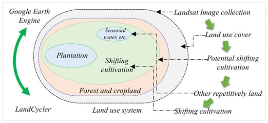
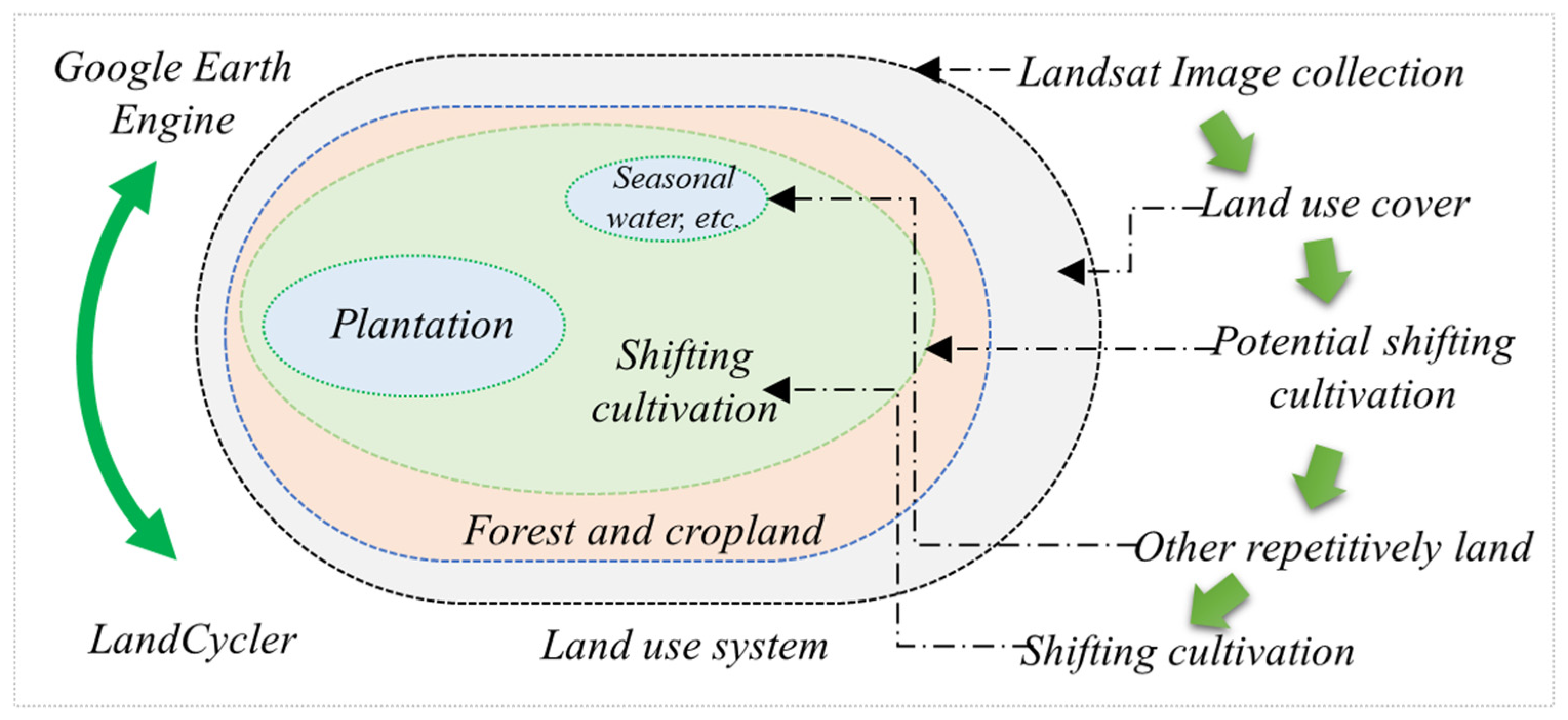
Based on the GEE platform, this paper builds an LC algorithm for detecting dynamic changes in pixels (Figure 2). Identify potential SC areas by detecting pixels with repetitive disturbance characteristics (forest–cropland–forest–cropland). Furthermore, we further identified and removed other repetitive disturbance lands (repetitive waters, plantations, etc.) that do not belong to SC. The intra-annual and inter-annual variations in spectral information and the radar information of land types provide the basis to identify and remove non-SC pixels. Finally, we completed a mapping of SC which included the cycle number, and average fallow period over the study period. The spatial resolution of all maps is 30 m. The data used in this study are the Landsat Collection 1 Level-1 products, Sentinel 1 dataset, ESA WorldCover products [19], and Joint Research Centre’s Global Surface Water products from [20] GEE.
Figure 2.
Study framework for SC based on spatiotemporal relationships.
2.3. Technical Framework of LandCycler
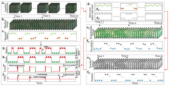
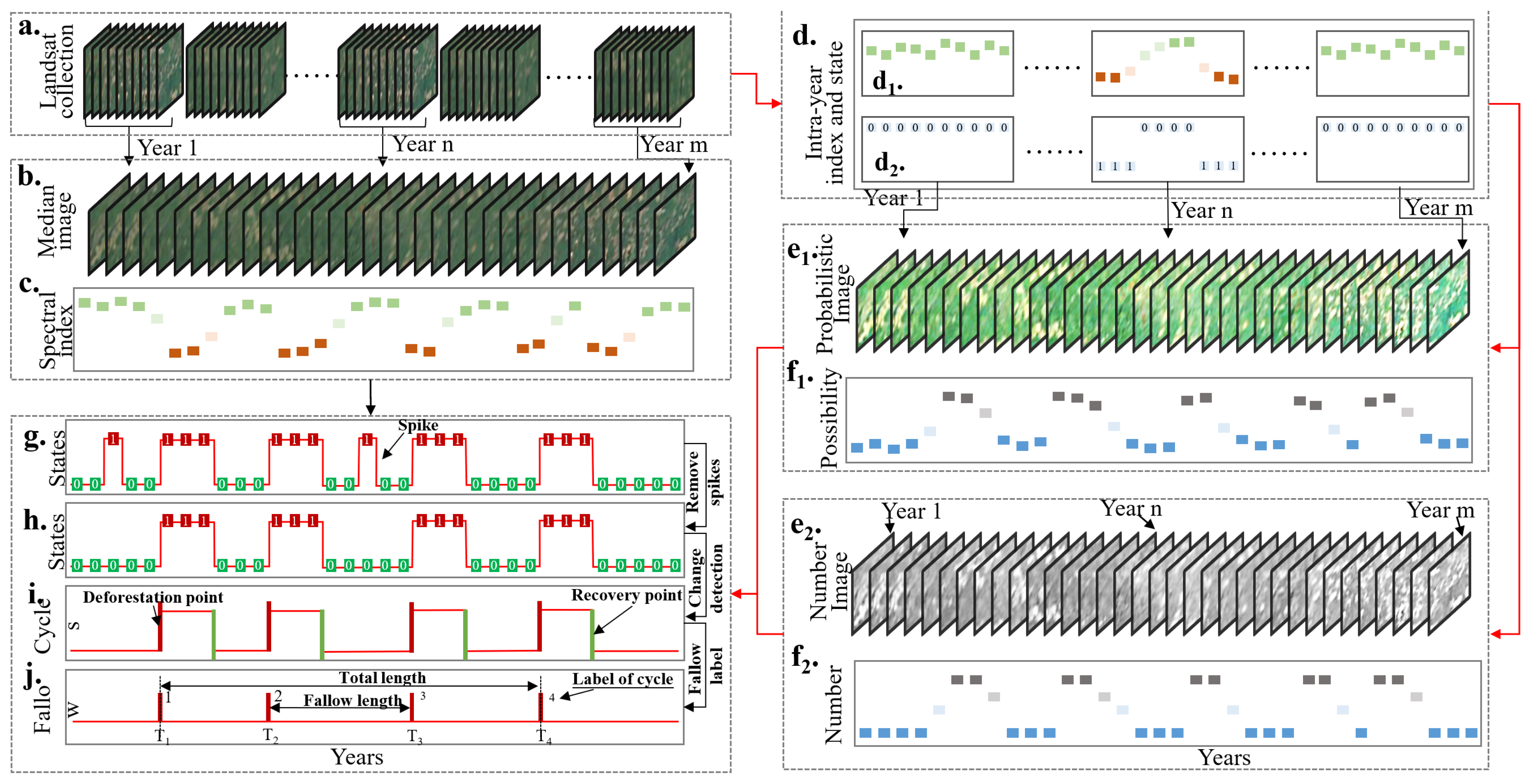
The processing flow of LC mainly includes preprocessing, index calculation, land use states determination, and cycle identification (Figure 3). Through the preprocessing process of image selection, geometric correction, noise removal, etc., the Landsat collection including all intra-year images is prepared (Figure 3a). These data were used respectively in the median model (LCm, Figure 3a–c), probabilistic model (LCp, Figure 3a,d,e1,f1) and number model (LCn, Figure 3a,d,e2,f2) to determine yearly land use states. The median model directly fuses the intra-year images into the yearly composition (Figure 3b) and then calculates the yearly spectral index (Figure 3c). Combined with dichotomy, the LC algorithm determines yearly land use states based on thresholds. The determination process of the threshold of fractional vegetation cover (FVC) is in the following (2.3.2 Threshold determination of FVC). The probabilistic model determined the yearly probability image (probability that the pixel belongs to a cropland) of the land use state (Figure 3e1) according to the intra-year land use states (Figure 3d) and then calculated the yearly probability index (Figure 3f1). Meanwhile, the number model determined the yearly number image (maximum number of consecutive low vegetation) of the land use state (Figure 3e2) and then calculated the yearly number index (Figure 3f2). Finally, based on the change state detection, LC identified and counted the cycle numbers (one process from deforestation to the nearest revegetation.) and the average fallow period length in the study period (Figure 3g–j). According to the accuracy and error characteristics of the identification results of the three models, we use the combination of their advantages to obtain the adjusted mapping results (see Section 2.5.2).
Figure 3.
Technical framework of LandCycler. (a) is a Landsat image collection obtained after preprocessing. (b) is a set of yearly median images fused based on intra-year images. (c) is the spectral index time series corresponding to each pixel in the median image. (d) shows the intra-year spectral index (d1) and land use states (d2) calculated from Landsat image collection. (e) is a yearly probability (e1)/number (e2) image determined by the intra-year proportion of different states. (f) is the probability (f1)/number (f2) time series corresponding to each pixel in the probability/number image. (g) is the yearly states determined based on three time series of the median index, probability, and number index. After identifying and removing ephemeral spikes (h), change state points are detected (i). This provides a clean state trace for recording cycle labels (j).
2.3.1. Image Preprocessing
Based on continuous detection of multiple SC areas in Southeast Asia, this study found that only the dry season (November to April) of the year had high image quality [21], and the SC area was the clearest. Deforestation mainly occurs before May. Harvest of SC mainly occurs from December to January. Deciduous forests in the dry season increase the difficulty of cropland identification (in Section 2.4). An area is considered SC (after removal of other land types, in Section 2.4) if there is no vegetation (or very low vegetation cover) between January and April. Therefore, we mainly acquired images every winter (1 January–30 April).
To maintain the consistency of images from different sensors, we correct the images of Landsat8 according to the linear relationship [22]. In addition, we unified the bands from different sensors including Landsat5, Landsat 7, and Landsat 8. Images acquired after the USGS opened the Landsat archive have gone through geometric correction and radiometric correction [13], and required no further processing. In addition, for Landsat Collection 1 Level-1 products, we build some masks from the Quality Assessment band to remove invalid pixels such as clouds, shadows, snow, and smoke.
2.3.2. Threshold Determination of FVC
The FVC is an important index to reflect the changes in the surface vegetation [23]. Since a large-scale field survey of land cover cannot be achieved, we use an FVC estimation method based on the NDVI [23].
There, and are the upper and lower thresholds of NDVI for 0.5% confidence interception, respectively.
There, and are the near-infrared and red bands of Landsat, respectively.
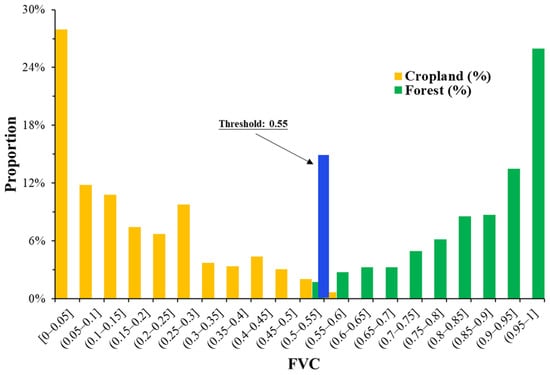
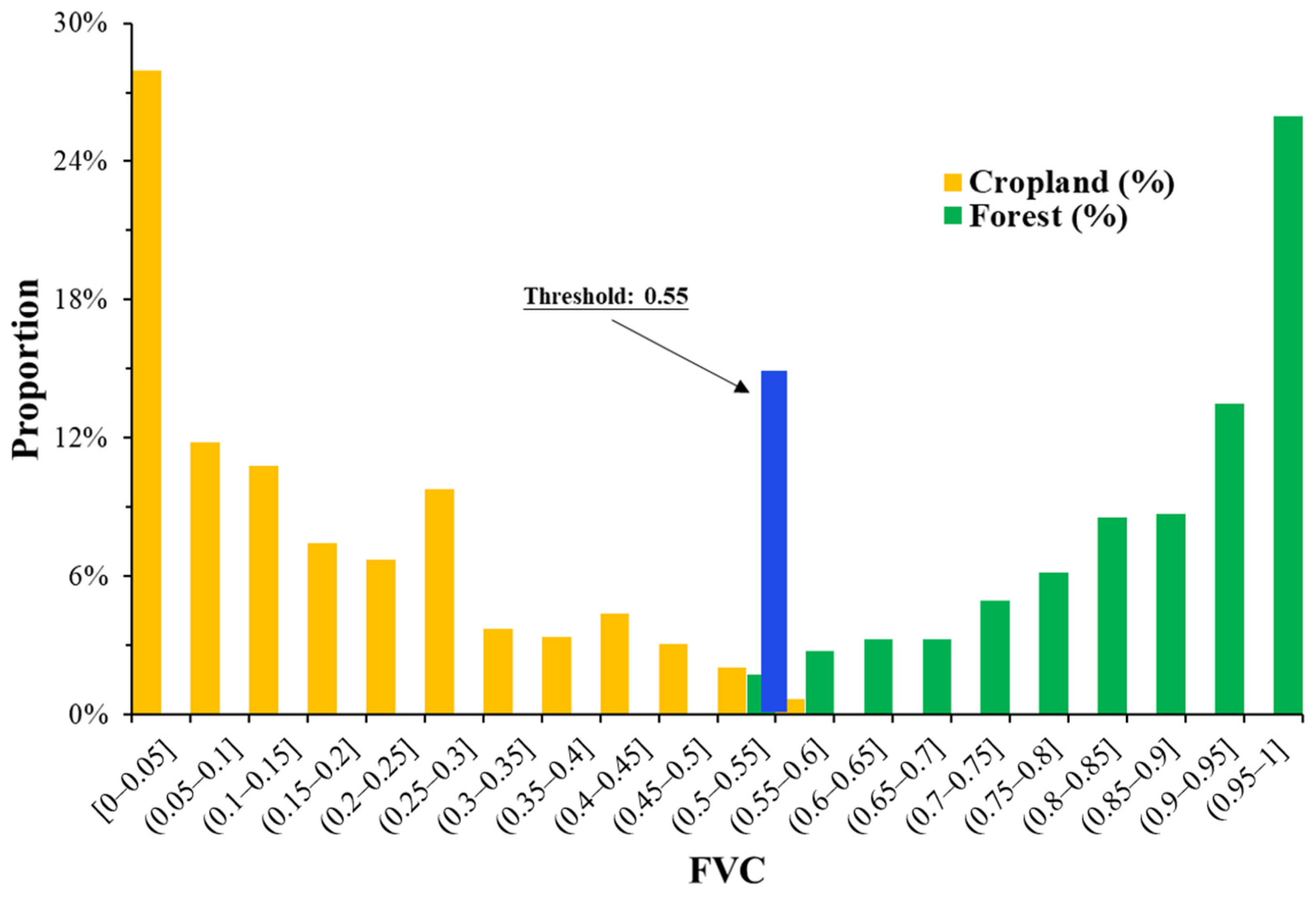
Since SC only involves the cyclical conversion of forest and cropland, we only consider these two land types when setting the threshold. For other ecosystems, the threshold can be adjusted appropriately. We generated 1000 random points in Southeast Asia to determine the FVC threshold. LC algorithm distinguishes the types of random points based on WorldCover 10 m resolution land use data [19]. Among them, 297 points belong to Cropland, and 585 points belong to Forest. According to the FVC distribution, as FVC increases, the proportion of cropland decreases rapidly. Forest is the opposite. Accordingly, we set the FVC threshold to 0.55 (Figure 4). At this value, 90.9% of cropland samples fall below the threshold and 83.8% of forest samples exceed it, providing a satisfactory separation for distinguishing active cultivation clearings from forest cover in this seasonal tropical landscape. While FVC thresholds for forest/non-forest classification vary by region and sensor, the empirical derivation of such thresholds using reference samples remains a standard and well-accepted practice in remote sensing-based land cover mapping.
Figure 4.
FVC distribution of croplands and forests. The proportion of cropland pixels before and after the threshold (0.55) is 90.9% and 9.1%, respectively. For forests, the opposite was true (16.21% and 83.78%).
2.3.3. Land Use States Determination
The LC algorithm provides three pathways, LCm, LCp, and LCn, for determining land use states. LCm uses the median model to fuse yearly high-quality images based on all intra-year images. This completely cloud-free imagery is used to calculate the FVC and further identify the land use state based on the FVC threshold. Based on the dichotomy, pixels less than the threshold are determined to be state 1. Based on all intra-year available images (after cloud removal), LCp calculates the FVC values for each image separately and identifies their land use states. The threshold used here is the same as in the median model. Then, LCp counts the number of available pixels (: the number of pixels without noise) and the number of land use state 1 () for a pixel. The probability () that this pixel belongs to state 1 is calculated (Equation (3)). Finally, LCp considers that the pixels with P1 greater than 50% belong to state 1. Meanwhile, the LCn determined the yearly maximum number of consecutive state 1. LCn assumes that the pixels that are in state 1 during more than two consecutive satellite transits belong to state 1. Finally, LCn considers that the pixel value greater than 2 belongs to state 1, and other pixels are determined to be state 0.
2.3.4. Remove Spikes
According to the causes of disturbance and recovery, there are four main reasons for the cyclical changes in land use states: natural disturbance–natural recovery, natural disturbance–human recovery, human disturbance–natural recovery, and human disturbance–human recovery. Human disturbances or recovery tend to be quicker, while natural processes are generally the opposite. For nearly 40 years, the most common types of cycles are human disturbance–natural recovery and human disturbance–human recovery. We assume that human processes, such as deforestation, can be completed within a year. Ephemeral disturbances or restorations in natural processes are considered noise-induced spurious processes (Figure 3g–h) that are defined as spikes (residual clouds and other invalid pixels) in this study [14]. For human disturbance–natural recovery, such as SC in this study area, we assumed that the spikes are ephemeral, with the land use state returning to the pre-spike state in the post-spike year, while real natural restoration of ecosystems would more persistent, with the post-spike land use state not returning to the pre-spike state quickly. If the pixel values before or after the spike are similar, the point will be removed. The default in the LC algorithm is to enable the removal of spikes.
2.3.5. Change Detection
Change state detection is the core approach we use to capture cyclical changes in land use states time series. By “change state detection”, we model a pixel’s state time series as a sequence of change points (deforestation points and recovery points, Figure 3i) that simplify the cycle features, eliminating noise but without sacrificing necessary detail. Several studies have shown that trajectory-based change detection for the first and last epochs is often unreliable because there are no images before or after the Landsat imagery in the time series [24]. Therefore, the compromise approach used in this study considers only the last year of the trajectory and not the first year. This means that deforestation that occurs in the first year is not counted, as it cannot be determined whether deforestation occurred in an earlier year.
Conceptually, a change state point in the time series is the [year, state] combination that separates a distinct land use state before it from a distinct land use state after it. The consistency of the land use states in the adjacent two years is used to judge whether the point belongs to the change state point. When the state in the observation year is inconsistent with the state in the previous year, we record the observation point as a change state point [observation year, observation state]. In addition, we divide the change state points into two categories: disturbance points and recovery points (Figure 3c). If the observation state of a changing state point is 1, the point is recorded as a disturbance point [observation year, 1]. Instead, that point is recorded as a recovery point [observation year, 0]. Detect and record the change information by pixel and by year until all observation points are detected.
2.3.6. Fallow Detection
By reading the time series of change state (in Section 2.3.5) for each pixel, the total number of deforestation (NC, number of cycles) for each pixel and the year in which each deforestation occurred were statistically analyzed. The total fallow period length (TFL) is calculated by the difference between the year of the first and the last deforestation. Finally, based on the TFL and the NC, the average fallow period length (FL) per pixel is calculated (Equation (4)).
Here, the LC algorithm does not consider incomplete cycles. For pixels with only one deforestation, the LC algorithm does not calculate the fallow period. For pixels without vegetation restoration after deforestation, LC automatically excludes them as permanent cropland or built-up area.
2.4. Remove Non-SC Land
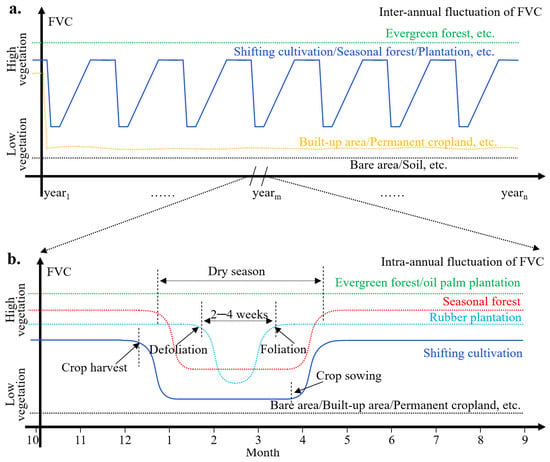
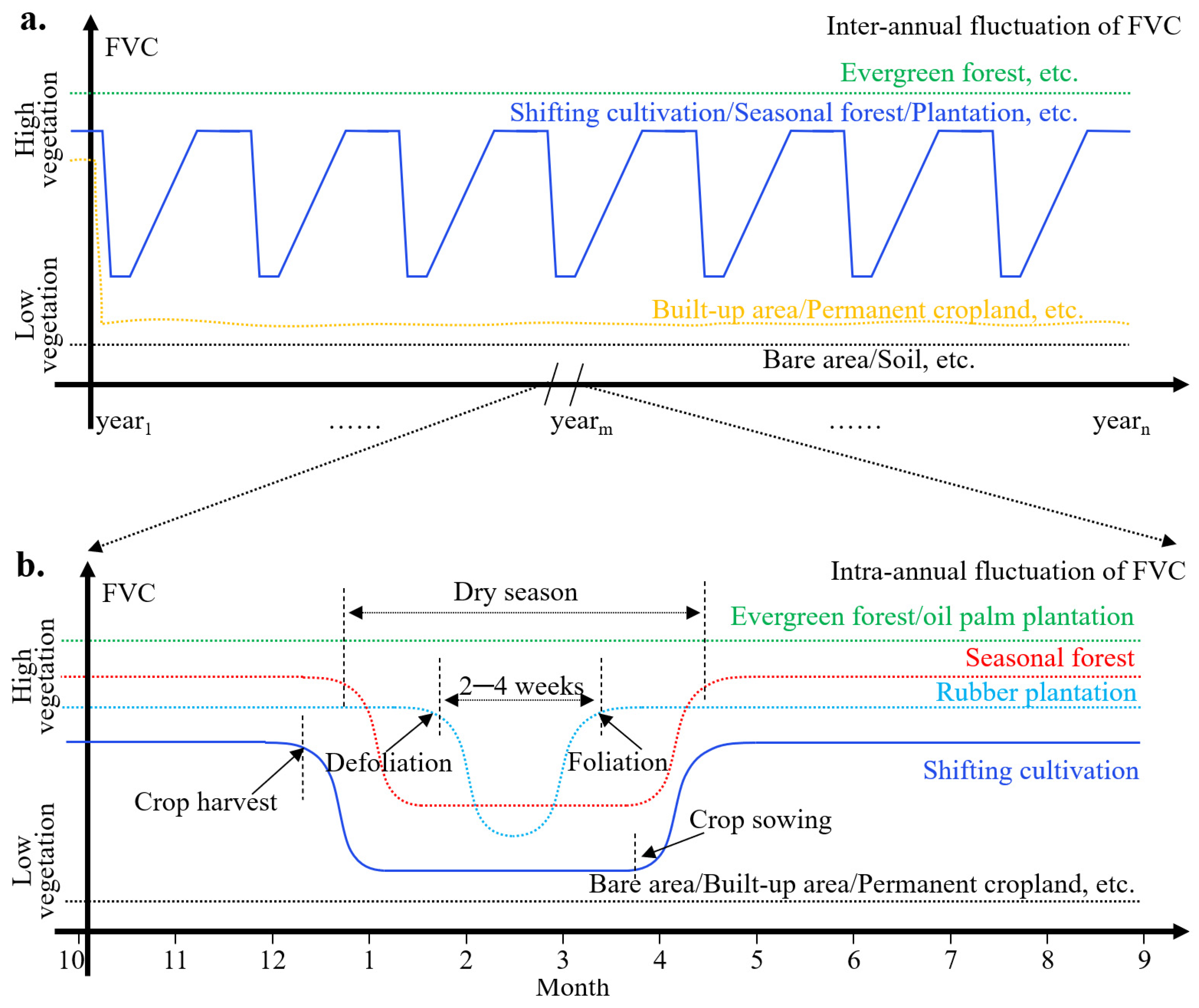
Landsat images are more disturbed by clouds during the rainy season [21]. This study can only use cloudless images in the dry season of the following year as basic data. Within the potential SC area, this study further eliminated non-SC land by analyzing the inter-annual and intra-annual changes in different land types (Figure 5).
Figure 5.
Inter-annual and intra-annual change in different land types. (a) is the inter-annual fluctuation of FVC. (b) is the intra-annual fluctuation of FVC.
According to the working principle of the LC algorithm (Section 2.3), evergreen forests, permanent cropland, built-up, and bare area have been removed from the potential SC area. Pixels that are in the low vegetation state for more than ten consecutive years are also classified as non-SC. Based on the inter-annual fluctuation of FVC, it was found that, in addition to SC, seasonal forest and seasonal plantation [25] also had repetitive disturbance characteristics (Figure 5a). To exclude seasonal forests and seasonal plantations, this study further analyzed their intra-annual changes (Figure 5b). Based on observations over 32 years (1988–2020), SC is in a low vegetation state from October (crop harvest) to May (crop growth). The deciduous period of seasonal forests mainly occurs between January and April. Seasonal plantations (rubber plantations, teak plantations, etc.) have a shorter deciduous period (2–4 weeks) due to human management. This is consistent with existing research [26]. The inter-annual defoliation (leaf shedding) and foliation (emergence of new leaves) signals of seasonal trees thus lay the physiological and phenological basis for delineating seasonal plantations [27].
Based on the information from these years, we identified and removed seasonal forests and seasonal plantations separately (Section 2.4.1). Although an oil palm plantation is an evergreen plantation, it has special radar reflection characteristics [28]. Radar bands from Sentinel-1 image were used to identify and remove oil palm plantations (Section 2.4.2). We used masks from the Joint Research Centre’s Global Surface Water (GSW) dataset to remove water-flooded areas [20]. Finally, we completed the mapping of SC.
2.4.1. Seasonal Plantation Identification
Because of the defoliating and foliating characteristics (Figure 5b), we use a Landsat-based normalization method for identifying seasonal plantations. Landsat-derived FVC between two temporal windows (late January to February and March to early April) was selected to develop multiple normalization methods. Considering the distinguishable characteristics of the FVC, we further extracted the target pixels of two FVC maps during the foliation phase () and defoliation phase (). The RFVC was also established using the normalization principle with two FVC values of seasonal plantations within two temporal windows in which the FVC showed inverse changes.
The value range of the RFVC varies from −1.0 to +1.0. Overall, seasonal plantations can be identified as undergoing defoliation–foliation changes with the corresponding negative RFVC values (i.e., RFVC < 0) within the two temporal windows in the same year. In the same way, two temporal windows (early January and April to early May) corresponding to seasonal forests were used to identify seasonal forests. Although there is some confusion between seasonal forests and seasonal plantations, both are areas that should be removed. For our purpose of identifying SCs, it is not necessary to precisely distinguish seasonal forests from plantations.
2.4.2. Oil Palm Plantation Identification
Oil palm detection requires the preparation of Sentinel-1 data and the application of unsupervised classification in GEE. In addition to VV and VH yearly means, we added the VH/VV difference and the summed average (SAVG) texture metrics from the Gray Level Co-occurrence Matrix around each pixel of every band (radius of three pixels).
We randomly allocated 100,000 training points. The application of unsupervised classification returns the optimal number of clusters (around 15) to fit the sample. Each cluster represents one land cover class (or what the algorithm recognizes as having a similar pattern). Subsequently, we identified those clusters that correspond to oil palm areas by comparing them with very high-resolution imagery. For the specific classification process, we refer to the code of Olga, etc. [29]. We find that this classification result has some confusion in the built-up area. However, as the purpose of this study was only to identify the SC area, the partial confusion of oil palm plantations in built-up areas did not affect our purpose.
2.5. Validation and Correction
2.5.1. Result Validation
To rigorously assess the accuracy of the LandCycler outputs while ensuring adequate representation of rare but ecologically significant high-cycle shifting cultivation areas, a stratified random sampling design was employed. The stratification was based on the spatial distribution of cycle numbers derived from the initial LCm model output. This ensured that the validation dataset included proportional representation across all cycle categories (ranging from 1 to 6 cycles). A total of 1052 validation points were randomly generated within these strata. It is important to note that the LCm output was used exclusively for the purpose of allocating sampling strata to efficiently capture landscape variability. The reference labels (ground truth) for these 1052 points were determined independently of the LandCycler model outputs. Specifically, the land use history (presence of shifting cultivation and number of cycles since 1988) for each point was manually interpreted by experienced remote sensing analysts using the full archive of dry-season Landsat imagery available on the GEE platform, supplemented by high-resolution historical imagery from Google Earth. This visual interpretation served as the independent reference dataset against which the producer’s accuracy, user’s accuracy, and cycle number accuracy of LCm, LCp, and LCn were evaluated (Table 1).
Table 1.
Evaluation results of SC-identification accuracy before adjustment.
The validation results show that the accuracy of SC-identification (user’s accuracy of SC, average accuracy of cycle number, cycle accuracy) by LCm, LCp and LCn models reaches (76.91%, 69.11%, 56.7%), (77.17%, 64.58%, 54.22%) and (72.61%, 58.08%, 24.97%). In SC, pixels with low cycle numbers, the judgment accuracy of LC and the average cycle number accuracy are satisfactory. The three models all show the law that the accuracy gradually decreases with the increase in the number. However, 90% of the SC pixels had 4 or fewer times of deforestations. In contrast, the overall performance of the LCm model and LCp is better than that of LCn. From the perspective of LCm and LCp, the three accuracies in the pixels with the cycle number less than 4 (more than 75% of the total SC pixels) exceed 80%, 85%, and 65%, respectively. When the cycle number is 1, the accuracy of LCm is the highest (81.01%, 99.61%, and 66.28%). Although LCn has lower accuracy, it outperforms LCm and LCp in SC pixels with high cycle numbers. Overall, the accuracy decreases with higher cycle numbers.
2.5.2. Error Evaluation and Correction
The evaluation results show that the detected cycle number is generally larger than the actual results, and the larger the cycle number, the greater the error (Table 2). The error of LCn is much larger than that of LCm and LCp. Therefore, the cycle number of the LC algorithm should be dominated by LCm and LCp and be corrected in a smaller direction. From the accuracy in Section 2.5.1, LCn has higher SC-identification accuracy for high cycle numbers than LCm and LCp. Therefore, it is also necessary to adjust the SC pixels with high cycle numbers according to LCn.
Table 2.
Average error of cycle numbers.
Through visual validation, it is found that the error mainly comes from two locations: the boundary between cropland and forest and rural settlements. Since the tree canopy varies in size from year to year, the FVC values of these mixed pixels are extremely unstable. Therefore, these unstable pixels are easily identified as pseudo-SCs with high cycle numbers and short fallow periods. For a pixel with a high cycle number, when the results of LCn are inconsistent with those of LCm and LCp, the pixel usually does not belong to SC but is an unstable pixel.
Combining the features of the error, this study forms the adjusted SC mapping results by fusing the advantages of the three models. The fusion process of cycle numbers is divided into three steps:
Step 1: By comparing the cycle number of LCm and LCp the minimum value is selected.
Step 2: The area where the cycle number is 1, where the result of LCm is selected.
Step 3: Pixels with a large difference between the three cycle numbers (difference between the maximum and the minimum value) are removed. When the maximum value is 4, pixels with a difference greater than 2 are removed. When the maximum value is greater than 4, pixels with a difference value greater than 1 are removed.
For the corrected cycle number, we recalculated the user’s accuracy, average accuracy, and cycle consistency. In addition, this study selected 895 30 m buffers that belong to SC by experienced professionals. Based on these buffers, we verified the producer’s accuracy of the results. Section 3 is the show and analysis of the detected results.
3. Results
3.1. Accuracy of Results
3.1.1. Cycle Numbers of SC
The evaluation results show that the identification accuracy (user’s accuracy) of SC in this study reached 81.37% (Table 3). The producer’s accuracy based on 1000 known SC pixels is 82.12%. Although the cycle accuracy of the SC is only 63.32%, the average number of deforestations in the region is more meaningful. The average accuracy of this study is as high as 83.71%. Among them, the average accuracy of the SCs with the highest proportion (one, two and three times) reached 96.47%, 89.52% and 80.45%, respectively. More than 98% of SC in Southeast Asia have repeated deforestation four times or less. Therefore, the identification result of cycle numbers of SC is effective.
Table 3.
Evaluation results of SC-identification accuracy.
3.1.2. Fallow Period of SC
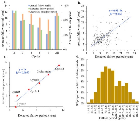
The consistency between the detected fallow period and the actual fallow period was as high as 96% (Figure 6a). As the number of cycles increases, the detected accuracy gradually decreases while the average fallow period decreases. There is an overall linear relationship between the detected fallow period and the actual fallow period (R2 = 0.832, Figure 6b). The lowest accuracy detected in the fallow period was 81.92% when the cycle number is 6. The larger the number of cycles, the shorter the fallow period (Figure 6c). By counting the average fallow period of different cycle numbers, the directly proportional coefficient between the detected fallow period and the actual fallow period is 1 (R2 = 0.997). Both the detected fallow period and the actual fallow period are mainly distributed between 10 ± 3 years (Figure 6d).
Figure 6.
Accuracy of the fallow period. (a) is the average fallow period in different SCs. (b) is accuracy detected in the fallow period. (c) is the accuracy detected in average fallow period. (d) is the SC proportion in different fallow periods.
3.2. Spatial Characteristics of SC in Southeast Asia
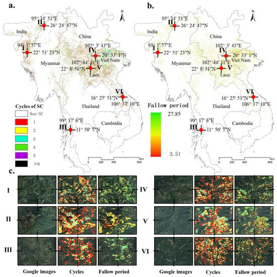
SC is mainly distributed in the mountainous areas of northern Southeast Asia. The total area of SC is as high as 16.79 × 10⁴ km2, which is close to 30% of the permanent cropland in Southeast Asia. These SCs are mainly distributed in two agglomeration areas: the mountainous area at the junction of China–Myanmar–Laos–Vietnam (67.64%), and the mountainous area at the junction of Myanmar–India (16.23%). Between 1988 and 2020, the number of cycles of SC is mainly between 1 and 4 (Figure 7a, Table 3). Likewise, the fallow period for SC is mainly 10 ± 3 years (Figure 7b, Table 3). From a spatial view, the average cycle numbers present: northern Vietnam (3) > northern Laos (2) ≥ India–Myanmar junction (2). The average fallow period is the opposite: northern Vietnam (9 years) ≤ northern Laos (9 years) < India–Myanmar junction (10 years).
Figure 7.
Spatial characteristics of SC in Southeast Asia. (a) is the cycle number; (b) is the fallow period. According to the characteristics of the spatial distribution, this study selected six typical regions for enlarged display ((c)-Figure (I–VI)).
3.3. Characteristics of SC in Different Countries
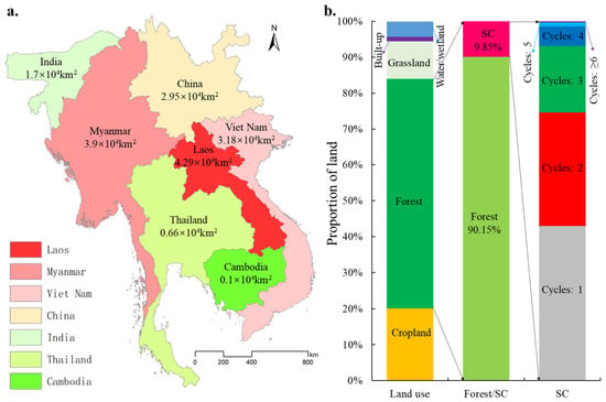
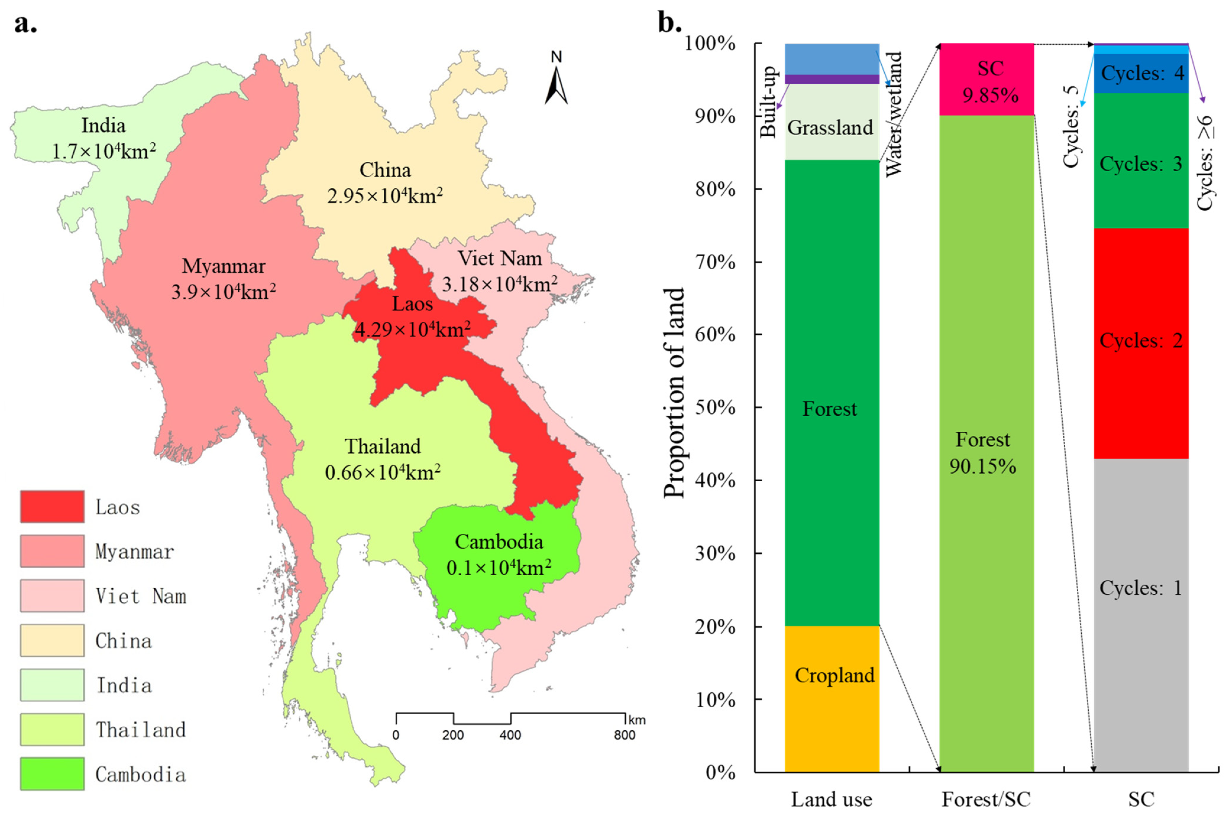
In terms of quantity, Laos, Myanmar and Vietnam have the largest SC scale, reaching 4.29 × 10⁴ km2, 3.9 × 10⁴ km2, and 3.18 × 10⁴ km2 respectively (Figure 8a). In contrast, the SC area of Yunnan Province in China is smaller than neighboring Laos, Myanmar, and Vietnam, at only 2.95 × 10⁴ km2. This is consistent with the significant decrease in SC in Yunnan since the 1980s, largely driven by the expansion of permanent cropland [30]. Their SC area accounts for 67.72% of the total SC area in Southeast Asia. Cambodia has the smallest SC area, less than 0.10 × 10⁴ km2. In terms of the proportion of forests involved in SC (PFISC), SC accounts for nearly 10% of the total forest in Southeast Asia (Figure 8b).
Figure 8.
Area characteristics of SC in different countries. (a) the spatial characteristics of SC area. (b) the proportion characteristics of SC.
Laos, Vietnam, and Assam in India have the largest PFISC, reaching 22.38%, 14.19%, and 11.49% respectively (Figure 9). Similarly, Cambodia has the smallest PFISC at 1.15%. From the perspective of farming mode, Laos is the only country with SC as its main farming mode (a country where the scale of SC is larger than the scale of permanent cropland). The scale of SC in Laos is 239.30% of its permanent cropland, compared to 1.7% in Cambodia and 3.6% in Thailand. With the increase in the cycle number of SC, the SC scale shows an exponentially decreasing trend (Figure 9). The same as the verification result in Section 3.1.1 is that more than 98% of SC in Southeast Asia have repeated deforestation four times or less during 1988–2020 (Table 3).
3.4. Impact Factors of the SC Distribution
In addition to the impact of elevation at the macro-scale, SC in Southeast Asia is mainly distributed in mountainous areas [31], and socioeconomic factors have a much greater impact on the cycle number of SC than natural factors at the micro-scale (Figure 10a,b,f). The distribution of SC with different cycles number is significantly affected by distance from settlements (DS, Figure 10b, r = −0.98, R2 = 0.95) and distance from roads (DR, Figure 10a, r = −0.97, R2 = 0.93).
Figure 9.
Proportion characteristics of SC in different countries.
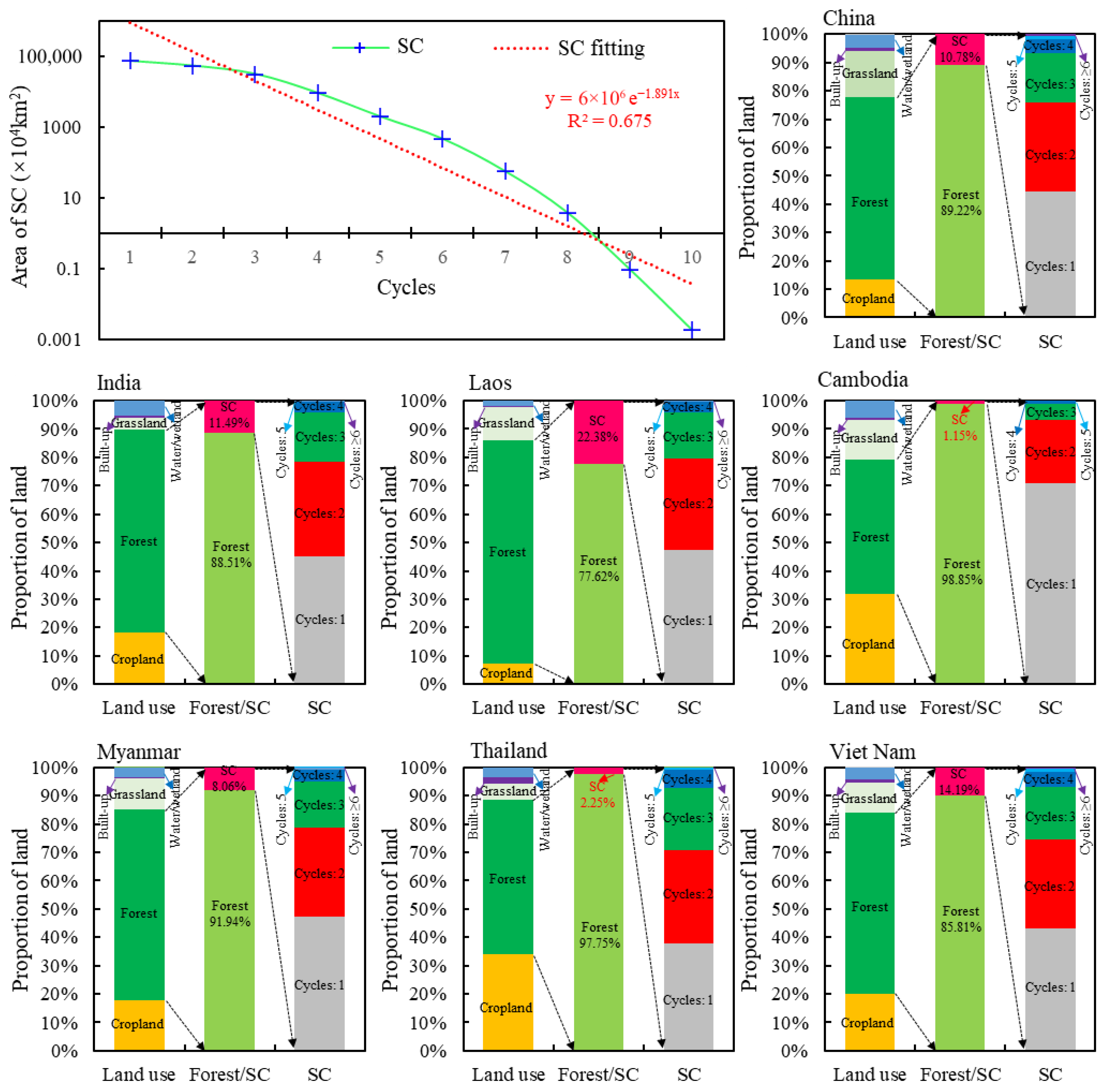
Figure 10.
Impact factors of the SC distribution. The road and residential area datasets are sourced from the 10 m resolution ESA WorldCover 2020 dataset on the GEE platform. (a) the relationship between DR and cycles. (b) relationship between DS and cycles. (c) the synergistic effect of DR and DS on the cycles. (d) the relationship between slope and cycles. (e) relationship between DEM and cycles. (f) the synergistic effect of different factors on the cycles.
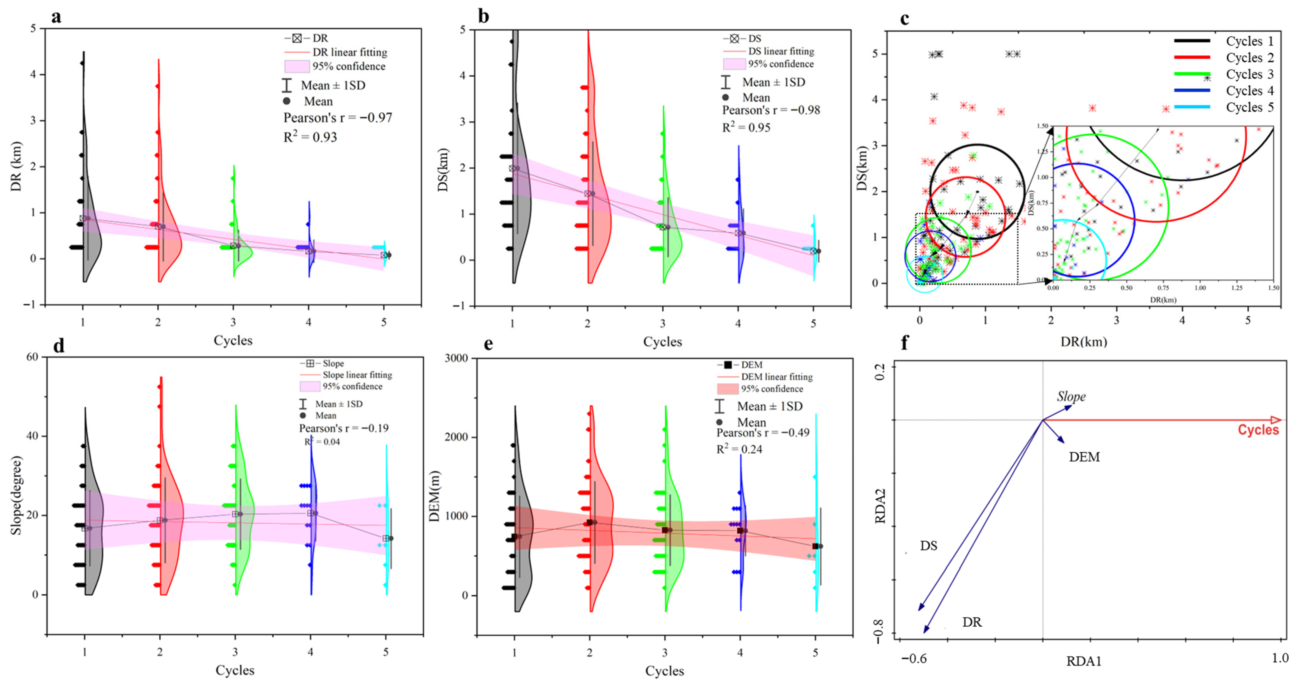
From a socioeconomic perspective, regions with greater ssocioeconomicimpact have a greater cycle number of SC (Figure 10c). According to the two indicators of DS and DR, we draw the sosocioeconomicmpact ellipse corresponding to different cycle numbers. The point corresponding to the mean of DR and DS is the center of the ellipse, and a standard deviation of DR and DS is the horizontal semi-axis and vertical semi-axis, respectively. The reciprocal of the distance from the center of the ellipse to the origin of the coordinates is the socioeconomic impact intensity. The length of the minor semi-axis of the ellipse is uncertain. As the intensity of socioeconomic impact increases, the cycle number gradually increases, and the uncertainty of the cycle number gradually decreases. The socioeconomic impact corresponding to one cycle is the smallest, the center of the ellipse is (0.88, 1.99), and its corresponding uncertainty is the largest at 0.91 km. On the contrary, the socioeconomic impact corresponding to five cycles is the largest, the center of the ellipse is (0.16, 0.59), and its corresponding uncertainty is the smallest at 0.09 km.
In contrast, at the micro-scale, there is no significant correlation between elevation changes (r = −0.19, R2 = 0.04) and slope (r = −0.49, R2 = 0.24) and the cycle number of SC (Figure 10d–f). But all SC is mainly distributed around the slope of 18 ± 5° and the elevation of 800 ± 300 m. Redundancy analysis (RDA) also shows that both DR and DS are significantly negatively correlated with the cycle number of SC, while elevation and slope have no significant effect on the cycle number of SC (Figure 10f).
4. Discussion
4.1. Methodological Application
The current identification methods of SC mainly include sampling statistics based on field surveys [10] and small-scale visual identification based on images [16]. The biggest contribution of this study is to propose the LandCycler algorithm to quickly identify SC in a large area from the perspective of remote sensing. The validation results show that the accuracy of the LandCycler for the identification of SC is satisfactory (producer’s accuracy and user’s accuracy achieved 82.12% and 81.37%, respectively). This has completely exceeded the accuracy (producer’s accuracy of 45.1% and user’s accuracy of 74.4%) of the current attempts to use remote sensing to identify SCs in a small area [16]. Several studies have shown that trajectory-based change detection for the first and last epochs is often unreliable because there are no images before or after the Landsat imagery in the time series [24]. This is also the main reason why our cycle accuracy is only 63.32% (Table 2). In terms of the accuracy of determining the cycle number and the fallow period, the average accuracy is as high as 83.71% and 96%, respectively. Since there are still gaps in the identification of cycles and fallow periods based on remote sensing, we consider this result to be satisfactory.
Based on the LandCycler algorithm, this study is also the first to realize large-scale SC mapping, which provides the possibility for global SC mapping. Compared with a large number of SC plots with small mountain patches, the mapping result of the current one-degree cell resolution is flawed [3]. In addition to the southeast, this form of cultivation remains widespread [32], the majority in the Americas (41%) and Africa (37%). For different regions, the LC algorithm only needs to adjust different FVC thresholds. Furthermore, the algorithm need not be limited to Landsat images. Conceptually, it is easy to envision time series applied to other high-resolution satellite imagery, including Sentinel-2 or Gaofen-1, etc.
4.2. Implications for Sustainable Management
In Montane Mainland Southeast Asia (MMSEA), shifting cultivation has been the dominant land use practice for centuries, and today remains an important subsistence agriculture system [33]. Consistent with the existing statistics, SC in Southeast Asia is mainly distributed in the northern mountainous areas [3]. This is mainly because the mountainous areas are mainly distributed in the northern part of Southeast Asia. The large plains in southern Southeast Asia are more suitable for permanent cropland [34]. Consistent with the existing research [16], DS and DR affect the microscopic distribution of SCs. Consistent with the relevant interview findings [11], our results also show that the practice of SC was more frequently conducted near the villages. Villages and permanent cropland are mainly located in valley with lower elevations and smaller slopes, while areas with higher elevations and larger slopes are not conducive to crop cultivation [35,36], which may be the main reason why SCs are mainly distributed at slopes of 18 ± 5° and elevations of 800 ± 300 m. Most pointed out that the fallow period in Southeast Asia has gradually shortened, averaging 8–10 years [37]. This study shows a fallow period of 10 years in Southeast Asia, which is consistent with the conclusions of the current study [37]. While both elevation and slope exhibit clear constraining effects on the spatial distribution of SC, they do not appear to regulate cultivation intensity within that niche. This decoupling can be understood through a hierarchical framework of land use determinants. Topography acts as a first-order “filter” that delineates where SC is biophysically feasible: areas above ~1100 m are thermally unsuitable for reliable crop maturation, while areas below ~500 m have been largely converted to permanent cropland or settlements. Similarly, slopes exceeding ~23° are too steep for safe cultivation, while flat terrain is preferentially allocated to intensive agriculture. Consequently, SC is compressed into a relatively homogeneous topographic zone.
Increased population pressure and regulations limiting access to land have resulted in more dramatic forest changes and shorter fallow periods [5]. The decline in soil fertility accelerated by shorter fallow periods is expected to be a major constraint in slash-and-burn crop production systems [38,39]. Large-scale and rapid monitoring methods for agriculture and forestry are essential [30]. Our findings can provide tools for forest change detection and SC dynamic detection. Furthermore, our mapping results can provide a basis for sustainable agroforestry management and planning. In addition, our mapping results can provide a basis for planning, which not only affects ecological security and food security, but also is an important support for sustainable agroforestry management. Accurate assessment of the scale and spatial distribution of SCs is an indispensable way to improve the productivity of land resources. Some specialists have pointed to shifting cultivation as one of the drivers of forest degradation and soil deterioration [40]. However, other scholars believe that if an appropriate fallow period is used, the SC not only solves the food problem, but also provides ecological services [4]. Shifting cultivation represents a critical opportunity for low-cost forest restoration whilst diversifying income streams of marginalized communities across a vast area [41]. The first task in resolving this debate is to accurately assess the scale and location of SC, the frequency of shifting, and the fallow period. This work just fills this research gap. Furthermore, this mapping result has important implications for the future success of the Forest Land Allocation policy as well as REDD+ [12,42]. Therefore, the accurate identification of SCs provides a base map for reasonable planning and sustainable development policies [43].
4.3. Limitations and Uncertainties
To improve the operation speed of the LandCycler algorithm, this study adopts a relatively simple identification method: the threshold method based on FVC. Limited by the image resolution and the cloud in the rainy season in tropical regions, it is difficult to further improve the identification of SC cycles and fallow periods. Judging from the evaluation results, the accuracy is already sufficient to support the identification of the SC. With the continuous accumulation of images with a higher spatial and temporal resolution, the accuracy of the algorithm is expected to be further improved.
In addition, the 30 m-resolution images have poor stability at the junction of forest–cropland and the rural settlements. Pixels with spurious changes in value per year are easily misidentified as SCs with a high cycle number and short fallow periods. Due to the cloud removal operation and image overlap, the large difference in the number of valid images in different regions makes the accuracy of LCn very low. However, from the validation results, the identification accuracy of LCn is better than that of LCm and LCp in high cycle numbers. Therefore, the LCn has been used to assist in adjusting the SC area with a high cycle number, thereby eliminating unstable pixels with spurious change in the LCm and LCp results.
5. Conclusions
The main contribution of this study is to build a LandCycler algorithm for rapid and large-scale identification of SC based on Landsat images. In Southeast Asia, the accuracy of this algorithm in identifying SC, detecting the average cycle number, and calculating the average fallow period is 81.37%, 83.71%, and 96%, respectively.
The biggest finding of this study is that the total area of SC is as high as 16.79 × 10⁴ km2, which uses almost 10% of the total forest. These SCs are mainly distributed in the mountainous areas of northern Southeast Asia (83.87%). Meanwhile, this study found that the average cycle number and the average fallow period of SC in Southeast Asia are 2 times and 10 years, respectively during 1988–2020. More than 98% of SC in Southeast Asia have repeated deforestation four times or less. The shorter the distance from DS and the distance from DR, the larger the cycle number of SC. Although there was no significant correlation between elevation and slope and the cycle number of SC, SCs were mainly distributed at slopes of 18 ± 5° and elevations of 800 ± 300 m.
Funding
This research was funded by the National Natural Science Foundation of China (Grant No: 42401082), Future Star Program of Chinese Academy of Sciences (Grant No: 2026000103), and Project funded by China Postdoctoral Science Foundation (Grant No: 2024M763351).
Data Availability Statement
The data supporting the findings of this study were obtained from multiple public sources. Landsat and Sentinel data are sourced from public data archives and GEE’s user team (https://code.earthengine.google.com/). European Space Agency (ESA) WorldCover 2020 data are sourced from the Land cover (Global—10m—2020)—ESA WorldCover (https://data.apps.fao.org/catalog/dataset/378e9df5-3814-4a80-bb47-e25df0543634) (accessed on 18 December 2025). The population density data set used in this study is obtained from the Center for International Earth Science Information Network (https://www.data4sdgs.org/initiatives/popgrid-data-collaborative) (accessed on 18 December 2025), and can be directly obtained by calling id “CIESIN/GPWv411/GPW_Population_Density” in GEE. DEM data comes from the Global Digital Elevation Model (https://data.casearth.cn/thematic/dem?lang=zh) (accessed on 8 October 2025).
Acknowledgments
I confirm that all individuals mentioned in the acknowledgements section have consented to their inclusion. I would like to thank my colleagues from China University of Geosciences (Beijing) and the University of Copenhagen for their technical assistance and work environment support. We also want to thank the anonymous reviewers for their valuable suggestions and comments that contributed to improving the quality of the manuscript.
Conflicts of Interest
The author declares no conflicts of interest.
Abbreviations
The following abbreviations are used in this manuscript:
| SC | Shifting cultivation |
| MMSEA | Montane Mainland Southeast Asia |
| GEE | Google Earth Engine |
| LC | LandCycler |
| LCm | LC in median model |
| LCp | LC in probabilistic model |
| LCn | LC in number model |
| FVC | Fractional Vegetation Cover |
| NC | Number of cycles |
| TFL | Total fallow period length |
| FP | Fallow period |
| GSW | Global Surface Water |
References
- Mertz, O.; Bruun, T.B.; Jepsen, M.R.; Ryan, C.M.; Zaehringer, J.G.; Hinrup, J.S.; Heinimann, A. Ecosystem Service Provision by Secondary Forests in Shifting Cultivation Areas Remains Poorly Understood. Hum. Ecol. 2021, 49, 271–283. [Google Scholar] [CrossRef] [Scilit]
- Liu, S.D.; Zhang, J.; Wang, L.; Ciais, P.; Zhang, J.J.; Penuelas, J.; Nath, B.; Jacquet, I.; Wu, X.; Ding, S.P.; et al. Mapping previously undetected trees reveals overlooked changes in pan-tropical tree cover. Nat. Commun. 2025, 16, 5561. [Google Scholar] [CrossRef] [Scilit]
- Heinimann, A.; Mertz, O.; Frolking, S.; Christensen, A.E.; Hurni, K.; Sedano, F.; Chini, L.P.; Sahajpal, R.; Hansen, M.; Hurtt, G. A global view of shifting cultivation: Recent, current, and future extent. PLoS ONE 2017, 12, e0184479. [Google Scholar] [CrossRef] [Scilit]
- Fox, J.; Castella, J.C.; Ziegler, A.D. Swidden, rubber and carbon: Can REDD plus work for people and the environment in Montane Mainland Southeast Asia? Glob. Environ. Change-Hum. Policy Dimens. 2014, 29, 318–326. [Google Scholar] [CrossRef] [Scilit]
- Roder, W.; Phengchanh, S.; Maniphone, S. Dynamics of soil and vegetation during crop and fallow period in slash-and-burn fields of northern Laos. Geoderma 1997, 76, 131–144. [Google Scholar] [CrossRef] [Scilit]
- Grogan, K.; Pflugmacher, D.; Hostert, P.; Kennedy, R.; Fensholt, R. Cross-border forest disturbance and the role of natural rubber in mainland Southeast Asia using annual Landsat time series. Remote Sens. Environ. 2015, 169, 438–453. [Google Scholar] [CrossRef] [Scilit]
- Van Vliet, N.; Mertz, O.; Heinimann, A.; Langanke, T.; Pascual, U.; Schmook, B.; Adams, C.; Schmidt-Vogt, D.; Messerli, P.; Leisz, S.; et al. Trends, drivers and impacts of changes in swidden cultivation in tropical forest-agriculture frontiers: A global assessment. Glob. Environ. Change-Hum. Policy Dimens. 2012, 22, 418–429. [Google Scholar] [CrossRef] [Scilit]
- Zhang, J.; Liu, S.D. Revealing the Process and Mechanism of Non-Main Grain Cropland Expansion in China. Land Degrad. Dev. 2025, 1–13. [Google Scholar] [CrossRef] [Scilit]
- Wang, L.; Liu, S.; Song, W.; Ding, S.; Zhang, J. Global high-resolution forest disturbance type dataset. Earth Syst. Sci. Data 2026, 18, 1601–1617. [Google Scholar] [CrossRef] [Scilit]
- Morales-Barquero, L.; Borrego, A.; Skutsch, M.; Kleinn, C.; Healey, J.R. Identification and quantification of drivers of forest degradation in tropical dry forests: A case study in Western Mexico. Land Use Policy 2015, 49, 296–309. [Google Scholar] [CrossRef] [Scilit]
- Chan, N.; Takeda, S.; Suzuki, R.; Yamamoto, S. Establishment of allometric models and estimation of biomass recovery of swidden cultivation fallows in mixed deciduous forests of the Bago Mountains, Myanmar. For. Ecol. Manag. 2013, 304, 427–436. [Google Scholar] [CrossRef] [Scilit]
- Phelps, J.; Webb, E.L.; Adams, W.M. Biodiversity co-benefits of policies to reduce forest-carbon emissions. Nat. Clim. Change 2012, 2, 497–503. [Google Scholar] [CrossRef] [Scilit]
- Dwyer, J.L.; Roy, D.P.; Sauer, B.; Jenkerson, C.B.; Zhang, H.K.K.; Lymburner, L. Analysis Ready Data: Enabling Analysis of the Landsat Archive. Remote Sens. 2018, 10, 1363. [Google Scholar] [CrossRef] [Scilit]
- Kennedy, R.E.; Yang, Z.G.; Cohen, W.B. Detecting trends in forest disturbance and recovery using yearly Landsat time series: 1. LandTrendr—Temporal segmentation algorithms. Remote Sens. Environ. 2010, 114, 2897–2910. [Google Scholar] [CrossRef] [Scilit]
- Zhu, Z.; Woodcock, C.E. Continuous change detection and classification of land cover using all available Landsat data. Remote Sens. Environ. 2014, 144, 152–171. [Google Scholar] [CrossRef] [Scilit]
- Shimizu, K.; Ota, T.; Mizoue, N.; Yoshida, S. Patch-Based Assessments of Shifting Cultivation Detected by Landsat Time Series Images in Myanmar. Sustainability 2018, 10, 3350. [Google Scholar] [CrossRef] [Scilit]
- Miettinen, J.; Shi, C.H.; Liew, S.C. Deforestation rates in insular Southeast Asia between 2000 and 2010. Glob. Change Biol. 2011, 17, 2261–2270. [Google Scholar] [CrossRef] [Scilit]
- Goldberg, L.; Lagomasino, D.; Thomas, N.; Fatoyinbo, T. Global declines in human-driven mangrove loss. Glob. Change Biol. 2020, 26, 5844–5855. [Google Scholar] [CrossRef] [Scilit]
- Zanaga, D.; Van De Kerchove, R.; De Keersmaecker, W.; Souverijns, N.; Brockmann, C.; Quast, R.; Wevers, J.; Grosu, A.; Paccini, A.; Vergnaud, S. WorldCover 10 m 2020 v100; European Space Agency: Paris, France, 2021. [Google Scholar]
- Pekel, J.F.; Cottam, A.; Gorelick, N.; Belward, A.S. High-resolution mapping of global surface water and its long-term changes. Nature 2016, 540, 418–422. [Google Scholar] [CrossRef] [Scilit] [PubMed]
- Irannezhad, M.; Liu, J.G.; Chen, D.L. Influential Climate Teleconnections for Spatiotemporal Precipitation Variability in the Lancang-Mekong River Basin From 1952 to 2015. J. Geophys. Res.-Atmos. 2020, 125, e2020JD033331. [Google Scholar] [CrossRef] [Scilit]
- Roy, D.P.; Kovalskyy, V.; Zhang, H.K.; Vermote, E.F.; Yan, L.; Kumar, S.S.; Egorov, A. Characterization of Landsat-7 to Landsat-8 reflective wavelength and normalized difference vegetation index continuity. Remote Sens. Environ. 2016, 185, 57–70. [Google Scholar] [CrossRef] [Scilit]
- Song, W.J.; Mu, X.H.; McVicar, T.R.; Knyazikhin, Y.; Liu, X.L.; Wang, L.; Niu, Z.; Yan, G.J. Global quasi-daily fractional vegetation cover estimated from the DSCOVR EPIC directional hotspot dataset. Remote Sens. Environ. 2022, 269, 112835. [Google Scholar] [CrossRef] [Scilit]
- Cohen, W.B.; Healey, S.P.; Yang, Z.; Stehman, S.V.; Brewer, C.K.; Brooks, E.B.; Gorelick, N.; Huang, C.; Hughes, M.J.; Kennedy, R.E. How similar are forest disturbance maps derived from different Landsat time series algorithms? Forests 2017, 8, 98. [Google Scholar] [CrossRef] [Scilit]
- Ziegler, A.D.; Fox, J.M.; Xu, J.C. The Rubber Juggernaut. Science 2009, 324, 1024–1025. [Google Scholar] [CrossRef] [Scilit] [PubMed]
- Guardiola-Claramonte, M.; Troch, P.A.; Ziegler, A.D.; Giambelluca, T.W.; Durcik, M.; Vogler, J.B.; Nullet, M.A. Hydrologic effects of the expansion of rubber (Hevea brasiliensis) in a tropical catchment. Ecohydrology 2010, 3, 306–314. [Google Scholar] [CrossRef] [Scilit]
- Lan, G.Y.; Li, Y.W.; Lesueur, D.; Wu, Z.X.; Xie, G.S. Seasonal changes impact soil bacterial communities in a rubber plantation on Hainan Island, China. Sci. Tot. Environ. 2018, 626, 826–834. [Google Scholar] [CrossRef] [Scilit]
- Descals, A.; Wich, S.; Meijaard, E.; Gaveau, D.L.A.; Peedell, S.; Szantoi, Z. High-resolution global map of smallholder and industrial closed-canopy oil palm plantations. Earth Syst. Sci. Data 2021, 13, 1211–1231. [Google Scholar] [CrossRef] [Scilit]
- Danylo, O.; Pirker, J.; Lemoine, G.; Ceccherini, G.; See, L.; McCallum, I.; Hadi; Kraxner, F.; Achard, F.; Fritz, S. A map of the extent and year of detection of oil palm plantations in Indonesia, Malaysia and Thailand. Sci. Data 2021, 8, 96. [Google Scholar] [CrossRef] [Scilit]
- Liu, S.; Wang, L.; Zhang, J. The dataset of main grain land changes in China over 1985–2020. Sci. Data 2024, 11, 1430. [Google Scholar] [CrossRef] [Scilit]
- Don, A.; Schumacher, J.; Freibauer, A. Impact of tropical land-use change on soil organic carbon stocks—A meta-analysis. Glob. Change Biol. 2011, 17, 1658–1670. [Google Scholar] [CrossRef] [Scilit]
- Burchfield, E.K. Shifting cultivation geographies in the Central and Eastern US. Environ. Res. Lett. 2022, 17, 054049. [Google Scholar] [CrossRef] [Scilit]
- Hurni, K.; Hett, C.; Heinimann, A.; Messerli, P.; Wiesmann, U. Dynamics of Shifting Cultivation Landscapes in Northern Lao PDR Between 2000 and 2009 Based on an Analysis of MODIS Time Series and Landsat Images. Hum. Ecol. 2013, 41, 21–36. [Google Scholar] [CrossRef] [Scilit]
- Ueno, K.; Miyahigashi, A.; Kamata, Y.; Kato, M.; Charoentitirat, T.; Limruk, S. Geotectonic implications of Permian and Triassic carbonate successions in the Central Plain of Thailand. J. Asian Earth Sci. 2012, 61, 33–50. [Google Scholar] [CrossRef] [Scilit]
- He, Y.; Wang, L.; Pei, J.; Liu, S.; Yang, H.; Cao, J.; Li, W.; Niu, Z.; Huang, N.; Xu, X.; et al. Differential vegetation drought adaptability in global karst areas. npj Clim. Atmos. Sci. 2025, 8, 343. [Google Scholar] [CrossRef] [Scilit]
- Prokop, P.; Kruczkowska, B.; Syiemlieh, H.J.; Bucala-Hrabia, A. Impact of topography and sedentary swidden cultivation on soils in the hilly uplands of North-East India. Land Degrad. Dev. 2018, 29, 2760–2770. [Google Scholar] [CrossRef] [Scilit]
- Kameda, C.; Nawata, E. Relationship between fallow period, forest vegetation and weeds in swidden agriculture in northern Laos. Agrofor. Syst. 2017, 91, 553–564. [Google Scholar] [CrossRef] [Scilit]
- Liu, S.; Wang, L.; Zhang, J.; Ding, S. Opposite effect on soil organic carbon between grain and non-grain crops: Evidence from Main Grain Land, China. Agric. Ecosyst. Environ. 2025, 379, 109364. [Google Scholar] [CrossRef] [Scilit]
- Roder, W.; Phengchanh, S.; Keoboulapha, B. Relationships between soil, fallow period, weeds and rice yield in slash-and-burn systems of Laos. Plant Soil 1995, 176, 27–36. [Google Scholar] [CrossRef] [Scilit]
- Hepp, C.M.; de Neergaard, A.; Bruun, T.B. Short-term fallow in extensive upland shifting cultivation systems of Northern Lao PDR: Its role in soil fertility restoration. Land Degrad. Dev. 2018, 29, 2911–2919. [Google Scholar] [CrossRef] [Scilit]
- Morton, O.; Borah, J.R.; Edwards, D.P. Economically viable forest restoration in shifting cultivation landscapes. Environ. Res. Lett. 2020, 15, 064017. [Google Scholar] [CrossRef] [Scilit]
- Borrelli, P.; Robinson, D.A.; Fleischer, L.R.; Lugato, E.; Ballabio, C.; Alewell, C.; Meusburger, K.; Modugno, S.; Schutt, B.; Ferro, V.; et al. An assessment of the global impact of 21st century land use change on soil erosion. Nat. Commun. 2017, 8, 2013. [Google Scholar] [CrossRef] [Scilit] [PubMed]
- Bose, P. Oil palm plantations vs. shifting cultivation for indigenous peoples: Analyzing Mizoram’s New Land Use Policy. Land Use Policy 2019, 81, 115–123. [Google Scholar] [CrossRef] [Scilit]

Disclaimer/Publisher’s Note: The statements, opinions and data contained in all publications are solely those of the individual author(s) and contributor(s) and not of MDPI and/or the editor(s). MDPI and/or the editor(s) disclaim responsibility for any injury to people or property resulting from any ideas, methods, instructions or products referred to in the content. |
© 2026 by the author. Licensee MDPI, Basel, Switzerland. This article is an open access article distributed under the terms and conditions of the Creative Commons Attribution (CC BY) license.