A Feature-Optimized Deep Learning Framework for Mapping and Spatial Characterization of Tea Plantations in Complex Mountain Landscapes

Highlights

What are the main findings?

• A sequential JM–Pearson feature optimization strategy reduced the Sentinel-1/2 candidate feature space from 132 to 28 variables (78.8% reduction) while preserving class separability and suppressing redundancy in complex mountain landscapes.
• The optimized VGG16–UNet++ framework achieved the best tea plantation mapping performance, reaching PA 90.73%, UA 91.14%, OA 97.82%, F1-score 0.9093, and mIoU 0.7968.

What are the implications of the main findings?

• The wall-to-wall tea plantation map can be translated into reproducible ecological indicators, including multi-threshold steep-slope exposure and 1-km tea–forest interface density, for spatial risk assessment.
• The proposed framework provides actionable support for slope-based zoning, ecological restoration, and sustainable management in fragile mountain agroforestry systems.

Abstract

The unchecked expansion of tea plantations onto steep, forest-adjacent slopes in subtropical mountains engenders a conflict between agricultural productivity and ecosystem integrity, particularly by exacerbating habitat fragmentation and soil erosion. While precise monitoring is essential to navigate this trade-off for sustainable management, accurate inventorying remains a challenge due to the plantations’ strong phenological variability, heterogeneous canopy structures, and high spectral confusion with surrounding vegetation. This study proposes a feature-optimized deep learning framework for mapping and characterizing tea plantations in complex landscapes, using Xinyang City, China, as a study area. The framework integrates multi-temporal Sentinel-1/2 observations with a sequential Jeffries-Matusita (JM)-Pearson feature filtering strategy. This approach effectively condenses a 132-variable high-dimensional pool (including optical spectra, vegetation indices, textures, and SAR polarimetry) into a compact 28-feature subset (a 78.8% reduction), preserving critical phenological and structural cues while minimizing redundancy. These optimized predictors drive a hybrid VGG16–UNet++ segmentation network, which couples transfer-learning-based semantic encoding with detail-preserving dense skip fusion. Extensive experiments across 18 model–feature configurations demonstrate that the optimal setting achieves an Overall Accuracy of 97.82%, an F1-score of 0.9093, and a mean IoU of 0.7968. Notably, the method significantly reduces misclassification in rugged, cloud-prone terrain, yielding a User’s Accuracy of 91.14% for tea. Based on the generated wall-to-wall map, we derived two decision-support indicators: multi-threshold steep-slope exposure and a normalized tea–forest interface density. This framework provides actionable, high-precision spatial products to support slope-based zoning, ecological restoration, and sustainable management in fragile mountain agroforestry systems.

1. Introduction

Tea plantations constitute a vital agro-ecosystem in subtropical Asia, serving as a key economic pillar for many producing regions while playing a complex role in ecological balance and rural livelihoods [1,2]. In China, marked demand and government incentives have fueled a dramatic expansion of tea cultivation over the past decade, and this expansion is increasingly encroaching upon ecologically fragile mountainous areas [3]. While the tea industry supports economic development, the conversion of natural forests into monocultures on steep slopes has ignited serious concerns regarding habitat fragmentation, soil erosion, climate regulation, and biodiversity loss [4,5,6]. Consequently, sustainable management requires more than a simple inventory of total plantation area; it demands a comprehensive spatial characterization to reveal where tea is planted (e.g., on steep gradients) and how it interacts with surrounding ecosystems (e.g., tea-forest interfaces). Such spatially explicit intelligence is critical for balancing agricultural production with ecological restoration.

However, accurate mapping and characterization of tea plantations in mountainous terrains present distinctive challenges relative to flatland crops [7,8,9,10]. First, spectral confusion is acute. In complex terrains, tea plantations often exhibit spectral and textural signatures that are highly similar to evergreen forests and shrublands, which makes separation difficult. Second, phonological complexity complicates monitoring. Tea undergoes dynamic seasonal changes, such as leaf flushing, pruning, and harvesting, and these events create temporal variability that single-date imagery cannot capture. Third, landscape fragmentation poses a barrier. Unlike large-scale mechanized farming, mountain tea patches are frequently small, irregular, and separated by topography. This fragmentation demands high-resolution delineation capabilities to preserve boundary details.

Satellite remote sensing, distinguished by its extensive spatial coverage, high spatial resolution, frequent revisit cycles, and rich spectral information, has emerged as an indispensable tool for Land Use and Land Cover (LULC) monitoring across scales ranging from the local to the global [11,12,13,14]. Optical imagery remains the predominant data source for vegetation classification due to its sensitivity to spectral characteristics, yet its operational utility is frequently constrained by atmospheric perturbations, particularly persistent cloud cover and rainfall [15,16]. This limitation is particularly pronounced in tea plantation mapping, as tea gardens are predominantly distributed in complex mountainous terrains where cloud occlusion is frequent and severe. To address this, Synthetic Aperture Radar (SAR) offers all-weather imaging capabilities, providing stable acquisition of structural and dielectric information regardless of meteorological conditions [17]. Consequently, the synergistic integration of optical and SAR data, supplemented by other multi-source variables, has been proven to enhance mapping robustness by compensating for the inherent deficiencies of single-sensor systems [18,19,20]. In this context, Sentinel-1 and Sentinel-2 have been widely adopted as primary data sources for fusion-based land cover monitoring, owing to their superior spatial resolution and complementary imaging mechanisms [21,22]. However, the proliferation of such multi-source and multi-temporal predictors inevitably precipitates the curse of dimensionality. The concomitant redundancy and computational complexity pose major bottlenecks to classifier performance, rendering efficient feature selection essential [23]. Among various strategies, filter-based methods are favored for their computational efficiency, with class-separability metrics like the Jeffreys-Matusita (JM) distance serving as a standard for evaluating discriminatory power [24,25]. Although recent studies have successfully employed JM-based selection for crop mapping, a critical limitation remains: traditional JM approaches typically focus on individual feature separability while neglecting high inter-feature correlation [26,27]. This oversight often leads to the retention of redundant variables (multicollinearity), which can undermine subsequent classification performance [28]. A framework that identifies a compact, low-redundancy, yet highly discriminative feature subset is therefore essential for efficient mapping.

While traditional machine learning classifiers established the foundation for crop mapping, the field has undergone a paradigm shift with the advent of deep learning, particularly in semantic segmentation [29]. Unlike pixel-based approaches, Convolutional Neural Networks (CNNs) facilitate the end-to-end learning of hierarchical features, effectively capturing both the local textures and global contextual semantics required to delineate complex land covers [11,30]. Powerful architectures, such as the UNet family, have demonstrated remarkable success in fine-scale extraction tasks [31]. However, applying these models to fragmented mountain landscapes remains non-trivial. Standard architectures often struggle to balance the trade-off between high-level semantic abstraction and low-level spatial detail–a capability critical for preserving the irregular boundaries of smallholder tea patches [32]. Furthermore, single-stream networks may lack the feature extraction depth required to fully exploit the subtle patterns in fused SAR-optical data [33]. Hybrid models that combine robust feature extractors (e.g., VGG backbones) with dense skip-connection architectures (e.g., UNet++) offer a potential solution to enhance feature transferability and boundary precision. Nevertheless, such optimized configurations remain underexplored in the context of specific agroforestry applications within rugged terrain.

To address the dual needs of accurate inventory and ecological risk assessment, this study proposes a feature-optimized deep learning framework designed for mapping and spatial characterization of tea plantations in complex mountain landscapes. Our contribution is threefold. First, we construct a phenology-aware Sentinel-1/2 fusion dataset and introduce a Pearson-enhanced JM feature filtering mechanism. This novel selection strategy explicitly addresses the multicollinearity issue inherent in traditional separability metrics, ensuring a compact yet highly discriminative feature subset. Second, we engineer a hybrid VGG16-UNet++ architecture, leveraging the deep feature extraction capability of VGG 16 to enhance the nested skip pathways of UNet++, thereby improving the segmentation of fragmented tea patches against a mosaic background. Finally, moving beyond mere classification, we operationalize the mapping results into management-relevant spatial indicators. By quantifying multi-threshold steep-slope exposure (≥10°/12°/15°/20°/25°) and the density of tea-forest interfaces, we provide actionable intelligence for balancing agro-economic expansion with ecological preservation in fragile mountain environments.

2. Study Area and Data Source

2.1. Study Area

The study was conducted in Xinyang City, Henan Province, China (113°53′–114°37′E, 31°42′–32°32′N; covering 18,916 km²), a premier tea-producing region renowned for Xinyang Maojian tea. The region lies in a transitional zone between subtropical and warm temperate climates, characterized by a distinct topographic gradient ranging from mountainous–hilly terrain in the south to alluvial plains in the north. Elevations vary from approximately 100 m to over 1000 m, with a mean annual precipitation of about 1300 mm. These climatic conditions, combined with well-drained acidic soils, create an optimal environment for tea cultivation. Tea plantations are predominantly distributed across low- to mid-elevation hillslopes, ridges, and forest margins, forming a highly fragmented mosaic interspersed with forests, croplands, and built-up areas. In certain subregions, the intensification of tea cultivation has driven the conversion of forests and mixed vegetation on sloping lands. This expansion has increased habitat fragmentation and slope disturbance, exacerbating susceptibility to soil erosion and hydrological alteration. Crucially, these complex biophysical conditions introduce significant challenges for remote sensing, including terrain-induced geometric distortions, topographic shadowing, and severe spectral mixing. These factors necessitate a robust mapping framework capable of accurately delineating tea plantations within this fragile mountain agroforestry system.

According to local phenological characteristics, tea harvesting is categorized into three primary seasons: spring tea (late March to mid-May), summer tea (June to July), and autumn tea (August to September). During winter (December to February), tea plants enter a dormancy phase characterized by minimal physiological activity. The seasonal harvesting schedule is summarized in

Table 1. Harvesting schedule and phonological stages of Xinyang Maojian tea.

Picking Period		Date	Picking Stage
Spring Tea	Tea picked before Qingming Festival	From the end of March to the Qingming Festival	First Picking
	Tea leaves picked between the Qingming Festival and the Grain Rain period	From after the Qingming Festival to the late April
	Tea leaves picked between the Grain Rain period and the beginning of summer	From the late April to the middle of May
Summer Tea	From June to July	Second Picking	From June to July
Autumn Tea	From August to September	Third Picking	From August to September
Wintering Period	From December to February of the following year	Wintering Period	From December to February of the following year

.

2.2. Sentinel-1/2 Image Data

Multi-temporal Sentinel-1 (C-band SAR) and Sentinel-2 (MSI) datasets were synergistically utilized to support tea plantation mapping. To better describe the satellite observation strategy, the acquisition of these datasets was designed according to the phenological characteristics of Xinyang Maojian tea, so that key seasonal stages of tea growth could be effectively represented in the remote sensing observations. Sentinel-1, operating mainly in Interferometric Wide Swath (IW) mode, provides a spatial resolution of approximately 5 m × 20 m with a 250 km swath width and a 6-day revisit cycle [34] (Zhang et al., 2025). Standard pre-processing workflows, including precise orbit correction, radiometric calibration, and Refined Lee speckle filtering, were applied to ensure radiometric consistency across different growth stages. Sentinel-2 offers a 5-day revisit cycle with 13 spectral bands (10 m for visible/NIR, 20 m for red-edge/SWIR, and 60 m for atmospheric bands) over a 290 km swath [25,35]. Scenes free from clouds and stripe noise were prioritized and processed from Level-1C to Level-2A reflectance using standard geometric and radiometric corrections. In addition, Sentinel-1 observations provided dual-polarization backscatter information (VV and VH), whereas Sentinel-2 observations provided multi-spectral reflectance information, allowing complementary characterization of vegetation spectral properties and surface structural conditions.

Image acquisition dates were selected to align with the distinct phenological stages of Xinyang Maojian tea. Specifically, imagery from four key periods was utilized: May 2022, June 2022, August 2022, and February 2023, as detailed in

Table 2. Details of Sentinel imagery acquisition and atmospheric conditions.

Phenological Period	Sentinel-1/2 Image Acquisition Date	Image Quality
Spring Tea	May 2022	Weather is good, clear sky
Summer Tea	June 2022	Weather is good, with few clouds
Autumn Tea	August 2022	Weather is good, clear sky
Wintering Period	February 2023	Weather is good, with few clouds

. These four periods respectively correspond to the spring tea stage, summer tea stage, autumn tea stage, and winter dormancy stage, thereby enabling the capture of complementary temporal differences in canopy vigor, vegetation structure, and seasonal spectral response. Such a phenology-oriented observation design improves the separability of tea plantations from surrounding forests, cultivated land, and other vegetation types. All datasets were accessed and processed via the Google Earth Engine (GEE) platform. Sentinel-2 imagery served as the spatial reference for geo-referencing. The pre-processed SAR and optical data were co-registered to generate a fused dataset, integrating complementary spectral and structural features. Based on these co-registered multi-temporal satellite observations, spectral bands, vegetation indices, texture features, and SAR polarization features were subsequently derived to construct the candidate feature space for the following feature optimization and deep learning classification.

2.3. Sample Data

To construct and validate the classification model, a comprehensive ground reference dataset was developed through an extensive field survey conducted in Xinyang City in December 2022. During the field campaign, representative tea plantation areas and other land-cover types were systematically investigated, and homogeneous land-cover patches were identified as candidate sampling units. Field observations were cross-referenced with high-resolution Google Earth imagery to ensure label accuracy. Specifically, sample locations were determined by combining in-situ observations and visual interpretation of high-resolution imagery. Only homogeneous regions with clear land-cover boundaries were selected, while mixed pixels, transitional zones, and areas affected by shadow or seasonal disturbance were excluded to improve label reliability. The sample dataset encompasses five major land cover categories: tea plantations, water bodies, forests, built-up areas, and cultivated land. A stratified random sampling strategy was adopted to ensure statistical representativeness and mitigate selection bias. The stratification considered not only differences among land-cover categories, but also the intra-class heterogeneity of tea plantations. In particular, tea samples were selected to cover variations in vegetation density, topographic position, and planting structure, so that the reference dataset could better represent the spatial complexity of tea plantations in mountainous environments. This approach accounted for the intra-class variability of tea plantations, covering diverse vegetation densities, topographic positions, and planting types. The final dataset was partitioned into a training set (70%) and a validation set (30%), maintaining balanced class proportions in both subsets to prevent model overfitting and ensure objective performance evaluation. Furthermore, the geographic distribution of samples was rigorously controlled to ensure uniform spatial coverage across the study area, thereby minimizing spatial autocorrelation and enhancing the model’s generalization capability in complex terrain. To further reduce spatial dependence, excessive concentration of samples within the same contiguous patch was avoided, and samples were distributed across different parts of the study area as far as possible. This strategy improved both the representativeness and the robustness of the training and validation datasets. Detailed sample distribution statistics are provided in

Table 3. Summary of ground reference samples used for model training and validation.

Category	Number of Training Set Samples	Number of Validation Set Samples	Total Number
Tea	3827	1640	5467
Water	3672	1573	5245
Forest	3868	1658	5526
Building	3602	1543	5145
Cultivated land	3862	1655	5517

.

3. Methodology

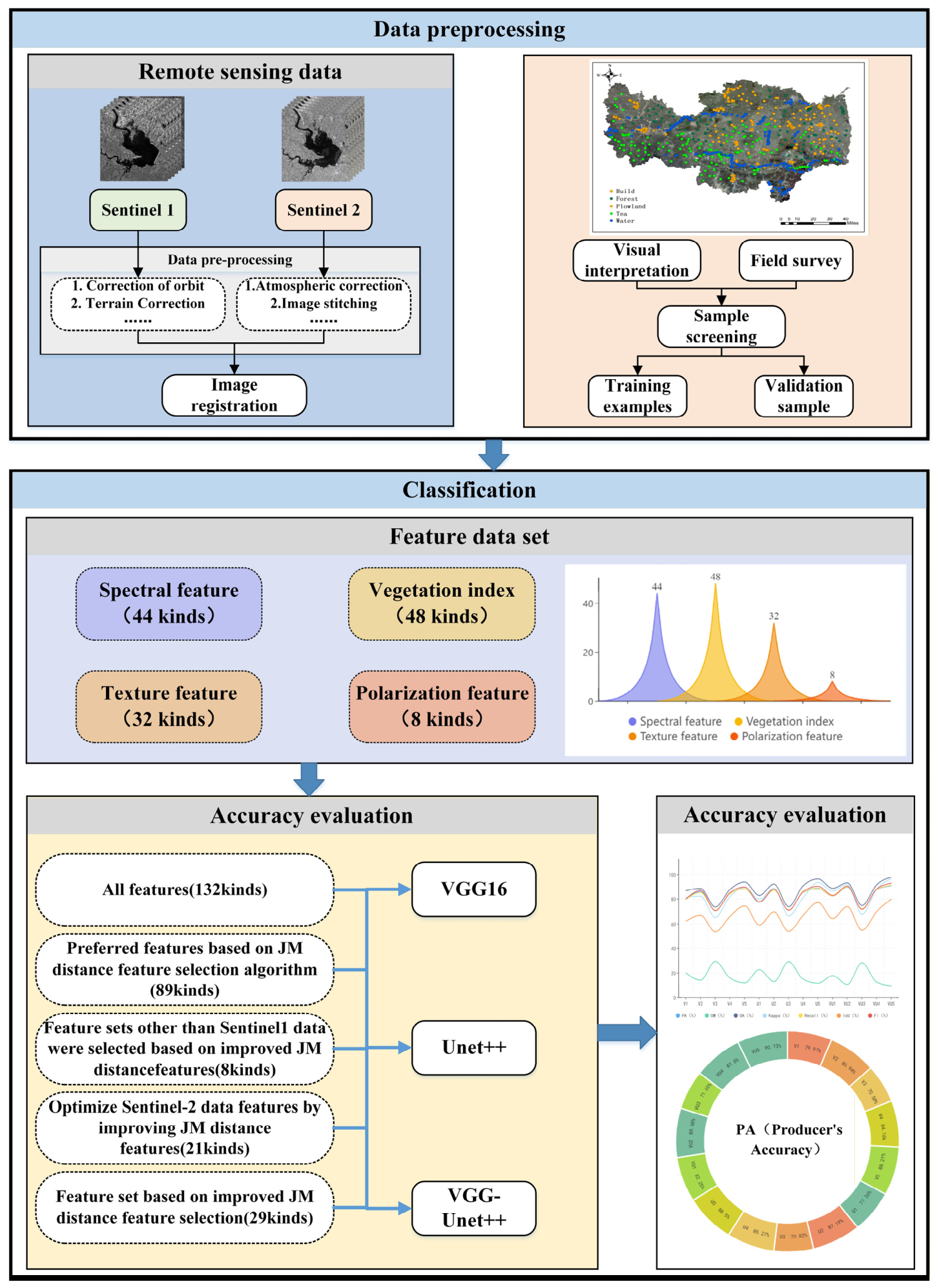
This study establishes a systematic methodological framework for the precise mapping of tea plantations in complex terrain. As illustrated in Figure 1, the workflow integrates multi-source feature engineering with optimized deep learning architectures, structured into four phases: (1) Data Preprocessing and Feature Extraction, where multi-temporal Sentinel-1 and Sentinel-2 imagery are synthesized to derive spectral, radar, and texture metrics; (2) Separability-Based Screening, utilizing the JM distance to isolate features with high discriminatory potential; (3) Redundancy Elimination, employing Pearson correlation analysis to prune highly collinear variables, ensuring a compact and efficient feature space; and (4) Deep Learning Classification, where three CNN architectures VGG16, UNet++, and a hybrid VGG16-UNet++ are trained for pixel-level segmentation.

3.1. Feature Set Construction

Based on the preprocessed Sentinel imagery, a multidimensional feature space comprising 132 variables was constructed to characterize the phonological dynamics and structural attributes of tea plantations. This feature set includes 44 spectral features directly extracted from Sentinel-2 bands, 48 vegetation index features calculated from established optical indices, 32 texture features obtained via Principal Component Analysis (PCA) on both optical and SAR data, and 8 polarization features derived from Sentinel-1 VV and VH backscatter coefficients. To facilitate reproducibility and systematic analysis, a standardized naming convention was applied to all variables. Detailed naming rules and feature descriptions are provided in

Table 4. Coding scheme and variable categories of the multi-temporal Sentinel-1/2 feature set, including spectral bands, vegetation indices, texture measures, and SAR polarization features.

Characteristic	Data
	May 2022	June 2022	August 2022	February 2023
B2	M1	J1	A1	F1
B3	M2	J2	A2	F2
B4	M3	J3	A3	F3
B5	M4	J4	A4	F4
B6	M5	J5	A5	F5
B7	M6	J6	A6	F6
B8	M7	J7	A7	F7
B9	M8	J8	A8	F8
B10	M9	J9	A9	F9
B11	M10	J10	A10	F10
B12	M11	J11	A11	F11
NDVI	M12	J12	A12	F12
EVI	M13	J13	A13	F13
RVI	M14	J14	A14	F14
DVI	M15	J15	A15	F15
NDWI	M16	J16	A16	F16
SAVI	M17	J17	A17	F17
NDVIre1	M18	J18	A18	F18
NDVIre2	M19	J19	A19	F19
NDVIre3	M20	J20	A20	F20
NDre1	M21	J21	A21	F21
NDre2	M22	J22	A22	F22
CIre	M23	J23	A23	F23
Mean	M24	J24	A24	F24
Variance	M25	J25	A25	F25
Entropy	M26	J26	A26	F26
Angular second moment	M27	J27	A27	F27
Correlation	M28	J28	A28	F28
Dissimilarity	M29	J29	A29	F29
Homogeneity	M30	J30	A30	F30
Contrast	M31	J31	A31	F31
VV	M32	J32	A32	F32
VH	M33	J33	A33	F33

Note: B2–B12 denote Sentinel-2 spectral bands; NDVI–CIre represent vegetation indices derived from optical imagery; Mean–Entropy denote texture features derived from PCA-transformed optical and SAR data; VV and VH represent Sentinel-1 polarization backscatter features. The prefixes M, J, A, and F indicate features derived from imagery acquired in May 2022, June 2022, August 2022, and February 2023, respectively.

.

3.2. Feature Optimization Strategy

High-dimensional feature spaces in remote sensing often contain irrelevant or redundant data, which can lead to the curse of dimensionality and impede the convergence of deep learning models [36]. To address this, we implemented a two-stage hybrid optimization strategy. First, the JM distance was calculated to screen for features with high class separability between tea plantations and other land cover. Second, to mitigate multicollinearity among the retained high-separability features, Pearson correlation analysis was applied to eliminate redundant variabiles. This process yielded a compact, low-redundancy feature subset optimized for classification.

The JM distance quantifies the separbility between two classes by measuring the average distance between their probability density functions [37]. It is calculated as:

$$JM=2\left(1-e^{-B_{ij}}\right)$$

(1)

where B_ij is the Bhattacharyya distance, which is defined as:

$$B_{ij}={\displaystyle \frac{1}{8}}{\displaystyle \frac{{(m_i-m_j)}^2}{{\delta }_i^2+{\delta }_j^2}}+{\displaystyle \frac{1}{2}}\ln \left({\displaystyle \frac{{\delta }_i^2+{\delta }_j^2}{2{\delta }_i{\delta }_j}}\right)$$

(2)

where JM is the JM distance between categories i and j; and are the means of feature vectors corresponding to categories m_i and m_j; and are the standard deviations of feature vectors corresponding to categories δ_i and δ_j. The value range of JM is [0, 2], and within this range, the larger the value of JM, the higher the degree of separation between categories. In this study, a JM distance threshold of JM ≥ 1.8 was applied to retain features with strong inter-class separability. Empirical analyses showed that lower thresholds preserved many weakly discriminative and redundant features, whereas more stringent thresholds removed bands providing complementary phenological and polarization information. Accordingly, JM ≥ 1.8 was selected, based on cross-validation, as a practical trade-off that maintains high inter-class separability while effectively controlling feature dimensionality, reducing the initial 132 features to 89 candidates enriched in red-edge, near-infrared, and texture descriptors.

To mitigate feature collinearity, Pearson correlation coefficients (P) were computed, and feature pairs with $\left|\mathrm{P}\right|>0.8$, a commonly accepted threshold indicating strong linear correlation were identified as redundant [38]. In each highly correlated pair, only one representative feature was retained to reduce multicollinearity. This Pearson-enhanced JM distance framework thus simultaneously maximizes inter-class separability and minimizes feature redundancy. The optimization objective is formalized as follows:

$$P={\displaystyle \frac{{\displaystyle {\sum }_{t=1}^n\left(X_t-\overline{X}\right)\left(Y_t-\overline{Y}\right)}}{\sqrt{{\displaystyle {\sum }_{t=1}^n{\left(X_t-\overline{X}\right)}^2}}\sqrt{{\displaystyle {\sum }_{t=1}^n{\left(Y_t-\overline{Y}\right)}^2}}}}$$

(3)

where $\overline{\mathrm{X}}$ and $\overline{\mathrm{Y}}$ denote the means of X and Y, and n is the number of samples.

For each highly correlated pair, only one representative feature was retained to reduce multicollinearity. Specifically, we calculated the mean JM distance of each feature across all class pairs and retained the feature with the higher mean JM value. When the difference in mean JM between the two features was negligible (less than 0.02), we preserved the feature with clearer biophysical interpretability for tea plantation discrimination (e.g., red-edge or phenology-sensitive indices) and discarded its counterpart. This deterministic rule avoids arbitrary or random removal and ensures that redundancy reduction is both statistically grounded and physically meaningful.

In practice, the procedure operates sequentially: (1) JM-based screening (JM ≥ 1.8) to preserve features with strong separability; and (2) Pearson-based pruning ($\left|\mathrm{P}\right|>0.8$) to eliminate redundant features according to the above rule. This JM-Pearson framework thus maximizes inter-class separability while controlling redundancy, without redefining the JM distance itself. The resulting compact subset (28 features; see Section 4.3) provides an efficient and reproducible input space for subsequent mapping experiments.

3.3. VGG16-UNet++ Hybrid Network Model

To achieve accurate yet efficient tea plantation mapping over large mountainous areas under limited pixel-level supervision, we adopt a VGG16–UNet++ hybrid segmentation architecture. Specifically, VGG16 provides a lightweight and well-conditioned encoder with mature ImageNet initialization [39], while UNet++ leverages nested skip pathways to preserve fine structures and strengthen multi-scale feature fusion [24,40]. This combination is well suited to narrow, terraced, and fragmented tea patches embedded in heterogeneous forest–cropland mosaics, where both global context and boundary fidelity must be retained. Compared with deeper backbones (e.g., ResNet/EfficientNet), VGG16 offers regular 3 × 3 convolutional blocks, stable optimization behavior, and mature pre-trained weights, providing a lightweight yet reliable encoder for multi-source Sentinel-1 and Sentinel-2 satellite data provided by the European Space Agency (ESA) while reducing architectural complexity and overfitting risk under limited labels and large-area inputs.

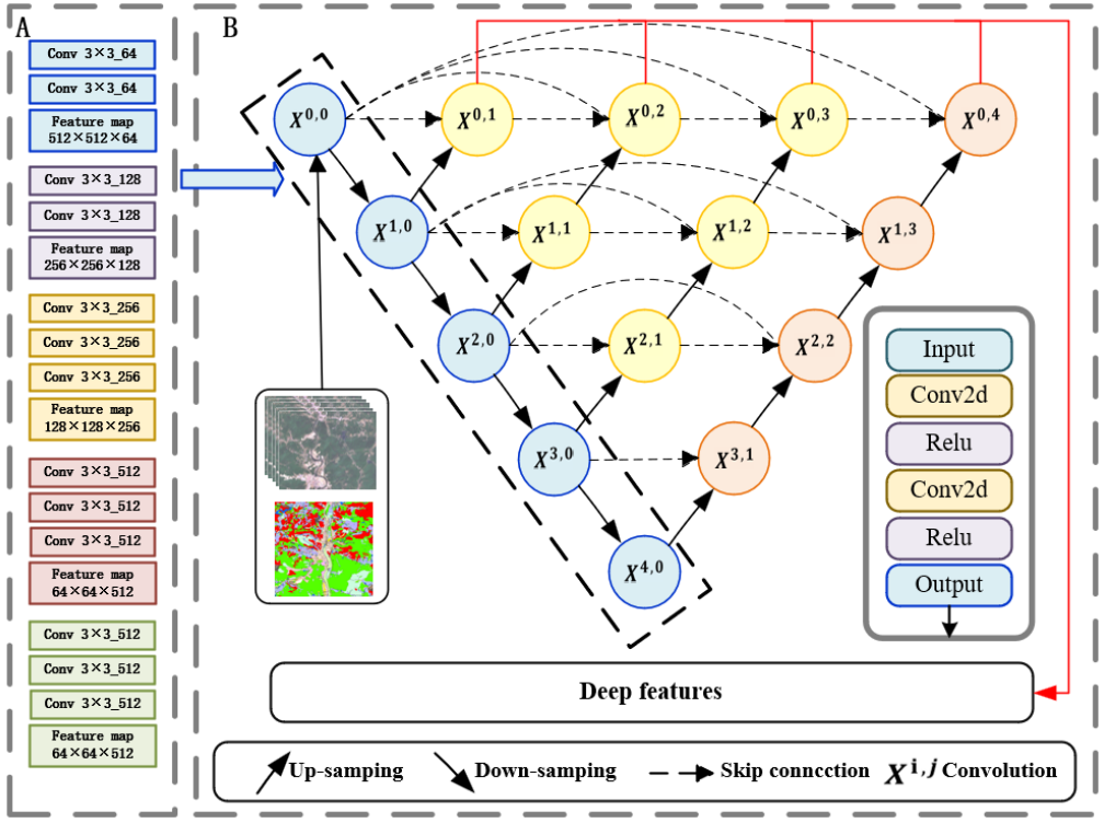
To address the channel mismatch between the multi-source feature stack (C > 3) and the ImageNet-pretrained VGG16 encoder (3-channel input), we prepend a lightweight 1 × 1 convolutional projection module that maps the H × W × C tensor to a three-channel pseudo-RGB representation via learnable linear combinations, enabling ImageNet initialization while retaining non-RGB predictors. The projection layer is trained from scratch, whereas the VGG16 encoder is initialized with ImageNet weights and jointly fine-tuned end-to-end with UNet++. As illustrated in Figure 2, the encoder comprises the first 13 convolutional layers of VGG16, using 3 × 3 kernels and channel widths of 64/128/256/512 with ReLU activations. Through successive pooling operations, the spatial resolution is reduced from 512 × 512 × C to 32 × 32 × 512, yielding compact high-level representations. The decoder progressively up-samples feature maps (bilinear interpolation) and performs dense skip fusion to reconstruct a 512 × 512 × K per-pixel probability map. Four-stage feature fusion combines encoder features with decoder up-sampled representations through cascaded skip connections, enabling precise pixel-wise segmentation for tea plantations in complex mountainous landscapes.

3.4. Experimental Design

This study utilized the TensorFlow 2.9.0 deep learning framework with Python 3.9.0 to implement three models: VGG16, UNet++, and the hybrid VGG16-UNet++ network. These models were designed to extract feature information from remote sensing data efficiently, supporting the tea plantation information extraction task. Model training was conducted on an NVIDIA GeForce RTX 3080 Ti GPU. Transfer learning with pre-trained model weights facilitated rapid convergence and improved the learning of target-specific features. After pre-training, the models were fine-tuned on domain-specific samples to optimize performance. Key hyperparameters for fine-tuning included 120 epochs, a batch size of 4, the Adam optimizer, and an initial learning rate of 0.0001. A learning rate decay mechanism was implemented, halving the learning rate when validation loss failed to decrease for three consecutive epochs. This dynamic adjustment improved convergence and mitigated overfitting, enhancing model efficiency and accuracy.

To rigorously assess the effectiveness of the two-stage JM distance and Pearson correlation-based feature selection strategy in reducing dimensionality, minimizing redundancy, and improving computational efficiency, a series of classification experiments were systematically designed. These experiments also aimed to benchmark the performance of the hybrid VGG16-UNet++ architecture for tea plantation mapping. To ensure a comprehensive evaluation, three deep learning architectures VGG16, UNet++, and the hybrid VGG16-UNet++ were systematically combined with six distinct feature subsets. This resulted in 18 experimental configurations, each representing a unique pairing of network model and feature strategy. For clarity and reference, all combinations were clearly labeled and are detailed in

Table 5. Classification experiment combination information table.

Features	VGG16	Unet++	VGG16-Unet++
A feature combination built on all features of Sentinel-1/2 image data (132 features)	V1	U1	VU1
Based on Sentinel-1/2 image data, JM distance feature selection algorithm is used to optimize the feature combination (89 features)	V2	U2	VU2
Feature combinations based on Sentinel-1/2 image data from June (33 features)	V3	U3	VU3
Feature combination based on Sentinel-1 image data polarization features (8 features)	V4	U4	VU4
Based on Sentinel-2 image data, the feature combination is constructed by the two-stage JM distance and Pearson correlation feature selection strategy (21 features)	V5	U5	VU5
Based on Sentinel-1/2 image data, the feature combination is constructed by the two-stage JM distance and Pearson correlation feature selection strategy (28 features)	V6	U6	VU6

.

3.5. Evaluation Metrics

To comprehensively assess the performance of the network model in remote sensing image classification, a set of evaluation metrics was employed, including Producer’s Accuracy (PA), User’s Accuracy (UA), Overall Accuracy (OA), Intersection over Union (IoU), and F1 Score (F1) [41]. The mathematical definitions of these metrics are presented below to ensure clarity and reproducibility.

$$PA={\displaystyle \frac{TP}{TP+FN}}$$

(4)

$$UA={\displaystyle \frac{TP}{TP+FP}}$$

(5)

$$OA={\displaystyle \frac{TP+TN}{TP+FN+FP+TN}}$$

(6)

$$IoU={\displaystyle \frac{TP}{TP+FP+FN}}$$

(7)

$$F1={\displaystyle \frac{2\times PA\times UA}{PA+UA}}$$

(8)

In this context, TP (True Positive) referred to the number of pixels correctly classified as belonging to a certain category. FP (False Positive) denoted the number of pixels incorrectly identified as belonging to the category. FN (False Negative) indicated the pixels that belonged to the category but were not classified as such by the model.

3.6. Ecological Indicators and Spatial Risk Metrics

To quantify landscape risk, we start from the K-class land-cover map predicted by the segmentation network and construct a consistent tea–forest analysis domain by retaining only the tea and forest labels while masking all other categories (water, built-up, cropland) as NoData. We then integrate three layers for metric computation: (1) the derived tea–forest domain mask, (2) a DEM-based slope raster, and (3) a 1 km × 1 km aggregation grid. The segmentation network produces a K-class land-cover map; however, ecological-risk computation retains only the tea and forest classes. All remaining categories (e.g., water, built-up, cropland) are masked out so that the exposure and interface metrics are computed on a consistent tea-forest domain across all experiments. All layers are projected to the common coordinate reference system (CRS), co-registered and snapped to a common grid; the classification is resampled by nearest neighbor, the slope by bilinear interpolation. Pixels flagged as NoData (and water, where available) are masked.

Slope is computed from the DEM using the Horn operator and resampled to the classification grid. For quantile-based thresholding and statistical baselines, valid 1-km grids are defined as grid cells that contain at least one tea or forest pixel after masking non-tea/non-forest classes; fully masked cells are excluded from the baseline distribution. For policy-relevant thresholds $\mathsf{\theta }=\left\{10°,12°,15°,20°,25°\right\}$, we report the area of tea occurring on slopes steeper A_θ than θ and its share of the total tea extent P_θ:

$$A_{\theta }={\displaystyle \sum _{p\in tea}1\left\{slope\left(p\right)\ge \theta \right\}}·{\displaystyle \frac{s^2}{{10}^6}}$$

(9)

$$P_{\theta }=100\times {\displaystyle \frac{A_{\theta }}{A_{tea}}}\left(\%\right)$$

(10)

where s is the pixel size (m), A_tea is total tea area (km²), and 1$\left\{\mathrm{s}\mathrm{l}\mathrm{o}\mathrm{p}\mathrm{e}\left(\mathrm{p}\right)\ge \mathsf{\theta }\right\}$ is the indicator function. Grid-level metrics A_θ,i, P_θ,i are computed for each 1-km cell i to map local concentration.

Boundary length is estimated on the raster map under 8-neighbor (queen) connectivity with diagonals included. For every tea pixel adjacent to forest, orthogonal contacts contribute length s, and diagonal contacts contribute $\sqrt{2}\mathrm{s}$. The global interface length and the grid-level density are:

$$L={\displaystyle \sum _{e\in E_{tea-forest}}l\left(e\right)}\left(\mathrm{m}\right)$$

(11)

$$D_i={\displaystyle \frac{L_i}{A_i}}\left(\mathrm{m}/\mathrm{k}{\mathrm{m}}^2\right)$$

(12)

With A_i = 1 km². To suppress speckle, connected components <9 pixels are removed from both tea and forest prior to adjacency counting. The 8-neighbor rule and diagonal inclusion are fixed across analyses for comparability.

To avoid arbitrary cut-points, hotspots are defined by empirical quantiles of the study-wide distribution over valid 1-km grids for each indicator: Q90 (90th percentile) denotes high exposure/density and Q75 (75th percentile) denotes moderate-to-high exposure. For operational prioritization, we further adopt an integrated decision rule to flag composite hotspots: a 1-km grid is prioritized when tea–forest interface density is high and steep-slope tea exposure is at least moderate-to-high, i.e., Di ≥ Q90 (D) and P_10°,i ≥ Q75(P_10°), where P_10°,i denotes the within-grid proportion of tea on slopes ≥ 10°. We explicitly report pixel size, CRS, connectivity (8-neighbour), diagonal handling (included), and minimum patch size (9 px), grid size (1 km), and the five slope thresholds.

4. Results

4.1. Network Model Training and Loss Analysis

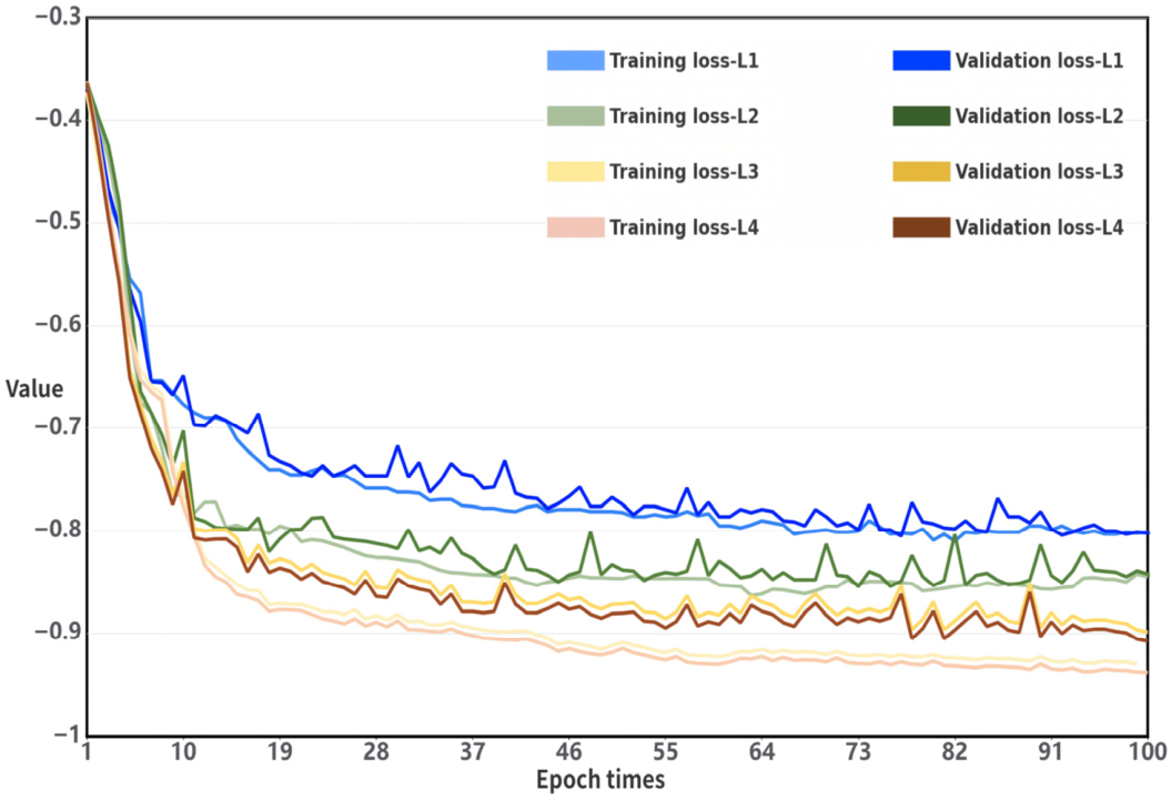
The VGG16-UNet++ network was trained using the constructed training and validation datasets under consistent hyperparameter settings. During training, four deeply supervised decoder outputs at different depths (L1, L2, L3, L4) were monitored to evaluate convergence behavior and representation quality. The corresponding training and validation loss curves are shown in Figure 3. The loss curves indicate that all four outputs exhibit rapid loss reduction in the early training stage, followed by gradual stabilization, with no obvious signs of overfitting. Although the L3 branch shows a local trough near the late training stage (around epoch 100), this fluctuation is transient and remains within a limited range, without indicating instability or divergence. Among them, L4 (the deepest decoder output) consistently achieves the lowest and most stable validation loss, demonstrating that the deepest supervision branch, which fully integrates high-level semantic features and multi-scale contextual information through nested skip connections, provides the most discriminative and robust representation. Based on this observation, L4 is selected as the final output for subsequent tea plantation mapping and accuracy assessment.

4.2. JM Distance Feature Selection Results

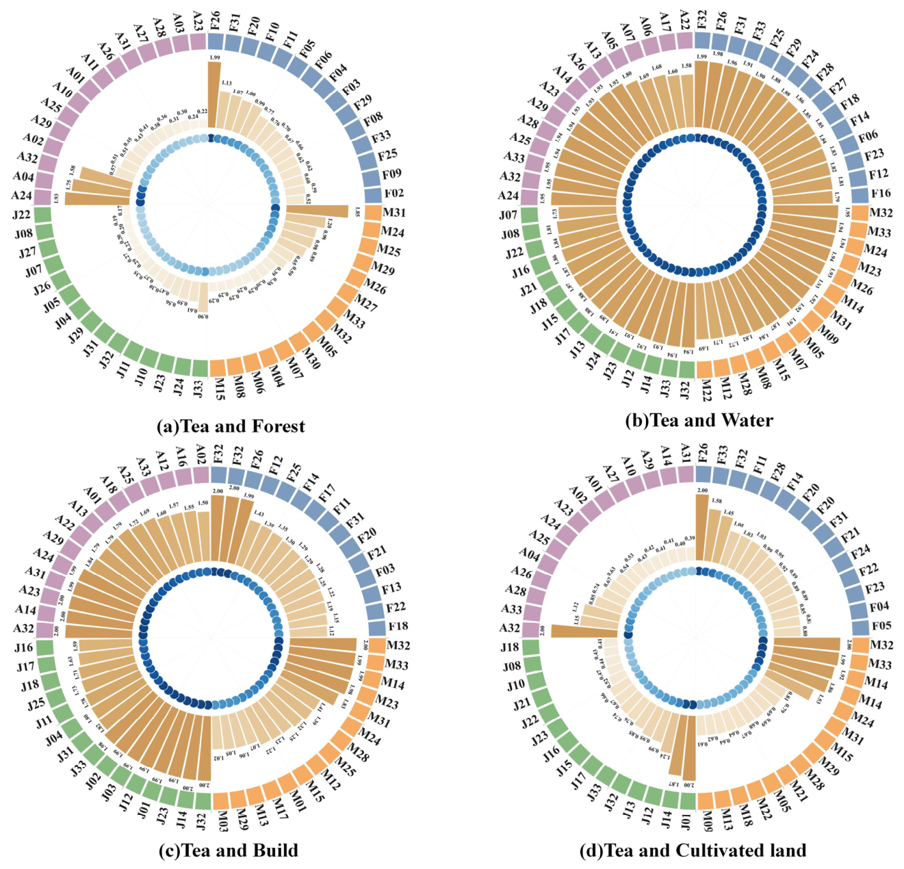
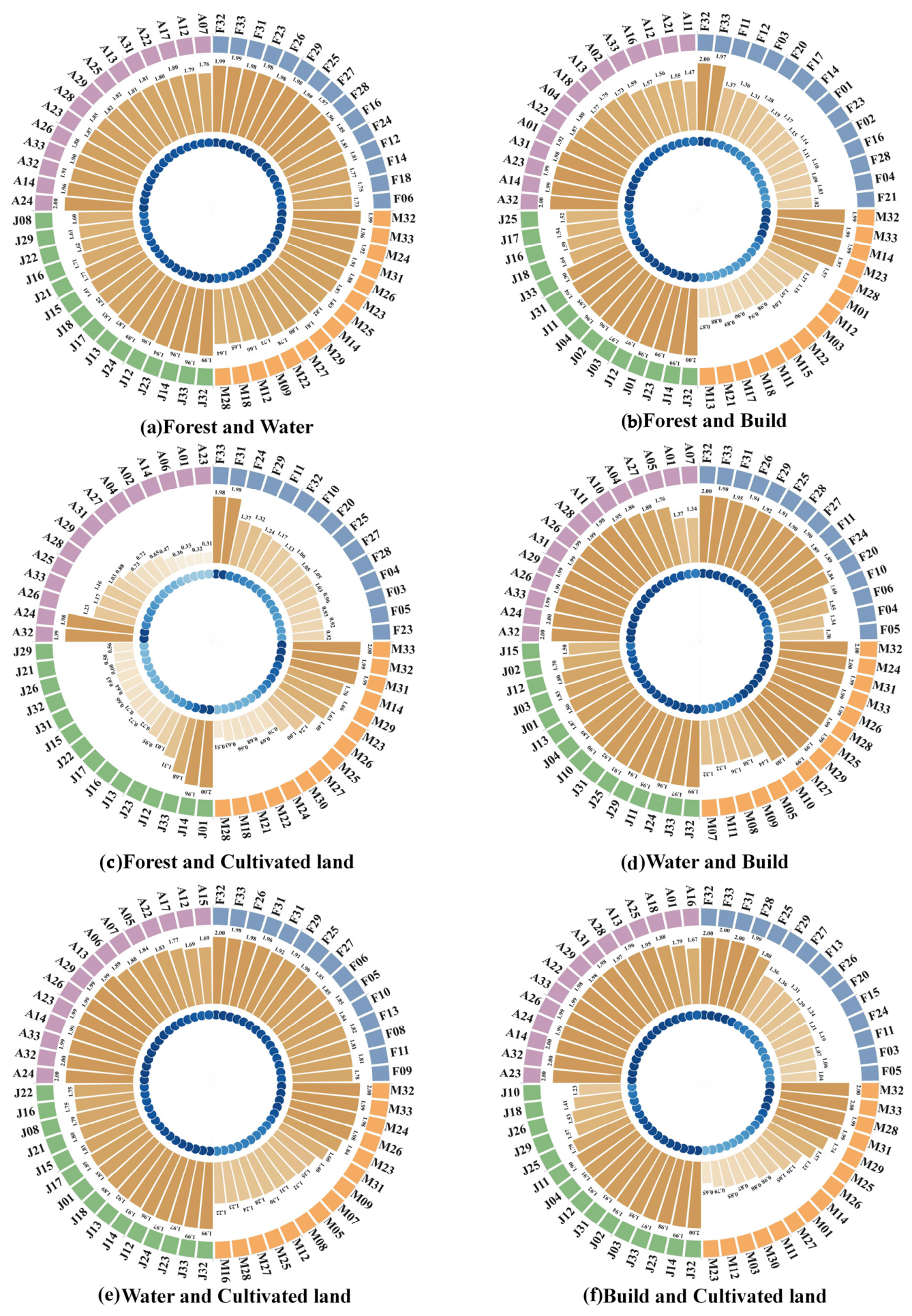
Following the JM-based screening procedure described in Section 3.2, we evaluated inter-class separability across all 132 candidate variables (spectral, vegetation index, texture, and polarization) and retained 89 features for subsequent analysis. This process resulted in the selection of 89 features exhibiting strong separability across various land cover types. The pairwise JM distance distributions among ten typical class combinations such as tea plantations vs. forest, water, and cultivated land are presented in Appendix A Figure A1 and Figure A2. Specifically, class pairs such as tea plantation vs. water body (61 features), forest vs. water body (43 features), and water body vs. cultivated land (40 features) exhibited the highest number of features exceeding the JM threshold, indicating strong spectral and structural dissimilarity. In contrast, pairs such as tea plantation vs. forest (3 features) and tea plantation vs. cultivated land (7 features) demonstrated limited separability, reflecting substantial spectral overlap and potential classification confusion. Moderate levels of separability were observed for tea plantation vs. built-up area (23 features), water body vs. built-up area (23 features), forest vs. cultivated land (9 features), and built-up area vs. cultivated land (21 features), indicating varying degrees of complexity in inter-class discrimination.

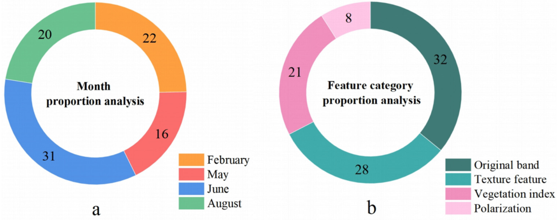
As illustrated in Figure 4a, features derived from June accounted for the largest proportion of selected variables (31 features, 34.8%), likely due to the strong phenological contrast during the peak tea canopy development stage. February contributed the second-highest number (20 features, 22.5%), benefiting from the distinct spectral response of evergreen tea relative to dormant vegetation during the winter season. Figure 4b further indicates that spectral features, particularly those from the red-edge and near-infrared bands, dominated the selected feature set, with 68% exceeding the JM threshold. Additionally, texture features, notably those capturing image contrast (e.g., M31), also exhibited high discriminative capacity, with 75% surpassing JM ≥ 1.8. These results underscore the complementary importance of spectral and spatial information in enhancing land cover class separability within complex agro-ecological environments.

4.3. Pearson-Correlation Pruning Results

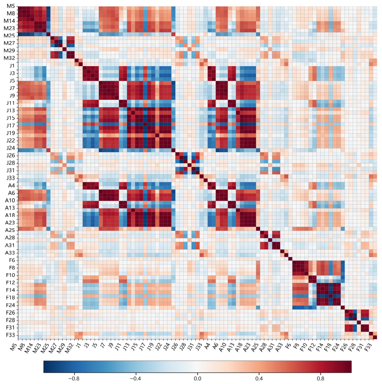
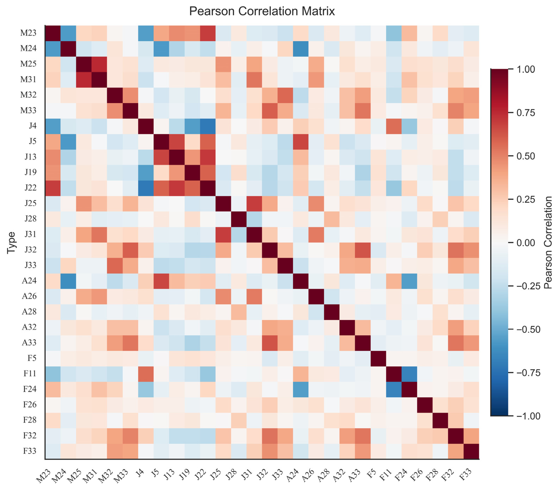
Following the Pearson-correlation pruning described in Section 3.2, the JM-retained subset was reduced from 89 to 28 decorrelated predictors (−68.5%), improving computational efficiency while suppressing redundancy and retaining complementary information for classification. Figure 5 depicts the correlation matrix of the original 89 features, clearly illustrating the presence of strongly correlated feature clusters that are subsequently mitigated by the pruning step.

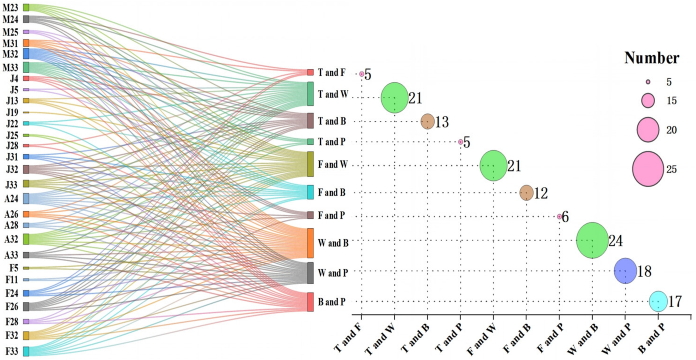
The retained features were further assessed for their class separability across all pairwise land cover combinations, as shown in Figure 6. The tea plantation-forest and tea plantation-cultivated land pairs exhibited the fewest separable features (n = 5), indicating limited spectral and structural divergence between tea plantations and spectrally similar vegetated backgrounds. This similarity likely arises from overlapping phenological phases, comparable canopy architectures, and similar red-edge reflectance responses. In contrast, the greatest number of separable features was observed for water body-built-up area (n = 24), forest-water body (n = 21), and tea plantation-water body (n = 21), reflecting stronger inter-class differentiation. These distinctions can be primarily attributed to differences in surface moisture content, spectral response characteristics-particularly in the near-infrared and shortwave infrared regions-and landscape texture complexity. This pairwise analysis provides deeper insights into the sensitivity of selected features to specific land cover transitions, and serves as a foundation for developing more targeted and robust classification strategies in heterogeneous landscapes.

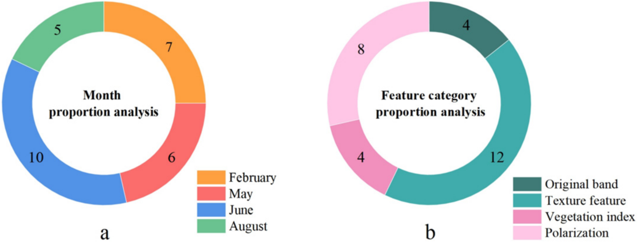
Further temporal and categorical analyses of the 28 selected features revealed clear distributional patterns (Figure 7). Temporally, the majority of retained features were derived from June (n = 10), corresponding to the phenological peak of tea canopy development and maximal inter-class vegetation contrast. February and May contributed 7 and 6 features, respectively, capturing seasonal transitions and enhancing the characterization of background variability and senescent vegetation signals. From a categorical perspective (Figure 7b), texture features represented the largest proportion (n = 12), followed by spectral bands (n = 8), polarization features (n = 4), and vegetation indices (n = 4). The dominance of texture-based features-particularly low-correlation descriptors such as entropy (e.g., M26, $\left|\mathrm{P}\right|\le 0.5$) highlights their critical role in capturing spatial heterogeneity and boundary complexity within fragmented agro-ecological landscapes. These findings underscore the added value of spatial-textural information in improving land cover discrimination in high-resolution remote sensing applications. As shown in Figure 8, the final 28-feature correlation matrix exhibits no pronounced high-correlation clusters, confirming effective redundancy suppression and improved complementarity among retained predictors.

4.4. Classification Results

To assess the impact of different feature selection strategies and model architectures on tea plantation classification performance, a total of eighteen experimental configurations were evaluated. Classification outcomes were quantitatively assessed using standard performance metrics, including PA, UA, OA, IoU and F1. A comprehensive summary of the results is presented in

Table 6. Classification performance across different experimental configurations.

Experimental Combination	PA (%)	UA (%)	OA (%)	IoU	F1
V1	79.97	79.67	86.70	0.6202	0.7982
V2	85.94	85.09	88.53	0.6680	0.8551
V3	73.54	73.65	75.42	0.5539	0.7359
V4	70.58	70.56	73.23	0.5336	0.7057
V5	84.16	84.25	87.65	0.6575	0.8420
V6	88.21	88.27	93.80	0.7422	0.8824
U1	77.26	77.78	82.70	0.5887	0.7752
U2	87.19	87.15	92.10	0.6934	0.8717
U3	72.63	72.73	74.24	0.5468	0.7268
U4	70.82	70.84	73.56	0.5370	0.7083
U5	85.27	85.43	90.85	0.6686	0.8535
U6	88.50	88.85	96.35	0.7701	0.8867
VU1	82.25	82.32	88.58	0.6410	0.8228
VU2	89.58	89.83	93.21	0.7372	0.8970
VU3	75.24	75.17	78.68	0.5682	0.7520
VU4	71.65	71.81	74.48	0.5455	0.7173
VU5	87.60	87.71	91.52	0.6964	0.8765
VU6	90.73	91.14	97.82	0.7968	0.9093

. Given that tea plantation identification was the primary objective of this study, PA was designated as the key evaluation metric to reflect class-specific accuracy.

The baseline configurations (V1, U1, VU1), which employed the complete 132-dimensional feature set without any selection, yielded only moderate classification performance (e.g., VU1: PA = 82.25%). This likely reflects redundancy/noise in the full feature set. By incorporating the traditional JM distance algorithm (V2, U2, VU2), classification accuracy improved notably across all model architectures, thereby validating the effectiveness of separability-based feature filtering in enhancing model discriminability. The highest performance was attained by the VU6 configuration, which combined the VGG16-UNet++ hybrid network with a 28-dimensional feature subset derived via the proposed Pearson-enhanced JM distance method. This setting achieved a PA of 90.73%, while reducing the average feature correlation coefficient (P) from 0.72 to 0.31-indicating successful suppression of feature redundancy without compromising discriminative capability. Across all models, the adoption of the optimized feature subset consistently enhanced classification accuracy: V6 outperformed V1 by 8.2%, U6 surpassed U1 by 11.2%, and VU6 improved upon VU1 by 8.5%. Configurations utilizing radar-only features (V4, U4, VU4) exhibited lower performance compared to multi-source fusion strategies, though they still outperformed the single-temporal feature setups (VU3: PA = 75.24%). Furthermore, optimized feature sets derived solely from Sentinel-2 data (VU5) performed slightly below the VU6 configuration, supporting the value of multi-source and multi-temporal integration.

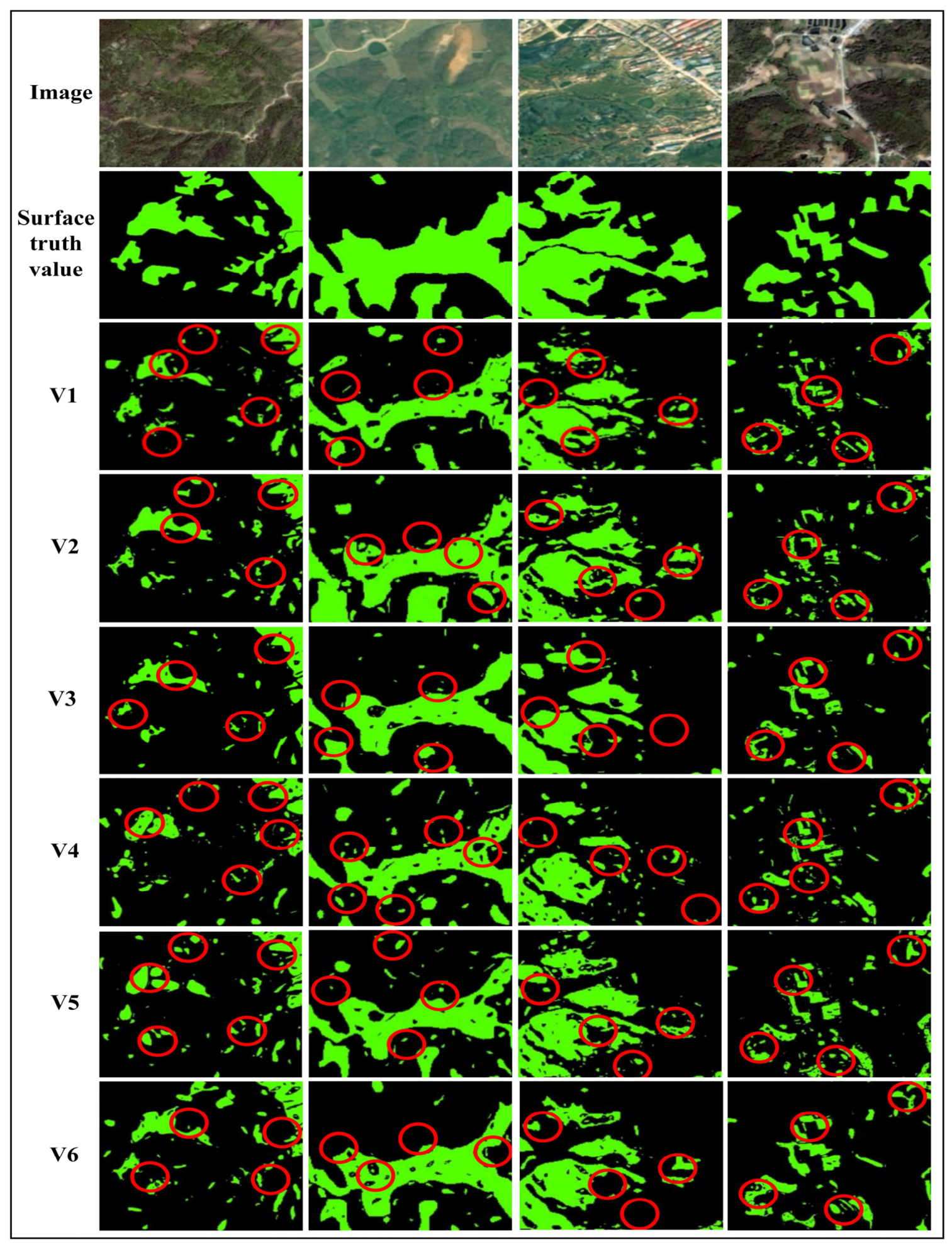
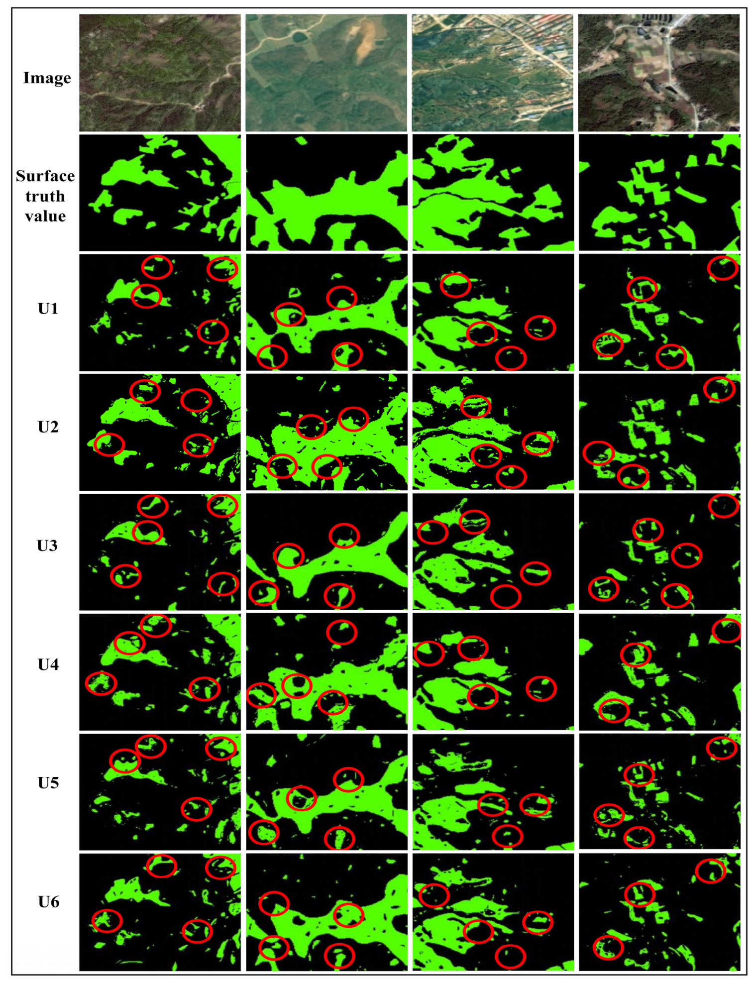
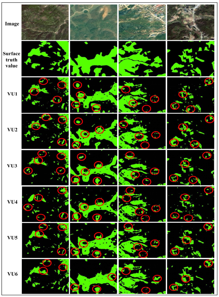
Visual comparisons across feature settings are provided for each architecture, with Figure 9 showing the hybrid VGG16–UNet++ results (VU1–VU6), Appendix A Figure A3 showing the VGG16-only results (V1–V6), and Appendix A Figure A4 showing the UNet++-only results (U1–U6). In Figure 9, the baseline hybrid setting (VU1) produces noticeably fragmented tea patches and scattered speckle-like artifacts, particularly in the red-circled regions where confusion with adjacent forests/croplands is most evident. With separability-based filtering (VU2) and further redundancy pruning (VU6), tea patches become progressively more compact and spatially continuous, and the number of isolated false fragments is reduced. The radar-only setting (VU4) tends to miss portions of tea patches and yields discontinuous outputs in several circled areas, whereas Sentinel-2–only optimized features (VU5) recover more tea extent but still show residual local confusion compared with VU6. Appendix A Figure A3 indicates that VGG16-only maps (V1–V6) generally exhibit coarser boundaries and more scattered isolated fragments, even though feature optimization from V1 to V6 visibly improves patch coherence. Appendix A Figure A4 shows that UNet++ only outputs (U1–U6) are typically smoother and more regionally connected, but can display slight over-smoothing in some narrow tea strips, relative to the hybrid results. Overall, the visual evidence in Figure 9 and Appendix A Figure A3 and Figure A4 is consistent with Table 6, supporting that the proposed JM–Pearson feature subset and multi-source fusion lead to more stable and visually coherent tea plantation maps. Among the five land-cover categories, tea plantations are generally easier to distinguish from water bodies and built-up areas, whereas confusion is more likely to occur with forest and, to a lesser extent, cultivated land. Although cultivated land typically shows stronger seasonal variability than tea plantations, local misclassification may still occur in fallow fields, mixed vegetation patches, or fragmented plots adjacent to tea plantations, especially under complex terrain and shadow conditions.

4.5. Ecological Indicators and Spatial Risk Patterns

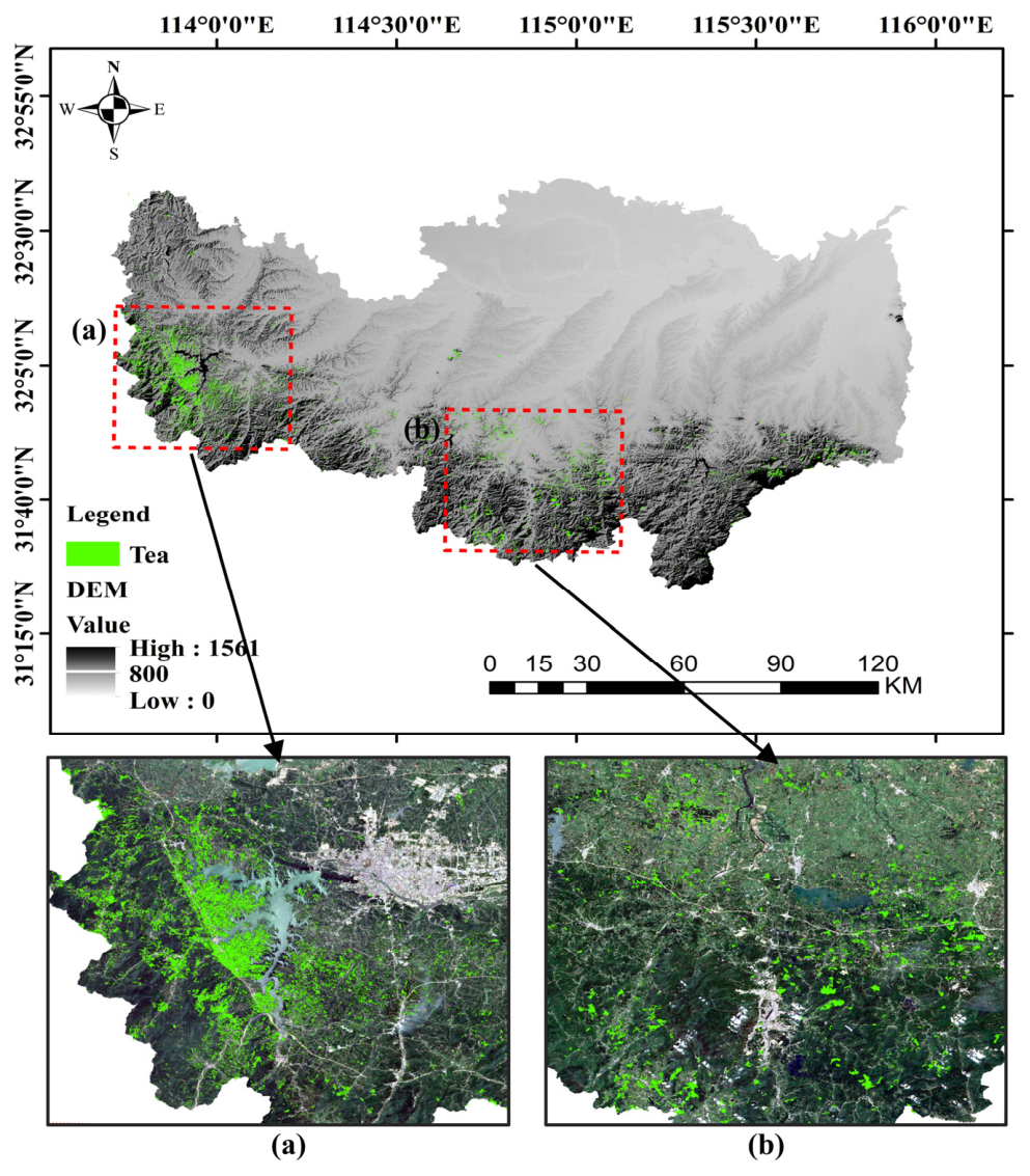
Using the optimal VU6 configuration, we generated a wall-to-wall map of tea plantations for Xinyang City and draped it over the DEM to visualize topographic context (Figure 10). Tea plantations occupy 1373.93 km² of the municipal territory and are predominantly concentrated on mid- to low-mountain hillslopes, with conspicuous alignments along forest margins, valley sidewalls, and riparian/reservoir buffers. According to the official statistic of 1440 km² for Xinyang, our mapped extent is 4.6% lower. The MMU-based post-processing (removing connected components smaller than 9 pixels) may additionally remove a limited number of fragmented micro-patches near forest edges, thereby slightly reducing the mapped total area. Overall, the spatial arrangement is consistent with terrain-controlled siting and proximity to forest margins, where microclimate, moisture availability, and access constraints jointly shape planting decisions.

Insets (a) and (b) in Figure 11 illustrate two representative concentration areas over very-high-resolution imagery. At these locations, tea patches form elongated, terrace-like strips that intensify tea-forest and tea-cropland interfaces and aggregate around fragmented forest patches. The resulting edge-rich mosaics improve separability relative to spectrally similar backgrounds in the VU6 product while revealing interface geometries that are pertinent to ecological risk (e.g., edge effects and downslope connectivity).

To further visualize the actual ecological conditions of tea plantations under different slope thresholds and supplement field survey evidence,

Table 7. Slope Thresholds, Quantitative Characteristics and Field Observations of Tea Plantations in Xinyang City.

Slope Threshold	Tea Plantation Area (km2)	Proportion of Total Tea Plantation Area (%)	Ecological Risk Correlation
10°	546.00	39.74	Distributed in zonal pattern on gentle slopes, complete terrace structures, soil surface covered with litter, slight erosion, standardized field management.
12°	408.33	29.72	Transition from gentle to steep slopes, uneven terrace slopes, relatively loose soil, slight rill erosion traces visible in rainy season.
15°	260.91	18.99	Concentrated at forest edges, narrow terraces, thin soil layer, signs of terrace ridge collapse in some areas, obvious forest fragmentation.
20°	117.75	8.57	Steep and long slopes, narrow terraces, erosion-prone soil, certain degree of surface exposure, significant runoff traces in rainy season, vulnerable terrace ridges.
25°	40.94	2.98	Distributed on south-facing steep slopes, partial lack of terrace protection, shallow soil layer, relatively high rock exposure, signs of rill erosion and small landslides.
10°	546.00	39.74	Distributed in zonal pattern on gentle slopes, complete terrace structures, soil surface covered with litter, slight erosion, standardized field management.

summarizes the slope thresholds, quantitative areas, proportions, and corresponding field observation characteristics. Based on the field survey in December 2022 (covering 15 tea plantation sample points), the field observations focus on terrain structure, soil conditions, erosion traces, and the spatial relationship between tea plantations and forests, which mutually confirm with the quantitative data above and provide concrete support for subsequent ecological risk assessment.

All quantile thresholds and statistical baselines reported in

Table 8. Ecological Indicator Thresholds at the 75th and 90th Percentiles (Statistical Baseline: Valid 1-km Grids in Xinyang).

Indicator	Unit	Q75	Q90
Steep-slope tea proportion (≥10°)	%	35.24	61.52
Tea-forest interface density (8-neigh)	mkm−2	0	4.09
Tea-forest interface density (4-neigh)	mkm−2	0	1.38
ΔD = D(8n) − D(4n)	mkm−2	0	2.69

are computed over valid 1-km grids, as defined in Section 3.6. Specifically, for tea-forest interface density, the 8-neighbour Q90 threshold (4.09 m/km²) is established as the primary regulatory benchmark, whereas the 4-neighbour Q90 threshold (1.38 m/km²) functions as a supplementary validation metric to mitigate biases arising from definitional variations. For the proportion of steep-slope tea plantations (≥10°), the Q75 value of 35.24% denotes that 75% of tea-bearing grids exhibit a steep-slope proportion lower than this threshold, while the Q90 value of 61.52% serves as the critical threshold for high ecological exposure. The integrated decision rule (tea-forest interface density ≥ Q90 and steep-slope tea proportion ≥ Q75) facilitates the prioritization of ecological risk hotspots, providing a standardized basis for targeted environmental surveillance and ecological restoration initiatives.

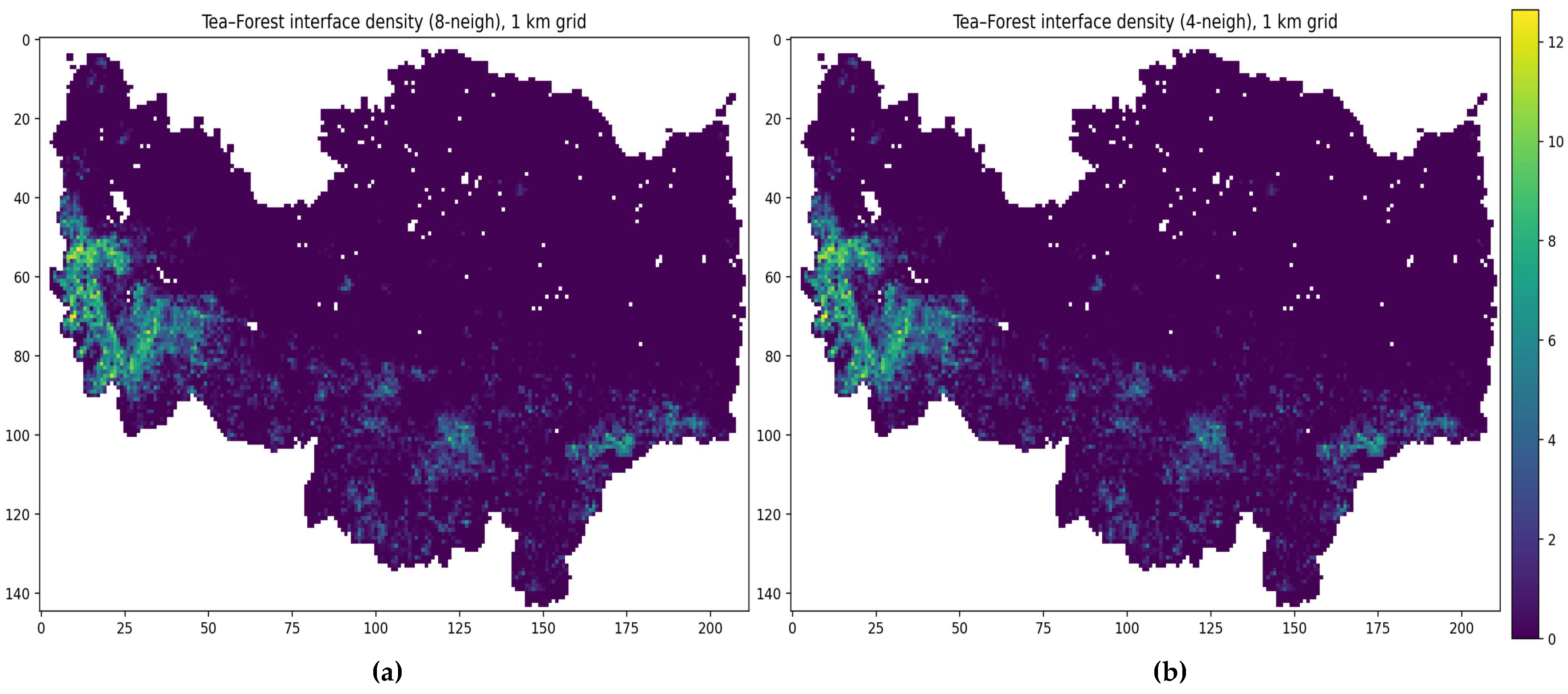
Combined with the field characteristics in Table 7, it can be seen that the erosion risk of steep-slope tea plantations is positively correlated with the degree of forest fragmentation, a pattern further verified in the subsequent spatial distribution of tea–forest interface density. Using the VU6 map aligned in WGS 84/UTM 50N, we quantified ecological sensitivity at landscape scale. Under 8-neighbour connectivity (diagonals included), the tea-forest interface length reaches 33,660 km, indicating pronounced edge prevalence and fragmentation. After grid-normalisation to 1 km × 1 km (D_i = L_i/A_i), units mkm⁻²), high-density cells cluster in belts and patches along the southern mountain-hill transition and major forest margins, closely co-locating with tea concentrated on steep terrain (Figure 11a). A parallel calculation with 4-neighbour connectivity confirms the same hotspot structure, with only expected differences along oblique/terraced boundaries (Figure 11b), demonstrating that hotspots are pattern-driven rather than definition-driven.

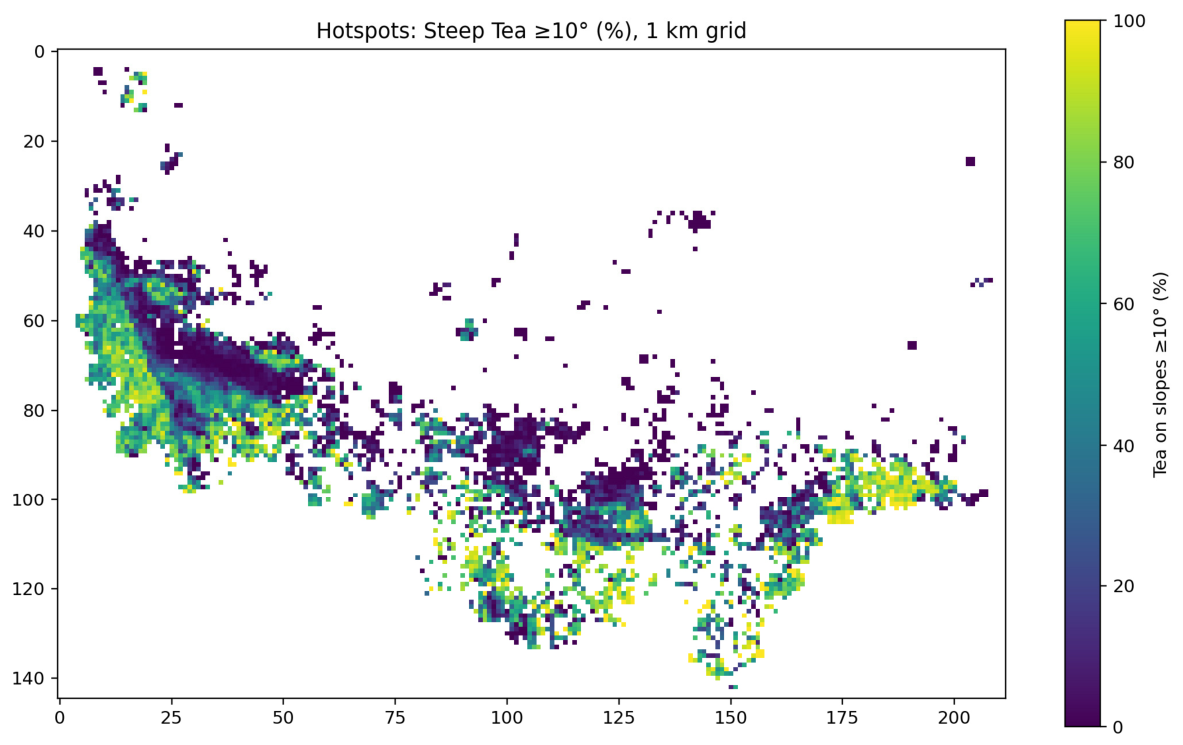
For steep-slope exposure, five thresholds θ = 10°/10°/12°/15°/20°/25° yield the expected monotonic decline: at 10°, A_10° = 546.00 km² and P_10° = 39.74%; at 25°, A_25° = 40.94 km² and P_25° = 2.98%. At 1-km resolution, cells with high P_10° markedly co-locate with cells of high interface density D_i, forming strings of hotspots along windward slopes, valley sides, and forest edges (Figure 12). This co-occurrence implies that slope-process sensitivity (erosion/landslide) and edge-effect pressure (fragmentation/microclimate/disturbance) overlap spatially, supporting priority regulation where high D_i × high P_θ,i conditions coincide.

Statistically, D_i is right-skewed, with upper quantiles contributing a disproportionate share of the total interface length, while P_10° is strongly conditioned by relief. An operational prioritisation rule naturally follows: patrol composite hotspots where D_i ≥ Q90 and P_10° ≥ Q75. Using 8-neighbour as the primary reporting convention and 4-neighbour as a methodological check provides a built-in robustness test without extra data cost. In short, interface density diagnoses structural fragmentation, whereas steep-slope exposure diagnoses process sensitivity; their spatial coupling yields actionable ecological-risk guidance.

5. Discussion

5.1. Comparative Insights Across Models

The hybrid VGG16-UNet++ network demonstrated clear superiority over the standalone VGG16 and UNet++ models in both classification accuracy and spatial coherence. Specifically, it achieved the highest PA of 90.73%, outperforming its counterparts by over 8% in PA. This gain is mainly due to combining VGG16’s robust pre-trained encoder for stable feature extraction from Sentinel-1/2 inputs with UNet++’s multiscale skip connections for joint context–detail fusion. The hybrid design reduces boundary confusion (especially tea vs. spectrally similar forest/cropland) and better preserves narrow, fragmented, terraced tea parcels in complex mountain mosaics. Beyond the quantitative metrics, the map-level comparisons help explain how the hybrid architecture improves spatial quality. Figure 10 reports the local extraction results produced by the VGG16–UNet++ model under different feature-set settings (VU1–VU6), while Appendix A Figure A3 and Figure A4 provide the corresponding results of the VGG16-only baselines (V1–V6) and the UNet++-only baselines (U1–U6), respectively. Under matched feature inputs, VGG16-only outputs tend to show higher patch fragmentation and local noise, whereas UNet++-only outputs are generally smoother and more contiguous but may mildly over-smooth tea–forest transitions, weakening thin terrace edges. The hybrid model mitigates both failure modes by retaining sharper boundaries while reducing fragmentation, which is particularly advantageous in shadowed or topographically distorted mountain mosaics. These findings are consistent with the principles underlying feature pyramid and multi-scale representation networks, which emphasize the value of multiscale fusion in capturing hierarchical patterns. Moreover, the hybrid approach aligns with emerging best practices in semantic segmentation for agricultural landscapes [33], demonstrating robust generalization in complex, fragmented terrains. In addition, the observed gains are strengthened by the JM–Pearson feature selection, which suppresses collinearity among multi-source predictors and makes the fused feature space more stable for dense multi-scale decoding.

5.2. Efficacy of Feature Selection Strategies

Feature selection plays a pivotal role in remote sensing classification, particularly under high-dimensional multi-source inputs. In this study, the sequential JM–Pearson filter described in Section 3.2 outperforms both the full-feature configuration and the JM-only scheme. This procedure achieves a 78.8% reduction in feature dimensionality (from 132 to 28 features) while maintaining or improving classification accuracy. Rather than introducing a new separability metric, it pragmatically integrates two well-established criteria to preserve highly discriminative features and suppress collinearity, which is particularly suitable for complex tea plantation landscapes. When combined with the hybrid VGG16-UNet++ network, the streamlined 28-dimensional subset consistently yields the best classification metrics, indicating that performance gains arise from a better-structured and more robust feature space. Compared with conventional JM-only approaches that focus solely on global class separability, the JM–Pearson strategy additionally controls redundancy among predictors, hereby alleviating feature collinearity and mitigating overfitting common challenges in hyperspectral and fusion-based remote sensing applications. Related studies employing mutual information or Relief have demonstrated the benefits of discriminative feature ranking [42], and the present work extends this line of research by providing a simple, deterministic, and reproducible JM-Pearson framework tailored to mountainous tea plantation mapping.

5.3. Role of Multi-Source and Multi-Temporal Fusion

Feature-importance profiling and controlled comparisons consistently indicate that the proposed multi-temporal strategy yields measurable gains in tea plantation mapping. Among the four phases, June-derived predictors contribute the largest share (35.7%), followed by February (25.0%), with May (21.4%) and August (17.8%) providing additional support. This contribution pattern implies that June and February capture the dominant discriminative signal, whereas May and August supply complementary temporal constraints that enhance phenological consistency and suppress class confusion. Taken together, the four phases constitute a robust phenological basis for tea/non-tea separation.

Architecture-matched experiments further corroborate this finding. Using VGG16–UNet++ as a representative backbone, the June-only setting (VU3) already reproduces the major tea distribution, while the four-phase multi-source setting coupled with two-stage feature selection (VU6) yields higher tea-class PA, UA, IoU, and F1, and substantially reduces the false assignment of forests and croplands to tea (Table 6). These results demonstrate that February, May, and August provide non-redundant corrective information beyond a single peak-growth snapshot.

The observed gains are mechanistically consistent with phenological complementarity. In February (winter dormancy), evergreen tea exhibits pronounced texture and SAR backscatter contrast relative to deciduous or senescent vegetation, improving the detection of persistent tea patches. In May (spring flush/early growth), canopy restructuring and management-induced signals increase spectral–textural distinctiveness, reducing confusion with early vegetation and bare soil. June corresponds to peak canopy development, when red-edge/NIR responses and vegetation indices are maximized, making it the primary window for separating tea from forests, croplands, and built-up land. In August (autumn tea with vigorous understory growth), cross-date consistency checks with earlier phases help retain stable tea signatures while filtering seasonal crops and transient covers. By integrating these stages, discrete observations are transformed into a temporal phenological signature, which amplifies cumulative contrast while reducing sensitivity to illumination variability, terrain shadowing, and local disturbances—thereby improving robustness in rugged and heterogeneous landscapes.

From a sensor-fusion perspective, SAR–optical complementarity further strengthens discrimination. Sentinel-1 provides all-weather structural sensitivity through VV/VH polarizations but remains limited in separating evergreen vegetation types when used alone; Sentinel-2 offers rich spectral and biochemical cues (e.g., NDVI and red-edge indices) yet is more vulnerable to shadowing, steep terrain, and complex backgrounds. Their complementary integration across the four phases, followed by compression through the two-stage feature selection into a compact, low-redundancy subset, imposes joint temporal–structural constraints. This improves class separability, sharpens boundary delineation, alleviates forest–tea confusion in ecotones, and stabilizes performance in mountainous terrain. The results are consistent with prior perennial-crop mapping studies [26,27], reinforcing the central role of synergistic multi-phenological and multi-source information in subtropical mountainous agroforestry systems.

Overall, robust tea mapping across China’s diverse production regions requires coordinated multi-source fusion and informed phenological-stage selection. Prioritizing high-discriminability windows within a complete annual cycle, together with SAR–optical synergy and optimized feature selection, mitigates topographic and climatic variability and yields more stable performance with promising cross-regional applicability. Nevertheless, transferability should be further validated in additional representative tea-growing regions.

5.4. Ecological Implications of Tea Plantation Expansion

The spatially explicit tea-plantation map, together with the indicator summaries (computed as defined in Section 3.6), enables a reproducible assessment of how tea expansion co-varies with topographic sensitivity and forest-edge structure in mountainous agroforestry mosaics. Three observations warrant emphasis based on Figure 10, Figure 11 and Figure 12 and Table 7 and Table 8. (1) Tea plantations are concentrated on mid- to low-mountain hillslopes and frequently track forest margins, valley sidewalls, and riparian/reservoir buffers (Figure 10). The slope-exposure summaries indicate that a substantial share of tea cultivation occurs on terrain ≥ 10°, with non-negligible fractions persisting on steeper classes (Table 7); field notes further suggest that steeper patches often coincide with narrower terraces and thinner soils near forest edges. (2) Forest-edge structure is pronounced at the landscape scale: the tea–forest interface is extensive and high interface-density cells cluster along fragmented forest belts and the southern mountain–hill transition zone (Figure 11a). Hotspot configurations remain broadly consistent under alternative adjacency conventions (Figure 11b), supporting the robustness of the mapped edge concentrations. (3) Steep-slope exposure and interface density co-localise within the same 1-km cells (Figure 12), providing an operational basis to prioritise composite risk areas using high-quantile thresholds reported in Table 8 for targeted screening and field verification. Collectively, these indicators support a tiered, reproducible workflow for management applications by jointly capturing terrain-sensitive exposure and edge-driven fragmentation pressure.

5.5. Limitations and Future Directions

Despite strong performance, three limitations remain. (1) Class confusion: Tea still overlaps spectrally/texture-wise with young/secondary forests and fallow croplands in heterogeneous mountain mosaics, leaving non-negligible misclassification. Incorporating terrain variables (slope/aspect/elevation), denser phenology, and complementary cues (e.g., SAR coherence, red-edge indices, and shape constraints) should improve separability in steep forest–tea ecotones. (2) Efficiency: VGG16–UNet++ is accurate but computationally heavy; scalable or near-real-time deployment will benefit from lightweight backbones and model compression (distillation/pruning/quantization) with tile-streaming inference. (3) Generalizability: Climatic and phenological gradients across China challenge transfer; robustness can be strengthened via cross-province validation, domain adaptation (including test-time), self-supervised pretraining on large Sentinel-1/2 corpora, and federated learning with harmonized labels.

Looking forward, integrating management calendars (e.g., pruning cycles) and high-revisit imagery can enable near-real-time monitoring. Interpretable deep learning may improve transparency. Finally, coupling the map with multi-threshold steep-slope exposure and 1-km tea–forest interface density offers operational triggers for red-line enforcement, restoration targeting, and eco-compensation, supported by releasing code and metadata for reproducibility and transfer. Although the current study focuses on systematic validation within a deep learning framework, future work should incorporate comparisons with classical machine learning baselines (e.g., RF and SVM) and representative published tea-mapping approaches, such as MAP-Tea [3], to further assess the general applicability and relative advantages of the proposed method. Future work will also evaluate the contribution of terrain-related variables under a unified experimental setting to determine whether their integration can provide measurable accuracy gains in complex mountainous landscapes.

6. Conclusions

We present an indicator-oriented framework for mapping mountainous tea plantations that integrates multi-temporal Sentinel-1/2 fusion, a phenology-aware design, and a sequential JM-Pearson feature filter implemented within a hybrid VGG16-UNet++ segmenter. The filter compresses the predictor space by 78.8% (from 132 to 28 features) while retaining complementary spectral, textural, and polarimetric information, improving parsimony without sacrificing class separability. The framework attains OA 97.82%, F1 0.9093, and IoU 0.7968, with PA 90.73% and UA 91.14%, and delivers consistent gains over single-backbone baselines in heterogeneous, cloud-prone terrain. Beyond mapping accuracy, a key contribution lies in translating classification outputs into decision-relevant ecological indicators. We quantified steep-slope exposure using policy-relevant thresholds (≥10°, ≥12°, ≥15°, ≥20°, ≥25°) and characterised tea–forest edge structure using interface length and 1-km grid–normalised interface density computed under 8-neighbour (queen; diagonals included) adjacency with a 9-pixel minimum-patch filter. In Xinyang, 39.74% of mapped tea area occurs on slopes ≥ 10°, decreasing to 18.99% on ≥15° and 8.57% on ≥20°, with 2.98% still distributed on slopes ≥ 25° (Table 7), indicating non-negligible exposure on terrain with elevated geomorphic sensitivity. The total tea–forest interface length reaches 33,660 km, and percentile thresholds computed on valid 1-km grids support a conservative joint trigger (interface density ≥ Q90 and steep-slope proportion ≥ Q75) for standardised prioritisation of composite hotspots. The workflow emphasises auditability and reproducibility through explicit reporting of CRS, pixel size, connectivity rules, thresholds, and grid scale, enabling routine refresh with new imagery and facilitating cross-regional comparison. It is scalable for regional monitoring and shows transfer potential to other tea-growing landscapes. Future work will focus on cross-region validation and robustness enhancement. By coupling robust mapping with decision-useful indicators, the framework strengthens evidence-based agroforestry management and land-use governance, and can further support reporting aligned with the Sustainable Development Goals (SDGs 2, 12, 13, 15) and the Kunming-Montreal Global Biodiversity Framework.

References

1. Parida, B.; Mahato, T.; Ghosh, S. Monitoring Tea Plantations during 1990–2022 Using Multi-Temporal Satellite Data in Assam (India). Trop. Ecol. 2024, 65, 387–398. [Google Scholar] [CrossRef] [Scilit]
2. Zhu, Y.; Xia, X.; Canadell, J.G.; Piao, S.; Lu, X.; Mishra, U.; Wang, X.; Yuan, W.; Qin, Z. China’s Carbon Sinks from Land-Use Change Underestimated. Nat. Clim. Change 2025, 15, 428–435. [Google Scholar] [CrossRef] [Scilit]
3. Peng, Y.; Qiu, B.; Tang, Z.; Xu, W.; Yang, P.; Wu, W.; Chen, X.; Zhu, X.; Zhu, P.; Zhang, X. Where is Tea Grown in the World: A Robust Mapping Framework for Agroforestry Crop with Knowledge Graph and Sentinels Images. Remote Sens. Environ. 2024, 303, 114016. [Google Scholar] [CrossRef] [Scilit]
4. Ganem, K.A.; Xue, Y.; Dutra, A.C.; Pareyn, F.G.C.; Shimabukuro, Y.E. From Rainforests to Drylands: A Context-Specific Framework for Mapping Land Use and Land Cover Dynamics in Northeast Brazil (2000–2020). GIScience Remote Sens. 2025, 62, 2510140. [Google Scholar] [CrossRef] [Scilit]
5. Yang, S.; Li, J.; Kuzyakov, Y.; Smith, P.; Wang, L.; Wang, Y.; Ren, S.; Huo, H.; Gu, X.; Wang, M. Temperature shapes spatial-temporal patterns of global soil carbon accumulation. Innov. Geosci. 2026, 4, 100214. [Google Scholar] [CrossRef] [Scilit]
6. Sertel, E.; Robock, A.; Ormeci, C. Impacts of Land Cover Data Quality on Regional Climate Simulations. Int. J. Climatol. 2010, 30, 1942–1953. [Google Scholar] [CrossRef] [Scilit]
7. Qi, N.; Yang, H.; Shao, G.W.; Chen, R.Q.; Wu, B.G.; Xu, B.; Feng, H.K.; Yang, G.J.; Zhao, C.J. Mapping Tea Plantations Using Multitemporal Spectral Features by Harmonised Sentinel-2 and Landsat Images in Yingde, China. Comput. Electron. Agric. 2023, 212, 108108. [Google Scholar] [CrossRef] [Scilit]
8. Sun, L.; Shen, J.; Mao, Y.; Li, X.; Fan, K.; Qian, W.; Wang, Y.; Bi, C.; Wang, H.; Xu, Y. Discrimination of Tea Varieties and Bud Sprouting Phenology Using UAV-Based RGB and Multispectral Images. Int. J. Remote Sens. 2025, 46, 6214–6234. [Google Scholar] [CrossRef] [Scilit]
9. Wu, T.; Zhou, L.; Zhao, Y.; Qi, H.; Pu, Y.; Zhang, C.; Liu, Y. Applications of Deep Learning in Tea Quality Monitoring: A Review. Artif. Intell. Rev. 2025, 58, 342. [Google Scholar] [CrossRef] [Scilit]
10. Xu, W.; Wen, Q.; Zhou, W.; Lyu, G.; Tang, X. Exploring Multi-Scale Spatial Heterogeneity in the Factors Driving the Distribution of Old Tea Trees. npj Herit. Sci. 2025, 13, 375. [Google Scholar] [CrossRef] [Scilit]
11. Naboureh, A.; Li, A.; Bian, J.; Moharrami, M.; Ebrahimy, H.; Lei, G.; Nan, X.; Zhang, Z.; Feizizadeh, B.; Dabove, P. Accuracies, Discrepancies, and Challenges of the 10 m Global Land Cover Products in Mountains. GIScience Remote Sens. 2025, 62, 2556064. [Google Scholar] [CrossRef] [Scilit]
12. Tyukavina, A.; Stehman, S.V.; Pickens, A.H.; Potapov, P.; Hansen, M.C. Practical Global Sampling Methods for Estimating Area and Map Accuracy of Land Cover and Change. Remote Sens. Environ. 2025, 324, 114714. [Google Scholar] [CrossRef] [Scilit]
13. Wang, P.; Bayram, B.; Sertel, E. A Comprehensive Review on Deep Learning Based Remote Sensing Image Super-Resolution Methods. Earth-Sci. Rev. 2022, 232, 104110. [Google Scholar] [CrossRef] [Scilit]
14. Zhang, G.; Zhao, C.; Jia, M.; Zhang, R.; Jiang, H.; Wang, Z. Mapping Dominant Plant Communities in the Degraded Zoige Swamp Using Sentinel-1/2 Imagery and its Implications for Vegetation Restoration. Ecol. Indic. 2025, 175, 113557. [Google Scholar] [CrossRef] [Scilit]
15. Blickensdörfer, L.; Oehmichen, K.; Pflugmacher, D.; Kleinschmit, B.; Hostert, P. National Tree Species Mapping Using Sentinel-1/2 Time Series and German National Forest Inventory Data. Remote Sens. Environ. 2024, 304, 114069. [Google Scholar] [CrossRef] [Scilit]
16. Yun, Y.; Jung, J.; Han, Y. Cloud Restoration of Optical Satellite Imagery Using Time-series Spectral Similarity Group. GIScience Remote Sens. 2024, 61, 2324553. [Google Scholar] [CrossRef] [Scilit]
17. Meng, L.; Yan, C.; Lv, S.; Sun, H.; Xue, S.; Li, Q.; Zhou, L.; Edwing, D.; Edwing, K.; Geng, X. Synthetic Aperture Radar for Geosciences. Rev. Geophys. 2024, 62, e2023RG000821. [Google Scholar] [CrossRef] [Scilit]
18. Hamidi, M.; Homayouni, S.; Safari, A.; Hasani, H. Deep Learning Based Crop-Type Mapping Using SAR and Optical Data Fusion. Int. J. Appl. Earth Obs. Geoinf. 2024, 129, 103860. [Google Scholar] [CrossRef] [Scilit]
19. Li, H.; Li, F.; Xiao, J.; Chen, J.; Lin, K.; Bao, G.; Liu, A.; Wei, G. A Machine Learning Scheme for Estimating Fine-Resolution Grassland Aboveground Biomass over China with Sentinel-1/2 Satellite Images. Remote Sens. Environ. 2024, 311, 114317. [Google Scholar] [CrossRef] [Scilit]
20. Wei, S.; Zhang, H.; Ling, J. A Review of Mangrove Degradation Assessment Using Remote Sensing: Advances, Challenges, and Opportunities. GIScience Remote Sens. 2025, 62, 2491920. [Google Scholar] [CrossRef] [Scilit]
21. Pang, M.; Chen, Q.; Shang, J.; Long, W.; Liu, X. Sentinel-1/2 Image Fusion Coupled with CSR, GAN, and Temporal Phenology Feature Construction for Cropland Mapping. IEEE Trans. Geosci. Remote Sens. 2025, 63, 4401819. [Google Scholar] [CrossRef] [Scilit]
22. Chang, Y.; Zhang, J.; Ding, Y.; Xiao, J.; Wang, Q.; Ni, H. Towards intelligent digital ecological civilization: The rise of geospatial foundation models. Innov. Inform. 2025, 2, 100023. [Google Scholar] [CrossRef] [Scilit]
23. Deng, Y.J.; Yang, M.L.; Li, H.C.; Long, C.F.; Fang, K.; Du, Q. Feature Dimensionality Reduction with L2, p-norm-based Robust Embedding Regression for Classification of Hyperspectral Images. IEEE Trans. Geosci. Remote Sens. 2024, 62, 5509314. [Google Scholar] [CrossRef] [Scilit]
24. Fan, L.; Zhou, Y.; Liu, H.; Li, Y.; Cao, D. Combining Swin Transformer with UNet for Remote Sensing Image Semantic Segmentation. IEEE Trans. Geosci. Remote Sens. 2023, 61, 5530111. [Google Scholar] [CrossRef] [Scilit]
25. Li, H.; Qi, A.; Chen, H.; Chen, S.; Zhao, D. HSIAO Framework in Feature Selection for Hyperspectral Remote Sensing Images based on Jeffries-Matusita Distance. IEEE Trans. Geosci. Remote Sens. 2025, 63, 5101121. [Google Scholar] [CrossRef] [Scilit]
26. Gao, S.; Tang, B.; Huang, L.; Chen, G. Identification of Tea Plantations in Typical Plateau Areas with the Combination of Sentinel-1/2 Optical and Radar Remote Sensing Data Based on Feature Selection Algorithm. Int. J. Remote Sens. 2024, 45, 7033–7053. [Google Scholar] [CrossRef] [Scilit]
27. Kang, Y.; Chen, Z.; Li, L.; Zhang, Q. Construction of Multidimensional Features to Identify Tea Plantations Using Multisource Remote Sensing Data: A Case Study of Hangzhou City, China. Ecol. Inform. 2023, 77, 102185. [Google Scholar] [CrossRef] [Scilit]
28. Huang, L.; Miao, B.; She, B.; Zhang, A.; Zhao, J.; Ruan, C. Rapid Mapping of Soybean Planting Areas Under Complex Crop Structures: A Modified GWCCI Approach. Comput. Electron. Agric. 2025, 235, 110326. [Google Scholar] [CrossRef] [Scilit]
29. Zhong, L.; Hu, L.; Zhou, H. Deep Learning Based Multi-Temporal Crop Classification. Remote Sens. Environ. 2019, 221, 430–443. [Google Scholar] [CrossRef] [Scilit]
30. Dai, Z.Z.; Zou, L.; Xie, X.Y.; Duan, J.J.; Shi, X.L.; Zhu, Z.Y.; Feng, Y.Z.; Wang, X. Unlocking ecosystem service potential: Identifying high-sensitivity and high-potential ecological improvement areas in inner Mongolia. J. Clean. Prod. 2025, 532, 146952. [Google Scholar] [CrossRef] [Scilit]
31. Wang, L.; Bai, Y.; Wang, J.; Zhou, Z.; Qin, F.; Hu, J. Histogram Matching-Based Semantic Segmentation Model for Crop Classification with Sentinel-2 Satellite Imagery. GIScience Remote Sens. 2023, 60, 2281142. [Google Scholar] [CrossRef] [Scilit]
32. Ye, D.; Peng, J.; Li, H.; Bruzzone, L. Better Memorization, Better Recall: A Lifelong Learning Framework for Remote Sensing Image Scene Classification. IEEE Trans. Geosci. Remote Sens. 2022, 60, 5626814. [Google Scholar] [CrossRef] [Scilit]
33. Dou, P.; Shen, H.F.; Li, Z.W.; Guan, X.B. Time Series Remote Sensing Image Classification Framework Using Combination of Deep Learning and Multiple Classifiers System. Int. J. Appl. Earth Obs. Geoinf. 2021, 103, 102477. [Google Scholar] [CrossRef] [Scilit]
34. Zhang, Y.; Shen, Q.; Yao, Y.; Wang, Y.; Shi, J.; Du, Q.; Huang, R.; Gao, H.; Xu, W.; Zhang, B. Extraction of duckweed or algal bloom covered water using the SEM-Unet based on remote sensing. J. Clean. Prod. 2025, 489, 144625. [Google Scholar] [CrossRef] [Scilit]
35. Zhang, F.; Chen, Y.; Wang, W.; Jim, C.Y.; Zhang, Z.; Tan, M.L.; Liu, C.; Chan, N.W.; Wang, D.; Wang, Z. Impact of land-use/land-cover and landscape pattern on seasonal in-stream water quality in small watersheds. J. Clean. Prod. 2022, 357, 131907. [Google Scholar] [CrossRef] [Scilit]
36. Solorio-Fernández, S.; Carrasco-Ochoa, J.A.; Martínez-Trinidad, J.F. A Survey on Feature Selection Methods for Mixed Data. Artif. Intell. Rev. 2022, 55, 2821–2846. [Google Scholar] [CrossRef] [Scilit]
37. Wang, X.; Li, K.; Jiang, J.; Cui, X.; Pan, Y.; Xiong, K. Detecting Natural Gas Storage Microleakage Based on K-means Clustering under Constraint of Jeffries-Matusita Distance Criterion Using Mobile LiDAR Data. J. Environ. Manag. 2024, 370, 122539. [Google Scholar] [CrossRef] [Scilit] [PubMed]
38. Hansen, M.E.; Carstensen, J.M. Density-Based Retrieval from High-Similarity Image Databases. Pattern Recognit. 2004, 37, 2155–2164. [Google Scholar] [CrossRef] [Scilit]
39. Schober, P.; Boer, C.; Schwarte, L.A. Correlation Coefficients: Appropriate Use and Interpretation. Anesth. Analg. 2018, 126, 1763–1768. [Google Scholar] [CrossRef] [Scilit]
40. Wang, X.; Zhang, F.; Kung, H.; Johnson, V. New Methods for Improving the Remote Sensing Estimation of Soil Organic Matter Content (SOMC) in the Ebinur Lake Wetland National Nature Reserve (ELWNNR) in Northwest China. Remote Sens. Environ. 2018, 218, 104–118. [Google Scholar] [CrossRef] [Scilit]
41. Stehman, S.V.; Foody, G.M. Key Issues in Rigorous Accuracy Assessment of Land Cover Products. Remote Sens. Environ. 2019, 231, 111199. [Google Scholar] [CrossRef] [Scilit]
42. DiMiceli, C.; Townshend, J.; Carroll, M.; Sohlberg, R. Evolution of the Representation of Global Vegetation by Vegetation Continuous Fields. Remote Sens. Environ. 2021, 254, 112271. [Google Scholar] [CrossRef] [Scilit]
Figure 1. Workflow of the feature-optimized deep learning framework.
Remotesensing 18 01281 g001
Figure 2. Network architecture of the proposed VGG16-UNet++ hybrid model. (A) Feature extraction module based on VGG16; (B) Segmentation module based on UNet++.
Remotesensing 18 01281 g002
Figure 3. Training and validation loss curves of the four deeply supervised outputs (L1–L4) of the VGG16-UNet++ model.
Remotesensing 18 01281 g003
Figure 4. Distribution of JM-selected features. (a) Temporal distribution by month; (b) Proportion by feature category after JM-based screening.
Remotesensing 18 01281 g004
Figure 5. Correlation matrix of the 89 JM-retained features before Pearson-correlation pruning. The color scale represents the Pearson correlation coefficient, ranging from −1 to 1. Darker red and blue colors indicate stronger positive and negative correlations, respectively.
Remotesensing 18 01281 g005
Figure 6. Optimal feature combinations based on the two-stage JM distance and Pearson correlation feature selection strategy. T: Tea plantation; F: Forest land; W: Water body; B: Built-up area; P: Cultivated land.
Remotesensing 18 01281 g006
Figure 7. Distribution of the final selected features after JM–Pearson optimization. (a) Temporal distribution by month; (b) Proportion by feature category.
Remotesensing 18 01281 g007
Figure 8. Correlation matrix of the 28 optimal features selected by the two-stage JM distance and Pearson correlation strategy. The reduced correlation structure indicates substantially mitigated multicollinearity after pruning, supporting stable and efficient downstream classification.
Remotesensing 18 01281 g008
Figure 9. Local extraction results of tea plantations using the VGG16-UNet++ network model.
Remotesensing 18 01281 g009
Figure 10. Spatial distribution of tea plantations in Xinyang City derived from the optimal VU6 classification. The VU6-based tea plantation map (green) is overlaid on the DEM of Xinyang City, and two representative concentration areas (a,b) are further shown by overlaying the extracted tea plantations on high-resolution imagery.
Remotesensing 18 01281 g010
Figure 11. Tea–forest interface density at 1-km grid scale under alternative connectivity rules; (a) 8-neighbour (queen) adjacency, including diagonals; (b) 4-neighbour (rook) adjacency.
Remotesensing 18 01281 g011
Figure 12. 1-km ≥ 10° steep-slope tea exposure P10°,i (hotspots).
Remotesensing 18 01281 g012