Learning Domain-Invariant Prompts and Visual Representations for Cross-Domain Scene Classification

Highlights

What are the main findings?

• Proposed DIPVR, a novel framework that learns domain-invariant prompts and visual representations to effectively align source and target domain distributions in remote sensing.
• Developed a prior-knowledge-guided domain-invariant prompt-learning method to calibrate semantic bias and a visual-invariant learning module to capture cross-domain consistent structural features.

What are the implications of the main findings?

• Demonstrated that domain-invariant representations effectively address the challenges of high intra-class diversity and complex land cover variations in remote sensing cross-domain tasks.
• Provided an efficient paradigm for adapting large Vision–Language Models (VLMs) to specialized remote sensing tasks, significantly reducing the dependency on extensive labeled data in target domains.

Abstract

Cross-domain scene classification aims to mitigate the distribution discrepancy between domains through domain adaptation techniques. With the rapid advancement of Vision–Language Models (VLMs), utilizing them for cross-domain scene classification has emerged as a promising research direction. Current methods utilize domain-specific prompts to facilitate domain adaptation through the CLIP model. However, for remote sensing images, the considerable differences in visual features across domains pose significant challenges for learning domain-specific prompts, leading to suboptimal cross-domain performance. In addition, they cannot reduce the domain shift that exists between the source domain and the target domain. To address the above challenges, we propose a novel cross-domain scene classification method, DIPVR (Domain-Invariant Prompts and Visual Representations), which enhances model performance by learning domain-invariant features for both prompts and visual representations. Specifically, we propose learning domain-invariant prompts and introducing prior knowledge to guide the prompt-learning process. To learn domain-invariant visual representations, we propose a Visual Invariant Learning module that adaptively extracts the shared features between the source and target domains. Finally, visual features are matched with context features to align the domain distributions between the source and target domains. The experimental results on the cross-domain scene classification datasets demonstrate that our proposed method outperforms the baseline methods, achieving optimal cross-domain transfer performance.

1. Introduction

Remote sensing image scene classification is a critical task within the broader field of remote sensing image interpretation, with a wide range of applications including land use monitoring [1,2], environmental monitoring [3,4], urban planning [5], and other areas [6,7]. As an essential component of remote sensing analysis, it facilitates the automated extraction of high-level semantic information from large-scale imagery, thereby enhancing the efficiency and accuracy of geospatial data interpretation.

Traditional scene classification tasks typically involve classifying images within the same dataset [8], where the data distribution is relatively consistent. However, due to diverse methodologies for acquiring remote sensing images, variations in imaging devices, and significant geographic differences, there are substantial distribution shifts across datasets. Consequently, a model that has been trained on a specific dataset (referred to as the source domain) may exhibit diminished performance when applied to another dataset (termed the target domain). Moreover, the process of acquiring high-quality labeled samples is time-consuming and labor-intensive. This limitation severely restricts the practical applicability of remote sensing image scene classification models.

To address these challenges, cross-domain scene classification has emerged as a crucial research area. The main goal of cross-domain scene classification is to transfer knowledge from the source domain to the target domain, despite differences in their distributions. Domain adaptation (DA), a key technique within transfer learning, plays a pivotal role in overcoming these obstacles. DA methods aim to minimize the domain shift between the source and target domains, enabling models to maintain high performance even when labeled data in the target domain is scarce.

Traditional cross-domain scene classification methods for machine learning rely mainly on hand-designed features and statistical learning methods for cross-domain adaptation. These methods can be broadly categorized into subspace learning-based approaches [9,10,11] and feature transformation-based approaches [12,13,14]. These methods exhibit some adaptability in small-sample scenes, but the limited expressive power of manual features limits performance. With the advent of deep learning, which provides powerful feature extraction capabilities, cross-domain scene classification methods based on deep neural networks have become a central focus of research. These deep learning-based methods are mainly divided into two categories: moment matching [15,16,17,18] and adversarial training [19,20,21,22]. Moment-matching methods aim to minimize the distributional discrepancy between source and target domains by minimizing a discrepancy metric. Meanwhile, adversarial training methods, inspired by generative adversarial networks (GANs) [23], implicitly align the features of the source and target domains through adversarial learning. However, previous approaches tend to use unimodal and numerical labels for training and testing, thereby ignoring the rich semantic information of the categories themselves and limiting further domain adaptation.

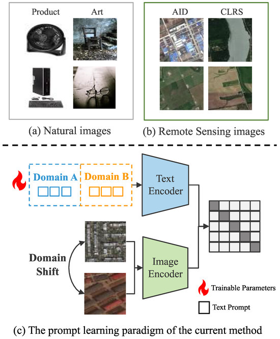
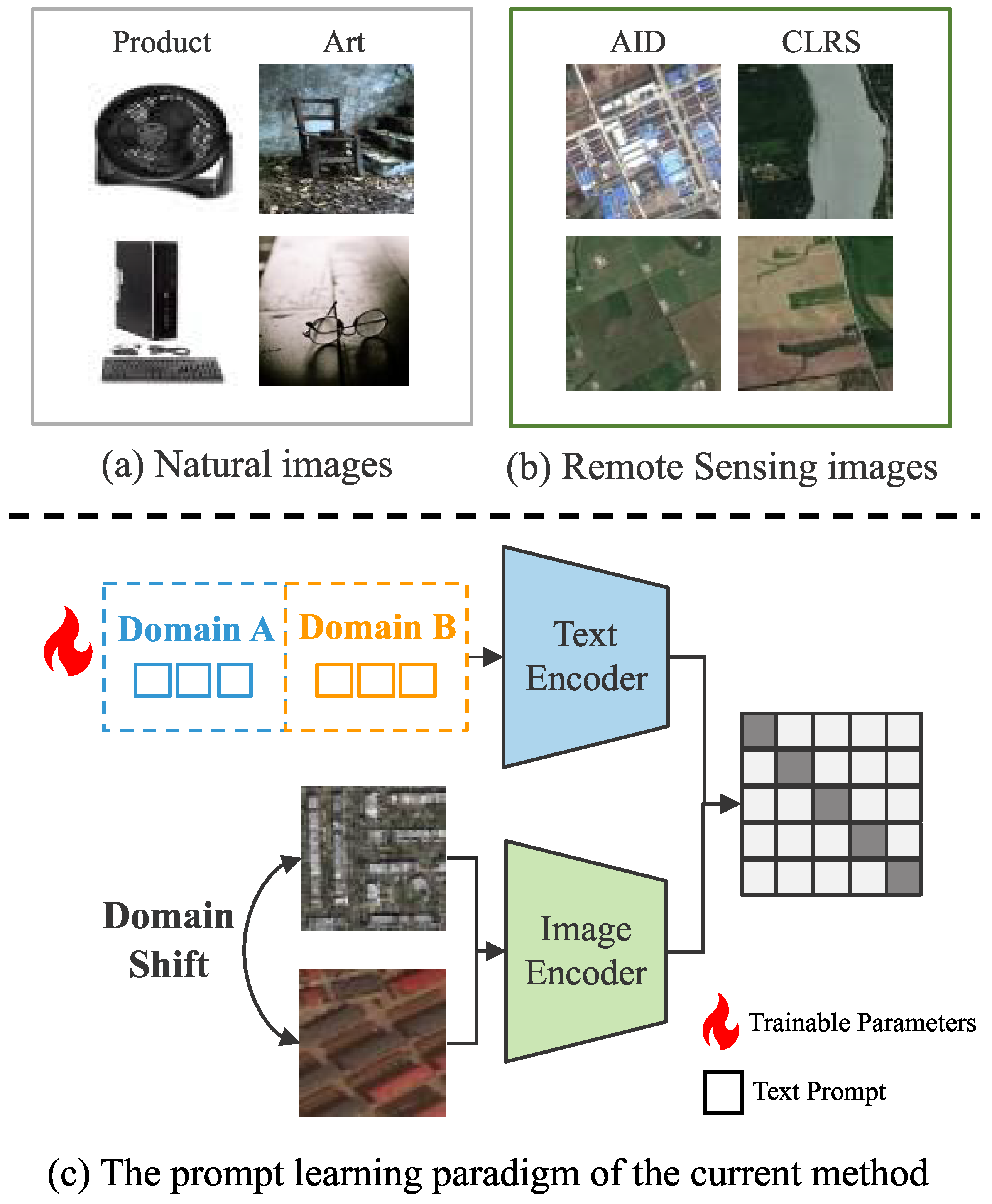
In recent years, large-scale pre-trained Visual-Language Models (VLMs), such as CLIP [24] and ALIGN [25], have demonstrated exceptional performance across a wide range of downstream tasks. Specifically, the CLIP model has been pre-trained on large-scale image-text pairs for contrastive learning, enabling it to acquire extensive visual-language features and the ability to perform effective zero-shot classification. To improve the model’s classification performance on data with different distributions, Coop [26] enhances the model’s classification performance in different domains by using context prompts as learnable parameters and prompt-based fine-tuning with a small amount of available labeled data. DAPrompt [27] decouples domain features from category features by learning both domain-specific and domain-agnostic prompts. However, this approach of learning source- and target-domain-specific prompts for prediction performs poorly on remote sensing image datasets, leading to weak cross-domain transfer. As shown in Figure 1, Existing methods perform well on natural image cross-domain datasets by learning domain-specific prompts, as there is a high consistency in style and content within the same domain, and domain-specific information is clear, making it easier for the model to learn effective domain-specific prompts. However, in cross-domain remote sensing image datasets, variations in land cover elements within the same domain are highly diverse, making it difficult for the model to generalize domain-specific information solely from text features. This, in turn, makes the learning of domain-specific prompts more challenging. Moreover, current methods fail to reduce the domain shift between the source and target domains and do not fully utilize the rich knowledge from the source domain.

Figure 1. Panels (a,b) illustrate the differences between natural images and remote sensing images. In natural images, visual characteristics are relatively uniform, such as in the Art and Product domains. In contrast, in remote sensing images, visual characteristics are highly diverse. Panel (c) presents the learning paradigm of current domain-specific learning methods.

To address the above issues, we propose a new cross-domain scene classification method called DIPVR, which leverages CLIP to learn Domain-Invariant Prompts and Visual Representations to reduce the distribution discrepancy between the source and target domains, and improve the model’s cross-domain transfer performance. Specifically, the main idea is to learn domain-invariant prompts and domain-invariant visual features to extract common features across domains by matching visual and semantic features. We aim to learn domain-invariant prompts rather than domain-specific ones and introduce prior knowledge to enhance semantic feature generation. To learn visually invariant features, we propose a visual-invariant learning method that can be well integrated with the structure of VLMs by attentively and adaptively capturing common features across the source and target domains. Specifically, while conventional methods often rely on domain-specific prompts that are easily compromised by the inherent land-cover heterogeneity within remote sensing domains, our approach advocates a conceptual shift toward domain-invariant prompts coupled with visual invariance. This dual-path alignment enables the model to bypass domain-specific noise and capture robust, domain-agnostic semantic and feature representations across diverse geographic distributions. The main contributions of this paper are as follows:

• We introduce DIPVR, an advanced cross-domain scene classification approach that leverages domain-invariant prompts and visual representations to improve the model’s performance in the target domain by extracting the common features of the two modalities, with domain alignment achieved through feature matching.
• We propose learning domain-invariant prompts and utilizing prior knowledge to guide the process, enhancing cross-domain scene classification performance through prompt learning with the CLIP model.
• We propose a Visual Invariant Learning module to learn domain-invariant visual representations, which leverages attention mechanisms to extract common features from the representative features of both the source and target domains.

2. Related Work

2.1. Cross-Scene Interpretation

In recent years, significant progress has been made in cross-domain interpretation techniques for remote sensing images, which have been applied in many downstream tasks. These techniques aim to address differences in data distribution across scenes or sensors, which often lead to performance degradation when models trained on one dataset are applied to another.

To tackle this challenge, various methods have been proposed. APDM [28] effectively resolves the issues of high background complexity and low category consistency in remote sensing images by utilizing pairwise cosine discrepancy and nuclear norm optimization to suppress negative semantic features and implicitly align cross-scene distributions. ClA-UDA [29] significantly enhances the performance of cross-domain semantic segmentation in high-resolution remote sensing images through category-level assignment and image style transformation. CACL [30] improves cross-scene hyperspectral image classification performance by employing domain-level and class-level distribution alignment, along with a customized learning strategy targeting the target samples to transfer the supervised information from the source domain. MDA-NET [31] combines multi-source data (such as hyperspectral images and LiDAR data) to significantly enhance cross-scene classification performance through multi-level domain adaptation and modality collaboration.

2.2. Domain Adaptation

To address the challenges of domain distribution discrepancy and the difficulty of obtaining labeled data, domain adaptation transfers knowledge from the source domain, thereby enhancing the generalization ability of models in the target domain and reducing reliance on large amounts of labeled target data. With the rise of deep learning, deep learning-based domain adaptation methods have demonstrated superior performance and become the mainstream research direction. These methods are primarily categorized into moment-matching-based methods and adversarial training-based methods.

In the moment-matching-based methods, DAN [15] reduces the distribution discrepancy between source and target domains by matching mean embeddings using Multi-Kernel Maximum Mean Discrepancy (MK-MMD). DSAN [18] aligns the distributions of relevant subdomains using Local Maximum Mean Discrepancy (LMMD). This approach captures fine-grained information for each category without adversarial training, making it easy to implement and fast to converge.

Adversarial training-based methods utilize feature extractors and classifiers for adversarial training to perform implicit feature alignment. MCD [19] maximizes the discrepancy between two classifiers’ outputs to identify target samples far from the source support, aligning distributions while considering task-specific decision boundaries. SCDA [32] uses pair-wise adversarial alignment of prediction distributions to suppress irrelevant semantic information and accentuate principal features, improving adaptation performance. DALN [22] reuses the task-specific classifier as a discriminator, leveraging a Nuclear-norm Wasserstein discrepancy (NWD) to guide feature alignment without additional weight clipping or gradient penalties. However, previous approaches only migrate across domains from the visual backbone, missing the semantic level of understanding to adapt to some complex tasks.

2.3. Vision–Language Models and Prompt Learning

VLMs exhibit strong multimodal understanding due to large-scale pre-training, and especially CLIP demonstrates better performance compared to past vision-based methods in many downstream tasks [32,33,34,35,36].

To enable VLMs to efficiently adapt to downstream tasks, inspired by the NLP field [37], Prompt Learning has been introduced to visual tasks. In prompt learning, soft prompts are automatically learned to guide the model’s focus on key information. This approach reduces the number of fine-tuned parameters, improving task adaptability and enhancing data efficiency and generalization performance. Coop [26] introduces learnable context prompts for efficiently adapting Vision–language Models (VLMs) to downstream tasks with few-shot labeled data, while CoCoOp [38] further improves generalization to unseen classes by leveraging conditional prompt learning. MaPLe [39] introduces multi-modal prompt learning for vision–Language models by jointly tuning both vision and language branches, ensuring better alignment and generalization across tasks, outperforming prior uni-modal prompting methods.

In order to fully utilize the knowledge of CLIP and source domains, researchers try to use CLIP for domain adaptation. DAPrompt [27] introduces a novel prompt-learning paradigm for unsupervised domain adaptation, leveraging domain-specific prompts rather than conventional domain alignment to preserve semantic information, achieving state-of-the-art performance across multiple benchmarks. However, there are two major limitations when applying such methods to remote sensing scenarios. First, DAPrompt learns domain-specific prompts; in remote sensing tasks characterized by high intra-class diversity and complex land cover changes, these specific prompts may overfit to local domain noise rather than capturing the core semantic categories. Second, these methods primarily focus on the language branch and do not explicitly reduce the inherent domain shift in the visual feature space. In contrast, our proposed DIPVR distinguishes itself by learning domain-invariant prompts informed by remote-sensing-specific prior knowledge. By enforcing invariance in both the prompt space and the visual representation space, DIPVR not only preserves the zero-shot generalization capability of CLIP but also actively minimizes the distribution discrepancy between source and target domains, making it more robust for specialized cross-domain scene classification.

3. Method

3.1. Preliminaries

Let the source domain $D_s={\{{\mathit{x}}_i^s,y_i^s\}}_{i=1}^{N_s}$, which contains $N_s$ labeled samples. Meanwhile, the target domain $D_t={\left\{{\mathit{x}}_i^t\right\}}_{i=1}^{N_t}$ consists of $N_t$ unlabeled samples. These two domains have different feature distributions but share the same set of labels. The goal of cross-domain scene classification is to learn a model $f:X\to Y$ on top of $D_s$ and $D_t$ to give good performance on the target domain.

3.2. Overview

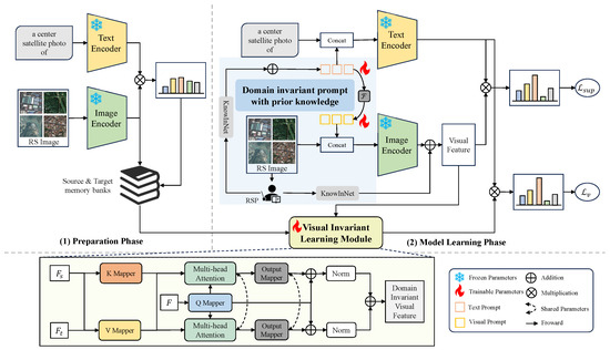
The proposed method includes a preparation phase and a model learning phase, as shown in Figure 2. To provide a systematic understanding of the framework, we describe the pipeline through two main phases: the preparation phase and the model learning phase, emphasizing the roles and interactions of key components.

Figure 2. The overall model consists of two processes: the preparation phase and the model training phase. The model training phase is the key component. In the preparation phase, the original CLIP is used to construct memory banks for both the source and target domains, laying the groundwork for subsequent visual-invariant learning. During model training, the language branch learns domain-invariant prompts and leverages prior knowledge to guide enhancement. In the visual branch, a Visual-Invariant Learning module is employed to learn shared visual features between the source and target domains. The features in the memory banks for the source and target domains are denoted as $F_s$ and $F_t$, respectively, while the features extracted by our image encoder are referred to as F. $\mathcal{F}$ is the transformation network for the two-modal prompts. Domain alignment is achieved by matching domain-invariant context and visual features. Two loss functions are designed: ${\mathcal{L}}_{sup}$ is the supervised learning loss, and ${\mathcal{L}}_v$ is the visual-invariant loss.

• Preparation Phase: This phase focuses on establishing a stable starting point for domain alignment. Specifically, we utilize the CLIP visual encoder to initialize two memory banks ($F_s$ and $F_t$), which serve as repositories for source and target feature prototypes. These memory banks are crucial as they provide global structural information and stable contrastive samples for the subsequent learning process.
• Model Learning Phase: In this phase, we perform dual-path invariant learning to bridge the domain gap:

  –

  In the language path, we implement domain-invariant prompt learning guided by remote sensing-specific prior knowledge, ensuring the semantic descriptions remain consistent across domains.

  –

  In the vision path, we conduct visual invariant learning to minimize the distribution discrepancy between source and target features.

• Interaction: The memory banks act as a bridge between these two paths, providing updated feature anchors to guide both prompt calibration and visual feature alignment. By integrating these components, the model iteratively refines its ability to capture domain-agnostic representations.

3.3. Domain-Invariant Prompt with Prior Knowledge

CLIP is a multimodal pre-trained model based on contrastive learning, and its core idea is to train the image encoder $f_v(·)$ and the text encoder $f_t(·)$ on large-scale image-text pairs data, so that semantically related images and texts have higher similarity in the shared feature space. Specifically, given a set of image-text pairs, CLIP is trained to maximize the similarity of correctly matched pairs and minimize that of incorrectly matched pairs.

In the inference phase, CLIP relies on a zero-shot learning mechanism for classification. Specifically, given an input image $\mathit{x}$, CLIP computes its visual feature $f_v\left(\mathit{x}\right)$ and matches its similarity with a text embedding ${\left\{f_t\left({\mathit{t}}_k\right)\right\}}_{k=1}^K$ of K categories. The final category prediction is obtained by softmax normalization:

$$P(\mathit{y}=k\mid \mathit{x})={\displaystyle \frac{exp\left(\mathrm{sim}\left(f_v\left(\mathit{x}\right),f_t\left({\mathit{t}}_k\right)\right)/T\right)}{{\sum }_{j=1}^{K}exp\left(\mathrm{sim}\left(f_v\left(\mathit{x}\right),f_t\left({\mathit{t}}_j\right)\right)/T\right)}}$$

(1)

where T is the temperature parameter, $\mathrm{sim}(·,·)$ denotes the cosine similarity, and ${\mathit{t}}_k$ is the context prompt corresponding to category k, e.g., “a photo of a [CLS]”.

To enhance adaptability, CoOp [26] replaces these manual prompts with a set of M learnable context vectors $P_t=\{{\mathbf{v}}_1,{\mathbf{v}}_2,\dots ,{\mathbf{v}}_M\}$, each sharing the same dimensionality as the word embeddings. For category k, the prompt ${\mathbf{t}}_k$ is formally defined as the concatenation of these learnable tokens and the category’s word embedding ${\mathbf{c}}_k$:

$${\mathbf{t}}_k=\{{\mathbf{v}}_1,{\mathbf{v}}_2,\dots ,{\mathbf{v}}_M,{\mathbf{c}}_k\}.$$

(2)

Building on this, MaPLe [39] introduces multimodal prompt learning by jointly optimizing context prompts $P_t$ and visual prompts $P_v$. Specifically, MaPLe employs a coupling function $\mathcal{F}$ to derive visual prompts from the language branch ($P_v=\mathcal{F}\left(P_t\right)$), ensuring synergistic alignment across modalities.

Formally, let $\mathit{x}$ denote an input image and ${\mathbf{c}}_k$ represent the word embedding of the k-th category label. In the original CLIP model, these are encoded as $f_v\left(\mathit{x}\right)$ and $f_t\left({\mathbf{c}}_k\right)$, respectively. In our multi-modal prompt learning framework, we introduce learnable prompts into both modalities, resulting in the following prompt-tuned representations:

$$f_v(\mathit{x},P_v),f_t({\mathbf{c}}_k,P_t),$$

where $P_v$ and $P_t$ act as modality-specific adaptations that refine the feature extraction process. By jointly optimizing $P_v$ and $P_t$ across the hierarchy of the Vision–Language Model (VLM), our approach achieves superior alignment between visual and semantic modalities, thereby enhancing the model’s generalization capability for remote sensing scene classification.

Since CLIP learns general visual features, while remote sensing images possess specific characteristics, it is necessary to tailor prompts to learn their unique features. The remote sensing pre-trained model(RSP) utilizes large-scale remote sensing data for pre-training, and we believe that it learns to have rich knowledge of remote sensing images. Therefore, we use RSP as an a priori knowledge guide to enhance domain-invariant learning and provide reliable knowledge for the model in terms of both text and image features. In this paper, Wang’s pre-trained model [40] is used as the RSP. For a batch of remote sensing images with a batch size of B, we denote the domain knowledge features of the i-th output after the RSP as ${\mathit{e}}_i$, where $i\in \{1,2,\dots ,B\}$.

For the language branch, features are averaged along the batch dimension to obtain $\overline{\mathit{e}}$, which serves as generic features for remote sensing. The features extracted by the ViT model are high-level semantic representations that are strongly associated with the specific task [41]. Similarly, the features output from RSP are also high-level, with the mean value retaining the commonality of remote sensing data. This allows the extraction of abstract-domain semantic patterns, capturing global semantic information closer to a linguistic level of understanding. To make this more intuitive, the prior knowledge injected into the prompts can be understood as capturing common characteristics of remote sensing imagery, such as typical land-cover elements (e.g., farmland, forest, residential areas), imaging geometry (e.g., top-down or centered satellite view), and acquisition styles (e.g., multi-scale resolution and geographic diversity). Unlike manually designed text templates, these patterns are implicitly encoded as high-level semantic features learned by the remote sensing pre-trained model and projected into the prompt space, enabling the model to better align category semantics with remote sensing-specific characteristics.

We implement KnowInNet ($f_N$) as a three-layer bottleneck MLP with ReLU activation to project RSP features into the prompt space. This architecture enables the efficient integration of remote sensing prior knowledge while filtering redundant information to enhance domain-invariant learning. Then, we add it to $P_t$ to obtain the prior context feature, denoted as ${\widehat{P}}_t$:

$${\widehat{P}}_t=P_t+f_N\left(\overline{\mathit{e}}\right)$$

(3)

This makes the context prompts come with prior knowledge from the beginning and does not need to completely rely on the gradient update to adjust the prompts. Moreover, by adding prior knowledge before the category embedding, the CLIP text encoder will receive remote-sensing-related information first when processing the categories, thereby directing the text encoder’s attention toward generating category representations that better match remote-sensing relevance.

In order to further enhance alignment between visual features and content features, we integrate the features output by the RSP with those produced by the visual encoder, thereby enabling the visual features to incorporate prior knowledge. We use the same transformation network as the language branch to add directly to $f_v({\mathit{x}}_i,P_v)$:

$${\widehat{f}}_v({\mathit{x}}_i,P_v)=f_v({\mathit{x}}_i,P_v)+f_N\left({\mathit{e}}_i\right)$$

(4)

Finally, after being guided by prior knowledge, the probability of class k given an input image $\mathit{x}$ is then computed using a contrastive objective:

$$\widehat{P}(\mathit{y}=k\mid \mathit{x})={\displaystyle \frac{exp\left(\mathrm{sim}\left({\widehat{f}}_v(\mathit{x},P_v),f_t({\mathit{c}}_k,{\widehat{P}}_t)\right)/T\right)}{{\sum }_{k=1}^{K}exp\left(\mathrm{sim}\left({\widehat{f}}_v(\mathit{x},P_v),f_t({\mathit{c}}_k,{\widehat{P}}_t)\right)/T\right)}}$$

(5)

For the source domain, the supervised loss for the source domain is defined as

$${\mathcal{L}}_{sup}^s=-\sum _{i=1}^{N_s}log\widehat{P}\left(y_i^s\mid {\mathit{x}}_i^s\right).$$

(6)

For the target domain, we assign pseudo-labels to the unlabeled target domain. Based on these generated pseudo-labels, the supervised loss for the target domain is defined as

$${\mathcal{L}}_{sup}^t=-\sum _{i=1}^{N_t}log\widehat{P}\left({\widehat{y}}_i^t\mid {\mathit{x}}_i^t\right),$$

(7)

where ${\widehat{y}}_i^t$ is a pseudo-label generated based on the threshold $\tau$ (satisfying $\underset{k}{max}P(k\mid {\mathit{x}}_i^t)\ge \tau$).

3.4. Visual Invariant Learning Module

Learning domain-invariant prompts while improving the model’s downstream task performance does not reduce differences in the feature distributions of source and target domain data. This results in extracted visual features that have domain bias and do not match well with context features, thus limiting the performance of the model. Domain adaptation is essentially an attempt to extract features that are common to both the source and target domains, so this paper extends this idea by proposing a Visual-Invariant Learning module, which combines well with the prompt learning method to further enhance the performance of the model.

Before inputting features into this module, it is necessary to obtain the memory banks for the source and target domains, which hold the centroid features for each category in each domain. For the target domain, we leverage the powerful zero-shot prediction capability of the CLIP model and use the category corresponding to the maximum probability predicted by the output of the original CLIP model as the pseudo-label for the target domain data. For each category in the target domain, the samples corresponding to the top-N largest predicted probabilities are selected, and the features of the selected samples for each category are averaged and saved to the memory banks. For the source domain, we select the samples with the top-N highest prediction probabilities for each category among the correctly predicted samples, and store the features of each category in the memory bank after averaging. Here, we notate the features in the memory banks for the source and target domains as $F_s$ and $F_t$.

Previous cross-domain scene classification methods are designed with specific adaptation losses based on unimodal visual models, which do not integrate well with VLMs. In this paper, we propose an attention-based alignment method that dynamically weights input features based on their importance to further improve cross-domain migration performance. It does not require additional design of the loss function and can be optimized using only the cross-entropy loss.

Here, the features extracted by our image encoder are called F. Then we take F as the query, $F_s$ and $F_t$ form the key and the value. Firstly, we first perform the feature transformation on F, $F_s$, and $F_t$, respectively. We employ three separate mappings for the query, key, and value, named Q Mapper ($f_M^Q$), K Mapper ($f_M^K$), and V Mapper ($f_M^V$). The transformed features are obtained, which can be formulated as

$$\begin{array}{cccccc}\hfill Q& =f_M^Q\left(F\right),\hfill & \hfill K_t& =f_M^K\left(F_t\right),\hfill & \hfill K_{\mathrm{s}}& =f_M^K\left(F_s\right),\hfill \\ \hfill V_t& =f_M^V\left(F_t\right),\hfill & \hfill V_s& =f_M^V\left(F_s\right).\hfill & \hfill & \hfill \end{array}$$

We use a multi-head attention mechanism to extract domain-invariant visual features, which can be well embedded into VLMs. Dual attention branches are computed by weighting visual features with representative features from the source and target domains, respectively, which can mitigate inter-domain distributional differences by capturing diverse feature associations between the source and target domains, and the model can more robustly identify shared features across domains. Specifically, the attention of each head for the source domain and the target domain, named as $A_s^i$, $A_t^i$, is calculated as follows:

$$A_d^i=\mathrm{softmax}\left({\displaystyle \frac{Q_d^i{\left(K_d^i\right)}^T}{\beta }}\right)V_d^i,d\in \{s,t\}$$

(8)

where $\beta$ is the scale parameter. Then the final overall domain-aware features are obtained through the concatenation operation:

$$A_d=\mathrm{Concat}(A_d^1,A_d^2,\dots ,A_d^h),d\in \{s,t\}$$

(9)

where d stands for a domain, and h represents the number of attention heads, which is set to 8 here. The domain-aware features are then transformed by the Output Mapper, denoted as $f_M^O$. To improve the discriminative nature of the features, for each branch, we separately overlay the original features onto the domain-aware features and proceed to feature normalization, which can be formulated as:

$${\widehat{F}}_d={\displaystyle \frac{F_d+f_M^O\left(A_d\right)}{\parallel F_d+f_M^O\left(A_d\right){\parallel }_2}},d\in \{s,t\}.$$

(10)

The domain-invariant visual features, denoted as $\widehat{F}$, are obtained through mean aggregation as follows:

$$\widehat{F}={\displaystyle \frac{{\widehat{F}}_s+{\widehat{F}}_t}{2}}.$$

(11)

This feature effectively captures the shared characteristics of both the source and target domains, while preserving the discriminability of the categories.

Finally, the probability of class k given an input image $\mathit{x}$ is then computed as follows:

$${\widehat{P}}_v(\mathit{y}=k\mid \mathit{x})=\left({\displaystyle \frac{exp\left(\mathrm{sim}\left(\widehat{F},f_t({\mathit{c}}_k,{\widehat{P}}_t)\right)/T\right)}{{\sum }_{k=1}^{K}exp\left(\mathrm{sim}\left(\widehat{F},f_t({\mathit{c}}_k,{\widehat{P}}_t)\right)/T\right)}}\right).$$

(12)

The domain-invariant features and context features are matched to minimize the cross-entropy loss for both source and target domains, which is calculated as follows:

$${\mathcal{L}}_v^s=-\sum _{i=1}^{N_s}log\left({\widehat{P}}_v\left(y_i^s\mid {\mathit{x}}_i^s\right)\right),$$

(13)

$${\mathcal{L}}_v^t=-\sum _{i=1}^{N_t}log\left({\widehat{P}}_v\left({\widehat{y}}_i^t\mid {\mathit{x}}_i^t\right)\right).$$

(14)

3.5. Overall Training Objective

We use ${\mathcal{L}}_{sup}$ to denote the total supervised loss across the two domains and ${\mathcal{L}}_v$ to denote the total visual-invariant learning loss across the two domains. The final loss function consists of the supervised loss and visual invariant learning loss. The final overall loss is given by (6) to (14):

$${\mathcal{L}}_{total}={\mathcal{L}}_{sup}+{\mathcal{L}}_v.$$

(15)

3.6. Training Procedure

To improve the clarity of the proposed method, we summarize the overall training procedure of DIPVR in a step-by-step manner as follows:

(1) Representative sample selection: For each mini-batch, source samples are used directly with their ground-truth labels. For target samples, pseudo-labels are generated based on prediction confidence, and only high-confidence samples are selected according to a threshold and top-N strategy.

(2) Domain-invariant prompt learning: The learnable prompts are initialized and updated through backpropagation, guided by prior knowledge extracted from the remote sensing pre-trained model. These prompts aim to align visual features with category semantics across domains.

(3) Visual invariant learning: The visual invariant branch operates on features extracted by the frozen encoder, enforcing consistency between source and target representations to reduce domain discrepancies.

(4) Joint optimization: The model is trained by jointly optimizing the supervised loss on the source domain, the pseudo-label-based loss on the target domain, and the visual alignment loss, enabling collaborative learning of domain-invariant representations.

4. Experiments

In this chapter, we introduce the experimental datasets and the experimental setup. To validate the effectiveness of the proposed method, we compare its performance with several baseline methods. Furthermore, we further demonstrate the superiority of our method from multiple perspectives.

4.1. Datasets

We use existing publicly available remote sensing scene classification datasets to construct cross-domain scene classification tasks. The details of each dataset are as follows:

AID [42]: The AID dataset is a large-scale benchmark dataset for aerial scene classification, consisting of 10,000 high-resolution images covering 30 scene categories. The images, collected from Google Earth, originate from diverse geographic regions around the world, ensuring high intra-class diversity and low inter-class dissimilarity. Each image is 600 × 600 pixels in size, with varying spatial resolutions ranging from 8 to 0.5 m per pixel.

CLRS [43]: The CLRS dataset contains 15,000 remote sensing images covering 25 scene categories, each containing 600 images of 256 × 256 pixels. The resolution of the images ranges from 0.26 to 8.85 m and covers more than 100 countries and regions around the world.

MLRSN [44]: The MLRSN dataset contains 109,161 high-resolution optical satellite or aerial images covering 46 scene categories, with each image containing one or more of the predefined labels from a set of at least 60. Image resolutions range from approximately 10 m to 0.1 m, with each image having a fixed size of 256 × 256 pixels.

RSSCN7 [45]: The RSSCN7 dataset consists of 2800 high-resolution remote sensing scene images, covering seven typical scene categories. Each category contains 400 images, which are collected from Google Earth and sampled at four different scales, with 100 images per scale. Each image has a fixed size of 400 × 400 pixels.

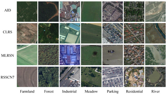
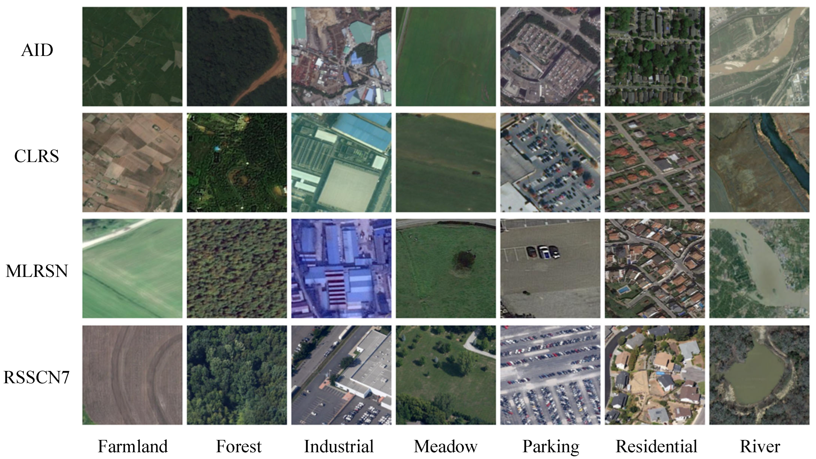
In the experiments, images from seven shared scene categories were selected for cross-domain scene classification: Farmland, Forest, Industrial, Meadow, Parking, Residential, and River, as shown in Figure 3. In image preprocessing, we resize the images to 256 × 256 and then randomly crop them to 224 × 224. Given the phenomenon that various types of residential areas always exist in these datasets, we choose “Residential” or “Dense Residential” as the residential category. The detailed information of the selected samples is shown in Table 1. We consider these four datasets as four different domains: AID (A), CLRS (C), MLRSN (M), and RSSCN7 (R). For cross-domain scene classification, we only consider single-source to single-target domain adaptation, designing 12 cross-domain scene classification tasks.

Figure 3. Image display of each category from the four datasets.

Table 1. The specific quantities of the four datasets.

Class	AID	CLRS	MLRSN	RSSCN7
Farmland	370	600	501	400
Forest	250	600	501	400
Industrial	390	600	422	400
Meadow	280	600	501	400
Parking	390	600	501	400
Residential	410	600	1058	400
River	410	600	500	400
Total	2500	4200	3984	2800

4.2. Experimental Setup

4.2.1. Compared Methods

We compare our proposed method with the following state-of-the-art methods: (1) Source-only: This method is trained using only source domain data and tested directly in the target domain, representing no adaptation. (2) Unimodal vision-based methods: DANN [20], MCD [19], MDD [46], BSP [47], BNM [48], DALN [22], APDM [28]. (3) VLM-based methods: DAPrompt [27]. Additionally, we used the original CLIP for comparison as a baseline for VLM-based methods to evaluate performance differences. We use the classification accuracy of all cross-domain scene classification tasks as an evaluation metric.

4.2.2. Implementation Details

In this work, we focus on the unsupervised domain adaptation (UDA) scenario, where no labeled samples are available in the target domain. This setting reflects common real-world situations in remote sensing, where annotating new datasets is costly and labor-intensive. Our method is designed to operate under this fully unsupervised setting, and does not rely on any labeled data from the target domain. We use labeled data from the source domain and unlabeled data from the target domain for training and testing in the target domain. Our experiments are implemented in the Pytorch 1.8 framework, running on a GeForce RTX 3090. To fairly compare the performance of different DA methods, we control for the same visual encoder across all comparison methods. We use a pre-trained Vit-B/16 [41] as the backbone network to extract visual features. For source-only, unimodal vision-based methods, we fine-tune the backbone network using the training data. For the VLM-based approach, following the prompt-learning setting, we fix the text encoder and visual coder of the model. The comparison methods are all experimented with using the structure and parameters from their original papers. In the model training process, we use SGD [49] as the optimizer and apply a cosine annealing learning rate scheduler, with the initial learning rate set to $1\times {10}^{-5}$. The learning rate of the model is $3\times {10}^{-3}$. When extracting features using the original CLIP model, we refer to the experiments in the Coop paper and design the input prompt for remote sensing images as “a centered satellite photo of.” For the RSP model, we choose the Swin Transformer as the backbone network, fix its parameters, and perform only inference and prediction. The batch size for both the source and target domains is set to 32. For the multimodal prompt learning part, we maintain the same structure and parameters as in Maple to learn both visual and context prompts. We obtain the value of T from the CLIP pre-trained weights, and set $\beta$ to 0.1. The token length is set to 16, and the pseudo-label confidence threshold for the target domain is set to 0.8. Pseudo-labels are assigned only to target samples whose prediction confidence exceeds a predefined threshold $\tau$ (set to 0.8 in our experiments). For samples whose prediction probabilities are all below $\tau$, no pseudo-labels are assigned, and these samples are excluded from pseudo-label-based supervision. Nevertheless, they are still utilized in other training components, such as visual-invariant learning, which does not require pseudo-labels. We set the number of representative samples selected from each domain to 5. The results of the above methods were obtained by averaging over five random experiments.

4.3. Experimental Results

In our experiments, we implement the proposed method based on the ViT-B/16 backbone and compare it with several existing approaches to validate its effectiveness.

The results based on the ViT-B/16 backbone are shown in Table 2. The experimental results show that the proposed method significantly outperforms state-of-the-art methods in cross-domain scene classification, achieving the highest average classification accuracy of 87.66%. Compared to unimodal vision-based methods, our method achieves 2.19% higher average classification accuracy than the best method in this category. This improvement is due to the incorporation of semantic information through multimodal learning, which enhances the model’s ability to distinguish between categories. Additionally, by extracting domain-invariant context and visual features, our method improves the model’s cross-domain transferability. Compared to VLM-based methods, such as DAPrompt, perform poorly due to their reliance on domain-specific prompts, achieving even lower average accuracy than the original CLIP model. Our proposed method, on the other hand, learns domain-unified prompts that effectively capture category-specific context features and extract universal visual features via visual invariance learning, thereby achieving better multimodal feature alignment.

Table 2. Classification accuracies (%) on cross-scene dataset (ViT-B-16). Bold values indicate the best performance for each column.

Method	A-C	A-M	A-R	C-A	C-M	C-R	M-A	M-C	M-R	R-A	R-C	R-M	Average
Source-only	91.69	74.20	73.46	97.02	71.62	73.26	75.34	63.79	60.27	85.64	80.73	54.92	75.16
DANN	96.90	74.61	84.42	98.14	77.01	84.16	79.09	79.75	77.01	95.39	92.77	69.76	84.08
MCD	96.27	72.44	81.97	98.83	73.19	80.31	80.91	77.90	76.14	96.52	89.48	75.19	83.26
MDD	96.31	76.11	83.74	98.93	78.61	83.37	88.67	78.32	76.64	97.49	92.01	75.38	85.47
BSP	96.28	76.04	80.11	98.18	75.16	83.64	74.99	75.56	76.32	96.58	93.65	79.90	83.87
BNM	96.30	69.80	83.07	98.81	69.02	84.19	77.65	78.60	81.74	97.30	91.83	81.00	84.11
DALN	96.14	71.90	82.76	98.82	68.69	84.21	75.70	76.56	79.41	96.70	91.45	81.31	83.64
APDM	94.44	69.92	76.24	98.33	68.84	75.22	81.06	77.35	73.03	96.10	88.76	76.30	81.30
CLIP	76.12	77.11	68.71	86.88	77.11	68.71	86.88	76.12	68.71	86.88	76.12	77.11	77.20
DAPrompt	75.03	73.44	66.69	84.75	73.55	66.88	85.11	74.96	66.71	84.42	75.20	73.83	75.05
Ours	93.23	79.48	83.58	99.30	81.75	81.06	96.52	89.29	78.79	98.38	92.23	78.32	87.66

4.4. Analysis

4.4.1. Ablation Study

We further designed ablation experiments to further validate the role of the key components of the proposed method, and the results are shown in Table 3. Specifically, there are four comparison models: (1) CLIP: This model does not perform prompt learning and only uses raw text prompts. (2) ${\mathcal{L}}_{sup}$: This model has only supervised learning loss. (3) ${\mathcal{L}}_v$: This model has only a visual alignment model loss. (4) w/o Prior Knowledge: This model removes the prior knowledge guidance part, while keeping the other components the same as the proposed method. (5) Ours: The proposed method in this paper. The results from (1) and (2) show that by learning from domain-invariant prompts and guided by prior knowledge, the performance of the model is significantly improved, with an improvement of 8.86% compared to the original model. Specifically, when the domain-invariant prompts are removed, the model tends to rely more heavily on generic or source-biased semantic representations. In this case, we observe that categories with subtle semantic differences but similar visual appearances (e.g., meadow vs. farmland) are more prone to confusion. This is because the prompts no longer effectively encode remote sensing-specific semantic context, leading to weaker alignment between visual features and category semantics. From the comparison between (3) and (5), it can be seen that the supervised learning loss is very important, and the performance of the model without the supervised learning loss decreases by 4.1%. The supervised learning loss can help the model learn more discriminative features across categories, enabling it to better distinguish between them. The comparison between (2) and (5) shows that the visual alignment loss also plays a role, and the performance of the model without the visual alignment loss decreases by 1.6%. The visual alignment loss model better aligns the extracted domain-invariant context features with the visual features, further improving domain adaptation performance. When the visual-invariant learning branch is removed, the model shows greater sensitivity to domain-specific visual variations. In particular, for domain pairs with larger distribution gaps (e.g., differences in resolution, imaging conditions, or geographic regions), the extracted features tend to be biased toward the source domain. This often manifests as overfitting to source-domain textures and appearance patterns, resulting in degraded performance in the target domain. From the comparison of (4) and (5), it can be found that the prior knowledge of remote sensing is also very important to guide the model, and through the enhancement of the context branch and the visual branch, the model is able to extract features that are more compatible with remote sensing characteristics for remote sensing images.

Table 3. Ablation study (%) on the cross-scene dataset (ViT-B/16). Bold values indicate the best performance for each column.

Method	A-C	A-M	A-R	C-A	C-M	C-R	M-A	M-C	M-R	R-A	R-C	R-M	Average
CLIP	76.12	77.11	68.71	86.88	77.11	68.71	86.88	76.12	68.71	86.88	76.12	77.11	77.20
${\mathcal{L}}_{sup}$	92.67	80.46	82.96	99.29	81.48	79.43	90.70	83.98	72.26	98.55	92.00	78.99	86.06
${\mathcal{L}}_v$	84.78	83.99	76.33	91.31	84.44	77.69	88.71	80.59	73.63	92.55	86.17	82.52	83.56
w/o Prior Knowledge	91.33	79.12	82.71	99.22	80.77	80.19	93.20	89.23	82.63	97.94	91.32	79.43	87.26
Proposed Method	93.23	79.48	83.58	99.30	81.75	81.06	96.52	89.29	78.79	98.38	92.23	78.32	87.66

4.4.2. Hyperparameter Analysis

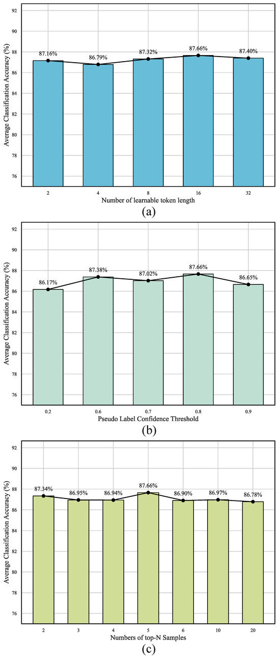
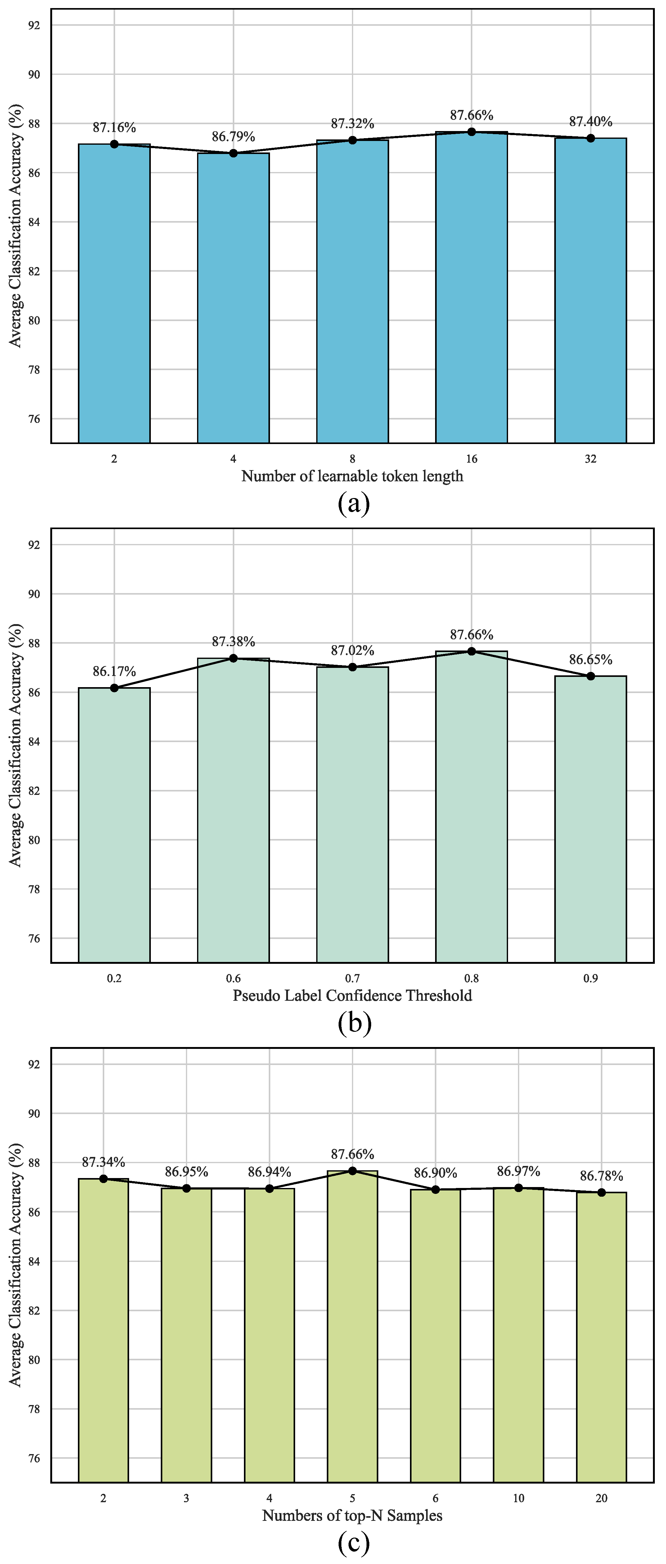
In the proposed method, we analyze the following hyperparameters: the number of learnable tokens, the threshold for pseudo-labels, and the number of top-N samples. As shown in Figure 4a, the model’s performance improves as the length of learnable tokens increases from 4 to 16, indicating that a longer token length enhances the model’s ability to learn richer high-level semantic knowledge and improves feature extraction. However, as the token length continues to increase beyond 16, the model’s performance starts to decline, suggesting that excessively long prompts do not further enhance the model’s performance. Therefore, we set the length of learnable tokens to 16. These results indicate that the performance gain brought by prior knowledge is robust to prompt design choices. Although different token lengths affect prompt capacity, the improvement persists, demonstrating that the model does not rely on fragile prompt formulations but instead benefits from stable and learnable prompt representations.

Figure 4. Hyperparameter analysis. Panel (a) represents the average classification accuracy under different learnable token lengths. Panel (b) represents the average classification accuracy under different pseudo-label thresholds. Panel (c) represents the average classification accuracy under different numbers of top-N samples.

The size of the pseudo-label threshold determines the quality of pseudo-labels for target-domain data and also affects the model’s training performance. Figure 4b shows the classification performance under different thresholds. As shown in the figure, a too-small threshold leads to inaccurate pseudo-labels, causing a decline in model performance. When the pseudo-label threshold increases from 0.6, the model performance fluctuates slightly. The classification performance is best when the threshold is set to 0.8, but performance decreases as the threshold continues to increase. This indicates that the quality of pseudo-labels improves with a higher threshold. However, if the threshold is too high, some noisy labels may be mistakenly considered as high-quality labels, thereby negatively impacting the model’s training effectiveness.

When constructing the memory bank, the number of samples selected from the source and target domains determines the quality of the class features in the memory bank. Figure 4c shows a comparison of classification performance for different numbers of top-N samples selected. From the results, it can be observed that when the number of samples is less than 5, the selected samples are too few, and the class features obtained by averaging these samples cannot adequately represent the characteristics of each class. When the number exceeds 5, even reaching 20, the number of selected samples increases, potentially including some lower-quality samples, which leads to a decrease in the quality of the obtained class features and negatively affects subsequent feature alignment. Therefore, we choose to set the sample size to 5.

Based on the above analysis, we provide several practical recommendations for hyperparameter selection. The number of learnable tokens is a key factor that significantly affects performance, as it controls the capacity of the prompt representation. Empirically, setting the token length within a moderate range (e.g., 8 to 16) achieves a good balance between expressiveness and stability. In contrast, the pseudo-label threshold and the number of top-N representative samples are relatively less sensitive, and stable performance can be obtained within a reasonable range. Therefore, these parameters can be tuned coarsely without requiring exhaustive search. In practice, we adopt default settings that perform consistently well across datasets, simplifying the deployment of the proposed method.

4.4.3. Confusion Matrix

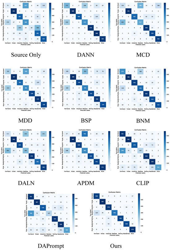
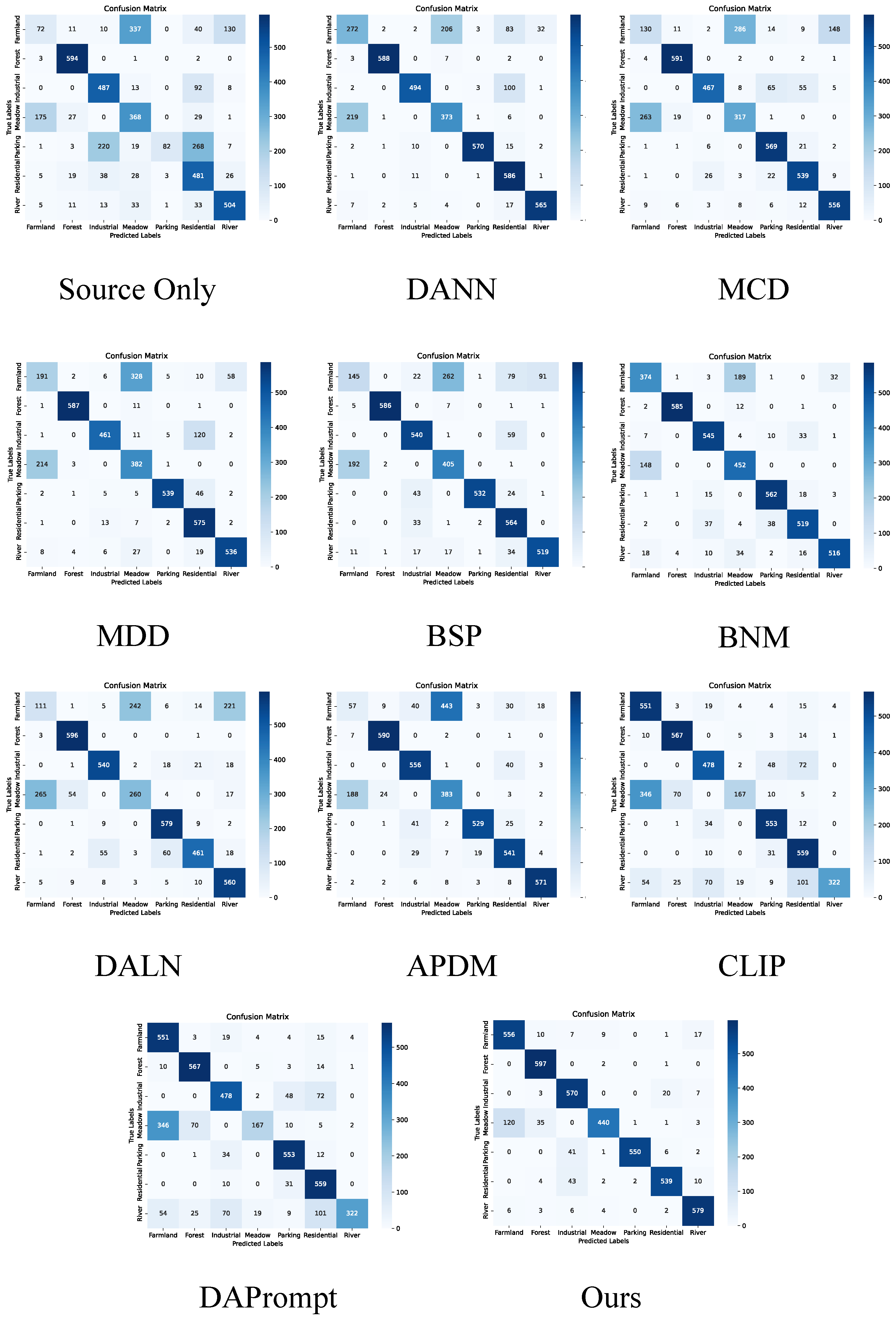
The confusion matrix results of different methods in task M-C are shown in the Figure 5. From the results of the confusion matrix, it can be seen that the source-only model exhibits a significant amount of misclassification. CLIP and DAPrompt show little difference compared to the source-only model. Other domain adaptation methods improve classification performance in the target domain by reducing the discrepancy between the source and target domains, greatly alleviating misclassifications. It is evident that the “Meadow” and “Farmland” classes, due to their similar scenes, are easily misclassified by the model. However, our proposed method, by learning domain-invariant prompts and domain-invariant visual representations and matching both visual and context modalities, not only effectively mitigates confusion between these two classes but also achieves higher classification accuracy across the remaining classes, resulting in better cross-domain classification performance.

Figure 5. Confusion matrix on task M-C across different methods.

4.4.4. t-SNE Visualization

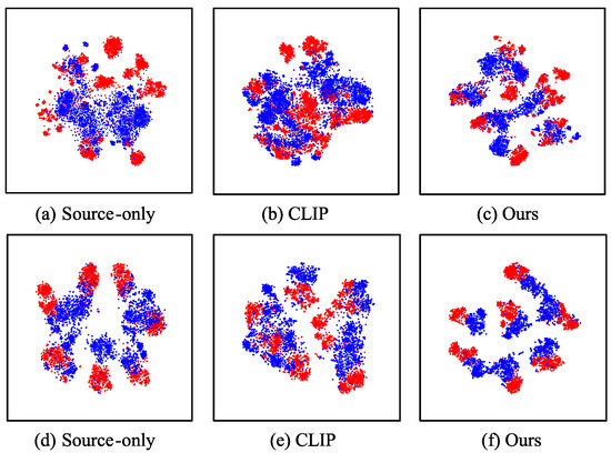
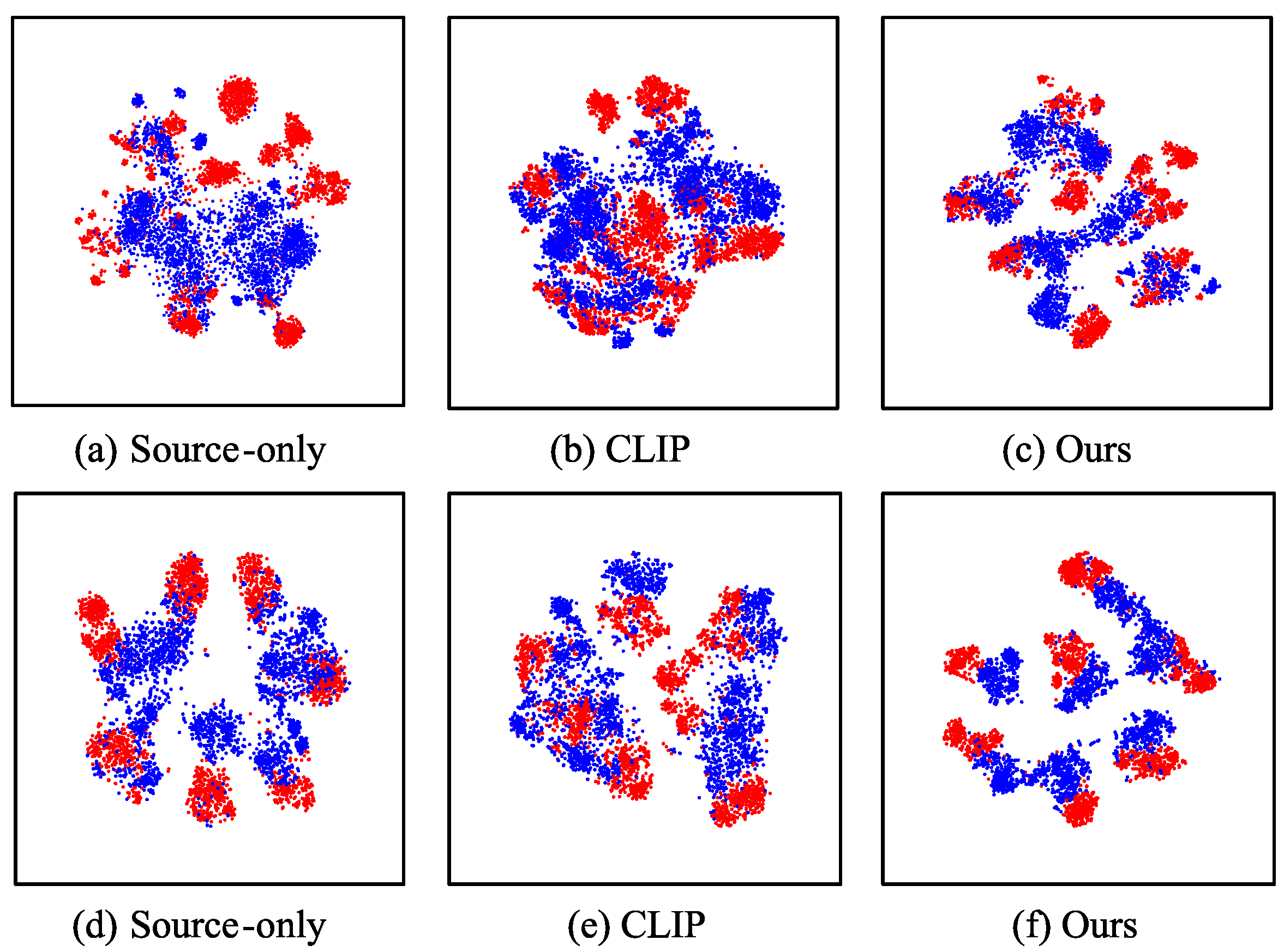
Using ViT-B/16 as the backbone network, we visualized Source-only, Original CLIP, and our proposed method using t-SNE [50] embeddings in different tasks, as shown in Figure 6. The source-only method is trained only on the source domain, and due to the domain shift between the source and target domains, it can be seen that the feature distributions extracted from the two domains differ significantly. The CLIP model, without domain adaptation, also shows a large discrepancy between the features extracted from the source and target domains, with the target-domain features being more dispersed. In contrast, the method proposed in this paper extracts domain-invariant features from both context and visual dimensions. From the visualization results, it is clear that the domain distribution discrepancy is significantly reduced, leading to better class discriminability and achieving improved cross-domain transfer performance.

Figure 6. t-SNE feature visualization, including source-only, original CLIP, and our method. Panels (a–c) represent the task M-C, while panels (d–f) represent the task A-R. Red features represent the source domain, and blue features represent the target domain.

4.4.5. Model Complexity Comparison

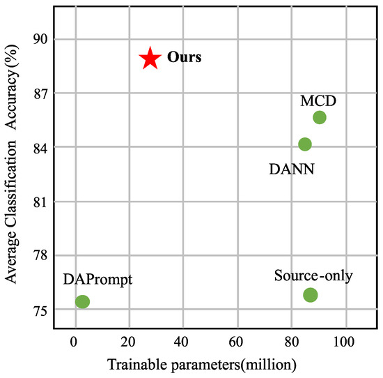
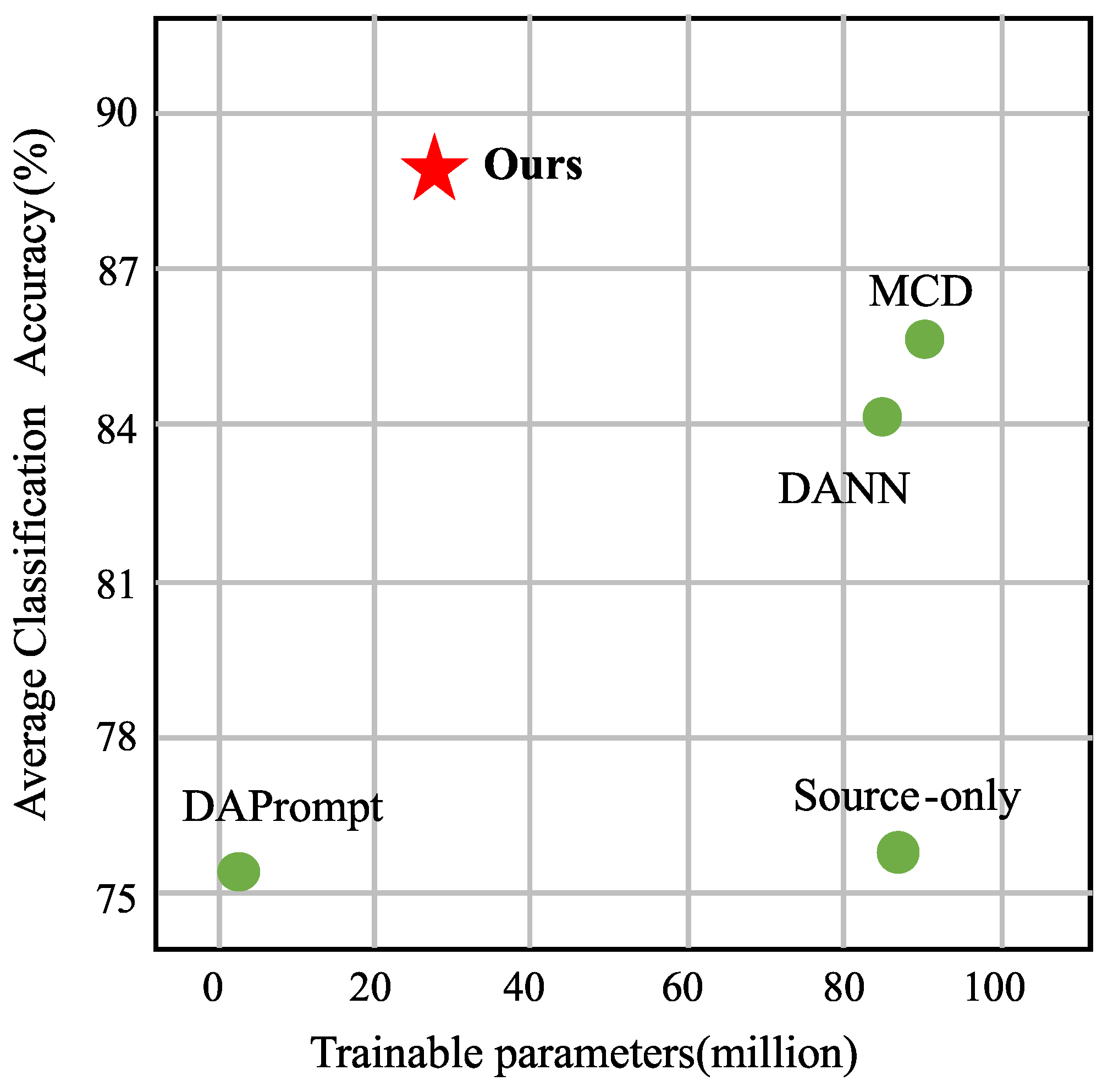
The parameter sizes and corresponding average classification accuracies for different methods are shown in Figure 7. Unimodal vision-based methods typically fine-tune the entire backbone network, resulting in a large number of training parameters but poor performance. Although DAPrompt uses the fewest training parameters, it cannot reduce the discrepancy between the source and target domains because it learns domain-specific prompts. In contrast, our method achieves efficient transfer of VLMs by training only a small number of prompt parameters for the text encoder and a visual-invariant learning module. This enables the achievement of optimal cross-domain classification performance while maintaining a relatively small number of model parameters.

Figure 7. Comparison of the training parameters and corresponding average classification accuracy of different methods.

4.4.6. Efficiency Analysis

To evaluate the practical deployment potential of the proposed method, we conduct a computational efficiency analysis on the AID → MLRSN (A-M) migration task. This task, involving a larger and more diverse target dataset, provides a robust benchmark for testing scalability. The experiments were performed using an NVIDIA GeForce RTX 3090 GPU, and the results are compared with the baseline DAPrompt in Table 4.

Table 4. Comparison of computational efficiency (tested on the A-M task).

Method	Training Time (per Epoch)	Avg Latency (ms/img)	Speed (FPS)
DAPrompt	16 s	1.12	890.26
DIPVR (Ours)	73 s	2.46	407.31

As shown in Table 4, although DIPVR requires more training time per epoch due to the simultaneous optimization of language prompts and visual representations, it maintains a high inference speed of 407.31 FPS. This level of efficiency is well-suited for processing large-scale remote sensing datasets. These results demonstrate that the performance gains achieved by our dual-path alignment strategy do not come at the cost of practical usability, maintaining a favorable balance between accuracy and speed.

5. Conclusions

With the development of VLMs, more and more studies have begun to utilize VLMs to adapt to downstream tasks through prompt-based fine-tuning. Current unsupervised domain adaptation methods based on VLMs are difficult to learn domain-specific prompts for different domains of remote sensing images, and they cannot reduce domain shifts. To address the above issues, we propose a cross-domain scene classification method named DIPVR that learns domain-invariant prompts and visual representations. Specifically, context features common to both source and target domains are extracted by learning domain-invariant prompt learning, and prior knowledge is used to guide the model for feature extraction. In addition, visual features common to the domain are acquired by learning visual-invariant prompts. Finally, domain alignment is performed by matching visual and context features. Experiments on cross-domain scene classification datasets show that the average classification accuracy of our proposed method outperforms all the baseline methods and achieves the best cross-domain migration performance. In the future, we aim to further explore VLMs for domain adaptation, particularly in more realistic and challenging scenarios, such as source-free domain adaptation.

Despite promising results, the current study primarily focuses on cross-dataset transfer across benchmark scene classification datasets, where domain gaps are relatively moderate. In more challenging scenarios, such as transferring across significantly different spatial resolutions, sensor modalities, or large-scale geographic regions, the domain discrepancy may become more pronounced. In such cases, the proposed visual invariant learning module may not be sufficient to fully bridge the gap, as variations in scale, spectral characteristics, and imaging mechanisms can substantially affect feature representations. While domain-invariant prompts can still provide useful high-level semantic guidance, additional mechanisms may be needed to improve robustness. Future work will explore extensions such as multi-scale feature modeling and sensor-aware adaptation strategies to better handle these extreme domain shifts.

Beyond scene classification, the proposed DIPVR framework has the potential to be applied to a broader range of Earth observation tasks. For example, in applications such as high-resolution wetland structure analysis or biomass estimation, both semantic understanding and robustness to domain shifts are crucial. The domain-invariant prompt learning mechanism can help encode task-relevant prior knowledge, such as vegetation structure and spatial patterns, while the visual-invariant learning module can reduce discrepancies caused by different sensors, resolutions, or acquisition conditions. These properties make the proposed framework promising for cross-region and cross-sensor generalization in real-world remote sensing applications.

References

- Lu, C.; Yang, X.; Wang, Z.; Li, Z. Using multi-level fusion of local features for land-use scene classification with high spatial resolution images in urban coastal zones. Int. J. Appl. Earth Obs. Geoinf. 2018, 70, 1–12. [Google Scholar] [CrossRef] [Scilit]
- Fang, F.; Zeng, L.; Li, S.; Zheng, D.; Zhang, J.; Liu, Y.; Wan, B. Spatial context-aware method for urban land use classification using street view images. ISPRS J. Photogramm. Remote Sens. 2022, 192, 1–12. [Google Scholar] [CrossRef] [Scilit]
- Maktab Dar Oghaz, M.; Razaak, M.; Kerdegari, H.; Argyriou, V.; Remagnino, P. Scene and Environment Monitoring Using Aerial Imagery and Deep Learning. In Proceedings of the 2019 15th International Conference on Distributed Computing in Sensor Systems (DCOSS), Santorini Island, Greece, 29–31 May 2019; pp. 362–369. [Google Scholar] [CrossRef] [Scilit]
- Liu, W.; Nie, X.; Zhang, B.; Sun, X. Incremental Learning With Open-Set Recognition for Remote Sensing Image Scene Classification. IEEE Trans. Geosci. Remote Sens. 2022, 60, 1–16. [Google Scholar] [CrossRef] [Scilit]
- Zhao, W.; Bo, Y.; Chen, J.; Tiede, D.; Blaschke, T.; Emery, W.J. Exploring semantic elements for urban scene recognition: Deep integration of high-resolution imagery and OpenStreetMap (OSM). ISPRS J. Photogramm. Remote Sens. 2019, 151, 237–250. [Google Scholar] [CrossRef] [Scilit]
- Wang, Y.; Bashir, S.M.A.; Khan, M.; Ullah, Q.; Wang, R.; Song, Y.; Guo, Z.; Niu, Y. Remote sensing image super-resolution and object detection: Benchmark and state of the art. Expert Syst. Appl. 2022, 197, 116793. [Google Scholar] [CrossRef] [Scilit]
- Piaser, E.; Villa, P. Evaluating capabilities of machine learning algorithms for aquatic vegetation classification in temperate wetlands using multi-temporal Sentinel-2 data. Int. J. Appl. Earth Obs. Geoinf. 2023, 117, 103202. [Google Scholar] [CrossRef] [Scilit]
- Li, Y.; Zhang, Y.; Zhu, Z. Error-Tolerant Deep Learning for Remote Sensing Image Scene Classification. IEEE Trans. Cybern. 2021, 51, 1756–1768. [Google Scholar] [CrossRef]
- Fernando, B.; Habrard, A.; Sebban, M.; Tuytelaars, T. Unsupervised Visual Domain Adaptation Using Subspace Alignment. In Proceedings of the 2013 IEEE International Conference on Computer Vision (ICCV), Los Alamitos, CA, USA, 1–8 December 2013; IEEE: New Yor, NY, USA, 2013; pp. 2960–2967. [Google Scholar] [CrossRef] [Scilit]
- Gong, B.; Shi, Y.; Sha, F.; Grauman, K. Geodesic flow kernel for unsupervised domain adaptation. In Proceedings of the 2012 IEEE Conference on Computer Vision and Pattern Recognition, Providence, RI, USA, 16–21 June 2012; IEEE: New Yor, NY, USA, 2012; pp. 2066–2073. [Google Scholar] [CrossRef] [Scilit]
- Yan, K.; Kou, L.; Zhang, D. Learning Domain-Invariant Subspace Using Domain Features and Independence Maximization. IEEE Trans. Cybern. 2018, 48, 288–299. [Google Scholar] [CrossRef] [Scilit]
- Pan, S.J.; Tsang, I.W.; Kwok, J.T.; Yang, Q. Domain Adaptation via Transfer Component Analysis. IEEE Trans. Neural Netw. 2011, 22, 199–210. [Google Scholar] [CrossRef] [Scilit]
- Wang, J.; Chen, Y.; Hao, S.; Wenjie, F.; Shen, Z. Balanced Distribution Adaptation for Transfer Learning. In Proceedings of the 2017 IEEE International Conference on Data Mining (ICDM), New Orleans, LA, USA, 18–21 November 2017; IEEE: New Yor, NY, USA, 2017; pp. 1129–1134. [Google Scholar] [CrossRef] [Scilit]
- Jing, M.; Zhao, J.; Li, J.; Zhu, L.; Yang, Y.; Shen, H.T. Adaptive Component Embedding for Domain Adaptation. IEEE Trans. Cybern. 2021, 51, 3390–3403. [Google Scholar] [CrossRef] [Scilit] [PubMed]
- Long, M.; Cao, Y.; Wang, J.; Jordan, M. Learning transferable features with deep adaptation networks. arXiv 2015, arXiv:1502.02791. [Google Scholar] [CrossRef] [Scilit]
- Long, M.; Zhu, H.; Wang, J.; Jordan, M.I. Deep transfer learning with joint adaptation networks. arXiv 2017, arXiv:1605.06636. [Google Scholar] [CrossRef] [Scilit]
- Peng, X.; Bai, Q.; Xia, X.; Huang, Z.; Saenko, K.; Wang, B. Moment Matching for Multi-Source Domain Adaptation. In Proceedings of the 2019 IEEE/CVF International Conference on Computer Vision (ICCV), Seoul, Republic of Korea, 27 October–2 November 2019; IEEE Computer Society: Washington, DC, USA, 2019; pp. 1406–1415. [Google Scholar] [CrossRef] [Scilit]
- Zhu, Y.; Zhuang, F.; Wang, J.; Ke, G.; Chen, J.; Bian, J.; Xiong, H.; He, Q. Deep Subdomain Adaptation Network for Image Classification. IEEE Trans. Neural Netw. Learn. Syst. 2021, 32, 1713–1722. [Google Scholar] [CrossRef] [Scilit] [PubMed]
- Saito, K.; Watanabe, K.; Ushiku, Y.; Harada, T. Maximum Classifier Discrepancy for Unsupervised Domain Adaptation. In Proceedings of the 2018 IEEE/CVF Conference on Computer Vision and Pattern Recognition, Salt Lake City, UT, USA, 18–22 June 2018; IEEE Computer Society: Washington, DC, USA, 2018; pp. 3723–3732. [Google Scholar] [CrossRef] [Scilit]
- Ganin, Y.; Lempitsky, V. Unsupervised domain adaptation by backpropagation. arXiv 2015, arXiv:1409.7495. [Google Scholar] [CrossRef] [Scilit]
- Du, Z.; Li, J.; Su, H.; Zhu, L.; Lu, K. Cross-Domain Gradient Discrepancy Minimization for Unsupervised Domain Adaptation. In Proceedings of the 2021 IEEE/CVF Conference on Computer Vision and Pattern Recognition (CVPR), Nashville, TN, USA, 19–25 June 2021; IEEE Computer Society: Washington, DC, USA, 2021; pp. 3936–3945. [Google Scholar] [CrossRef] [Scilit]
- Chen, L.; Chen, H.; Wei, Z.; Jin, X.; Tan, X.; Jin, Y.; Chen, E. Reusing the Task-specific Classifier as a Discriminator: Discriminator-free Adversarial Domain Adaptation. In Proceedings of the 2022 IEEE/CVF Conference on Computer Vision and Pattern Recognition (CVPR), New Orleans, LA, USA, 18–24 June 2022; pp. 7171–7180. [Google Scholar] [CrossRef] [Scilit]
- Goodfellow, I.; Pouget-Abadie, J.; Mirza, M.; Xu, B.; Warde-Farley, D.; Ozair, S.; Courville, A.; Bengio, Y. Generative adversarial nets. arXiv 2014, arXiv:1406.2661. [Google Scholar] [CrossRef] [Scilit]
- Radford, A.; Kim, J.W.; Hallacy, C.; Ramesh, A.; Goh, G.; Agarwal, S.; Sastry, G.; Askell, A.; Mishkin, P.; Clark, J.; et al. Learning transferable visual models from natural language supervision. arXiv 2021, arXiv:2103.00020. [Google Scholar] [CrossRef] [Scilit]
- Li, J.; Selvaraju, R.; Gotmare, A.; Joty, S.; Xiong, C.; Hoi, S.C.H. Align before fuse: Vision and language representation learning with momentum distillation. arXiv 2021, arXiv:2107.07651. [Google Scholar] [CrossRef] [Scilit]
- Zhou, K.; Yang, J.; Loy, C.C.; Liu, Z. Learning to prompt for vision–Language models. Int. J. Comput. Vis. 2022, 130, 2337–2348. [Google Scholar] [CrossRef] [Scilit]
- Ge, C.; Huang, R.; Xie, M.; Lai, Z.; Song, S.; Li, S.; Huang, G. Domain Adaptation via Prompt Learning. IEEE Trans. Neural Netw. Learn. Syst. 2025, 36, 1160–1170. [Google Scholar] [CrossRef] [Scilit] [PubMed]
- Zhu, S.; Wu, C.; Du, B.; Zhang, L. Adversarial pair-wise distribution matching for remote sensing image cross-scene classification. Neural Netw. 2024, 174, 106241. [Google Scholar] [CrossRef] [Scilit] [PubMed]
- Ni, H.; Liu, Q.; Guan, H.; Tang, H.; Chanussot, J. Category-Level Assignment for Cross-Domain Semantic Segmentation in Remote Sensing Images. IEEE Trans. Geosci. Remote Sens. 2023, 61, 1–16. [Google Scholar] [CrossRef] [Scilit]
- Ding, K.; Lu, T.; Fu, W.; Fang, L. Cross-Scene Hyperspectral Image Classification with Consistency-Aware Customized Learning. IEEE Trans. Circuits Syst. Video Technol. 2025, 35, 418–430. [Google Scholar] [CrossRef] [Scilit]
- Zhang, M.; Zhao, X.; Li, W.; Zhang, Y.; Tao, R.; Du, Q. Cross-Scene Joint Classification of Multisource Data with Multilevel Domain Adaption Network. IEEE Trans. Neural Netw. Learn. Syst. 2024, 35, 11514–11526. [Google Scholar] [CrossRef] [Scilit]
- Li, S.; Xie, M.; Lv, F.; Liu, C.H.; Liang, J.; Qin, C.; Li, W. Semantic Concentration for Domain Adaptation. In Proceedings of the 2021 IEEE/CVF International Conference on Computer Vision (ICCV), Montreal, QC, Canada, 11–17 October 2021; IEEE Computer Society: Washington, DC, USA, 2021; pp. 9082–9091. [Google Scholar] [CrossRef] [Scilit]
- Lüddecke, T.; Ecker, A. Image segmentation using text and image prompts. In Proceedings of the IEEE/CVF Conference on Computer Vision and Pattern Recognition, New Orleans, LA, USA, 18–24 June 2022; IEEE Computer Society: Washington, DC, USA, 2022; pp. 7086–7096. [Google Scholar] [CrossRef] [Scilit]
- Jiang, R.; Liu, L.; Chen, C. CLIP-Count: Towards Text-Guided Zero-Shot Object Counting. In Proceedings of the 31st ACM International Conference on Multimedia, New York, NY, USA, 27 October 2023; ACM Digital Library: New York, NY, USA, 2023; pp. 4535–4545. [Google Scholar] [CrossRef] [Scilit]
- Guzhov, A.; Raue, F.; Hees, J.; Dengel, A. Audioclip: Extending Clip to Image, Text and Audio. In Proceedings of the ICASSP 2022-2022 IEEE International Conference on Acoustics, Speech and Signal Processing (ICASSP), Singapore, 23–27 May 2022; IEEE: New York, NY, USA, 2022; pp. 976–980. [Google Scholar] [CrossRef] [Scilit]
- Pan, C.; Yaman, B.; Velipasalar, S.; Ren, L. CLIP-BEVFormer: Enhancing Multi-View Image-Based BEV Detector with Ground Truth Flow. In Proceedings of the 2024 IEEE/CVF Conference on Computer Vision and Pattern Recognition (CVPR), Seattle, WA, USA, 17–21 June 2024; IEEE Computer Society: Washington, DC, USA, 2024; pp. 15216–15225. [Google Scholar] [CrossRef] [Scilit]
- Lester, B.; Al-Rfou, R.; Constant, N. The power of scale for parameter-efficient prompt tuning. arXiv 2021, arXiv:2104.08691. [Google Scholar] [CrossRef] [Scilit]
- Zhou, K.; Yang, J.; Loy, C.C.; Liu, Z. Conditional Prompt Learning for Vision–Language Models. In Proceedings of the 2022 IEEE/CVF Conference on Computer Vision and Pattern Recognition (CVPR), New Orleans, LA, USA, 19–24 June 2022; IEEE Computer Society: Washington, DC, USA, 2022; pp. 16795–16804. [Google Scholar] [CrossRef] [Scilit]
- Khattak, M.U.; Rasheed, H.; Maaz, M.; Khan, S.; Khan, F.S. MaPLe: Multi-modal Prompt Learning. In Proceedings of the 2023 IEEE/CVF Conference on Computer Vision and Pattern Recognition (CVPR), Vancouver, BC, Canada, 18–22 June 2023; IEEE Computer Society: Washington, DC, USA, 2023; pp. 19113–19122. [Google Scholar] [CrossRef] [Scilit]
- Wang, D.; Zhang, J.; Du, B.; Xia, G.S.; Tao, D. An Empirical Study of Remote Sensing Pretraining. IEEE Trans. Geosci. Remote Sens. 2023, 61, 1–20. [Google Scholar] [CrossRef] [Scilit]
- Dosovitskiy, A.; Beyer, L.; Kolesnikov, A.; Weissenborn, D.; Zhai, X.; Unterthiner, T.; Dehghani, M.; Minderer, M.; Heigold, G.; Gelly, S.; et al. An image is worth 16 × 16 words: Transformers for image recognition at scale. arXiv 2021, arXiv:2010.11929. [Google Scholar] [CrossRef] [Scilit]
- Xia, G.S.; Hu, J.; Hu, F.; Shi, B.; Bai, X.; Zhong, Y.; Zhang, L.; Lu, X. AID: A benchmark data set for performance evaluation of aerial scene classification. IEEE Trans. Geosci. Remote Sens. 2017, 55, 3965–3981. [Google Scholar] [CrossRef] [Scilit]
- Li, H.; Jiang, H.; Gu, X.; Peng, J.; Li, W.; Hong, L.; Tao, C. CLRS: Continual Learning Benchmark for Remote Sensing Image Scene Classification. Sensors 2020, 20, 1226. [Google Scholar] [CrossRef] [Scilit] [PubMed]
- Qi, X.; Zhu, P.; Wang, Y.; Zhang, L.; Peng, J.; Wu, M.; Chen, J.; Zhao, X.; Zang, N.; Mathiopoulos, P.T. MLRSNet: A multi-label high spatial resolution remote sensing dataset for semantic scene understanding. ISPRS J. Photogramm. Remote Sens. 2020, 169, 337–350. [Google Scholar] [CrossRef] [Scilit]
- Zou, Q.; Ni, L.; Zhang, T.; Wang, Q. Deep Learning Based Feature Selection for Remote Sensing Scene Classification. IEEE Geosci. Remote Sens. Lett. 2015, 12, 2321–2325. [Google Scholar] [CrossRef] [Scilit]
- Zhang, Y.; Liu, T.; Long, M.; Jordan, M. Bridging theory and algorithm for domain adaptation. arXiv 2019, arXiv:1904.05801. [Google Scholar] [CrossRef] [Scilit]
- Chen, X.; Wang, S.; Long, M.; Wang, J. Transferability vs. discriminability: Batch spectral penalization for adversarial domain adaptation. In Proceedings of the International Conference on Machine Learning, PMLR, Long Beach, CA, USA, 9–15 June 2019; PMLR: Cambridge, MA, USA, 2019; pp. 1081–1090. [Google Scholar]
- Cui, S.; Wang, S.; Zhuo, J.; Li, L.; Huang, Q.; Tian, Q. Towards discriminability and diversity: Batch nuclear-norm maximization under label insufficient situations. In Proceedings of the IEEE/CVF conference on Computer Vision and Pattern Recognition, Seattle, WA, USA, 14–19 June 2020; IEEE Computer Society: Washington, DC, USA, 2020; pp. 3941–3950. [Google Scholar] [CrossRef] [Scilit]
- Song, S.; Chaudhuri, K.; Sarwate, A.D. Stochastic gradient descent with differentially private updates. In Proceedings of the 2013 IEEE Global Conference on Signal and Information Processing, Austin, TX, USA, 3–5 December 2013; IEEE: New York, NY, USA, 2013; pp. 245–248. [Google Scholar] [CrossRef] [Scilit]
- Van der Maaten, L.; Hinton, G. Visualizing data using t-SNE. J. Mach. Learn. Res. 2008, 9, 2579–2605. [Google Scholar]
Disclaimer/Publisher’s Note: The statements, opinions and data contained in all publications are solely those of the individual author(s) and contributor(s) and not of MDPI and/or the editor(s). MDPI and/or the editor(s) disclaim responsibility for any injury to people or property resulting from any ideas, methods, instructions or products referred to in the content. |
© 2026 by the authors. Licensee MDPI, Basel, Switzerland. This article is an open access article distributed under the terms and conditions of the Creative Commons Attribution (CC BY) license.