


Highlights
What are the main findings?
- We propose PAMSTnet, a physics-informed adaptive multiscale spatiotemporal network for long-term global SST prediction that unifies multiscale ocean dynamics learning, cross-variable mode representation, and physics-consistency enforcement with thermodynamic and dynamic constraints.
- PAMSTnet leverages three-dimensional empirical wavelet transform (3DEWT) for interpretable multiscale dynamics learning, multivariate spatiotemporal empirical orthogonal function (MSTEOF) for cross-variable coupled mode representation, and deep ConvLSTM predictive network (DCPN) for coordinated multiscale evolution modeling, and physics-informed consistency learning (PICL) to enforce thermodynamic and dynamic constraints.
What are the implications of the main findings?
- Experiments on global SST predictions demonstrate substantially improved long-term accuracy and robustness to extreme climate variability compared with existing deep learning models, while providing interpretable attribution insights into global SST evolution through physically informed multiscale representations.
- These findings position PAMSTnet as a promising paradigm for intelligent ocean prediction systems that bridge data-driven multiscale representation learning with physics-consistent dynamical modeling, enabling interpretable long-term ocean predictions.
Abstract
Sea surface temperature (SST) serves as a fundamental driver of ocean–atmosphere interactions and global climate variability, exhibiting strong nonstationarity, multiscale dynamics, and cross-variable coupling. However, current deep learning models often fail to capture these complex characteristics, limiting their ability to support accurate and physically consistent long-term SST prediction. To address these issues, we propose PAMSTnet, a unified deep learning framework for physics-informed adaptive multiscale spatiotemporal prediction. PAMSTnet leverages three-dimensional empirical wavelet transform (3DEWT) to learn interpretable multiscale spatiotemporal dynamics from raw observations, and applies multivariate spatiotemporal empirical orthogonal function (MSTEOF) to identify dominant cross-variable coupled modes. These physically meaningful representations are integrated into a deep ConvLSTM predictive network (DCPN) to support coordinated multiscale dynamical learning. Furthermore, PAMSTnet introduces physics-informed consistency learning (PICL) to enforce thermodynamic and dynamic constraints, enhancing physical consistency and interpretability. Extensive experiments demonstrate that PAMSTnet achieves superior performance against state-of-the-art baselines in long-term global SST prediction, reducing RMSE by 8.1% and improving ACC by 2.8% compared with the best-performing baseline, particularly under extreme climate events. Interpretation insights further highlight PAMSTnet’s adaptive representation of variable contributions and regional physical drivers. These findings position PAMSTnet as a promising paradigm for developing intelligent ocean prediction systems with enhanced physical consistency and interpretability.
1. Introduction
Sea surface temperature (SST) serves as a fundamental driver of oceanic dynamical processes, playing a pivotal role in climate regulation, ocean–atmosphere interactions, and the early detection of extreme weather events [1,2,3]. The spatiotemporal variability of SST not only governs the evolution of upper-ocean heat content and wind stress but also exerts far-reaching influences on regional and global climate through teleconnections [4]. Therefore, accurate long-term SST prediction is both theoretically significant and practically important, representing a key objective within the global climate prediction system.
Traditional approaches to SST prediction have primarily relied on dynamical and statistical models. Dynamical models formulate systems of partial differential equations grounded in physical laws to simulate ocean–atmosphere interactions through numerical integration, providing strong theoretical consistency [5,6]. However, their inherent structural complexity, sensitivity to initial and boundary conditions, and accumulation of parameterization errors often lead to systematic biases over mid- to long-range timescales, limiting their adaptability to anomalous perturbations [7]. In contrast, statistical models identify correlations from historical observations and exhibit practical utility in specific regions or under univariate settings. Nevertheless, their limited ability to capture nonlinear, multivariate dynamics restricts their effectiveness in modeling the inherent complexity of real-world climate systems [8,9].
Driven by recent advances in observational coverage and computational capacity, deep learning has emerged as a central methodological paradigm for SST prediction [10,11,12]. Built upon artificial neural networks, these approaches can automatically extract informative features and learn complex nonlinear mappings from raw observations, demonstrating clear advantages over traditional statistical models in pattern recognition and dynamical modeling of climate systems [13,14,15]. Initial efforts in deep learning primarily addressed SST variability from a one-dimensional perspective. Convolutional neural networks (CNNs), for instance, leverage localized receptive fields to capture static spatial patterns and are well-suited for learning regional structures. However, they are limited in capturing the temporal propagation of disturbances and long-range teleconnections [16,17]. Recurrent neural networks (RNNs) and their variants, including long short-term memory (LSTM) and gated recurrent unit (GRU), emphasize long-range temporal dependencies and perform well in representing nonstationary dynamics. Nonetheless, their lack of explicit spatial modeling hinders their ability to capture regional coordination and ocean–atmosphere coupling processes [10,18]. Overall, existing deep learning approaches have yet to fully characterize the coupled spatiotemporal dynamics of SST, thereby limiting their ability to faithfully represent its underlying physical evolution.
To address the limitations of decoupled spatial and temporal modeling, researchers have increasingly developed deep learning models for joint spatiotemporal representation. Convolutional recurrent architectures, exemplified by convolutional LSTM (ConvLSTM), integrate spatial convolutional operations into temporal recurrent process, thereby enhancing the ability to capture short-term dynamical variations and localized propagation patterns [11,19,20,21,22]. Building on this foundation, architectures like predictive RNN (PredRNN) further extend state memory mechanisms, significantly improving the model’s ability to represent nonlinear temporal dependencies [23,24]. Although these approaches have demonstrated promising results in short-term and medium-term prediction tasks, they remain limited by localized perception mechanisms, limiting their capacity to capture the long-range propagation of large-scale perturbations and coordinated spatial evolution. To improve the flexibility of spatial structure modeling, graph neural networks (GNNs) have been introduced to represent spatiotemporal dependencies and complex inter-regional interactions within non-Euclidean geometries [25,26,27]. However, most existing methods rely on static graph topologies, which are inadequate for adapting to time-varying connectivity patterns, thereby constraining the accurate characterization of dynamic perturbation mechanisms. In recent years, Transformer-based architectures have gained considerable attention in climate modeling due to their global receptive field enabled by attention mechanisms [28,29,30,31]. These models offer theoretical advantages in capturing long-range dependencies and have demonstrated potential in reconstructing extended spatiotemporal linkages in large-scale climate processes. Nevertheless, the absence of explicit physical constraints introduces substantial uncertainty in modeling cross-variable interactions and multiscale structural integration. This limitation is particularly evident in long-term prediction, where representing low-frequency signals and gradually evolving processes remains a major challenge [10,32,33,34].
Recent advances have explored integrating physical knowledge into deep learning through auxiliary constraints, loss functions, or hybrid strategies, aiming to enhance physical consistency and interpretability [20,32,35,36,37]. While these approaches have achieved progress, their integration remains largely shallow, operating at the level of regularization or post hoc correction rather than fundamentally guiding model structure. This lack of structural embedding constrains the capacity to capture complex multiscale interactions, as most methods are confined to specific priors or single-scale processes [10]. These limitations underscore the need for a unified framework that embeds physical processes into the architecture itself, enabling physically grounded spatiotemporal dynamics essential for long-term global SST prediction.
Despite substantial progress in SST prediction enabled by deep learning methods, several challenges remain unaddressed in the current modeling approaches:
- Limited capacity for adaptive multiscale structural modeling, which hinders accurate representation of cross-scale and cross-regional perturbation dynamics;
- Overemphasis on short- and medium-term prediction, with insufficient modeling of low-frequency variability and gradual dynamical transitions, thereby reducing the reliability of long-term prediction;
- Lack of integration of physical processes into model architectures, leading to limited physical consistency and reduced interpretability of prediction outputs.
- These limitations are particularly evident in modeling coupled global climate systems, which are characterized by complex perturbations and multivariate interactions.
Motivated by the limitations outlined above, we propose physics-informed adaptive multi-scale spatiotemporal network (PAMSTnet), a unified deep learning framework for long-term global SST prediction. PAMSTnet integrates three-dimensional empirical wavelet transform (3DEWT) to decompose nonstationary, multiscale spatiotemporal variability, and employs multivariate spatiotemporal empirical orthogonal function (MSTEOF) to extract dominant cross-variable coupled modes. These representations are integrated with a deep ConvLSTM predictive network (DCPN) enabling cross-scale spatiotemporal dynamics modeling. Furthermore, constructing physics-informed consistency learning (PICL) to incorporate thermodynamic and dynamic constraints, thereby reinforcing both interpretability and physical consistency. By unifying modeling multivariate drivers, multiscale variability, and physically consistent dynamics, PAMSTnet establishes a principled framework for enhancing the accuracy, robustness, and interpretability of long-term SST prediction.
The main contributions of this study are summarized as follows:
- 3DEWT is proposed to enable adaptive decomposition and modeling of multiscale spatiotemporal evolution in high-dimensional, nonstationary SST fields, effectively capturing short-, medium-, and long-term variability;
- MSTEOF is developed to systematically extract coupled spatiotemporal modes across diverse climate variables, enhancing the structural representation of cross-variable synergistic mechanisms;
- DCPN is constructed to support fusion-based modeling of multiscale features and dynamic spatiotemporal processes;
- PICL is designed to embed thermodynamic and dynamic constraints into the learning process, aligning model training with physical principles and enhancing both consistency and interpretability;
- Through comprehensive comparative experiments, PAMSTnet demonstrates superior performance in prediction accuracy, physical consistency, and variable attribution, highlighting its effectiveness for long-term SST prediction.
2. Methodology
2.1. Framework Overview
To systematically address key challenges in modeling oceanic variability, including nonstationarity, multiscale structural entanglement, the absence of physically coupled cross-variable representations, and limited interpretability [10,13], we propose PAMSTnet, a unified, mechanism-integrated deep learning framework for long-term global SST prediction (Figure 1). The framework theoretically integrates four essential modules: nonstationary scale decomposition, cross-variable coordinated modeling, unified deep spatiotemporal modeling, and physics-informed consistency constraints. Together, these modules establish a coherent pathway from observational data to dynamic prediction.
Figure 1.
Structural overview of PAMSTnet for physics-informed adaptive multiscale spatiotemporal prediction of global SST. PAMSTnet is composed of three core modules: 3DEWT transforms raw observational inputs into scale-oriented tensor representations; MSTEOF extracts dominant cross-variable coupled modes and selects leading coefficients for predictive modeling; and DCPN generates future latent states and reconstructs SST predictions. The model takes as input 30-day sequences of multivariate observations, including SST, net surface heat flux, and wind stress, organized as spatiotemporal inputs, and produces SST predictions for the subsequent 30 days.
To characterize the inherent nonstationarity and multiscale blending in oceanic processes, PAMSTnet employs 3DEWT, which constructs a spatiotemporal filter bank across longitude, latitude, and time. This operation performs orthogonal scale decomposition and extracts physically coherent scale-mode tensors. These representations enable structured modeling of nonstationary signals and provide stable, physically meaningful inputs for subsequent cross-variable analysis. To reveal physical coupling and regional covariation across multiple variables, PAMSTnet constructs a joint multivariate–multiscale sample matrix and applies MSTEOF decomposition. This process compresses high-dimensional data and extracts dominant coupled modes while encoding the regulatory effects of wind stress and heat flux into structurally constrained and interpretable modal representations. These outputs serve as physically meaningful priors for downstream modeling. Building upon these priors, PAMSTnet introduces DCPN with a dual-stream architecture and cross-modality fusion mechanism. It supports the unified modeling of spatiotemporal dependencies and dynamic modulation processes across multiple scales. The incorporation of modal priors enhances both structural adaptability and interpretability. To further ensure physical consistency, PAMSTnet integrates PICL, which imposes constraints based on heat flux conservation and Ekman transport consistency. These physics-based loss functions incorporate thermodynamic and dynamic mechanisms into the model’s optimization objective, establishing a feedback-consistent learning paradigm that bridges data-driven prediction with physically grounded ocean process modeling. This integration significantly enhances the physical interpretability and robustness of long-term SST prediction.
Overall, PAMSTnet provides a structurally interpretable and physically consistent modeling framework. By jointly addressing multiscale variability and variable coupling while adhering to domain-specific physical principles, PAMSTnet offers a novel approach for fine-grained, multivariate ocean dynamics modeling and interpretable prediction.
2.2. Multiscale Spatiotemporal Decomposition with 3DEWT
To address the challenges of nonstationarity, scale entanglement, and cross-variable coupling in spatiotemporal observation, we propose three-dimensional empirical wavelet transform (3DEWT) as a unified decomposition mechanism for capturing the coordinated evolution of ocean state variables in the spatiotemporal domain. Unlike traditional empirical wavelet transform (EWT) methods that primarily target one-dimensional time series or two-dimensional images [38,39], 3DEWT introduces a tensor-based wavelet framework for oceanographic applications. By constructing spectral support sets independently along spatial and temporal dimensions and performing joint filtering, 3DEWT explicitly decomposes nonstationary spatiotemporal tensors and extracts physically coherent multiscale modal structures.
Compared with traditional empirical scale analysis methods, EWT demonstrates greater robustness by effectively mitigating issues such as envelope drift and boundary artifacts. The standard procedure involves adaptively partitioning the Fourier spectrum of the input signal based on its amplitude characteristics, followed by the construction of empirical wavelets and scaling functions within each partitioned frequency band. These are used to form a tight wavelet frame , which is subsequently applied for filtering and reconstruction. For a one-dimensional input signal , EWT is formulated as:
where and denote the detail and approximation coefficients, respectively. and denote the Fourier transform and its inverse, while and denote the empirical wavelet and scaling functions. Their respective complex conjugates are denoted as and .
Based on the EWT formulation, the input signal is adaptively decomposed as:
where ∗ denotes the convolution operation. However, in its standard formulation, EWT performs decomposition along a single signal dimension and therefore primarily captures frequency structures of individual signals rather than variability arising from coupled spatiotemporal dynamics.
To represent the multiscale variability embedded in spatiotemporal ocean observations, we extend the empirical wavelet framework to tensor representations and construct a dimensionally consistent three-dimensional tight wavelet frame , defined as:
where , , and denote the empirical wavelet functions constructed along the spatiotemporal dimensions . The indices , , and correspond to the discretized resolution levels in each dimension. This construction reformulates empirical wavelet decomposition from signal-based spectral analysis to spatiotemporal tensor decomposition, enabling the extraction of multiscale modal structures that jointly encode spatial and temporal variability in ocean observations.
To construct this frame, the mean spectral amplitude is estimated along each dimension:
Using these estimates, spectral boundary partitioning and wavelet construction are performed in the frequency domain, resulting in three sets of unified spectral supports and corresponding filter banks:
It is worth emphasizing that the proposed 3DEWT framework, by leveraging the constructed three-dimensional tight wavelet frame, enables explicit orthogonal decomposition of input tensors in the spatiotemporal domain. This capability facilitates the extraction of cross-scale variability patterns in physical variables such as SST, wind stress, and heat flux, where scale is formally defined in the spectral domain and adaptively determined by the signal’s energy distribution, rather than imposed through fixed temporal windows. This spectral formulation ensures that the decomposition captures the system’s intrinsic variability in a physically consistent and data-driven manner. In addition to enhancing the model’s ability to capture nonstationary dynamics and frequency modulation, the resulting decomposed tensors provide structured and physically interpretable representations for downstream multivariable modeling and regional propagation analysis. This representation forms a critical foundation for identifying region-variable co-evolution patterns and coupled feedback pathways, thereby supporting the interpretability and structural coherence of subsequent prediction models. Consequently, 3DEWT transforms raw spatiotemporal observations into structured multiscale modal tensors that facilitate subsequent multivariate coupling analysis.
2.3. Cross-Variable Ocean–Atmosphere Coupling via MSTEOF
To capture the co-evolutionary structure among key ocean–atmosphere variables, we propose multivariate spatiotemporal empirical orthogonal function (MSTEOF) analysis. This method is designed to extract dominant multivariate covariation modes and coupled feedback pathways across multiple scales, thereby providing physically meaningful low-dimensional representations for downstream modeling. In contrast to traditional Empirical Orthogonal Function (EOF) analysis, which typically performs principal component extraction from a single variable and primarily identifies dominant variance modes within individual fields [40], MSTEOF constructs a joint sample matrix spanning multiple variables and spatiotemporal scales. This formulation explicitly incorporates regional physical interactions and unifies cross-variable responses within a structurally coherent framework. Thus, MSTEOF enables modal decomposition to capture coherent interaction structures among SST, surface heat flux, and wind stress, so that the extracted modes represent dominant coupled variability patterns arising from their joint evolution across space and time, rather than variance structures of individual variables.
We define daily observations as the base temporal granularity, where each sub-sample corresponds to a complete annual cycle (from January 1 to December 31). These yearly sub-samples are concatenated to form a joint multivariate–spatiotemporal sample matrix:
where denotes the sub-sample, consisting of 365 consecutive days of multivariate observations, and M denotes the total number of samples.
Within each , the spatial fields of multiple variables (SST, net surface heat flux , and wind stress ) are vectorized and concatenated into a single spatiotemporal vector:
where N denotes the number of time steps in each sample. and are the zonal and meridional components of wind stress , which are treated separately as independent components in the concatenated vector. This structure facilitates the modeling of coupled variable evolution across the entire prediction horizon.
To ensure consistency across variables with differing physical units and magnitudes, the full sample matrix Z is standardized as:
where denotes the climatological mean and denotes the standard deviation tensor. The correlation matrix of the standardized data is then computed as:
where denotes the number of spatial grid points. This formulation captures cross-variable and cross-location correlations, encoding both statistical dependencies and physically driven couplings. Consequently, the resulting correlation structure represents the coupled spatiotemporal variability of ocean–atmosphere variables rather than the dominant variance structure of any individual field.
Next, we perform eigen-decomposition on using Jacobi iteration:
This yields the spatiotemporal basis matrix V, which encodes spatial modes and temporal variations, and the diagonal eigenvalue matrix . The corresponding spatiotemporal coefficients (i.e., principal component projections) are computed as:
This transformation maps raw observations into a physically consistent and interpretable feature space. The resulting modal coefficients therefore represent dominant coupled variability modes arising from the joint evolution of multiple ocean–atmosphere variables across space and time. The proposed feature extraction strategy enables dimensionality reduction while uncovering key propagation pathways and feedback structures among SST, net surface heat flux, and wind stress. It effectively identifies dominant co-evolving modes, thereby enhancing the interpretability of multivariate coupled dynamics.
We retain the leading that collectively explain over 95% of the total variance and reconstruct the original sample as:
Through this formulation, MSTEOF enables both compression and reconstruction of multivariate, multiscale spatiotemporal observations. More importantly, it extracts physically consistent dominant covariability structures governed by coupled thermodynamic and dynamic processes. These structures represent coherent ocean–atmosphere interaction modes that jointly encode multivariate coupling and spatiotemporal variability. The constructed cross-variable correlation matrix structurally integrates spatiotemporal–variable coupling characteristics, allowing the derived features to exhibit not only strong statistical representativeness but also high physical interpretability with respect to ocean–atmosphere feedbacks. This method effectively captures co-evolutionary patterns among SST, net surface heat flux, and wind stress along regional propagation pathways, revealing energy modulation mechanisms and spatiotemporal response chains.
In summary, MSTEOF provides a structurally interpretable and physically consistent representation of multivariate ocean–atmosphere observations. It establishes a theoretical foundation for physics-informed input construction, controllable modeling, and physical attribution within deep predictive architectures. Furthermore, it facilitates physical attribution and enhances model interpretability. As a cross-variable mode learning strategy, MSTEOF bridges high-dimensional mode decomposition and interpretable prediction modeling, significantly improving the model’s capacity to capture multivariate modulation and structurally consistent dynamics in coupled ocean–atmosphere systems.
2.4. Multiscale Dynamical Modeling with DCPN
To integrate multiscale dynamics and cross-variable coupling mechanisms, we design deep ConvLSTM predictive network (DCPN) based on ConvLSTM architecture. ConvLSTM extends the traditional LSTM by replacing matrix multiplications between states and inputs with local convolution operations, thereby preserving spatial structure and enhancing the modeling of nonlinear spatiotemporal dependencies [19]. The core update process involves gated control through input (), forget (), and output () gates, along with dynamic optimization of the memory state, as follows:
where W and b denote the weights and biases for each gate, respectively; denotes the input at time t; denotes the hidden state from the previous time step; and denotes the current cell state. The operators ∗ and ∘ denote the convolution and element-wise multiplication, respectively. The sigmoid activation function is applied to gate outputs. This architecture enables effective representation of long-term evolution in ocean–atmosphere processes while mitigating the vanishing gradient problem commonly encountered in traditional recurrent networks.
Building on high-order spatiotemporal mode representations, DCPN serves as the core module for fine-grained, long-term SST prediction. It consists of multiple stacked spatiotemporal layers (ST Layers) and adopts a dual-pathway architecture with a cross-fusion mechanism to enhance flexibility in multivariable modeling. This design effectively captures the coupled evolution of long-range dependencies and regional propagation patterns in spatiotemporal observations. Each ST Layer comprises two spatiotemporal blocks (ST Blocks) that independently model local dynamics for SST and thermodynamic/dynamic variables. These are merged via a concatenation sublayer to encode inter-variable coupling. Each ST Block includes batch normalization (BN), a ConvLSTM cell, and a ReLU activation, which together ensure input normalization, feature extraction, and nonlinear enhancement, facilitating both model stability and expressive capacity. To further improve consistency and robustness of global outputs, DCPN appends a fully connected layer and unified normalization following all ST Layers. A Leaky ReLU activation function is employed to mitigate vanishing gradient issues in deeper networks. This functionally stratified architecture combines localized stability with global regularization, supporting both error suppression and generalization in long-term prediction.
Unlike traditional ConvLSTM architectures, DCPN explicitly strengthens scale-aware modeling. Its inputs include not only current observations but also multiscale modal tensors extracted from 3DEWT and MSTEOF. This integration enhances the model’s responsiveness to scale-varying dynamics and enables explicit representation of thermodynamic–dynamic modulation processes. As a result, DCPN effectively captures both phase-dependent evolution and cross-variable coordination patterns.
Moreover, the dual-pathway structure and mode-decoupling mechanism enhance generalization and training stability, while providing interpretable propagation maps for physical attribution. By embedding physically consistent priors within the deep modeling architecture, DCPN bridges the gap between physics-based priors and data-driven learning. It unifies physical-variable inputs and multiscale mode encodings to balance prediction accuracy and physical interpretability.
2.5. Enforcing Physical Consistency with PICL
Although deep neural networks are highly effective in learning complex nonlinear mappings, the absence of explicitly incorporated physical constraints can lead to physically inconsistent predictions, particularly near boundary regions or during long-term evolution scenarios [10,41]. To enhance the physical consistency and interpretability of model outputs, PAMSTnet introduces physics-informed consistency learning (PICL), which incorporates mechanism-oriented loss functions associated with thermodynamic and dynamic processes governing SST evolution. Since SST variability is jointly regulated by surface heat exchange and wind-driven ocean transport, PICL imposes explicit constraints based on heat flux conservation and Ekman transport consistency to guide the model to learn these two complementary physical mechanisms. Specifically, the thermodynamic constraint governs the local tendency of SST through surface heat exchange, whereas the dynamical constraint regulates the spatial redistribution of heat through wind-driven ocean circulation. Accordingly, the former enforces the consistency between SST variation and net surface heat flux, while the latter constrains the directional consistency between SST gradient and wind stress–driven surface transport. By embedding these mechanism-oriented constraints into the learning objective, PICL encourages the model to learn representations that remain consistent with fundamental oceanic processes rather than relying solely on statistical correlations, thereby enhancing both the robustness and interpretability of our model.
Changes in SST are directly driven by net surface heat flux . Physically, a positive (i.e., net oceanic heat gain) should correspond to a rise in SST, while a negative flux should result in cooling. Therefore, the directional tendency of SST variations should align with the sign of . To enforce this relationship, we define the thermodynamic consistency loss as:
where denotes the predicted SST change at time t. If the SST change and have opposite signs, the product becomes positive and incurs a penalty. This loss encourages consistency between SST evolution and surface energy balance, thereby reducing physically implausible reversals or abrupt fluctuations, particularly near oceanic boundaries.
In tropical and subtropical regions, wind stress drives Ekman transport, a key mechanism governing surface heat distribution. Due to Coriolis effects, Ekman flow is deflected to the right in the Northern Hemisphere and to the left in the Southern Hemisphere, thereby influencing SST gradients. To ensure directional alignment between SST gradients and wind-driven transport, we define the dynamical consistency loss as:
where denotes the spatial gradient vector of SST and denotes the local wind stress vector. The cosine similarity quantifies the angular alignment the two vectors. Larger angular deviations result in higher penalties. This constraint encourages the model to learn physically plausible propagation pathways driven by geostrophic and surface dynamical processes, particularly in regions such as the westerly wind burst zones and the equatorial cold tongue.
To jointly optimize data-driven prediction and physics-consistent regularization, the total loss function is defined as:
where denotes the prediction loss, defined as the mean squared error (MSE) between model predictions and corresponding observations. The coefficients and denote weighting factors for the thermodynamic and dynamical consistency losses, respectively. These two loss terms correspond to complementary physical mechanisms governing SST evolution, where the thermodynamic term represents surface heat exchange processes regulating local SST variability, and the dynamical term reflects wind-driven transport processes that redistribute heat through ocean circulation.
The weighting coefficients control the relative contributions of these two constraints during model optimization. From a physical perspective, and determine how strongly the learning process is influenced by thermodynamic forcing and dynamical transport, respectively. Separate weighting is necessary because these two mechanisms differ in magnitude, spatial dominance, and characteristic timescale across oceanic regions. In practice, the coefficients are determined through validation experiments (e.g., grid search) within a physically reasonable range to balance physics-consistent regularization with the data-fitting objective. This joint objective embeds thermodynamic and dynamical consistency constraints into the learning process, guiding the model to learn representations consistent with underlying physical mechanisms, thereby improving robustness and interpretability in long-term prediction.
3. Results
3.1. Experimental Configurations
3.1.1. Datasets
This study utilizes the Optimum Interpolation Sea Surface Temperature (OISST) high-resolution dataset provided by the National Oceanic and Atmospheric Administration (NOAA) [42]. The dataset offers daily global sea surface temperature (SST) observations from September 1981 to the present, with a spatial resolution of . Additionally, net surface heat flux () and wind stress () fields are obtained from the ECMWF Reanalysis v5 (ERA5) dataset released by the European Centre for Medium-Range Weather Forecasts (ECMWF) [43]. ERA5 provides hourly estimates of atmospheric, oceanic, and land-surface variables on the global scale from January 1940 onward, also at a spatial resolution of 0.25°. A summary of the datasets used in this study is provided in Table 1.
Table 1.
Description of datasets used for model development and evaluation.
Considering the availability of these remote sensing and reanalysis datasets, we conduct experiments using daily SST, net surface heat flux, and wind stress fields from January 1982 to December 2024. Because the datasets originate from different sources, a unified preprocessing procedure is applied prior to model training to ensure consistency across variables. The OISST dataset provides daily SST observations, whereas ERA5 provides hourly atmospheric variables. ERA5-derived variables, including net surface heat flux and wind stress, are first temporally aggregated to daily means to match the temporal resolution of the SST dataset. In addition, the OISST dataset is used as the reference grid with a spatial resolution of , and ERA5 variables are aligned to the same grid points to ensure spatial consistency among all input variables. This spatial alignment ensures that each grid cell corresponds to the same geographic location across all variables before being used in the proposed model. The dataset is then chronologically partitioned into training, validation, and testing subsets to preserve temporal independence between model development and evaluation. Specifically, the training period spans January 1982 to December 2018, the validation period covers January to December 2019, and the testing period extends from January 2020 to December 2024. All variables are normalized using statistics computed from the training set to ensure comparable feature scales and stable model optimization.
3.1.2. Baselines
To comprehensively evaluate the effectiveness of PAMSTnet, we compare it against several state-of-the-art deep learning models spanning multiple representative modeling paradigms:
- Temporal Multiscale Model: LSTM [18], a widely adopted deep learning architecture for capturing multiscale temporal dependencies.
- Spatiotemporal Models: ConvLSTM [19] and PredRNN [23], leading architectures designed for sequential spatiotemporal prediction.
- Generative Model: GAN [44], a representative generative architecture that models data distributions through adversarial learning.
- Transformer-Based Model: Earthformer [45], a deep learning architecture leveraging global attention mechanisms for Earth system modeling.
- Physics-Constrained Model: PhyDNet [46], a hybrid deep learning architecture that incorporates physical priors into the model structure.
3.1.3. Evaluation Metrics
To quantitatively evaluate and compare the prediction performance of PAMSTnet with state-of-the-art baseline models, we employ four commonly used statistical metrics: root mean squared error (RMSE), mean absolute error (MAE), mean absolute percentage error (MAPE), and anomaly correlation coefficient (ACC) [47]. These metrics are defined as:
where n denotes the number of prediction samples, y and denote the observed and predicted values, respectively, and and denote their corresponding means. These metrics jointly evaluate absolute error, relative bias, and anomaly-level spatiotemporal correlation to comprehensively quantify prediction performance.
3.1.4. Implementation Details
PAMSTnet was implemented using the PyTorch 1.10.0 framework and trained in parallel on NVIDIA Tesla V100-32GB GPUs. The core module, DCPN, adopts a five-layer stacked ConvLSTM architecture, with each layer comprising 12 convolutional kernels of size . The number of hidden units per layer are set to , offering a favorable trade-off between prediction accuracy and parameter efficiency, as validated through comparative experiments.
Given the availability of abundant data, a large batch size was used to enable more accurate gradient estimation and improved computational efficiency. Accordingly, the model was trained on the OISST dataset with a batch size of 500 over 100 epochs, with early stopping to prevent overfitting and gradient clipping to mitigate gradient explosion. The initial learning rate was set to 0.001, and training was conducted using the Rectified Adam optimizer, which adaptively adjusts variance decay to enhance training stability and reduce the need for manual hyperparameter tuning. The total loss function comprises a combination of prediction error terms and physics-informed consistency terms, jointly optimized through a weighted loss aggregation strategy.
All preprocessing procedures, including spatiotemporal decomposition with 3DEWT and mode projection with MSTEOF, are seamlessly integrated into the end-to-end training pipeline. This integration enables unified optimization of both model architecture and incorporated physical mechanisms. The model takes as input a 30-day sequence of multivariate observations (including SST, net surface heat flux, and wind stress), which are organized as a multi-channel spatiotemporal tensor, where different variables are treated as separate channels and stacked along the feature dimension. The model then produces SST predictions for the subsequent 30 days, enabling dynamic modeling and temporal tracking of multiscale spatiotemporal patterns. For all baseline models, hyperparameters were set according to the original publications or official implementations and adjusted when necessary based on validation performance to ensure fair comparison.
3.2. Ablation Study
To systematically evaluate the influence of key factors in PAMSTnet, we conduct a series of ablation studies encompassing input sequence length, physical input variables, model components, and physics-informed constraints. Table 2 summarizes these ablation and sensitivity experiments, providing a clear and structured overview of the experimental settings and highlighting the complementary roles of different analyses in characterizing the model’s performance, robustness, and physical consistency.
Table 2.
Overview of experimental configurations and evaluation objectives for ablation analyses.
3.2.1. Input-Length Analysis
To evaluate the influence of historical input length on the prediction performance of PAMSTnet, an input-length sensitivity analysis is conducted by varying the input sequence length while keeping all other training configurations unchanged. Six representative input lengths (7, 14, 21, 30, 45, and 60 days) are examined, covering temporal scales from weekly variability to extended intraseasonal processes. Table 3 summarizes the prediction performance of PAMSTnet under different input lengths, where all evaluation metrics are averaged across prediction lead times.
Table 3.
Quantitative evaluation of PAMSTnet under different input sequence lengths.
As the input length increases from 7 to 30 days, the model exhibits consistent improvements across all evaluation metrics. In particular, RMSE decreases from 0.5631 °C to 0.4686 °C, while ACC increases from 0.8749 to 0.9438. Similar improvement trends are observed for MAE and MAPE, indicating that incorporating a longer historical context enables the model to capture more complete spatiotemporal evolution patterns of SST. When the input length exceeds 30 days, however, only marginal performance improvements are observed, suggesting diminishing returns from additional historical information.
Meanwhile, the computational cost increases steadily with longer input sequences. The average training time per epoch increases from 47 s for a 7-day input to 164 s for a 60-day input, reflecting the additional temporal computations required to process longer input sequences. Increasing the input length therefore enhances prediction performance by providing richer historical context, whereas the marginal benefit gradually diminishes as the sequence becomes longer. Considering both prediction accuracy and computational efficiency, a 30-day input length provides a favorable balance and is therefore adopted as the default configuration in PAMSTnet.
3.2.2. Variable Contribution Analysis
To quantitatively evaluate the contribution of individual ocean–atmosphere variables to the prediction performance of PAMSTnet, we conduct a series of variable ablation experiments. Specifically, we compare the full model configuration (PAMSTnet) with three ablation variants: (1) PAMSTnet without wind stress (PAMSTnet w/o ); (2) PAMSTnet without net surface heat flux (PAMSTnet w/o ); and (3) PAMSTnet without both wind stress and net surface heat flux (PAMSTnet w/o ).
Figure 2 presents a comparative analysis of PAMSTnet and its ablation variants across different prediction lead times. The full model consistently achieves the lowest RMSE throughout the prediction horizon, highlighting the contributions of net surface heat flux and wind stress to SST prediction performance (Figure 2a). Further analysis reveals that PAMSTnet without wind stress leads to a substantial degradation in medium- to long-term predictions, highlighting its indispensable role as a dynamical driver of surface variability. In contrast, PAMSTnet without net surface heat flux primarily increases short-term error, indicating that its thermodynamic modulation is especially influential during the early stages of evolution. The variant PAMSTnet without both wind stress and net surface heat flux performs the worst across all metrics and prediction lead times, clearly demonstrating the complementary temporal roles and coupled gain effects of these two variables. This pattern is consistently observed in MAE, MAPE, and ACC (Figure 2b–d), with the sharp decline in ACC further emphasizing the destabilizing effect of missing physical information on prediction reliability.
Figure 2.
Quantitative evaluation of PAMSTnet under different variable ablation settings across prediction lead times. (a) RMSE as a function of lead time for the full model (PAMSTnet; red), PAMSTnet without wind stress (PAMSTnet w/o ; blue), PAMSTnet without net surface heat flux (PAMSTnet w/o ; yellow), and PAMSTnet without both wind stress and net surface heat flux (PAMSTnet w/o ; green). (b–d) Same as (a), but for MAE, MAPE, and ACC as evaluation metrics, respectively.
Collectively, these results confirm PAMSTnet’s strong reliance on net surface heat flux and wind stress, reaffirming the essential role of multivariate physical drivers in data-driven climate modeling. The explicit integration of physically meaningful variables is essential for enhancing prediction performance across timescales and ensuring consistency in latent state evolution. Meanwhile, the results reveal the complementary roles of different input variables in SST prediction. SST primarily serves as a state variable representing the current ocean thermal structure and its intrinsic persistence, providing the dominant source of predictability. In contrast, net surface heat flux and wind stress act as external forcing variables that modulate the temporal evolution of SST. Although removing atmospheric forcing variables leads to a noticeable degradation in prediction accuracy, the model still retains substantial predictive skill, indicating that the primary predictability of SST arises from the persistence and memory of the ocean state itself. This suggests that SST evolution is governed by the interaction between ocean state memory and atmospheric forcing, and is more accurately described by their coupled effects.
3.2.3. Module Coordination Verification
To systematically evaluate the contribution of each core module within PAMSTnet, we conduct a series of ablation experiments involving both module removal and replacement. The analysis focuses on the three key components of PAMSTnet: 3DEWT, MSTEOF, and DCPN. Figure 3 illustrates the variation in performance metrics under different ablation settings, enabling a quantitative evaluation of each module’s contribution to predictions.
Figure 3.
Percentage change in RMSE, MAE, MAPE, and ACC across ablation experiments on different modules within PAMSTnet. Red (or blue) bars indicate increase (or decrease) in each metric. (a) w/o 3DEWT. (b) w/o MSTEOF. (c) w/o DCPN. (d) w/EWT replacing 3DEWT. (e) w/EOF replacing MSTEOF. (f) w/ConvLSTM replacing DCPN.
The experimental results demonstrate that all three modules are essential to the model’s performance. Removing 3DEWT (w/o 3DEWT, Figure 3a) leads to over a 30% increase in RMSE, confirming the importance of its scale-sensitive decomposition capabilities in highlighting its importance in performing scale-sensitive decomposition to capture nonstationary ocean dynamics. Similarly, removing MSTEOF (w/o MSTEOF, Figure 3b) causes significant degradation across all evaluation metrics, highlighting its role in extracting coupled variability modes and facilitating multivariate synergy in model representation. The most severe performance decline occurs when removing DCPN (w/o DCPN, Figure 3c), with RMSE increasing by nearly 50% and ACC dropping sharply, confirming its central function in transforming physical modal inputs into accurate spatiotemporal predictions.
To further validate the architectural design of PAMSTnet, we conduct module replacement experiments by substituting the proposed modules with traditional alternatives. Replacing 3DEWT with standard EWT (w/EWT replacing 3DEWT, Figure 3d) or MSTEOF with classical EOF (w/EOF replacing MSTEOF, Figure 3e) leads to moderate yet consistent performance degradation, indicating that the proposed modules exhibit superior adaptability and enhanced variable coupling capacity. Notably, replacing DCPN with standard ConvLSTM (w/ConvLSTM replacing DCPN, Figure 3f) results in substantial accuracy loss and increased error metrics, further supporting the effectiveness and architectural advantage of PAMSTnet’s deep convolutional architecture in modeling multiscale spatiotemporal dynamics.
In summary, the performance improvements of PAMSTnet stem not solely from the inclusion of rich physical variables or physics-informed constraints but from the coordinated integration of its core modules. These modules operate synergistically to extract, organize, and propagate spatiotemporal information, collectively contributing to the model’s superior performance and physical consistency.
3.2.4. Physical Constraint Evaluation
While the preceding analyses validate the architectural design of PAMSTnet, the specific contribution of the physics-informed learning strategy in PICL requires further investigation. PAMSTnet incorporates thermodynamic and dynamic consistency constraints into its loss function to enforce alignment with underlying physical processes. To clarify the individual and joint effects of these constraints, we further conduct targeted loss function ablation experiments (Figure 4). Specifically, we compare the full model incorporating both thermodynamic and dynamical constraints (PAMSTnet ()) with three ablation variants: (1) PAMSTnet with only the thermodynamic constraint (PAMSTnet ()); (2) PAMSTnet with only the dynamical constraint (PAMSTnet ()); and (3) PAMSTnet without any physics-consistency constraints (PAMSTnet).
Figure 4.
Quantitative evaluation of PAMSTnet under different physics-informed loss ablation settings across various prediction lead times. (a) RMSE as a function of lead time for four model configurations: PAMSTnet with both thermodynamic and dynamic constraints (PAMSTnet (); red), PAMSTnet with only thermodynamic constraint (PAMSTnet (); blue), PAMSTnet with only dynamic constraint (PAMSTnet (); yellow), and PAMSTnet without any physics constraints (PAMSTnet; green). Bars indicate the mean performance difference between PAMSTnet and each ablation variant. (b–d) Same as (a), but for MAE, MAPE, and ACC as evaluation metrics, respectively. (e–h) Joint density plots of predicted versus observed SST anomalies at lead times of up to 30 days, comparing the full model against each ablation variant. The dashed gray line indicates the 1:1 reference for perfect agreement.
PAMSTnet with both thermodynamic and dynamic constraints consistently achieves the best performance across all evaluation metrics (Figure 4a–d), particularly demonstrating stronger error suppression in medium- to long-term predictions. In contrast, incorporating only one type of constraint leads to noticeable performance degradation. Specifically, PAMSTnet with only thermodynamic constraint causes RMSE rapidly increasing at longer lead times, highlighting its importance in controlling temporal drift and maintaining dynamical consistency. Conversely, PAMSTnet with only dynamic constraint improves short-term performance, but the absence of the thermodynamic constraint amplifies overall bias, indicating insufficient modeling of heat flux balance. The variant without any physical constraints performs worst, exhibiting significant error accumulation and a sharp decline in ACC across all lead times. Further insights are provided by the joint density distributions at lead times of up to 30 days (Figure 4e–h). PAMSTnet with both thermodynamic and dynamic constraints is tightly clustered along the ideal reference line, indicating robust bias control and structural consistency. In contrast, the ablation variants exhibit varying degrees of scatter and systematic deviation. PAMSTnet without any physical constraints shows the most pronounced dispersion, with predictions deviating from observations and demonstrating clear tendencies for overestimation or underestimation. These distributional characteristics further confirm the essential role of physics-informed losses in enhancing prediction reliability and structural consistency.
To further examine the influence of regularization strength on model performance, we conduct a sensitivity analysis of the weighting coefficients in the PICL objective (Figure 5). The thermodynamic and dynamical coefficients and are varied within a representative range , spanning regimes from weak to strong regularization within numerically stable and physically meaningful scales. To isolate the influence of each coefficient, a one-factor sensitivity strategy is adopted. When evaluating the sensitivity of , the dynamical coefficient is fixed at its selected value while is varied across the predefined range. Conversely, is fixed when analyzing the sensitivity of . For each configuration, the relative improvement in prediction metrics is computed with respect to the corresponding no-constraint baseline, thereby quantifying the performance gain introduced by the physics-consistent constraints.
Figure 5.
Sensitivity analysis of the weighting coefficients in PICL objective of PAMSTnet. (a) Relative improvement in prediction metrics (RMSE, MAE, MAPE, and ACC) as a function of the thermodynamic coefficient , relative to the corresponding no-constraint baseline (), with the dynamical coefficient fixed. (b) Same as (a), but a function of the dynamical coefficient , with the thermodynamic coefficient fixed.
Increasing the thermodynamic coefficient leads to consistent improvements across all evaluation metrics (Figure 5a). As increases from zero to moderate values, the model exhibits substantial reductions in RMSE, MAE, and MAPE together with improved ACC, indicating that thermodynamic consistency effectively suppresses physically inconsistent SST tendencies and stabilizes prediction dynamics. The improvement reaches its maximum under moderate thermodynamic regularization, whereas slightly reduced gains are observed when the constraint becomes excessively strong, suggesting that overly large coefficients may partially restrict the flexibility of data-driven learning. The dynamical coefficient exhibits a similar sensitivity pattern (Figure 5b). Increasing initially improves prediction accuracy by enhancing the directional consistency between SST gradients and wind-driven surface transport. However, excessively strong dynamical regularization results in marginally reduced improvements, indicating that overly strong constraints may limit the model’s ability to capture data-driven variability.
The sensitivity results reveal a consistent influence pattern of the two weighting coefficients. Weak constraints provide limited physical guidance, whereas excessively strong constraints restrict model flexibility. Moderate coefficients therefore achieve the best trade-off between physics-consistent regularization and prediction accuracy, consistent with the observation in Figure 4 that incorporating both thermodynamic and dynamical constraints yields the best prediction performance. In addition, the thermodynamic coefficient generally produces larger improvements than the dynamical coefficient , reflecting the stronger role of thermodynamic consistency in regulating SST tendencies during model learning, whereas dynamical constraints primarily influence the spatial redistribution of SST anomalies.
The effectiveness of enforcing physical consistency with PICL has been demonstrated by the preceding analyses. However, in practical ocean observations, measurement noise and small-scale uncertainties are unavoidable and may propagate through purely data-driven models, potentially degrading prediction stability. Evaluating the robustness of the physics-consistency enforcement mechanism under perturbed inputs is therefore essential. To further assess this robustness, we introduce controlled Gaussian noise into the input variables and compare two model configurations: PAMSTnet with physics-consistency learning (PAMSTnet) and a variant without PICL (PAMSTnet w/o PICL) (Figure 6). The noise amplitude is gradually increased to examine the prediction performance of the two configurations under different perturbation levels.
Figure 6.
Robustness of physics-consistency enforcement with PICL in PAMSTnet under input perturbations. (a) RMSE as a function of input noise level for two model configurations: PAMSTnet with physics-consistency learning (PAMSTnet; red) and the variant without PICL (PAMSTnet w/o PICL; blue). Error bars denote the standard deviation across multiple noise realizations. The orange curve denotes the RMSE difference between the two configurations. (b) Same as (a), but for ACC.
Both configurations exhibit increasing RMSE and decreasing ACC as the noise level increases, reflecting the expected degradation in prediction accuracy under input perturbations (Figure 6). However, PAMSTnet equipped with PICL consistently maintains lower RMSE and higher ACC than the variant without PICL across all noise levels. Moreover, the performance gap between the two configurations becomes more pronounced as the noise intensity increases, indicating that the physics-consistency constraints effectively suppress noise-induced error amplification during model inference.
These results indicate that the PICL mechanism not only improves prediction accuracy under noise-free conditions but also enhances the robustness of the model when input observations are perturbed. By enforcing thermodynamic and dynamical consistency during training, PICL acts as a physics-informed regularization mechanism that constrains unrealistic SST tendencies and stabilizes the propagation of spatiotemporal features, thereby improving the resilience of the model to observational uncertainties.
In summary, these analyses demonstrate that enforcing physical consistency with PICL plays a critical role in improving the accuracy and stability of SST prediction. By jointly incorporating thermodynamic and dynamical constraints, the PICL module promotes physically consistent and robust spatiotemporal learning within PAMSTnet.
3.3. Model Complexity
Beyond architectural performance, model complexity and computational efficiency are critical factors in evaluating the practical utility of deep learning models. These aspects directly influence scalability, deployability, and long-term sustainability of operational ocean prediction systems. To this end, we conduct a systematic complexity assessment by comparing PAMSTnet with several widely used baseline models.
Table 4 presents a comparative analysis of PAMSTnet and baseline models across six key complexity metrics: floating point operations per second (FLOPs), parameters, training memory usage and inference memory usage, training time, and inference speed. PAMSTnet demonstrates notable advantages across all metrics. Its computational cost, measured at 54.94 GFLOPs, is less than one-third that of Earthformer (219.54 GFLOPs). Its training time per epoch is 126 s/epoch, significantly faster than PhyDNet (897 s/epoch), indicating more efficient optimization. In terms of inference speed, PAMSTnet achieves 7.68 frames/s, exceeding all comparison models and outperforming Earthformer by more than fivefold. Despite incorporating physics-informed constraint modules, PAMSTnet maintains a compact architecture with only 3.74 M parameters, which is considerably lower than most memory-augmented or Transformer-based models. This reflects strong parameter efficiency and structural compactness, avoiding the redundancy and overparameterization typical of large-scale architectures. We further examine memory consumption during training and inference. PAMSTnet requires peak GPU memory usage per device of 9.53 GB during training and 3.84 GB during inference, respectively, remaining lower than several baseline architectures such as ConvLSTM and Earthformer, further supporting its favorable balance between prediction performance and computational efficiency for practical operational deployment. Notably, although PAMSTnet has slightly higher FLOPs and parameter count than the simpler LSTM, it delivers significantly better inference speed and prediction accuracy, highlighting a well-balanced trade-off between computational cost and representational capability.
Table 4.
Comparison of model complexity, memory usage, and inference efficiency between PAMSTnet and baselines.
PAMSTnet’s efficiency does not result from architectural simplification, but of targeted, efficiency-oriented design strategies. 3DEWT provides scale-aware, compact representations that reduce downstream modeling burden. MSTEOF extracts cross-variable coupled modes within a low-rank latent space, integrating dimensionality reduction with multivariate interaction modeling. DCPN replaces traditional recurrent structures with a parallelizable convolutional architecture, preserving temporal modeling capacity while accelerating both training and inference. Together, these modules form a unified modeling pathway that combines expressive capacity, computational efficiency, and architectural scalability, making PAMSTnet particularly suitable for long-term, multiscale SST prediction at the global scale.
3.4. Model Prediction Evaluation
3.4.1. Global Prediction Performance
To systematically evaluate the overall performance of PAMSTnet in global SST prediction, we compare its prediction accuracy against several representative baseline models using widely adopted error metrics. The selected baselines span the major paradigms currently used in ocean prediction. For fairness and reproducibility, all models are trained with consistent data splits and evaluation protocols. Predictions are performed using a 30-day sliding window from 2020 to 2024. The 30-day lead time is widely recognized as a critical benchmark for long-term SST prediction, as it reflects a model’s ability to maintain accuracy over extended horizons and capture multiscale physical dynamics. Figure 7 provides a comprehensive comparison of prediction errors and accuracy trends across various lead times.
Figure 7.
Superior performance of PAMSTnet in simulating and predicting global SST. (a) RMSE of the 30-day-moving-averaged SST as a function of lead time for prediction on 2020–2024 with PAMSTnet (red), LSTM (blue), PhyDNet (light blue), ConvLSTM (orange), GAN (yellow), PredRNN (green), and Earthformer (light green). (b–d) Same as (a), but for MAE, MAPE, and ACC, respectively.
PAMSTnet consistently outperforms all baseline models, particularly in long-term predictions where traditional deep learning models tend to degrade. Across the considered baselines, PAMSTnet reduces RMSE by approximately 8.1–24.0% and improves ACC by about 2.8–19.2%, highlights its strong generalization across various prediction lead time. In terms of RMSE (Figure 7a), PAMSTnet maintains the lowest error across short- to long-term predictions, with its advantage becoming increasingly evident at extended lead times. For instance, at lead times of more than 20 days, RMSE for traditional models such as LSTM and GAN typically exceeds 0.6 °C, whereas PAMSTnet remains below 0.5 °C, highlighting its robustness and resistance to error accumulation. Similar patterns are observed for MAE and MAPE (Figure 7b,c), where PAMSTnet exhibits slower error growth, indicating its resilience against both systematic bias and high-frequency noise. Regarding ACC (Figure 7d), PAMSTnet achieves the highest spatial consistency with observed SST fields across all lead times. In contrast, recurrent architectures, such as LSTM and ConvLSTM, exhibit a rapid decline in ACC at lead times longer than 10 days. Notably, PAMSTnet maintains ACC above 0.9 over the initial 20-day lead time, demonstrating its ability to preserve meaningful spatiotemporal structures and maintain dynamical consistency. Collectively, these results confirm that PAMSTnet not only delivers superior accuracy across various prediction lead time but also offers enhanced robustness in long-term predictions, where traditional models often fail to generalize.
3.4.2. Spatial Structure Preservation
To further evaluate the spatial prediction capability of PAMSTnet at the global scale, we examine the predicted spatial patterns of SST anomalies at multiple lead times and compare them with corresponding observations, as illustrated in Figure 8. This comparison involves the observed SST anomalies (Figure 8a) and the predicted anomaly fields produced by PAMSTnet and baseline models (Figure 8b–h), thereby enabling comprehensive comparisons of spatial consistency across lead times. All SST predictions are generated on the unified spatial grid used for model inputs, thereby enabling a consistent evaluation of spatial structures across different prediction lead times.
Figure 8.
Spatial performance evaluation of PAMSTnet in simulating and predicting global SST. (a) Observed global SST anomalies (SSTA) at various prediction lead times. (b–h) Same as (a), but predicted with PAMSTnet, LSTM, PhyDNet, ConvLSTM, GAN, PredRNN, and Earthformer, respectively, under identical lead-time settings.
PAMSTnet exhibits strong skill in reconstructing global SST anomaly patterns across all lead times. In particular, its predictions closely match observations in several key oceanic regions, including the equatorial Pacific, subtropical North Pacific, and tropical Indian Ocean. Even at lead times of up to 30 days, PAMSTnet retains coherent spatial features, reflecting its robustness in preserving anomalies. While aseline models exhibit varying spatial degradation as lead time increases. Specifically, LSTM and ConvLSTM struggle to retain equatorial Pacific anomalies beyond 10 days, resulting in spatial diffusion and signal blurring. GAN and PredRNN display notable shape distortions and misrepresentations in tropical regions at medium- to long-term predictions. While Earthformer maintains relatively coherent structure during short-term predictions, its spatial consistency deteriorates significantly beyond 20 days. PhyDNet performs reasonably well within the initial 10 days but loses sensitivity to anomalies at longer lead times, characterized by widespread underestimation and fragmented coherence. PAMSTnet consistently outperforms baseline models in both spatial alignment and regional dynamical fidelity, indicating its superior ability to capture nonstationary and regionally coupled SST dynamics.
To further examine the spatial consistency at the subregional scale implied by the global prediction results in Figure 8, we present subregional SST anomaly predictions for three representative ocean basins in Figure 9, including the equatorial Pacific, the subtropical North Pacific, and the tropical Indian Ocean. These regions correspond to key centers of ocean–atmosphere interaction and major sources of SST variability identified in the global prediction fields. PAMSTnet maintains close agreement with the observed SST anomaly patterns across all three regions at different prediction lead times. Specifically, the model successfully captures the large-scale zonal anomaly structure and its temporal persistence in the equatorial Pacific (Figure 9a,b). It also maintains spatially coherent anomaly patterns despite the increased structural complexity associated with mid-latitude variability in the North Pacific (Figure 9c,d). In addition, PAMSTnet reproduces basin-scale anomaly distributions with reasonable spatial consistency even in regions characterized by comparatively weaker but spatially coherent SST anomalies, such as the Indian Ocean (Figure 9e,f). Even at longer prediction lead times, the predicted regional anomaly fields remain spatially consistent with observations, further demonstrating that PAMSTnet preserves essential spatial structures of SST variability across different ocean basins.
Figure 9.
Spatial generalization of PAMSTnet in simulating and predicting subregional SST. (a) Observed SST anomalies in the Equatorial Pacific at various prediction lead times. (b) Corresponding predicted SST anomalies by PAMSTnet in the Equatorial Pacific. (c–f) Same as (a,b), but in the North Pacific and Indian Ocean, respectively, under identical lead-time settings.
These spatial analyses collectively demonstrate that PAMSTnet achieves robust reconstruction of SST anomaly structures across both global and subregional scales. The close agreement between predicted and observed fields confirms the effectiveness of PAMSTnet’s integrated physics-informed and multiscale design in maintaining spatial dynamical continuity and preserving cross-regional coupled patterns.
3.4.3. Temporal Response Consistency
To further evaluate the temporal prediction consistency and dynamic response capability of PAMSTnet, we selected six representative oceanic regions across the globe (Figure 10a), covering key dynamical regimes including tropical, mid-latitude, and western boundary current areas. For each selected location, we compared the predicted SST anomalies with corresponding observations under prediction lead time of 10 days (Figure 10b–g), serving as a representative intermediate horizon for temporal consistency evaluation.
Figure 10.
Temporal performance evaluation of PAMSTnet in simulating and predicting global SST. (a) Spatial locations of six representative points selected for temporal evaluation across representative dynamic ocean regions. (b–g) Time series comparisons between observed and predicted SST anomalies (SSTA) at locations A–F under prediction lead time of 10 days, generated by PAMSTnet (red), LSTM (blue), PhyDNet (light blue), ConvLSTM (orange), GAN (yellow), PredRNN (green), and Earthformer (light green).
PAMSTnet exhibits strong temporal consistency with observations across multiple critical regions. In particular, the predicted temporal evolution of SST anomalies in the central-to-eastern tropical Pacific and the subtropical northwestern Pacific closely aligns with observed dynamics. This indicates the model’s ability to effectively capture both localized thermodynamic forcing and large-scale circulation-driven variability over time. In regions such as the equatorial Pacific (Figure 10b) and the South Pacific (Figure 10d), most baseline models exhibit noticeable deviations or amplified fluctuations, whereas PAMSTnet maintains stable predictions with well-controlled variability, demonstrating its capacity to retain intraseasonal anomaly signals. In mid-latitude regions (Figure 10c,e), performance disparities among models become more pronounced. LSTM, ConvLSTM, and GAN exhibit erratic oscillations or phase drift, whereas PAMSTnet more accurately captures abrupt transitions and multiscale oscillatory behavior. Notably, in dynamically complex western boundary regions (Figure 10f) and in low-signal areas such as the southeastern Pacific (Figure 10g), PAMSTnet continues to maintain high trajectory fidelity. Most baseline models in these settings exhibit phase instability or systematic overestimation under noisy conditions, while PAMSTnet more faithfully reproduces fine-scale SST fluctuations in alignment with observations.
These results collectively demonstrate that PAMSTnet achieves superior temporal prediction performance across key oceanic regions. The model effectively captures the temporal evolution and structural transitions of SST anomalies across diverse dynamical regimes, further confirming its strengths in modeling multiscale spatiotemporal coupling, enhancing regional prediction robustness, and maintaining physically consistent responses.
3.4.4. Physical Consistency Against Physics-Based Model
To further validate the physical consistency of PAMSTnet’s predictions, we conduct a comparative analysis of SST biases between PAMSTnet and the Hybrid Coordinate Ocean Model (HYCOM), using satellite-based observations as the reference. This evaluation is carried out over the same target dates throughout the testing period (2020–2024), ensuring a fair comparison under varying lead-time conditions. HYCOM is a widely used physics-based ocean circulation model that numerically solves partial differential equations under realistic boundary and forcing constraints, and it is often regarded as a benchmark for large-scale SST simulation and reanalysis [48]. In contrast, PAMSTnet employs a physics-informed deep learning framework that incorporates physical priors into a data-driven learning process. By juxtaposing these two paradigms, the comparison assesses PAMSTnet’s ability to produce SST predictions that are not only accurate but also physically consistent under long-term prediction settings (Figure 11).
Figure 11.
Comparison of SST anomaly prediction bias between PAMSTnet and HYCOM. (a) Bias of PAMSTnet-predicted SST anomalies averaged over the testing period (2020–2024). (b) Same as (a), but for HYCOM simulations. (c) Probability distribution of SST anomaly bias for PAMSTnet and HYCOM. (d) Temporal evolution of global mean absolute SST bias from PAMSTnet and HYCOM.
Figure 11a,b show the spatial distribution of mean SSTA prediction bias from PAMSTnet and HYCOM. HYCOM exhibits widespread warm biases, especially over the equatorial Pacific and high-latitude regions, whereas PAMSTnet yields substantially lower biases, particularly in the tropical Pacific, Indian Ocean, and coastal zones. This indicates improved capacity to capture complex ocean–atmosphere interactions and suppress systematic errors in dynamically sensitive areas. Figure 11c presents global bias histograms. PAMSTnet’s distribution is sharply centered near zero, indicating tighter error control and stronger global bias suppression. By contrast, HYCOM’s broader and skewed distribution reflects more frequent extreme errors, especially for positive SST anomalies. Figure 11d illustrates the temporal evolution of global mean absolute bias from 2020 to 2025. PAMSTnet maintains consistently lower bias, while HYCOM shows persistent warm overestimation, demonstrating the former’s superior stability over extended prediction horizons.
Notably, while HYCOM simulates ocean dynamics using mechanistic equations, PAMSTnet learns physically consistent patterns directly from observations. This data-driven approach avoids cumulative structural errors and enhances responsiveness to multivariable coupled drivers. The incorporation of thermodynamic and dynamic constraints enables PAMSTnet to achieve better spatial balance, lower bias variability, and more stable accuracy over time.
3.5. Model Interpretability
To gain deeper insight into the latent prediction mechanisms encoded within PAMSTnet and evaluate its physical interpretability, we extend the variable ablation study by incorporating Layer-wise Relevance Propagation (LRP) [49,50]. LRP enables structural-level attribution by quantifying the contribution of each input variable to the model’s output without altering the original architecture. By propagating relevance scores backward from the output layer, LRP reveals the relative importance and spatial influence of key physical drivers. Applying LRP across multiple prediction lead times allows systematic analysis of the the model’s learned dependencies on coupled variables and its representation of spatiotemporal regulatory pathways. This layer-wise attribution analysis provides a quantitative foundation for understanding the physical processes captured by PAMSTnet and offers valuable insights into the model’s capacity for physics-informed learning.
3.5.1. Insights into Multivariate Drivers
To further reveal the driving influence of different physical variables in PAMSTnet’s prediction process, we conduct interpretability analysis of the relative contributions of SST, net surface heat flux (), and wind stress () across multiple prediction lead times. This analysis characterizes the learned cross-variable coupling structures and their temporal evolution within the model.
Figure 12 presents variable-wise relevance scores assigned by PAMSTnet across different lead times, offering insights into the structural shifts of multivariate coupling mechanisms over time. During short-term predictions (Figure 12a), SST dominates the relevance distribution, indicating strong dependence on initial conditions and emphasizing the role of local state persistence. As the lead time increases (Figure 12b–d), the relevance of net surface heat flux and wind stress rises progressively, reflecting a transition from initial-state extrapolation to externally forced dynamic and thermodynamic modulation. Notably, wind stress exhibits a marked increase in relevance, particularly over the equatorial Pacific and western boundary regions at lead times of up to 10 days. This suggests that PAMSTnet effectively captures wind-driven Ekman transport and upwelling as key drivers of SST anomalies. Furthermore, the relevance of net surface heat flux becomes more prominent at lead times of more than 20 days, reflecting the model’s growing emphasis on ocean–atmosphere heat exchange processes during long-term inference. This shift highlights PAMSTnet’s adaptive weighting of physical drivers based on temporal context. Such a transition is physically consistent with the shift from ocean state persistence to externally modulated evolution, where short-term SST variability is associated with mixed-layer memory linked to upper-ocean heat capacity, while longer-term changes increasingly reflect thermodynamic forcing and wind-driven ocean processes.
Figure 12.
Ranked relative contributions of input variables in PAMSTnet for global SST prediction. (a) Variable attribution scores at lead time of up to 1 day. (b–d) Same as (a), but for lead times of up to 10, 20, and 30 days, respectively.
These findings demonstrate that PAMSTnet does not rely on fixed input dependencies but instead dynamically adjusts attribution patterns across lead times. This enables multiscale integration of diverse physical signals and provides a structural basis for the model’s ability to produce physically consistent predictions.
3.5.2. Regional Responses and Physical Alignment
To comprehensively evaluate how PAMSTnet captures the spatial response patterns of physical drivers and the evolution of its prediction mechanisms at the global scale, we apply interpretability techniques to analyze the spatial attribution of key input variables, including SST, net surface heat flux (), and wind stress () across various lead times. This analysis aims to reveal the model’s regional adaptability to multivariate forcing and its capability to maintain physically consistent representation over time.
Figure 13 illustrates PAMSTnet predictions alongside corresponding variable contribution heatmaps across various lead times. Overall, the model exhibits strong adaptability to spatial variation in variable relevance. During short-term predictions (Figure 13a–d), SST dominates most oceanic regions, with the model primarily relying on the persistence of the current thermal state for local inference. This pattern is especially pronounced in the equatorial Pacific, the Indian Ocean warm pool, and western boundary current systems. Contributions from net surface heat flux and wind stress remain relatively minor, indicating limited dependence on external thermodynamic and dynamic forcing at shorter lead times. During medium-term predictions (Figure 13e–h), the spatial influence of net surface heat flux expands notably, particularly over subtropical and mid-to-high latitude regions of the North Pacific and South Atlantic. Simultaneously, wind stress becomes increasingly relevant in the central and eastern equatorial Pacific and in western boundary zones, suggesting that the model progressively incorporates processes such as Ekman transport and wind-driven mixing to enhance SST prediction. During long-term predictions (Figure 13i–p), net surface heat flux emerges as the dominant driver, modulating SST evolution across mesoscale oceanic regions, especially in the mid-to-high latitudes of the Southern Hemisphere. SST influence becomes increasingly constrained to tropical regions, while wind stress continues to play a sustained role in dynamically coupled zones such as the equatorial waveguide and the western Pacific warm pool, highlighting its contribution to anomaly propagation and upper-ocean dynamical modulation. These results indicate that PAMSTnet exhibits region-specific variable sensitivity and dynamically reconfigures its physical response structures based on both lead time and geographic context. Such spatiotemporal adaptation is consistent with the physical understanding of coupled ocean–atmosphere systems and highlights the model’s capability to generalize physical reasoning across scales.
Figure 13.
Spatial distributions of variable-wise contributions to global SST prediction with PAMSTnet. (a–d) SST prediction and corresponding contribution maps for SST, net surface heat flux (), and wind stress () at lead time of up to 1 day. (e–h), (i–l), and (m–p) Same as (a–d), but at lead times of up to 10, 20, and 30 days, respectively.
PAMSTnet not only adapts variable relevance across temporal scales but also demonstrates spatial adaptability in representing physical forcing mechanisms. The model maintains responsiveness to persistent SST signals in tropical regions while progressively increasing its reliance on net surface heat flux and wind stress in mid-latitude and dynamically active boundary current zones. This reflects a synergistic mechanism that combines structural generalization with physically consistent learning. The spatiotemporal interpretability results provide strong evidence that PAMSTnet effectively integrates explicit and implicit physical knowledge from observations, offering a scientifically grounded foundation for long-term SST prediction.
To further assess the contribution of PICL to model interpretability, we compare the spatial attribution patterns produced by PAMSTnet with PICL and the corresponding configuration without PICL (w/o PICL) at the 30-day lead time (Figure 14). While both configurations capture large-scale SST variability, clear differences emerge in the spatial organization of the attribution maps. PAMSTnet with PICL exhibits more coherent and spatially structured attribution patterns, with thermodynamic contributions from net surface heat flux () and dynamical contributions from wind stress () becoming more concentrated within physically relevant oceanic regions. Moreover, the roles of different variables become more clearly differentiated, with SST primarily reflecting background state persistence, whereas thermodynamic and dynamical variables highlight physically driven modulation processes. In contrast, PAMSTnet without PICL (w/o PICL) produces more diffuse and fragmented attribution structures, suggesting a greater reliance on statistical correlations rather than physically organized drivers. These differences indicate that enforcing physical consistency through PICL promotes more physically interpretable attribution structures.
Figure 14.
Influence of enforcing physical consistency with PICL on variable-wise spatial contributions in PAMSTnet for global SST prediction. (a) Predicted SST anomaly at the 30-day lead time. (b–d) Spatial attribution maps obtained from PAMSTnet at the 30-day lead time for SST, net surface heat flux (), and wind stress (), respectively. (e–g) Same as (b–d), but for PAMSTnet without PICL (w/o PICL).
Building upon the variable-level response patterns and the attribution differences, PAMSTnet further advances interpretability from structural constraints toward mechanism-oriented modeling through the incorporation of PICL. PICL introduces loss functions based on heat flux conservation and Ekman transport consistency, explicitly enhancing the model’s ability to capture thermodynamically and dynamically driven processes. The increased attribution of thermodynamic and dynamic variables in LRP analyses for medium- to long-term predictions indirectly confirms the regulatory role of these physical constraints. PAMSTnet’s dynamic reweighting of variable contributions across prediction horizons reflects not only data-driven adaptability but also the influence of physics-based objectives. In this way, PICL reinforces the model’s alignment with geophysical principles, advancing both interpretability and prediction robustness.
3.6. Model Robustness
In the preceding sections, we systematically evaluated the prediction performance of PAMSTnet across various lead times and demonstrated its capacity to model multivariate coupled processes with physical consistency through interpretability analysis. However, real-world climate prediction often involves complex nonlinear disturbances, particularly during extreme El Niño–Southern Oscillation (ENSO) phases, when ocean–atmosphere interactions become more intense and uncertain [3,51]. In ENSO prediction, the Niño3.4 index, defined as the area-averaged SST anomaly over the region bounded by S– N and W– W, is widely used as a key metric to characterize both event intensity and phase transitions. It also serves as a representative indicator of model performance in core coupled regions. Here, the index time-series prediction is derived from iterative SST forecasting, where model outputs are recursively used to generate continuous SST trajectories over extended timescales, enabling evaluation of long-term dynamical stability under extreme climate conditions. To evaluate PAMSTnet’s robustness under such extreme conditions, we conduct targeted evaluations using two representative events: the 2020–2022 triple-dip La Niña [52,53] and the 2023–2024 strong El Niño [54,55], as shown in Figure 15.
Figure 15.
Robustness evaluation of PAMSTnet in simulating and predicting extreme ENSO events. (a) Comparison between predicted (blue) and observed (black) Niño3.4 index during the 2020–2022 La Niña event, highlighting consistency in the evolution trend. (b) Same as (a), but for the predicted (red) Niño3.4 index during the 2023–2024 El Niño event. Red and blue shading denote warm (Index > 0.5 °C) and cold (Index < −0.5 °C) anomalies, respectively, while the horizontal dashed lines indicate the ±0.5 °C threshold for El Niño and La Niña events. (c) Spatial patterns of predicted SST anomalies by PAMSTnet during the 2020–2022 La Niña event, with an inset zoom over the Niño3.4 region illustrating structural consistency with observations. (d) Same as (c), but for the 2023–2024 El Niño event.
From the temporal perspective, PAMSTnet accurately captures the onset, development, and decay of both La Niña and El Niño events, exhibiting strong consistency with observations in terms of amplitude and phase evolution. During key anomalous phases (Figure 15a,b), such as the cold peak in winter 2021 and the warm peak in late 2023, the model not only predicts the onset timing with high accuracy but also effectively reproduces the intensity trajectory, avoiding common issues such as extremum misclassification and phase shifts. Notably, near the threshold crossing of the Niño3.4 index, PAMSTnet responds in advance and maintains continuity in its predictions, highlighting its sensitivity to critical ENSO transitions and its ability to model their evolution with consistency.
From the spatial perspective, PAMSTnet demonstrates high accuracy in reproducing canonical ENSO patterns. For the La Niña event (Figure 15c), the model effectively identifies negative SST anomalies across the central and eastern equatorial Pacific, accurately localizes the cold tongue core, and reproduces the westward extension along the equator. This reflects the model’s capability to simulate the cold anomaly propagation and the modulation effects of Ekman upwelling. For the El Niño event (Figure 15d), PAMSTnet similarly reproduces a warm tongue extending across the central-to-eastern Pacific, characterized by spatial coherence and symmetry. The high spatial correlation between observed and predicted fields, particularly within the Niño3.4 region, further confirms the model’s ability to preserve structural accuracy under strong warm conditions.
PAMSTnet maintains robust spatiotemporal consistency even under pronounced perturbations associated with extreme ENSO events. The model reliably captures both the dynamical evolution and spatial anomaly structures across different event types and phases, highlighting its resilience and prediction robustness in complex climate scenarios.
4. Discussion
PAMSTnet provides an effective framework for long-term global SST prediction by integrating multiscale decomposition, cross-variable coupling analysis, structured spatiotemporal prediction, and physics-consistency learning. The experimental results suggest that capturing multiscale ocean variability and cross-variable interactions is critical for stabilizing long-term SST predictions. Rather than arising from a single architectural component alone, the performance gains of PAMSTnet stem from the coordinated interaction of multiscale representation learning and physics-consistent optimization within a unified framework. This coordinated design enables the model to represent ocean variability across spatial and temporal scales more effectively than purely data-driven architectures.
A central implication of the present results is that physically structured representation learning and physics-consistency enforcement appear to be mutually reinforcing. The 3DEWT and MSTEOF modules reorganize raw observations into multiscale and cross-variable modal representations, while the DCPN module propagates these structured priors through the prediction horizon and PICL constrains the learned dynamics toward thermodynamically and dynamically plausible evolution. This hierarchical design helps explain why PAMSTnet achieves improved prediction accuracy together with enhanced long-lead stability, reduced error accumulation, stronger physical consistency, and more coherent spatial patterns across ocean basins, while maintaining robust prediction skill under extreme climate conditions. Consistent with these advantages, the model also exhibits lower bias and more stable long-term behavior than the physics-based HYCOM simulation, indicating that the coordinated integration of multiscale representation learning and physics-consistency regularization contributes substantially to reliable long-term SST prediction.
Beyond prediction performance, the interpretability analysis shows that PAMSTnet captures physically consistent multivariate and regional attribution patterns in global SST prediction. The attribution results reveal a systematic transition from short-term SST persistence to progressively stronger thermodynamic and dynamical modulation by net surface heat flux and wind stress as the lead time increases. Spatially, the model adapts to geographically varying drivers, with short-term predictions dominated by SST persistence and longer-lead predictions increasingly influenced by surface heat exchange and wind-driven processes. These attribution structures indicate that the learned representations reflect underlying ocean–atmosphere dynamical processes rather than purely statistical correlations. Such behavior is consistent with established dynamical understanding of SST variability, in which short-term SST persistence reflects mixed-layer memory associated with variations in mixed layer depth that regulate upper-ocean heat capacity and vertical exchange [56,57], while longer-timescale evolution is increasingly modulated by surface heat flux forcing and wind-driven circulation, which are also linked to lateral mixing and heat redistribution processes often associated with mesoscale variability [56,58,59]. Although these processes are not explicitly represented in the present framework, their influences are reflected through the combined roles of thermodynamic forcing, dynamical forcing, and ocean state persistence. Consequently, PAMSTnet differs from conventional deep learning prediction models by providing not only strong prediction skill but also interpretable representations whose temporal and regional physical alignments are consistent with established dynamical studies of large-scale SST variability.
The balance between strong predictive performance and physically interpretable representations observed above is partly enabled by the physics-consistency learning strategy introduced through PICL. By incorporating thermodynamic and dynamical consistency into the learning objective, PICL guides the model toward physically meaningful solutions while preserving the flexibility of data-driven learning. Importantly, the constraints introduced by PICL act as soft physical regularization rather than strict physical closure. Consequently, the physical constraints in PICL should be interpreted as simplified, mechanism-oriented regularization terms rather than exact representations of the full ocean heat budget and dynamical transport processes. Specifically, the thermodynamic loss encourages consistency between SST tendencies and net surface heat flux, whereas the dynamical loss promotes directional consistency between SST gradients and wind-driven surface forcing. These assumptions are physically motivated and effective as soft constraints, but they inevitably simplify the complexity of real ocean processes. In regions where horizontal advection, entrainment, vertical mixing, or remote forcing dominate SST evolution, local SST tendencies may not strictly follow the sign of the local surface heat flux, and SST gradients may not be determined solely by wind-stress-driven transport. In such regimes, physically valid behavior may therefore partially deviate from the tendencies encouraged by the simplified PICL formulation. However, because these constraints enter the training objective as weighted regularization terms rather than hard physical rules, the model is not forced to strictly satisfy them, allowing the data-driven component to represent physically valid SST evolution even in regimes dominated by advection or mixing. Instead, the data-driven component of the network can still capture more complex dynamical processes when supported by observations. In this sense, the PICL formulation provides physically informed guidance while retaining sufficient flexibility to represent realistic SST evolution. This limitation therefore reflects a trade-off between physical interpretability and modeling flexibility, rather than a fundamental inconsistency of our model.
These findings point to several directions for future research. One promising extension is to incorporate more complete forms of physical guidance while preserving the optimization stability of deep learning training. For the thermodynamic component, this may include explicit representations of additional mixed-layer heat budget terms. For the dynamical component, future formulations could move beyond the current directional consistency approximation and incorporate region-aware or process-aware transport constraints. More broadly, adaptive or spatially varying, or physically coupled constraint formulations may help achieve a better balance between physical fidelity and model trainability across heterogeneous ocean environments, while also better representing cross-process dependencies between thermodynamic and dynamical effects in SST variability.
The robust performance of PAMSTnet suggests that long-term SST prediction may benefit from moving beyond purely statistical sequence modeling toward a more integrated paradigm in which multiscale variability, cross-variable coupling, and simplified physical mechanisms are learned in a coordinated manner. From this perspective, PAMSTnet can be viewed not only as a prediction model but also as a step toward more interpretable and physically constrained ocean prediction systems. At the same time, the present formulation should be regarded as an initial and practically tractable realization of this idea rather than a complete physical closure of ocean surface temperature evolution. Achieving an appropriate balance between prediction skill, interpretability, and physical fidelity will likely remain a central challenge for future climate-oriented deep learning research.
5. Conclusions
This study presents PAMSTnet, a unified deep learning framework specifically developed for long-term global SST prediction. The framework aims to systematically model the nonstationary, multiscale, and cross-variable interactions that govern oceanic dynamical processes, while incorporating physically consistent constraints to enhance interpretability and robustness. PAMSTnet integrates 3DEWT, MSTEOF, DCPN, and PICL to establish a coordinated architecture that transforms raw observations into high-accuracy prediction outputs, offering structural flexibility, improved accuracy, and physical interpretability.
Extensive experiments across key physical variables and multiple prediction lead times demonstrate that PAMSTnet significantly outperforms mainstream deep learning models in long-term SST prediction. Notably, the model maintains stable error control and preserves spatial structural fidelity for lead times of up to 30 days. By incorporating physics-informed constraints based on heat flux conservation and Ekman transport consistency, PAMSTnet enhances prediction consistency and robustness, particularly in multivariable attribution, regional mechanism identification, and extreme climate events. Interpretability analysis further reveals that PAMSTnet dynamically adjusts the relevance of input variables across varying spatiotemporal contexts, enabling effective modeling of complex, heterogeneous, and multiscale physical processes. Overall, PAMSTnet improves the accuracy and interpretability of long-term SST prediction and provides a data-driven perspective for understanding coupled ocean–atmosphere dynamics. It demonstrates the potential of integrating deep learning with physical modeling principles to develop reliable and physically consistent climate prediction systems with enhanced generalization capability.
Future work will focus on extending the framework to incorporate a broader range of geophysical variables and corresponding physical constraints, and will further explore adaptive or physically coupled weighting strategies to better capture cross-process dependencies. These directions may support more coordinated modeling across oceanic, atmospheric, and land spheres, further enhancing the model’s ability to represent mechanisms within complex climate systems.
Author Contributions
Conceptualization, R.H., Y.Z. and X.D.; methodology, R.H.; writing—original draft preparation, R.H.; writing—review and editing, R.H., Y.Z. and X.D.; visualization, R.H. and X.D.; supervision, Y.Z.; project administration, Y.Z.; funding acquisition, Y.Z. and X.D. All authors have read and agreed to the published version of the manuscript.
Funding
This research was funded by National Natural Science Foundation of China under Grant 52371349 and Grant 52401404, and National Natural Science Foundation of Heilongjiang Province, China, under Grant LH2023A008.
Data Availability Statement
All datasets used in this study are publicly available. The OISST dataset is available at https://www.ncei.noaa.gov/products/optimum-interpolation-sst (accessed on 6 December 2025), and the ERA5 reanalysis dataset is available at https://www.ecmwf.int/en/forecasts/dataset/ecmwf-reanalysis-v5 (accessed on 6 December 2025).
Acknowledgments
We wish to thank the editor and the anonymous reviewers for their thoughtful and constructive comments and suggestions, leading to the improvement of the manuscript.
Conflicts of Interest
The authors declare no conflicts of interest.
References
- Seager, R.; Cane, M.; Henderson, N.; Lee, D.E.; Abernathey, R.; Zhang, H. Strengthening tropical Pacific zonal sea surface temperature gradient consistent with rising greenhouse gases. Nat. Clim. Change 2019, 9, 517–522. [Google Scholar] [CrossRef] [Scilit]
- Peng, Q.; Xie, S.P.; Wang, D.; Huang, R.X.; Chen, G.; Shu, Y.; Shi, J.R.; Liu, W. Surface warming–induced global acceleration of upper ocean currents. Sci. Adv. 2022, 8, eabj8394. [Google Scholar] [CrossRef] [Scilit]
- Cai, W.; Santoso, A.; Collins, M.; Dewitte, B.; Karamperidou, C.; Kug, J.-S.; Lengaigne, M.; McPhaden, M.J.; Stuecker, M.F.; Taschetto, A.S.; et al. Changing El Niño–Southern Oscillation in a warming climate. Nat. Rev. Earth Environ. 2021, 2, 628–644. [Google Scholar] [CrossRef] [Scilit]
- Wreford, D.; McGregor, S.; Naha, R. Modulation in Teleconnections of the El Nino Southern Oscillation by Atlantic Multidecadal Sea Surface Temperature Variability. Geophys. Res. Lett. 2024, 51, e2023GL107404. [Google Scholar] [CrossRef] [Scilit]
- Zhang, Q.; Liu, B.; Li, S.; Zhou, T. Understanding Models’ Global Sea Surface Temperature Bias in Mean State: From CMIP5 to CMIP6. Geophys. Res. Lett. 2023, 50, e2022GL100888. [Google Scholar] [CrossRef] [Scilit]
- Wills, R.C.J.; Dong, Y.; Proistosecu, C.; Armour, K.C.; Battisti, D.S. Systematic Climate Model Biases in the Large-Scale Patterns of Recent Sea-Surface Temperature and Sea-Level Pressure Change. Geophys. Res. Lett. 2022, 49, e2022GL100011. [Google Scholar] [CrossRef] [Scilit]
- Bauer, P.; Thorpe, A.; Brunet, G. The quiet revolution of numerical weather prediction. Nature 2015, 525, 47–55. [Google Scholar] [CrossRef] [Scilit] [PubMed]
- Mukhin, D.; Gavrilov, A.; Seleznev, A.; Buyanova, M. An Atmospheric Signal Lowering the Spring Predictability Barrier in Statistical ENSO Forecasts. Geophys. Res. Lett. 2021, 48, e2020GL091287. [Google Scholar] [CrossRef] [Scilit]
- Li, F.; Sang, H.; Jing, Z. Quantify the continuous dependence of SST-turbulent heat flux relationship on spatial scales. Geophys. Res. Lett. 2017, 44, 6326–6333. [Google Scholar] [CrossRef] [Scilit]
- Hao, R.; Zhao, Y.; Zhang, S.; Deng, X. Deep Learning for Ocean Forecasting: A Comprehensive Review of Methods, Applications, and Datasets. IEEE Trans. Cybern. 2025, 55, 2879–2898. [Google Scholar] [CrossRef] [Scilit] [PubMed]
- Pan, X.; Jiang, T.; Sun, W.; Xie, J.; Wu, P.; Zhang, Z.; Cui, T. Effective attention model for global sea surface temperature prediction. Expert Syst. Appl. 2024, 254, 124411. [Google Scholar] [CrossRef] [Scilit]
- Hou, S.; Li, W.; Liu, T.; Zhou, S.; Guan, J.; Qin, R.; Wang, Z. MIMO: A Unified Spatio-Temporal Model for Multi-Scale Sea Surface Temperature Prediction. Remote Sens. 2022, 14, 2371. [Google Scholar] [CrossRef] [Scilit]
- Reichstein, M.; Camps-Valls, G.; Stevens, B.; Jung, M.; Denzler, J.; Carvalhais, N.; Prabhat. Deep learning and process understanding for data-driven Earth system science. Nature 2019, 566, 195–204. [Google Scholar] [CrossRef] [Scilit]
- Koldasbayeva, D.; Tregubova, P.; Gasanov, M.; Zaytsev, A.; Petrovskaia, A.; Burnaev, E. Challenges in data-driven geospatial modeling for environmental research and practice. Nat. Commun. 2024, 15, 10700. [Google Scholar] [CrossRef] [Scilit]
- Vance, T.C.; Huang, T.; Butler, K.A. Big data in Earth science: Emerging practice and promise. Science 2024, 383, eadh9607. [Google Scholar] [CrossRef] [Scilit]
- Ham, Y.G.; Kim, J.H.; Luo, J.J. Deep learning for multi-year ENSO forecasts. Nature 2019, 573, 568–572. [Google Scholar] [CrossRef] [Scilit]
- Zheng, G.; Li, X.; Zhang, R.H.; Liu, B. Purely satellite data–driven deep learning forecast of complicated tropical instability waves. Sci. Adv. 2020, 6, eaba1482. [Google Scholar] [CrossRef] [Scilit] [PubMed]
- Xiao, C.; Chen, N.; Hu, C.; Wang, K.; Gong, J.; Chen, Z. Short and mid-term sea surface temperature prediction using time-series satellite data and LSTM-AdaBoost combination approach. Remote Sens. Environ. 2019, 233, 111358. [Google Scholar] [CrossRef] [Scilit]
- Shi, X.; Chen, Z.; Wang, H.; Yeung, D.Y.; Wong, W.K.; Woo, W.C. Convolutional LSTM network: A machine learning approach for precipitation nowcasting. In Proceedings of the 29th International Conference on Neural Information Processing Systems (NeurIPS), Montreal, QC, Canada, 7–12 December 2015; pp. 802–810. [Google Scholar]
- Shi, B.; Feng, L.; He, H.; Hao, Y.; Peng, Y.; Liu, M.; Liu, Y.; Liu, J. A Physics-Guided Attention-Based Neural Network for Sea Surface Temperature Prediction. IEEE Trans. Geosci. Remote Sens. 2024, 62, 4210413. [Google Scholar] [CrossRef] [Scilit]
- Li, C.; Feng, Y.; Sun, T.; Zhang, X. Long Term Indian Ocean Dipole (IOD) Index Prediction Used Deep Learning by convLSTM. Remote Sens. 2022, 14, 523. [Google Scholar] [CrossRef] [Scilit]
- Wanigasekara, R.W.W.M.U.P.; Zhang, Z.; Wang, W.; Luo, Y.; Pan, G. Application of Fast MEEMD–ConvLSTM in Sea Surface Temperature Predictions. Remote Sens. 2024, 16, 2468. [Google Scholar] [CrossRef] [Scilit]
- Wang, Y.; Wu, H.; Zhang, J.; Gao, Z.; Wang, J.; Yu, P.S.; Long, M. PredRNN: A Recurrent Neural Network for Spatiotemporal Predictive Learning. IEEE Trans. Pattern Anal. Mach. Intell. 2023, 45, 2208–2225. [Google Scholar] [CrossRef] [Scilit]
- Zhang, X.; Wang, Y.; Wei, L.; Jiang, J.; Lin, P.; Liu, H. Spatiotemporal networks for ENSO forecasting with LICOM3 and remote sensing data. Eng. Appl. Artif. Intell. 2023, 125, 106641. [Google Scholar] [CrossRef] [Scilit]
- Zhao, X.; Wang, Z.; Zhang, Z.; Lu, F.; Yu, Y.; Dong, J. Adaptive Spatiotemporal Graph Recurrent Network for Sea Surface Temperature Forecasting. IEEE Trans. Geosci. Remote Sens. 2024, 62, 4213013. [Google Scholar] [CrossRef] [Scilit]
- Xiao, L.; Yang, P.; Wang, Y.; Li, S.; Chen, B. Attention Adaptive Temporal Graph Convolutional Network for Long-Term Seasonal Sea Surface Temperature Forecasting. IEEE J. Sel. Top. Appl. Earth Observ. Remote Sens. 2024, 17, 19003–19015. [Google Scholar] [CrossRef] [Scilit]
- Wang, Z.; Zhang, S.; Jin, Y.; Jia, Y.; Yu, Y.; Gao, Y.; Yu, X.; Li, M.; Lin, X.; Wu, L. Monthly-scale extended predictions using the atmospheric model coupled with a slab ocean. Geosci. Model Dev. 2023, 16, 705–717. [Google Scholar] [CrossRef] [Scilit]
- Zhou, L.; Zhang, R.H. A self-attention–based neural network for three-dimensional multivariate modeling and its skillful ENSO predictions. Sci. Adv. 2023, 9, eadf2827. [Google Scholar] [CrossRef] [Scilit]
- Cui, Y.; Wu, R.; Zhang, X.; Zhu, Z.; Liu, B.; Shi, J.; Chen, J.; Liu, H.; Zhou, S.; Su, L.; et al. Forecasting the eddying ocean with a deep neural network. Nat. Commun. 2025, 16, 2268. [Google Scholar] [CrossRef] [Scilit] [PubMed]
- Gao, G.; Yao, B.; Li, Z.; Duan, D.; Zhang, X. Forecasting of Sea Surface Temperature in Eastern Tropical Pacific by a Hybrid Multiscale Spatial–Temporal Model Combining Error Correction Map. IEEE Trans. Geosci. Remote Sens. 2024, 62, 4204722. [Google Scholar] [CrossRef] [Scilit]
- Ren, J.; Wang, C.; Sun, L.; Huang, B.; Zhang, D.; Mu, J.; Wu, J. Prediction of Sea Surface Temperature Using U-Net Based Model. Remote Sens. 2024, 16, 1205. [Google Scholar] [CrossRef] [Scilit]
- Slater, L.J.; Arnal, L.; Boucher, M.; Chang, A.Y.-Y.; Moulds, S.; Murphy, C.; Nearing, G.; Shalev, G.; Shen, C.; Speight, L.; et al. Hybrid forecasting: Blending climate predictions with AI models. Hydrol. Earth Syst. Sci. 2023, 27, 1865–1889. [Google Scholar] [CrossRef] [Scilit]
- Liu, Y.; Duffy, K.; Dy, J.G.; Ganguly, A.R. Explainable deep learning for insights in El Niño and river flows. Nat. Commun. 2023, 14, 339. [Google Scholar] [CrossRef] [Scilit]
- Kochkov, D.; Yuval, J.; Langmore, I.; Norgaard, P.; Smith, J.; Mooers, G.; Klöwer, M.; Lottes, J.; Rasp, S.; Düben, P.; et al. Neural general circulation models for weather and climate. Nature 2024, 632, 1060–1066. [Google Scholar] [CrossRef] [Scilit]
- Meng, Y.; Gao, F.; Rigall, E.; Dong, J.; Du, Q. Physical Knowledge Analytic Framework for Sea Surface Temperature Prediction. IEEE Trans. Geosci. Remote Sens. 2024, 62, 4211216. [Google Scholar] [CrossRef] [Scilit]
- Patel, D.; Arcomano, T.; Hunt, B.; Szunyogh, I.; Ott, E. Prediction Beyond the Medium Range With an Atmosphere-Ocean Model That Combines Physics-Based Modeling and Machine Learning. J. Adv. Model. Earth Syst. 2025, 17, e2024MS004480. [Google Scholar] [CrossRef] [Scilit]
- Yuan, T.; Zhu, J.; Wang, W.; Lu, J.; Wang, X.; Li, X.; Ren, K. A Space-Time Partial Differential Equation Based Physics-Guided Neural Network for Sea Surface Temperature Prediction. Remote Sens. 2023, 15, 3498. [Google Scholar] [CrossRef] [Scilit]
- Gilles, J. Empirical Wavelet Transform. IEEE Trans. Signal Process. 2013, 61, 3999–4010. [Google Scholar] [CrossRef] [Scilit]
- Gilles, J.; Tran, G.; Osher, S. 2D Empirical Transforms. Wavelets, Ridgelets, and Curvelets Revisited. SIAM J. Imaging Sci. 2014, 7, 157–186. [Google Scholar] [CrossRef] [Scilit]
- Zhao, Y.; Yang, D.; Li, W.; Liu, C.; Deng, X.; Hao, R.; He, Z. Medium- to Long-Term Forecasts of Sea Surface Height Anomalies Using a Spatiotemporal Empirical Orthogonal Function Method. J. Atmos. Ocean. Technol. 2020, 37, 2225–2237. [Google Scholar] [CrossRef] [Scilit]
- Liu, G.; Wang, P.; Kwon, Y.O. Physical Insights From the Multidecadal Prediction of North Atlantic Sea Surface Temperature Variability Using Explainable Neural Networks. Geophys. Res. Lett. 2023, 50, e2023GL106278. [Google Scholar] [CrossRef] [Scilit]
- Huang, B.; Liu, C.; Banzon, V.; Freeman, E.; Graham, G.; Hankins, B.; Smith, T.; Zhang, H.M. Improvements of the Daily Optimum Interpolation Sea Surface Temperature (DOISST) Version 2.1. J. Clim. 2021, 34, 2923–2939. [Google Scholar] [CrossRef] [Scilit]
- Hersbach, H.; Bell, B.; Berrisford, P.; Hirahara, S.; Horányi, A.; Muñoz-Sabater, J.; Nicolas, J.; Peubey, C.; Radu, R.; Schepers, D.; et al. The ERA5 global reanalysis. Q. J. R. Meteorol. Soc. 2020, 146, 1999–2049. [Google Scholar] [CrossRef] [Scilit]
- Meng, Y.; Rigall, E.; Chen, X.; Gao, F.; Dong, J.; Chen, S. Physics-Guided Generative Adversarial Networks for Sea Subsurface Temperature Prediction. IEEE Trans. Neural Netw. Learn. Syst. 2023, 34, 3357–3370. [Google Scholar] [CrossRef] [Scilit]
- Gao, Z.; Shi, X.; Wang, H.; Zhu, Y.; Wang, Y.; Li, M.; Yeung, D.Y. Earthformer: Exploring Space-Time Transformers for Earth System Forecasting. In Proceedings of the 36th International Conference on Neural Information Processing Systems (NeurIPS), New Orleans, LA, USA, 28 November–9 December 2022; pp. 25390–25403. [Google Scholar]
- Guen, V.L.; Thome, N. Disentangling Physical Dynamics From Unknown Factors for Unsupervised Video Prediction. In Proceedings of the 2020 IEEE/CVF Conference on Computer Vision and Pattern Recognition (CVPR), Virtual, 14–19 June 2020; pp. 11471–11481. [Google Scholar]
- Huang, Z.; Zhao, T. Predictive performance of ensemble hydroclimatic forecasts: Verification metrics, diagnostic plots and forecast attributes. Wiley Interdiscip. Rev. Water 2022, 9, e1580. [Google Scholar] [CrossRef] [Scilit]
- Luecke, C.A.; Arbic, B.K.; Richman, J.G.; Shriver, J.F.; Alford, M.H.; Ansong, J.K.; Bassette, S.L.; Buijsman, M.C.; Menemenlis, D.; Scott, R.B.; et al. Statistical Comparisons of Temperature Variance and Kinetic Energy in Global Ocean Models and Observations: Results From Mesoscale to Internal Wave Frequencies. J. Geophys. Res. Oceans 2020, 125, e2019JC015306. [Google Scholar] [CrossRef] [Scilit]
- Montavon, G.; Binder, A.; Lapuschkin, S.; Samek, W.; Müller, K.R. Layer-Wise Relevance Propagation: An Overview. In Explainable AI: Interpreting, Explaining and Visualizing Deep Learning; Samek, W., Montavon, G., Vedaldi, A., Hansen, L.K., Müller, K.R., Eds.; Springer International Publishing: Cham, Switzerland, 2019; pp. 193–209. [Google Scholar]
- Toms, B.A.; Barnes, E.A.; Ebert-Uphoff, I. Physically Interpretable Neural Networks for the Geosciences: Applications to Earth System Variability. J. Adv. Model. Earth Syst. 2020, 12, e2019MS002002. [Google Scholar] [CrossRef] [Scilit]
- Hao, R.; Zhao, Y.; Deng, X. ENSOFarseer: Probabilistic Deep Learning for Cross-Scale Spatiotemporal Teleconnections Insight in Skilful ENSO Prediction. IEEE Trans. Geosci. Remote Sens. 2026, 64, 4200517. [Google Scholar] [CrossRef] [Scilit]
- Jiang, S.; Zhu, C.; Hu, Z.Z.; Jiang, N.; Zheng, F. Triple-dip La Niña in 2020–23: Understanding the role of the annual cycle in tropical Pacific SST. Environ. Res. Lett. 2023, 18, 084002. [Google Scholar] [CrossRef] [Scilit]
- Wang, B.; Sun, W.; Jin, C.; Luo, X.; Yang, Y.; Li, T.; Xiang, B.; McPhaden, M.J.; Cane, M.A.; Jin, F.; et al. Understanding the recent increase in multiyear La Niñas. Nat. Clim. Change 2023, 13, 1075–1081. [Google Scholar] [CrossRef] [Scilit]
- Peng, Q.; Xie, S.P.; Miyamoto, A.; Deser, C.; Zhang, P.; Luongo, M.T. Strong 2023–2024 El Niño generated by ocean dynamics. Nat. Geosci. 2025, 18, 471–478. [Google Scholar] [CrossRef] [Scilit]
- Hu, R.; Lian, T.; Liu, T.; Wang, J.; Song, X.; Chen, H.; Chen, D. Predicting the 2023/24 El Niño from a multi-scale and global perspective. Commun. Earth Environ. 2024, 5, 675. [Google Scholar] [CrossRef] [Scilit]
- Capotondi, A.; McGregor, S.; McPhaden, M.J.; Cravatte, S.; Holbrook, N.J.; Imada, Y.; Sanchez, S.C.; Sprintall, J.; Stuecker, M.F.; Ummenhofer, C.C.; et al. Mechanisms of tropical Pacific decadal variability. Nat. Rev. Earth Environ. 2023, 4, 754–769. [Google Scholar] [CrossRef] [Scilit]
- Treguier, A.M.; Montégut, C.d.B.; Bozec, A.; Chassignet, E.P.; Fox-Kemper, B.; Hogg, A.M.; Iovino, D.; Kiss, A.E.; Sommer, J.L.; Li, Y.; et al. The mixed-layer depth in the Ocean Model Intercomparison Project (OMIP): Impact of resolving mesoscale eddies. Geosci. Model Dev. 2023, 16, 3849–3872. [Google Scholar] [CrossRef] [Scilit]
- Watanabe, M.; Kang, S.M.; Collins, M.; Hwang, Y.T.; McGregor, S.; Stuecker, M.F. Possible shift in controls of the tropical Pacific surface warming pattern. Nature 2024, 630, 315–324. [Google Scholar] [CrossRef] [Scilit] [PubMed]
- Zhang, Z.; Liu, Y.; Qiu, B.; Luo, Y.; Cai, W.; Yuan, Q.; Liu, Y.; Zhang, H.; Liu, H.; Miao, M.; et al. Submesoscale inverse energy cascade enhances Southern Ocean eddy heat transport. Nat. Commun. 2023, 14, 1335. [Google Scholar] [CrossRef] [Scilit]
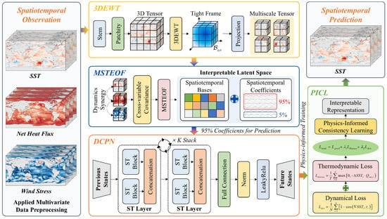
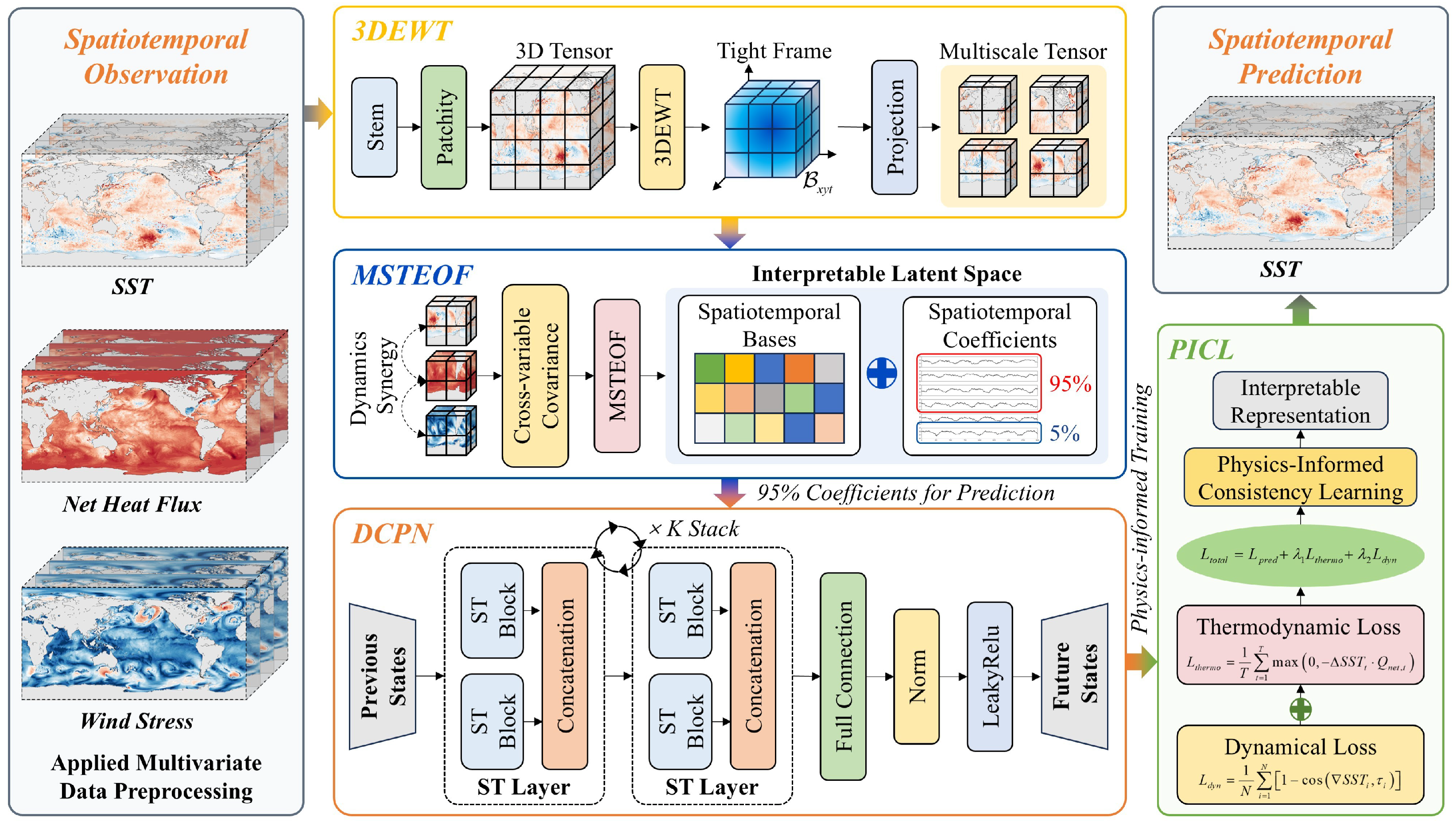
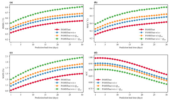
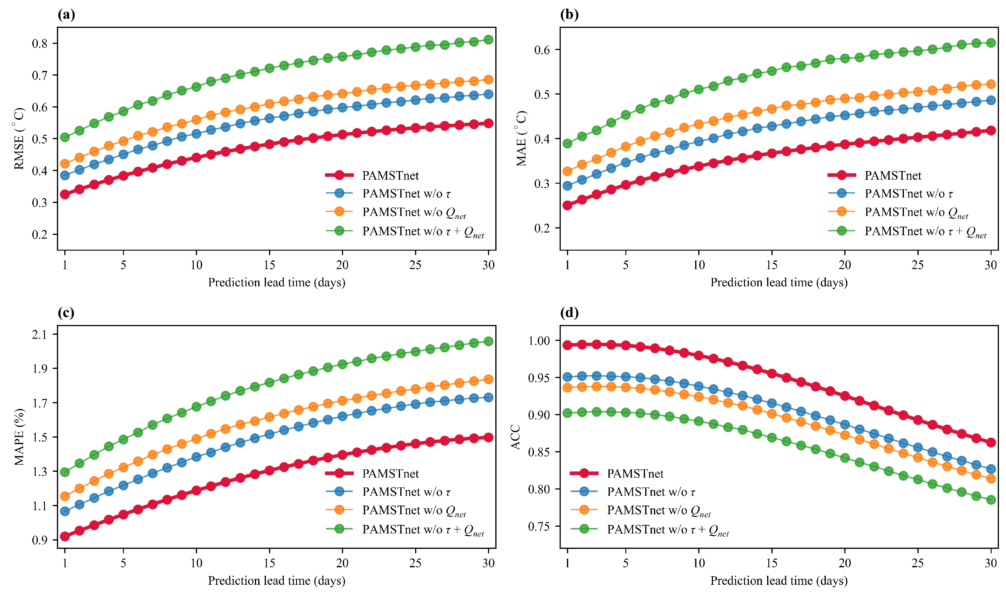
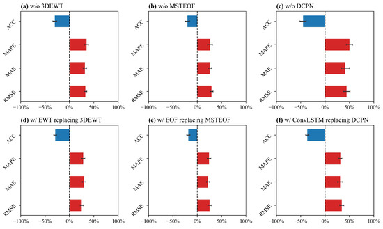
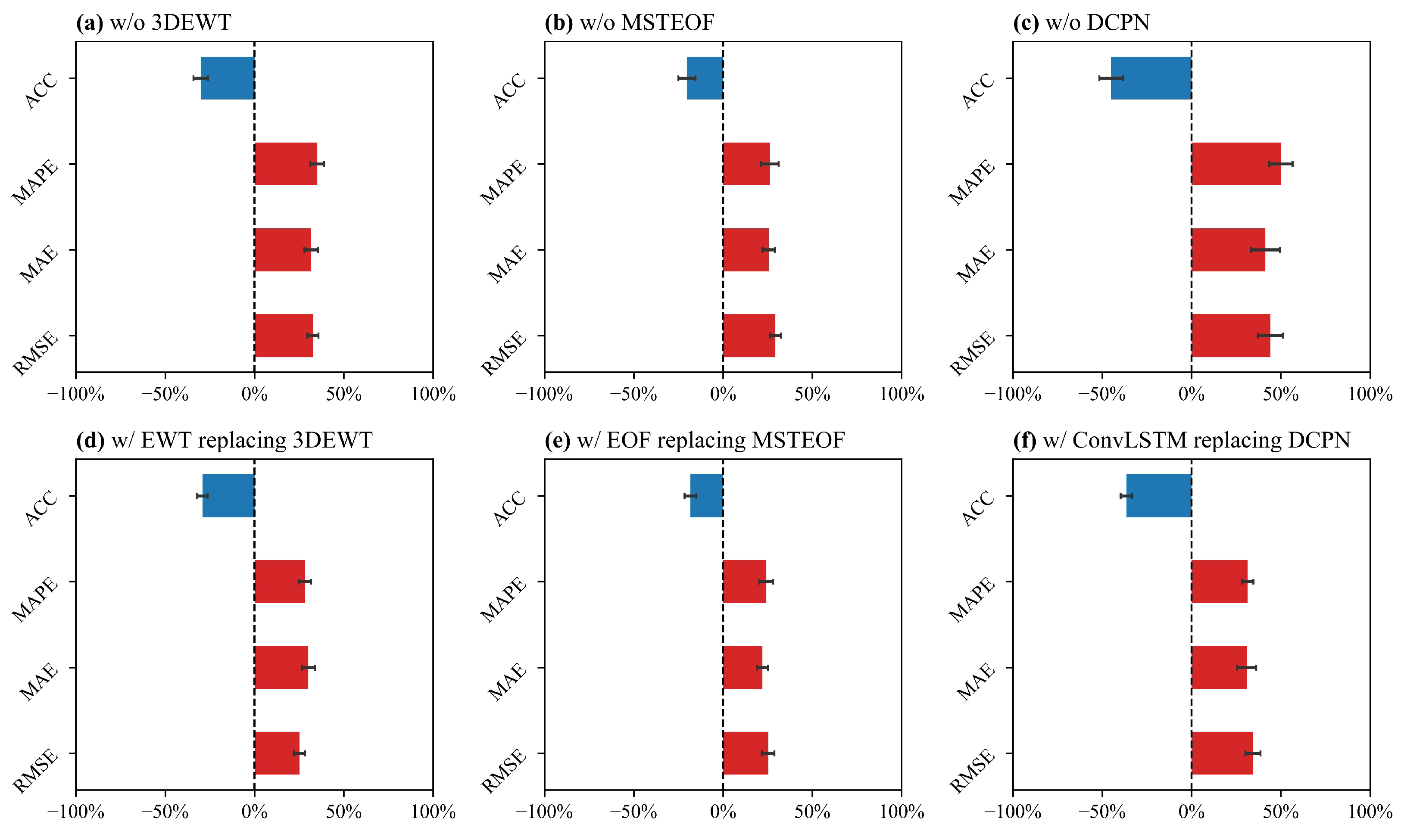
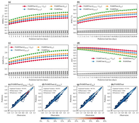
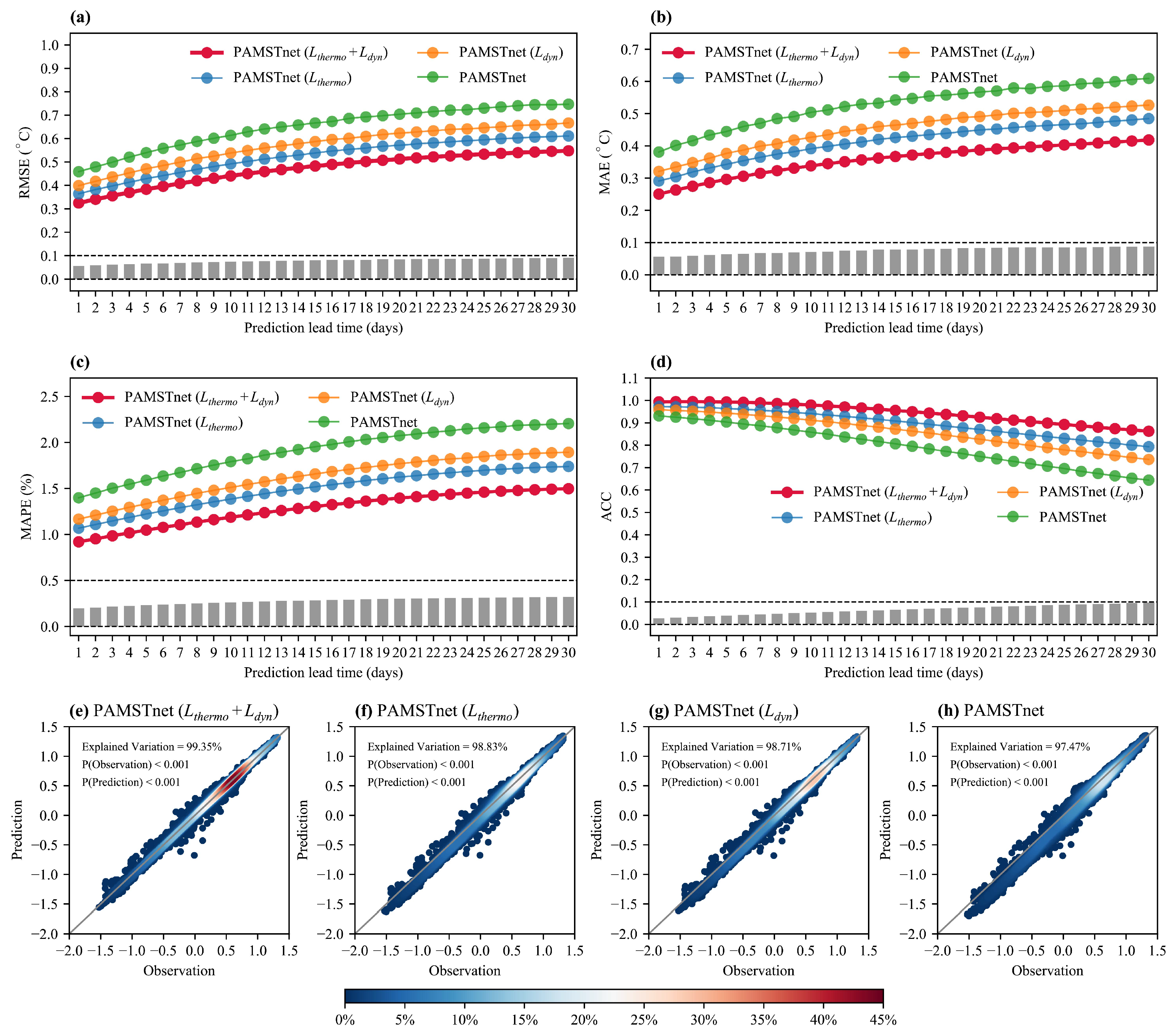
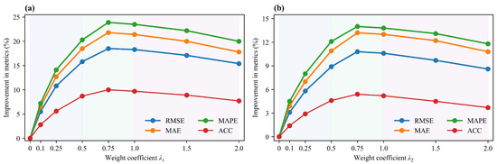
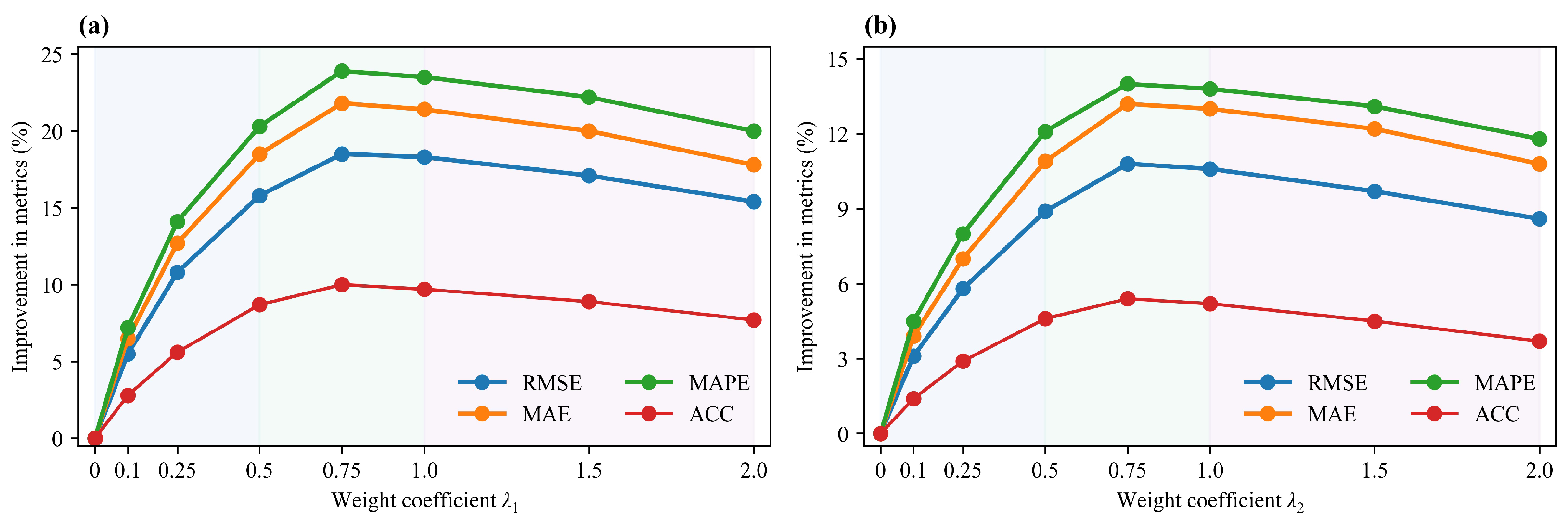
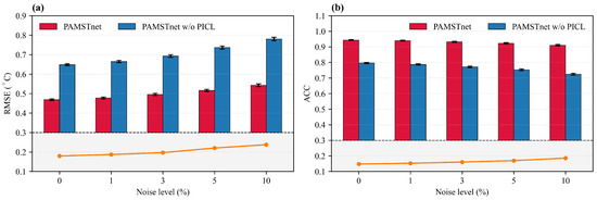
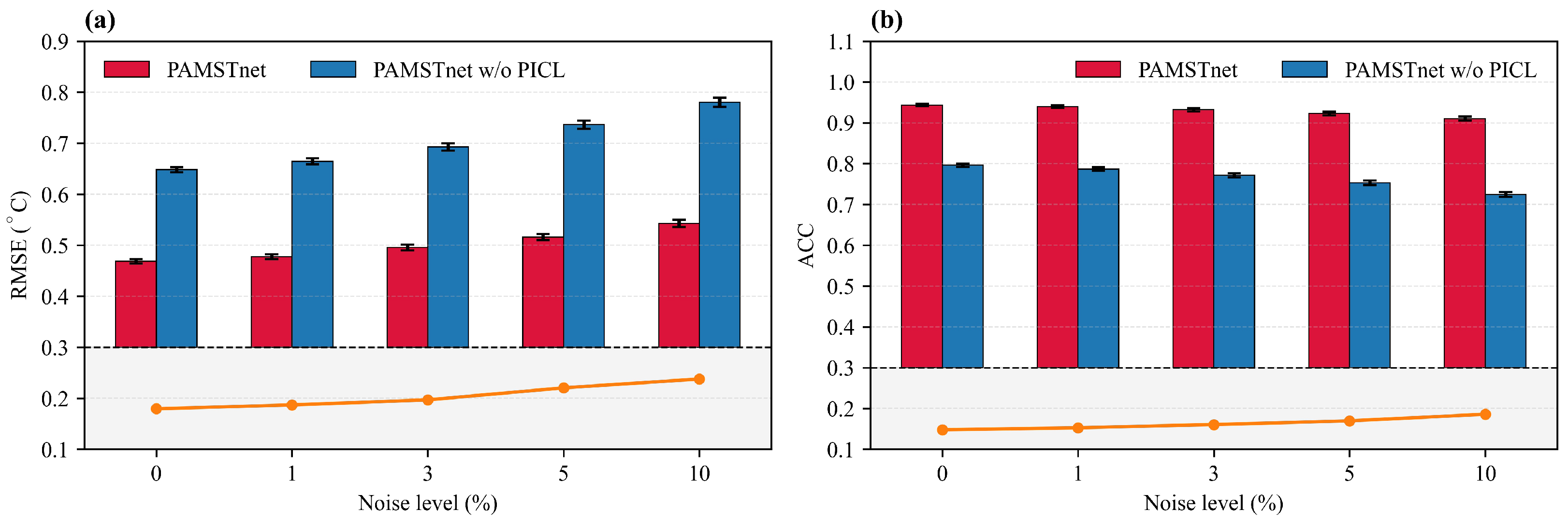
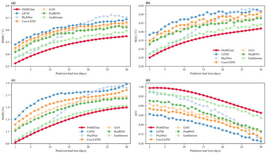
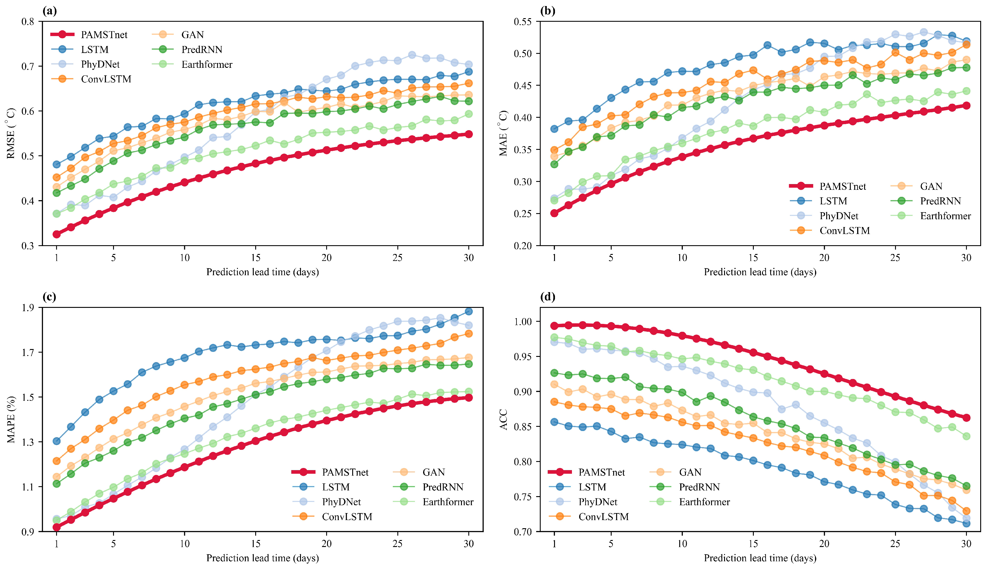
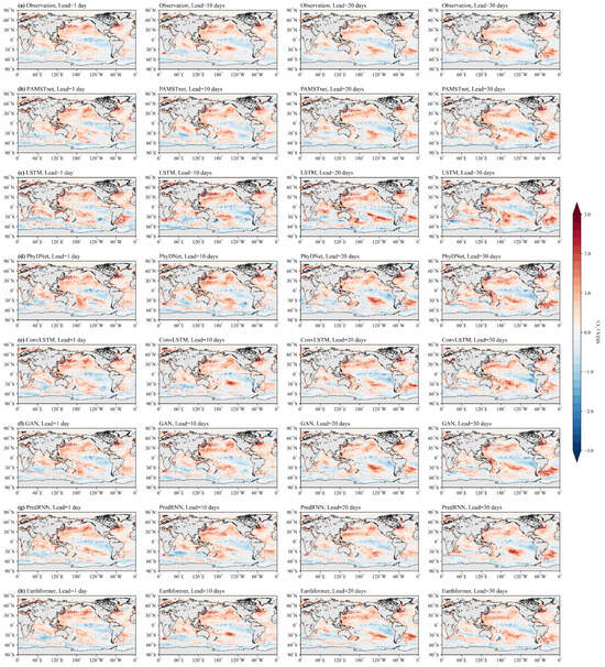
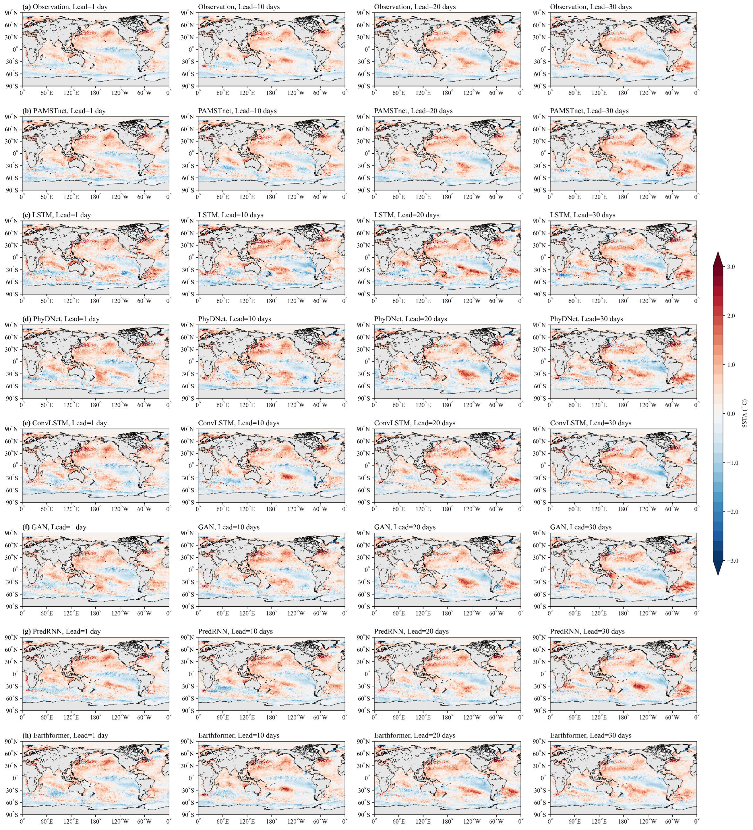
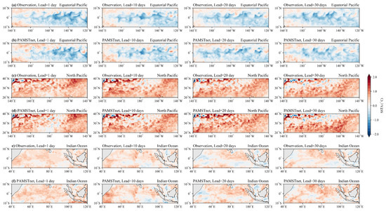
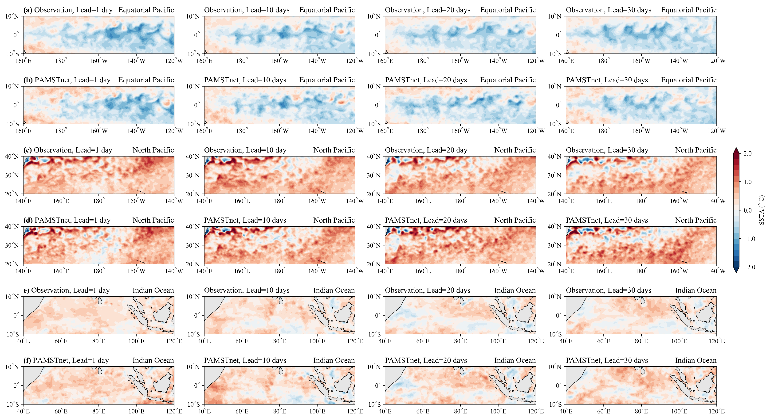
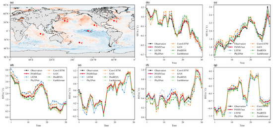
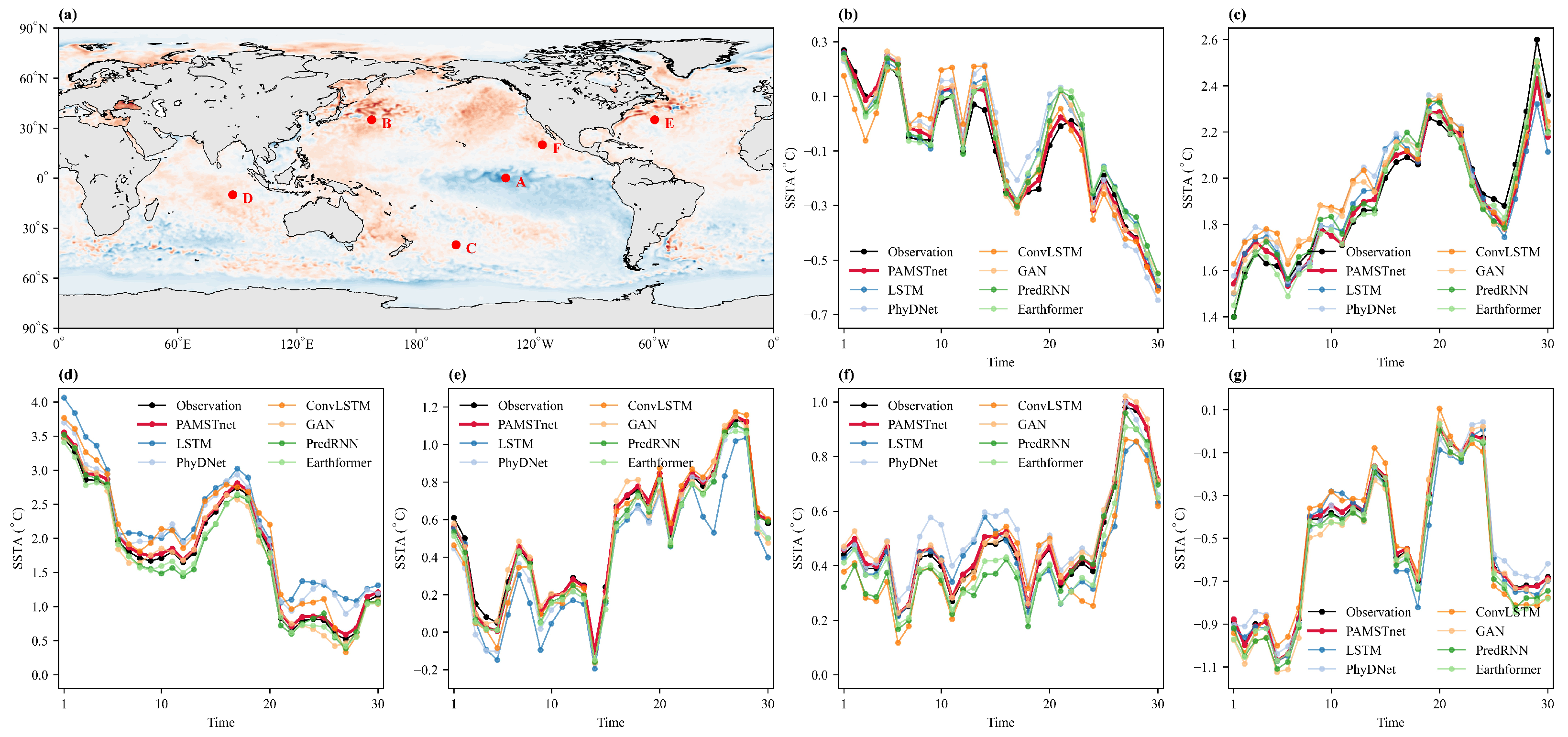
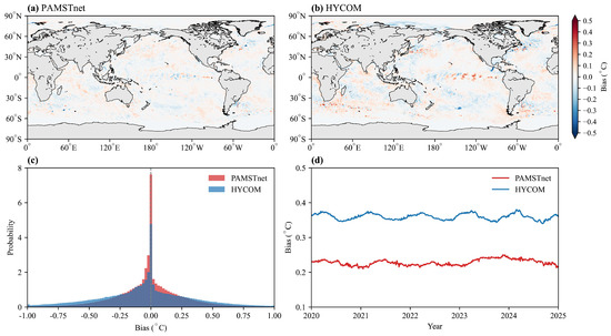
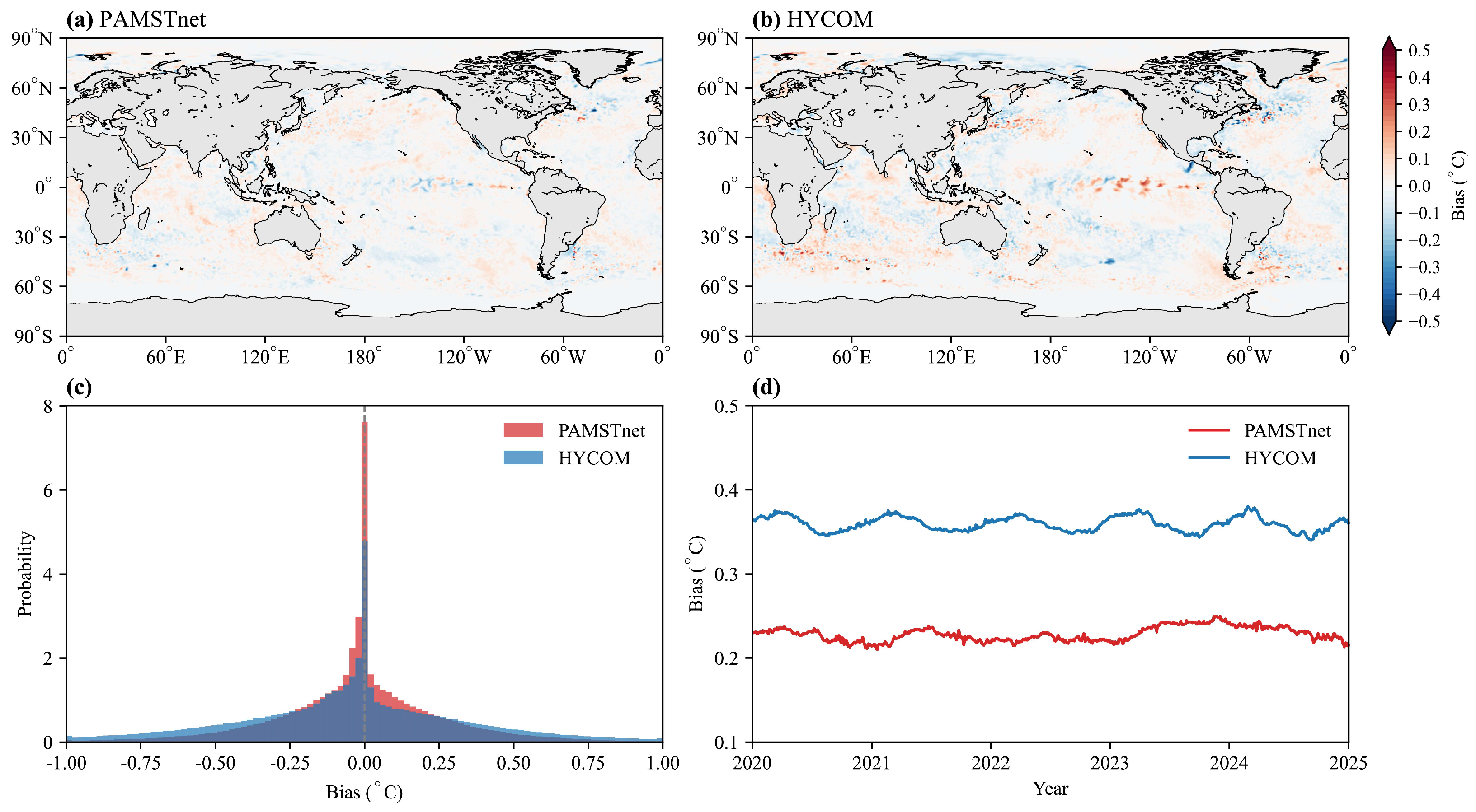
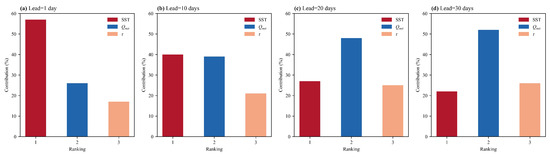
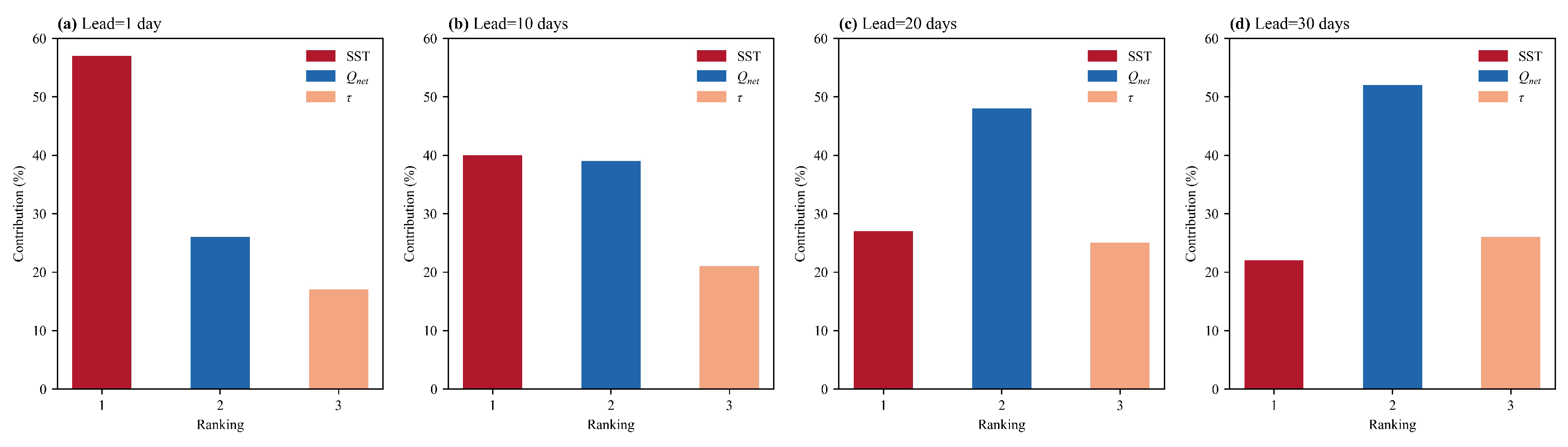
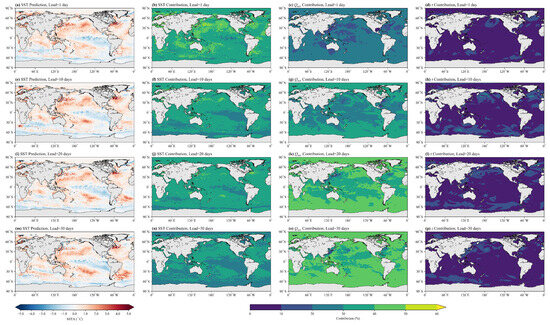
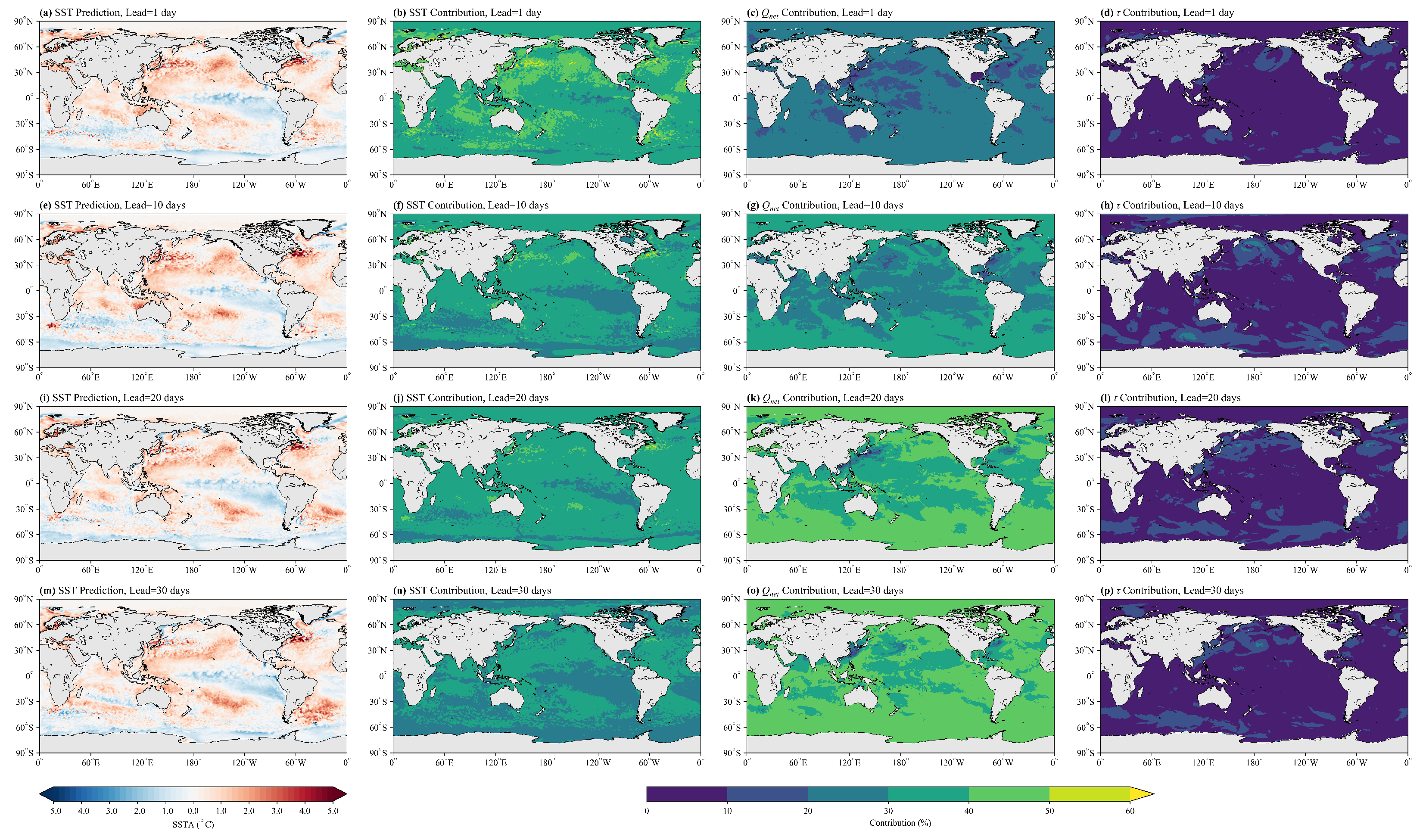
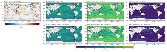
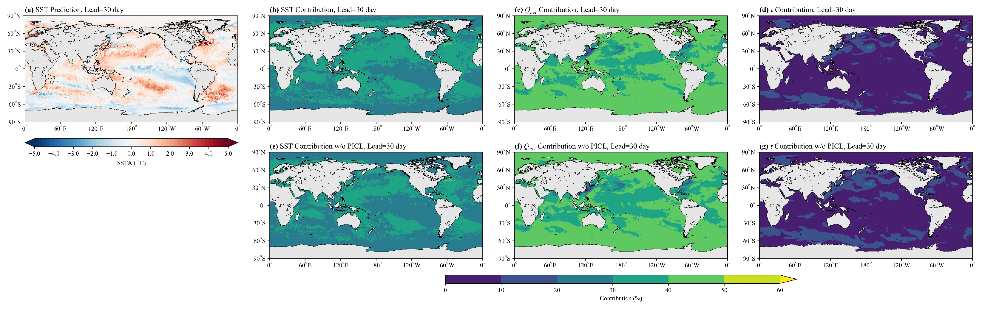
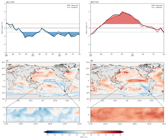
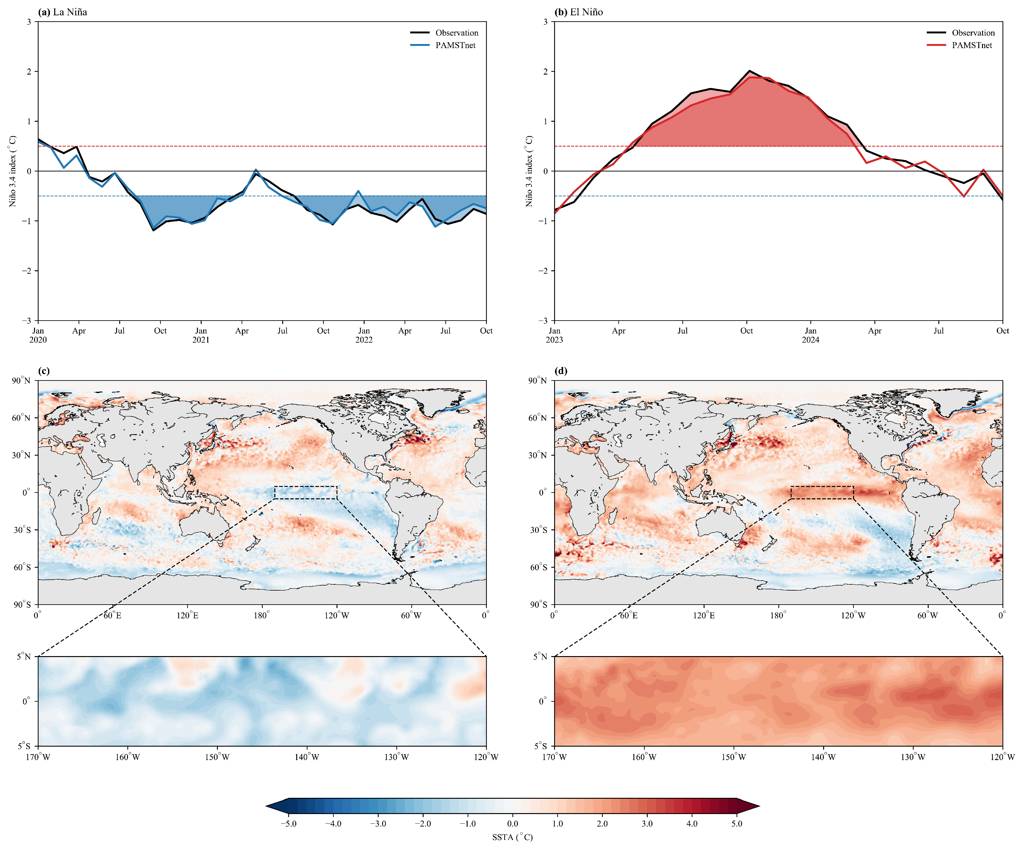

Disclaimer/Publisher’s Note: The statements, opinions and data contained in all publications are solely those of the individual author(s) and contributor(s) and not of MDPI and/or the editor(s). MDPI and/or the editor(s) disclaim responsibility for any injury to people or property resulting from any ideas, methods, instructions or products referred to in the content. |
© 2026 by the authors. Licensee MDPI, Basel, Switzerland. This article is an open access article distributed under the terms and conditions of the Creative Commons Attribution (CC BY) license.