


Highlights
What are the main findings?
- The Cubist model produced the best downscaling results.
- For the annual and monthly downscaled products, the downscaled data exhibited finer spatial patterns and eliminated the outliers present in the original data.
What are the implications of the main findings?
- The analysis reduces systematic bias and enhances the spatial descriptive capability of precipitation data.
- The downscaled dataset provides effective data support for hydrological and climate change research in the Qaidam Basin.
Abstract
High-spatiotemporal-resolution precipitation data are essential for studies on regional hydrology, meteorology, and ecological conservation. Because the Qaidam Basin is a data-scarce region with a few ground stations and coarse-resolution remote sensing products, its utility in regional research is constrained. Therefore, high-resolution precipitation data are urgently needed. Here, longitude, latitude, the normalized difference vegetation index (NDVI), the digital elevation model (DEM), daytime and nighttime land surface temperature, slope, and aspect were selected as environmental variables. Four machine learning methods, Artificial Neural Network (ANN), Cubist, Random Forest (RF), and Support Vector Machine (SVM), were used to downscale Tropical Rainfall Measuring Mission (TRMM) precipitation data from 25 to 1 km in the Qaidam Basin and validated using ground observation stations. For annual downscaling, the accuracy ranked as Cubist > ANN > RF > SVM, and residual correction further improved performance. The Cubist model produced the best results, generating finer spatial patterns and reducing outliers in both annual and monthly products. Longitude, latitude, the DEM, and the NDVI were important contributors to the Cubist model. The resulting high-resolution dataset provides valuable support for hydrological and climate change research in the Qaidam Basin.
1. Introduction
Precipitation is an important component of the global water cycle [1,2]. High-resolution, accurate precipitation data are among the foundational datasets for applications such as water resource management, meteorological disaster forecasting, and hydrological simulations [3,4]. Traditional methods of obtaining precipitation data include observations from ground meteorological stations and weather radar data. Although meteorological stations can provide high-accuracy data and high-spatial-resolution datasets can be derived through interpolation, the number of stations is limited, and their spatial distribution is uneven. This leads to interpolation errors, particularly in areas with sparse meteorological stations and complex terrains. Although weather radar can obtain precipitation data with high spatial resolution, it is susceptible to errors caused by factors such as climate and geographical environments [5,6]. The Qaidam Basin is a typical high-altitude, cold, and arid inland basin with frequent windblown sand, severe desertification, and a fragile ecological environment. The Qaidam Basin is located in a remote area with poor transportation infrastructure and sparse meteorological station coverage, making it a data-scarce region with challenges in capturing the heterogeneity of the spatial distribution of precipitation.
With the development of remote sensing technology, satellite remote sensing data has received increasing attention due to its advantages of broad observation coverage, sufficient spatiotemporal continuity, low cost, and real-time acquisition, and has become an important source for hydrometeorological research in data-scarce regions [7,8,9]. Various satellite precipitation products have been successively released, such as the Tropical Rainfall Measuring Mission (TRMM) [10], Global Precipitation Measurement (GPM) [11], Climate Prediction Center Morphing Technique (CMORPH) [12], and the Global Satellite Mapping of Precipitation Project (GSMaP) [13]. Because different study areas have different topographic and climatic conditions, satellite precipitation products perform differently across regions; therefore, selecting a precipitation product suited to the study area is particularly important. Zeng et al. [14] conducted a comparative evaluation of TRMM and GPM IMERG data based on in situ observations from the Qaidam Basin and found that, at the monthly and annual scales, TRMM data were 30% and 60% more accurate than GPM data, respectively. Moreover, TRMM data were able to capture the spatial distribution characteristic of higher precipitation in mountainous areas than in plains within the Qaidam Basin. Li et al. [15] used the Qinghai Lake Basin as the study area and compared the accuracy of TRMM, GPM, and CMORPH data; the results showed that TRMM data were more suitable for the study area than GPM data, while CMORPH data had the poorest suitability. Therefore, this study selected TRMM precipitation data, and the TRMM series of satellite precipitation products released by the National Aeronautics and Space Administration (NASA) are also among the most widely used precipitation products. However, the spatial resolution of these data (0.25°) is relatively low, making it difficult to meet the requirements for studying the spatiotemporal variability of precipitation at small and medium scales, limiting its application in driving hydrological and meteorological models within a basin [16]. Therefore, improving the spatial resolution of the TRMM precipitation products in the study area is of considerable importance.
The TRMM downscaling process primarily involves the selection of multisource environmental variables and the selection and improvement of downscaling models. The most widely used multisource environmental variables include the normalized difference vegetation index (NDVI), digital elevation model (DEM), latitude, and longitude [17,18]. In study areas with sparse vegetation, precipitation does not induce significant changes in the NDVI [3,19]. However, it causes variations in land surface temperature (LST) [20]. Therefore, in some studies, LST has been selected as an environmental variable and incorporated into downscaled models. Using these environmental variables, various downscaling models have been explored to obtain refined precipitation data. Linear regression models are commonly used for downscaling. Jia et al. [21] used the NDVI and DEM as environmental variables and applied a multi-source linear regression model to downscale TRMM precipitation data in the Qaidam Basin to successfully obtain high-resolution precipitation data. This model assumes a constant relationship between precipitation and environmental variables. However, the relationship between precipitation and environmental variables changes with spatial location [22]. To address this issue, Xu et al. [3] introduced a Geographically Weighted Regression (GWR) model to improve the downscaling algorithms. This algorithm incorporates the geographic location into the regression process, establishing a point-by-point relationship between environmental variables and precipitation to achieve downscaling. Downscaling based on the GWR model outperformed traditional regression models.
With the widespread application of machine learning techniques in the field of remote sensing and their advantages in handling complex nonlinear problems, these methods have been widely adopted for TRMM downscaling. Jing et al. [23] used two machine learning approaches, Random Forest and Support Vector Machine, to downscale TRMM precipitation data over the Qinghai–Tibet Plateau to a 1 km resolution. Both models exhibited high accuracy. Elnashar et al. [24] compared three machine learning methods for downscaling: Gradient Boosting Regressor (GBR), Support Vector Machine (SVM), and Artificial Neural Network (ANN). ANN achieved the best performance during the simulation process. Ma et al. [25] used Cubist, a spatial data mining algorithm, to downscale original TRMM data, obtaining results superior in accuracy to those yielded by GWR. Many studies have suggested that, on a monthly scale, vegetation responses to precipitation exhibit a certain delay and lag. For example, Duan et al. [16] argued that the response time of vegetation to precipitation data lags by two to three months. Therefore, in the downscaling of TRMM data, selecting an annual time scale is optimal.
However, different downscaling methods can yield different accuracy validation results within the same study area. Differences in topography, climate, and other factors among the study areas determine the complexity of the relationships between precipitation and environmental variables across regions. Therefore, the optimal method must be selected through validation against in situ observations. Given that the Qaidam Basin is influenced by both climate and complex terrain, and suffers from a scarcity of validation stations, classifying it as a data-sparse region, it is essential to analyze multiple downscaling methods in this area. Such an analysis aims to reduce systematic bias and enhance the spatial descriptive capability of precipitation data.
To optimize the spatial downscaling method applicable to TRMM precipitation products in the Qaidam Basin and estimate high-temporal and -spatial-resolution precipitation data, this study has two main objectives: (1) to establish downscaling models using four machine learning methods, Artificial Neural Network (ANN), Cubist, Random Forest (RF), and Support Vector Machine (SVM), to downscale annual TRMM data from 25 km to 1 km resolution and select the optimal model based on ground-based observation data; (2) to derive monthly precipitation data from the annual downscaled data using the proportional coefficient method and perform accuracy validation.
2. Study Area and Data
2.1. Study Area
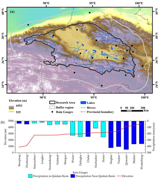
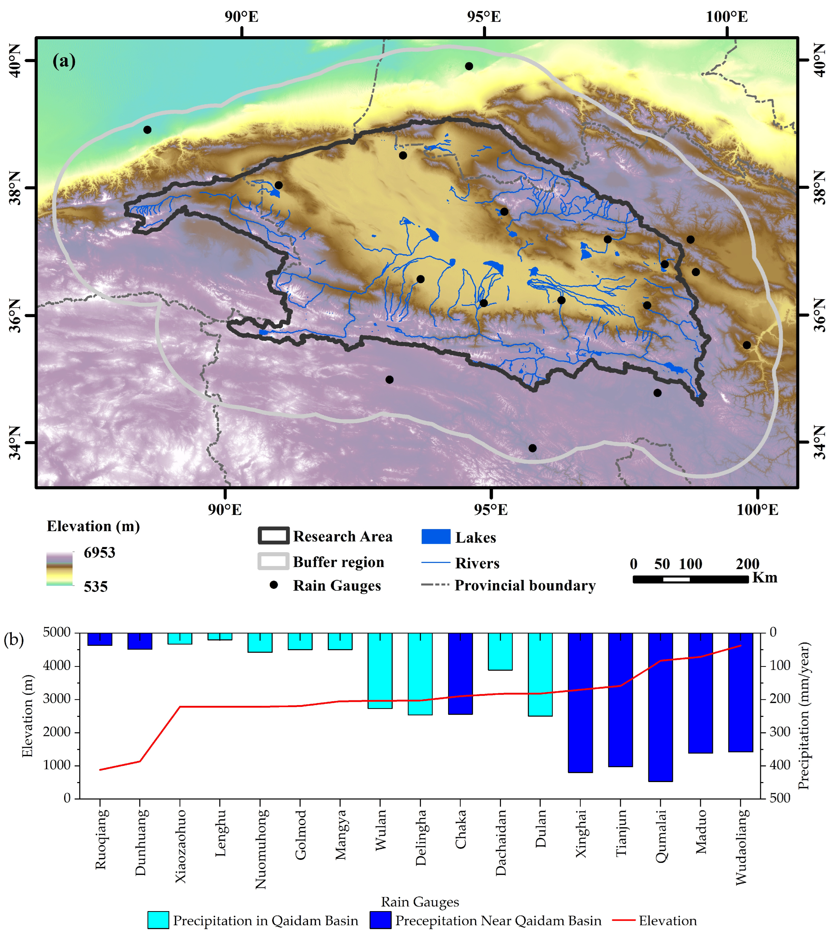
The Qaidam Basin is located in the northwest of Qinghai Province, China, covering an area of 90°16′ to 99°16′E and 35°00′ to 39°20′N (Figure 1a). It is bounded by the Altun Mountains to the northwest, the Qilian Mountains to the northeast, and the Kunlun Mountains to the south. It is the largest inland basin in China [26]. The basin covers an area of 275,000 km2 [27] and has an average altitude of over 3000 m. The basin lies at the interface between mid-latitude westerlies and the East Asian monsoon system within the arid region of northwestern China. It has a typical continental plateau climate characterized by cold and dry conditions, strong solar radiation, frequent winds, and generally less than 200 mm of precipitation. The total precipitation is generally below 200 mm, decreasing from the mountainous areas toward the interior of the basin, where it falls to less than 25 mm in the center. The main vegetation types in Qaidam Basin are steppes, shrublands, and deserts. The growing season extends from May to September each year, during which the monthly mean temperature is above 0 °C, and precipitation accounts for more than 90% of the annual total [28,29]. There are nine meteorological stations within the Qaidam Basin. They are mostly located in low-elevation plains where precipitation is low, with five stations having a mean annual precipitation below 100 mm (Figure 1b). There are virtually no meteorological stations in the high-elevation mountainous areas. To validate the accuracy of the downscaled results in mountainous regions, a 110 km buffer zone was established near the study area. Seventeen stations at different elevations were selected to validate the downscaled results.
Figure 1.
(a) Study area of the Qaidam Basin, and (b) annual average precipitation of 17 rain gauges within 0–5000 m elevation.
2.2. Data
2.2.1. TRMM Satellite Precipitation Dataset
The TRMM precipitation dataset was jointly developed by the NASA and the Japan Aerospace Exploration Agency, launched in November 1997. The TRMM is equipped with multiple sensors, and the three most critical sensors for precipitation measurement are the Precipitation Radar (PR), TRMM Microwave Imager (TMI), and Visible and Infrared Scanner (VIRS). The TRMM Multisatellite Precipitation Analysis (TMPA) algorithm retrieved precipitation estimates using information collected from multiple satellite sensors and ground-based rain-gauge networks, producing the best TRMM precipitation products. Initiated in 1998, the TMPA provides the near-real-time precipitation product TRMM 3B42RT and the non-real-time, rain-gauge-adjusted TRMM 3B42, covering the region between 50°N and 50°S globally, with a spatial resolution of 0.25° and a temporal resolution of 3 h. The TRMM 3B43 monthly precipitation dataset, which is widely used in research, was further adjusted based on 3B42 data [30]. The TRMM 3B43 (V7) monthly precipitation product used in this study was downloaded from the NASA website (https://daac.gsfc.nasa.gov/), covering the period from January 2000 to December 2019.
2.2.2. Terrain Dataset
The digital elevation model (DEM) was derived from the Shuttle Radar Topography Mission (SRTM) of NASA. We used SRTM data with a 90 m spatial resolution obtained from the Geospatial Data Cloud platform of the Computer Network Information Center, Chinese Academy of Sciences (https://www.gscloud.cn/). Based on these data, ArcGIS 10.8 software was used to derive additional topographic indices, including slope and aspect [31].
2.2.3. NDVI Datasets
The NDVI can accurately assess vegetation health and growth conditions, and numerous studies have shown that its spatiotemporal distribution is correlated, to some extent, with precipitation. This study used the MOD13A2 Version 6 dataset from January 2000 to December 2019 with a spatial resolution of 1 km and a temporal resolution of 16 days. NDVI time-series data are susceptible to factors such as sensor viewing angle, atmospheric conditions, and ice and snow, which can introduce outliers into the time series. To reduce noise, Savitzky–Golay filtering was applied to denoise raw data [32]. Based on these data, annual NDVI values were obtained by calculating the mean of the intra-annual NDVI observations.
2.2.4. LST Datasets
MODIS LST data provide observations for both daytime and nighttime. This study utilized the MOD11A2 Version 6 dataset with a spatial resolution of 1 km and a temporal resolution of 8 d. The annual mean daytime and nighttime land surface temperatures in the study area were calculated to derive the year-round daytime (LST-day) and nighttime (LST-night) land surface temperature datasets.
2.2.5. Rain Gauge Data
Ground observation station data used in this study were obtained from the China Meteorological Data Service Center (http://data.cma.cn/). The distribution of meteorological stations in the Qaidam Basin is shown in Figure 1. Stations within the study area were sparsely and unevenly distributed, with higher concentrations in the east and fewer in the west. Nine stations within the study area and eight adjacent stations to the study area were selected. Daily precipitation data from January 2000 to December 2019 were used.
3. Methods
3.1. Machine Learning Algorithms
In this study, we used four machine learning algorithms, namely, Artificial Neural Network (ANN), Cubist, Random Forest (RF), and Support Vector Machine (SVM), to downscale satellite precipitation data.
- (1)
- ANN is a mathematical model that simulates the behavior of biological neural networks composed of numerous interconnected nodes or neurons. This network can model the complex relationships between different variables [33]. ANN can be implemented through various approaches, among which the back-propagation neural network (BP-ANN) is the most widely used. The BP-ANN architecture consists of an input layer, one or more hidden layers, and an output layer. During modeling, it is necessary to determine the optimal number of nodes in the hidden layer, denoted as “hidden.”
- (2)
- Cubist is a rule-based linear regression decision tree model that uses an ensemble learning strategy. The rule sets contained within the model partitioned the sample set of the entire study area into subsets based on geographical attributes. These subsets are heterogeneous with respect to one another. Meanwhile, geographic attributes are homogeneous within the same subset. Within each subset, the relationship between precipitation and surface characteristics can be established using stepwise multiple linear regression [25,34]. In model construction, two key parameters must be specified, that is, the number of rules (committees) and the number of neighbors (neighbors).
- (3)
- RF is an ensemble machine learning model that uses the bootstrap method to randomly sample data with replacement, generating m training sets. Each of these new training sets is then used to construct a decision tree model [35]. The RF modeling process requires the determination of three critical parameters: a number of decision trees, ntree; a number of decision trees, mtry; and the number of nodes.
- (4)
- SVM is an algorithm based on statistical theory. It relies on a kernel function to map the input data into a high-dimensional space and construct an optimal hyperplane such that the error of all training samples relative to this optimal hyperplane is minimized, making predictions within an allowable error range [36]. To construct the model, a radial basis function (RBF) kernel was used, and the penalty factor cost and gamma coefficient were set.
The training and prediction of the research model were implemented in R 4.5.
3.2. Parameter Tuning
Parameter tuning of machine learning algorithms plays a crucial role in model accuracy. The parameters of the four machine learning algorithms used in this study are listed in Table 1. To construct optimal models, we used the ten-fold cross-validation method to determine the best parameter values for each machine learning algorithm [37,38]. Specifically, all 25 km samples were randomly divided into 10 subsets, with 9 subsets used as the training dataset and the remaining 1 subset used as the test dataset. This process was repeated ten times until each subset was used for both the training and test datasets. Model performance was evaluated based on the average of ten Root Mean Square Error (RMSE) values [39].
Table 1.
Parameter ranges for four machine learning algorithms.
3.3. Main Downscaling Steps
- (1)
- In areas covered by lakes, rivers, and ice/snow, NDVI values generally remained constant and exhibited no correlation with precipitation. Therefore, raster data values for such regions should be excluded. Consequently, we removed pixels representing water bodies and ice/snow, specifically those with NDVI values less than 0, from the 1000 m resolution NDVI dataset. The relationship between precipitation and the NDVI can be distorted by irrigation, harvesting, and soil moisture, leading to anomalous NDVI values. To mitigate the interference of these factors, a low-pass filter was used to identify and eliminate outliers [3,40]. The algorithm is as follows.where S_NDVI1km(u) represents the difference before and after filtering at pixel u, and NDVI1km(u) represents the original NDVI value at pixel u. In this study, an 11 × 11 moving window is selected. However, this parameter can be adjusted for different study areas based on an assessment of natural and anthropogenic factors.
- (2)
- The 1 km spatial resolution data were resampled, including the NDVI, the DEM, longitude, latitude, LST-d, LST-n, slope, and aspect, to a 25 km spatial resolution using the mean value method, and the longitude and latitude information for the corresponding grid cells were extracted.
- (3)
- A machine learning model was used to establish the correlation between TRMM data and environmental variables at 25 km resolution. Ten-fold cross-validation was employed to tune the model parameters and determine the optimal model.
- (4)
- At a spatial resolution of 25 km, the model trained in Step (3) was used to predict the annual precipitation and simulate the total annual precipitation for each year.
- (5)
- The residuals between the original satellite precipitation data and the predicted precipitation at 25 km resolution were computed, and the residuals were interpolated to a 1 km resolution.
- (6)
- The 1 km spatial resolution environmental variables were input into the trained model to generate an annual precipitation product at a resolution of 1 km.
- (7)
- The 1 km precipitation data from Step (6) to the residual data from Step (5) were added to obtain the final downscaled precipitation data at a 1 km spatial resolution.
3.4. Monthly Precipitation Downscaling Study
Given the lagged response of vegetation to precipitation, we used the proportional coefficient method to derive monthly precipitation from annual precipitation data. The proportional coefficients were calculated as the ratio of monthly satellite precipitation at the original resolution to the corresponding annual precipitation, decomposing the 1 km resolution annual precipitation data into monthly precipitation [16]. The steps for the monthly precipitation downscaling are as follows:
- (1)
- Calculate the proportional coefficient of monthly precipitation relative to the corresponding year (Fractioni):where Fractioni denotes the proportionality coefficient for the ith month, OrgSat_Prei represents the amount of precipitation from the original satellite precipitation data for the ith month of the corresponding year, and the denominator indicates the cumulative annual precipitation for that year.
- (2)
- Use kriging interpolation to interpolate Fractioni to a 1 km spatial resolution, obtaining proportional coefficients at the same resolution as the annual downscaled precipitation data.
- (3)
- Multiply the 1 km annual downscaled precipitation by the 1 km resolution proportionality coefficient:where Mon_ represents the monthly precipitation data at 1 km resolution for the ith month, Fraction 1 denotes the interpolation-derived scaling factor at 1 km resolution for the ith month, and Sat_ corresponds to the downscaled annual precipitation data at 1 km resolution.
3.5. Validation
To evaluate the validity of the original satellite precipitation data and the downscaled results for the Qaidam Basin, three metrics were selected for accuracy assessment: the coefficient of determination (R2), root mean squared error (RMSE), and mean absolute error (MAE). This selection was based on satellite precipitation accuracy verification methods widely used in previous studies [3,21].
where O denotes the measured precipitation data from the ground observation station, and P denotes the estimated precipitation value for the grid cell corresponding to the ground observation station.
4. Results
4.1. Analysis of TRMM Annual Downscaling Results
4.1.1. Accuracy Verification of Annual Downscaling Results from Different Models
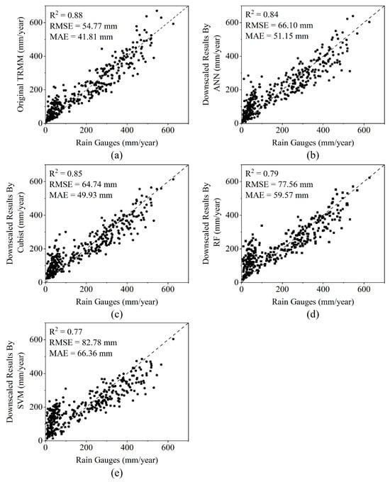
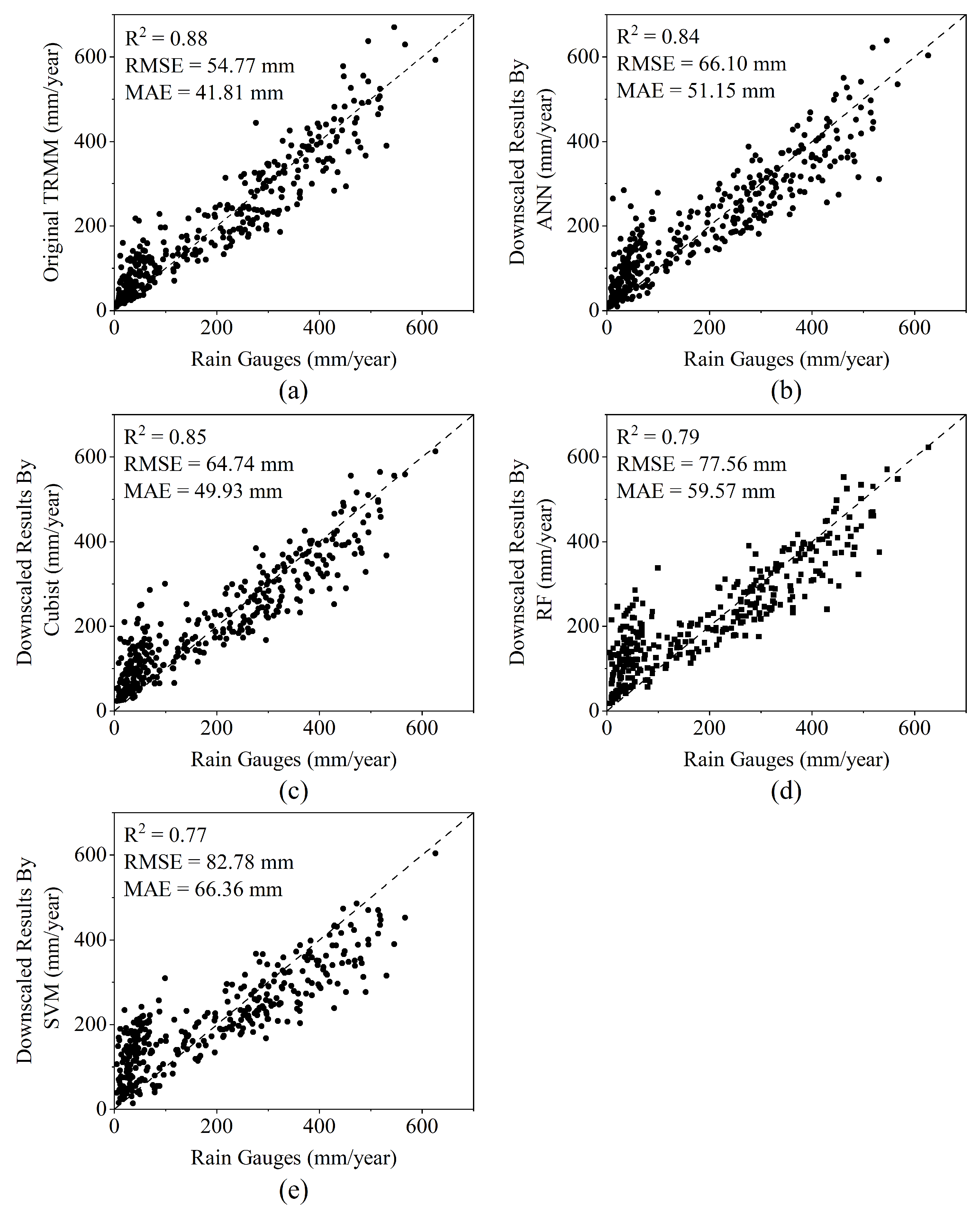
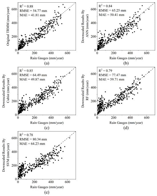
To compare and validate the annual TRMM precipitation data against 1 km downscaled data derived from four machine learning models, we used observational data from 17 ground meteorological stations within and surrounding the Qaidam Basin to verify the accuracy of the precipitation datasets. Figure 2 shows scatter plots comparing the original TRMM data and downscaled precipitation data before residual correction generated by the different algorithms against the observed data.
Figure 2.
Scatterplots of precipitation measured at rain gauges versus (a) TRMM data and downscaled data based on (b) ANN, (c) Cubist, (d) RF, and (e) SVM models, before residual correction in the Qaidam Basin.
Based on the validation results, the original TRMM data achieved the highest accuracy (R2 = 0.88; RMSE = 54.77 mm; MAE = 41.81 mm). Among the four downscaling methods, before residual correction, the precipitation data derived from the Cubist model demonstrated the highest accuracy (R2 = 0.85; RMSE = 64.74 mm; MAE = 49.93 mm), followed by the ANN model (R2 = 0.84; RMSE = 66.10 mm; MAE = 51.15 mm). The accuracy of the downscaled data retrieved by these two methods was comparable. The downscaling results based on the RF and SVM models were less accurate, and both had R2 below 0.8. Their RMSE values exceeded those of the ANN and Cubist downscaling results by more than 10 mm. Their MAE values were higher by more than 5 mm. The downscaled data derived from the SVM model exhibited the lowest accuracy.
Figure 3 shows the scatter plots of the precipitation data after residual correction, following downscaling by different algorithms, versus the observed data. The accuracy of the downscaled data from all four machine learning algorithms improved after residual correction. In terms of the degree of improvement, the ANN, Cubist, and RF algorithms showed only marginal gains in accuracy after residual correction. Their coefficients of determination (R2) remained unchanged, and the RMSE and MAE values differed little from those before correction. Conversely, the accuracy of the downscaled SVM data improved significantly. The residual-corrected downscaled data were used for analysis in subsequent studies.
Figure 3.
Scatterplots of precipitation measured at rain gauges versus (a) TRMM data and downscaled data based on (b) ANN, (c) Cubist, (d) RF, and (e) SVM models, after residual correction in the Qaidam Basin.
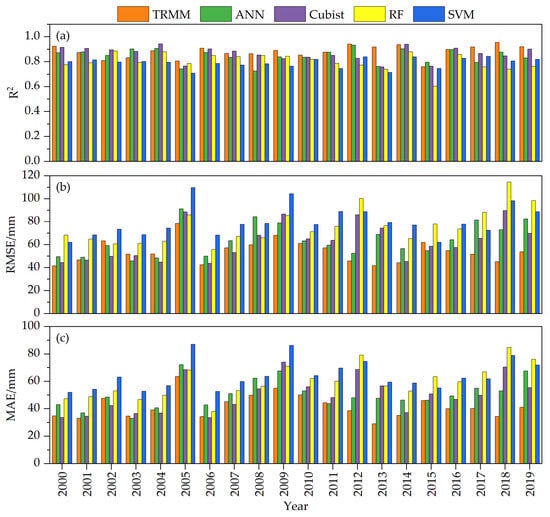
To further analyze the performance of the four downscaling models across individual years, the annual downscaled results were validated for each year from 2000 to 2019 using observed station data. The annual accuracy assessment results are shown in Figure 4. In terms of R2, the original TRMM data exhibited the highest correlation with the observations, with a multi-year mean of 0.88; R2 reached a maximum of 0.95 in 2018 and a minimum of 0.76 in 2015. Among the four downscaling model outputs, the Cubist-based model had the highest R2, with a multi-year mean of 0.86; it peaked at 0.94 in 2004 and dropped to a minimum of 0.76 in 2013. The ANN-based model showed an R2 similar to that of the Cubist model, with a multi-year mean of 0.85; it reached a high of 0.93 in 2012 and a minimum of 0.73 in 2008. RF and SVM had lower mean R2 values of 0.80 and 0.79, respectively, with R2 ranges of 0.60–0.88 and 0.71–0.84.
Figure 4.
(a) R2, (b) RMSE, and (c) MAE for TRMM data and downscaled results from different algorithms compared with precipitation measured at rain gauges from 2000 to 2019.
In terms of RMSE, the original TRMM data achieved the highest accuracy against the observed stations, with a multi-year mean of 53.94 mm. Among the four downscaling model results, the Cubist model was the most accurate, with a multi-year mean RMSE of 62.60 mm, while the ANN model was slightly less accurate than Cubist at 63.84 mm. The RF and SVM models had the lowest accuracy, with multi-year mean RMSEs of 76.01 mm and 79.82 mm, respectively.
In terms of MAE, the original TRMM data had the highest accuracy, with a multi-year mean of 41.81 mm. Among the four downscaling model results, the Cubist model had the highest accuracy, with a multi-year mean MAE of 49.87 mm; the ANN model was similar to Cubist at 50.41 mm. The RF and SVM models had the lowest accuracy, with multi-year mean MAEs of 59.71 mm and 64.23 mm, respectively.
4.1.2. Spatial Distribution of Annual Downscaling Results from Different Models
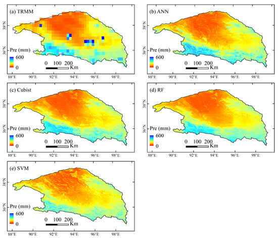
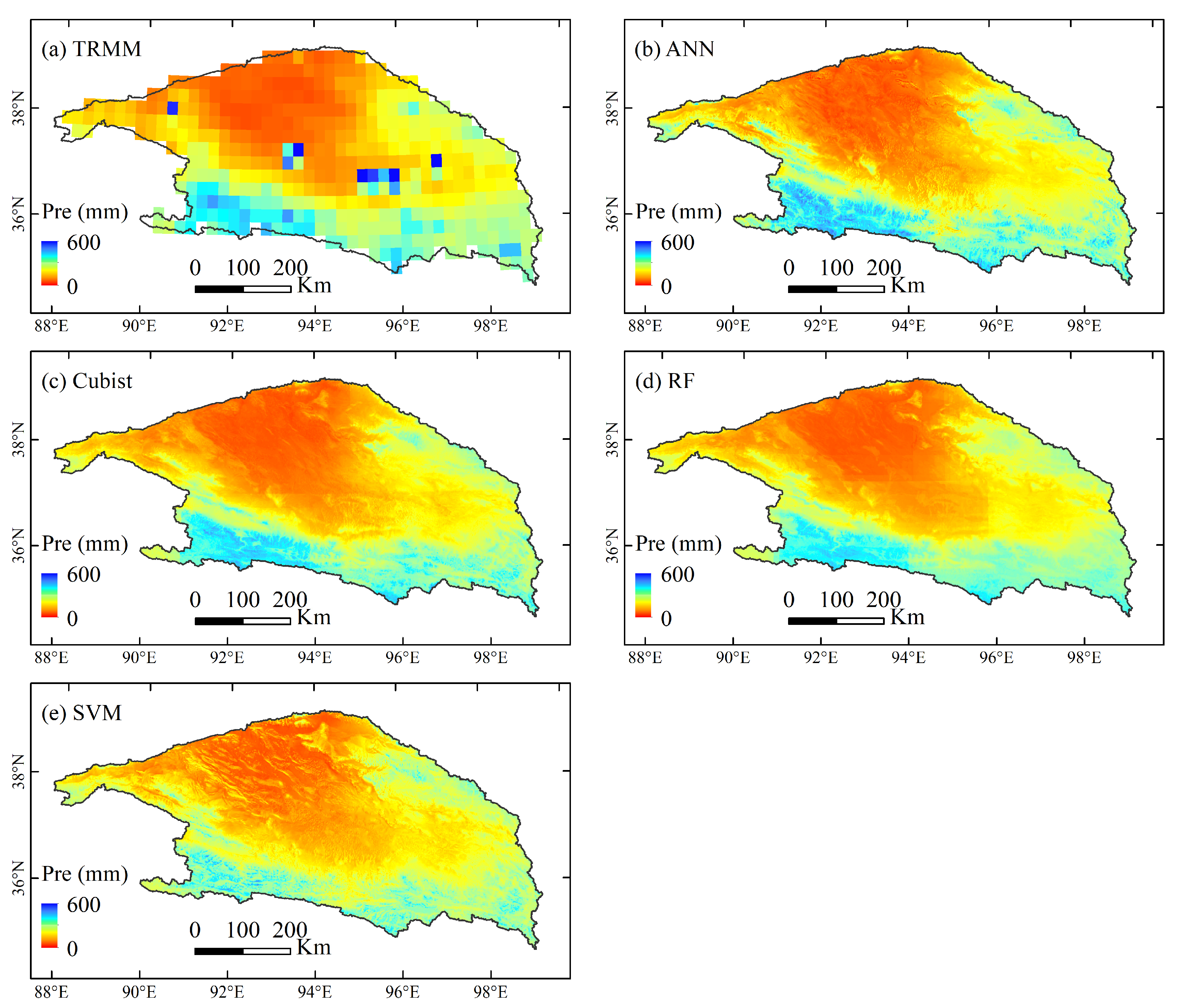
Figure 5 illustrates the spatial distribution of the original TRMM precipitation data and the 1 km annual precipitation data downscaled by the four machine learning models for the Qaidam Basin, using 2010 as a case study. The downscaled precipitation data derived from the four models exhibited a spatial distribution similar to that of the original TRMM data. Precipitation levels were higher in the eastern and southern regions of the Qaidam Basin. Meanwhile, the central and northwestern regions showed lower precipitation. The downscaled data based on the ANN, Cubist, and RF models are relatively smooth, whereas the downscaled data based on the SVM model appear spatially fragmented. Meanwhile, the inversion algorithm of the original TRMM data is affected by the underlying surface and has anomalies [41], especially in the water bodies of alpine mountainous areas. For example, the precipitation estimation values of Toson Lake and Hurleg Lake in the eastern Qaidam Basin are significantly higher than those in the surrounding areas, while the precipitation grid points of Dabsan Lake in the central part and Gas Lake in the western part are obviously overestimated compared with the surrounding precipitation data. In contrast, the downscaling data based on the four machine learning models eliminates these anomalies of the original TRMM data and is closer to the actual precipitation. Although the downscaled data based on the four machine learning algorithms were slightly less accurate than the original TRMM data, they provided higher spatial resolution and captured more specific and accurate precipitation details. And more importantly, they removed the anomalous points present in the original data.
Figure 5.
Spatial distribution of (a) TRMM data and downscaled data based on (b) ANN, (c) Cubist, (d) RF, and (e) SVM models in the Qaidam Basin in 2010.
4.2. Analysis of TRMM Monthly Downscaling Results
4.2.1. Accuracy Verification of Monthly Downscaling Results from Different Models
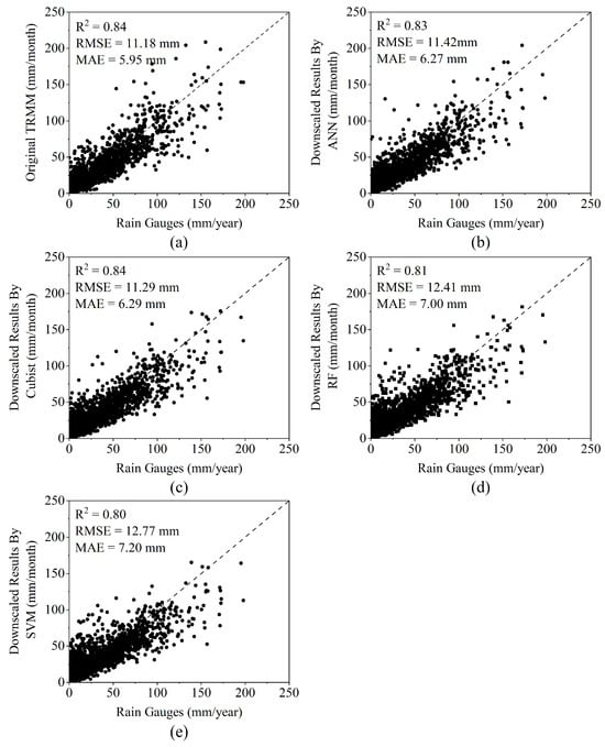
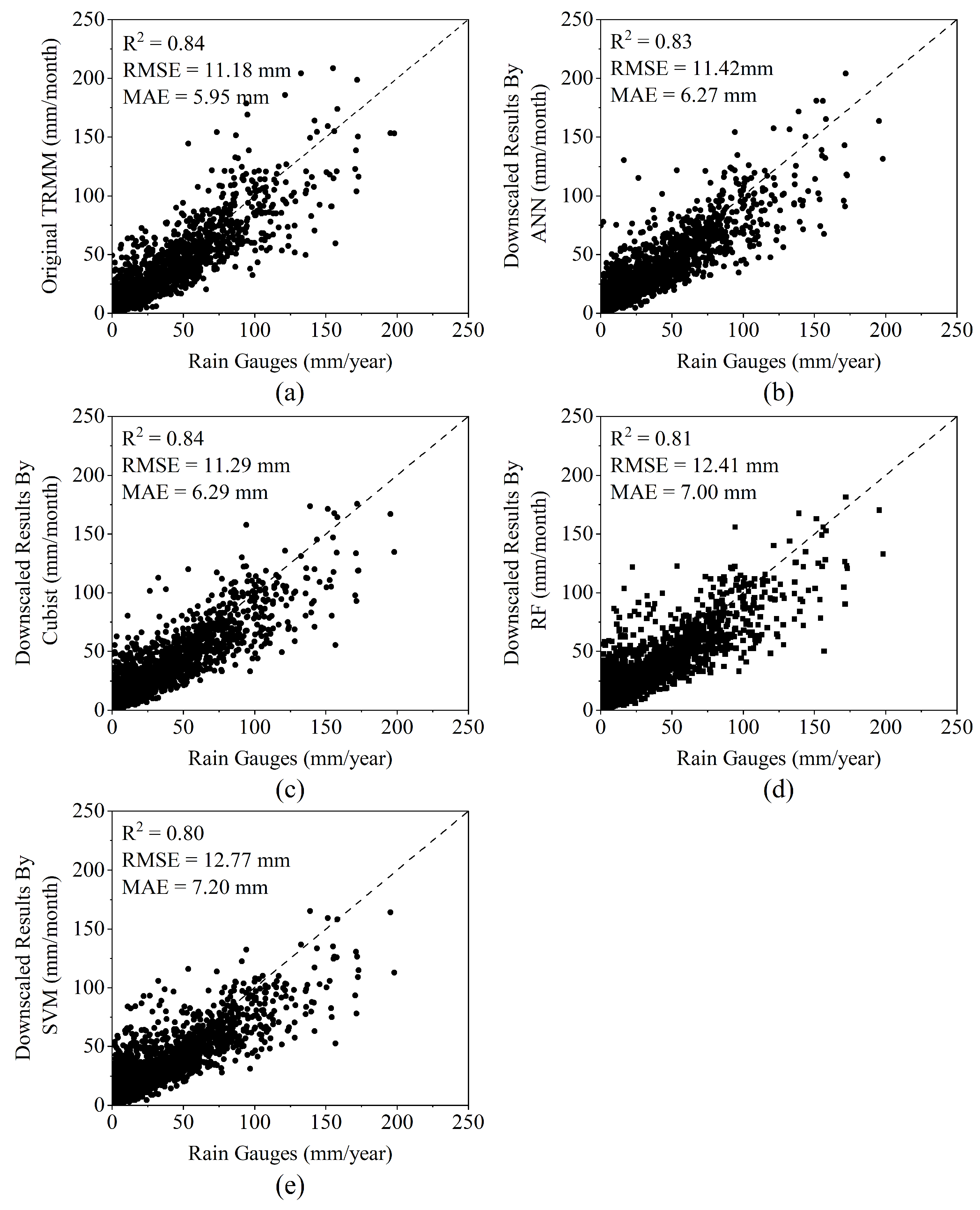
Based on the 1 km annual downscaled data, we applied the proportional coefficient method to disaggregate annual precipitation into monthly precipitation. Using monthly ground-based observations from the Qaidam Basin and its surrounding areas, we validated the accuracy of the original monthly TRMM data and the downscaled results produced by the four machine learning algorithms. The results are shown in Figure 6. The original TRMM data exhibited the highest accuracy (R2 = 0.84; RMSE = 11.18 mm; MAE = 5.95 mm). In the accuracy validation of the four monthly downscaled datasets, in terms of the R2, the Cubist-based downscaled dataset had the highest value at 0.84, followed by the ANN model at 0.83. In terms of the RMSE, the Cubist-based downscaled dataset performed best at 11.29 mm, followed by the ANN model at 11.42 mm. In terms of the MAE, the ANN-based downscaled dataset performed best at 6.27 mm, followed by the Cubist model at 6.27 mm. The monthly downscaled datasets based on the ANN and Cubist models exhibited the highest accuracy with only minor differences between them. The downscaled datasets based on the RF and SVM models showed lower accuracy.
Figure 6.
Scatterplots of the monthly (a) TRMM data and downscaled data based on the (b) ANN, (c) Cubist, (d) RF, and (e) SVM models versus precipitation measured at rain gauges after residual correction in the Qaidam Basin.
To further compare and analyze the accuracy of the original TRMM data and the downscaled data for each month from January to December, accuracy validation was conducted for the datasets based on monthly ground observation data from 2000 to 2019. The validation results are presented in Table 2. The original TRMM data exhibit the highest accuracy. Among the four accuracy validations of the monthly downscaled data, the downscaled data produced by the Cubist model achieved the highest coefficient of R2. From the perspective of temporal variation, the correlation coefficient first increased and then decreased. December had the lowest correlation coefficient, whereas all the other months had correlation coefficients greater than 0.5. September and October had the highest correlation coefficients, exceeding 0.8. The temporal variation patterns of the RMSE and MAE were broadly consistent, with the values showing a trend of first increasing and then decreasing. For the RMSE, the Cubist model downscaled data likewise had the highest accuracy: RMSE values from May to September were greater than 10 mm, reaching a maximum of 21.85 mm in July, and less than 10 mm in the remaining months. For the MAE, the ANN model downscaled data had the highest accuracy: MAE values from June to September were greater than 10 mm, reaching a maximum of 12.07 mm in July, and less than 10 mm in the remaining months.
Table 2.
Monthly validation results of TRMM data and downscaling results from different algorithms.
4.2.2. Spatial Distribution of Monthly Downscaling Results
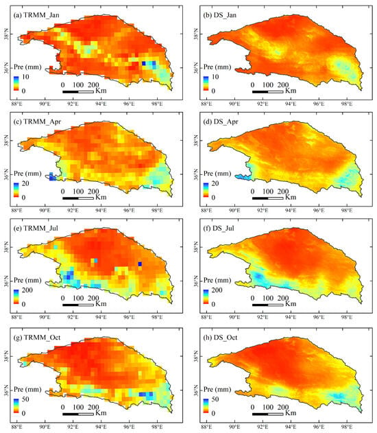
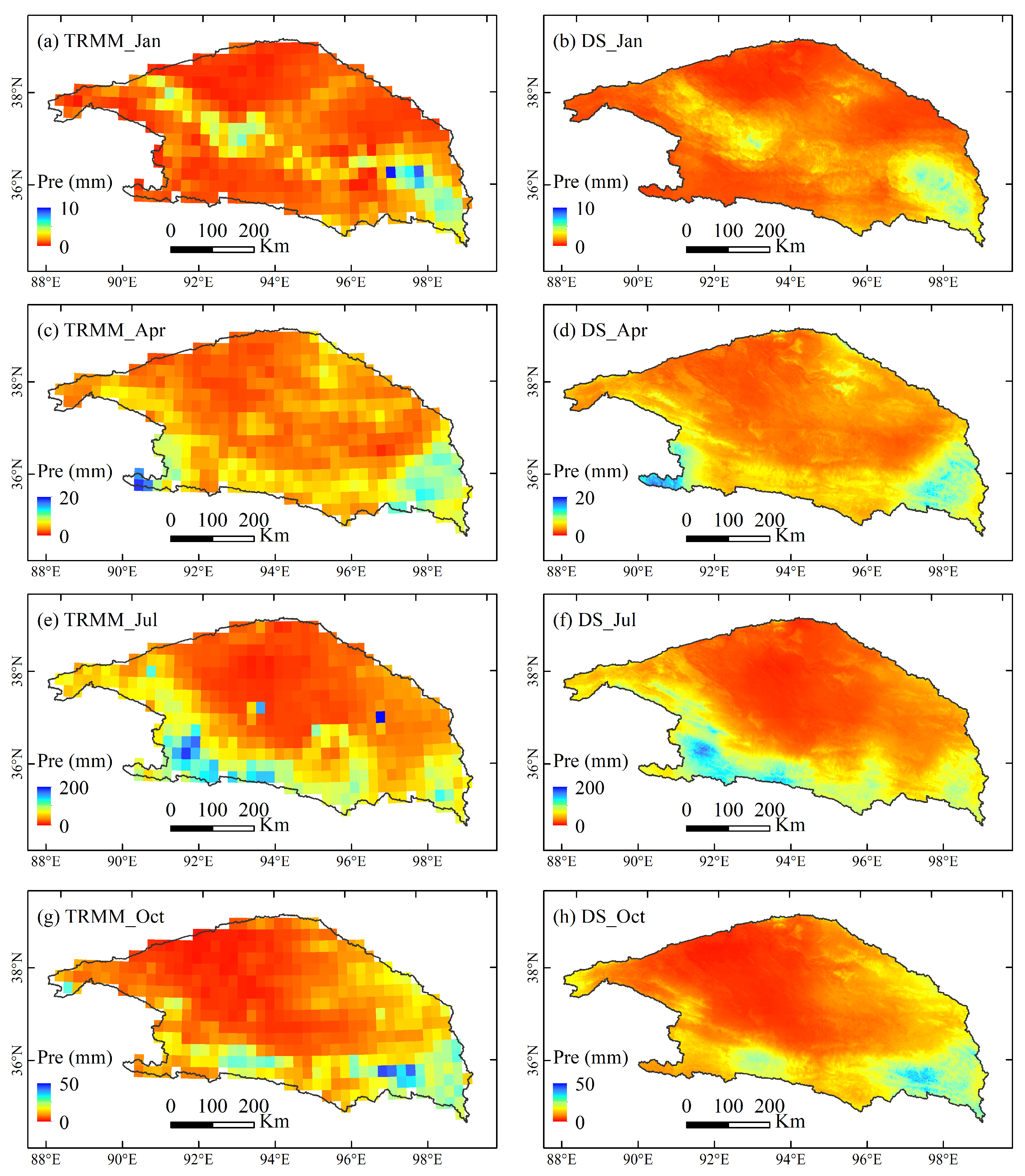
Based on the accuracy validation results, we selected the monthly downscaled data generated by the Cubist model to examine the spatial distribution patterns. Taking 2010 as an example, the original TRMM data and downscaled data for January, April, July, and October were compared to represent the different seasons. The results are shown in Figure 7. The downscaled precipitation data exhibited a spatial distribution similar to that of the original TRMM data. Although the downscaled data were slightly less accurate than the original TRMM data, the downscaled precipitation data had a smoother spatial distribution. They removed outliers and revealed more detailed precipitation information, thereby providing a robust data foundation for hydrological research in the Qaidam Basin.
Figure 7.
Spatial distribution of Tropical Rainfall Measuring Mission (TRMM) data and downscaled (DS) data in the Qaidam Basin: (a) TRMM data in January, (b) downscaled data in January, (c) TRMM data in April, (d) downscaled data in April, (e) TRMM data in July, (f) downscaled data in July, (g) TRMM data in October, and (h) downscaled data in October.
5. Discussion
5.1. Comparison of Machine Learning Models
Among the four machine learning algorithms used in this study, the Cubist model produced the best precipitation downscaling results at both annual and monthly scales, followed by the ANN model. At both annual and monthly scales, the downscaling results of the ANN and Cubist models exhibited certain similarities in accuracy validation, indicating that both models are capable of capturing complex nonlinear relationships within the dataset and have a certain applicability in the Qaidam Basin. In contrast, the RF and SVM models showed poorer downscaling accuracy. In different studies, the optimal model chosen by researchers also varies; some scholars have argued that the ANN model performs better [42], or that the RF model performs better [37]. Given the complexity of the relationships between environmental variables and precipitation, the performance of different machine learning methods should be compared when conducting downscaling in the study area. Based on the accuracy validation and spatial distribution of the annual and monthly downscaling results of each model, this study finally selected the Cubist model. On the other hand, the Cubist model is a divide-and-conquer spatial data-mining algorithm that partitions the study area into different subregions, within which geo-graphic attributes are consistent, and constructs regression relationships between precipitation and environmental variables for each subregion [25], which is also an advantage of the Cubist model.
5.2. Importance of Environmental Variables
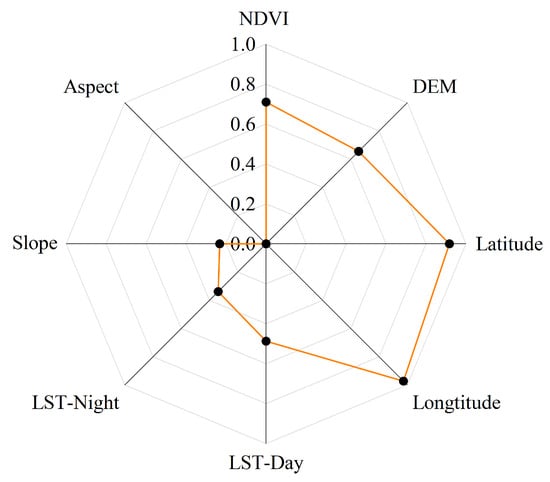
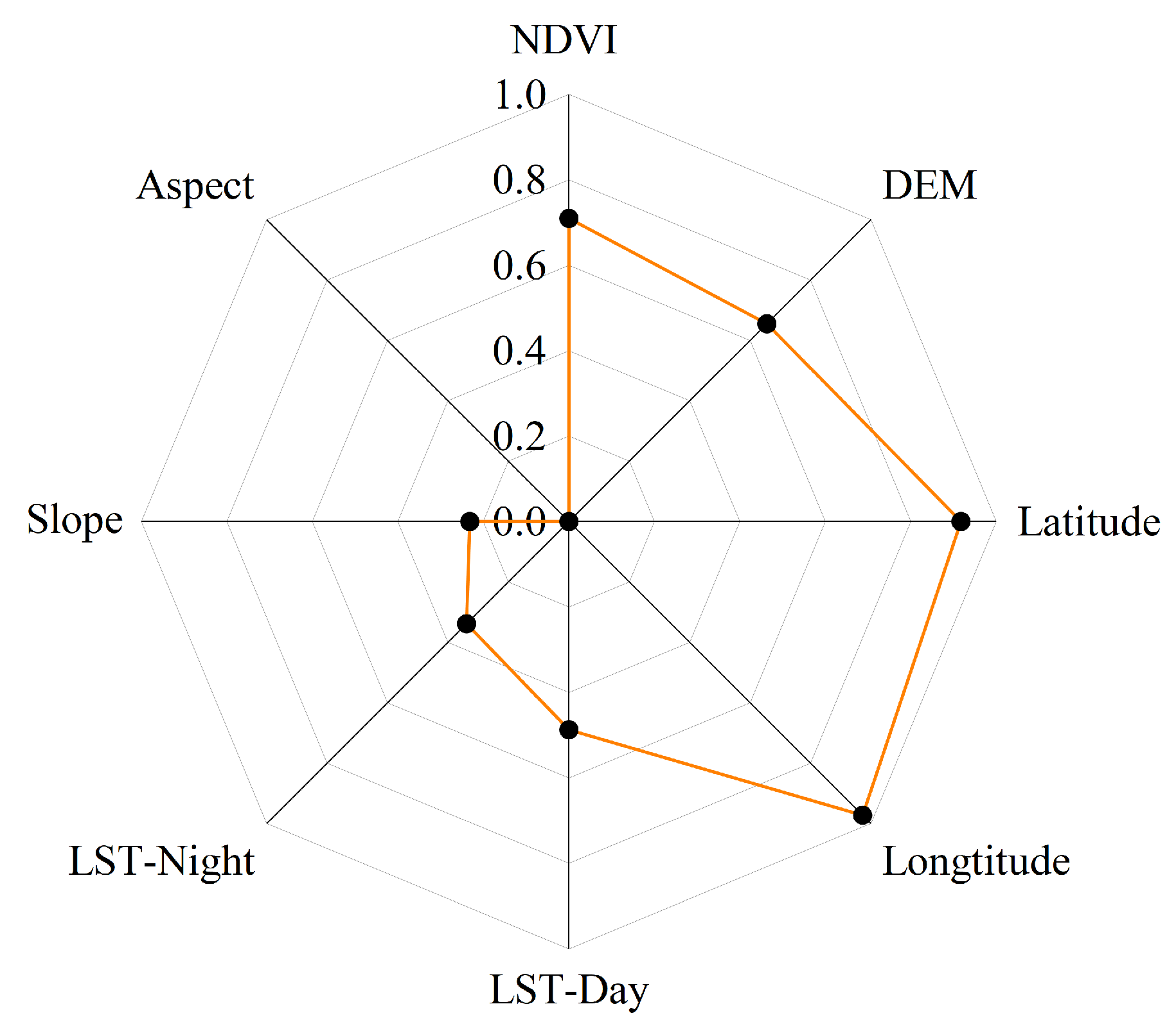
When constructing the machine learning models, the importance of each environmental variable was calculated based on its contribution to the regression model. Figure 8 shows the importance of the environmental variables in building the regression model based on the Cubist model, with values ranging from 0 to 1.
Figure 8.
Comparison of the importance of environmental variables. Black dots indicate the normalized importance value of each variable, and the yellow line connects these points to form a polygon for visual comparison of relative importance.
Longitude and latitude have the highest importance in the regression model, indicating that their effects are significant in downscaling TRMM data for the Qaidam Basin. The spatial distribution of precipitation in the Qaidam Basin showed a gradually decreasing trend from the eastern and southern parts toward the northwestern interior. The NDVI and elevation were second only to longitude and latitude in importance, highlighting the NDVI’s significant contribution to model construction. The influence of precipitation on vegetation has been widely recognized [43,44,45]. The contribution of the DEM was not significantly different from that of the NDVI; precipitation in the Qaidam Basin increases with elevation, and precipitation is closely related to the NDVI and DEM [46]. LST-day and LST-night also contributed to a certain extent. Precipitation moistens the land surface, and energy is then used more for evaporation rather than sensible heat transport. After rainfall, bare soil exhibits higher evaporation intensity [19,47]. The Qaidam Basin is an arid inland basin, especially within the basin interior, where vegetation is sparse, making the effect of precipitation on LST more pronounced. Among all the environmental variables, slope and aspect exhibited the weakest contributions.
5.3. Limitations of the Study
The Qaidam Basin is a high-altitude, cold, and arid inland basin where vegetation growth in most areas depends on precipitation. Therefore, this study assumes a positive correlation between precipitation and the NDVI when establishing the model. However, the relationship between precipitation and the NDVI is susceptible to various natural and anthropogenic factors, constraining the development of downscaled models. In terms of natural factors, the Qaidam Basin contains rivers, lakes, and groundwater discharge, and pixels covered by water bodies have NDVI values below 0. Because of replenishment from these water bodies, vegetation growth is better than in other areas. However, vegetation growth has little relationship with precipitation. In terms of human factors, agricultural activities altered the spatial distribution pattern of the NDVI and its temporal variation trends in the plains of the Qaidam Basin. In this study, pixels with NDVI values below 0 were removed during data preprocessing. Low-pass filtering was used to exclude anomalous NDVI regions. However, the window size used for low-pass filtering determines the extent to which anomalous NDVI regions are removed, introducing uncertainty. Jia et al. [21] used Moran’s I to remove anomalous pixels unrelated to precipitation. However, some weakly correlated pixels were retained in their study [48]. Therefore, it is necessary to further investigate the methods for removing NDVI anomalies.
To further improve the accuracy of downscaled data, previous studies have used a portion of in situ station precipitation observations to correct the downscaling results. Two correction methods have been commonly adopted: the Geographic Difference Analysis (GDA) method and the Geographic Ratio Analysis (GRA) method [16]. The remaining station precipitation data were then used to validate the corrected precipitation data, and the results showed that downscaled data quality improves after correction [2,49,50]. However, the Qaidam Basin is a data-scarce region. With a total area of approximately 275,000 km2, it has only nine meteorological stations. Although this study delineated a buffer zone, there are still only 17 meteorological stations even with the buffer, and the station distribution remains very sparse. This limits effective correction of precipitation data, thereby affecting precipitation accuracy, and constitutes a key challenge for downscaling research in all data-scarce regions. Therefore, to further enhance downscaling performance in data-scarce regions, future studies should use the limited station data to apply bias correction to the original TRMM data either before or after downscaling, because biases inherent in the TRMM data itself may affect the accuracy of the downscaling results.
6. Conclusions
In this study, we focused on the Qaidam Basin as the study area and selected longitude, latitude, the NDVI, the DEM, daytime and nighttime LST, slope, and aspect as the environmental variables. Using TRMM data from 2000 to 2019, a downscaling analysis was conducted based on four methods—ANN, Cubist, Random Forest (RF), and Support Vector Machines (SVM)—and validated using observations from ground meteorological stations. The annual downscaled data were then disaggregated into monthly precipitation data using the proportional coefficient method, and the accuracy was further assessed. The main conclusions are as follows.
- (1)
- The validation results demonstrated that for both annual and monthly downscaled data, the Cubist-based model achieved the highest accuracy among the four machine learning methods, followed by the ANN model. Meanwhile, the RF and SVM models yielded the lowest accuracy. The residual correction improved the precision of the data.
- (2)
- The spatial distribution results indicate that the annual downscaling outputs based on the four machine learning methods exhibit spatial patterns similar to the original TRMM data, with precipitation decreasing from the southeast to the northwest. They also eliminate the outliers present in the original TRMM data. The downscaled data produced by the ANN, Cubist, and RF models show relatively smooth spatial distributions. Meanwhile, the SVM-based downscaled data display a more fragmented pattern. The downscaled results provide a fine-grained spatial pattern for the spatial distribution of the monthly downscaled data.
- (3)
- Among the environmental variables, longitude and latitude were the most important, followed by the DEM and NDVI. Daytime and nighttime LST also contributed to some extent, whereas slope and aspect had the lowest contribution rates.
Qaidam Basin is a data-scarce region. By developing regression models between precipitation and environmental variables, we downscaled satellite precipitation data to provide precipitation datasets with higher spatiotemporal resolution for the Qaidam Basin. This is of considerable importance for gaining an in-depth understanding of the water cycle in high-altitude arid basins.
Author Contributions
Conceptualization, Y.W. and C.Y.; methodology, Y.W. and X.J.; software, Y.W. and Q.M.; validation, Y.W., C.Y., X.J. and Q.M.; formal analysis, Y.W. and Q.M.; investigation, C.Y. and X.J.; resources, X.J.; data curation, Y.W. and Q.M.; writing—original draft preparation, Y.W.; writing—review and editing, Y.W. and X.J.; visualization, Y.W.; supervision, C.Y., X.J. and Q.M.; project administration, X.J.; funding acquisition, X.J. All authors have read and agreed to the published version of the manuscript.
Funding
This research was funded by the Research and Innovation Team Project for Safety Guarantee of Major Projects in Sandy Areas (E455020601), National Key R&D Program (2018YFC0406600) and Key Deployment Project of Chinese Academy of Sciences (ZDRW-ZS-2019-3, ZDRW-ZS-2020-3).
Data Availability Statement
The data presented in this study are available on request from the first author.
Acknowledgments
The authors would like to thank NASA for providing the MODIS, TRMM, and DEM data used in this study. Thanks to the China Meteorological Data Service Centre for providing the rain gauge data. We also thank the teachers and students of the State Key Laboratory of Ecological Safety and Sustainable Development in Arid Lands for their support. In addition, we thank the editors and reviewers for their insightful and valuable comments.
Conflicts of Interest
The authors declare no conflicts of interest.
Abbreviations
The following abbreviations are used in this manuscript:
| TRMM | Tropical Rainfall Measuring Mission |
| ANN | Artificial Neural Network |
| RF | Random Forest |
| SVR | Support Vector Machine |
| NDVI | Normalized Difference Vegetation Index |
| LST | Land Surface Temperature |
| DEM | Digital Elevation Model |
References
- Liu, C.; Wang, Z.; Yang, S.; Sang, Y.; Liu, X.; Li, J. Hydro-Informatic Modeling System: Aiming at water cycle in land surface material and energy exchange processes. Acta Geogr. Sin. 2014, 69, 579–587. [Google Scholar]
- Noor, R.; Arshad, A.; Shafeeque, M.; Liu, J.; Baig, A.; Ali, S.; Maqsood, A.; Pham, Q.B.; Dilawar, A.; Khan, S.N. Combining APHRODITE rain gauges-based precipitation with downscaled-TRMM data to translate high-resolution precipitation estimates in the indus basin. Remote Sens. 2023, 15, 318. [Google Scholar] [CrossRef] [Scilit]
- Ceccherini, G.; Ameztoy, I.; Romero Hernández, C.P.; Carmona Moreno, C. High-resolution precipitation datasets in South America and West Africa based on satellite-derived rainfall, enhanced vegetation index and digital elevation model. Remote Sens. 2015, 7, 6454–6488. [Google Scholar] [CrossRef] [Scilit]
- Xu, S.; Wu, C.; Wang, L.; Gonsamo, A.; Shen, Y.; Niu, Z. A new satellite-based monthly precipitation downscaling algorithm with non-stationary relationship between precipitation and land surface characteristics. Remote Sens. Environ. 2015, 162, 119–140. [Google Scholar] [CrossRef] [Scilit]
- Kyriakidis, P.C.; Kim, J.; Miller, N.L. Geostatistical mapping of precipitation from rain gauge data using atmospheric and terrain characteristics. J. Appl. Meteorol. Climatol. 2001, 40, 1855–1877. [Google Scholar] [CrossRef] [Scilit]
- Nastos, P.; Kapsomenakis, J.; Philandras, K. Evaluation of the TRMM 3B43 gridded precipitation estimates over Greece. Atmos. Res. 2016, 169, 497–514. [Google Scholar] [CrossRef] [Scilit]
- Michaelides, S.; Levizzani, V.; Anagnostou, E.; Bauer, P.; Kasparis, T.; Lane, J. Precipitation: Measurement, remote sensing, climatology and modeling. Atmos. Res. 2009, 94, 512–533. [Google Scholar] [CrossRef] [Scilit]
- Jiang, S.; Ren, L.; Hong, Y.; Yong, B.; Yang, X.; Yuan, F.; Ma, M. Comprehensive evaluation of multi-satellite precipitation products with a dense rain gauge network and optimally merging their simulated hydrological flows using the Bayesian model averaging method. J. Hydrol. 2012, 452, 213–225. [Google Scholar] [CrossRef] [Scilit]
- Gebremichael, M.; Anagnostou, E.N.; Bitew, M.M. Critical steps for continuing advancement of satellite rainfall applications for surface hydrology in the Nile River basin 1. JAWRA J. Am. Water Resour. Assoc. 2010, 46, 361–366. [Google Scholar] [CrossRef] [Scilit]
- Kummerow, C.; Barnes, W.; Kozu, T.; Shiue, J.; Simpson, J. The tropical rainfall measuring mission (TRMM) sensor package. J. Atmos. Ocean. Technol. 1998, 15, 809–817. [Google Scholar] [CrossRef] [Scilit]
- Prakash, S.; Mitra, A.K.; AghaKouchak, A.; Liu, Z.; Norouzi, H.; Pai, D. A preliminary assessment of GPM-based multi-satellite precipitation estimates over a monsoon dominated region. J. Hydrol. 2018, 556, 865–876. [Google Scholar] [CrossRef] [Scilit]
- Joyce, R.J.; Janowiak, J.E.; Arkin, P.A.; Xie, P. CMORPH: A method that produces global precipitation estimates from passive microwave and infrared data at high spatial and temporal resolution. J. Hydrometeorol. 2004, 5, 487–503. [Google Scholar] [CrossRef] [Scilit]
- Kubota, T.; Shige, S.; Hashizume, H.; Aonashi, K.; Takahashi, N.; Seto, S.; Hirose, M.; Takayabu, Y.N.; Ushio, T.; Nakagawa, K. Global precipitation map using satellite-borne microwave radiometers by the GSMaP project: Production and validation. IEEE Trans. Geosci. Remote Sens. 2007, 45, 2259–2275. [Google Scholar] [CrossRef] [Scilit]
- Wang, Q.; Jin, X. Accuracy Evaluation of the TRMM and GPM Precipitation Data in Qaidam Basin. Yellow River 2022, 44, 16–20. [Google Scholar]
- Li, Y. Spatial Downscaling Study of Three Remotely Sensed Precipitation Products in Qinghai Lake Basin and Analysis of Temporal and Spatial Changes. Master’s Thesis, Qinghai Normal University, Xining, China, 2023. [Google Scholar]
- Duan, Z.; Bastiaanssen, W. First results from Version 7 TRMM 3B43 precipitation product in combination with a new downscaling–calibration procedure. Remote Sens. Environ. 2013, 131, 1–13. [Google Scholar] [CrossRef] [Scilit]
- Park, N.-W. Spatial downscaling of TRMM precipitation using geostatistics and fine scale environmental variables. Adv. Meteorol. 2013, 2013, 237126. [Google Scholar] [CrossRef] [Scilit]
- Immerzeel, W.; Rutten, M.; Droogers, P. Spatial downscaling of TRMM precipitation using vegetative response on the Iberian Peninsula. Remote Sens. Environ. 2009, 113, 362–370. [Google Scholar] [CrossRef] [Scilit]
- De Kauwe, M.G.; Taylor, C.M.; Harris, P.P.; Weedon, G.P.; Ellis, R.J. Quantifying land surface temperature variability for two Sahelian mesoscale regions during the wet season. J. Hydrometeorol. 2013, 14, 1605–1619. [Google Scholar] [CrossRef] [Scilit]
- Trenberth, K.E.; Shea, D.J. Relationships between precipitation and surface temperature. Geophys. Res. Lett. 2005, 32, L14703. [Google Scholar] [CrossRef] [Scilit]
- Jia, S.; Zhu, W.; Lű, A.; Yan, T. A statistical spatial downscaling algorithm of TRMM precipitation based on NDVI and DEM in the Qaidam Basin of China. Remote Sens. Environ. 2011, 115, 3069–3079. [Google Scholar] [CrossRef] [Scilit]
- Foody, G. Geographical weighting as a further refinement to regression modelling: An example focused on the NDVI–rainfall relationship. Remote Sens. Environ. 2003, 88, 283–293. [Google Scholar] [CrossRef] [Scilit]
- Jing, W.; Yang, Y.; Yue, X.; Zhao, X. A spatial downscaling algorithm for satellite-based precipitation over the Tibetan plateau based on NDVI, DEM, and land surface temperature. Remote Sens. 2016, 8, 655. [Google Scholar] [CrossRef] [Scilit]
- Elnashar, A.; Zeng, H.; Wu, B.; Zhang, N.; Tian, F.; Zhang, M.; Zhu, W.; Yan, N.; Chen, Z.; Sun, Z. Downscaling TRMM monthly precipitation using google earth engine and google cloud computing. Remote Sens. 2020, 12, 3860. [Google Scholar] [CrossRef] [Scilit]
- Ma, Z.; Shi, Z.; Zhou, Y.; Xu, J.; Yu, W.; Yang, Y. A spatial data mining algorithm for downscaling TMPA 3B43 V7 data over the Qinghai–Tibet Plateau with the effects of systematic anomalies removed. Remote Sens. Environ. 2017, 200, 378–395. [Google Scholar] [CrossRef] [Scilit]
- Han, T.; Qi, D.; Chen, H.; Xiang, S.; Shi, X.; Liu, C.; Li, N.; Wu, S. Spatial and Temporal Distribution of Precipitation in Qaidam Basin. Desert Oasis Meteorol. 2019, 13, 69–75. [Google Scholar]
- Liu, Y. Rational Utilization of Water Resources and Ecological Environment Protection of Qaidam Basin, 1st ed.; Science Press: Beijing, China, 2000; pp. 1–20. [Google Scholar]
- Lv, A.; Zhou, L. A rainfall model based on a geographically weighted regression algorithm for rainfall estimations over the arid Qaidam Basin in China. Remote Sens. 2016, 8, 311. [Google Scholar] [CrossRef] [Scilit]
- Zhu, W.; Lv, A.; Jia, S. Study on spatial distribution of vegetation coverage and its affecting factors in the Qaidam Basin based on NDVI. Arid. Zone Res 2010, 27, 691–698. [Google Scholar]
- Huffman, G.J.; Bolvin, D.T.; Nelkin, E.J.; Wolff, D.B.; Adler, R.F.; Gu, G.; Hong, Y.; Bowman, K.P.; Stocker, E.F. The TRMM multisatellite precipitation analysis (TMPA): Quasi-global, multiyear, combined-sensor precipitation estimates at fine scales. J. Hydrometeorol. 2007, 8, 38–55. [Google Scholar] [CrossRef] [Scilit]
- Warren, S.D.; Hohmann, M.G.; Auerswald, K.; Mitasova, H. An evaluation of methods to determine slope using digital elevation data. CATENA 2004, 58, 215–233. [Google Scholar] [CrossRef] [Scilit]
- Chen, J.; Jönsson, P.; Tamura, M.; Gu, Z.; Matsushita, B.; Eklundh, L. A simple method for reconstructing a high-quality NDVI time-series data set based on the Savitzky–Golay filter. Remote Sens. Environ. 2004, 91, 332–344. [Google Scholar] [CrossRef] [Scilit]
- Were, K.; Bui, D.T.; Dick, Ø.B.; Singh, B.R. A comparative assessment of support vector regression, artificial neural networks, and random forests for predicting and mapping soil organic carbon stocks across an Afromontane landscape. Ecol. Indic. 2015, 52, 394–403. [Google Scholar] [CrossRef] [Scilit]
- Quinlan, J.R. Improved use of continuous attributes in C4. 5. J. Artif. Intell. Res. 1996, 4, 77–90. [Google Scholar] [CrossRef] [Scilit]
- Breiman, L. Random forests. Mach. Learn. 2001, 45, 5–32. [Google Scholar] [CrossRef] [Scilit]
- Cortes, C. Support-Vector Networks. Mach. Learn. 1995, 20, 273–297. [Google Scholar] [CrossRef] [Scilit]
- Jing, W.; Yang, Y.; Yue, X.; Zhao, X. A comparison of different regression algorithms for downscaling monthly satellite-based precipitation over North China. Remote Sens. 2016, 8, 835. [Google Scholar] [CrossRef] [Scilit]
- Pedregosa, F.; Varoquaux, G.; Gramfort, A.; Michel, V.; Thirion, B.; Grisel, O.; Blondel, M.; Prettenhofer, P.; Weiss, R.; Dubourg, V. Scikit-learn: Machine learning in Python. J. Mach. Learn. Res. 2011, 12, 2825–2830. [Google Scholar]
- Zeng, N.; Ren, X.; He, H.; Zhang, L.; Li, P.; Niu, Z. Estimating the grassland aboveground biomass in the Three-River Headwater Region of China using machine learning and Bayesian model averaging. Environ. Res. Lett. 2021, 16, 114020. [Google Scholar] [CrossRef] [Scilit]
- Yin, Z.; Zhang, X.; Liu, X.; Colella, M.; Chen, X. An assessment of the biases of satellite rainfall estimates over the Tibetan Plateau and correction methods based on topographic analysis. J. Hydrometeorol. 2008, 9, 301–326. [Google Scholar] [CrossRef] [Scilit]
- Tang, G.; Long, D.; Hong, Y. Systematic anomalies over inland water bodies of High Mountain Asia in TRMM precipitation estimates: No longer a problem for the GPM era? IEEE Geosci. Remote Sens. Lett. 2016, 13, 1762–1766. [Google Scholar] [CrossRef] [Scilit]
- Guanghua, X.; Xianli, X.; Meixian, L.; Alexander, S.; Kelin, W. Spatial Downscaling of TRMM Precipitation Product Using a Combined Multifractal and Regression Approach: Demonstration for South China. Water 2015, 7, 3083–3102. [Google Scholar] [CrossRef] [Scilit]
- Zhang, Y.; Li, Y.; Ji, X.; Luo, X.; Li, X. Fine-resolution precipitation mapping in a mountainous watershed: Geostatistical downscaling of TRMM products based on environmental variables. Remote Sens. 2018, 10, 119. [Google Scholar] [CrossRef] [Scilit]
- Zhang, X.; Friedl, M.A.; Schaaf, C.B.; Strahler, A.H.; Liu, Z. Monitoring the response of vegetation phenology to precipitation in Africa by coupling MODIS and TRMM instruments. J. Geophys. Res. Atmos. 2005, 110, D12103. [Google Scholar] [CrossRef] [Scilit]
- Jaber, S.M. Comparative evaluation of statistically downscaling Tropical Rainfall Measuring Mission (TRMM) and Global Precipitation Measurement (GPM) mission precipitation data: Evidence from a typical semi-arid to arid environment. Spat. Inf. Res. 2021, 29, 331–338. [Google Scholar] [CrossRef] [Scilit]
- Arshad, A.; Mirchi, A.; Samimi, M.; Ahmad, B. Combining downscaled-GRACE data with SWAT to improve the estimation of groundwater storage and depletion variations in the Irrigated Indus Basin (IIB). Sci. Total Environ. 2022, 838, 156044. [Google Scholar] [CrossRef] [Scilit] [PubMed]
- Wallace, J.; Holwill, C. Soil evaporation from tiger-bush in south-west Niger. J. Hydrol. 1997, 188, 426–442. [Google Scholar] [CrossRef] [Scilit]
- Duan, L.; Fan, K.; Li, W.; Liu, T. Spatial downscaling algorithm of TRMM precipitation based on multiple high-resolution satellite data for Inner Mongolia, China. Theor. Appl. Climatol. 2019, 135, 45–59. [Google Scholar] [CrossRef] [Scilit]
- Zhang, H.; Wei, M.; Qin, J.; Xu, Y.; Dou, S. Downscaling and Error Correction of TRMM Data Based on Different Vegetation Indices. Bull. Soil Water Conserv. 2021, 41, 214–223. [Google Scholar]
- Arshad, A.; Zhang, W.; Zhang, Z.; Wang, S.; Zhang, B.; Cheema, M.J.M.; Shalamzari, M.J. Reconstructing high-resolution gridded precipitation data using an improved downscaling approach over the high altitude mountain regions of Upper Indus Basin (UIB). Sci. Total Environ. 2021, 784, 147140. [Google Scholar] [CrossRef] [Scilit]

Disclaimer/Publisher’s Note: The statements, opinions and data contained in all publications are solely those of the individual author(s) and contributor(s) and not of MDPI and/or the editor(s). MDPI and/or the editor(s) disclaim responsibility for any injury to people or property resulting from any ideas, methods, instructions or products referred to in the content. |
© 2026 by the authors. Licensee MDPI, Basel, Switzerland. This article is an open access article distributed under the terms and conditions of the Creative Commons Attribution (CC BY) license.