Machine-Learning-Based Historical Reconstruction of Soil Organic Carbon Dynamics in Coastal Tidal Flats: Quantifying the Spatiotemporal Impacts of Reclamation

Highlights

What are the main findings?

• Reclamation reduced tidal flat area by 61.92%, and SOC in the remaining tidal flats declined by 18.98%.
• Conversion to farmlands shows the greatest potential for carbon sequestration in reclaimed areas.

What are the implications of the main findings?

• Machine learning reconstructs soil organic carbon dynamics in coastal tidal flats from 2000 to 2020.
• Reclamation impacts on SOC exhibit pronounced cumulative effects and time-lagged responses.

Abstract

Coastal tidal flat soil organic carbon (SOC) is significantly affected by reclamation activities. However, the limited availability of historical SOC data constrains the reconstruction of past SOC. SOC data were integrated in current time-point and remote sensing data during the last two decades by applying machine learning (ML) methods such as random forest (RF), boosted regression trees (BRT), and extreme gradient boosting (XGBoost) to map the spatiotemporal distribution of tidal flat reclamation and the spatial distribution of SOC content in the western coastal region of the Bohai Rim over the last two decades and to explore how the period and type of reclamation affect SOC content. The results show that: (1) The area of tidal flats decreased by 61.92% from 2000 to 2020 due to reclamation activities. (2) Among the ML methods, the XGBoost model demonstrated the best performance (R² = 0.71, MAE = 0.93 g/kg, RMSE = 1.32 g/kg, d-Willmott = 0.98), with the modified normalized difference water index (MNDWI) being the most important predictor variable. (3) The SOC content of tidal flats decreased from 4.11 g/kg in 2000 to 3.33 g/kg in 2020, a reduction of 18.98%. (4) The reclamation of tidal flats into marshes, forest lands, grasslands, farmlands, and bare lands led to an increasing trend in SOC content, with the greatest increase observed in regions converted to farmlands. This study provides data support for the control of reclamation activities, creation of tidal flat conservation policies, and strategic decision-making for climate change mitigation.

1. Introduction

Soil organic carbon (SOC) is a central hub of the global carbon cycle [1]. Tidal flat SOC pools are vulnerable to human actions and represent a distinct category among the ecosystem organic carbon pools [2]. Since the 21st century, economic and demographic expansion, along with urbanization, has led to an increased demand for space [3]. Tidal flats have become prime targets for development and have undergone long-term and large-scale reclamation, which has significantly impacted the soil carbon balance of these regions [4,5,6]. Therefore, examining the effects of tidal flat reclamation on SOC is crucial for controlling reclamation activities, developing tidal flat conservation plans, and informing strategic choices to mitigate climate change.

The effects of tidal flat reclamation on SOC exhibit significant variability and uncertainty. In Dongtai, Jiangsu Province, SOC content decreases as the number of reclamation years increases [7]. However, SOC significantly increased within 30 years after reclamation, especially in areas converted to farmlands in Rudong [8]. Despite the geographical proximity of the two study areas, the impacts of reclamation on SOC show distinct trends. Moreover, different types of reclamation exert significantly different impacts on SOC content [9]. The period and type of reclamation have a major impact on SOC, but the mechanisms behind these effects remain unclear. Therefore, it is crucial to comprehend the influence of tidal flat reclamation on SOC.

Traditional SOC measurements based on field samples are accurate but are time-consuming, labor-intensive, and destructive [10]. Moreover, the low accessibility of tidal flat regions poses a significant challenge for large-scale sampling [11]. Remote sensing technology offers abundant multi-source data, facilitating the extraction of numerous features and providing crucial data support for digital soil mapping (DSM) [12]. Current DSM still primarily relies on reflectance features and remote sensing indices [13]. However, besides spectral features, environmental factors often influence SOC content [14]. Integrating these environmental factors can enhance the spatial prediction accuracy of SOC [15]. Therefore, how to fully utilize remote sensing data in combination with environmental factors to predict SOC content and analyze its dynamic variations remains an urgent issue requiring further in-depth investigation.

To predict SOC content, researchers applied several statistical models, including geostatistical models, linear models, and machine learning (ML) models [16], while geostatistical and linear models may depict the linear relationship between variables and independent variables [14]. Nevertheless, predominantly nonlinear relationships exist between soil physicochemical properties and predictor variables [15]. Tree-based models such as Random Forest (RF), Boosted Regression Tree (BRT), and Extreme Gradient Boosting (XGBoost) excel at capturing and identifying nonlinear relationships. They offer enhanced reliability and robustness, showing great potential for the prediction of SOC content [17].

Accurately predicting SOC content and analyzing its spatial distribution patterns, as well as achieving spatiotemporal simulation of SOC content from “point to region” and from “present to past,” has become a key research topic [18]. Based on Landsat imagery, a study analyzed the spatiotemporal distribution of SOC content in the Yancheng coastal wetlands from 2000 to 2022 [19]. The results indicate that from 2000 to 2022, both SOC stock and SOC density gradually increased, reaching a peak in 2016. Another study combined field soil data from the current year with remote sensing data from 1988 to 2020 to estimate the SOC stock on Chongming Island [20]. The findings reveal that from 1988 to 2020, the surface SOC stock on the whole island exhibited an overall increasing trend. In arid regions of Iran, researchers constructed a model based on SOC data from 2016 and Landsat remote sensing data, and then retrospectively applied this model to 1986, 1999, and 2010 to reconstruct the spatiotemporal dynamics of SOC over the past 30 years [21]. The results indicate that SOC in the study area exhibits a significant overall declining trend. These studies clearly demonstrate that even in the absence of historical soil data, it is feasible to construct models utilizing current-year data and perform spatial reconstruction of SOC content for historical periods. This provides a novel technique for the spatiotemporal dynamic analysis of SOC content.

This study employs time-series remote sensing image data from the western coastal region of the Bohai Rim to extract spatial distribution information on tidal flat reclamation across different years. By integrating field SOC data in current time point and remote sensing data during the last two decades, three ML models were used to reconstruct the spatiotemporal distribution of SOC content in coastal tidal flats, enabling “from present to past” SOC mapping and quantitatively analyzing SOC changes induced by tidal flat reclamation activities. The study objectives include: (1) to investigate the spatiotemporal variation features of tidal flat reclamation; (2) evaluate the performance of SOC content prediction models and interpret the constructed models using relative importance analysis; and (3) to comprehensively analyze the combined effects of reclamation period and type on the spatiotemporal evolution of SOC content and to conduct a quantitative assessment. The main purpose of this study is to provide a feasible method to investigate the spatiotemporal characteristics of SOC changes induced by tidal flat reclamation in the premise of absence of historical SOC data.

2. Materials and Methods

This study took both the reclamation period and type into account to conduct a quantitative analysis of the impact of tidal flat reclamation on SOC content. We utilized Landsat images and employed a hybrid approach that employed object-oriented and decision-tree methods to create land cover maps for the western coastal region of the Bohai Rim. This made it possible to extract spatial distribution information on tidal flat reclamation across different periods. Then, using multi-source data along with observed soil data, we constructed SOC content prediction models employing RF, BRT, and XGBoost, and determined the optimal model by comparative analysis. Next, using a temporal transfer approach of the model, we performed a current estimate (2020) and historical reconstruction and inversion (2000–2015) of SOC content. Finally, based on the two aforementioned components, we analyzed the influence of tidal flat reclamation on SOC content.

2.1. Study Area

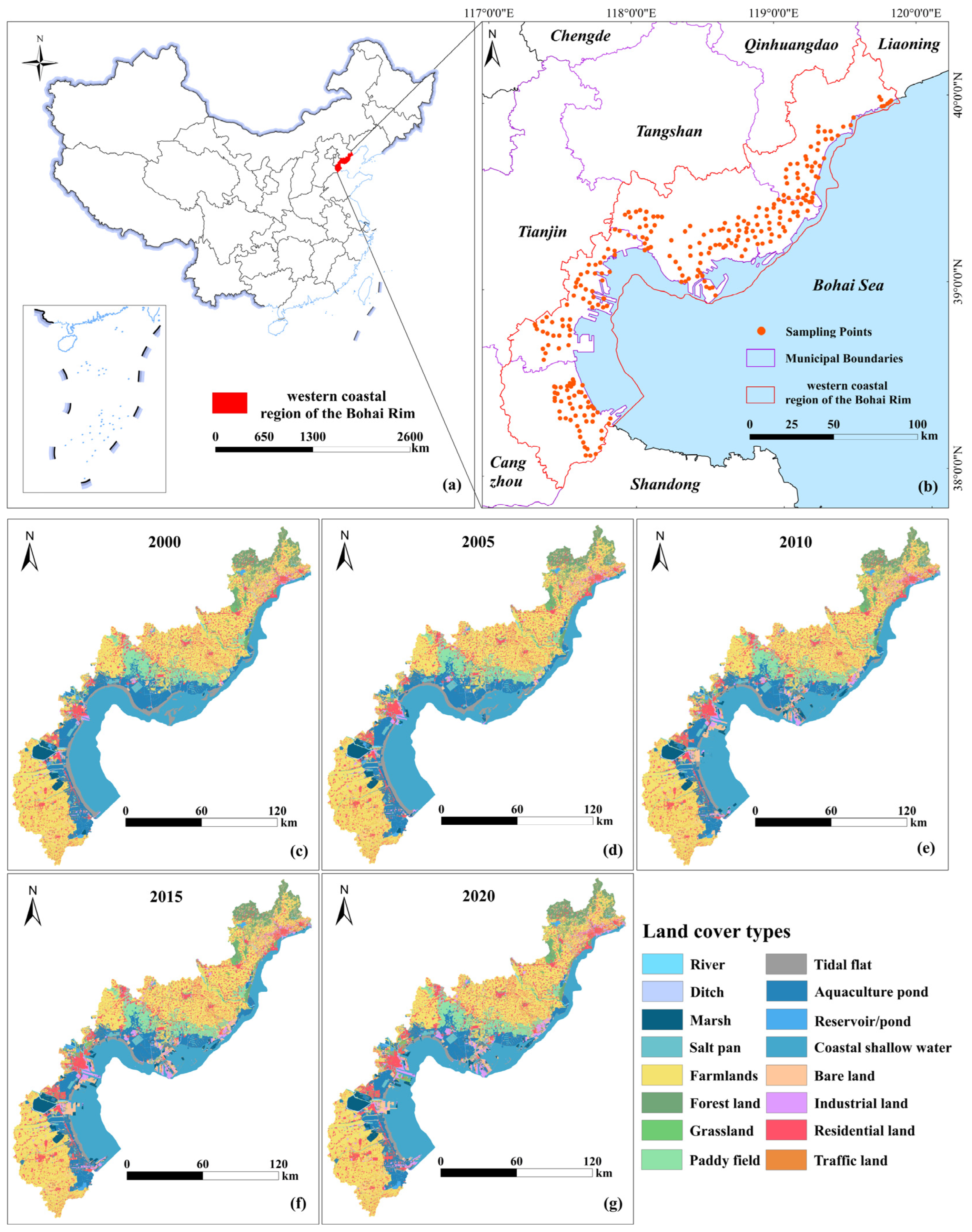
The western coastal region of the Bohai Rim (ranges from 117°25′ to 119°53′E and from 38°07′ to 40°05′N) encompasses the coastal regions of Qinhuangdao, Tangshan, Tianjin, and Cangzhou. It serves as a crucial distribution area for coastal wetlands in China. On the landward side, the administrative boundaries of 12 coastal counties and districts delineate the terrestrial border. The seaward boundary is determined by the −6 m isobath, which marks the outer limit of the coastal wetlands. The study area spans approximately 17,633.58 km² and has a total coastline length of approximately 640.20 km (Figure 1a,b).

2.2. Data Collection

2.2.1. Soil Sampling and Analysis

Soil samples were collected annually from July to October during 2019–2021. Taking into account the size of the study area and the spatial distribution characteristics of the intertidal zone, and with reference to the relevant requirements of the Technical Specification for Soil Environmental Monitoring, the straight-line distance between sampling sites was set to approximately 5 km to meet the requirements for spatial representativeness and monitoring density in soil sampling. During the soil sample collection process, the predefined sampling points were adjusted as necessary based on actual field conditions to ensure the accuracy of the soil samples. Surface soil samples (0–30 cm) were collected when the surface water level was relatively low, collecting a total of 265 valid samples (Figure 1b). At each sampling point, three soil profiles were collected to create a composite sample, which was then air-dried, crushed, and sieved [22]. The SOC content was observed using a Shimadzu total organic carbon analyzer (Shimadzu Corporation, Kyoto, Japan) [23].

Descriptive statistical analysis was performed on the SOC content across different coastal regions (

Table 1. SOC content descriptive statistics of soil samples.

Coastal Region	Number	Minimum (g/kg)	Maximum (g/kg)	Mean (g/kg)	SD (g/kg)	CV (%)
Qinhuangdao	51	0.26	25.72	7.51	6.28	83.64
Tangshan	106	0.46	15.73	6.97	3.62	51.88
Tianjin	56	1.36	30.74	8.34	5.75	68.97
Cangzhou	52	1.76	18.69	6.67	3.44	51.51

Notes: SD, standard deviation; CV, coefficient of variation.

). The analysis indicated that the average SOC content is highest in the Tianjin coastal region at 8.34 g/kg and lowest in the Cangzhou coastal region at 6.67 g/kg. All coastal regions exhibit moderate levels of variability [24].

2.2.2. Acquisition and Processing of Remote Sensing Imagery

The remote sensing imagery data were acquired from the United States Geological Survey website (http://glovis.usgs.gov/, accessed on 30 July 2024). Five periods of Landsat remote sensing images were selected using 5-year intervals from 2000 to 2020. To extract remote sensing features corresponding to the soil samples and ensure image quality, Landsat images acquired during the low-tide period from July to October were selected, and cloud cover was maintained below 5.00%. During this period, vegetation cover was relatively high, which facilitated the extraction of spectral features for identifying the spatial distribution of land-use types in the study area and for calculating remote sensing indices. Among them, the 2020 image was mosaicked from images of the corresponding sampling areas for each year from 2019 to 2021. Remote sensing imagery from each time point year was used for land-cover classification and for extracting predictor variables for the corresponding year.

Based on the pre-processed remote sensing imagery, band reflectance, remote sensing indices, and texture features were extracted. Band reflectance includes the red band (B_Red), green band (B_Green), blue band (B_Blue), near infrared band (B_NIR), shortwave infrared band I (B_SWIR1), and shortwave infrared band II (B_SWIR2) from the Landsat remote sensing images. By performing mathematical operations on the relevant bands of the Landsat images, indices such as normalized difference vegetation index (NDVI), difference vegetation index (DVI), ratio vegetation index (RVI), kernel normalized difference vegetation index (KNDVI), and modified normalized difference water index (MNDWI) were constructed to build the model factor database (

Table 2. Definitions and calculation formulas of vegetation indices.

Vegetation Indices	Calculation Formula	Literature
Chlorophyll vegetation index (CVI)	$\left({\mathrm{B}}_{\mathrm{NIR}}/{\mathrm{B}}_{\mathrm{Green}}\right)\times \left({\mathrm{B}}_{\mathrm{Red}}/{\mathrm{B}}_{\mathrm{Green}}\right)$	[27]
Difference vegetation index (DVI)	$2.4\times {\mathrm{B}}_{\mathrm{NIR}}-{\mathrm{B}}_{\mathrm{Red}}$	[28]
Enhanced vegetation index (EVI)	$2.5\left({\mathrm{B}}_{\mathrm{NIR}}-{\mathrm{B}}_{\mathrm{Red}}\right)/\left({\mathrm{B}}_{\mathrm{NIR}}+6\times {\mathrm{B}}_{\mathrm{Red}}-7.5\times {\mathrm{B}}_{\mathrm{Blue}}+1\right)$	[29]
Ratio vegetation index (RVI)	${\mathrm{B}}_{\mathrm{Red}}/{\mathrm{B}}_{\mathrm{NIR}}$	[30]
Normalized difference index (NDI)	$\left({\mathrm{B}}_{\mathrm{NIR}}-{\mathrm{B}}_{\mathrm{SWIR}1}\right)/\left({\mathrm{B}}_{\mathrm{NIR}}+{\mathrm{B}}_{\mathrm{SWIR}1}\right)$	[31]
Water ratio index (WRI)	$\left({\mathrm{B}}_{\mathrm{Green}}+{\mathrm{B}}_{\mathrm{Red}}\right)/\left({\mathrm{B}}_{\mathrm{NIR}}+{\mathrm{B}}_{\mathrm{SWIR}1}\right)$	[32]
Normalized difference vegetation index (NDVI)	$\left({\mathrm{B}}_{\mathrm{NIR}}-{\mathrm{B}}_{\mathrm{Red}}\right)/\left({\mathrm{B}}_{\mathrm{NIR}}+{\mathrm{B}}_{\mathrm{Red}}\right)$	[33]
Normalized difference soil index (NDSI)	$\left({\mathrm{B}}_{\mathrm{SWIR}1}-{\mathrm{B}}_{\mathrm{SWIR}2}\right)/\left({\mathrm{B}}_{\mathrm{SWIR}1}+{\mathrm{B}}_{\mathrm{SWIR}2}\right)$	[34]
Normalized difference water index (NDWI)	$\left({\mathrm{B}}_{\mathrm{Green}}-{\mathrm{B}}_{\mathrm{NIR}}\right)/\left({\mathrm{B}}_{\mathrm{Green}}+{\mathrm{B}}_{\mathrm{NIR}}\right)$	[35]
Renormalized difference vegetation index (RDVI)	$\sqrt{\mathrm{NDVI}\times \mathrm{DVI}}$	[36]
Soil adjusted vegetation index (SAVI)	$1.5\left({\mathrm{B}}_{\mathrm{NIR}}-{\mathrm{B}}_{\mathrm{Red}}\right)/\left({\mathrm{B}}_{\mathrm{NIR}}+{\mathrm{B}}_{\mathrm{Red}}+0.5\right)$	[37]
Kernel normalized difference vegetation index (KNDVI)	$\tanh \left({\left(\left({\mathrm{B}}_{\mathrm{NIR}}-{\mathrm{B}}_{\mathrm{Red}}\right)/\left({\mathrm{B}}_{\mathrm{NIR}}+{\mathrm{B}}_{\mathrm{Red}}\right)\right)}^2\right)$	[38]
Modified soil adjusted vegetation index (MSAVI)	$\left({2\mathrm{B}}_{\mathrm{NIR}}+1\right)/2\sqrt{{\left({2\mathrm{B}}_{\mathrm{NIR}}+1\right)}^2-8\left({\mathrm{B}}_{\mathrm{NIR}}-{\mathrm{B}}_{\mathrm{Red}}\right)}$	[39]
Modified normalized difference water index (MNDWI)	$\left({\mathrm{B}}_{\mathrm{Green}}-{\mathrm{B}}_{\mathrm{SWIR}1}\right)/\left({\mathrm{B}}_{\mathrm{Green}}+{\mathrm{B}}_{\mathrm{SWIR}1}\right)$	[40]
Transformed soil adjusted vegetation index (TSAVI)	$\mathrm{a}\left({\mathrm{B}}_{\mathrm{NIR}}-{\mathrm{aB}}_{\mathrm{Red}}-\mathrm{b}\right)/\left({\mathrm{aB}}_{\mathrm{NIR}}+{\mathrm{B}}_{\mathrm{Red}}-\mathrm{ab}\right)$ a = 10.489, b = 6.604	[41]

). Additionally, texture features were also extracted, as they show significant potential in SOC content monitoring by effectively supplementing spatial structural information. The texture features extracted in this study include mean, variance, homogeneity, contrast, dissimilarity, entropy, second moment, and correlation [25,26].

2.2.3. Climate Data and Processing

The climate data were obtained from the National Meteorological Science Data Center (http://data.cma.cn/, accessed on 30 July 2024), including daily mean temperature and daily precipitation data for five periods using 5-year intervals from 2000 to 2020. After compiling the historical meteorological data from weather stations in the western coastal region of the Bohai Rim, inverse distance weighting interpolation was applied to generate raster datasets of mean annual temperature (MAT) and mean annual precipitation (MAP) for the region. The MAT and MAP raster datasets were clipped to the boundary of the study area to obtain datasets covering the entire study area. Among them, the 2020 MAT and MAP raster datasets were mosaicked from the MAT and MAP raster datasets of the corresponding sampling areas for each year from 2019 to 2021. All predictor variables have a spatial resolution of 30 m.

2.2.4. Land Cover Data

Based on Landsat remote sensing imagery and the distinctive spectral characteristics of various land cover types in the western coastal region of the Bohai Rim, an object-oriented classification method combined with decision tree techniques was employed to classify the land cover in this region. The land cover classification system for the western coastal region of the Bohai Rim comprises six primary categories: forest land, grassland, arable land, wetland, artificial surface, and bare land. Among them, arable land is further divided into two secondary categories: paddy field and farmland. Wetlands are further divided into eight secondary categories: river, ditch, salt pan, tidal flat, marsh, reservoir/pond, aquaculture pond, and coastal shallow water. Artificial surfaces are subdivided into three secondary categories: residential land, industrial land, and traffic land. The classification results were evaluated using overall accuracy (OA), Kappa coefficient, user’s accuracy, and producer’s accuracy. Detailed information on the land cover classification process is provided in the Supplementary Materials.

2.3. Construction of the SOC Content Prediction Model

A model factor database was constructed using band reflectance, remote sensing indices, and texture features from the collected Landsat images, together with climatic variables. The Boruta method was applied for variable choice. Three machine learning algorithms (RF, BRT, and XGBoost) were employed to predict SOC content. Model details are provided below.

2.3.1. Boruta

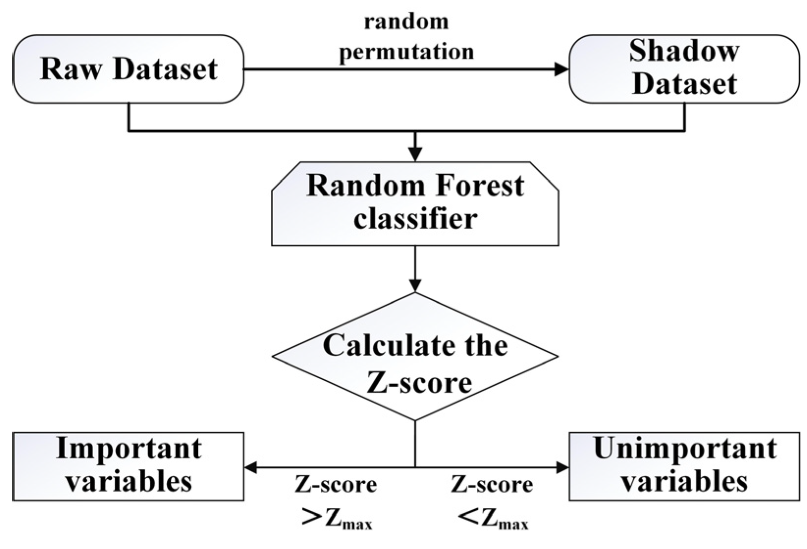
Due to the redundancy and high autocorrelation of certain predictive variables, they may not provide effective information for predicting SOC content [14]. Therefore, we used Boruta to select the feature variables [42]. The main principle of Boruta is to randomly generate shadow variables by transforming the original variables (Figure 2). The shadow variables and original variables were input into a random forest classifier to calculate the Z-scores. The maximum Z-score among the shadow variables is referred to as “Z_max”. Variables with Z-scores higher than Z_max are retained, while those with Z-scores lower than Z_max are discarded. This process is repeated until all variables have been screened. The results of variable selection are presented in

Table 3. Variables screening results.

Model Factor Database	Screening Result
BBlue, BGreen, BRed, BNIR, BSWIR1, BSWIR2, NDWI, MNDWI, NDVI, RVI, EVI, NDI, DVI, RDVI, SAVI, TSAVI, MSAVI, CVI, WRI, NDSI, KNDVI, Mean, Variance, Homogeneity, Contrast, Dissimilarity, Entropy, Second moment, Correlation, MAT, MAP	BBlue, BGreen, BRed, BNIR, BSWIR1, BSWIR2, NDWI, MNDWI, NDVI, RVI, EVI, NDI, DVI, RDVI, SAVI, TSAVI, MSAVI, CVI, WRI, NDSI, KNDVI, Variance, MAT, MAP

.

2.3.2. Random Forest

Random Forest (RF)is an ML model based on decision trees. The model generates multiple training datasets by performing bootstrap sampling (random sampling with replacement) on the original dataset and uses the decision tree method to model each training dataset. These decision trees are combined into a predictive model comprising multiple decision trees, offering a single prediction target for data forecasting. The final forecast result is obtained by averaging the predictions of all individual decision trees [43]. It has certain advantages in handling multivariate nonlinear data, such as robustness in reducing overfitting, strong noise resistance, and higher accuracy. This is particularly important for time-series remote sensing data and has been widely applied in soil property research.

2.3.3. Boosted Regression Tree

Boosted Regression Tree (BRT)is an ML model that combines regression trees and boosting models [44]. It combines multiple weak regression trees into a robust predictive model, with each individual tree capturing underlying trends within the data. By iteratively applying binary recursive partitioning, a regression model based on classification and regression trees is fitted. Based on the prediction results of the previous model, the weights of the data points are reallocated, assigning greater weight to those that were incorrectly predicted in the earlier iteration. By fitting the residuals from previous iterations, the final model aggregates the weighted predictions of all weak regression trees to generate an overall prediction of the target variable, thereby enhancing the model’s stability and accuracy.

2.3.4. EXtreme Gradient Boosting

EXtreme Gradient Boosting (XGBoost)is a model based on the gradient boosting decision tree framework. It improves upon the gradient boosting decision tree model by performing a second-order Taylor expansion of the loss function and adding a regularization term to the loss function. Through iterative combination of multiple models with lower accuracy into a single high-accuracy model [45], XGBoost minimizes uncertainty, resulting in improved accuracy and reduced susceptibility to overfitting. The new loss function is:

$$L\mathrm{oss}\left(y,F\left(x\right)\right)={\displaystyle {\sum }_i^{n}l\left(y,F\left(x\right)\right)+{\displaystyle {\sum }_m^M\left(f_m\right)}}$$

(1)

where Ω(fm) is the regularization term for the m iteration.

The above models were implemented using the “train” function from the “caret” package in R (v4.2.3). A grid search method was used to optimize the main hyperparameters of the machine learning models, aiming to reduce model errors and improve model performance.

2.3.5. Model Validation

Leave-one-out cross-validation was used to perform cross-validation on the SOC content prediction model. This method divides the dataset into K subsets, where K is the total number of data points in the dataset. Each time, one subset is selected as the test set, and the remaining subsets are used as the training set. The mean of all test results was taken as the result [46].

The coefficient of determination (R²), mean absolute error (MAE), and root mean squared error (RMSE) were used to evaluate the accuracy of the model [47]. In addition, the Willmott concordance index (d-Willmott) evaluates whether the model fits in relation to the observed values, reflecting the degree of agreement between the predicted and observed values [48]. The calculation formulas for these evaluation metrics are as follows:

$$R^2={\displaystyle \frac{{\displaystyle {\sum }_{i=1}^n{\left({\widehat{y}}_i-\overline{y}\right)}^2}}{{\displaystyle {\sum }_{i=1}^n{\left(y_i-\overline{y}\right)}^2}}}$$

(2)

$$MAE={\displaystyle \frac{{\displaystyle {\sum }_{i=1}^n\left|{\widehat{y}}_i-y_i\right|}}{n}}$$

(3)

$$RMSE=\sqrt{{\displaystyle \frac{{\displaystyle {\sum }_{i=1}^n{\left({\widehat{y}}_i-y_i\right)}^2}}{n}}}$$

(4)

$$d\text{-}Willmott={\displaystyle \frac{{\displaystyle \sum {\left({\widehat{y}}_i-y_i\right)}^2}}{{\displaystyle \sum {\left(\left|{\widehat{y}}_i-\overline{y}\right|+\left|y_i-\overline{y}\right|\right)}^2}}}$$

(5)

where $n$ is the number of samples, $\widehat{y_i}$ and $y_i$ are the predicted and observed values at the site $i$, respectively, and $\overline{y}$ represents the mean values of the SOC content.

3. Results

3.1. Spatiotemporal Evolution Characteristics of Tidal Flat Reclamation

3.1.1. Classification Results of Western Coastal Region of the Bohai Rim

To obtain the spatial distribution of tidal flat reclamation, land cover classification was conducted using Landsat images from 2000 to 2020 (Figure 1c–g). The overall classification accuracy exceeded 85.00%, with a kappa coefficient greater than 0.83. Specifically, from 2000 to 2020, the user’s accuracy for tidal flats consistently exceeded 0.85, while the producer’s accuracy was above 0.75, providing a reliable accuracy foundation for subsequent study (

Table 4. Evaluation of the classification precision.

Year	Overall Classification Accuracy	Kappa Coefficient	User’s Accuracy for Tidal Flats	Producer’s Accuracy for Tidal Flats
2000	0.86	0.84	0.86	0.78
2005	0.86	0.84	0.88	0.85
2010	0.87	0.85	0.88	0.75
2015	0.86	0.84	0.88	0.82
2020	0.88	0.86	0.88	0.78

).

Based on the land cover types in the western coastal region of the Bohai Rim, tidal flat reclamation was defined as the conversion of tidal flats into farmlands, forest lands, grasslands, marshes, aquaculture ponds, residential lands, transportation lands, industrial sites, and bare lands. The spatial distribution of tidal flat reclamation was extracted for four different periods. A quantitative analysis was conducted on the spatial distribution features of tidal flat reclamation across different periods (

Table 5. The demarcation of different reclamation periods.

Date	Reclamation Periods	Number of Periods
2015–2020	<5 years	Period I
2010–2020	5–10 years	Period II
2005–2020	10–15 years	Period III
2000–2020	15–20 years	Period IV

Notes: reclamation periods, reclamation time range from the year of reclamation to the reference year (2020); number of periods, stage groups classified by reclamation year.

). Detailed information on the land cover results is provided in the Supplementary Materials.

3.1.2. Spatiotemporal Distribution and Change in Tidal Flat Reclamation

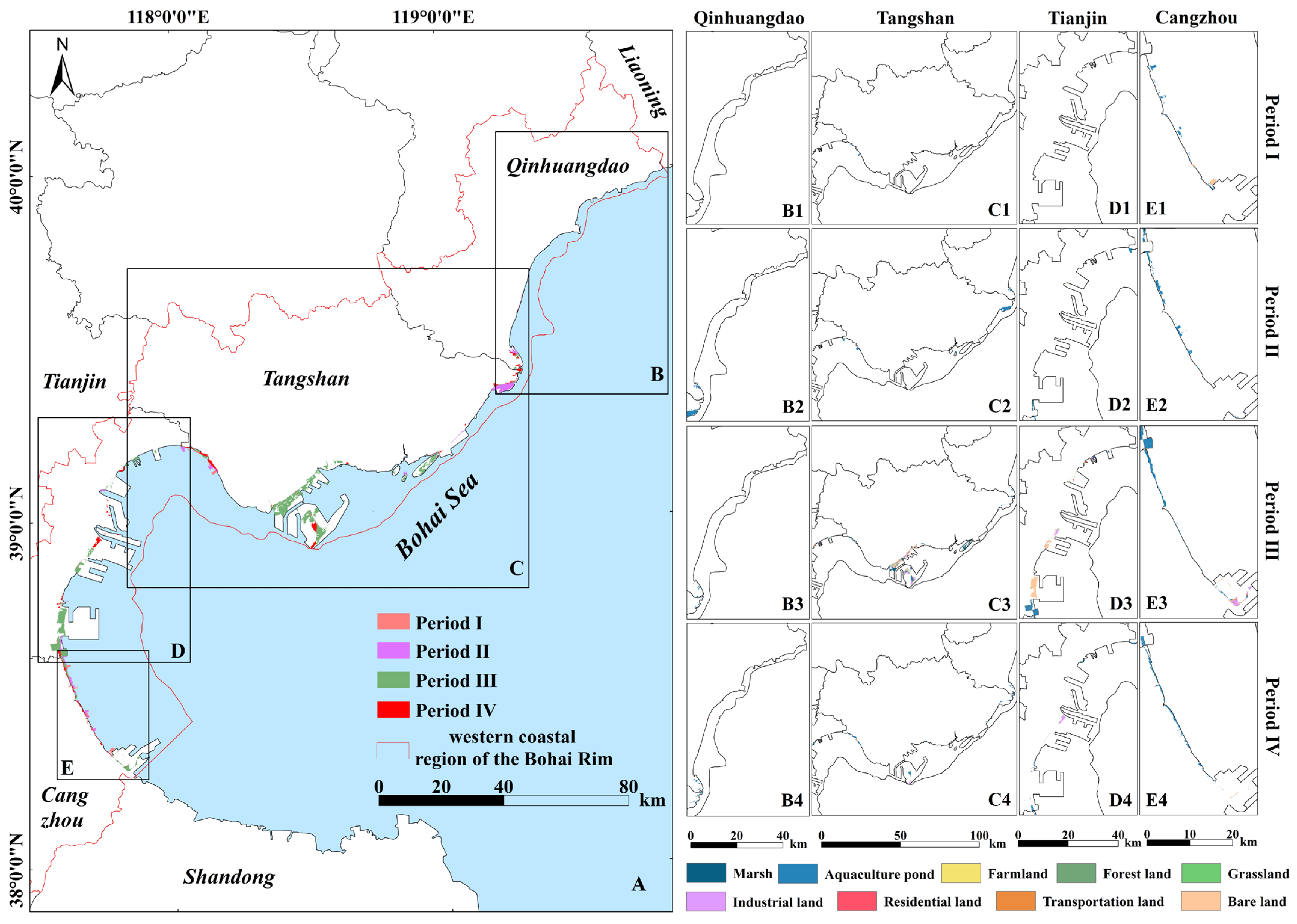
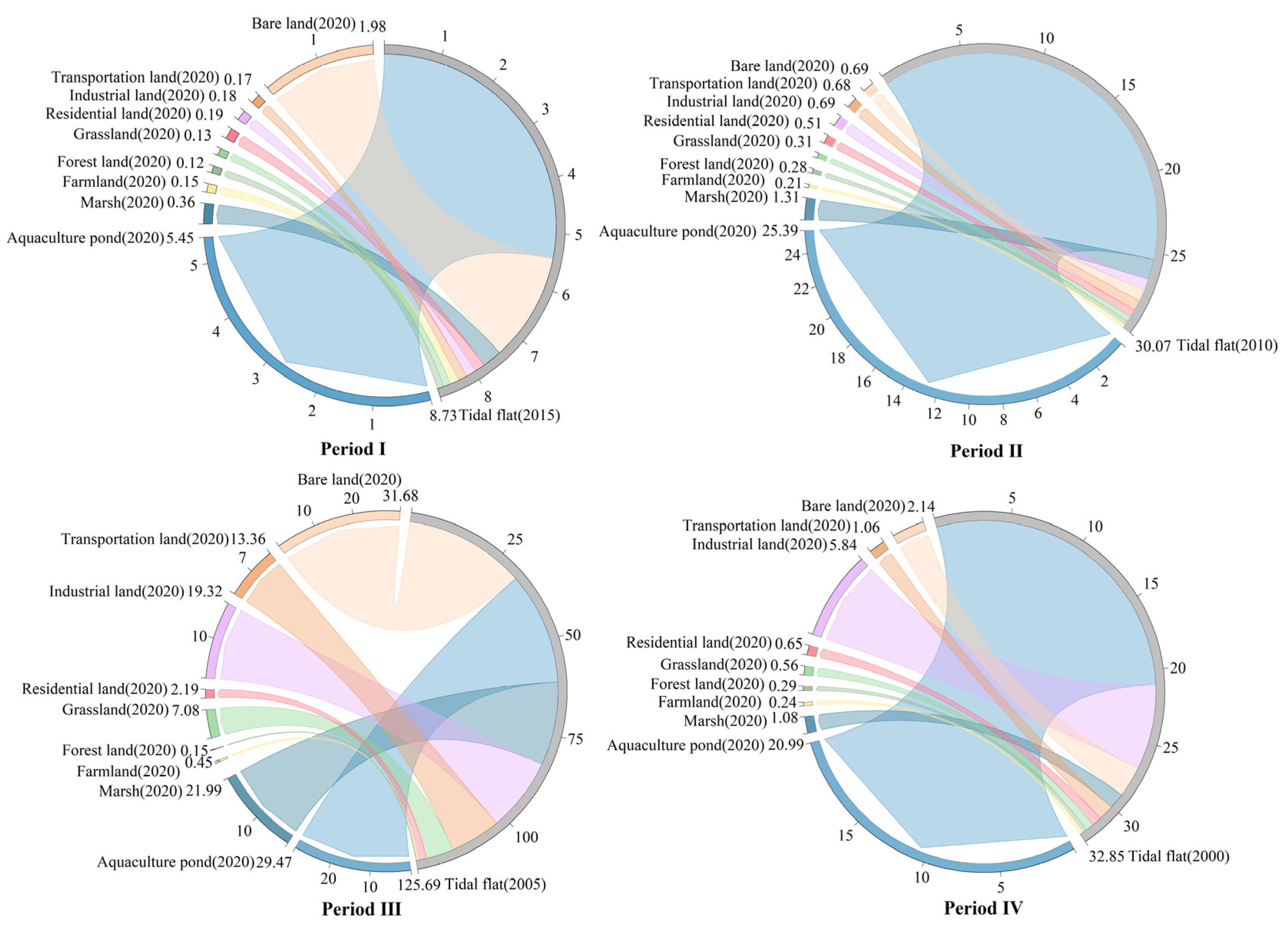
Tidal flat reclamation was primarily converted into aquaculture ponds, bare lands, and marshes, accounting for over 66.00% of the total reclaimed area (Figure 3 and Figure 4). From Period I to Period IV, the area of tidal flat reclamation exhibited an increasing tendency, peaking at 125.69 km² in Period III. The reclamation regions were mainly located in the coastal regions of Tangshan, Tianjin, and Cangzhou. In the coastal region of Qinhuangdao, tidal flat reclamation was considerably restricted, with only a small portion located near the Luanhe estuary (Figure 3B1–B4). During Period I, the area of tidal flat reclamation decreased because of the enforcement of protection measures.

The area of tidal flat reclamation exhibited an increasing tendency with the increase in reclamation periods, reaching its peak in Period III. Notably, the reclamation areas of marshes and grasslands in Period III were substantially larger than those in other reclamation periods. Over the progression of reclamation periods, the area of tidal flat reclamation converted to forest lands and bare lands fluctuated but demonstrated an overall increasing trend. Among all reclamation types, bare lands emerged as the dominant land cover type in Period III, with the largest area devoted to this use, predominantly in Tianjin’s coastal region (Figure 3).

3.2. Prediction Model Performance for SOC Content

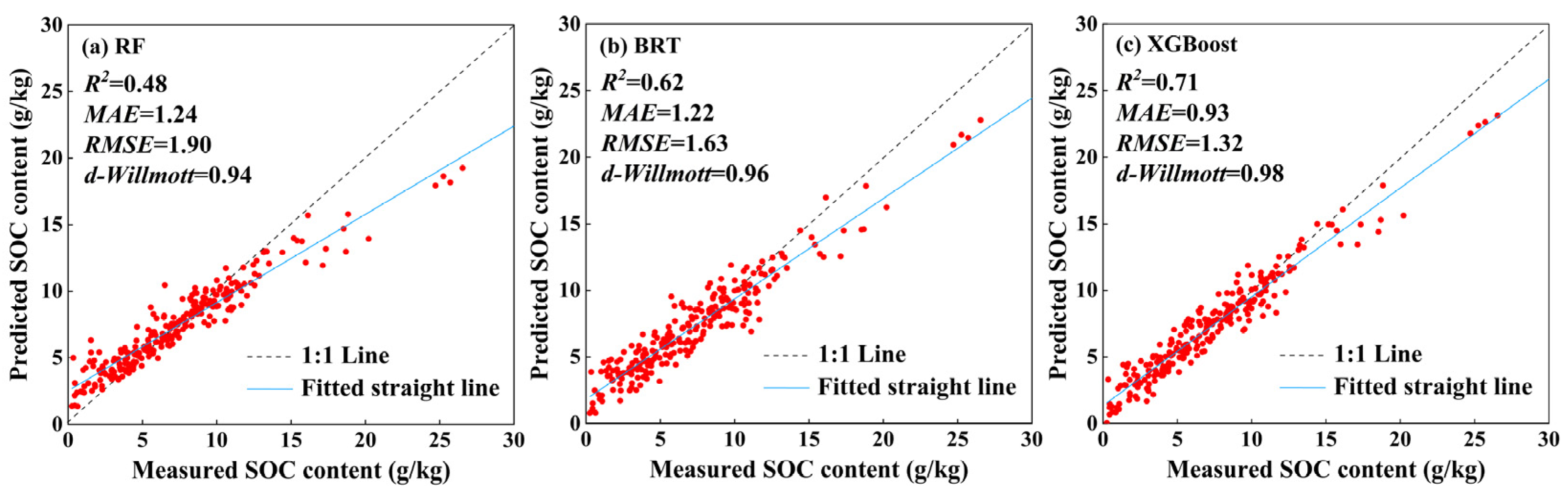
According to the chosen model factor database (Table 3), RF, BRT, and XGBoost models were employed to predict SOC content. The comparative study revealed that all models demonstrated strong agreement between the predicted and observed SOC contents, with d-Willmott values surpassing 0.94 (Figure 5). The performance ranking of the models was as follows: XGBoost > BRT > RF. The R² of the XGBoost model was 147.92% and 114.52% of the RF and BRT models, respectively. Meanwhile, the MAE of the XGBoost model was 75.00% and 76.23% for the two, respectively. The RMSE were 69.47% and 80.98% for the two, respectively. Additionally, the XGBoost model exhibited closer to the 1:1 line between the predicted and observed values. Therefore, the XGBoost model was selected for predicting SOC content.

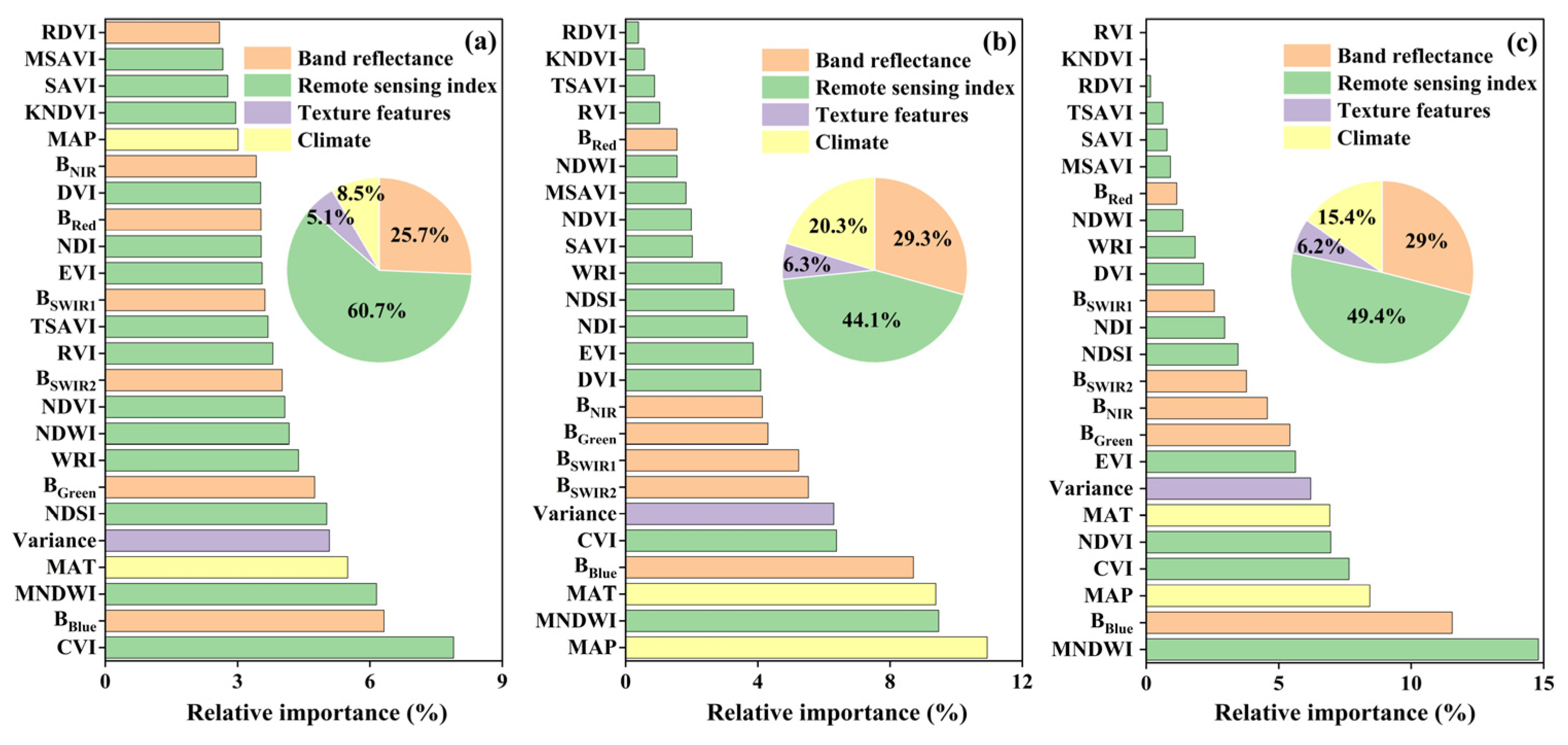
The variables were prioritized according to their relative importance in the three SOC content prediction models (Figure 6). The results indicated that remote sensing indices were the primary explanatory variables, accounting for 60.70%, 44.10%, and 49.40% of the explained variation in the RF, BRT, and XGBoost models, respectively. Band reflectance and climatic variables followed in importance, whereas texture features showed the lowest relative importance. The rankings of variable relative importance exhibited minor variations across the three models. CVI (7.89%), MAP (10.94%), and MNDWI (14.80%) ranked first in the RF, BRT, and XGBoost models, respectively. MNDWI consistently demonstrated strong predictive power, ranking among the top three variables in all models and serving as the most important variable in the XGBoost model. Although texture features comprised only one predictor variable, they consistently ranked within the top ten across all three models. Among the band reflectance variables, B_Blue showed higher relative importance than the other predictors.

3.3. Impact of Tidal Flat Reclamation on SOC Content Change

3.3.1. Spatiotemporal Distribution of SOC Content in Tidal Flats

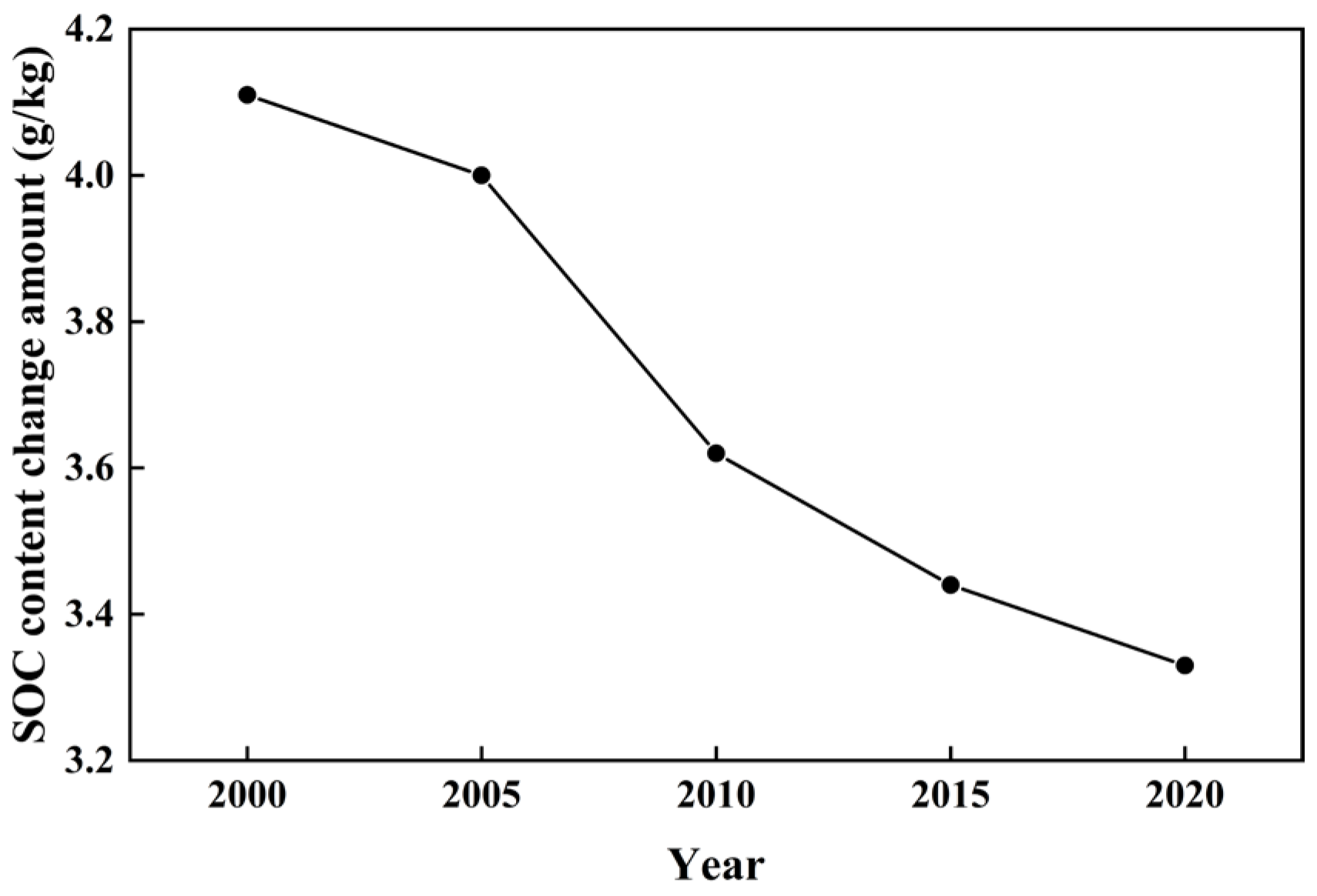
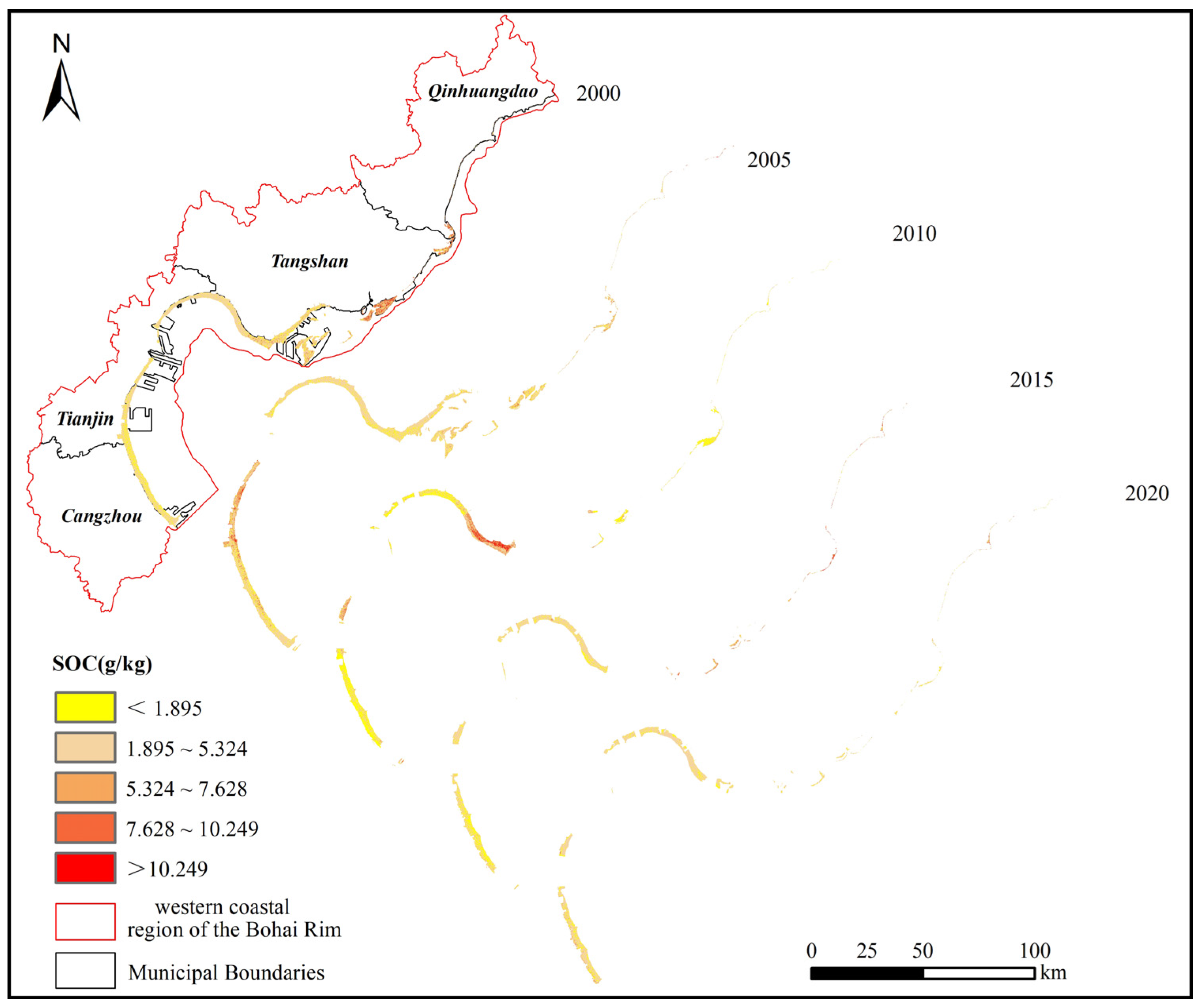
From 2000 to 2020, the SOC content in the coastal tidal flats of the western Bohai Rim exhibited a decreasing trend, falling from 4.11 g/kg in 2000 to 3.33 g/kg in 2020, indicating a decrease of 18.98% (Figure 7). The regions with the most significant decreases in SOC content were primarily located in the coastal region of Tangshan. Between 2000 and 2005, the decrease in tidal flat SOC content was relatively small, at 0.11 g/kg. The regions with the most significant decreases in SOC content were primarily located around the Luanhe estuary and the eastern coastal region of Tangshan (Figure 8). From 2005 to 2010, the reduction in tidal flat SOC content reached its maximum, with a decrease of 0.38 g/kg. The regions with the most significant reduction in tidal flat SOC content were in the coastal regions of Cangzhou and Qinhuangdao. In contrast, SOC content increased in the coastal regions of Tangshan. From 2010 to 2015, the SOC content in tidal flats decreased by 0.18 g/kg. The regions exhibiting the most significant SOC loss were primarily located in the coastal regions of Tangshan and Tianjin. From 2015 to 2020, the rate of SOC content declined slowed, with a decrease of 0.11 g/kg, the same as that from 2000 to 2005.

3.3.2. SOC Content Changes Across Different Reclamation Types and Periods

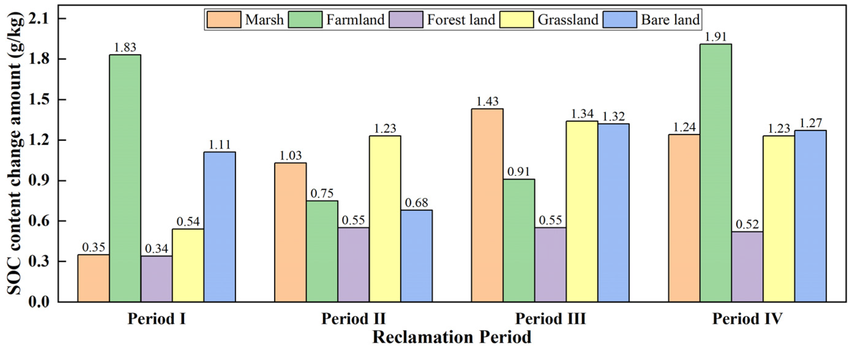
An analysis of the impact of different reclamation types on tidal flat SOC content within the same reclamation periods revealed that converting tidal flats into marshes, grasslands, forest lands, farmlands, and bare lands led to increases in SOC content (Figure 9). In Period IV, the regions where tidal flats were converted into farmlands exhibited the highest increase in SOC content, reaching 1.91 g/kg. However, the increase in SOC content was lowest in regions where tidal flats were converted to forest lands, with an increment of only 0.52 g/kg. In Period II, the greatest increase in SOC content was observed in regions where tidal flats were converted to grasslands, while the smallest increase was still found in regions converted to forest lands. In Period III, the tendency in SOC content changes was consistent with that in Period I. However, reclamation resulted in a continuous decline in SOC content in tidal flat regions, decreasing from 4.11 g/kg in 2000 to 3.33 g/kg in 2020.

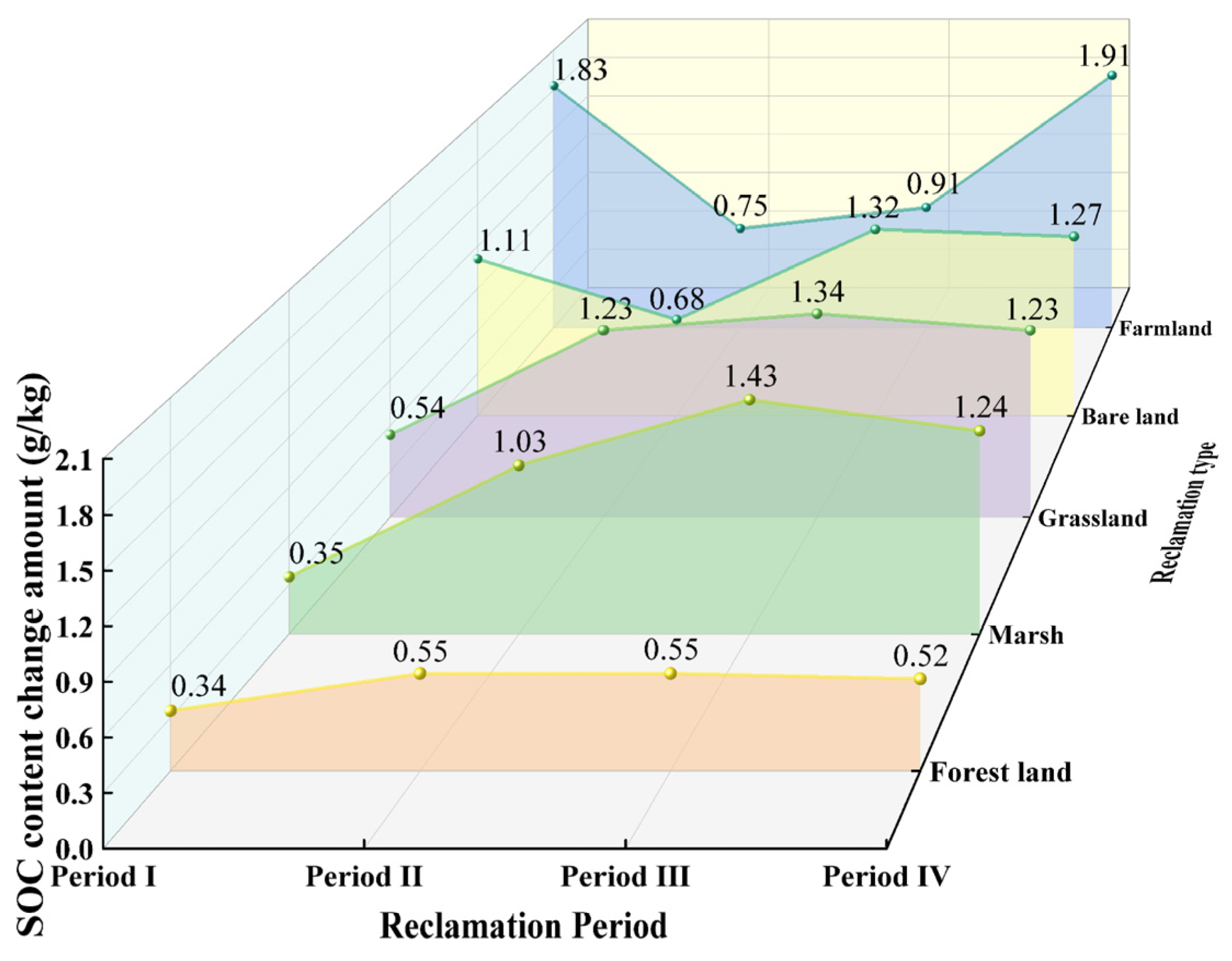
An analysis of the effects of the same reclamation type across different periods on tidal flat SOC content revealed a consistent trend in regions converted to marshes, forest lands, and grasslands, where SOC content initially increased and then decreased, peaking in Period III (Figure 10). Specifically, compared to Period III, the increase in SOC content in regions where tidal flats were converted to marshes declined in Period IV but remained higher than in Periods I and II. From Period II to IV, the SOC content in grassland-converted regions remained stable, with a mean increase of 1.26 g/kg. In regions where tidal flats were converted to forest lands, the SOC content increased by 0.55 g/kg in both Period II and Period III. Influenced by vegetation succession, the SOC content in regions where tidal flats were converted to farmland showed a U-shaped increasing trend. During Period II, the increase in SOC content was relatively low, at 0.75 g/kg. Due to the conversion of tidal flats to bare lands, which were partly used for industrial development or subjected to other anthropogenic disturbances, the SOC content exhibited a fluctuating increasing tendency.

4. Discussion

4.1. Evaluating the Predictive Performance of Machine Learning Models

Among the three predictive models, the d-Willmott values were all greater than 0.94, indicating that all models exhibited good agreement between the predicted and observed SOC contents. XGBoost exhibited the best performance, accounting for 71.00% of the variability in SOC content, followed by BRT and RF. The RF model’s predictions are derived from the averaged outputs of multiple independent decision trees, which makes its prediction of SOC content relatively conservative [49]. The BRT model effectively captures intricate nonlinear relationships and can automatically accommodate for interactions among predictive variables [50]. In contrast to BRT, XGBoost uses second-order Taylor expansion of the loss function and integrates regularization component to enhance model generalization [51]. This enhanced the model performance, with R² increasing by 14.52%, and MAE and RMSE decreasing by 23.77% and 19.02%, respectively.

In large regional soil parameter prediction studies, the R² values of the optimal models generally range between 0.70 and 0.75, which is consistent with the model performance observed in this study [52,53]. A comparison with related studies in the same region reveals that the model constructed in this study demonstrates superior prediction accuracy. Researchers constructed soil total nitrogen (STN) prediction models for northeastern Hebei Province based on Landsat-8 imagery, in which the RF and XGBoost models explained 44.60% and 49.80% of STN variability, respectively [49]. All values are lower than the corresponding values of 48.00% and 71.00% in this study. This is primarily because their model only considered band reflectance and remote sensing indices, without accounting for the sensitivity of soil parameters to texture features and climatic variables.

In the construction of predictive models, remote sensing indices and band reflectance proved more important than texture features and climatic variables. This is mainly because they provide characteristic information related to vegetation and soil properties [54]. Differences in SOC content affect the absorption and reflectance features of soil across different wavelengths, thereby being reflected in the band reflectance [55]. Texture features are also important predictors of SOC content, as they effectively complement spatial structural information [56]. In addition, precipitation and temperature affect SOC content by altering soil hydrothermal conditions and regulating microbial decomposition [57].

The models show a notable similarity in relative importance. For example, 6 of the top 10 important predictor variables were repeated among the three models, namely CVI, B_Blue, MNDWI, MAT, variance, and B_Green. Moreover, we also observed that in models with higher prediction accuracy, MNDWI ranked higher and was even top-ranked in the XGBoost model. This is probably because MNDWI can accurately capture subtle variations in soil moisture [40]. These moisture variations reflect changes in soil environmental conditions, which are often closely related to the processes of SOC formation, transformation, and storage, thus providing crucial information for predicting SOC content [58]. Additionally, MNDWI reduces the impact of vegetation and background, enabling clearer observation of spectral features related to soil moisture and SOC. This is crucial for predicting SOC content in areas with vegetation cover.

4.2. Assessing the Accuracy and Constraints of Historical SOC Content Reconstruction

In the qualitative approach, previous studies have shown the mean SOC content in the Luan River catchment was 6.23 g/kg in 2016 [59]. The mean SOC content for the corresponding region in 2015 was 6.13 g/kg. The close proximity of these two values suggests a high prediction accuracy. Based on the typical soil organic matter (SOM) data from the Second National Soil Survey, the SOC content within Hebei province was obtained using the standard conversion formula between SOM and SOC, a value of 7.39 g/kg. Extracting the SOC content for 2000 from the coastal regions of Qinhuangdao, Tangshan, and Cangzhou, the average value was 7.26 g/kg, which is 1.76% lower than the provincial average (Δ = 0.13 g/kg). This is mainly because frequent salinization in coastal regions impedes organic matter formation. Moreover, the litter input from vegetation is also lower in coastal regions. From the predicted SOC content in 2010, the results of this study exhibit a certain degree of similarity with previous study findings, thereby confirming the reliability of the historical SOC content reconstruction [60].

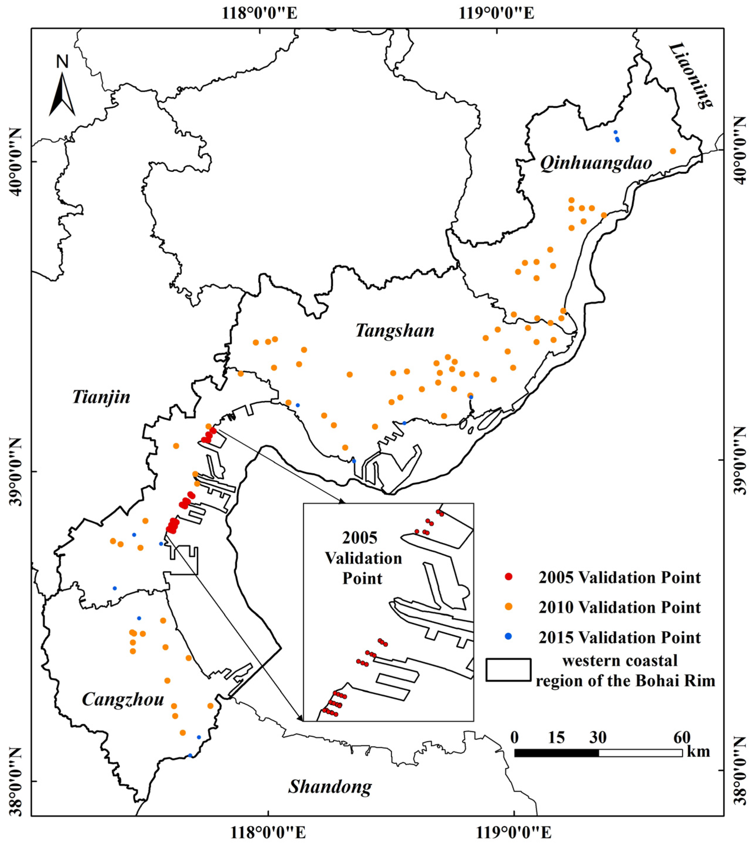
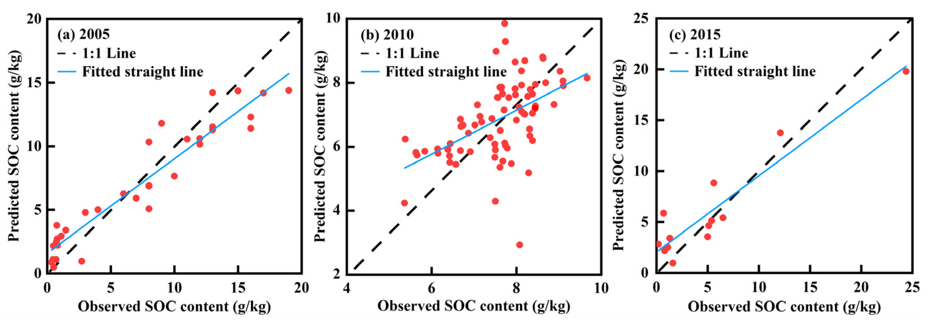
Validation data for the quantitative approach were obtained from the National Earth System Science Data Center (https://www.geodata.cn, accessed on 7 February 2024). Scatter plots were created using the SOC validation data from verification points and the results of this study (Figure 11 and Figure 12). The findings demonstrate that these points are quite close to the 1:1 line. The prediction accuracy for 2005 was greater than that for 2010 and equivalent to that for 2015, primarily because the validation data for both 2005 and 2015 were acquired from field measurements. In particular, the validation data for 2005 were collected from intertidal zones, where the soil’s physicochemical properties closely match those of the sampling regions in this study. In contrast, the 2010 data were produced from national-scale predictions, which inherently possess lower accuracy compared to field-observed observations.

Although the historical reconstruction and inversion of SOC content were effectively carried out, certain limitations persist. From a theoretical and methodological perspective, the space-for-time substitution approach has strong practical significance in the absence of long-term monitoring data. Its reliability is based on a key assumption: that the spatially nonlinear mapping relationship between SOC and environmental covariates remains relatively stable over the 20-year period [61]. However, over this time scale, environmental factors such as temperature and precipitation may change substantially, resulting in inconsistencies between the environmental conditions of the historical and current periods, thereby weakening or even destroying the space–time equivalence assumption [62,63]. In addition, land cover changes caused by reclamation and the lag effects of biogeochemical processes may further introduce uncertainty [64,65]. Previous studies have shown that the uncertainties mentioned above can be mitigated, to some extent, by incorporating dynamic covariates, integrating multi-source data, and applying joint modeling across multiple time periods [64,66,67]. Fundamentally, the reliability of this approach still depends on the continuous validation and calibration of the model using more long-term monitoring data. In terms of data, variations in data quality and inconsistencies in sensor types within time-series remote sensing data may lead to a decline in the model’s predictive performance during temporal transfer. Furthermore, the absence of systematic, temporally continuous, and complete field-based soil measurements presents challenges for the reliable validation of model performance across different periods.

4.3. Impacts of Tidal Flat Reclamation on SOC Content

The average increases in SOC content in areas where tidal flats were reclaimed and converted into marshes, grasslands, forest lands, farmlands, and bare lands were 1.01 g/kg, 1.09 g/kg, 0.49 g/kg, 1.35 g/kg, and 1.10 g/kg, respectively (Figure 9). Among them, regions converted to farmlands showed the highest increase in SOC content, while those converted to forest lands showed the lowest increase.

When tidal flats are reclaimed and converted into forest lands and grasslands, this generally indicates a higher level of vegetation cover. During their growth, trees and herbaceous plants produce substantial amounts of litter, consistently providing organic matter to the soil and thereby increasing SOC content [68]. Nevertheless, unique saline–alkaline conditions of coastal regions are often unfavorable for the growth of woody vegetation. Furthermore, due to the resistant nature of lignin in tree litter, its decomposition and conversion into SOC require an extended duration [69]. Therefore, in the short term, regions where tidal flats are converted into forest lands exhibit the lowest increase in SOC content. When tidal flats are reclaimed and converted into marshes, the resulting ecosystem, characterized by abundant moisture and relatively low oxygen availability, slows the decomposition of organic matter [70]. This slower decomposition facilitates the accumulation of organic material, thereby contributing to an increase in SOC content [71]. In contrast, grassland ecosystems often exhibit superior soil aeration, which supports higher microbial activity, promotes the decomposition of organic matter, and enhances soil respiration intensity [72]. As a result, the respiratory intensity of grassland ecosystems tends to be higher than that of marsh wetlands, leading to a lower increase in SOC content in regions converted into marshes compared to those converted into grasslands. In their natural state, bare lands may undergo natural vegetation growth and succession. Although these ecological processes progress relatively slowly, they can progressively boost the accumulation of SOC over time. After the reclamation of tidal flats into farmlands, long-term cultivation and fertilization have increased SOC content through crop roots and residues [73]. Moreover, appropriate field management practices can enhance SOC content by promoting microbial metabolism [74]. However, tidal flat reclamation leads to a continuous decline in SOC content within the existing tidal flats, primarily due to alterations in the original hydrological conditions. These changes affect microbial activity and accelerate the decomposition rate of organic carbon. Reclamation activities sometimes obstruct tidal channels, thereby reducing hydrological exchange between seawater and tidal flats. This reduction in exchange limits carbon input into the tidal flat ecosystem, ultimately hindering the accumulation of SOC.

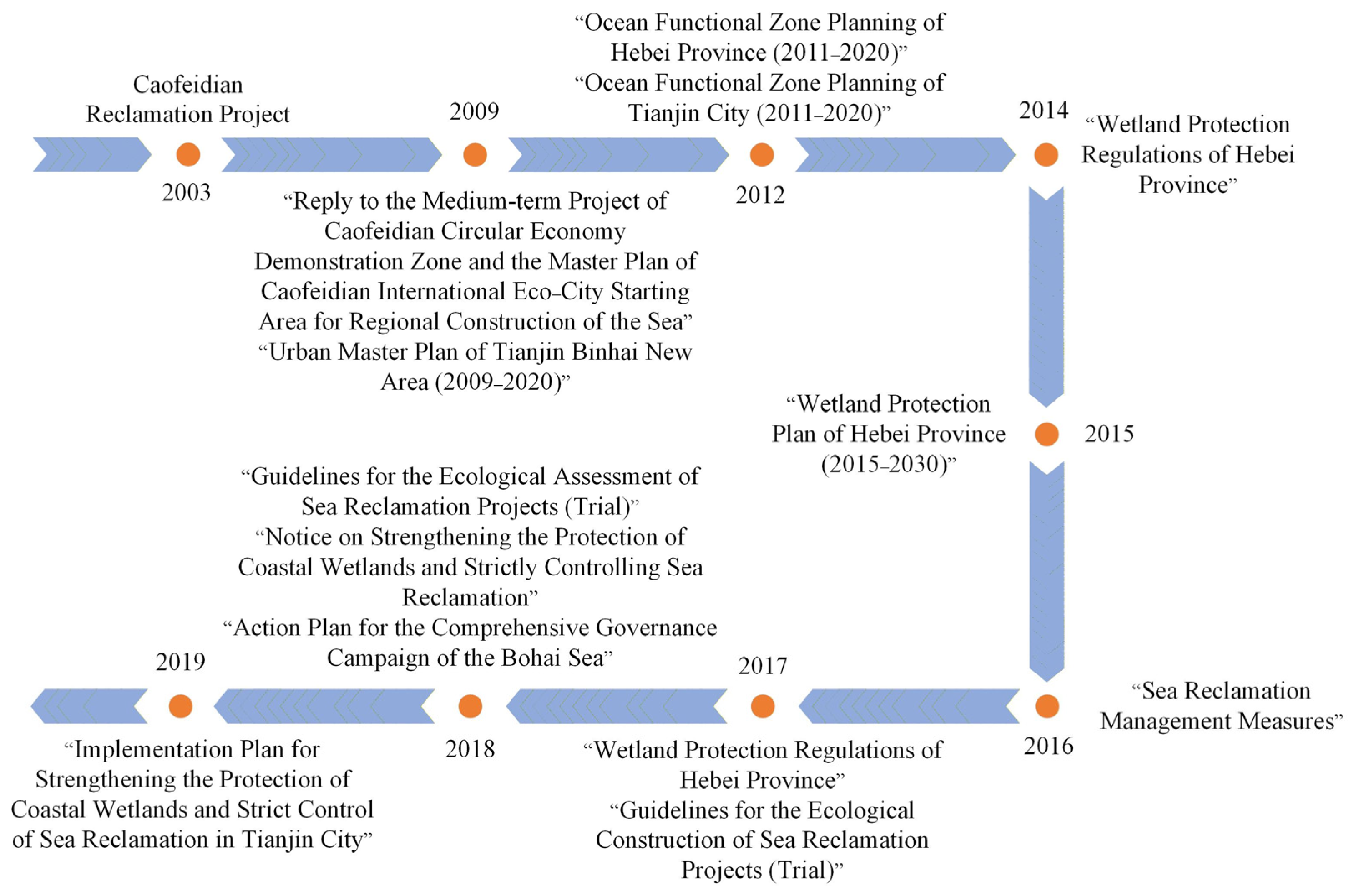
In Period II, the regions where tidal flats were converted into forest lands, farmlands and bare lands exhibited the smallest increase in SOC content, while the lowest SOC content increment for regions converted into marshes, forest lands, and grasslands occurred in Period I. The observed low increase in SOC content during the early stages of reclamation can be attributed to the lag effect inherent in reclamation processes, which produces a delayed response in the accumulation of SOC. Moreover, during the early stages of reclamation, several policies were introduced to strictly regulate the total area of reclamation, focusing on restoring the coastal ecological environment (Figure 13). As a result, the rate of SOC content increase decreased. SOC content changes are primarily driven by the cumulative effect of time. Therefore, the peak increase in SOC content within tidal flat reclamation regions occurs during both Period III and Period IV. Except for the regions where tidal flats were converted into farmlands, where the peak increase in SOC content occurs in Period IV, the peak increases in SOC content for other land cover types occur in Period III.

5. Conclusions

Tidal flat reclamation was primarily converted into aquaculture ponds, bare lands, marshes, industrial lands, and transportation lands. The tidal flat reclamation area exhibited an increasing trend with the increase in reclamation periods, reaching a peak of 125.69 km² in Period III.

The RF, BRT, and XGBoost models all accurately predicted SOC content, with the XGBoost model achieving an R² as high as 0.71. Remote sensing indices were the most important factors, accounting for over 44.00%.

Between 2000 and 2020, the SOC content in regions where tidal flats were converted to marshes, forest lands, grasslands, farmlands, and bare lands increased by 29.18%, 11.85%, 30.98%, 45.91%, and 29.40%, respectively. However, tidal flat reclamation led to a decrease of 0.78 g/kg (18.98%) in the SOC content of the existing tidal flats.

Nonetheless, certain limitations persist in the current study. The restricted accessibility of historical remote sensing images and SOC data adversely affects model development and outcome verification. In the future, we will integrate multi-source remote sensing data to improve the temporal continuity and spatial resolution of historical imagery. We will develop inversion models with temporal dynamic adaptability, such as deep-learning-based temporal models and ensemble learning frameworks, to enhance the robustness of the models against fluctuations in the quality of historical remote sensing data.

References

1. Falahatkar, S.; Hosseini, S.M.; Ayoubi, S.; Salmanmahiny, A. Predicting soil organic carbon density using auxiliary environmental variables in northern Iran. Arch. Agron. Soil Sci. 2016, 62, 375–393. [Google Scholar] [CrossRef]
2. Chmura, G.L.; Anisfeld, S.C.; Cahoon, D.R.; Lynch, J.C. Global carbon sequestration in tidal, saline wetland soils. Glob. Biogeochem. Cycles 2003, 17, 1111. [Google Scholar] [CrossRef]
3. Xiao, R.; Yu, X.Y.; Xiang, T.; Zhang, Z.H.; Wang, X.; Wu, J.G. Exploring the coordination between physical space expansion and social space growth of China’s urban agglomerations based on hierarchical analysis. Land Use Policy 2021, 109, 105700. [Google Scholar] [CrossRef]
4. Zhao, S.S.; Liu, Y.X.; Li, M.C.; Sun, C.; Zhou, M.X.; Zhang, H.X. Analysis of Jiangsu tidal flats reclamation from 1974 to 2012 using remote sensing. China Ocean Eng. 2015, 29, 143–154. [Google Scholar] [CrossRef]
5. He, T.T.; Xia, Q.; Zhang, H.; Zheng, Q.; Zhu, H.T.; Deng, X.S.; Zhang, Y.F. Development of a tidal flat recognition index based on multispectral images for mapping tidal flats. Ecol. Indic. 2023, 157, 111218. [Google Scholar] [CrossRef]
6. Man, W.D.; Yu, H.; Li, L.; Liu, M.Y.; Mao, D.H.; Ren, C.i.; Wang, Z.M.; Jia, M.M.; Miao, Z.H.; Lu, C.; et al. Spatial Expansion and Soil Organic Carbon Storage Changes of Croplands in the Sanjiang Plain, China. Sustainability 2017, 9, 563. [Google Scholar] [CrossRef]
7. Wang, X.P.; Yao, R.J.; Yang, J.S.; Xie, W.P.; Chen, C.; Zhang, X.; Wang, F.; Li, W.P. Soil organic carbon distribution and storage along reclamation chronosequences in a typical coastal farming area, Eastern China. Environ. Earth Sci. 2023, 82, 170. [Google Scholar] [CrossRef]
8. Li, J.G.; Yang, W.H.; Li, Q.; Pu, L.J.; Xu, Y.; Zhang, Z.Q.; Liu, L.L. Effect of reclamation on soil organic carbon pools in coastal areas of eastern China. Front. Earth Sci. 2018, 12, 339–348. [Google Scholar] [CrossRef]
9. Wan, S.; Mou, X.J.; Liu, X.T. Effects of Reclamation on Soil Carbon and Nitrogen in Coastal Wetlands of Liaohe River Delta, China. Chin. Geogr. Sci. 2018, 28, 443–455. [Google Scholar] [CrossRef]
10. Zhou, T.; Geng, Y.J.; Chen, J.; Liu, M.M.; Haase, D.; Lausch, A. Mapping soil organic carbon content using multi-source remote sensing variables in the Heihe River Basin in China. Ecol. Indic. 2020, 114, 106288. [Google Scholar] [CrossRef]
11. Chi, Y.; Liu, D.H.; Xie, Z.L. Zonal simulations for soil organic carbon mapping in coastal wetlands. Ecol. Indic. 2021, 132, 108291. [Google Scholar] [CrossRef]
12. Zeraatpisheh, M.; Garosi, Y.; Reza Owliaie, H.; Ayoubi, S.; Taghizadeh-Mehrjardi, R.; Scholten, T.; Xu, M. Improving the spatial prediction of soil organic carbon using environmental covariates selection: A comparison of a group of environmental covariates. CATENA 2022, 208, 105723. [Google Scholar] [CrossRef]
13. Garosi, Y.; Ayoubi, S.; Nussbaum, M.; Sheklabadi, M. Effects of different sources and spatial resolutions of environmental covariates on predicting soil organic carbon using machine learning in a semi-arid region of Iran. Geoderma Reg. 2022, 29, e00513. [Google Scholar] [CrossRef]
14. Zhang, Y.B.; Kou, C.Y.; Liu, M.Y.; Man, W.D.; Li, F.P.; Lu, C.Y.; Song, J.R.; Song, T.L.; Zhang, Q.W.; Li, X.; et al. Estimation of Coastal Wetland Soil Organic Carbon Content in Western Bohai Bay Using Remote Sensing, Climate, and Topographic Data. Remote Sens. 2023, 15, 4241. [Google Scholar] [CrossRef]
15. Xie, B.Q.; Ding, J.L.; Ge, X.Y.; Li, X.H.; Han, L.J.; Wang, Z. Estimation of Soil Organic Carbon Content in the Ebinur Lake Wetland, Xinjiang, China, Based on Multisource Remote Sensing Data and Ensemble Learning Algorithms. Sensors 2022, 22, 2685. [Google Scholar] [CrossRef]
16. Guo, L.; Fu, P.; Shi, T.Z.; Chen, Y.Y.; Zeng, C.; Zhang, H.T.; Wang, S.Q. Exploring influence factors in mapping soil organic carbon on low-relief agricultural lands using time series of remote sensing data. Soil Tillage Res. 2021, 210, 104982. [Google Scholar] [CrossRef]
17. Yang, J.Y.; Fan, J.J.; Lan, Z.F.; Mu, X.M.; Wu, Y.P.; Xin, Z.B.; Miping, P.Q.; Zhao, G.J. Improved Surface Soil Organic Carbon Mapping of SoilGrids250m Using Sentinel-2 Spectral Images in the Qinghai–Tibetan Plateau. Remote Sens. 2023, 15, 114. [Google Scholar] [CrossRef]
18. Chi, Y.; Liu, D.H. Mapping the Spatiotemporal Pattern of Sandy Island Ecosystem Health during the Last Decades Based on Remote Sensing. Remote Sens. 2022, 14, 5208. [Google Scholar] [CrossRef]
19. Zhang, S.; Tian, J.; Lu, X.; Tian, Q.J. Temporal and spatial dynamics distribution of organic carbon content of surface soil in coastal wetlands of Yancheng, China from 2000 to 2022 based on Landsat images. CATENA 2023, 223, 106961. [Google Scholar] [CrossRef]
20. Chi, Y.; Sun, J.K.; Liu, D.H.; Xie, Z.L. Reconstructions of four-dimensional spatiotemporal characteristics of soil organic carbon stock in coastal wetlands during the last decades. CATENA 2022, 218, 106553. [Google Scholar] [CrossRef]
21. Fathizad, H.; Taghizadeh-Mehrjardi, R.; Hakimzadeh Ardakani, M.A.; Zeraatpisheh, M.; Heung, B.; Scholten, T. Spatiotemporal Assessment of Soil Organic Carbon Change Using Machine-Learning in Arid Regions. Agronomy 2022, 12, 628. [Google Scholar] [CrossRef]
22. Yang, R.; Liu, M.Y.; Zhang, Y.B.; Man, W.D.; Tong, J.F.; Liu, D.; Zhang, Q.W.; Kou, C.Y.; Li, X.; Liu, Y.H.; et al. Estimation of Soil Organic Carbon Stocks Utilizing Machine Learning Algorithms and Multi-source Geospatial Data in Coastal Wetlands of Tianjin and Hebei, China. Chin. Geogr. Sci. 2025, 35, 707–721. [Google Scholar] [CrossRef]
23. Lyu, M.Z.; Sheng, L.X.; Zhang, Z.S.; Zhang, L. Distribution and accumulation of soil carbon in temperate wetland, northeast China. Chin. Geogr. Sci. 2016, 26, 295–303. [Google Scholar] [CrossRef]
24. Goovaerts, P. Geostatistical modelling of uncertainty in soil science. Geoderma 2001, 103, 3–26. [Google Scholar] [CrossRef]
25. Wang, J.J.; Huang, J.J.; Zhang, Y.; Shang, J.L.; Yin, Q.; Li, W.L.; Cao, L.G.; Zhou, G.S.; Loh, P.S.; Dai, Q.G. Integration of Sentinel-1 and 2 for estimating soil organic carbon content in reclaimed coastal croplands with novel indices. Soil Tillage Res. 2025, 252, 106629. [Google Scholar] [CrossRef]
26. Cao, Q.Y.; Li, M.; Yang, G.B.; Tao, Q.; Luo, Y.P.; Wang, R.R.; Chen, P.F. Urban Vegetation Classification for Unmanned Aerial Vehicle Remote Sensing Combining Feature Engineering and Improved DeepLabV3+. Forests 2024, 15, 382. [Google Scholar] [CrossRef]
27. Vincini, M.; Frazzi, E.; D’Alessio, P. A broad-band leaf chlorophyll vegetation index at the canopy scale. Precis. Agric. 2008, 9, 303–319. [Google Scholar] [CrossRef]
28. Richardsons, A.J.; Wiegand, A. Distinguishing vegetation from soil background information. Photogramm. Eng. Remote Sens. 1977, 43, 1541–1552. [Google Scholar]
29. Huete, A.; Didan, K.; Miura, T.; Rodriguez, E.P.; Gao, X.; Ferreira, L.G. Overview of the radiometric and biophysical performance of the MODIS vegetation indices. Remote Sens. Environ. 2002, 83, 195–213. [Google Scholar] [CrossRef]
30. Birth, G.S.; McVey, G.R. Measuring the Color of Growing Turf with a Reflectance Spectrophotometer. Agron. J. 1968, 60, 640–643. [Google Scholar] [CrossRef]
31. McNairn, H.; Protz, R. Mapping Corn Residue Cover on Agricultural Fields in Oxford County, Ontario, Using Thematic Mapper. Can. J. Remote Sens. 1993, 19, 152–159. [Google Scholar] [CrossRef]
32. Gautam, V.K.; Gaurav, P.K.; Murugan, P.; Annadurai, M. Assessment of Surface Water Dynamicsin Bangalore Using WRI, NDWI, MNDWI, Supervised Classification and K-T Transformation. Aquat. Procedia 2015, 4, 739–746. [Google Scholar] [CrossRef]
33. Rouse, J.W., Jr.; Haas, R.H.; Schell, J.A.; Deering, D.W. Monitoring vegetation system in the great plain with ERTS. In Proceedings of the Third Earth Resources Technology Satellite-1 Symposium; NASA: Washington, DC, USA, 1973; pp. 309–317. [Google Scholar]
34. Rogers, A.S.; Kearney, M.S. Reducing signature variability in unmixing coastal marsh Thematic Mapper scenes using spectral indices. Int. J. Remote Sens. 2004, 25, 2317–2335. [Google Scholar] [CrossRef]
35. Gao, B.C. NDWI—A normalized difference water index for remote sensing of vegetation liquid water from space. Remote Sens. Environ. 1996, 58, 257–266. [Google Scholar] [CrossRef]
36. Wang, S.; Zhuang, Q.L.; Jin, X.X.; Yang, Z.J.; Liu, H.B. Predicting Soil Organic Carbon and Soil Nitrogen Stocks in Topsoil of Forest Ecosystems in Northeastern China Using Remote Sensing Data. Remote Sens. 2020, 12, 1115. [Google Scholar] [CrossRef]
37. Huete, A.R. A soil-adjusted vegetation index (SAVI). Remote Sens. Environ. 1988, 25, 295–309. [Google Scholar] [CrossRef]
38. Camps-Valls, G.; Campos-Taberner, M.; Moreno-Martínez, Á.; Walther, S.; Duveiller, G.; Cescatti, A.; Mahecha, M.D.; Muñoz-Marí, J.; García-Haro, F.J.; Guanter, L.; et al. A unified vegetation index for quantifying the terrestrial biosphere. Sci. Adv. 2021, 7, eabc7447. [Google Scholar] [CrossRef]
39. Li, P.; Xiao, C.; Feng, Z. Mapping Rice Planted Area Using a New Normalized EVI and SAVI (NVI) Derived From Landsat-8 OLI. IEEE Geosci. Remote Sens. Lett. 2018, 15, 1822–1826. [Google Scholar] [CrossRef]
40. Xu, H.Q. Modification of normalised difference water index (NDWI) to enhance open water features in remotely sensed imagery. Int. J. Remote Sens. 2006, 27, 3025–3033. [Google Scholar] [CrossRef]
41. Lemenkova, P. Distance-Based Vegetation Indices Computed by Saga GIS: A Comparison of the Perpendicular and Transformed Soil Adjusted Approaches for the Landsat TM Image. Poljopr. Teh. 2021, 46, 49–60. [Google Scholar] [CrossRef]
42. Zhang, Y.Z.; Liu, J.J.; Li, W.H.; Liang, S.L. A Proposed Ensemble Feature Selection Method for Estimating Forest Aboveground Biomass from Multiple Satellite Data. Remote Sens. 2023, 15, 1096. [Google Scholar] [CrossRef]
43. Tamiru, B.; Soromessa, T.; Warkineh, B.; Legese, G. Mapping Soil Parameters with Environmental Covariates and Land Cover Projection in Tropical Rainforest, Hangadi Watershed, Ethiopia. Sustainability 2023, 15, 1066. [Google Scholar] [CrossRef]
44. Budak, M.; Günal, E.; Kılıç, M.; Çelik, İ.; Sırrı, M.; Acir, N. Improvement of spatial estimation for soil organic carbon stocks in Yuksekova plain using Sentinel 2 imagery and gradient descent–boosted regression tree. Environ. Sci. Pollut. Res. 2023, 30, 53253–53274. [Google Scholar] [CrossRef]
45. Mahmoudzadeh, H.; Matinfar, H.R.; Taghizadeh-Mehrjardi, R.; Kerry, R. Spatial prediction of soil organic carbon using machine learning techniques in western Iran. Geoderma Reg. 2020, 21, e00260. [Google Scholar] [CrossRef]
46. Song, J.R.; Gao, J.H.; Zhang, Y.B.; Li, F.P.; Man, W.D.; Liu, M.Y.; Wang, J.H.; Li, M.Q.; Zheng, H.; Yang, X.W.; et al. Estimation of Soil Organic Carbon Content in Coastal Wetlands with Measured VIS-NIR Spectroscopy Using Optimized Support Vector Machines and Random Forests. Remote Sens. 2022, 14, 4372. [Google Scholar] [CrossRef]
47. Koch, J.; Berger, H.; Henriksen, H.J.; Sonnenborg, T.O. Modelling of the shallow water table at high spatial resolution using random forests. Hydrol. Earth Syst. Sci. 2019, 23, 4603–4619. [Google Scholar] [CrossRef]
48. Amaro, R.P.; Todoroff, P.; Christina, M.; Garbellini Duft, D.; dos Santos Luciano, A.C. Performance evaluation of Sentinel-2 imagery, agronomic and climatic data for sugarcane yield estimation. Comput. Electron. Agric. 2025, 237, 110522. [Google Scholar] [CrossRef]
49. Zhang, Q.W.; Liu, M.Y.; Zhang, Y.B.; Mao, D.H.; Li, F.P.; Wu, F.H.; Song, J.R.; Li, X.; Kou, C.Y.; Li, C.J.; et al. Comparison of Machine Learning Methods for Predicting Soil Total Nitrogen Content Using Landsat-8, Sentinel-1, and Sentinel-2 Images. Remote Sens. 2023, 15, 2907. [Google Scholar] [CrossRef]
50. Elith, J.; Leathwick, J.R.; Hastie, T. A working guide to boosted regression trees. J. Anim. Ecol. 2008, 77, 802–813. [Google Scholar] [CrossRef]
51. Duan, Y.H.; Fan, Y.Y.; Wang, X.; Liu, K.G.; Zhang, X.T. Dynamic prediction of carbon prices based on the multi-frequency combined model. PeerJ Comput. Sci. 2025, 11, e2827. [Google Scholar] [CrossRef]
52. Chi, Y.; Shi, H.H.; Zheng, W.; Sun, J.K. Simulating spatial distribution of coastal soil carbon content using a comprehensive land surface factor system based on remote sensing. Sci. Total Environ. 2018, 628–629, 384–399. [Google Scholar] [CrossRef] [PubMed]
53. Zhang, X.L.; Xue, J.; Chen, S.C.; Wang, N.; Shi, Z.; Huang, Y.F.; Zhuo, Z.Q. Digital Mapping of Soil Organic Carbon with Machine Learning in Dryland of Northeast and North Plain China. Remote Sens. 2022, 14, 2504. [Google Scholar] [CrossRef]
54. Yang, R.-M.; Guo, W.-W. Modelling of soil organic carbon and bulk density in invaded coastal wetlands using Sentinel-1 imagery. Int. J. Appl. Earth Obs. Geoinf. 2019, 82, 101906. [Google Scholar] [CrossRef]
55. Grindrod, P.M.; Stabbins, R.B.; Motaghian, S.; Allender, E.J.; Cousins, C.R.; Rice, M.S.; Stephan, K. Optimizing ExoMars Rover Remote Sensing Multispectral Science: Cross-Rover Comparison Using Laboratory and Orbital Data. Earth Space Sci. 2022, 9, e2022EA002243. [Google Scholar] [CrossRef]
56. Duan, M.Q.; Song, X.Y.; Liu, X.W.; Cui, D.J.; Zhang, X.G. Mapping the soil types combining multi-temporal remote sensing data with texture features. Comput. Electron. Agric. 2022, 200, 107230. [Google Scholar] [CrossRef]
57. Materia, S.; Ardilouze, C.; Prodhomme, C.; Donat, M.G.; Benassi, M.; Doblas-Reyes, F.J.; Peano, D.; Caron, L.-P.; Ruggieri, P.; Gualdi, S. Summer temperature response to extreme soil water conditions in the Mediterranean transitional climate regime. Clim. Dyn. 2022, 58, 1943–1963. [Google Scholar] [CrossRef]
58. Baroni, G.; Ortuani, B.; Facchi, A.; Gandolfi, C. The role of vegetation and soil properties on the spatio-temporal variability of the surface soil moisture in a maize-cropped field. J. Hydrol. 2013, 489, 148–159. [Google Scholar] [CrossRef]
59. Ma, R.; Shi, J.S.; Zhang, C. Spatial and temporal variation of soil organic carbon in the North China Plain. Environ. Monit. Assess. 2018, 190, 357. [Google Scholar] [CrossRef]
60. Cao, X.H.; Long, H.Y.; Lei, Q.L.; Liu, J.; Zhang, J.Z.; Zhang, W.J.; Wu, S.X. Spatio-temporal variations in organic carbon density and carbon sequestration potential in the topsoil of Hebei Province, China. J. Integr. Agric. 2016, 15, 2627–2638. [Google Scholar] [CrossRef]
61. Lovell, R.S.L.; Collins, S.; Martin, S.H.; Pigot, A.L.; Phillimore, A.B. Space-for-time substitutions in climate change ecology and evolution. Biol. Rev. 2023, 98, 2243–2270. [Google Scholar] [CrossRef]
62. Kreyling, J. Space-for-time substitution misleads projections of plant community and stand-structure development after disturbance in a slow-growing environment. J. Ecol. 2025, 113, 68–80. [Google Scholar] [CrossRef]
63. Wang, M.M.; Guo, X.W.; Zhang, S.; Xiao, L.J.; Mishra, U.; Yang, Y.H.; Zhu, B.; Wang, G.C.; Mao, X.L.; Qian, T.; et al. Global soil profiles indicate depth-dependent soil carbon losses under a warmer climate. Nat. Commun. 2022, 13, 5514. [Google Scholar] [CrossRef]
64. Heuvelink, G.B.M.; Angelini, M.E.; Poggio, L.; Bai, Z.; Batjes, N.H.; van den Bosch, R.; Bossio, D.; Estella, S.; Lehmann, J.; Olmedo, G.F.; et al. Machine learning in space and time for modelling soil organic carbon change. Eur. J. Soil Sci. 2021, 72, 1607–1623. [Google Scholar] [CrossRef]
65. Kharouba, H.M.; Williams, J.L. Forecasting species’ responses to climate change using space-for-time substitution. Trends Ecol. Evol. 2024, 39, 716–725. [Google Scholar] [CrossRef] [PubMed]
66. Xie, E.Z.; Zhang, X.; Lu, F.Y.; Peng, Y.X.; Chen, J.; Zhao, Y.C. Integration of a process-based model into the digital soil mapping improves the space-time soil organic carbon modelling in intensively human-impacted area. Geoderma 2022, 409, 115599. [Google Scholar] [CrossRef]
67. Yang, R.M.; Zhu, C.M.; Zhang, X.; Huang, L.M. A preliminary assessment of the space-for-time substitution method in soil carbon change prediction. Soil Sci. Soc. Am. J. 2022, 86, 423–434. [Google Scholar] [CrossRef]
68. Wu, Q.X.; Wu, F.Z.; Zhu, J.J.; Ni, X.Y. Leaf and root inputs additively contribute to soil organic carbon formation in various forest types. J. Soils Sediments 2023, 23, 1135–1145. [Google Scholar] [CrossRef]
69. Jiao, S.Y.; Li, J.R.; Li, Y.Q.; Xu, Z.Y.; Kong, B.S.; Li, Y.; Shen, Y.W. Variation of soil organic carbon and physical properties in relation to land uses in the Yellow River Delta, China. Sci. Rep. 2020, 10, 20317. [Google Scholar] [CrossRef]
70. Man, W.D.; Mao, D.H.; Wang, Z.M.; Li, L.; Liu, M.; Jia, M.M.; Ren, C.Y.; Ogashawara, I. Spatial and vertical variations in the soil organic carbon concentration and its controlling factors in boreal wetlands in the Greater Khingan Mountains, China. J. Soils Sediments 2019, 19, 1201–1214. [Google Scholar] [CrossRef]
71. Leifeld, J.; Menichetti, L. The underappreciated potential of peatlands in global climate change mitigation strategies. Nat. Commun. 2018, 9, 1071. [Google Scholar] [CrossRef]
72. Zhang, Y.J.; Osborne, B.; Dang, S.N.; Zou, J.L. The effects of straw return and tillage depth on soil respiration and soil organic carbon: Implications for improving the sustainability of agro-ecosystems in China. Eur. J. Agron. 2025, 168, 127630. [Google Scholar] [CrossRef]
73. Lin, Z.Q.; Lu, X.Q.; Xu, Y.F.; Sun, W.J.; Yu, Y.Q.; Zhang, W.; Mishra, U.; Kuzyakov, Y.; Wang, G.C.; Qin, Z.C. Increased straw return promoted soil organic carbon accumulation in China’s croplands over the past 40 years. Sci. Total Environ. 2024, 945, 173903. [Google Scholar] [CrossRef] [PubMed]
74. Yan, Y.F.; Li, H.Y.; Zhang, M.; Liu, X.W.; Zhang, L.X.; Wang, Y.K.; Yang, M.; Cai, R.G. Straw Return or No Tillage? Comprehensive Meta-Analysis Based on Soil Organic Carbon Contents, Carbon Emissions, and Crop Yields in China. Agronomy 2024, 14, 2263. [Google Scholar] [CrossRef]
75. Shu, B.; Chen, Y.; Zhang, K.X.; Dehghanifarsani, L.; Amani-Beni, M. Urban engineering insights: Spatiotemporal analysis of land surface temperature and land use in urban landscape. Alex. Eng. J. 2024, 92, 273–282. [Google Scholar] [CrossRef]
76. Nandy, A.; Kumar, A. Delineation of Water Bodies Using Vegetation and Water Indices. Int. Res. J. Adv. Eng. Manag. 2024, 2, 1–5. [Google Scholar] [CrossRef]
77. Mahcer, I.; Baahmed, D.; Chemirik, K.; Nedjai, R. Mapping Environmental Impacts in North-Western Algeria through Multivariate Spatio-Temporal Analysis Using Remote Sensing and Geographic Information System. Ecol. Eng. Environ. Technol. 2024, 25, 40–60. [Google Scholar] [CrossRef]
78. Zhou, Y.C.; Yang, L.B.; Yuan, L.; Li, X.; Mao, Y.H.; Dong, J.C.; Lin, Z.Y.; Zhou, X.F. High-Precision Tea Plantation Mapping with Multi-Source Remote Sensing and Deep Learning. Agronomy 2024, 14, 2986. [Google Scholar] [CrossRef]
79. Jia, M.M.; Wang, Z.M.; Zhang, Y.Z.; Ren, C.Y.; Song, K.S. Landsat-Based Estimation of Mangrove Forest Loss and Restoration in Guangxi Province, China, Influenced by Human and Natural Factors. IEEE J. Sel. Top. Appl. Earth Obs. Remote Sens. 2015, 8, 311–323. [Google Scholar] [CrossRef]
Figure 1. (a) Study area; (b) sampling points; (cg) land cover classification.
Remotesensing 18 00978 g001
Figure 2. Schematic diagram of the Boruta variable selection principle.
Remotesensing 18 00978 g002
Figure 3. Spatial distribution of tidal flat reclamation; (A): Western coastal region of the Bohai Rim; (B1B4): Qinhuangdao; (C1C4): Tangshan; (D1D4): Tianjin; (E1E4): Cangzhou. Transverse (BE): represents different city. Longitudinal (1–4): represents different reclamation periods. For example, (B1) denotes the spatial distribution of tidal flat reclamation in Qinhuangdao during the period I.
Remotesensing 18 00978 g003
Figure 4. Sankey diagram of tidal flat reclamation conversion for different years.
Remotesensing 18 00978 g004
Figure 5. RF, BRT, and XGBoost model results. (a) RF; (b) BRT; (c) XGBoost.
Remotesensing 18 00978 g005
Figure 6. Relative importance of predictive variables in each model. (a) RF; (b) BRT; (c) XGBoost.
Remotesensing 18 00978 g006
Figure 7. Changes in SOC content in coastal tidal flats of the Bohai Rim.
Remotesensing 18 00978 g007
Figure 8. Spatiotemporal distribution of tidal flat SOC content.
Remotesensing 18 00978 g008
Figure 9. Change in SOC content with the same reclamation periods but different types of reclamation.
Remotesensing 18 00978 g009
Figure 10. Changes in SOC content across different tidal flat reclamation periods.
Remotesensing 18 00978 g010
Figure 11. Historical year SOC content validation points.
Remotesensing 18 00978 g011
Figure 12. Historical reconstruction inversion accuracy assessment. (a) 2005; (b) 2010; (c) 2015.
Remotesensing 18 00978 g012
Figure 13. Reclamation-activity-related policies.
Remotesensing 18 00978 g013