Rethinking Data Leakage in Patch-Based Hyperspectral Image Classification with Traditional Deep Networks

Highlights

What are the main findings?

• Patch-based hyperspectral image classification suffers from train–test pixel overlap, causing data leakage and overly optimistic performance.
• Replacing Overlapping Pixels (ROP) eliminates leakage in patch data, and the proposed RDLNet with MFEF achieves strong and robust accuracy on five public HSI datasets with 30 samples per class.

What are the implications of the main findings?

• Reported state-of-the-art results under random patch sampling may be inflated; leakage-controlled evaluation is necessary for fair comparison.
• The proposed replacing overlapping pixels (ROP) strategy provides a practical leakage-free patch reconstruction for benchmarking HSI classifiers and can be extended to other patch-based remote sensing tasks.

Abstract

The application of hyperspectral image (HSI) processing techniques has become increasingly important in many fields such as agriculture, environmental detection, and mining. However, the number of annotated samples in existing hyperspectral datasets is limited, and most hyperspectral classification models typically use patch data for model training. There, the pixels to be classified are often taken as the center, and then a mean pixel length is calculated from the surrounding pixel neighborhood to form patch data. However, during model training, the researchers found that there was an area of overlapping pixels between most of the training data and the test data. This inevitably led to data leakage, resulting in excellent classification performance of the model. To solve this problem, we develop a method of replacing overlapping pixels (ROP) in patch data, which means the training pixel points of the same class are used to replace the test pixel points that appear in the overlapping region of the training patch data. Furthermore, a multiple feature extraction and fusion (MFEF) module is also proposed to enhance the capacity of the HSI model to extract spectral–spatial feature information from new patch data. The results on five publicly available HSI datasets demonstrate that the proposed resolving data leakage network (RDLNet) can provide competitive classification results on the patch data reconstructed with the ROP strategy, which outperforms existing state-of-the-art (SOTA) classification methods as well.

1. Introduction

Hyperspectral images, captured by satellites or onboard devices, can capture the data of a wide range of wavelengths [1]. Unlike the other sensors that have been used for Earth observation, like infrared and synthetic aperture radar (SAR) [2,3,4], hyperspectral images can capture data in hundreds of narrow spectral bands. In addition, compared to other forms of remote sensing image data, HSI data have different materials that can reflect different light on the electromagnetic spectrum. So, with HSI data, the Earth’s surface can be analyzed more accurately. For this reason, the technology of HSI image processing has been used in various areas, such as land cover analysis, precision agriculture [5], mineral exploration [6,7], and deep space exploration [8].

Particularly, HSI classification (HSIc) has emerged as a highly active area of research within the field of hyperspectral research. For the HSIc system models, the workflow mainly includes three steps: image restoration, feature extraction, and species classification [9]. In the pre-processing stage of HSIc, especially when dividing the training and test sets, the models in the form of input data can be roughly classified into three categories: single-pixel-based HSIc models, patch data-based HSIc models, and whole image-based HSIc models. The single-pixel-based models are the Support Vector Machines (SVMs) [10] and the Random Forest Algorithms (RFs) [11]. With the advent of Deep Learning (DL), the convolutional neural network (CNN) architecture has been widely used in image classification algorithms. In conjunction with the theory that HSI consists of multiple continuous and interconnected spectral channels, Hu [12] proposed a one-dimensional convolutional neural network (1DCNN) classifier to capture local feature relationships between adjacent spectral channels to explain the correlation of local spectral channels in HSI.

The patch-based model is more frequently utilized for HSIc, due to the fact that hyperspectral images comprise not only spectral feature information, but also rich spatial feature information. Du [13] proposed a 2DCNN because of its robust feature extraction ability and effective extraction of spatial feature information by using the convolution operation and weight sharing. The 3DCNN architecture is able to extract both local spatial and spectral feature information, simultaneously [14,15]. Chen et al. [16] developed an indeterminate element model based on a 3DCNN architecture, which enhances the classification accuracy by incorporating local context information of high-spatial resolution images and semantic extraction of spatial-spectral features. Li et al. [14] proposed an HSI classification method based on 3DCNN that did not require pre- and post-processing, which effectively extracted the spatial combination features of the depth spectrum. He et al. [17] developed the M3D-DCNN model for HSIc, which enabled the joint modeling of multiple spectral bands and facilitated the integration and fusion of multiple features at different scales. In addition, hybrid architectures, such as HybridSN [18], combine 3D convolutional neural networks (CNNs) for local feature extraction with 2D CNNs for broader spatial modeling, demonstrating promising performance in hyperspectral image (HSI) classification. Building on this concept, several studies have further investigated 2D-3D fusion strategies. For example, Ran et al. [19] developed the Spectral–Spatial Residual Network (SSRN), which employs a hierarchical design that utilizes 3D convolutions for initial feature extraction, followed by 2D residual blocks to capture multi-level representations. Feng et al. [20] created a hybrid convolutional neural network known as OCT-MCNN, which integrates 3D octave convolutions with 2D vanilla convolutions specifically for HSI classification. Additionally, the MDGCN framework [21] effectively combines 3D CNNs with graph-based contextual modeling.

The visual transformer (ViT) [22] has achieved advanced results in a range of visual tasks in the field of vision, providing new solutions and creative ideas for vision-related tasks. However, recent state-space models like Mamba [23] have shown potential in modeling long-range dependencies with linear complexity, offering a new perspective beyond Transformers. By introducing the transformer [24], spatial and spectral information are effectively integrated through the self-attention mechanism, which improves the understanding of the comprehensive feature classification model and the correlation of global information. For example, Sun et al. [25] devised a Transformer-based integration of 2D and 3D CNN for HSIc. In addition, the mechanism of self-attention enables the interaction between the channels and other positions of each spectrum, which facilitates the adaptive learning of feature relationships. In addition to standard self-attention, specialized mechanisms tailored for HSI have recently been proposed to better exploit local spatial contexts within patches. For instance, the multiarea target attention (MATA) [26] extracts multiscale spatial information from different neighborhood regions to accommodate varying target sizes, while the central attention network (CAN) [27] emphasizes the primary role of the central pixel by calculating its similarity weights with surrounding neighbors. Also, it is notable that there is a paucity of models based on whole graph inputs, in comparison with the two aforementioned methods. In addition, Zhang et al. [28] put forward a comprehensive, end-to-end HSIc framework. This framework aims to optimise the utilization of global spatial information and enhance the performance through the integration of a spectral-attention-based encoder and a lightweight decoder. More recently, patch-free encoder–decoder frameworks have also been developed for large-scale airborne HSI classification [29]. To fundamentally bypass the overlapping and computational redundancy issues inherent in patch extraction, recent studies have also explored treating HSI classification directly as a full-image semantic segmentation task [30], which efficiently harnesses both labeled and unlabeled pixels in an end-to-end manner.

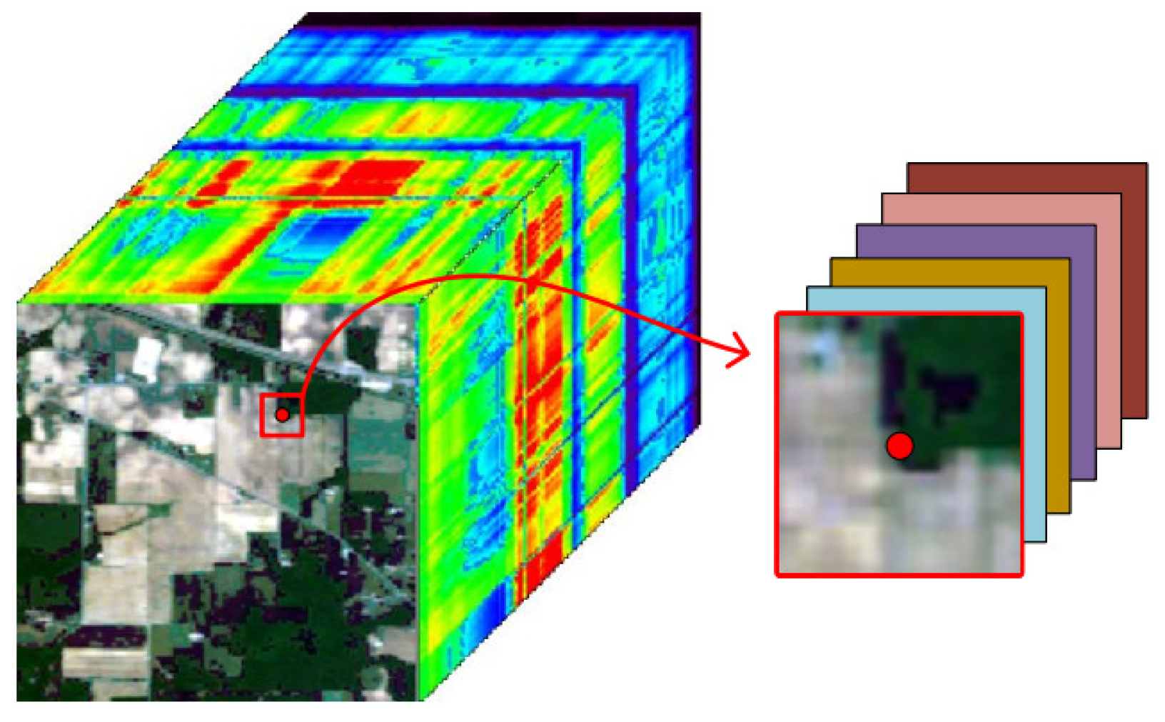
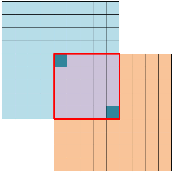
Despite these advances, most existing deep HSIC methods still adopt a patch-based input strategy. In this setting, each labeled pixel is taken as the patch center, and its surrounding neighborhood is extracted as the model input, as illustrated in Figure 1. This strategy is attractive because it enables the network to jointly exploit spectral and local spatial context. However, when training and test centers are randomly sampled from the same image, neighboring patches often overlap spatially. 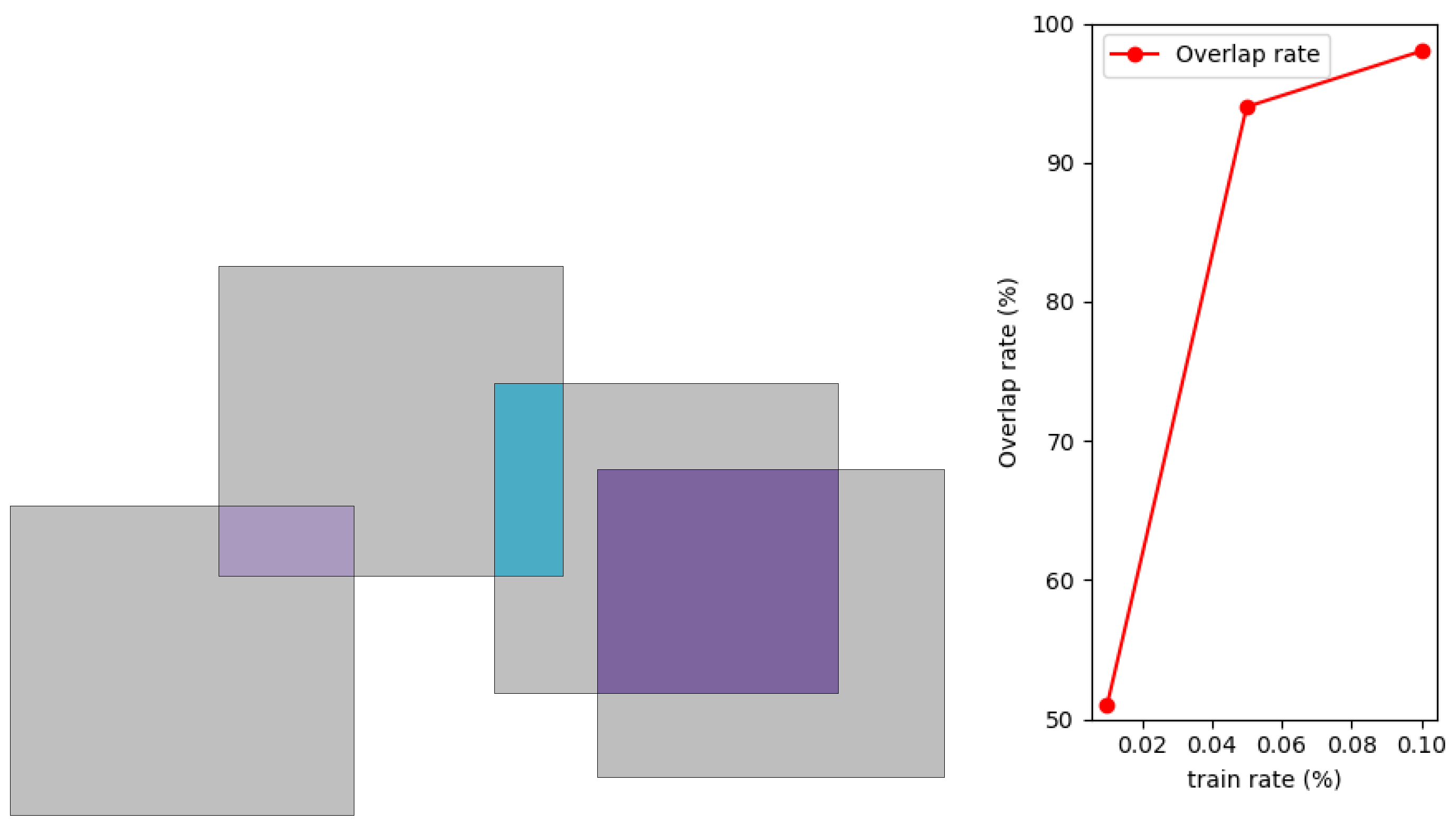As a result, non-central pixels from test samples may appear inside training patches, and vice versa, as illustrated in Figure 2 and Figure 3. This overlap introduces train–test leakage and can lead to overly optimistic evaluation results [31].

Recent studies have highlighted this problem in hyperspectral classification and suggested spatially disjoint or controlled sampling as a way to avoid overlap between training and test regions [32,33,34,35]. These strategies provide more reliable evaluation, but they may substantially reduce the number of available training samples, especially in small-sample settings. This limitation is particularly restrictive for HSIC, where labeled data are already scarce. Therefore, in addition to spatial separation, it is worthwhile to explore a complementary strategy that reduces overlap-induced leakage while preserving the conventional patch-based input format and retaining more training samples.

To this end, we propose a replacing overlapping pixels (ROP) strategy for patch-based HSIC. Instead of discarding spatial regions, ROP reconstructs patches by replacing overlapping pixels with same-class training pixels, thereby reducing direct train–test overlap at the pixel level. Since the reconstructed patches exhibit altered local spatial context, we further design a resolving data leakage network (RDLNet) equipped with a multiple feature extraction and fusion (MFEF) module. The proposed network combines multi-scale 3D and 1D convolutions to better capture complementary spectral–spatial information from ROP-reconstructed patches. The main contributions of this work are summarized as follows:

1.

We revisit the patch overlap problem in patch-based HSI classification and show that conventional random patch splitting may introduce train–test leakage, leading to overly optimistic performance estimates;

2.

We propose a replacement of overlapping pixels (ROP) strategy to construct a leakage-controlled patch evaluation strategy. ROP reduces direct overlap leakage while preserving the patch-based input format and retaining more samples than spatial buffer-based separation in small-sample settings;

3.

We design an RDLNet architecture with a multiple feature extraction and fusion (MFEF) module to model ROP-reconstructed patches more effectively. Experiments on five public datasets show that RDLNet achieves consistently strong performance under the proposed leakage-controlled strategy.

For ease of reference, a comprehensive list of abbreviations used throughout this manuscript is provided in

Table 1. List of abbreviations.

Abbreviation	Full Form
HSI	Hyperspectral Image
HSIc	Hyperspectral Image Classification
ROP	Replacing Overlapping Pixels
MFEF	Multiple Feature Extraction and Fusion
RDLNet	Resolving Data Leakage Network
CNN	Convolutional Neural Network
1DCNN	One-Dimensional Convolutional Neural Network
2DCNN	Two-Dimensional Convolutional Neural Network
3DCNN	Three-Dimensional Convolutional Neural Network
DL	Deep Learning
SVM	Support Vector Machine
RF	Random Forest
ViT	Vision Transformer
MCVT	Mixed Convolution Vision Transformer
DBDA	Double-Branch Dual-Attention
SSFTT	Spectral–Spatial Feature Tokenization Transformer
CMRCNN	Cross-Mixing Residual CNN
MIEPN	Multidimensional Information Expansion and Processing Network
PCA	Principal Component Analysis
OA	Overall Accuracy
AA	Average Accuracy
PU	Pavia University
SA	Salinas
SAR	Synthetic Aperture Radar
SOTA	State-of-the-Art

.

2. Materials and Methods

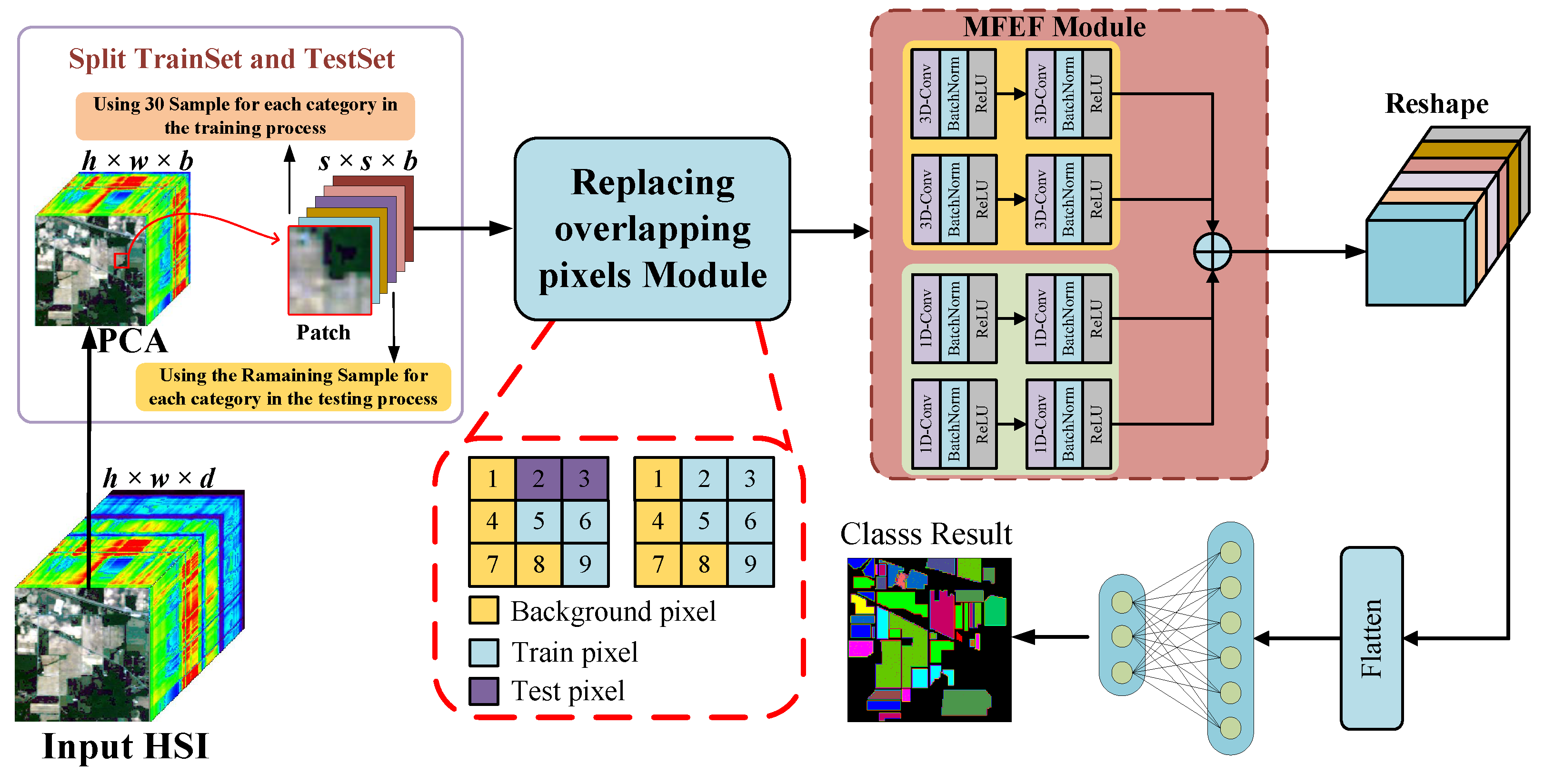
The proposed RDLNet, which mainly includes the ROP module and the MFEF module, is shown in Figure 4.

2.1. Resolving Data Leakage

In this paper, we mainly conduct a series of studies on the HSIc method based on patch data. Patch-based HSI classification usually takes each labeled pixel as the patch center and extracts its surrounding neighborhood as the model input. Under conventional random splitting, however, training and test centers are sampled from the same image, so their corresponding patches often overlap spatially. As a result, non-central pixels from the test set may appear inside training patches, and vice versa. This train–test overlap introduces data leakage and may lead to overly optimistic evaluation results. 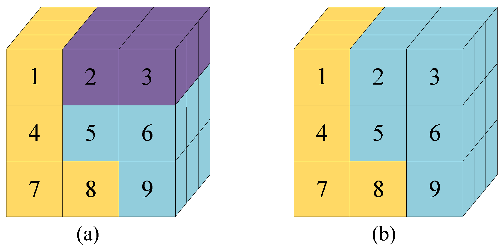Figure 5a illustrates this issue with a simplified $3\times 3$ example. Pixel 5 in the patch data is the pixel to be classified, pixels 2 and 9 belong to the pixels to be classified in the training set, and pixels 3 and 6 belong to the pixels to be classified in the test set. The remaining pixels 1, 4, 7, and 8 are all background pixels. This type of data partitioning leads to data leakage in the training process of the model, and the classification accuracy of the model increases as the patch size increases. This section explains how to solve the problem of data leakage as well as achieve good classification accuracy with less training data.

To solve the problem of the data leakage caused by pixel overlap between training and test data during the training process, we propose a method to replace overlapping pixels (ROP) in patch data and test pixels in the overlapping region of training patch data with training pixels of the same category. As shown in Figure 5b, pixel points 3 and 6 in the test set are to be classified, and these points are replaced by other pixels of the same category in the training set. Similarly, when constructing patches for test set pixels, if any position within a test patch contains a training pixel (i.e., a pixel that appears in the training set), that position is replaced by a randomly selected training pixel of the same class. Specifically, for each test patch centered at a test pixel, we scan all spatial positions within the patch window; if a position $(j,k)$ corresponds to a training pixel in the original image, we replace the spectral vector at that position with a randomly drawn spectral vector from the training set belonging to the same class label.

Algorithm 1 Replacing Overlapping Pixels Method

Input: $HSI\_Cubes\in {\mathbb{R}}^{N\times H\times W\times C}$, $SDL\in {\mathbb{R}}^{N\times H\times W}$, $OL\in {\mathbb{R}}^{N\times H\times W}$ Output: $HSI\_Cubes$ (with overlapping pixels replaced)   1: Initialize $ECC$ as an empty dictionary: $ECC\leftarrow \left\{\right\}$   2: $center\_row\leftarrow H/2$, $center\_col\leftarrow W/2$   3: for $i=0$ to $N-1$ do   4:    $class\_label\leftarrow SDL[i,center\_row,center\_col]$   5:    if $class\_label>0$ then   6:      $ECC[class\_label].\mathrm{append}(HSI\_Cubes[i,center\_row,center\_col,:\left]\right)$   7:    end if   8: end for   9: for $i=0$ to $N-1$ do 10:    for $j=0$ to $H-1$ do 11:      for $k=0$ to $W-1$ do 12:         if $SDL[i,j,k]==0$ and $OL[i,j,k]>0$ then 13:           $target\_class\leftarrow OL[i,j,k]$ 14:           $rand\_idx\leftarrow \mathrm{r}\mathrm{a}\mathrm{n}\mathrm{d}\mathrm{o}\mathrm{m}\_\mathrm{i}\mathrm{n}\mathrm{t}(0,|ECC[target\_class]|-1)$ 15:           $HSI\_Cubes[i,j,k,:]\leftarrow ECC[target\_class][rand\_idx]$ 16:         end if 17:      end for 18:    end for 19: end for 20: return  $HSI\_Cubes$

Therefore, the reconstructed patch should be understood as a leakage-controlled evaluation input rather than a natural spatial neighborhood sampled from the original scene.

The price of this strategy is that the natural spatial continuity of the patch is partially weakened, because some neighboring pixels are replaced by same-class pixels drawn from other spatial locations. Nevertheless, the patch-based input format is preserved, and the evaluation becomes less dependent on overlap-induced leakage. This produces a leakage-controlled setting for patch-based HSI classification.

The detailed mathematical formulations are given in Equations (1) and (2).

$$\begin{array}{cc}\hfill \mathit{HSI}\_{\mathit{Cubes}}_{i,j,k,:}& =\left\{\begin{array}{cc}\mathit{ECC}\left[{\mathit{OL}}_{i,j,k}\right][\mathit{rand}\_\mathit{idx}]\hfill & \mathrm{if}({\mathit{OL}}_{i,j,k}\ne 0)\mathrm{and}({\mathit{SDL}}_{i,j,k}=0)\hfill \\ \mathit{HSI}\_{\mathit{Cubes}}_{i,j,k,:}\hfill & \mathrm{otherwise}\hfill \end{array}\right.,\hfill \end{array}$$

(1)

$$\begin{array}{cc}\hfill \mathit{rand}\_\mathit{idx}& \sim \mathrm{Uniform}(0,|\mathit{ECC}\left[{\mathit{OL}}_{i,j,k}\right]|-1),\hfill \end{array}$$

(2)

where $\mathit{HSI}\_\mathit{Cubes}\in {\mathbb{R}}^{N\times H\times W\times C}$ represents the collection of all patch data, with N being the total number of patches, $H\times W$ the spatial dimensions of each patch, and C the number of spectral bands. The indices i, j, and k denote the patch index, row position within the patch, and column position within the patch, respectively. $\mathit{SDL}\in {\mathbb{R}}^{N\times H\times W}$ is the label map indicating which pixels belong to the training set (non-zero values correspond to training pixels, zero values indicate test or background pixels). $\mathit{OL}\in {\mathbb{R}}^{N\times H\times W}$ is the original ground-truth label map for all pixels in the image. $\mathit{ECC}$ is a class-wise dictionary structure where $\mathit{ECC}\left[c\right]$ is a list storing all training pixel spectral vectors belonging to class c. Specifically, $\mathit{ECC}\left[c\right]=\{{\mathbf{x}}_1^{\left(c\right)},{\mathbf{x}}_2^{\left(c\right)},\dots ,{\mathbf{x}}_{n_c}^{\left(c\right)}\}$, where $n_c$ is the number of training samples in class c and each ${\mathbf{x}}_t^{\left(c\right)}\in {\mathbb{R}}^C$ is a spectral vector. The variable $\mathit{rand}\_\mathit{idx}$ is a random integer uniformly sampled from $[0,n_c-1]$, ensuring that each replacement draws a different training sample from the same class.

Algorithm 1 summarizes the implementation of ROP. First, a class-wise candidate pool is built from the center pixels of the training patches. Then, each patch is scanned position by position, and every overlapping non-central pixel is replaced according to Equations (1) and (2). Since only overlapping positions are modified, the total number of training and test patches remains unchanged.

In ROP, the replacement pixel at each overlapping position is randomly sampled from the class-wise candidate pool. Therefore, the reconstructed patch is not unique, and different random seeds may lead to slightly different local spectral–spatial configurations and, consequently, slightly different classification results. This stochastic effect is expected to be more noticeable when the candidate pool of a class is small or when the class exhibits strong intra-class variability.

2.2. Multiple Feature Extraction and Fusion Module

After applying the ROP strategy, the reconstructed patches retain class-relevant spectral information but exhibit partially modified local spatial context. To better model such inputs, we design a multiple feature extraction and fusion (MFEF) module. The purpose of MFEF is to extract complementary spectral–spatial representations at different scales and then fuse them for final classification.

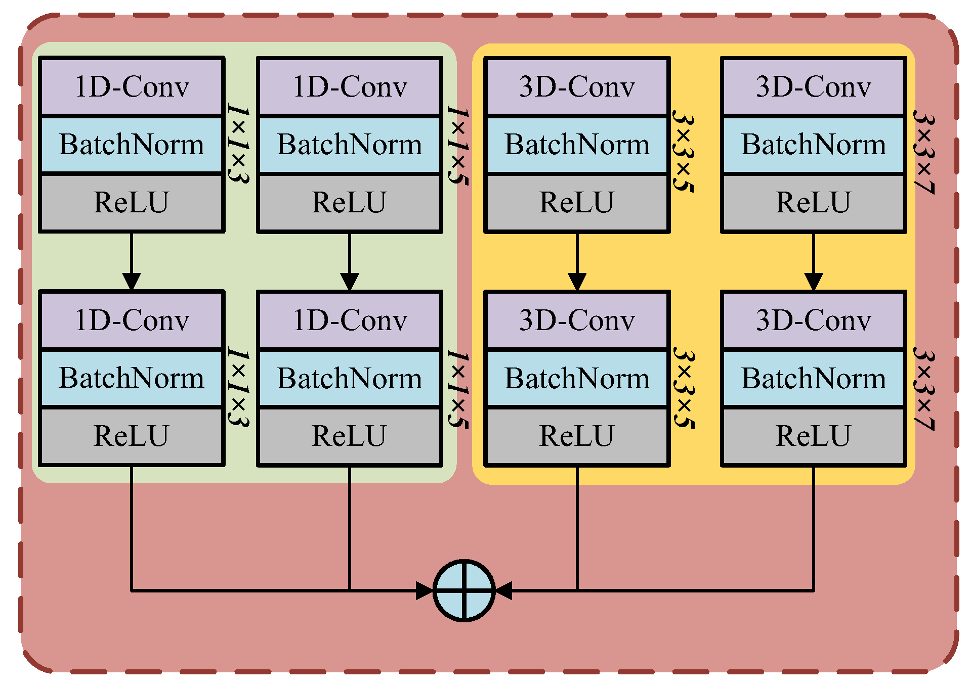
As shown in Figure 6, the MFEF module consists of two parallel 3D convolution branches and one parallel 1D convolution branch. The two 3D branches are used to capture joint spectral–spatial features under different spectral receptive fields, while the 1D branch focuses on fine-grained spectral dependency modeling. In this way, the module combines local spectral–spatial context with detailed spectral discrimination, which is particularly useful for ROP-reconstructed patches whose spatial continuity is partially weakened.

More specifically, the 3D branches operate on the input patch cube and learn spatial–spectral representations from different kernel depths, enabling the network to capture multi-scale contextual information. The 1D branch models spectral correlations along the band dimension and provides complementary spectral cues that are less sensitive to spatial perturbation. The outputs of the three branches are then fused and fed into the classifier to obtain the final category prediction.

The 3D and 1D convolution operations used in the network are defined as follows:

$$\begin{array}{cc}\hfill f_{i,j}^{x,y,z}& =\mathrm{\Phi }\left(\sum _m\sum _{p=0}^{P_i-1}\sum _{q=0}^{Q_i-1}\sum _{r=0}^{R_i-1}{\omega }_{i,j,m}^{p,q,r}{f}_{(i-1)m}^{(x+p)(y+q)(z+r)}+b_{i,j}\right),\hfill \\ \hfill f_{i,j}^x& =\mathrm{\Phi }\left(\sum _m\sum _{p=0}^{P_i-1}{\omega }_{i,j,m}^p{f}_{(i-1)m}^{(x+p)}+b_{i,j}\right),\hfill \end{array}$$

(3)

Here, $f_{i,j}^{x,y,z}$ denotes the output at spatial–spectral position $(x,y,z)$ in the jth feature map of the ith 3D convolution layer, and $f_{i,j}^x$ denotes the output at position x in the jth feature map of the ith 1D convolution layer. $\mathrm{\Phi }(·)$ is the activation function, $\omega$ represents the convolution kernel weights, and $b_{i,j}$ is the bias term.

By combining multi-scale 3D feature extraction with 1D spectral modeling, MFEF provides a compact and effective representation for HSI classification under the proposed leakage-controlled setting.

3. Experiments and Results

3.1. Datasets and Experimental Setup

In order to ascertain the viability of the proposed model, five datasets were selected for experimental analysis: Pavia University (PU), Salinas (SA), Xuzhou [36,37], Honghu [38], and Longkou [39]. The image specifications of the PU dataset are 610*340*102, and the ROSIS sensor is used to shoot over Pavia, northern Italy, with a ground truth of nine classes. The image specifications of the SA dataset are 512*217*204, obtained by the AVIRIS sensor, and the image ground truth is 16 classes. The image size of the Xuzhou dataset is 500*260*436, and the HYSPEX hyperspectral airborne camera (Norsk Elektro Optikk AS, Skedsmokorset, Norway) is used to shoot over the suburban sites of Xuzhou. Its ground truth is nine classes. The image specifications of the Honghu dataset are 940*475*270, obtained by the Headwall Nano-Hyperspec sensor, including 22 classes. The image specifications of the Longkou dataset with the Headwall Nano-Hyperspec sensor are 550*400*270, wherein 9 classes are present.

Table 2. Numbers of training samples for the first three dataset.

	Honghu		Salinas		Pavia University
ID	Class Name	Samples	Class Name	Samples	Class Name	Samples
1	Red roof	30	Brocoli green weeds 1	30	Asphalt	30
2	Road	30	Brocoli green weeds 2	30	Meadows	30
3	Bare soil	30	Fallow	30	Gravel	30
4	Cotton	30	Fallow rough plow	30	Trees	30
5	Cotton firewood	30	Fallow smooth	30	Painted metal sheets	30
6	Rape	30	Stubble	30	Bare Soil	30
7	Chinese cabbage	30	Celery	30	Bitumen	30
8	Pakchoi	30	Grapes untrained	30	Self-Blocking Bricks	30
9	Cabbage	30	Soil vinyard develop	30	Shadows	30
10	Tuber mustard	30	Corn senesced green weeds	30		30
11	Brassica parachinensis	30	Lettuce romaine 4 wk	30		30
12	Brassica chinensis	30	Lettuce romaine 5 wk	30
13	Small Brassica chinensis	30	Lettuce romaine 6 wk	30
14	Lactuca sativa	30	Lettuce romaine 7 wk	30
15	Celtuce	30	Vinyard untrained	30
16	Film covered lettuce	30	Vinyard vertical trellis	30
17	Romaine lettuce	30
18	Carrot	30
19	White radish	30
20	Garlic sprout	30
21	Broad bean	30
22	Tree	30

and

Table 3. Number of training samples for the latter two datasets.

	Longkou		Xuzhou
ID	Class Name	Samples	Class Name	Samples
1	Corn	30	Bareland1	30
2	Cotton	30	Lakes	30
3	Sesame	30	Coals	30
4	Broad-leaf soybean	30	Cement	30
5	Narrow-leaf soybean	30	Crops-1	30
6	Rice	30	Trees	30
7	Water	30	Bareland2	30
8	Roads and houses	30	Crops	30
9	Mixed weed	30	Red-title	30

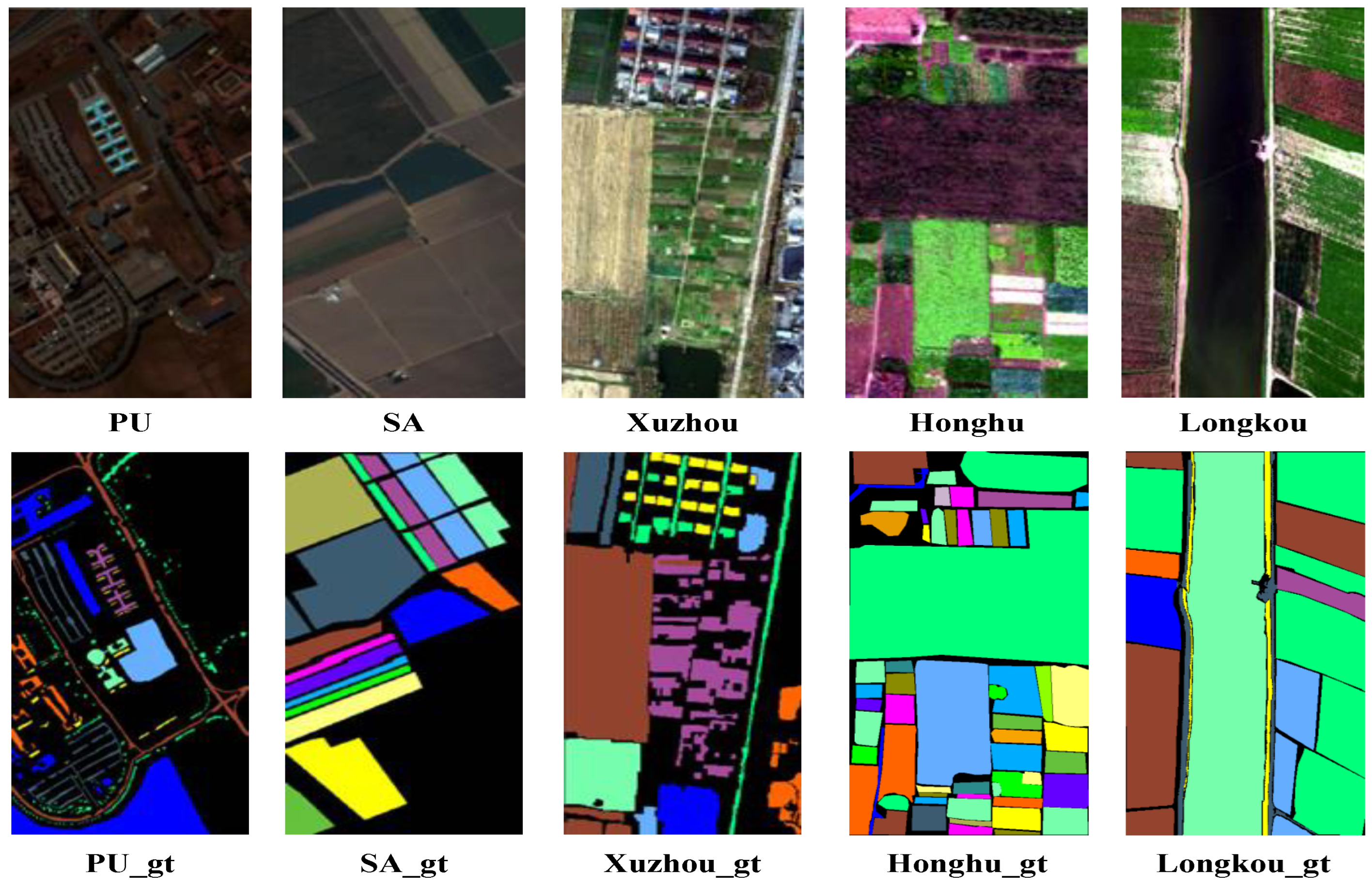
show the number of training samples of each class for these five datasets. Figure 7 shows their corresponding false color images and ground truth maps.

It should be stressed that, as the operation PCA (principal component analysis) has been demonstrated to be useful for HSIc [40], we here also adopt it in RDLNet. For the principal component values of PCA, the starting point is [20; 30; 40; 50]. The number of training individuals for each category of these datasets was set to 30.

Table 4. OA (%) under different PCA dimensions. The best dataset results under the different principal component values are highlighted in bold.

	PCA	20	30	40	50
Datasets
PU		77.88	82.97	76.64	71.55
SA		90.51	93.07	94.92	94.66
Xuzhou		94.42	89.87	91.34	92.36
Honghu		73.94	70.62	75.86	73.05
Longkou		92.62	95.22	92.80	89.33

illustrates the OA values for varying principal component values. It can be observed that the Xuzhou dataset exhibits the best results when the value of the principal component is set to 20. Similarly, the PU and Longkou datasets demonstrate the best results when the value of the principal component is set to 30. When the value is set to 40, the SA and Honghu datasets yield the best results. Therefore, the value of PCA for these five datasets was set to [30; 40; 20; 40; 30].To ensure a fair comparison, the same PCA configuration was applied uniformly to all comparative methods. This controlled setting avoids method-specific PCA tuning and makes the comparison focus on architectural differences.

In addition to reducing the dimensionality of these datasets, other parameter values are also set. During the training process, the patch size, learning rate, and training period were set to 11, 0.0001, and 100, respectively. Due to the high cost of labelling hyperspectral images, a total of 30 randomly selected center pixels were chosen for each category as the training set in these datasets. Each center pixel was then expanded into an $11\times 11\times C$ patch, where C denotes the number of spectral bands after PCA. Therefore, the total number of training patches equals $30\times N_{\mathrm{classes}}$, and applying ROP changes only the spectral content of overlapping positions without changing the number of training or test patches.

To demonstrate the effectiveness of this network, nine methods are selected for a fair comparison. They are 1DCNN [12], 2DCNN [13], 3DCNN [16], ViT [22], MCVT [41], DBDA [42], SSFTT [25], CMRCNN [43], and MIEPN [44]. Note that the aforementioned methods are compared with the method used in this work, both without and with the ROP strategy. To ensure statistical reliability and account for the variability introduced by random sampling in the ROP procedure, all experiments are repeated five times with different random seeds (seeds = 0, 1, 2, 3, 4). Each run involves independent data splitting, ROP reconstruction, and model training. The reported results in

Table 5. Classification results (%) with 30 training samples per class under the conventional patch strategy. The best results are highlighted in bold.

		1D-CNN	2D-CNN	3D-CNN	ViT	MCVT	DBDA	SSFTT	CMRCNN	MIEPN
	OA	65.17 ± 2.14	89.25 ± 2.53	89.41 ± 2.63	82.98 ± 3.49	91.68 ± 3.28	92.51 ± 1.84	90.28 ± 4.96	93.36 ± 1.56	90.45 ± 0.93
PU	AA	73.26 ± 1.82	91.70 ± 0.87	91.67 ± 1.19	86.62 ± 2.72	93.43 ± 1.64	93.94 ± 1.30	92.81 ± 1.32	94.21 ± 1.30	92.03 ± 0.94
	Kappa	56.33 ± 2.79	86.02 ± 3.13	86.21 ± 3.32	78.07 ± 4.39	89.17 ± 4.16	90.17 ± 2.40	87.47 ± 6.01	91.28 ± 2.04	87.51 ± 1.19
	OA	87.75 ± 0.66	96.08 ± 0.50	95.24 ± 0.23	94.67 ± 0.46	95.94 ± 0.50	95.45 ± 0.58	96.21 ± 0.27	96.52 ± 1.18	96.30 ± 0.57
SA	AA	93.73 ± 0.37	98.21 ± 0.33	97.94 ± 0.16	97.72 ± 0.29	98.21 ± 0.33	98.10 ± 0.12	98.38 ± 0.17	98.31 ± 0.82	98.35 ± 0.31
	Kappa	86.39 ± 0.72	95.64 ± 0.56	94.70 ± 0.25	94.07 ± 0.52	95.48 ± 0.55	94.94 ± 0.64	95.79 ± 0.30	96.13 ± 1.30	95.87 ± 0.64
	OA	78.62 ± 0.88	93.64 ± 1.04	95.53 ± 0.57	94.64 ± 1.04	94.83 ± 0.90	95.39 ± 0.55	94.40 ± 1.53	95.69 ± 0.69	93.96 ± 2.02
Xuzhou	AA	82.64 ± 0.84	95.86 ± 0.65	97.00 ± 0.44	95.97 ± 0.81	96.74 ± 1.14	97.09 ± 0.45	96.52 ± 0.52	97.39 ± 0.57	95.50 ± 2.31
	Kappa	73.53 ± 1.01	92.00 ± 1.34	94.36 ± 0.72	93.25 ± 1.31	93.49 ± 1.13	94.19 ± 0.69	92.97 ± 1.89	94.56 ± 0.86	92.37 ± 2.59
	OA	50.58 ± 1.09	84.77 ± 1.35	86.29 ± 1.00	78.62 ± 3.72	87.96 ± 1.64	82.05 ± 1.98	82.82 ± 1.52	89.71 ± 1.04	86.38 ± 1.36
Honghu	AA	48.32 ± 0.38	87.10 ± 0.96	86.84 ± 0.83	75.32 ± 4.81	89.38 ± 1.30	82.93 ± 0.82	85.59 ± 1.81	90.75 ± 0.84	87.74 ± 0.97
	Kappa	43.87 ± 1.11	81.33 ± 1.50	83.06 ± 1.16	73.96 ± 4.26	85.10 ± 1.96	78.10 ± 2.22	79.06 ± 1.78	87.20 ± 1.25	83.20 ± 1.59
	OA	85.74 ± 1.80	95.18 ± 2.13	95.73 ± 0.64	94.03 ± 1.63	95.96 ± 1.70	97.54 ± 0.92	95.02 ± 2.10	95.77 ± 0.64	96.01 ± 1.20
Longkou	AA	84.54 ± 1.05	95.60 ± 1.33	96.06 ± 0.30	93.30 ± 1.06	96.38 ± 1.21	97.88 ± 0.41	95.42 ± 1.14	96.33 ± 0.20	96.83 ± 0.52
	Kappa	81.87 ± 2.21	93.77 ± 2.71	94.46 ± 0.81	92.28 ± 2.06	94.76 ± 2.16	96.79 ± 1.19	93.56 ± 2.66	94.51 ± 0.82	94.82 ± 1.55

and

Table 6. Classification results (%) with 30 training samples per class under the proposed ROP strategy. The best results are highlighted in bold.

		1D-CNN	2D-CNN	3D-CNN	ViT	MCVT	DBDA	SSFTT	CMRCNN	MIEPN	RDLNet
	OA	65.17 ± 2.14	70.85 ± 2.64	75.85 ± 0.81	69.41 ± 10.60	75.24 ± 3.01	72.88 ± 2.35	72.39 ± 5.14	74.15 ± 2.68	71.69 ± 5.59	82.29 ± 2.35
PU	AA	73.26 ± 1.82	79.14 ± 0.64	83.11 ± 1.44	82.42 ± 1.56	82.31 ± 2.11	82.88 ± 1.14	80.49 ± 3.81	83.56 ± 1.18	81.14 ± 2.16	89.22 ± 1.65
	Kappa	56.33 ± 2.79	63.13 ± 2.58	69.25 ± 0.84	62.62 ± 10.28	68.39 ± 3.58	67.58 ± 2.90	65.04 ± 6.14	67.56 ± 2.90	64.71 ± 5.92	77.32 ± 2.84
	OA	87.75 ± 0.66	90.27 ± 1.61	91.85 ± 0.78	91.56 ± 1.10	90.68 ± 1.59	91.71 ± 0.65	91.43 ± 1.22	90.09 ± 3.29	91.35 ± 1.52	92.80 ± 2.22
SA	AA	93.73 ± 0.37	94.26 ± 1.10	95.75 ± 0.76	94.94 ± 1.25	94.83 ± 1.44	94.98 ± 0.49	95.33 ± 1.31	93.37 ± 3.28	95.74 ± 0.84	96.53 ± 2.32
	Kappa	86.39 ± 0.72	89.18 ± 1.83	90.92 ± 0.87	90.61 ± 1.22	89.63 ± 1.76	89.88 ± 0.73	90.46 ± 1.38	88.99 ± 3.63	91.47 ± 1.71	91.97 ± 2.49
	OA	78.62 ± 0.88	82.50 ± 3.16	89.27 ± 1.06	82.97 ± 2.26	80.00 ± 7.49	88.23 ± 1.25	78.28 ± 10.39	82.53 ± 6.52	81.58 ± 2.84	91.54 ± 1.06
Xuzhou	AA	82.64 ± 0.84	87.77 ± 2.63	92.12 ± 0.77	86.73 ± 3.53	82.02 ± 10.15	93.03 ± 1.10	84.63 ± 3.81	89.63 ± 2.70	86.73 ± 1.84	95.00 ± 0.51
	Kappa	73.53 ± 1.01	78.53 ± 3.77	86.59 ± 1.35	78.62 ± 2.95	75.40 ± 8.87	85.04 ± 1.54	73.69 ± 11.60	78.74 ± 7.46	77.20 ± 3.27	89.42 ± 1.31
	OA	50.58 ± 1.09	59.97 ± 3.33	62.90 ± 3.01	67.99 ± 3.36	62.99 ± 4.07	52.13 ± 2.99	54.82 ± 12.05	50.01 ± 14.07	67.43 ± 3.75	70.52 ± 1.57
Honghu	AA	48.32 ± 0.38	60.82 ± 4.36	63.15 ± 2.16	67.09 ± 1.37	64.63 ± 0.73	65.21 ± 1.71	58.67 ± 6.06	56.92 ± 9.33	65.50 ± 2.63	68.59 ± 2.09
	Kappa	43.87 ± 1.11	53.55 ± 3.67	56.66 ± 3.21	64.62 ± 3.51	56.75 ± 3.80	51.31 ± 2.96	49.10 ± 10.72	44.71 ± 12.52	61.29 ± 4.00	62.15 ± 1.51
	OA	85.74 ± 1.80	67.27 ± 6.85	78.98 ± 3.10	79.00 ± 4.14	76.78 ± 5.91	86.90 ± 2.51	73.04 ± 4.18	72.76 ± 6.22	77.14 ± 2.90	90.82 ± 3.33
Longkou	AA	84.54 ± 1.05	77.40 ± 2.64	83.73 ± 1.32	81.53 ± 3.82	84.18 ± 3.10	89.19 ± 1.41	77.61 ± 5.60	81.98 ± 2.50	82.76 ± 2.54	92.54 ± 2.55
	Kappa	81.87 ± 2.21	61.00 ± 7.05	74.02 ± 3.58	73.66 ± 4.98	71.60 ± 6.63	83.13 ± 3.14	67.02 ± 4.80	67.04 ± 6.89	71.70 ± 3.37	88.28 ± 4.14

are presented as “mean ± standard” deviation across these five runs. To evaluate the performance of various methods, the following metrics were employed: Overall Accuracy (OA), Average Accuracy (AA), and Kappa Coefficient (Kappa), that is,

$$\mathrm{OA}={\displaystyle \frac{{\sum }_{i=1}^{\mathrm{Num}}{C}_{ii}}{{\mathrm{TNum}}_{\mathrm{test}}}}.$$

(4)

$$\mathrm{AA}={\displaystyle \frac{{\sum }_{i=1}^{\mathrm{Num}}\frac{C_{ii}}{N_i}}{\mathrm{Num}}}.$$

(5)

$$\mathrm{Kappa}={\displaystyle \frac{\mathrm{OA}-{\sum }_{i=1}^{\mathrm{Num}}\left(\frac{{\mathrm{H}}_i}{{\mathrm{TNum}}_{\mathrm{test}}}·\frac{{\mathrm{L}}_i}{{\mathrm{TNum}}_{\mathrm{test}}}\right)}{1-{\sum }_{i=1}^{\mathrm{Num}}\left(\frac{{\mathrm{H}}_i}{{\mathrm{TNum}}_{\mathrm{test}}}·\frac{{\mathrm{L}}_i}{{\mathrm{TNum}}_{\mathrm{test}}}\right)}}.$$

(6)

where $Num$ denotes the number of classes, $C_{ii}$ is the number of correctly classified samples in class i, $TNu{m}_{\mathrm{test}}$ is the total number of test samples, and $N_i$ is the number of test samples in class i. In Equation (6), $H_i$ and $L_i$ denote the sums of the ith row and the ith column of the confusion matrix, respectively.

3.2. Results and Analyses

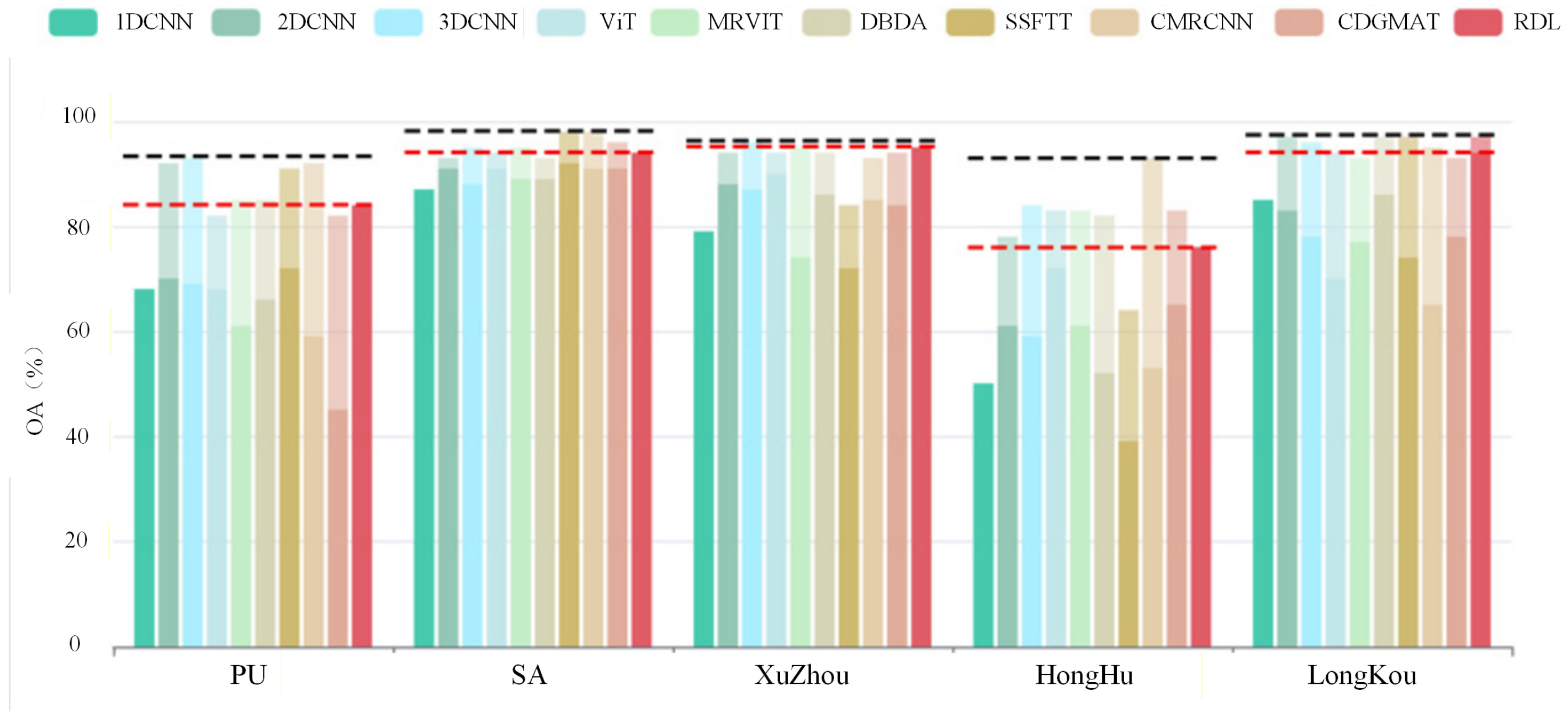
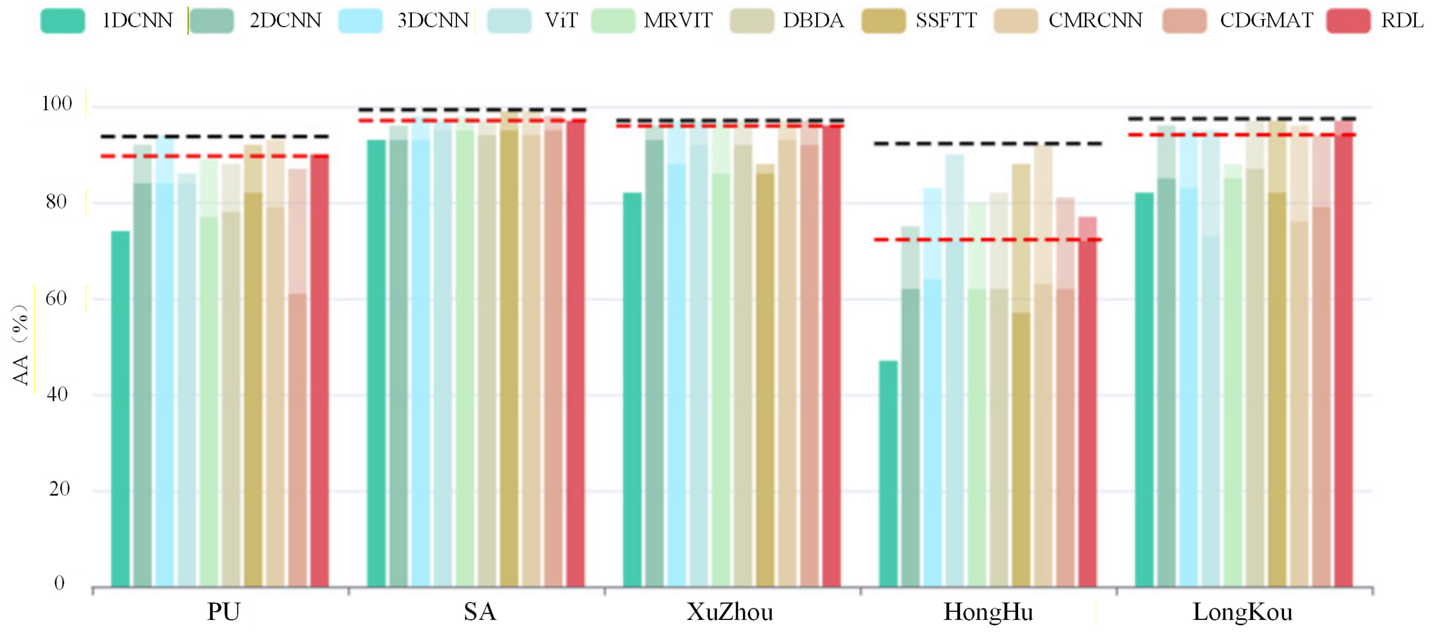
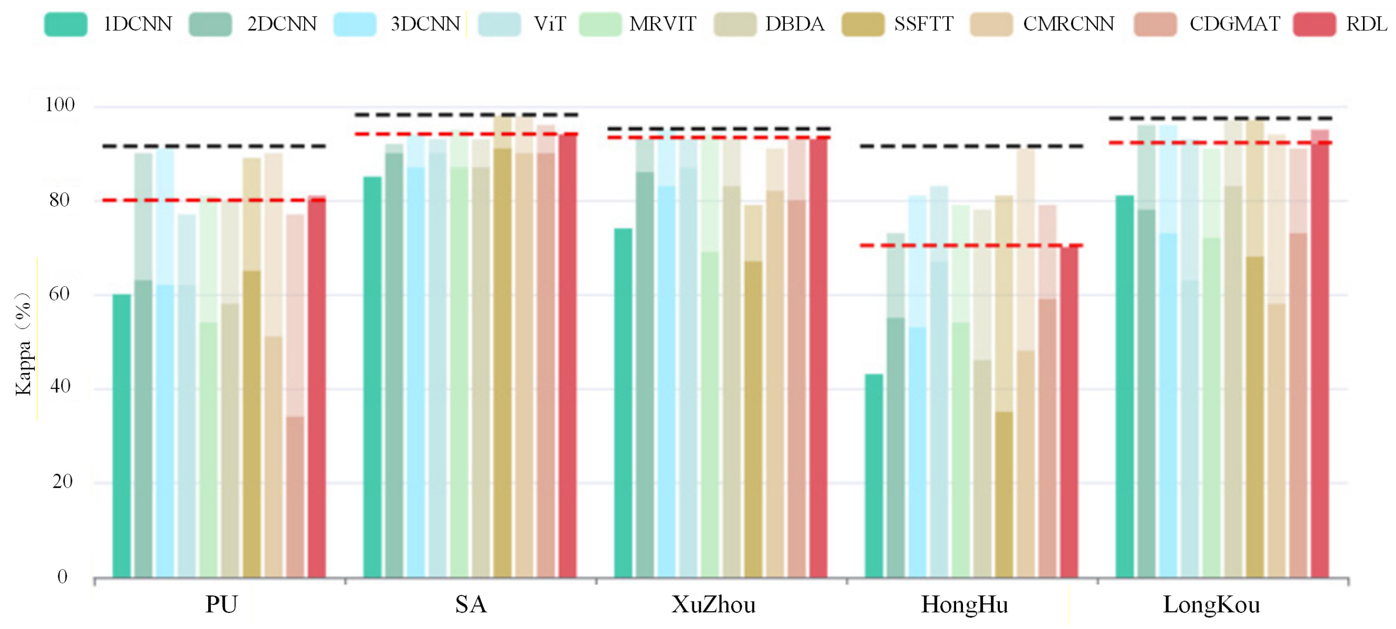
Figure 8, Figure 9 and Figure 10 summarize the performance of all methods across the five datasets. In each bar chart, the darker bottom portion represents the robust classification performance obtained under the proposed leakage-controlled ROP strategy. The lighter, transparent portion on top explicitly highlights the performance gap—specifically, the inflated accuracy caused by overlap-induced data leakage under the conventional patch strategy. This visual comparison provides a direct and stark view of how severely train–test overlap can overestimate a model’s true generalization capability. As shown in these figures, while baseline methods experience a dramatic collapse in accuracy once the leaked information is removed, RDLNet (indicated by the red dashed line) effectively defends against this degradation.

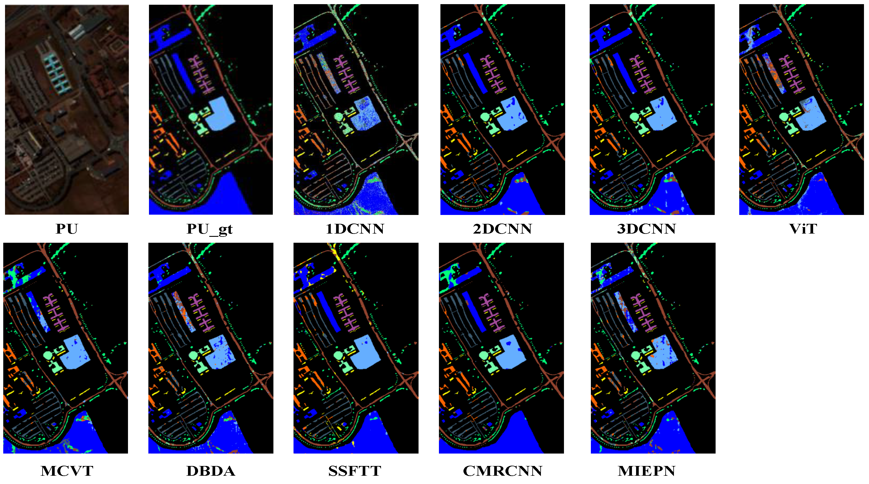
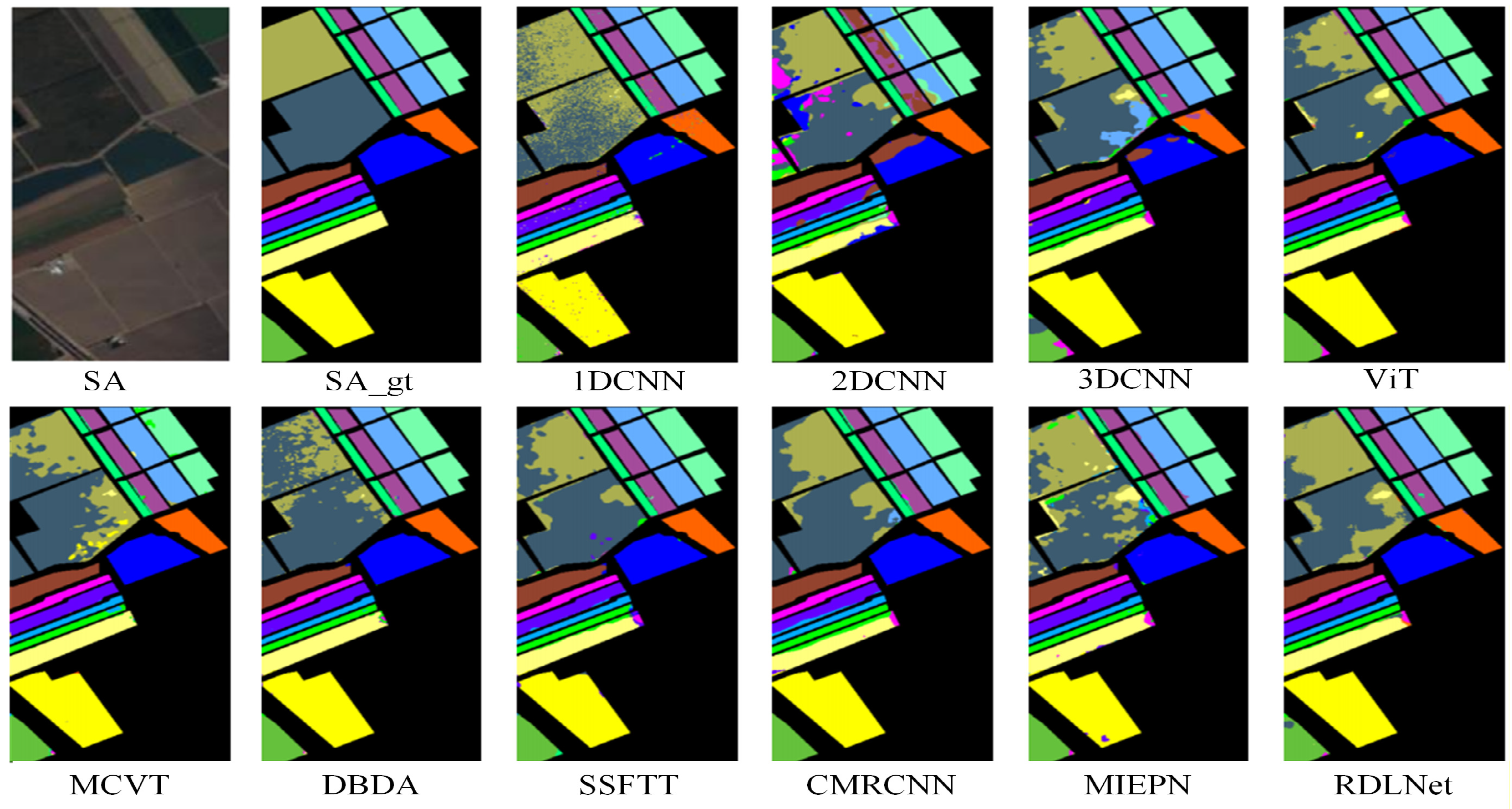
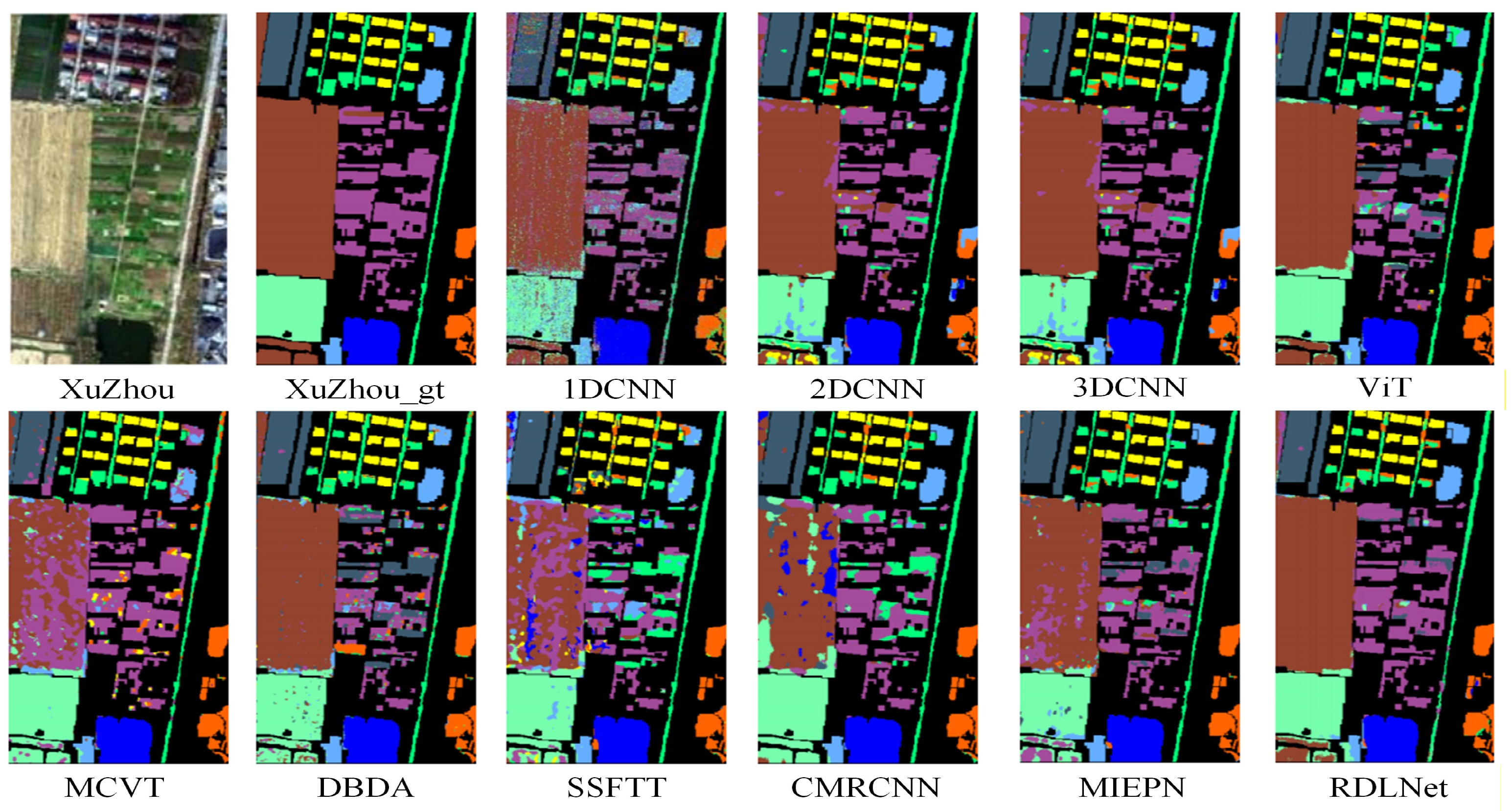
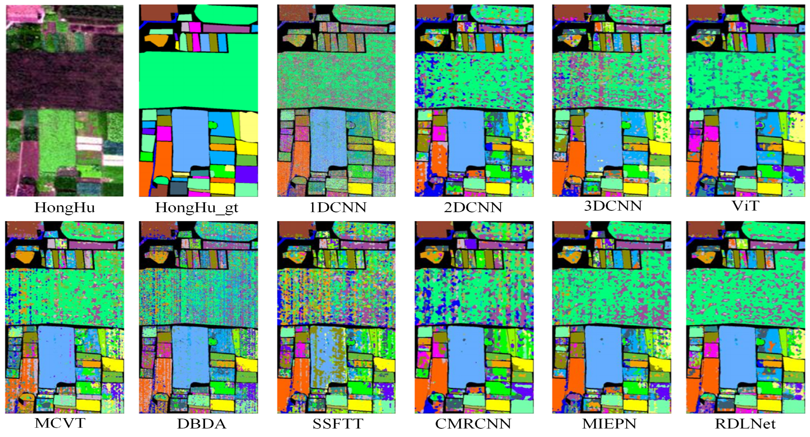
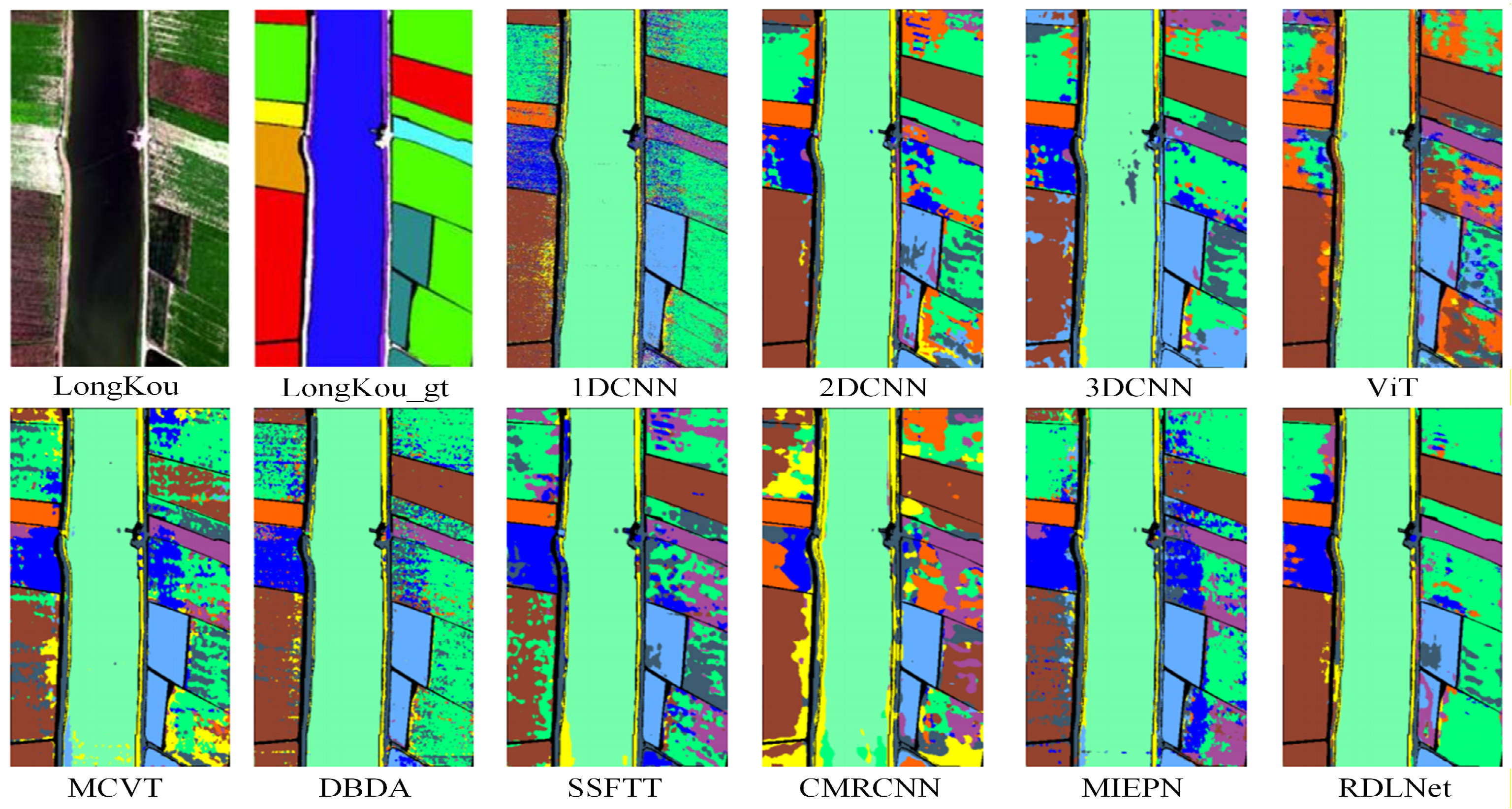
Table 5 reports the results obtained under the conventional random patch strategy. Since this strategy suffers from overlap-induced train–test leakage, these results are presented only for reference. As shown in the table, many methods achieve very high accuracies under this setting, such as CMRCNN on PU and DBDA on LongKou. However, these results may be inflated because overlapping pixels allow the model to benefit from leaked information. The classification maps in Figure 11 further illustrate this phenomenon.

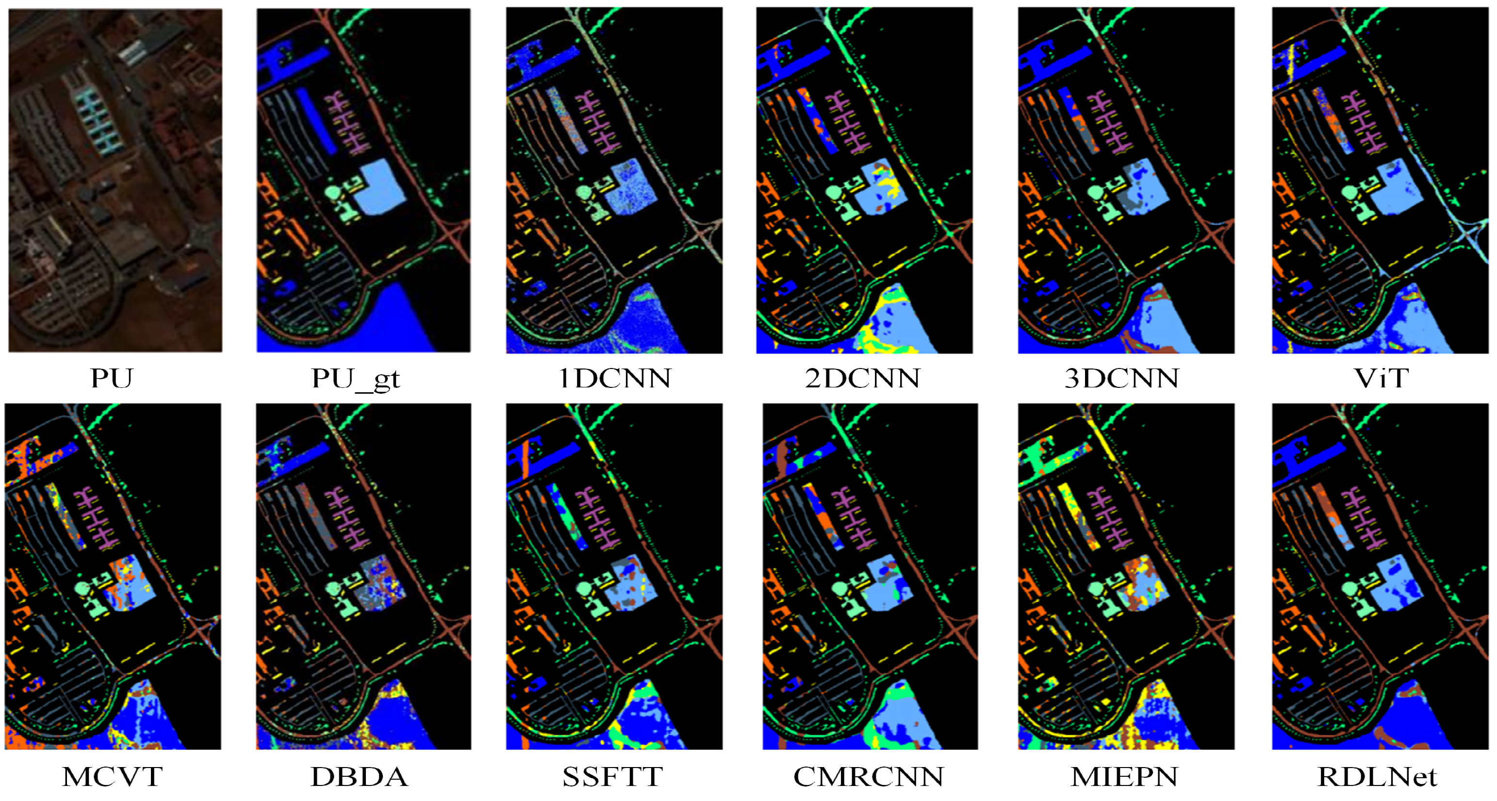
Table 6 and Figure 12, Figure 13, Figure 14, Figure 15 and Figure 16 present the main results under the proposed leakage-controlled strategy. After applying ROP, the performance of most comparative methods drops substantially, indicating that part of their apparent gains under the conventional strategy comes from overlap-induced leakage rather than true generalization. For example, the OA of CMRCNN on PU decreases from 93.36 (±1.56)% to 74.15 (±2.68)%, and SSFTT on Longkou decreases from 95.02 (±2.10)% to 73.04 (±4.18)%.

In contrast, RDLNet consistently achieves the best performance on all five datasets under the ROP-based setting. Specifically, it obtains OA values of 82.29 (±2.35)% on PU, 92.80 (±2.22)% on SA, 91.54 (±1.06)% on Xuzhou, 67.99 (±1.57)% on Honghu, and 89.90 (±3.33)% on Longkou. Compared with the second-best method, RDLNet improves mean OA by 6.44% on PU, 0.95% on SA, 2.27% on Xuzhou, 2.53% on Honghu, and 3.92% on Longkou. These results indicate that the proposed MFEF design is more effective for modeling ROP-reconstructed patches.

Beyond the average results, the standard deviations in Table 5 and Table 6 quantify the run-to-run variability caused by random data splitting, stochastic ROP reconstruction, and network optimization. In general, a smaller standard deviation indicates that a method is less sensitive to random factors and yields more repeatable performance, whereas a larger deviation suggests that the reported accuracy depends more strongly on specific random realizations. Under the proposed ROP setting, several baseline methods exhibit relatively large fluctuations on some datasets, such as ViT on PU (OA: 69.41 ± 10.60), SSFTT on Xuzhou (OA: 78.28 ± 10.39), and CMRCNN on Honghu (OA: 50.01 ± 14.07), indicating limited stability once overlap-induced leakage is removed. In contrast, RDLNet maintains moderate deviations across the five datasets (OA std: ±2.35 on PU, ±2.22 on SA, ±1.06 on Xuzhou, ±1.57 on Honghu, and ±3.33 on Longkou), which suggests that its performance advantage is not due to a favorable single run but can be reproduced under different random seeds.

The advantage of RDLNet is also reflected in AA and Kappa. On PU, for example, RDLNet achieves 90.48% AA and 80.00% Kappa, both clearly higher than those of the compared methods. Similar trends can be observed on the other four datasets. This suggests that the proposed model not only improves overall classification accuracy but also maintains more balanced class-wise performance under the leakage-controlled setting.

Overall, the results support two conclusions. First, conventional random patch splitting may considerably overestimate the performance of HSI classifiers because of train–test overlap. Second, once this overlap is controlled, RDLNet remains consistently strong across datasets, showing that the proposed architecture is better suited to fair patch-based HSI evaluation.

3.3. Ablation Study

To better understand the contribution of each component in the proposed model, we conduct ablation experiments on the PU dataset under the ROP-based setting.

Table 7. Ablation results (%) of different branch combinations in rdlnet on the PU dataset under the ROP strategy. The symbol “✓” indicates that the corresponding branch is enabled, while “×” indicates that it is disabled. The best results are highlighted in bold.

3D	2D	1D	OA	AA	Kappa
✓	×	×	81.55	88.67	76.22
×	✓	×	81.77	89.17	76.62
×	×	✓	82.54	88.57	77.21
✓	✓	×	83.60	89.87	78.74
✓	×	✓	84.56	90.48	80.00
×	✓	✓	82.20	89.19	76.97
✓	✓	✓	80.35	87.00	74.49

reports the results of different branch combinations in the MFEF module.

Using a single branch already yields competitive performance, with the 1D branch achieving the best OA among the three single-branch variants. However, combining two branches consistently improves the results, which indicates that feature representations from different dimensions are complementary. Among all combinations, the 3D + 1D setting achieves the best performance, reaching 84.56% OA, 90.48% AA, and 80.00% Kappa. This confirms that the proposed MFEF design effectively combines joint spectral–spatial modeling with fine-grained spectral discrimination.

In contrast, the simultaneous use of 3D, 2D, and 1D branches leads to a noticeable performance drop. A likely reason is that the additional 2D branch introduces redundant or less compatible spatial features after ROP modifies the local neighborhood structure. At the same time, the three-branch configuration increases optimization difficulty in the small-sample setting, which may further weaken the effectiveness of feature fusion. Therefore, the best performance is obtained not by using all possible branches, but by combining the most complementary ones.

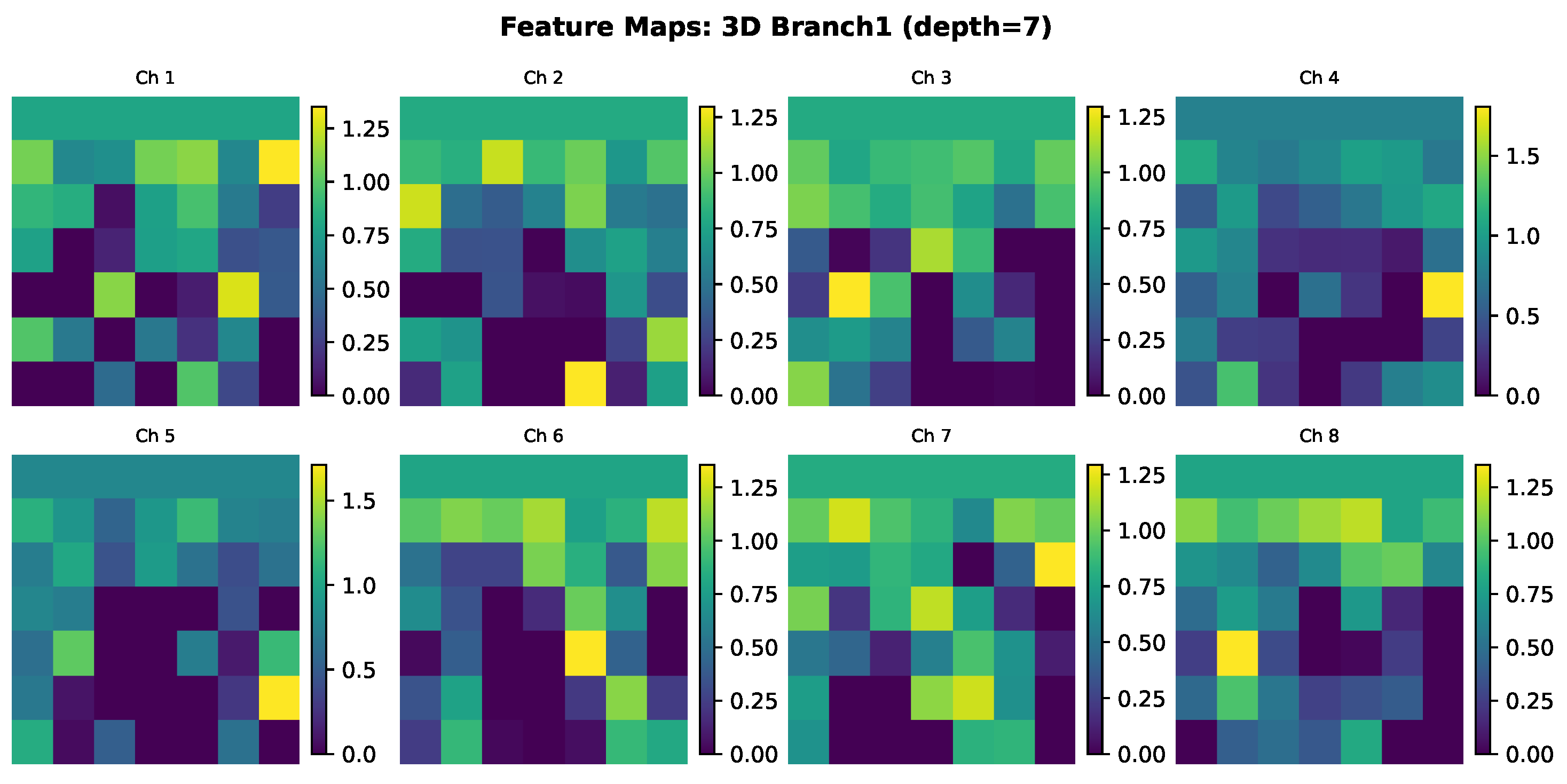
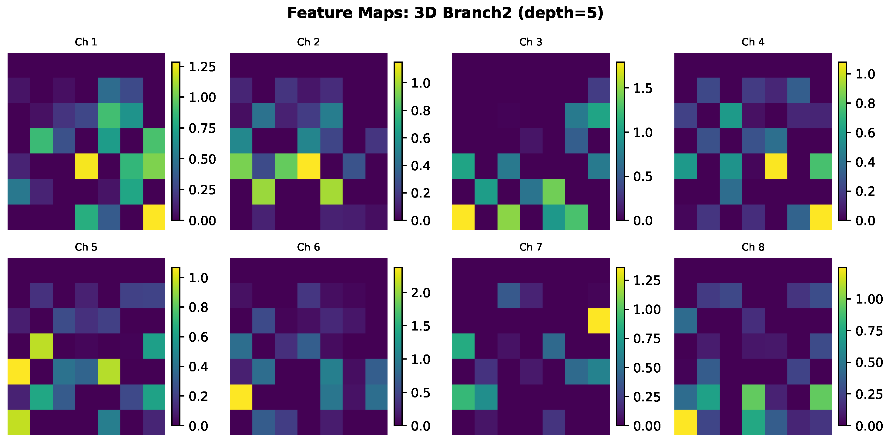
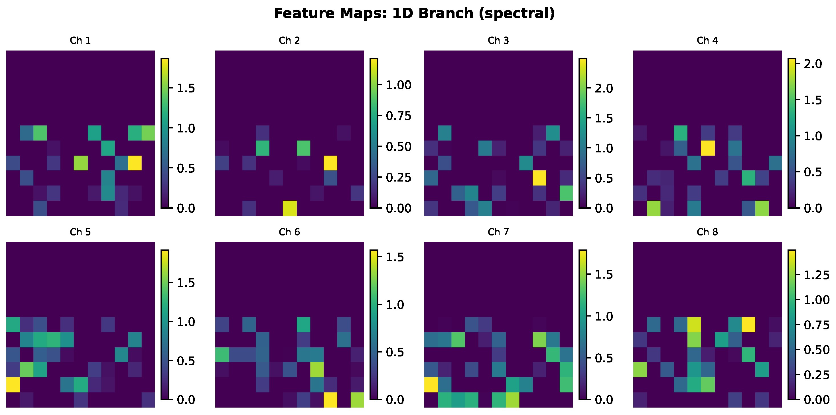
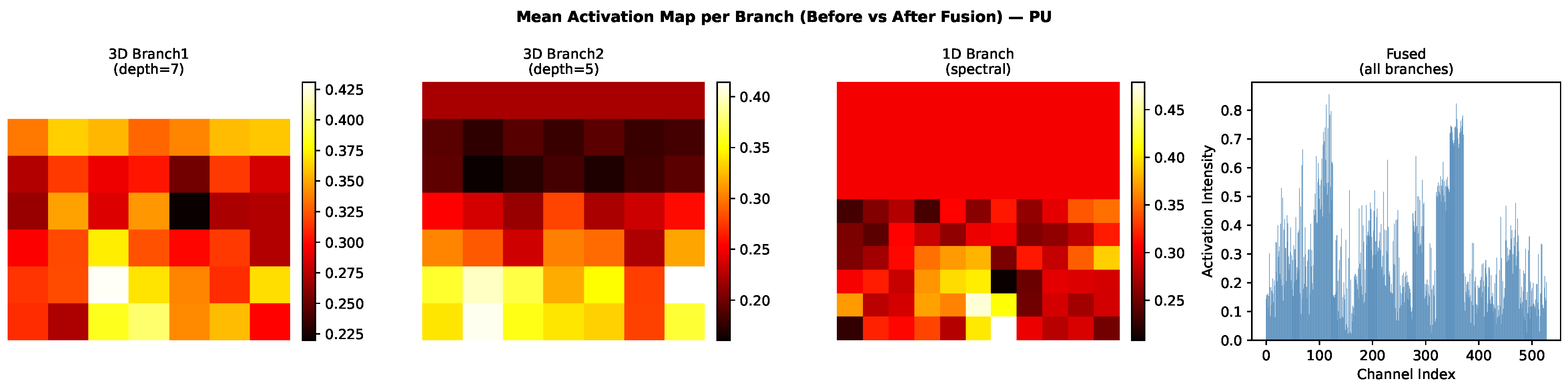
To further illustrate the behavior of MFEF, Figure 17, Figure 18, Figure 19 and Figure 20 visualize representative feature maps and activation distributions on the PU dataset. The three branches exhibit different response patterns, suggesting that they capture complementary information at different scales. After fusion, the resulting representation preserves discriminative responses while suppressing part of the noise, which is consistent with the quantitative results in Table 7. To further validate the stability of RDLNet beyond the fixed 30-samples-per-class protocol, we analyze performance under varying training sample sizes and examine whether the advantage of the MFEF module remains consistent across different sample regimes.

To further illustrate the internal mechanism of MFEF and verify that it effectively avoids over-smoothing, Figure 17, Figure 18 and Figure 19 visualize representative feature maps from the individual 3D and 1D branches on the PU dataset. The visualizations reveal distinct and complementary response patterns: the 3D convolutional branches effectively capture multi-scale spatial–spectral context, while the 1D branch preserves fine-grained spectral discriminability independent of local spatial perturbations. Furthermore, as shown in Figure 20, after fusing these multi-dimensional features, the network successfully retains highly discriminative target activations while strongly suppressing background noise. This confirms that the proposed parallel multi-branch design extracts rich local details without suffering from the over-smoothing degradation typically seen in excessively redundant spatial architectures.

Table 8. Comparison of the mean values of rdlnet with and without ROP on five datasets (%).

Dataset	Strategy	OA	AA	Kappa
	Without ROP	83.59	88.60	78.96
PU	With ROP	82.29	89.22	77.32
	Difference	−1.30	+0.62	−1.64
	Without ROP	95.02	97.41	94.44
SA	With ROP	92.80	96.53	91.97
	Difference	−2.22	−0.88	−2.47
	Without ROP	93.16	96.28	91.51
Xuzhou	With ROP	91.54	95.00	89.42
	Difference	−1.62	−1.28	−2.09
	Without ROP	73.18	71.75	65.40
Honghu	With ROP	70.52	68.59	62.15
	Difference	−2.66	−3.17	−3.25
	Without ROP	92.45	94.21	90.54
Longkou	With ROP	90.82	92.54	88.28
	Difference	−1.63	−1.67	−2.26

further compares RDLNet with and without the ROP strategy on all five datasets. After applying ROP, the OA reduction remains moderate, ranging from 1.30% to 2.66% across datasets. This trend is much smaller than the performance drops observed for most comparative methods in Table 5 and Table 6. These results suggest that RDLNet is relatively stable under the proposed leakage-controlled setting and is better suited to ROP-reconstructed patches.

4. Discussion

The experimental results demonstrate that most comparative methods experience substantial performance degradation after applying the ROP strategy, whereas RDLNet remains consistently strong across all five datasets. This suggests that the proposed model is less dependent on overlap-induced leakage and is better able to learn discriminative representations from leakage-controlled patches. A possible reason lies in the design of the MFEF module. After ROP is applied, the reconstructed patches still preserve class-related spectral signatures, but their natural local spatial continuity is partially weakened. Under this condition, feature extractors that rely too heavily on intact local spatial patterns may become less effective. However, as highlighted by recent central attention mechanisms [27], the central pixel provides the primary and most decisive spectral information, while neighboring pixels serve mainly as auxiliary context. Because our ROP strategy strictly preserves the target central pixel while only modifying the overlapping surroundings, architectures with robust spectral–spatial fusion capabilities—like our proposed MFEF module combining 3D and 1D branches—can still effectively classify the target. In contrast, the proposed MFEF module combines two 3D branches and one 1D branch, which allows the network to jointly model spectral–spatial context while preserving fine-grained spectral discrimination.

The ablation results in Table 7 support this interpretation: the 3D + 1D combination achieves the best performance, whereas adding the 2D branch leads to a decline, likely because it introduces redundant or less compatible spatial features after ROP modifies the local neighborhood structure. The visualization results in Figure 17, Figure 18, Figure 19 and Figure 20 provide further evidence that different branches of MFEF capture complementary response patterns. After fusion, the resulting representation preserves discriminative activations while suppressing part of the noise, which is consistent with the quantitative improvements observed. In addition, Table 8 shows that the performance reduction of RDLNet after applying ROP remains moderate across datasets, further indicating that the proposed architecture is relatively stable under the leakage-controlled setting.

The reported standard deviations also help interpret the robustness of the proposed leakage-controlled evaluation. Since the variability aggregates the effects of random train/test sampling, replacement-pixel sampling in ROP, and model training dynamics, the relatively constrained deviations of RDLNet indicate that the proposed MFEF design adapts well to the stochastic perturbations introduced by patch reconstruction. By contrast, the larger deviations observed for some comparative methods imply that their predictions are more sensitive to specific reconstructed neighborhood configurations, suggesting a stronger dependence on fragile local spatial patterns. Therefore, the standard deviation should be interpreted together with the mean result: methods with strong average performance and relatively small deviations are more convincing under the proposed leakage-controlled strategy.

Despite the effectiveness of the MFEF module in mitigating overlap-induced leakage, the proposed ROP strategy and the RDLNet architecture still present certain limitations. First, ROP replaces overlapping neighbors with the same-class training pixels from other spatial locations, which inevitably weakens the natural spatial continuity of the patch. Therefore, ROP is better viewed as a leakage-controlled patch reconstruction strategy rather than a perfect surrogate for natural scene structure. In practice, ROP is particularly suitable for small-sample settings where preserving training samples is more critical than preserving exact local spatial continuity. Second, ROP assumes that pixels from the same class are sufficiently similar to serve as replacements, which may be less suitable for classes with strong intra-class variability.

Furthermore, limitations also exist within the architectural configurations. In this work, all experiments are conducted under a fixed patch size of $11\times 11$, and PCA is used as a preprocessing step for dimensionality reduction. As shown in Table 4, the optimal PCA dimension still needs to be selected manually for different datasets. Additionally, to further examine the trade-off between recognition performance and model complexity,

Table 9. Model complexity comparison on PU dataset (pca = 30, patch size = 11 × 11).

Model	Parameters	FLOPs
1D-CNN	55.1 K	57.1 K
2D-CNN	76.9 K	1.06 M
3D-CNN	6.12 M	16.12 M
RDLNet	5.24 M	10.06 M

reports a representative comparison with 1D-CNN, 2D-CNN, and 3D-CNN on the PU dataset under the setting of PCA = 30 and patch size $11\times 11$. As expected, RDLNet is more complex than simple 1D and 2D CNN baselines, but it requires fewer parameters and fewer FLOPs than the 3D-CNN baseline while achieving substantially better recognition performance under the ROP-based setting. These results indicate that RDLNet does not pursue minimal complexity, but achieves a favorable accuracy–efficiency trade-off among representative CNN-based models.

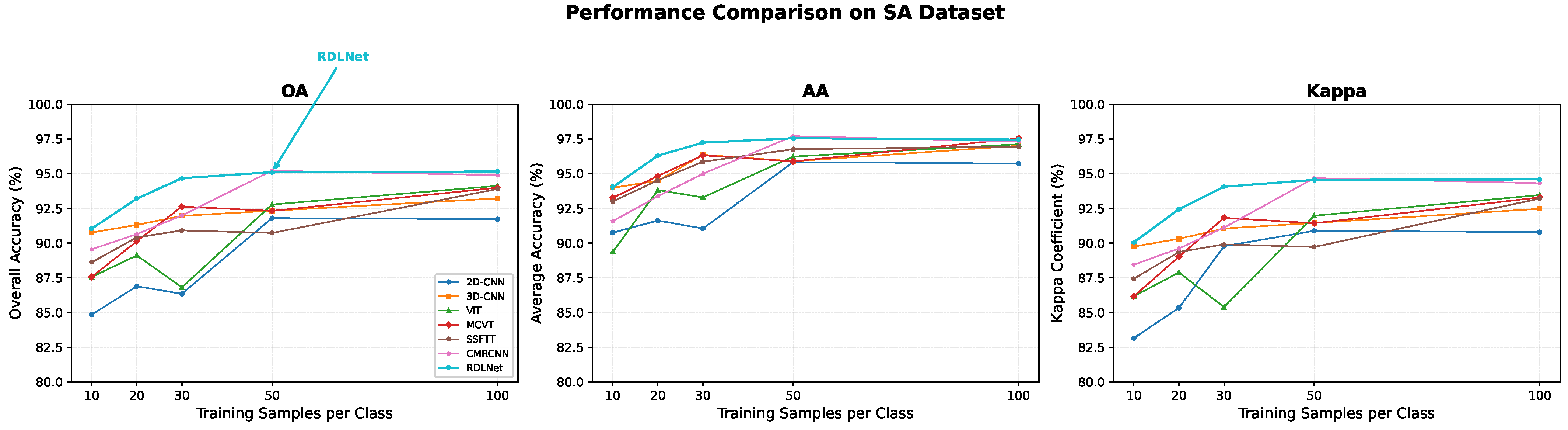
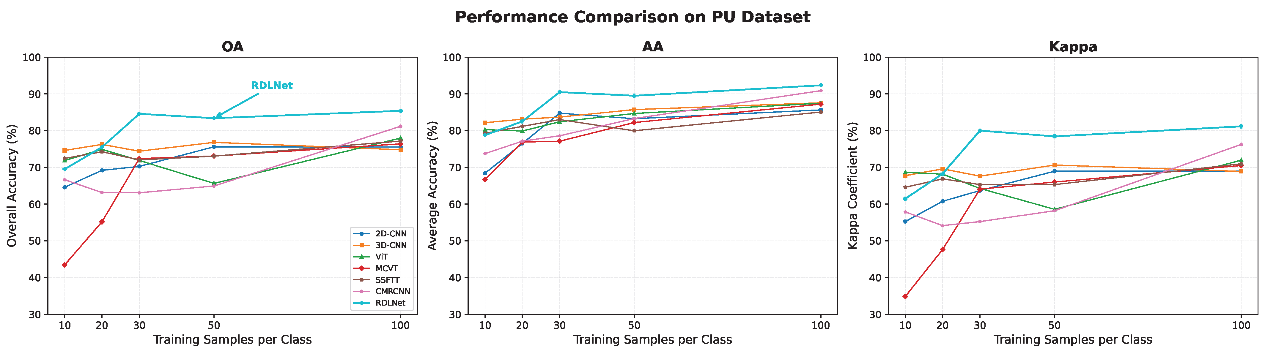
To further validate the stability of RDLNet and ensure its advantages are not restricted to the fixed few-shot protocol (i.e., 30 samples per class), we evaluated the model’s performance under varying training sample sizes, ranging from 10 to 100 samples per class. As illustrated by the performance curves in Figure 21 and Figure 22 for the SA and PU datasets, respectively, RDLNet consistently maintains a clear competitive margin over the baseline methods across all tested sample regimes. This stable upward trajectory indicates that the multi-dimensional convolution design of the MFEF module is universally effective for feature extraction on leakage-controlled patches, rather than being a hyperparameter artifact optimized solely for extremely low-sample constraints.

Looking ahead, future work may proceed in several directions. A more systematic comparison between ROP and spatially disjoint sampling would help clarify their relative advantages in terms of sample efficiency and spatial realism. It would also be highly beneficial to explore adaptive dimensionality selection instead of manually choosing PCA dimensions for each dataset. Finally, extending the proposed framework to accommodate variable patch sizes, broader remote sensing tasks, or more lightweight backbone architectures will further enhance its practical applicability.

5. Conclusions

This paper revisits the train–test overlap problem in patch-based hyperspectral image classification, demonstrating that conventional random patch splitting can lead to overly optimistic performance evaluations due to data leakage. To address this critical issue, we propose the replacing overlapping pixels (ROP) strategy, which reconstructs patch data in a leakage-controlled manner while preserving the standard patch-based input format. Furthermore, to effectively model these reconstructed patches, we designed the Resolving Data Leakage Network (RDLNet), featuring a Multiple Feature Extraction and Fusion (MFEF) module that seamlessly integrates multi-scale 3D and 1D convolutions.

Extensive experiments across five public hyperspectral datasets reveal a stark reality: while existing state-of-the-art methods suffer significant performance degradation once overlap-induced leakage is eliminated, RDLNet maintains consistently high and robust accuracy. The multi-branch design successfully captures complementary spectral–spatial features without over-smoothing, and its superiority persists across varying training sample sizes, proving its stability beyond extreme few-shot conditions.

Ultimately, this study not only provides a highly effective classification architecture but also highlights the pressing need for fair, leakage-free benchmarking protocols in the HSI community. Future research will build upon this foundation by exploring adaptive dimensionality reduction techniques and extending the proposed leakage-controlled framework to broader remote sensing tasks and variable spatial scales.