


Highlights
What are the main findings?
- This paper systematically reviews machine learning algorithms for snow cover recognition, detailing the process of extracting semantic features and marking the first comprehensive survey from a machine learning perspective.
- It categorizes algorithms based on task objectives, comparing their strengths and weaknesses across optical remote sensing, SAR, passive microwave, and multi-source data fusion tasks, while also providing an in-depth analysis of attention mechanisms and transformer architectures for future advancements.
What are the implications of the main findings?
- As a review from a machine learning standpoint, it establishes a foundational framework for researchers, consolidating current methodologies and highlighting key techniques for snow cover analysis.
- By offering a task-oriented comparison and emphasizing emerging architectures like transformers, it guides the optimization of multi-source data fusion and points toward innovative directions for leveraging deep learning in snow monitoring applications.
Abstract
Snow plays a significant role in the global energy balance, climate change, hydrological cycles, and other areas. However, traditional surface observation methods are limited in capturing the spatiotemporal dynamics of snow. This paper systematically reviews Machine Learning algorithms applicable to snow cover recognition. It highlights traditional Machine Learning methods such as Support Vector Machines and Random Forests, as well as more semantically oriented Deep Learning methods, including CNNs, attention mechanisms, and Transformers. These methods have shown robust performance in the domain of snow identification. Lastly, the paper discusses the strengths and weaknesses of different approaches and suggests directions for future research. Through this paper, readers will gain a comprehensive understanding of Machine Learning-based snow recognition algorithms and how these algorithms can be leveraged better.
1. Introduction
Snow is a key natural resource that influences the Earth’s climate and water cycle [1]. During winter, about 40–50% of the Northern Hemisphere is covered by snow [2], affecting the global radiation balance, groundwater, glaciers, and human activities [3]. Snow’s high reflectivity and low thermal conductivity strongly affect the energy exchange between the surface and atmosphere [4]. At the same time, snow cover also directly affects ecological and socio-economic systems, controlling runoff mechanisms and affecting plant and animal ecosystems [5].
Given the significant impact of snow on Earth’s climate and water cycle, accurate monitoring and understanding of snow coverage is crucial. This paper focuses on snow recognition using satellite data, specifically addressing two tasks: Fractional Snow Cover (FSC) and Binary Snow Cover (BSC). FSC quantifies the ratio of snow-covered area within each pixel, while BSC determines the presence or absence of snow in each pixel.
The continuous development of satellite technology has provided more access for acquiring high-precision snow cover information across various regional and temporal scales [6]. Remote sensing methods for observing snow cover can be categorized into optical remote sensing, passive microwave remote sensing, and active microwave remote sensing, based on the type of sensor used. Given the strengths and limitations of each approach, it is essential to provide a detailed comparison to guide their optimal use.
Researchers have conducted extensive research on optical remote sensing [2]. A key development in this area is the Normalized Difference Snow Index (NDSI) [7], as described below, which leverages the distinct spectral characteristics of snow—high reflectance in visible light and low reflectance in the short-wave infrared spectrum:
where b4 and b6 are the 4th and 6th bands of MODIS. In this algorithm, snow cover indicates when NDSI > 0.4. From 1995 to 2007, references [8,9,10,11] found that applying this empirical algorithm to different global surfaces makes it challenging to eliminate uncertainties arising from complex variations in surface cover types. Moreover, due to the spectral similarities in the shortwave infrared band, distinguishing between clouds and snow becomes challenging as empirical algorithms depend solely on spectral data.
Compared to optical data, microwave remote sensing technology exhibits greater stability under the influence of cloud cover, weather changes, and lighting conditions [12]. Microwave remote sensing can be divided into active microwave and passive microwave. Traditionally, the main passive microwave radiative models used for snow detection include Chang’s method [13], the multi-layer snow microwave emission transmission model [14], and the HUT snow emission model [15]. In active microwave remote sensing, Synthetic Aperture Radar (SAR) stands out as a prominent technology [16]. Traditional methods primarily identify snow based on the differences in backscatter coefficients between snow and other terrains across various polarizations and frequencies. Another approach involves using interferometric measurement techniques to detect snow by analyzing the differences in coherence coefficients before and after snowfall [17].
Both optical and microwave data share a common issue: there is no universal function to represent the complex nonlinear relationship between remote sensing data and snow cover [18,19]. A more general and robust scientific framework is required to solve the problem.
In recent years, the rapidly developing theory of Machine Learning (ML) has provided a solid methodology for snow detection technologies [20]. ML is characterized by its strong nonlinear fitting ability, enabling fast computation speeds and high generalization capabilities. It can effectively integrate the advantages of empirical algorithms and spectral analysis algorithms, offering considerable potential for optimization [21].
Currently, remote sensing data are becoming more diverse, heterogeneous, and complex, challenging traditional Machine Learning methods to adequately model the nonlinear relationships between inputs and outputs [22]. As a result, Deep Learning (DL) methods are emerging as an important area of research in remote sensing [23]. DL excels in extracting semantic information, making it particularly suitable for handling large-scale satellite data [24,25,26,27].
Prior to this paper, there have been several excellent review articles focusing on snow cover recognition. The study [28] firstly gave a brief overview of the physical properties of snow and, secondly, described commonly used methods for snow recognition, which were empirical algorithms and linear regression algorithms based on spectral data. The article primarily focused on optical data. The study [29] categorized snow identification algorithms based on SAR technology into three main groups: (1) wet snow detection based on SAR backward scattering characteristics; (2) PolSAR technology that inverts the scattering mechanism of the target snow pattern; (3) the coherence value computed by InSAR technology, which allows the estimation of the total SCE. It introduced aspects of traditional ML algorithms and primarily focused on SAR.
Based on the existing reviews, this paper updates and supplements the recent advances in snow recognition algorithms, focusing on the Machine Learning algorithms, classified into traditional ML and DL algorithms [30]. Snow detection tasks, based on data type, can be categorized into tasks based on optical remote sensing, SAR remote sensing, passive microwave remote sensing, and tasks based on multi-source data. This paper will analyze the specific tasks and summarize the development process of these algorithms. Additionally, the paper also summarizes common datasets used for snow remote sensing, outlines related work for the four tasks, and analyzes the evaluation metrics in snow detection tasks.
This paper focuses on snow cover extent and helps readers understand the development of snow recognition algorithms based on Machine Learning, comparing the advantages and disadvantages of various algorithms. At the same time, it summarizes potential algorithms of computer vision that can be applied to snow detection. This paper makes the following contributions:
(1) It introduces popular Machine Learning algorithms and focuses on the specific process of extracting features. To our knowledge, this is the first review article that systematically introduces snow recognition algorithms from a Machine Learning perspective.
(2) The paper categorizes from the perspective of task objects and introduces algorithms for optical tasks, SAR tasks, passive microwave tasks, and multi-source data fusion tasks separately.
(3) The paper details the developmental relationships between different snow detection algorithms and points out future directions for development.
As shown in Figure 1, the remainder of this paper is organized as follows. Section 2 presents related work on snow detection, including the primary tasks, commonly used snow datasets and ML methods, accuracy evaluation metrics, and a Citespace survey. Section 3 and Section 4 introduce snow detection algorithms based on traditional Machine Learning and Deep Learning methods, respectively, unfolding according to the four task directions. Section 5 summarizes the issues with existing algorithms and proposes future research directions.
Figure 1.
Overall structure of this paper.
2. Related Work
2.1. Four Tasks in Snow Recognition
Extracting valuable information from remote sensing data has become a highly focused research topic—remote sensing interpretation is an important part of it, involving classifying and identifying targets in the images, such as residential areas, vegetation, ground cover, water bodies, bridges, ships, and aircraft. Achieving automation and intelligence in remote sensing interpretation has long been a goal pursued by researchers.
In remote sensing tasks, since these ML models often exhibit limited generalization and transferability across multimodal data, there is a need to modify or design different models according to the specific data sources or target types [31]. Therefore, this paper categorizes tasks from the perspective of the data used.
2.1.1. Optical Tasks
The task of snow recognition in optical images started earlier, mainly due to the following advantage:
(1) Visually natural and easy to interpret. Optical images provide high-resolution surface information showing targets’ location, size, shape, texture, and other characteristics [32]. It makes optical images visual and easy to interpret and understand.
However, the optical snow recognition task also suffers from the following challenges:
(1) Optical sensors are affected by weather and lighting conditions [33]. Cloud can lead to missing and blurred areas in optical images, and dark conditions at night wil reduce image quality.
(2) Confusion between snow, ice, and clouds. In optical images, snow, ice, and clouds appear to have similar spectral and textural features, resulting in classification algorithms being unable to identify them accurately [34].
2.1.2. SAR Tasks
SAR has the following advantages in snow accumulation recognition tasks:
(1) Unlike optical remote sensing, SAR can penetrate clouds and measure the surface in all weather and lighting conditions. These capabilities are valuable regarding snow monitoring, as snow covered areas are often cloudy and subject to polar darkness in winter.
(2) Compared to optical remote sensing, SAR can extract polarization and phase information, providing unique insights into the Earth’s surface, including surface textures, moisture content, and geometric structures.
However, there are some drawbacks:
(1) SAR systems are based on the principle of coherence, which results in speckle noise, and this speckle noise is inevitable [35].
2.1.3. Passive Microwave Tasks
Passive microwave remote sensing has the following advantages in snow detection tasks:
(1) Passive microwave remote sensing has high temporal resolution, which allows for frequent and consistent monitoring of snow-covered areas [36].
(2) Passive microwave sensors can penetrate clouds, fog, and most weather conditions, providing reliable data [12].
However, passive microwave also has its drawbacks:
Due to the longer wavelengths, the spatial resolution of passive microwave is usually not as high as optical remote sensing [37]. This means that passive microwave has certain limitations in capturing fine surface features.
2.1.4. Multi-Source Tasks
The core of the collaborative application of multi-source data is the fusion analysis [38]. It is necessary to explore the fusion method to use the rich information. Based on the stage at which data fusion analysis occurs, it can be divided into three levels: pixel level, feature level, and decision level [39].
(1) Pixel-level fusion. In pixel-level fusion, the aim is to fuse data from different sources to the same pixel to obtain more information. This fusion level requires solving problems such as geometric distortion, radiometric correction, and image alignment between different source images.
(2) Feature-level fusion. Feature-level fusion combines feature information from different sources to enhance an image’s feature representation and information content.
(3) Decision-level fusion. Decision-level fusion combines classification results from different sources based on separate classifiers or decisions to produce a more integrated and reliable decision.
Researchers primarily concentrate on feature and decision fusion in the fusion analyses of SAR and optical remote sensing. These techniques are predominantly employed for large-scale regional classification [40]. When deploying multisource data in pixel-level tasks, one faces registration issues, consistency problems, and noise issues.
Table 1 summarises the advantages and disadvantages of the four tasks [41].
Table 1.
Comparison of the advantages and disadvantages of four tasks.
2.2. Datasets
This section collects available snow cover datasets that can be used for Machine Learning, as shown in Table 2.
Table 2.
Summary of datasets.
2.2.1. Optical Datasets
(1) MOD10A1/MOD10A2: The MODIS products are currently the most widely used, encompassing various types of global snow cover monitoring products [42]. They offer products with a spatial resolution of 500 m. MOD10A1 provides daily snow cover data, while MOD10A2 offers an 8-day composite of the MOD10A1 snow cover product [43].
(2) Snow_cci: It includes time series data of Snow Cover Fraction from MODIS and AVHRR sensors. The daily SCF products derived from MODIS data offer a spatial resolution of 0.01 degrees (approximately 1 km) for the period between 2000 and 2020, while those from AVHRR data provide a resolution of 0.05 degrees (about 5 km) covering the years 1982 to 2018.
(3) CSWV Dataset: The CSWV Dataset is the first free high-resolution remote sensing image semantic segmentation dataset used for cloud and snow detection, based on Worldview-2 satellite images. The data can be obtained from source [44]. The resolution of this dataset primarily ranges from 0.5 to 10 m and includes 27 high-resolution remote sensing cloud and snow images. The shooting locations are mainly in the Cordillera Mountains of North America, with the time distribution from June 2014 to July 2016. The image background is complex and diverse, including forests, grasslands, lake areas, and bare land. The types of snow mainly include permanent snow, stable snow, and intermittent snow.
(4) Landsat8 SPARCS (L8 SPARCS): This dataset was created by M. Joseph Hughes from Oregon State University, as indicated by source [45]. Collected by the Landsat-8 satellite, the dataset primarily consists of remote sensing image data of 1000 × 1000 size for 80 different scenes. These are categorized into five classes: clouds, cloud shadows, water bodies, background, and snow/ice.
(5) Cloud-free MODIS Snow Cover Dataset (MODIS SC): This dataset was developed by completely removing clouds through a series of spatiotemporal filters and the Variational Interpolation algorithm from the MODIS satellite’s snow cover product (MOD10C1), as mentioned in source [46]. The dataset has a temporal resolution of one day and a spatial resolution of 0.05°. The capture locations are above the continental United States, mainly including Seattle, Minneapolis, the Rocky Mountains, and the Sierra Nevada. The time distribution spans from March 2000 to February 2017.
(6) HRC_WHU: The dataset was created by the SENDIMAGE laboratory at Wuhan University [47]. It contains 150 high-resolution remote sensing images of large scenes. Each image contains RGB channels, distributed in various regions of the world, including vegetation, snow, desert, urban, and water. The image resolution is mainly between 0.5 and 15 m.
(7) GlobSnow: The European Space Agency (ESA) funded GlobSnow-1 project was active from 2008 to 2012. The currently on-going GlobSnow-2 project is a direct continuation of the GlobSnow-1 and will continue through May 2014. The current Snow Extent dataset is based on optical data from Envisat AATSR and ERS-2 ATSR-2 sensors covering the Northern Hemisphere between 1995 to 2012.
2.2.2. SAR Datasets
(1) LSD4WSD: This dataset is an open dataset for wet snow detection [48]. The data come from Sentinel-1 satellite SAR images acquired over the French Alps from August 2020 to August 2021 and consist of 487,157 training samples of size 16 × 16 and 3668 test samples, for each of which the labels are obtained from the Crocus physical model. Each sample has nine channels, including three polarization channels (VV, VH, VV, and VH combined), three terrain features (elevation, orientation, and slope), and polarization ratios for each of the three polarization channels.
(2) SWS Dataset: SWS is generated from C-band SAR data from the Sentinel-1 satellite, which provides a wet-snow range over the European alpine region with a spatial resolution of 60 m. It is not possible to distinguish between dry and flaky snow from C-band SAR data alone, so they are combined into one category.
2.2.3. Passive Microwave Datasets
(1) SSM/I: The Special Sensor Microwave/Imager is a widely used passive microwave radiometer system onboard the Defense Meteorological Satellite Program satellites. It provides Brightness Temperature data at multiple frequencies. Passive microwave data are particularly valuable for snow monitoring as it can penetrate clouds and operate independently of solar illumination, making it highly effective for estimating snow depth and Snow Water Equivalent.
(2) AMSR-E/AMSR2: The Advanced Microwave Scanning Radiometer for EOS on the Aqua satellite and its successor AMSR2 on the GCOM-W1 satellite provide global passive microwave measurements. They offer improved spatial resolution and broader spectral coverage compared to SSM/I, contributing significantly to global snow cover mapping and climate research.
2.3. Machine Learning
2.3.1. Support Vector Machine
Support Vector Machines are a binary classification model based on interval-maximizing linear classifiers in feature space [49]. The learning strategy of SVM is to maximize the intervals by solving a convex quadratic programming problem and equivalently minimizing a regularized loss function, which involves solving a convex quadratic programming optimization problem. In the remote sensing snow recognition task, the simple objective is to classify the pixel points in the remote sensing image into two categories, snow and non-snow, which are highly compatible with the SVM algorithm.
The SVM algorithm inputs the training data of snow and snow-free pixels. It separates different classes of samples by tracking maximally spaced hyperplanes in the kernel space of the sample mapping. To achieve the best robust performance, the algorithm maximizes the spacing between hyperplanes by minimizing the value of W [50] in Figure 2.
Figure 2.
Schematic representation of the feature Hilbert space after model selection.
Denote the training samples by , where , denotes an N-dimensional space, n is the number of available samples, and i is the ith available sample. In the binary classification task, the , −1 denotes the semantic category of snow accumulation, and +1 denotes the semantic category of non-snow. Given a nonlinear mapping , it seeks to solve the following:
Restricted:
The parameters and b define the linear classifiers in the feature space, and denotes the positive slack variables with allowable error ranges. The nonlinear mapping is appropriately chosen to ensure the linear separability of the transformed samples in the feature space. The parameter c determines the generalization ability of the classifier.
2.3.2. Random Forest
The Random Forest classifier is an ensemble classifier that utilizes a collection of CARTs (Classification and Regression Trees) for prediction [51] as in Figure 3. These trees are generated by sampling a subset of training data points with replacement (a bagging approach). It means the same data sample might be selected multiple times, while others may not be selected at all. Most of the samples, termed in-bag samples, are utilized for training the trees. The remaining samples, referred to as out-of-bag samples, are employed in an internal cross-validation procedure to estimate the performance of the resulting RF model [51].
Figure 3.
The workflow of Random Forest.
Each decision tree is independently grown without any pruning, and each node is split using a randomly selected subset of features(Mtry). By constructing the forest with a user-defined number of trees (Ntree), the algorithm produces trees with high variance and low bias [52]. The final classification decision is made by averaging the class probabilities calculated by all the trees generated. Consequently, when evaluating a new unlabeled data point, it is assessed against all decision trees in the ensemble, with each tree contributing to a vote for a class. The class with the maximum votes is ultimately selected.
At the time of writing, the Random algorithm has been implemented in many software packages [53], which will be summarized in Table 3:
Table 3.
Random Forest software package.
2.3.3. Convolutional Neural Network
A Convolutional Neural Network is a classical Deep Learning model initially designed for image processing and computer vision endeavors as in Figure 4. It comprises convolutional, pooling, and fully connected layers, collectively offering robust capabilities for feature extraction and representation [71]. Using convolutional operations, CNN systematically extracts local features from images, while pooling operations facilitate the gradual aggregation of higher-level semantic insights [72]. In the context of snow recognition, CNNs autonomously acquire snow-associated features encompassing attributes like texture, shape, and boundaries.
Figure 4.
The workflow of a Convolutional Neural Network.
LeNet [73] and AlexNet [74] represent seminal CNN architectures that established the foundational framework of CNNs and played a pivotal role in advancing Deep Learning. The subsequent emergence of network architectures like VGG [75], ResNet [76], and others have further enriched model depth and elevated performance. Moreover, an array of innovative network architectures and techniques continues to evolve, including the Inception series [77], Xception [78], MobileNet [79], and EfficientNet [80], all oriented toward optimizing the model depth, parameter count, and overall efficiency [81].
2.4. Evaluation Metrics
Model accuracy assessment evaluates the performance of a trained model and is an important part of the model development process [82].
Binary snow recognition divides each pixel into snow-covered or snow-free. To evaluate the accuracy of binary snow identification, confusion matrices are commonly used [83]. The definition of the confusion matrix is presented in Table 4:
Table 4.
Definition of confusion matrix in accuracy evaluation.
In general, four categories are often used:
(1) True Positive, Pixel predicted and labeled values are snow, noted as A.
(2) False Positive, labeled with a value of no snow, but predicted to be snowy, noted as B.
(3) False Negative, where no snow is predicted but snow is actually present, is recorded as C.
(4) True Negative, where both predicted and labeled values are free of snow, denoted as D.
Considering that remote sensing data sometimes experience partial data missing, parameters E and F have been added.
Based on the basic statistical results of the confusion matrix, secondary metrics have been derived to evaluate the strengths and weaknesses of the model. The definitions of these secondary metrics are as outlined in Table 5.
Table 5.
Level-2 index of confusion matrix.
Precision refers to the proportion of pixels correctly identified as snow among all pixels predicted as snow. Recall refers to the proportion of pixels that were correctly predicted as snow out of all actual snow pixels. Accuracy is the most commonly used performance metric, representing the proportion of correctly classified pixels out of all pixels. However, when the number of categories is unbalanced, the larger categories often become the main factor affecting Accuracy. To address this limitation, the Kappa coefficient is utilized. It measures the consistency between the predicted results and the true labels while accounting for the agreement occurring by chance, making it particularly robust for evaluating models on imbalanced datasets. MIoU is a common evaluation metric in the field of semantic segmentation, used to assess the similarity between the predicted results and the true labels. The F-score metric considers both precision and recall.
In FSC (Fractional Snow Cover) tasks, the RMSE (Root Mean Squared Error), MBE (Mean Bias Error), and MAE (Mean Absolute Error) are also commonly used, as shown in Table 6, where n is the number of samples, represents the actual values, and represents the predicted values for each sample. RMSE quantifies the average magnitude of prediction errors and is particularly sensitive to large errors. MBE indicates the average bias in predictions, identifying systematic overestimations or underestimations. MAE measures the average absolute errors, offering a clear depiction of typical error magnitude without being unduly influenced by large individual errors.
Table 6.
Common metrics used in FSC tasks.
In the following section, these evaluation metrics will be used.
3. Traditional Machine Learning-Based Methods
In this section, we provide an overview of the workflow involved in traditional Machine Learning approaches in Figure 5. We will discuss the typical steps, from data preprocessing and feature engineering to model training and evaluation. Understanding this workflow is essential for gaining insights into how traditional Machine Learning methods are applied in various tasks.
Figure 5.
Workflow of traditional Machine Learning approaches.
Compared to Deep Learning, traditional Machine Learning methods are more complex in feature engineering, and the feature selection stage is more challenging [84]. Traditional Machine Learning has the following three advantages:
(1) Low sample requirements: Traditional Machine Learning algorithms have a simple model structure, a small number of variables, and robust data utilization capabilities to use limited data to learn features and patterns thoroughly. With limited data, traditional Machine Learning algorithms often outperform Deep Learning methods.
(2) Low computational resources: Unlike Deep Learning that relies on high-performance GPUs, traditional Machine Learning requires low computational resources.
(3) Strong interpretability: Traditional Machine Learning involve direct manual design and selection of features in feature engineering, which makes these algorithms easier to explain and understand [85].
This section will introduce research on traditional Machine Learning in snow recognition.
3.1. Optical Task
3.1.1. Feature Extraction Methods for Optical Tasks
In traditional Machine Learning, feature engineering is a crucial step, which usually requires manual selection and extraction of features. This process not only demands extensive expertise but is also vital for the successful implementation of algorithms.
Wu et al. [86] noted that the edges of cloud pixels are typically smooth and soft. However, the shape of snow is often very sharp, influenced by the terrain in mountainous areas. To utilize this significant difference, they proposed a feature called the Curvature Histogram (CH), which describes the edge degree of each pixel. The feature implementation process can be divided as follows:
(1) A template is applied to every edge pixel to measure its curvature. The background pixels within this template are excluded from the calculations. The template used for curvature evaluation can be represented as:
(2) The curvature degree for each edge pixel is evaluated using the following equation:
where N denotes the value obtained by applying the template to the edge pixel, and the constant corresponds to the scenario where the edge undergoes the smoothest change.
(3) Upon identifying all edge pixels, the CH of the boundary points set is calculated. This CH quantifies the proportions of edge points with varying degrees of curvature within the set, serving as an indicator of whether the object’s boundary shape is smooth or sharp.
Furthermore, the authors also combined spectral, texture, and shape features, summarized in Table 7.
Table 7.
Features extracted in [86].
Wang et al. [90] directly utilize the individual spectral bands of Sentinel-2 satellite data as independent optical features, avoiding the cumbersome manual feature extraction and focusing on finding the optimal band feature combination. In most cases, clouds and snow cannot be distinguished through RGB three channels alone. Therefore, the authors, by comparing the reflectance distribution of snow, clouds, and background across the 12 spectral bands of the Sentinel-2 L2A product, select B2 (Blue), B11 (SWIR1), B4 (Red), and B9 as the four-band combination. In the case of cloud presence, the cloud mask which comes with each Sentinel-2 product can be used to remove cloud areas. Experimental results indicate that this four-band combination performs better in the RF model than both the RGB band combination and all 12 band combinations, while also avoiding the trend of overfitting.
Similarly, Xia et al. [91], like [90], directly use raw images as a recognizable data form for ML. Inspired by the convolutional networks, they adopt dilated convolutional windows of different granularities to scan the original data for feature extraction. This feature extraction method enlarges the receptive field without losing the original graphic’s texture and spatial correlation information. Compared to [90], it reduces the amount of computational parameters and speeds up the computation. The extracted features are divided through the Gini coefficient, selecting key feature classes. As illustrated in Figure 6, the overall features input into the left-side RF model, with selected features sent into the right-side RF model, obtaining the final results through an n-level cascading forest. Specifically, to effectively distinguish highly similar cloud and snow pixels, this method leverages multi-grained scanning across multi-spectral bands to simultaneously capture fine spatial textures and subtle spectral differences. Experimental results demonstrate that this approach significantly outperforms traditional machine learning and standard convolutional networks, achieving an optimal balance between high recognition accuracy and computational efficiency.
Figure 6.
Framework of RES-gcforest.
Mohd et al. [92] utilize Hyperion hyperspectral images for feature extraction. First, they employ the Minimum Noise Fraction (MNF) method to reduce data dimensions and remove noise. Then, they evaluate the purity of each pixel through the Pixel Purity Index (PPI), aiming to identify the most pure pixels in the image. Subsequently, they apply n-dimensional visualization techniques to map high-dimensional data to a lower-dimensional space, facilitating researchers in observing the data structure. Finally, endmembers are extracted through spectral unmixing algorithms, providing input data for Machine Learning algorithms. This series of processes improves the quality and availability of image information, laying the foundation for image classification and target recognition tasks.
Regardless of the traditional Machine Learning model used, these feature methods can be effectively applied, thus playing a role in a wide range of Machine Learning tasks. The cross-model applicability emphasizes the importance of feature extraction techniques in enhancing algorithm performance. Table 8 summarizes the research of the authors mentioned above.
Table 8.
Summary of feature extraction methods in optical tasks.
3.1.2. Application and Optimization in Optical Scenes
The application and optimization of Machine Learning algorithms across diverse optical scenes remains a critical focus in remote sensing. In mountainous areas, factors such as tree shadows and forest cover severely impact the accuracy of snow detection algorithms. Researchers have increasingly utilized targeted Machine Learning methods to address these environmental challenges.
Zhu et al. [93] employed a stepwise optimization scheme: initially, they trained a primary SVM model (SVM1) to differentiate sunlit snow from other objects. Subsequently, a secondary SVM model (SVM2) was utilized specifically to identify snow obscured by shadows. This stepwise strategy significantly improves overall accuracy in rugged terrains because sunlit snow and shadowed snow exhibit drastically different spectral signatures (shadowed snow often has lower reflectance and a bluish tint due to Rayleigh scattering). By decoupling this bimodal distribution into two separate classification spaces, the model effectively avoids the underfitting that occurs in single global classifiers, although its limitation is the potential for error propagation from the first step to the second.
Barella et al. [94] focused on mountainous regions affected by heavy shadows, sun glint effects, and atmospheric disturbances. They simplified the data collection process based on an improved Normalized Difference Snow Index (NDSI) proposed in their study, selecting representative samples tailored to specific acquisition conditions. The main analytical advantage of this guided sampling is that it forces the model to learn from challenging boundary cases (like glint and shadow) rather than being biased by large numbers of “easy” pure snow pixels, thereby enhancing the model’s robustness and accuracy in complex atmospheric conditions.
In multi-temporal scenarios, studies such as [95,96] shift the focus toward utilizing time-series satellite imagery to capture the dynamic changes in snow-covered areas over time. Reference [95] introduced a method based on Collaborative Expectation Maximization and Support Vector Machine (Co-EM-SVM). As illustrated in Figure 7, this approach first treats two images as distinct descriptions of the same surface and divides them into two complementary subsets. Then, a small set of labeled samples is used from these subsets to train independent classifiers. Subsequently, each classifier makes predictions on unlabeled samples and uses these predictions to mutually enhance training. Through iterative updates until accuracy requirements are met or the maximum number of iterations is reached, this design allows both classifiers to learn from the unlabeled data, thereby significantly improving performance. The core advantage of this temporal co-training is its ability to overcome the severe scarcity of multi-temporal labels. By dynamically adapting the decision boundary using unlabeled data, the model generalizes much better to shifting snowlines across different dates, though its limitation is that mutual learning may collapse if both temporal views are heavily obscured by clouds.
Figure 7.
Diagram of co-training architecture for multi-temporal extensions.
Unlike the decision-level fusion strategy in [95], reference [96] employed a feature-level fusion approach, as shown in Figure 8. This workflow involves extracting sample locations from multiple images taken at the same time point to create an initial training dataset. It then performs joint feature selection to identify the most relevant input features, optimizes the training dataset to enhance the model’s learning efficiency, and finally executes joint parameter optimization to ensure the classifier parameters are optimally configured. This process results in several independent classifiers, each tailored for a specific task, to maximize the accuracy of snow detection. Compared to single-date models, this multi-temporal ensemble feature fusion directly improves accuracy by mitigating the impact of transient noise, such as moving clouds or temporary sensor errors. By leveraging temporal continuity, it prevents the classifier from overfitting to a specific seasonal snow state, yielding a more stable global accuracy.
Figure 8.
Multi-temporal ensemble learning framework.
The aforementioned strategies effectively address the challenges posed by complex environmental factors, thereby improving both the accuracy and efficiency of snow recognition. Furthermore, in optical tasks, studies [91,95] demonstrated that Random Forest (RF) generally outperforms SVM and ANN, particularly in forested and mountainous applications. This is largely because RF, as an ensemble of decision trees, is inherently more robust to outliers and noisy data (like scattered forest gaps) than the hyperplane-based SVM. Nonetheless, compared to the traditional NDSI method, all three Machine Learning schemes exhibit vastly superior performance.
Moreover, reference [97] explored the performance of different SVM kernel functions in snow detection tasks. The commonly used kernels in SVM are categorized into four types: linear, polynomial, radial basis function (RBF), and sigmoid. The authors concluded that, in remote sensing tasks, the RBF and polynomial kernels typically yield better results. The analytical reason for this superiority lies in their capacity to handle highly nonlinear spectral decision boundaries. While linear kernels underfit the complex spectral confusion between snow, clouds, and highly reflective bare rocks, the RBF kernel maps features into an infinite-dimensional space, effectively isolating clustered and irregular snow pixel distributions. Table 9 presents the optimal training settings and comparative performance of these various kernel functions.
Table 9.
Optimal training settings for SVM kernel functions.
Table 10 summarizes the application and optimization of Machine Learning algorithms in the task of optical snow detection.
Table 10.
Application and optimization of Machine Learning algorithms in optical snow detection tasks.
3.2. SAR Tasks
Traditional Machine Learning algorithms have been applied to SAR data processing, particularly in the classification and snow line monitoring of glacier and snow-covered regions [98,99,100,101,102].
Reference [103] has proven that, compared to X and L band polarization features, C-band data possess higher capability, efficiency, and reliability in surface object recognition tasks. This is fundamentally because the C-band strikes an optimal balance in penetration depth: it is highly sensitive to the liquid water content in wet snow while avoiding the excessive ground penetration of the L-band and the superficial atmospheric scattering of the X-band. References [98,99] utilized C-band quad-polarization data from the RADARSAT-2 satellite and adopted similar SAR data preprocessing methods. The preprocessing session in [99] is divided into three steps:
(1) Absolute calibration of polarized SAR images is performed using the look-up table provided in the product;
(2) The image is filtered using a fine Lee sigma filter to suppress scattering noise;
(3) Orthorectification of images using SAR simulated terrain correction method and DEM data involves the following four processes:
[a] Simulation of SAR images from DEM based on the imaging geometry of real SAR images;
[b] Automatic matching of reliable tie points appearing in real and simulated SAR images;
[c] Distortion of the real SAR image into a simulated image using a polynomial function fitted from the connection points;
[d] Using the DEM to project the distorted real SAR image back to the map coordinate system.
The outcome of the entire process is an orthorectified SAR image within the DEM map coordinate system. When dealing with SAR images obtained from non-flat terrain, it is imperative to incorporate terrain information into the radiometric correction process. The standardized method for removing the effect of the local incidence angle is to use a backscatter model and an incidence angle map derived from the DEM and satellite orbit information instead of the estimated incidence angle used in the raw data processing. Here is the formula provided:
where is the angle of incidence measured from the elliptic curve, is the actual angle of incidence calculated from the DEM, and is the backscattering coefficient of the original SAR image. This radiometric terrain correction is analytically indispensable for mountainous snow detection. Because SAR is a side-looking active sensor, steep terrain inherently causes severe radiometric distortions. By normalizing the backscattering coefficient, the model prevents topography-induced brightness variations from being misclassified as physical changes in snow cover.
After preprocessing data, due to the difficulty in distinguishing between ice and snow using traditional backscatter characteristics, references [98,99] employed a target decomposition strategy, applying both Pauli decomposition and H/A/ decomposition to the backscatter features to extract new characteristics. The core advantage of these decompositions is their ability to shift the feature space from simple signal intensity to physical scattering mechanisms (such as surface, double-bounce, and volume scattering). This allows classifiers to distinguish snow from bare ice or rock based on how the radar wave interacts with the target’s internal structure, significantly elevating the classification ceiling compared to using raw backscatter alone.
Callegari et al. [100] proposed a more comprehensive processing scheme for fully polarized SAR data for extracting from it the features needed for the SVM classifier, as shown in Figure 9. The scheme is divided into three steps:
Figure 9.
The preprocessing scheme of quad-polarization SAR data.
(1) By using the radar brightness lookup table provided in the product, the Sinclair matrix S for each pixel is obtained. In order to extract physical information from the Sinclair matrix S, it can be represented as a target vector based on a set of complex basis matrices. The polarimetric Pauli coherence matrix and the polarimetric Lexicographic covariance matrix are generated through the outer product of the target vector and its conjugate transpose.
(2) Speckle noise is filtered through multi-view processing and Lee filter.
(3) Feature information is extracted through Touzi decomposition and Cloude–Pottier decomposition. The Cloude–Pottier decomposition is a common polarimetric decomposition method used for feature extraction and target recognition in polarimetric synthetic aperture radar images. The Touzi decomposition is a roll-invariant, incoherent decomposition method proposed to address the ambiguity of specific scattering mechanisms in Cloude–Pottier decomposition. Terrain correction is performed using DEM data, and all features are fused and input into the SVM classifier. By fusing these advanced polarimetric features, the SVM classifier gains a highly multidimensional physical description of the snowpack, maximizing accuracy. However, the critical limitation of quad-polarization schemes is the inherently narrow swath width of the satellite and the massive computational cost required for covariance matrix generation.
Compared to quad-polarization data, Sentinel-1 C-band dual-polarization data have lower data costs and computational burdens. However, due to the limited polarization information, dual-polarization SAR still has significant uncertainties in distinguishing between dry snow and wet snow [100]. This limitation arises because dual-pol configurations often lack the complete cross-polarization phase information required to fully characterize complex volume scattering.
Reference [104] uses features such as the backscattering ratio, InSAR coherence, and PolSAR H/A/ parameters, along with topographical parameters (elevation, aspect, slope, and curvature), and land cover information to initially identify snowy parts. Afterwards, Nagler’s method [105] is utilized to differentiate between dry and wet snow. The integration of InSAR coherence is a major analytical breakthrough here: since dry snow is virtually transparent to C-band microwaves but wet snow strongly absorbs them, the sudden drop in interferometric coherence provides a highly reliable temporal indicator for wet snow transition.
Compared to [104], reference [102] opts for a data-driven approach. It introduces an MRF model to optimize SVM classification results, ensuring spatial consistency within local areas and reducing random errors and noise impacts during classification. Since snow cover naturally forms continuous surfaces rather than fragmented speckles, the MRF acts as a spatial regularizer. It penalizes isolated misclassified pixels caused by inherent SAR speckle noise, structurally preventing the “salt-and-pepper” artifacts that typically degrade pixel-wise SVM classifications, effectively improving the accuracy of distinguishing between wet snow and dry snow.
Aside from the C-band data, reference [101] demonstrates the potential of Ku-band SAR data from the SCATSAT-1 satellite in snow detection tasks, achieving promising results with the SVM classifier as well. Due to its shorter wavelength, the Ku-band is significantly more sensitive to the volume scattering of dry, shallow snow than the C-band, offering a highly advantageous complementary data source for global dry snow mapping despite its susceptibility to atmospheric attenuation.
Table 11 summarizes the application of traditional Machine Learning in SAR tasks.
Table 11.
Summary of traditional Machine Learning applications in SAR tasks.
3.3. Passive Microwave Tasks
Microwave radiation covers the spectral range from 0.1 to 100 cm (300 to 0.3 GHz ) [106]. According to Rayleigh’s principle, energy with longer wavelengths exhibits very small scattering intensity. Compared to microwave wavelengths, clouds, fog, aerosols, and other gas molecules have relatively smaller particle sizes, thus causing minimal interference with emitted microwave radiation [107]. These advantages make microwave sensors an optimal choice for monitoring the Earth’s surface objects’ emitted signals, regardless of weather conditions. Passive microwave (PMW) sensors are able to detect microwave radiation from snow cover, which can be converted into brightness temperature signals, then further analyzed to retrieve various information [108].
Previous studies have used brightness temperature (TB) data to determine binary snow cover information. Liu et al. [109] briefly introduced seven commonly used algorithms for binary snow cover identification using TB data, which differ in determined threshold values and classification categories. Grody et al. [110] were the first to combine passive microwave and Machine Learning methods to identify snow pixels, analyzing microwave brightness temperature data against known surface features to establish classification standards and create decision trees to eliminate non-snow pixels. According to this method, by selecting appropriate brightness temperature thresholds and excluding non-scattering bodies, as well as surfaces affected by rainfall, cold deserts, and permafrost, the extracted area can then be identified as snow-covered.
Subsequently, reference [110] inverted binary snow cover maps using BP neural networks. Reference [110] collected brightness temperature data from SSM/I as input, selecting the China Meteorological Station Observation (CMSO) dataset and the Global Surface Summary of Day (GSOD) product as ground observation data. A total of 75% were chosen as training samples, with the remaining used as test samples. The training samples were input into the BP neural network for training, and the trained ANN model was used to predict the probability of each pixel being covered by snow in the test samples.
However, only a few studies have been directly dedicated to inverting the FSC map from TB data. In earlier research [111], RF was used to estimate FSC from EASE-Grid brightness temperature data. The research involved 19, 37, 91 GHz horizontal and vertical polarization as well as 22 GHz vertical polarization. The experiments validated that using TB data to estimate the proportion of snow-covered area at subpixel level is feasible. However, reference [111] lacked further analysis of the response process of TB inversion to FSC changes. On this issue, reference [112] first explored the relationship between FSC and TB through a radiative transfer model. The study found that no universal function could adequately describe the nonlinear and complex relationship between FSC-TB across six channels (19, 37, and 91 GHz vertical and horizontal polarization). Then, an FSC retrieval algorithm using the extreme random trees method and RF was designed to utilize TB data and DEM auxiliary information to improve predictions of subpixel snow-covered areas. Through a series of comparison and evaluation experiments, the established FSC retrieval model showed promising capabilities in FSC estimation, with the highest correlation coefficient (R = 0.728) and the lowest mean absolute error (MAE = 0.158) and root mean square error (RMSE = 0.204). At the same time, the derived binary snow cover product from FSC performed quite well in classifying snow cover in North America (overall accuracy = 0.884).
Table 12 summarizes the application of traditional Machine Learning in passive microwave tasks.
Table 12.
Summary of traditional Machine Learning applications in passive microwave tasks.
3.4. Multi-Source Tasks
Optical remote sensing of snow cover fully utilizes the unique spectral characteristics of snow, but differentiating snow from clouds remains a challenge. Unlike optical methods, microwave remote sensing is less affected by cloud cover, weather, and light conditions due to its high penetration capability. Although microwave remote sensing has this advantage, current passive microwave sensors have a relatively coarse spatial resolution compared to optical sensors. SAR, however, provides higher spatial resolution than passive microwave sensors. Many researchers have conducted more accurate snow monitoring through the heterogeneous data fusion of optical and SAR data.
IHe et al. [17] proposed an SVM for extracting snow in rugged mountains based on SAR and optical data The authors first processed the SAR and optical data with ENVI and SARScape, corrected the SAR images based on coherence, local incidence angle, etc., and then geographically aligned the SAR and optical data to obtain matched snow and snow-free samples without clouds and shadows.
The authors extracted SAR data features based on interferometric coherence analysis and proposed the definition of coherence C as follows:
indicates the difference in radar platforms, which can be measured by the difference in the Doppler frequency of the radar beams.
indicates the azimuth angle, which can be obtained by calculating the Doppler frequency difference.
indicates the thermal noise of the sensor system, including gain and antenna characteristics.
indicates baseline.
indicates the data processing algorithm.
indicates sensor geometry effects caused by orbit differences between InSAR data pairs.
indicates the temporal correlation caused by changes in the ground surface and depends on the standard deviation in the direction of distance and height.
He et al. pointed out that HH and VV polarizations exhibit greater coherence differences between snow and snow-free pixels than HV and VH polarizations and that VV polarization exhibits the same coherence properties as HH polarization; the authors chose the HH-polarized coherent image to extract the snow. The coherence features of the extracted SAR image were inputted into the SVM for training with the subpadding features of the optical image to achieve snow accumulation recognition. The whole process is shown in Figure 10. The experimental results showed that the algorithm was greatly affected by the subsurface of the measured area, and the average accuracy of snow extraction using this method was 83.8% and 77.5% in areas with low and high vegetation cover, respectively.
Figure 10.
Flowchart of the SVM method based on SAR and optical data.
In 2017, Hu et al. [113] built on previous work by focusing their research on distinguishing dry snow and wet snow. The study proposed a two-step approach based on quad-polarized SAR and optical remote sensing data for identifying dry and wet snow cover in mountainous areas. Firstly, based on the dry snow and snow-free areas observed by the GF-1 satellite as the reference standard, the relationship between polarization patterns, local incidence angles, and the types of underlying surfaces and coherence was determined. A dynamic thresholding algorithm was then used to extract snow cover. Secondly, 36 polarization parameters were extracted using various polarization decomposition methods, and it was found that some of these parameters exhibited high separability between dry and wet snow. Based on these parameters and field-measured sample data, an SVM classifier was established to classify the snow cover.
However, this method heavily relies on prior knowledge obtained from field measurements and optical data, which is a common issue faced by supervised classification methods.
The authors of [114] also focused on snow recognition in mountainous areas, introducing the PROBA-V satellite’s vegetation indices LAI and FVC with MODIS and Sentinel-1 data, verifying its value in snow detection tasks.
Compared to the above methods, which relied on manually selecting and combining features, [115] employed the Principal Component Analysis (PCA) technique to automatically filter out the most representative snow feature combination from SAR and optical data and used it as the input for SVM. This approach effectively simplified the feature selection process, enhancing the efficiency and accuracy of the model.
Table 13 summarizes the application of traditional Machine Learning in multi-source tasks.
Table 13.
Summary of traditional Machine Learning applications in multi-source tasks.
4. Deep-Learning-Based Methods
In recent years, Deep Learning methods have been widely applied in the field of image recognition due to their powerful classification performance, feature learning capabilities, and end-to-end structural design [116,117]. Experts and scholars have treated snow as a specific type of remote sensing semantic. Consequently, semantic segmentation algorithms for remote sensing imagery, which leverage Deep Learning methodologies, have experienced rapid development [118].
The workflow of Deep Learning approaches is demonstrated in Figure 11.
Figure 11.
Workflow of Deep Learning approaches.
4.1. Optical Tasks
Cloud and snow segmentation is highly critical yet challenging in optical remote sensing [119]. The primary difficulty lies in the “same spectrum, different objects” phenomenon: both cloud and snow exhibit extremely high reflectance in visible bands and share highly similar visual colors and local texture patterns. Consequently, traditional threshold-based methods relying purely on low-level spectral features often fail to accurately differentiate snow from cloud at the pixel level. To address this issue, recent studies [25,120,121] have demonstrated that Deep Learning techniques exhibit significant advantages. Specifically, they differentiate the two by leveraging high-level semantic context—recognizing that snow strictly conforms to underlying terrain and topography, whereas clouds suspend above the surface with distinct edge morphological characteristics and shadow distributions.
In 2017, Zhan et al. [120] first segmented snow and clouds using a framework based on Convolutional Neural Networks (CNN). The authors utilized the VGG network [75] as the feature extraction framework, replacing VGG’s initial fully connected layers with upsample layers to adapt semantic segmentation tasks. They highlighted that using fully connected layers causes problems, such as high computational cost and loss of positional information, since fully connected layers contain a large number of parameters when processing numerous pixels, and integrating information into a vector results in loss of spatial location information.
They believed that low-level features carry rich spatial information, helping to more precisely capture target boundaries and details, whereas high-level features contain richer semantic information, conducive to distinguishing different object categories. Based on this, they developed a strategy by upsampling and merging multi-scale feature information, as shown in Figure 12. By merging multi-scale features, the network effectively compensates for the morphological variability of clouds. It utilizes high-level semantics to identify large-scale cloud distributions while relying on low-level spatial details to accurately delineate the jagged boundaries of mountain snow, thereby mitigating the misclassification caused by their similar spectral reflectance.
Figure 12.
Modified VGG network.
They conducted experiments using a dataset constructed from Gaofen-1 satellite data. The results showed that, compared to SVM and MLP, the proposed model achieved significant improvements on the mIOU metric, reaching 90.6%, which validated the feasibility of Deep Learning technology in cloud and snow detection tasks.
As the layers of Deep Learning networks deepen, gradient vanishing and model degradation become common issues [76]. Addressing this challenge, ResNet [76] provided a solution by introducing a residual structure. Furthermore, Xia et al. [121] optimized the residual structure as shown in Figure 13, and their study showed that the optimized residual structure outperforms the original design in terms of classification performance and convergence speed. Especially in cloud and snow recognition tasks, the M-ResNet model proposed by [121] demonstrated superior accuracy compared to SVM and Random Forest (RF) models. The introduction of the residual structure ensures that the delicate textural differences between snow and clouds are not lost during deep forward propagation. This allows the network to maintain high sensitivity to the underlying surface textures of snow-covered areas, effectively preventing the common issue where thick clouds are mistakenly identified as snow patches due to feature degradation. In contrast, the SVM model had severe misidentification issues in non-snow areas, although the RF model improved this, but the misjudgment phenomenon was still significant.
Figure 13.
Comparison of the original residual and pre-activated residual unit.
According to advanced technologies from computer vision, reference [25] used ResNet as the core backbone network and integrated the Atrous Spatial Pyramid Pooling (ASPP) module [122] to cloud and snow detection tasks. The ASPP module (shown in Figure 14), typically located at the end of the Convolutional Neural Network, handles feature maps. Its novelty lies in capturing rich global and local contextual information at multiple spatial sampling rates through different scales of pooling operations. Since clouds in optical imagery exhibit extreme variations in scale and thickness, the multi-scale pooling operations of the ASPP module can simultaneously capture the macroscopic spatial distribution of a massive cloud system and the local contextual texture of fragmented snow patches, significantly reducing the spectral confusion at varying scales.
Figure 14.
Atrous Spatial Pyramid Pooling Unit.
Similar to how [102] used the MRF model to optimize SVM classification results in Chapter 3, reference [27] employed the CRF model to enhance the classification effectiveness of the Deeplab V3+ model [122]. The CRF model is particularly suited for capturing local connectivity within images. Compared to MRF, CRF supports more complex feature representations and more flexible conditional dependency modeling. It can handle not only the spatial relationships between pixels but also incorporate additional feature information such as color, texture, and edges. This conditional dependency modeling is exceptionally crucial for addressing the boundary blurring problem between semi-transparent clouds, cloud shadows, and actual snow cover. By enforcing spatial and color consistency, the CRF module effectively refines the jagged and fragmented segmentation edges typically produced by standard CNNs in mixed cloud–snow regions.
This paper also utilized some of the current mainstream CNN architectures and conducted work on the HRC_WHU dataset. Figure 15 below displays the segmentation effects of some mainstream models. The purple part is the cloud and cloud shadow, and the white part is the snow. (a) Input optical image, (b) label, (c) Resnet-50, (d) Deeplab V3+, (e) ExtremeC3, (f) UNet, (g) LinkNet.
Figure 15.
Comparison on the HRC_WHU with some CNN architectures. (a) Input optical image, (b) label, (c) Resnet-50, (d) Deeplab V3+, (e) ExtremeC3, (f) UNet, (g) LinkNet.
Building on the idea of modeling local relevance in images presented in [102], integrating attention mechanisms [123] into CNN backbone networks has become a natural step towards further enhancing model performance. Attention mechanisms, inspired by studies on human vision, allow models to selectively focus on key areas within images, thereby allocating limited information processing resources to the most crucial elements of the image more efficiently [124].
Researchers in [125,126] introduced the Convolutional Block Attention Module (CBAM) [127] into cloud and snow recognition tasks. The results from [125,126] indicated that compared to using only the backbone networks, models integrated with CBAM achieved significant improvements in the MIoU metric by 0.13% and 0.84%, respectively.
Specifically, CBAM consists of two key parts, as shown in Figure 16: the channel attention model and the spatial attention model.
Figure 16.
The architecture of CBAM. The multiplication sign represents the element-by-element multiplication of vectors, the plus sign represents the element-by-element addition operation, and S represents the Sigmoid operation.
In the channel attention model, effective spatial information of clouds and snow is first aggregated using average pooling and max pooling operations. Then, this information is fed into a Multi-Layer Perceptron (MLP) network, which generates a channel attention vector corresponding to the channels that need to be enhanced or suppressed. By adaptively recalculating the channel weights, the model can actively suppress the specific spectral channel responses dominated by highly reflective thick clouds, while amplifying the distinct spectral signatures associated with snow and underlying terrain.
The spatial attention model focuses on location information and complements the channel attention [128]. In the spatial attention model, feature maps of single channels obtained from average pooling and max pooling operations are first concatenated. Then, through a convolutional layer, an effective spatial attention map is generated, indicating locations that need to be emphasized or suppressed. This spatially targeted attention acts as a dynamic mask, filtering out the pervasive “same spectrum, different objects” interference from cloud-obscured regions and forcing the network to concentrate its representational power on the actual topographic features of snow.
SENet [129], as an efficient channel attention mechanism, has been successfully applied in cloud and snow detection networks [130]. As a channel attention module, SENet generates a one-dimensional feature equal in number to the channels through a global max-pooling operation. These features are channel weights to adjust the feature channels of the original input. This channel-wise recalibration enables the network to automatically emphasize the subtle spectral bands where the reflectance of snow and clouds diverge, thus providing a more discriminative feature space for segmentation.
Furthermore, due to its scalability, the attention mechanism can be plug-and-play in different model architectures. Table 14 summarize some excellent attention mechanisms for readers.
Table 14.
Summarization of attention mechanism.
With the development of the Attention mechanism, Transformer [123], the first model based entirely on an attention mechanism, was proposed, which not only made a breakthrough in natural language processing, but also inspired computer vision.
The Transformer architecture consists of a multi-layer structure comprising stacked Transformer blocks, as shown in Figure 17. These blocks are fundamental units in the Transformer model and exhibit the following structural characteristics:
Figure 17.
The architecture of classical Transformer.
(1) Multi-head Self-Attention Mechanism: This mechanism empowers the Transformer to capture correlation information across various positions within the input sequence. It achieves this by linearly transforming the input sequence, calculating attention weights for each position concerning the others, and then combining the attention-weighted result with the original input. Multi-head self-attention allows the Transformer to learn distinct representations in multiple subspaces, thus effectively capturing relationships between inputs.
(2) Position-wise Feed-Forward Network: Integral to the Transformer Block, the FFN consists of two fully connected layers that introduce nonlinear transformations to enhance the model’s representation. Applied uniformly to each position in the input sequence, the feed-forward network better models the dependencies between positions.
(3) Layer Normalization Module: The Transformer Block applies layer normalization to the output of each sublayer. This process ensures training stability by normalizing each sample in terms of feature dimensions and helps mitigate issues like vanishing or exploding gradients.
(4) Residual Connectors: Residual connectors are implemented within each Transformer Block sublayer (self-attention and feed-forward networks). These connectors add the sublayer outputs to the inputs, preserving information from the original inputs. This design aids in efficient gradient propagation, preventing information loss and alleviating the challenge of gradient vanishing during training.
Collaborating these components in the Transformer Block facilitates the adaptive modeling of input sequences, allowing the model to capture long-range dependencies within sequences. This adaptive capability enhances representation and generalization, contributing to the effectiveness of the Transformer architecture.
Based on Transformer, Hu et al. [148] proposed a dual-branch network as in Figure 18, MCANet, which combines CNNs and EdgeViTs [149] to extract local and global features from images for the task of cloud and snow segmentation. The authors argue that CNNs are excellent at extracting local information but lack accuracy in capturing global context. The characteristics of Transformers can address this shortcoming. Relying solely on local convolutional operations often leads to misclassifying isolated cloud clusters as snow patches due to their visual similarity. The self-attention mechanism of the Transformer resolves this by modeling long-range dependencies, granting the network the global receptive field necessary to comprehend whether a highly reflective region is part of a continuous airborne cloud system or a topographic mountain snowpack. Moreover, to facilitate training and reduce the model size, the authors employed lightweight EdgeViTs, which implement a downsampling operation before the Multi-head attention.
Figure 18.
The architecture of MCANet. Retrieved from Hu et al. (2023) [148] with permission.
The following Table 15 summarizes the applications of Deep Learning in optical tasks.
Table 15.
Applications of Deep Learning in optical tasks.
4.2. SAR Tasks
Despite the extensive application of SAR in object-level recognition tasks such as ship detection and large-scale agricultural coverage [150,151,152,153], its suitability is limited for pixel-level snow recognition. Noise issues are more prominent in SAR images, increasing the difficulty of distinguishing between snow and background. Additionally, labeling SAR images is both complex and time-consuming, making it challenging to ensure accuracy in annotations. Research on this topic is relatively scarce.
4.3. Passive Microwave Tasks
The integration of Deep Learning techniques with passive microwave data has been widely applied in fields such as snow depth and snow water equivalent estimation [154,155]. However, this study aims to explore the use of these technologies to identify snow coverage areas, laying the groundwork for more in-depth analysis of snow depth and other parameters. Regrettably, research literature on identifying snow coverage areas remains relatively scarce.
4.4. Multi-Source Tasks
A number of emerging technologies show great potential for detecting the extent of snow cover.
Lidar has shown great potential in the field of snow remote sensing. The unique Lidar system is not limited by sunshine conditions and cloud cover and provides accurate 3D data of snow [156]. Compared to other technologies, Lidar has the ability to penetrate parts of vegetation, allowing accurate measurement of the snow cover under forest. This is particularly critical for snow monitoring in mountain areas [157].
GNSS technology is also applied in snow remote sensing. Reference [158] shows that the change in snow depth can be clearly tracked through a GPS signal. The global coverage of GNSS technology allows it to monitor snow cover changes over a large area, which has important implications for water management and climate change research on a global scale. In addition, the flexibility and scalability of GNSS equipment allows it to be easily integrated with other remote sensing technologies, enhancing its application potential in snow monitoring and analysis [159].
To date, Deep Learning has not made significant progress in snow identification with multi-source data, which is mainly limited by the lack of heterogeneous datasets specifically for snow cover. However, in other domains of remote sensing, many Deep Learning frameworks for data fusion have achieved excellent results. In future, if datasets are established, some mature multi-modal Deep Learning frameworks may provide effective methods and have implications for snow identification tasks.
The following Table 16 summarizes open source Deep Learning algorithms based on multi-source data:
Table 16.
Application of Deep Learning to multi-source tasks in remote sensing.
5. Summary and Outlook
Machine Learning, as a data-based learning paradigm [167], plays a crucial role in remote sensing snow recognition tasks. The ongoing efforts of scholars from all over the world have led to significant advances in snow identification technology.
From the perspective of research methods, traditional Machine Learning focuses on optimal feature extraction and identification by simulating the nonlinear relationship between feature and snow cover. However, the end-to-end model based on Deep Learning technology can automatically extract features directly from remote sensing images to accurately identify snow coverage.
Among the four tasks, optical remote sensing is the most studied, which is especially closely combined with computer vision-based Deep Learning technology, and has been widely used in semantic segmentation tasks. However, its sensitivity to cloud interference cannot be ignored, which makes cloud snow segmentation a focus issue. Compared with optical remote sensing, SAR remote sensing is not subject to cloud interference, and associated research mainly focuses on extracting backscattering coefficient and different polarization characteristics from SAR data. Compared with using the entire optical image as input, the demand for computing resources is lower, so a large number of studies can obtain a good accuracy rate based on traditional Machine Learning. However, due to the speckle noise of the SAR image, its application in snow semantic segmentation is still limited. Passive microwave remote sensing is widely used in retrieving snow depth and equivalent snow water. In multi-source tasks, most of the current research focuses on the combination of features extracted from different remote sensing sources, and there are relatively few studies on the direct input of multiple heterogeneous image data into neural networks for multi-mode fusion.
Future snow cover studies can be enhanced in several ways as follows:
(1) Establish a large-scale snow dataset suitable for Deep Learning: Given the high dependence of Deep Learning on the quality of datasets [168], the lack of a snow dataset based on heterogeneous data currently limits its application in multi-source tasks. There is an urgent need to collect more diverse snow data, covering different regions, seasons and environmental conditions, to support more comprehensive studies.
(2) Research on multi-modal data fusion: Multi-modal technology can overcome the limitations of a single modal approach and provide more comprehensive information. In view of the breakthrough of multi-modal Deep Learning in optical, radar, SAR and other fields, multi-modal technology should be further explored for application to snow identification.
(3) Leverage large foundation models and vision models: Furthermore, the rapid emergence of large foundation models, particularly vision models such as the Segment Anything Model (SAM) [169], presents a transformative opportunity for remote sensing. In the context of snow identification, these foundational models exhibit powerful zero-shot generalization capabilities, which could significantly reduce the reliance on extensive pixel-level annotated datasets. Adapting such large-scale vision models to multimodal satellite imagery holds immense potential for improving cross-sensor adaptability and achieving more robust snow cover mapping in complex terrains in the future.
Author Contributions
Conceptualization, K.H., Z.Z. and K.M.; methodology, K.M. and K.H.; formal analysis, K.M., Z.Z., N.W. and T.G.; investigation, K.M. and Z.Z.; writing—original draft preparation, K.M.; writing—review, K.H. and Z.Z.; writing—editing, T.G. and Q.L.; visualization, K.M., K.H. and Z.Z.; supervision, K.H. and Z.Z.; project administration, K.H. and N.W.; collection of material, T.G. and Q.L.; All authors have read and agreed to the published version of the manuscript.
Funding
The research was supported by the Project of China Geological Survey (Grant No. DD202601103504) and the Deep Earth Probe and Mineral Resources Exploration—National Science and Technology Major Project of China (2025ZD1011400).
Data Availability Statement
No new data were created or analyzed in this study. Data sharing is not applicable to this article.
Acknowledgments
The financial support of Nanjing Ta Liang Technology Co., Ltd. and Nanjing Fortune Technology Development Co., Ltd. is deeply appreciated. The authors would like to express heartfelt thanks to the reviewers and editors who submitted valuable revisions to this article.
Conflicts of Interest
The authors declare no conflicts of interest.
References
- You, Q.; Wu, T.; Shen, L.; Pepin, N.; Zhang, L.; Jiang, Z.; Wu, Z.; Kang, S.; AghaKouchak, A. Review of snow cover variation over the Tibetan Plateau and its influence on the broad climate system. Earth-Sci. Rev. 2020, 201, 103043. [Google Scholar] [CrossRef] [Scilit]
- Dumont, M.; Gascoin, S. Optical Remote Sensing of Snow Cover. In Land Surface Remote Sensing in Continental Hydrology; Elsevier: Amsterdam, The Netherlands, 2016; pp. 115–137. [Google Scholar] [CrossRef] [Scilit]
- Bokhorst, S.; Pedersen, S.H.; Brucker, L.; Anisimov, O.; Bjerke, J.W.; Brown, R.D.; Ehrich, D.; Essery, R.L.; Heilig, A.; Ingvander, S.; et al. Changing Arctic snow cover: A review of recent developments and assessment of future needs for observations, modelling, and impacts. Ambio 2016, 45, 516–537. [Google Scholar] [CrossRef] [Scilit] [PubMed]
- Thackeray, C.W.; Derksen, C.; Fletcher, C.G.; Hall, A. Snow and climate: Feedbacks, drivers, and indices of change. Curr. Clim. Chang. Rep. 2019, 5, 322–333. [Google Scholar] [CrossRef] [Scilit]
- Edwards, A.C.; Scalenghe, R.; Freppaz, M. Changes in the seasonal snow cover of alpine regions and its effect on soil processes: A review. Quat. Int. 2007, 162, 172–181. [Google Scholar] [CrossRef] [Scilit]
- Chen, B.; Xia, M.; Qian, M.; Huang, J. MANet: A multi-level aggregation network for semantic segmentation of high-resolution remote sensing images. Int. J. Remote Sens. 2022, 43, 5874–5894. [Google Scholar] [CrossRef] [Scilit]
- Hall, D.K.; Riggs, G.A.; Salomonson, V.V. Development of methods for mapping global snow cover using moderate resolution imaging spectroradiometer data. Remote Sens. Environ. 1995, 54, 127–140. [Google Scholar] [CrossRef] [Scilit]
- Hall, D.K.; Riggs, G.A.; Salomonson, V.V.; DiGirolamo, N.E.; Bayr, K.J. MODIS snow-cover products. Remote Sens. Environ. 2002, 83, 181–194. [Google Scholar] [CrossRef] [Scilit]
- Hall, D.K.; Riggs, G.A. Accuracy assessment of the MODIS snow products. Hydrol. Processes 2007, 21, 1534–1547. [Google Scholar] [CrossRef] [Scilit]
- Klein, A.G.; Barnett, A. Validation of daily MODIS snow cover maps of the Upper Rio Grande River Basin for the 2000–2001 snow year. Remote Sens. Environ. 2003, 86, 162–176. [Google Scholar] [CrossRef] [Scilit]
- Klein, A.G.; Hall, D.K.; Riggs, G.A. Improving snow cover mapping in forests through the use of a canopy reflectance model. Hydrol. Processes 1998, 12, 1723–1744. [Google Scholar] [CrossRef]
- Boukabara, S.A.; Weng, F.; Liu, Q. Passive microwave remote sensing of extreme weather events using NOAA-18 AMSUA and MHS. IEEE Trans. Geosci. Remote Sens. 2007, 45, 2228–2246. [Google Scholar] [CrossRef]
- Chang, T.; Gloersen, P.; Schmugge, T.; Wilheit, T.; Zwally, H. Microwave emission from snow and glacier ice. J. Glaciol. 1976, 16, 23–39. [Google Scholar] [CrossRef] [Scilit]
- Mätzler, C.; Wiesmann, A. Extension of the microwave emission model of layered snowpacks to coarse-grained snow. Remote Sens. Environ. 1999, 70, 317–325. [Google Scholar] [CrossRef] [Scilit]
- Pulliainen, J.T.; Grandell, J.; Hallikainen, M.T. HUT snow emission model and its applicability to snow water equivalent retrieval. IEEE Trans. Geosci. Remote Sens. 1999, 37, 1378–1390. [Google Scholar] [CrossRef] [Scilit]
- Snehmani; Singh, M.K.; Gupta, R.; Bhardwaj, A.; Joshi, P.K. Remote sensing of mountain snow using active microwave sensors: A review. Geocarto Int. 2015, 30, 1–27. [Google Scholar] [CrossRef] [Scilit]
- Guangjun, H.; Pengfeng, X.; Xuezhi, F.; Xueliang, Z.; Zuo, W.; Ni, C. Extracting Snow Cover in Mountain Areas Based on SAR and Optical Data. IEEE Geosci. Remote Sens. Lett. 2015, 12, 1136–1140. [Google Scholar] [CrossRef] [Scilit]
- Zhu, L.; Zhang, Y.; Wang, J.; Tian, W.; Liu, Q.; Ma, G.; Kan, X.; Chu, Y. Downscaling snow depth mapping by fusion of microwave and optical remote-sensing data based on deep learning. Remote Sens. 2021, 13, 584. [Google Scholar] [CrossRef] [Scilit]
- Xiao, X.; Zhang, T.; Zhong, X.; Shao, W.; Li, X. Support vector regression snow-depth retrieval algorithm using passive microwave remote sensing data. Remote Sens. Environ. 2018, 210, 48–64. [Google Scholar] [CrossRef] [Scilit]
- Largeron, C.; Dumont, M.; Morin, S.; Boone, A.; Lafaysse, M.; Metref, S.; Cosme, E.; Jonas, T.; Winstral, A.; Margulis, S.A. Toward Snow Cover Estimation in Mountainous Areas Using Modern Data Assimilation Methods: A Review. Front. Earth Sci. 2020, 8, 325. [Google Scholar] [CrossRef] [Scilit]
- Chen, J.; Xia, M.; Wang, D.; Lin, H. Double Branch Parallel Network for Segmentation of Buildings and Waters in Remote Sensing Images. Remote Sens. 2023, 15, 1536. [Google Scholar] [CrossRef] [Scilit]
- Chen, K.; Xia, M.; Lin, H.; Qian, M. Multi-scale Attention Feature Aggregation Network for Cloud and Cloud Shadow Segmentation. IEEE Trans. Geosci. Remote Sens. 2023, 61, 5612216. [Google Scholar]
- Zhu, X.X.; Tuia, D.; Mou, L.; Xia, G.S.; Zhang, L.; Xu, F.; Fraundorfer, F. Deep learning in remote sensing: A comprehensive review and list of resources. IEEE Geosci. Remote Sens. Mag. 2017, 5, 8–36. [Google Scholar] [CrossRef] [Scilit]
- Wieland, M.; Li, Y.; Martinis, S. Multi-sensor cloud and cloud shadow segmentation with a convolutional neural network. Remote Sens. Environ. 2019, 230, 111203. [Google Scholar] [CrossRef] [Scilit]
- Zheng, K.; Li, J.; Ding, L.; Yang, J.; Zhang, X.; Zhang, X. Cloud and Snow Segmentation in Satellite Images Using an Encoder–Decoder Deep Convolutional Neural Networks. ISPRS Int. J. Geo-Inf. 2021, 10, 462. [Google Scholar] [CrossRef] [Scilit]
- He, K.; Zhang, X.; Ren, S.; Sun, J. Spatial Pyramid Pooling in Deep Convolutional Networks for Visual Recognition. IEEE Trans. Pattern Anal. Mach. Intell. 2015, 37, 1904–1916. [Google Scholar] [CrossRef] [Scilit]
- Wang, Z.; Fan, B.; Tu, Z.; Li, H.; Chen, D. Cloud and Snow Identification Based on DeepLab V3+ and CRF Combined Model for GF-1 WFV Images. Remote Sens. 2022, 14, 4880. [Google Scholar] [CrossRef] [Scilit]
- Dietz, A.J.; Kuenzer, C.; Gessner, U.; Dech, S. Remote sensing of snow—A review of available methods. Int. J. Remote Sens. 2011, 33, 4094–4134. [Google Scholar] [CrossRef] [Scilit]
- Tsai, Y.L.S.; Dietz, A.; Oppelt, N.; Kuenzer, C. Remote Sensing of Snow Cover Using Spaceborne SAR: A Review. Remote Sens. 2019, 11, 1456. [Google Scholar] [CrossRef] [Scilit]
- Liu, P.; Choo, K.K.R.; Wang, L.; Huang, F. SVM or deep learning? A comparative study on remote sensing image classification. Soft Comput. 2016, 21, 7053–7065. [Google Scholar] [CrossRef] [Scilit]
- Brenning, A. Transforming feature space to interpret machine learning models. arXiv 2021, arXiv:2104.04295. [Google Scholar] [CrossRef] [Scilit]
- Dai, X.; Xia, M.; Weng, L.; Hu, K.; Lin, H.; Qian, M. Multi-Scale Location Attention Network for Building and Water Segmentation of Remote Sensing Image. IEEE Trans. Geosci. Remote Sens. 2023, 61, 5609519. [Google Scholar] [CrossRef] [Scilit]
- Hu, K.; Wang, T.; Shen, C.; Weng, C.; Zhou, F.; Xia, M.; Weng, L. Overview of Underwater 3D Reconstruction Technology Based on Optical Images. J. Mar. Sci. Eng. 2023, 11, 949. [Google Scholar] [CrossRef] [Scilit]
- Yue, J.; Fang, L.; Ghamisi, P.; Xie, W.; Li, J.; Chanussot, J.; Plaza, A. Optical Remote Sensing Image Understanding with Weak Supervision: Concepts, methods, and perspectives. IEEE Geosci. Remote Sens. Mag. 2022, 10, 250–269. [Google Scholar] [CrossRef] [Scilit]
- Xiao-Guang, Z.; Gang-Yao, K.; Jian-Wei, W. A Review of Polarimetric SAR Speckle Reduction. J. Image Graph. 2008, 13, 377–385. [Google Scholar]
- Joshi, N.; Baumann, M.; Ehammer, A.; Fensholt, R.; Grogan, K.; Hostert, P.; Jepsen, M.R.; Kuemmerle, T.; Meyfroidt, P.; Mitchard, E.T.; et al. A review of the application of optical and radar remote sensing data fusion to land use mapping and monitoring. Remote Sens. 2016, 8, 70. [Google Scholar] [CrossRef] [Scilit]
- Lusch, D.P. Introduction to Microwave Remote Sensing; Center for Remote Sensing and Geographic Information Science, Michigan State University: East Lansing, MI, USA, 1999. [Google Scholar]
- Ye, Y. Fast and robust registration of multimodal remote sensing images via dense orientated gradient feature. Int. Arch. Photogramm. Remote Sens. Spat. Inf. Sci. 2017, 42, 1009–1015. [Google Scholar] [CrossRef] [Scilit]
- Zhang, J. Multi-source remote sensing data fusion: Status and trends. Int. J. Image Data Fusion 2010, 1, 5–24. [Google Scholar] [CrossRef] [Scilit]
- Reiche, J.; Verbesselt, J.; Hoekman, D.; Herold, M. Fusing Landsat and SAR time series to detect deforestation in the tropics. Remote Sens. Environ. 2015, 156, 276–293. [Google Scholar] [CrossRef] [Scilit]
- Agrawal, S.; Khairnar, G. A comparative assessment of remote sensing imaging techniques: Optical, sar and lidar. Int. Arch. Photogramm. Remote Sens. Spat. Inf. Sci. 2019, 42, 1–6. [Google Scholar] [CrossRef] [Scilit]
- Liang, T.G.; Huang, X.D.; Wu, C.X.; Liu, X.Y.; Li, W.L.; Guo, Z.G.; Ren, J.Z. An application of MODIS data to snow cover monitoring in a pastoral area: A case study in Northern Xinjiang, China. Remote Sens. Environ. 2008, 112, 1514–1526. [Google Scholar] [CrossRef] [Scilit]
- Hall, D.K.; Riggs, G.A. MODIS/Terra Snow Cover Daily L3 Global 500 m SIN Grid, Version 6, 2016. Available online: https://nsidc.org/data/mod10a1/versions/6 (accessed on 30 March 2026).
- Zhang, G.; Gao, X.; Yang, Y.; Wang, M.; Ran, S. Controllably deep supervision and multi-scale feature fusion network for cloud and snow detection based on medium-and high-resolution imagery dataset. Remote Sens. 2021, 13, 4805. [Google Scholar] [CrossRef] [Scilit]
- Hughes, M.J.; Hayes, D.J. Automated detection of cloud and cloud shadow in single-date Landsat imagery using neural networks and spatial post-processing. Remote Sens. 2014, 6, 4907–4926. [Google Scholar] [CrossRef] [Scilit]
- Tran, H.; Nguyen, P.; Ombadi, M.; Hsu, K.l.; Sorooshian, S.; Qing, X. A cloud-free MODIS snow cover dataset for the contiguous United States from 2000 to 2017. Sci. Data 2019, 6, 180300. [Google Scholar] [CrossRef] [Scilit] [PubMed]
- Li, Z.; Shen, H.; Cheng, Q.; Liu, Y.; You, S.; He, Z. Deep learning based cloud detection for remote sensing images by the fusion of multi-scale convolutional features. arXiv 2018, arXiv:1810.05801. [Google Scholar]
- Hao, X.; Luo, S.; Che, T.; Wang, J.; Li, H.; Dai, L.; Huang, X.; Feng, Q. Accuracy assessment of four cloud-free snow cover products over the Qinghai-Tibetan Plateau. Int. J. Digit. Earth 2018, 12, 375–393. [Google Scholar] [CrossRef] [Scilit]
- Cortes, C.; Vapnik, V. Support-Vector Networks. Mach. Learn. 1995, 20, 273–297. [Google Scholar] [CrossRef] [Scilit]
- Gao, J.; Xu, L.; Huang, F. A spectral–textural kernel-based classification method of remotely sensed images. Neural Comput. Appl. 2015, 27, 431–446. [Google Scholar] [CrossRef] [Scilit]
- Breiman, L. Random forests. Mach. Learn. 2001, 45, 5–32. [Google Scholar] [CrossRef] [Scilit]
- Colditz, R.R. An Evaluation of Different Training Sample Allocation Schemes for Discrete and Continuous Land Cover Classification Using Decision Tree-Based Algorithms. Remote Sens. 2015, 7, 9655–9681. [Google Scholar] [CrossRef] [Scilit]
- Belgiu, M.; Drăguţ, L. Random forest in remote sensing: A review of applications and future directions. ISPRS J. Photogramm. Remote Sens. 2016, 114, 24–31. [Google Scholar] [CrossRef] [Scilit]
- Trimble. eCognition Developer 8.7.2. Reference Book, München; Trimble: Westminster, CO, USA, 2013. [Google Scholar]
- Trimble. Ecognition-Random Forest. 2013. Available online: https://www.sysdecoitalia.com/wp-content/uploads/2015/04/eCognition9.0.2_ReleaseNotes.pdf (accessed on 25 August 2025).
- R Development Core Team. R: A Language and Environment for Statistical Computing; R Foundation for Statistical Computing: Vienna, Austria, 2005; ISBN 3-900051-07-0. [Google Scholar]
- R-Development-Core-Team. R-Project Random Forest. 2005. Available online: http://www.r-project.org/ (accessed on 25 August 2025).
- Holmes, G.; Donkin, A.; Witten, I.H. Weka: A Machine Learning Workbench. In Proceedings of the Second Australian and New Zealand Conference on Intelligent Information Systems, Brisbane, Australia, 29 November–2 December 1994; pp. 357–361. [Google Scholar]
- Weka. 1994. Available online: https://weka.sourceforge.io/doc.dev/weka/classifiers/trees/RandomForest.html (accessed on 25 August 2025).
- Pedregosa, F.; Varoquaux, G.; Gramfort, A.; Michel, V.; Thirion, B.; Grisel, O.; Blondel, M.; Prettenhofer, P.; Weiss, R.; Dubourg, V. Scikit-Learn: Machine Learning in Python. J. Mach. Learn. Res. 2011, 12, 2825–2830. [Google Scholar]
- Scikit-Learn Random Forest. 2011. Available online: https://scikit-learn.org/stable/modules/generated/sklearn.ensemble.RandomForestClassifier.html (accessed on 25 August 2025).
- Waske, B.; van der Linden, S.; Oldenburg, C.; Jakimow, B.; Rabe, A.; Hostert, P. ImageRF–A User-Oriented Implementation for Remote Sensing Image Analysis with Random Forests. Environ. Model. Softw. 2012, 35, 192–193. [Google Scholar] [CrossRef] [Scilit]
- Schwarz, D.F.; König, I.R.; Ziegler, A. On Safari to Random Jungle: A Fast Implementation of Random Forests for High-Dimensional Data. Bioinformatics 2010, 26, 1752–1758. [Google Scholar] [CrossRef] [Scilit] [PubMed]
- Ranger Random Forest. 2010. Available online: https://cran.r-project.org/web/packages/tidypredict/vignettes/ranger.html (accessed on 25 August 2025).
- STATISTICA Randomforest. Available online: http://www.statsoft.com (accessed on 25 August 2025).
- Zhang, H.; Wang, M.; Chen, X. Willows: A Memory Efficient Tree and Forest Construction Package. BMC Bioinform. 2009, 10, 130. [Google Scholar] [CrossRef] [Scilit]
- Willows. 2009. Available online: https://ysph.yale.edu/c2s2/software/willows/ (accessed on 25 August 2025).
- andrej.karpathy. Matlab Random Forest. Available online: https://github.com/karpathy/Random-Forest-Matlab (accessed on 25 August 2025).
- Zhou, Z.H.; Feng, J. Deep forest. Natl. Sci. Rev. 2019, 6, 74–86. [Google Scholar] [CrossRef] [Scilit]
- Gcforest. 2017. Available online: https://github.com/LAMDA-NJU/Deep-Forest (accessed on 25 August 2025).
- Long, J.; Shelhamer, E.; Darrell, T. Fully Convolutional Networks for Semantic Segmentation. IEEE Trans. Pattern Anal. Mach. Intell. 2015, 39, 640–651. [Google Scholar]
- Hu, K.; Ding, Y.; Jin, J.; Weng, L.; Xia, M. Skeleton motion recognition based on multi-scale deep spatio-temporal features. Appl. Sci. 2022, 12, 1028. [Google Scholar] [CrossRef] [Scilit]
- Lecun, Y.; Bottou, L. Gradient-based learning applied to document recognition. Proc. IEEE 1998, 86, 2278–2324. [Google Scholar] [CrossRef] [Scilit]
- Krizhevsky, A.; Sutskever, I.; Hinton, G. ImageNet Classification with Deep Convolutional Neural Networks. In Proceedings of the Advances in Neural Information Processing Systems 25, Lake Tahoe, NV, USA, 3–6 December 2012. [Google Scholar]
- Simonyan, K.; Zisserman, A. Very Deep Convolutional Networks for Large-Scale Image Recognition. arXiv 2014, arXiv:1409.1556. [Google Scholar]
- He, K.; Zhang, X.; Ren, S.; Sun, J. Deep Residual Learning for Image Recognition. In Proceedings of the IEEE Conference on Computer Vision and Pattern Recognition, Las Vegas, NV, USA, 27–30 June 2016. [Google Scholar]
- Szegedy, C.; Vanhoucke, V.; Ioffe, S.; Shlens, J.; Wojna, Z. Rethinking the inception architecture for computer vision. In Proceedings of the IEEE Conference on Computer Vision and Pattern Recognition, Las Vegas, NV, USA, 27–30 June 2016; pp. 2818–2826. [Google Scholar]
- Chollet, F. Xception: Deep Learning with Depthwise Separable Convolutions. In Proceedings of the 2017 IEEE Conference on Computer Vision and Pattern Recognition (CVPR), Honolulu, HI, USA, 21–26 July 2017. [Google Scholar]
- Howard, A.G.; Zhu, M.; Chen, B.; Kalenichenko, D.; Wang, W.; Weyand, T.; Andreetto, M.; Adam, H. MobileNets: Efficient Convolutional Neural Networks for Mobile Vision Applications. arXiv 2017, arXiv:1704.04861. [Google Scholar] [CrossRef] [Scilit]
- Tan, M.; Le, Q.V. EfficientNet: Rethinking Model Scaling for Convolutional Neural Networks. In Proceedings of the International Conference on Machine Learning, Long Beach, CA, USA, 9–15 June 2019. [Google Scholar]
- Hu, K.; Li, M.; Xia, M.; Lin, H. Multi-scale feature aggregation network for water area segmentation. Remote Sens. 2022, 14, 206. [Google Scholar] [CrossRef] [Scilit]
- Lee, K.S.; Jin, D.; Yeom, J.M.; Seo, M.; Choi, S.; Kim, J.J.; Han, K.S. New Approach for Snow Cover Detection through Spectral Pattern Recognition with MODIS Data. J. Sens. 2017, 2017, 4820905. [Google Scholar] [CrossRef] [Scilit]
- Chen, C.; Dubin, R.; Kim, M.C. Emerging trends and new developments in regenerative medicine: A scientometric update (2000–2014). Expert Opin. Biol. Ther. 2014, 14, 1295–1317. [Google Scholar] [CrossRef] [Scilit] [PubMed]
- Luo, J.; Dong, C.; Lin, K.; Chen, X.; Zhao, L.; Menzel, L. Mapping snow cover in forests using optical remote sensing, machine learning and time-lapse photography. Remote Sens. Environ. 2022, 275, 113017. [Google Scholar] [CrossRef] [Scilit]
- Luan, W.; Zhang, X.; Xiao, P.; Wang, H.; Chen, S. Binary and Fractional MODIS Snow Cover Mapping Boosted by Machine Learning and Big Landsat Data. IEEE Trans. Geosci. Remote Sens. 2022, 60, 4305714. [Google Scholar] [CrossRef] [Scilit]
- Wu, H.; Hu, X.; Cao, H.; Sun, J. Shape feature-assisted discrimination of cloud and snow in GF-1 spectral images of mountainous areas. Remote Sens. Lett. 2018, 9, 1020–1029. [Google Scholar] [CrossRef] [Scilit]
- Tan, K.; Zhang, Y.; Tong, X. Cloud extraction from Chinese high resolution satellite imagery by probabilistic latent semantic analysis and object-based machine learning. Remote Sens. 2016, 8, 963. [Google Scholar] [CrossRef] [Scilit]
- Zeng, H.; Mu, Z.; Wang, X.Q. A robust method for local image feature region description. Acta Autom. Sin. 2011, 37, 658–664. [Google Scholar]
- Wang, B. A Fourier shape descriptor based on multi-level chord length function. Jisuanji Xuebao (Chin. J. Comput.) 2010, 33, 2387–2396. [Google Scholar] [CrossRef] [Scilit]
- Wang, H.; Zhang, L.; Wang, L.; He, J.; Luo, H. An Automated Snow Mapper Powered by Machine Learning. Remote Sens. 2021, 13, 4826. [Google Scholar] [CrossRef] [Scilit]
- Xia, M.; Wang, Z.; Han, F.; Kang, Y. Enhanced Multi-Dimensional and Multi-Grained Cascade Forest for Cloud/Snow Recognition Using Multispectral Satellite Remote Sensing Imagery. IEEE Access 2021, 9, 131072–131086. [Google Scholar] [CrossRef] [Scilit]
- Haq, M.A.; Alshehri, M.; Rahaman, G.; Ghosh, A.; Baral, P.; Shekhar, C. Snow and glacial feature identification using Hyperion dataset and machine learning algorithms. Arab. J. Geosci. 2021, 14, 1525. [Google Scholar] [CrossRef] [Scilit]
- Zhu, L.; Xiao, P.; Feng, X.; Zhang, X.; Wang, Z.; Jiang, L. Support vector machine-based decision tree for snow cover extraction in mountain areas using high spatial resolution remote sensing image. J. Appl. Remote Sens. 2014, 8, 084698. [Google Scholar] [CrossRef] [Scilit]
- Barella, R.; Marin, C.; Gianinetto, M.; Notarnicola, C. A Novel Approach to High Resolution Snow Cover Fraction Retrieval in Mountainous Regions. In Proceedings of the IGARSS 2022—2022 IEEE International Geoscience and Remote Sensing Symposium, Kuala Lumpur, Malaysia, 17–22 July 2022; pp. 3856–3859. [Google Scholar] [CrossRef] [Scilit]
- Zhu, L.; Xiao, P.; Feng, X.; Zhang, X.; Huang, Y.; Li, C. A co-training, mutual learning approach towards mapping snow cover from multi-temporal high-spatial resolution satellite imagery. ISPRS J. Photogramm. Remote Sens. 2016, 122, 179–191. [Google Scholar] [CrossRef] [Scilit]
- Xiao, P.; Li, C.; Zhu, L.; Zhang, X.; Ma, T.; Feng, X. Multitemporal ensemble learning for snow cover extraction from high-spatial-resolution images in mountain areas. Int. J. Remote Sens. 2019, 41, 1668–1691. [Google Scholar] [CrossRef] [Scilit]
- Çiftçi, B.B.; Kuter, S.; Akyürek, Z.; Weber, G.W. Fractional Snow Cover Mapping by Artificial Neural Networks and Support Vector Machines. ISPRS Ann. Photogramm. Remote Sens. Spat. Inf. Sci. 2017, IV-4/W4, 179–187. [Google Scholar] [CrossRef] [Scilit]
- Huang, L.; Li, Z.; Tian, B.S.; Chen, Q.; Liu, J.L.; Zhang, R. Classification and snow line detection for glacial areas using the polarimetric SAR image. Remote Sens. Environ. 2011, 115, 1721–1732. [Google Scholar] [CrossRef] [Scilit]
- Zhen, L.; Lei, H.; Quan, C.; Bang-sen, T. Glacier Snow Line Detection on a Polarimetric SAR Image. IEEE Geosci. Remote Sens. Lett. 2012, 9, 584–588. [Google Scholar] [CrossRef] [Scilit]
- Callegari, M.; Carturan, L.; Marin, C.; Notarnicola, C.; Rastner, P.; Seppi, R.; Zucca, F. A Pol-SAR Analysis for Alpine Glacier Classification and Snowline Altitude Retrieval. IEEE J. Sel. Top. Appl. Earth Obs. Remote Sens. 2016, 9, 3106–3121. [Google Scholar] [CrossRef]
- Sood, V.; Gusain, H.S.; Gupta, S.; Singh, S.; Kaur, S. Evaluation of SCATSAT-1 data for snow cover area mapping over a part of Western Himalayas. Adv. Space Res. 2020, 66, 2556–2567. [Google Scholar] [CrossRef] [Scilit]
- Liu, C.; Li, Z.; Huang, L.; Zhang, P.; Wu, Z.; Zhou, J.; Tang, Z.; Li, G. Identifying Wet and Dry Snow With Dual-Polarized C-Band SAR Data Based on Markov Random Field Model. IEEE Geosci. Remote Sens. Lett. 2023, 20, 2000305. [Google Scholar] [CrossRef] [Scilit]
- Khosravi, I.; Safari, A.; Homayouni, S. Separability analysis of multifrequency SAR polarimetric features for land cover classification. Remote Sens. Lett. 2017, 8, 1152–1161. [Google Scholar] [CrossRef] [Scilit]
- Tsai, Y.L.; Dietz, A.; Oppelt, N.; Kuenzer, C. Wet and Dry Snow Detection Using Sentinel-1 SAR Data for Mountainous Areas with a Machine Learning Technique. Remote Sens. 2019, 11, 895. [Google Scholar] [CrossRef] [Scilit]
- Nagler, T.; Rott, H. Retrieval of wet snow by means of multitemporal SAR data. IEEE Trans. Geosci. Remote Sens. 2000, 38, 754–765. [Google Scholar] [CrossRef] [Scilit]
- Chang, A.T.; Foster, J.L.; Hall, D.K.; Rango, A.; Hartline, B.K. Snow water equivalent estimation by microwave radiometry. Cold Reg. Sci. Technol. 1982, 5, 259–267. [Google Scholar] [CrossRef] [Scilit]
- Chang, A.; Foster, J.; Hall, D. Nimbus-7 SMMR Derived Global Snow Cover Parameters. Ann. Glaciol. 1987, 9, 39–44. [Google Scholar] [CrossRef] [Scilit]
- Tanniru, S.; Ramsankaran, R. Passive Microwave Remote Sensing of Snow Depth: Techniques, Challenges and Future Directions. Remote Sens. 2023, 15, 1052. [Google Scholar] [CrossRef] [Scilit]
- Liu, X.; Jiang, L.; Wu, S.; Hao, S.; Wang, G.; Yang, J. Assessment of Methods for Passive Microwave Snow Cover Mapping Using FY-3C/MWRI Data in China. Remote Sens. 2018, 10, 524. [Google Scholar] [CrossRef] [Scilit]
- Grody, N.; Basist, A. Global identification of snowcover using SSM/I measurements. IEEE Trans. Geosci. Remote Sens. 1996, 34, 237–249. [Google Scholar] [CrossRef] [Scilit]
- Xiao, X.; Liang, S.; He, T.; Wu, D.; Pei, C.; Gong, J. Estimating fractional snow cover from passive microwave brightness temperature data using MODIS snow cover product over North America. Cryosphere 2021, 15, 835–861. [Google Scholar] [CrossRef] [Scilit]
- Xiao, X.; He, T.; Liang, S.; Zhao, T. Improving fractional snow cover retrieval from passive microwave data using a radiative transfer model and machine learning method. IEEE Trans. Geosci. Remote Sens. 2021, 60, 4304215. [Google Scholar] [CrossRef] [Scilit]
- He, G.; Feng, X.; Xiao, P.; Xia, Z.; Wang, Z.; Chen, H.; Li, H.; Guo, J. Dry and Wet Snow Cover Mapping in Mountain Areas Using SAR and Optical Remote Sensing Data. IEEE J. Sel. Top. Appl. Earth Obs. Remote Sens. 2017, 10, 2575–2588. [Google Scholar] [CrossRef] [Scilit]
- Tsai, Y.L.; Dietz, A.; Oppelt, N.; Kuenzer, C. A Combination of PROBA-V/MODIS-based Products with Sentinel-1 SAR Data for Detecting Wet and Dry Snow Cover in Mountainous Areas. Remote Sens. 2019, 11, 1904. [Google Scholar] [CrossRef] [Scilit]
- Liu, Y.; Chen, X.; Hao, J.S.; Li, L.H. Snow cover estimation from MODIS and Sentinel-1 SAR data using machine learning algorithms in the western part of the Tianshan Mountains. J. Mt. Sci. 2020, 17, 884–897. [Google Scholar] [CrossRef] [Scilit]
- Hu, K.; Weng, C.; Zhang, Y.; Jin, J.; Xia, Q. An overview of underwater vision enhancement: From traditional methods to recent deep learning. J. Mar. Sci. Eng. 2022, 10, 241. [Google Scholar] [CrossRef] [Scilit]
- Zhang, Z.; Hu, Z.; Xia, M.; Yan, Y.; Zhang, R.; Liu, S.; Li, T. Semantic segmentation of clouds and cloud shadows using state space models. Remote Sens. 2025, 17, 3120. [Google Scholar] [CrossRef] [Scilit]
- Gao, J.; Weng, L.; Xia, M.; Lin, H. MLNet: Multichannel feature fusion lozenge network for land segmentation. J. Appl. Remote Sensing 2022, 16, 016513. [Google Scholar] [CrossRef] [Scilit]
- Zhang, Z.; Ding, L.; Xia, M.; Xu, Y.; Lin, H.; Yan, Y.; Zhang, R.; Li, T. Parallel guided local-overall workflow segmentation network for cloud and snow segmentation. J. Appl. Remote Sens. 2025, 19, 046509. [Google Scholar] [CrossRef] [Scilit]
- Zhan, Y.; Wang, J.; Shi, J.; Cheng, G.; Yao, L.; Sun, W. Distinguishing Cloud and Snow in Satellite Images via Deep Convolutional Network. IEEE Geosci. Remote Sens. Lett. 2017, 14, 1785–1789. [Google Scholar] [CrossRef] [Scilit]
- Xia, M.; Liu, W.; Shi, B.; Weng, L.; Liu, J. Cloud/snow recognition for multispectral satellite imagery based on a multidimensional deep residual network. Int. J. Remote Sens. 2018, 40, 156–170. [Google Scholar] [CrossRef] [Scilit]
- Chen, L.C.; Zhu, Y.; Papandreou, G.; Schroff, F.; Adam, H. Encoder-decoder with atrous separable convolution for semantic image segmentation. In Proceedings of the European Conference on Computer Vision (ECCV), Munich, Germany, 8–14 September 2018; pp. 801–818. [Google Scholar]
- Vaswani, A.; Shazeer, N.; Parmar, N.; Uszkoreit, J.; Jones, L.; Gomez, A.N.; Kaiser, Ł.; Polosukhin, I. Attention is all you need. In Proceedings of the Advances in Neural Information Processing Systems 30, Long Beach, CA, USA, 4–9 December 2017. [Google Scholar]
- Hu, K.; Jin, J.; Shen, C.; Xia, M.; Weng, L. Attentional weighting strategy-based dynamic GCN for skeleton-based action recognition. Multimed. Syst. 2023, 29, 1941–1954. [Google Scholar] [CrossRef] [Scilit]
- Du, H.; Li, K.; Guo, J.; Zhang, J.; Yang, J. Cloud and snow detection from remote sensing imagery based on convolutional neural network. In Proceedings of the Optoelectronic Imaging and Multimedia Technology VI, Hangzhou, China, 21–23 October 2019; SPIE: Bellingham, WA, USA, 2019; Volume 11187, pp. 260–266. [Google Scholar]
- Yin, M.; Wang, P.; Ni, C.; Hao, W. Cloud and snow detection of remote sensing images based on improved Unet3. Sci. Rep. 2022, 12, 14415. [Google Scholar] [CrossRef] [Scilit] [PubMed]
- Woo, S.; Park, J.; Lee, J.Y.; Kweon, I.S. Cbam: Convolutional block attention module. In Proceedings of the European Conference on Computer Vision (ECCV), Munich, Germany, 8–14 September 2018; pp. 3–19. [Google Scholar]
- Lu, C.; Xia, M.; Qian, M.; Chen, B. Dual-branch network for cloud and cloud shadow segmentation. IEEE Trans. Geosci. Remote Sens. 2022, 60, 5410012. [Google Scholar] [CrossRef] [Scilit]
- Hu, J.; Shen, L.; Sun, G. Squeeze-and-excitation networks. In Proceedings of the IEEE Conference on Computer Vision and Pattern Recognition, Salt Lake City, UT, USA, 18–23 June 2018; pp. 7132–7141. [Google Scholar]
- Yang, C.; Zhang, Y.; Xia, M.; Lin, H.; Liu, J.; Li, Y. Satellite Image for Cloud and Snow Recognition Based on Lightweight Feature Map Attention Network. ISPRS Int. J. Geo-Inf. 2022, 11, 390. [Google Scholar] [CrossRef] [Scilit]
- SeNet. 2017. Available online: https://github.com/moskomule/senet.pytorch (accessed on 24 August 2025).
- CBAM. 2018. Available online: https://github.com/luuuyi/CBAM.PyTorch (accessed on 24 August 2025).
- GSoPnet. 2018. Available online: https://github.com/ZilinGao/Global-Second-order-Pooling-Convolutional-Networks (accessed on 24 August 2025).
- scSE. 2018. Available online: https://github.com/pprp/SimpleCVReproduction/tree/master/Plug-and-play%20module/attention/scSE (accessed on 24 August 2025).
- GENet. 2018. Available online: https://github.com/hujie-frank/GENet (accessed on 24 August 2025).
- Non-Local. 2018. Available online: https://github.com/facebookresearch/video-nonlocal-net (accessed on 24 August 2025).
- SRM. 2019. Available online: https://github.com/hyunjaelee410/style-based-recalibration-module (accessed on 24 August 2025).
- RGA. 2019. Available online: https://github.com/microsoft/Relation-Aware-Global-Attention-Networks (accessed on 24 August 2025).
- EMANet. 2019. Available online: https://github.com/XiaLiPKU/EMANet (accessed on 24 August 2025).
- SASA. 2019. Available online: https://github.com/leaderj1001/Stand-Alone-Self-Attention (accessed on 24 August 2025).
- ECA-Net. 2020. Available online: https://github.com/BangguWu/ECANet (accessed on 24 August 2025).
- GCT. 2020. Available online: https://github.com/z-x-yang/GCT (accessed on 24 August 2025).
- Triplenet. 2020. Available online: https://github.com/landskape-ai/triplet-attention (accessed on 24 August 2025).
- SCNet. 2020. Available online: https://github.com/MCG-NKU/SCNet (accessed on 24 August 2025).
- CCNet. 2020. Available online: https://github.com/speedinghzl/CCNet (accessed on 24 August 2025).
- FcaNet. 2021. Available online: https://github.com/cfzd/FcaNet (accessed on 24 August 2025).
- CoordAttention. 2021. Available online: https://github.com/Andrew-Qibin/CoordAttention (accessed on 24 August 2025).
- Hu, K.; Zhang, E.; Xia, M.; Weng, L.; Lin, H. MCANet: A Multi-Branch Network for Cloud/Snow Segmentation in High-Resolution Remote Sensing Images. Remote Sens. 2023, 15, 1055. [Google Scholar] [CrossRef] [Scilit]
- Pan, J.; Bulat, A.; Tan, F.; Zhu, X.; Dudziak, L.; Li, H.; Tzimiropoulos, G.; Martinez, B. Edgevits: Competing light-weight cnns on mobile devices with vision transformers. In Proceedings of the European Conference on Computer Vision, Tel Aviv, Israel, 23–27 October 2022; Springer: Berlin/Heidelberg, Germany, 2022; pp. 294–311. [Google Scholar]
- Wang, J.; Zheng, T.; Lei, P.; Bai, X. A Hierarchical Convolution Neural Network (CNN)-Based Ship Target Detection Method in Spaceborne SAR Imagery. Remote Sens. 2019, 11, 620. [Google Scholar] [CrossRef] [Scilit]
- Kang, M.; Leng, X.; Lin, Z.; Ji, K. A modified faster R-CNN based on CFAR algorithm for SAR ship detection. In Proceedings of the 2017 International Workshop on Remote Sensing with Intelligent Processing (RSIP), Shanghai, China, 18–21 May 2017. [Google Scholar]
- Li, J.; Qu, C.; Shao, J. Ship detection in SAR images based on an improved faster R-CNN. In Proceedings of the Sar in Big Data Era: Models, Methods and Applications, Beijing, China, 13–14 November 2017. [Google Scholar]
- Wei, S.; Zhang, H.; Wang, C.; Wang, Y.; Xu, L. Multi-Temporal SAR Data Large-Scale Crop Mapping Based on U-Net Model. Remote Sens. 2019, 11, 68. [Google Scholar] [CrossRef] [Scilit]
- Xiong, C.; Yang, J.; Pan, J.; Lei, Y.; Shi, J. Mountain snow depth retrieval from optical and passive microwave remote sensing using machine learning. IEEE Geosci. Remote Sens. Lett. 2022, 19, 2001705. [Google Scholar] [CrossRef] [Scilit]
- Wei, Y.; Li, X.; Li, L.; Gu, L.; Zheng, X.; Jiang, T.; Li, X. An approach to improve the spatial resolution and accuracy of AMSR2 passive microwave snow depth product using machine learning in Northeast China. Remote Sens. 2022, 14, 1480. [Google Scholar] [CrossRef] [Scilit]
- Deems, J.S.; Painter, T.H.; Finnegan, D.C. Lidar measurement of snow depth: A review. J. Glaciol. 2013, 59, 467–479. [Google Scholar] [CrossRef] [Scilit]
- Jacobs, J.M.; Hunsaker, A.G.; Sullivan, F.B.; Palace, M.; Burakowski, E.A.; Herrick, C.; Cho, E. Snow depth mapping with unpiloted aerial system lidar observations: A case study in Durham, New Hampshire, United States. Cryosphere 2021, 15, 1485–1500. [Google Scholar] [CrossRef] [Scilit]
- Larson, K.M.; Gutmann, E.D.; Zavorotny, V.U.; Braun, J.J.; Williams, M.W.; Nievinski, F.G. Can we measure snow depth with GPS receivers? Geophys. Res. Lett. 2009, 36, L17502. [Google Scholar] [CrossRef] [Scilit]
- Botteron, C.; Dawes, N.; Leclère, J.; Skaloud, J.; Weijs, S.V.; Farine, P.A. Soil moisture & snow properties determination with GNSS in alpine environments: Challenges, status, and perspectives. Remote Sens. 2013, 5, 3516–3543. [Google Scholar]
- Hu, X.; Yang, K.; Fei, L.; Wang, K. Acnet: Attention based network to exploit complementary features for rgbd semantic segmentation. In Proceedings of the 2019 IEEE International Conference on Image Processing (ICIP), Taipei, Taiwan, 22–25 September 2019; IEEE: Piscataway, NJ, USA, 2019; pp. 1440–1444. [Google Scholar]
- Zhou, W.; Jin, J.; Lei, J.; Yu, L. CIMFNet: Cross-Layer Interaction and Multiscale Fusion Network for Semantic Segmentation of High-Resolution Remote Sensing Images. IEEE J. Sel. Top. Signal Process. 2022, 16, 666–676. [Google Scholar] [CrossRef] [Scilit]
- Li, X.; Zhang, G.; Cui, H.; Hou, S.; Wang, S.; Li, X.; Chen, Y.; Li, Z.; Zhang, L. MCANet: A joint semantic segmentation framework of optical and SAR images for land use classification. Int. J. Appl. Earth Obs. Geoinf. 2022, 106, 102638. [Google Scholar] [CrossRef] [Scilit]
- ST. Available online: https://github.com/ru-willow/ST-GC-Net-IF2 (accessed on 24 August 2025).
- ExViT. Available online: https://github.com/jingyao16/ExViT (accessed on 24 August 2025).
- GLT-Net. Available online: https://github.com/Ding-Kexin/GLT-Net (accessed on 24 August 2025).
- MFT. Available online: https://github.com/AnkurDeria/MFT (accessed on 24 August 2025).
- Wang, D.; Weng, L.; Xia, M.; Lin, H. MBCNet: Multi-Branch Collaborative Change-Detection Network Based on Siamese Structure. Remote Sens. 2023, 15, 2237. [Google Scholar] [CrossRef] [Scilit]
- Yin, H.; Weng, L.; Li, Y.; Xia, M.; Hu, K.; Lin, H.; Qian, M. Attention-guided siamese networks for change detection in high resolution remote sensing images. Int. J. Appl. Earth Obs. Geoinf. 2023, 117, 103206. [Google Scholar] [CrossRef] [Scilit]
- Kirillov, A.; Mintun, E.; Ravi, N.; Mao, H.; Rolland, C.; Gustafson, L.; Xiao, T.; Whitehead, S.; Berg, A.C.; Lo, W.Y.; et al. Segment anything. In Proceedings of the IEEE/CVF International Conference on Computer Vision, Paris, France, 1–6 October 2023; pp. 4015–4026. [Google Scholar]
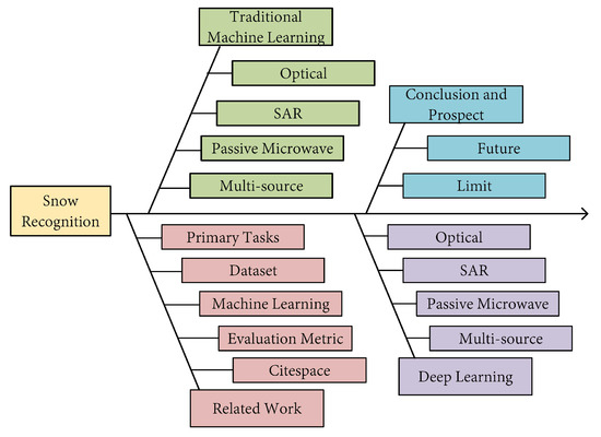
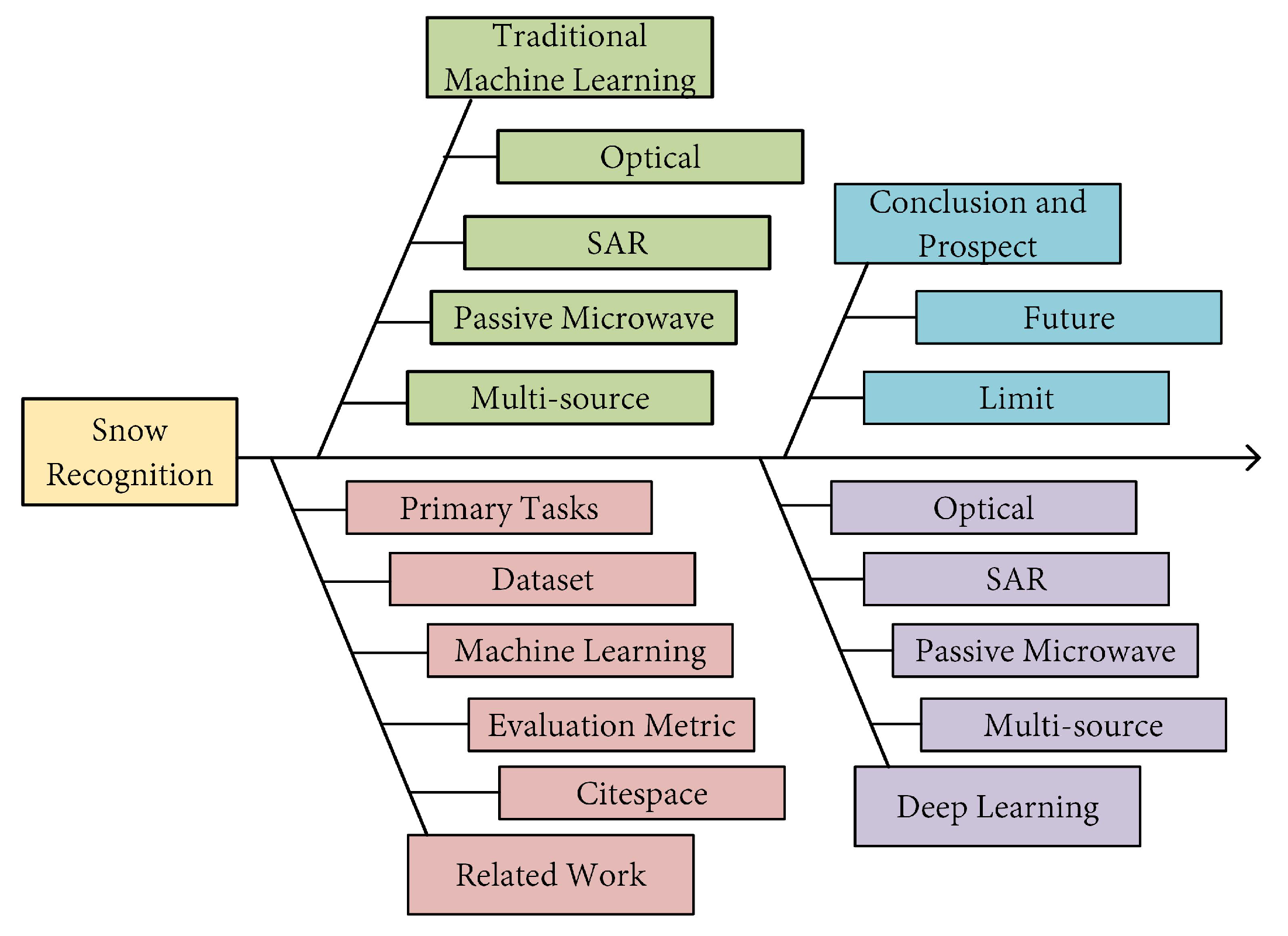
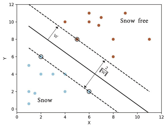
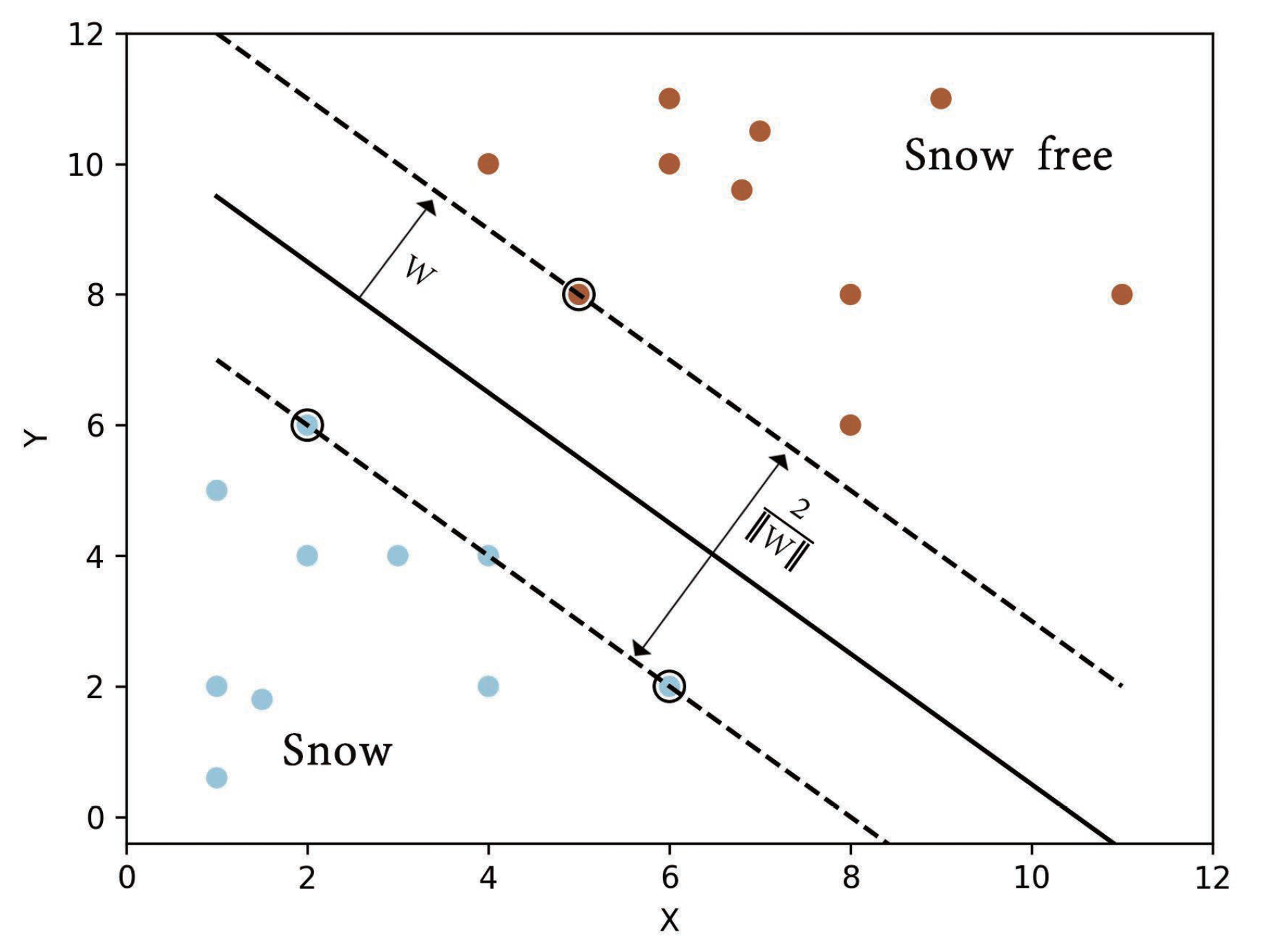
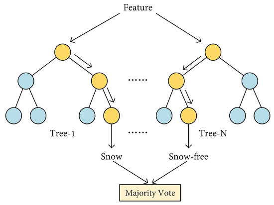
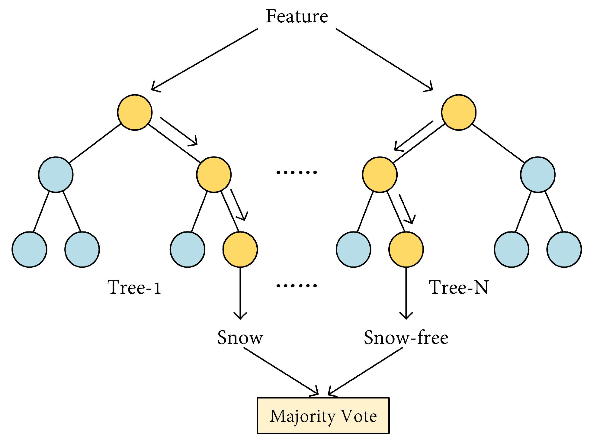
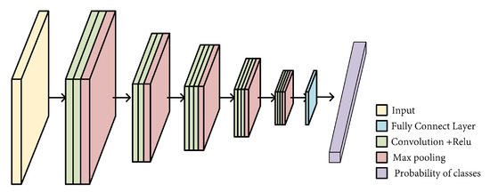
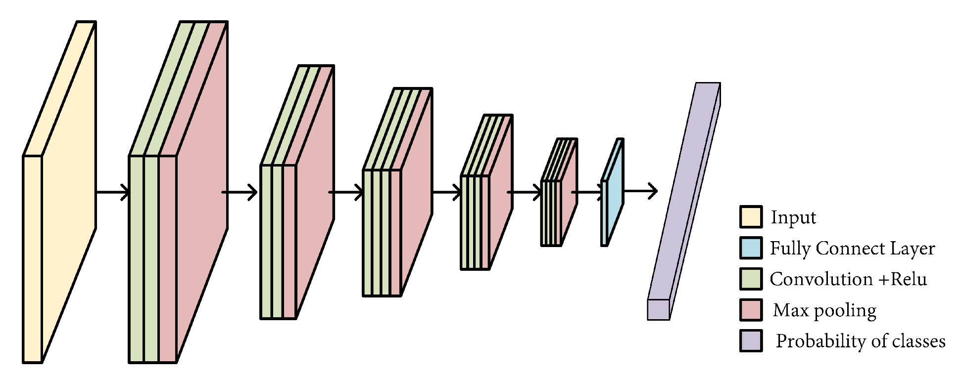
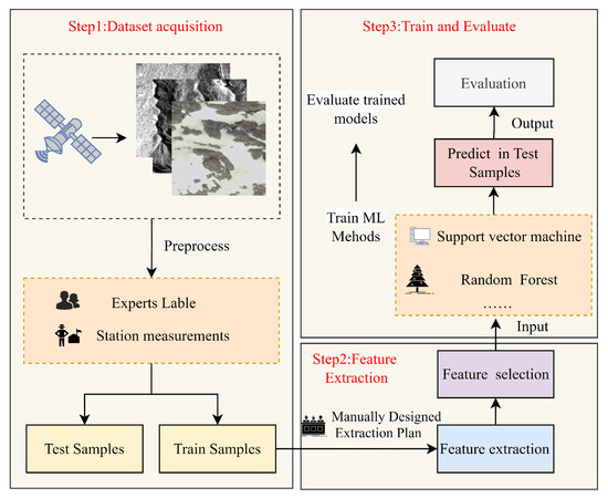
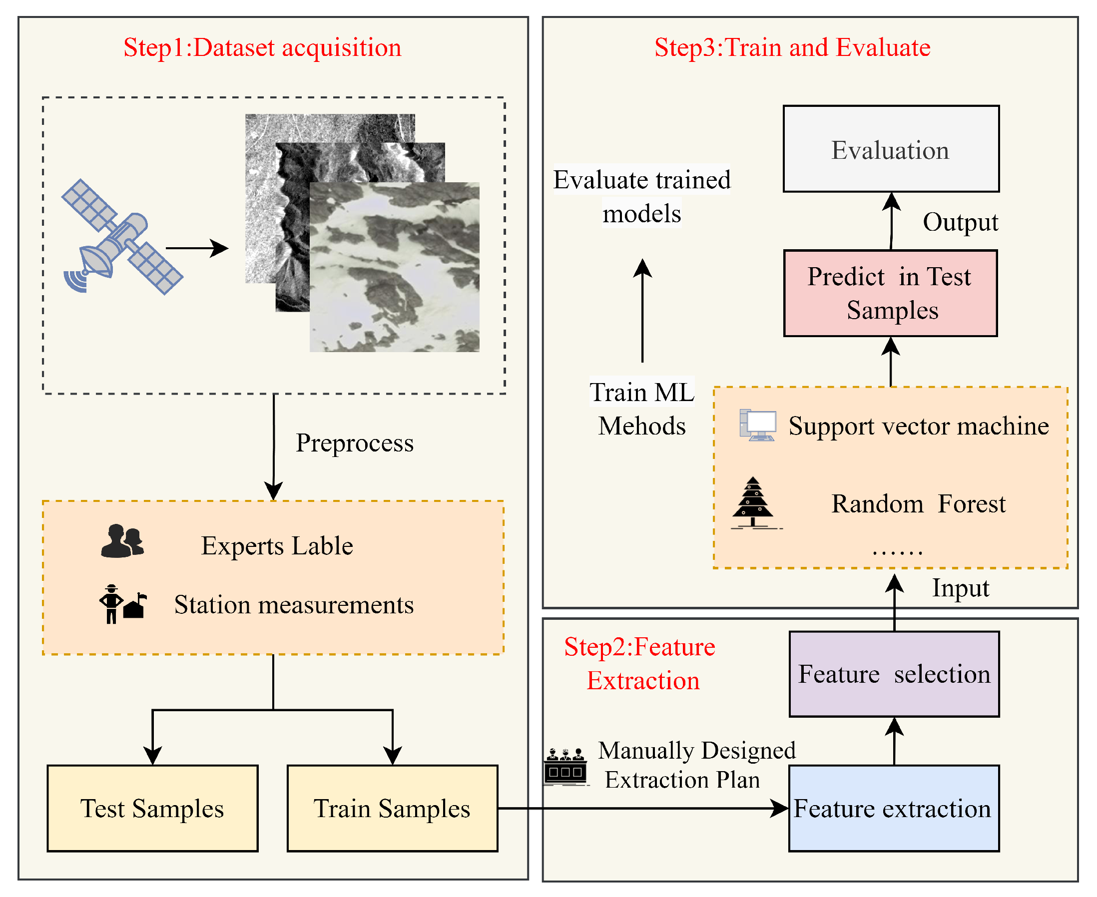
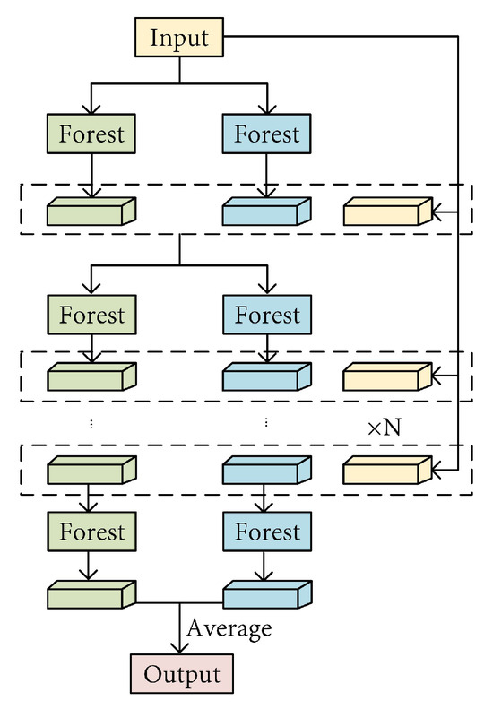
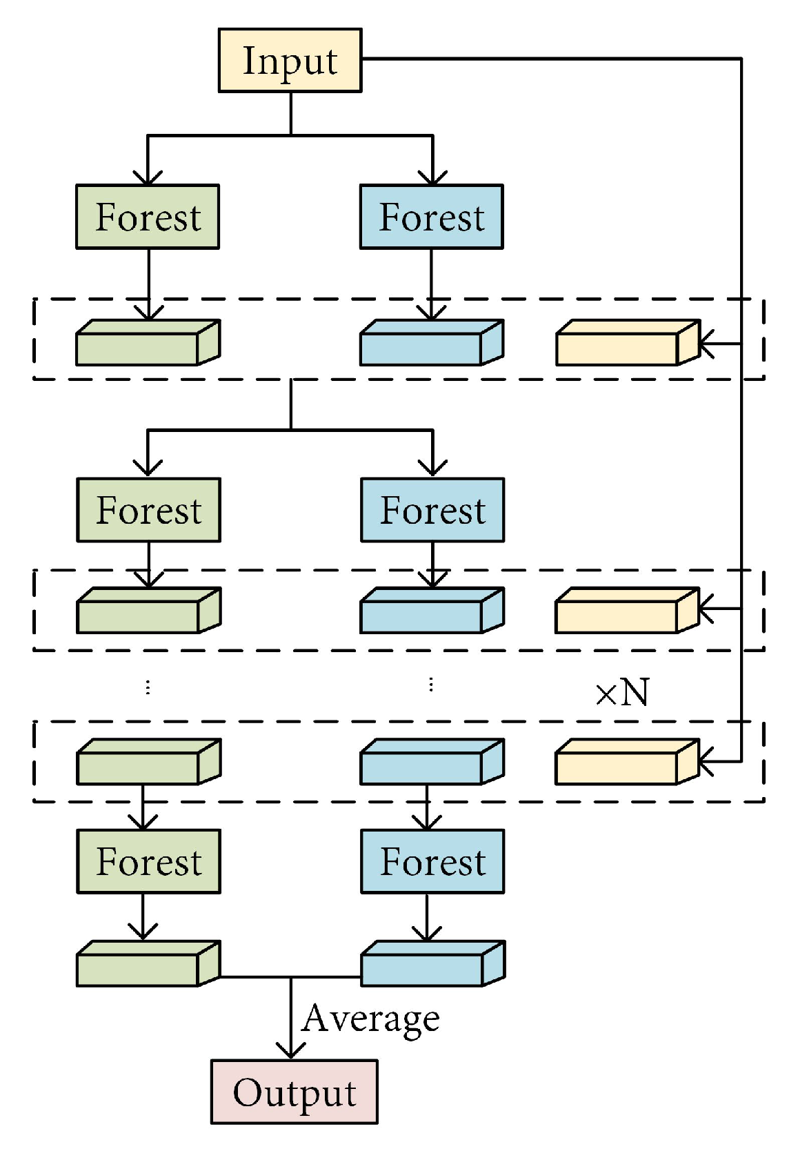
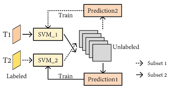
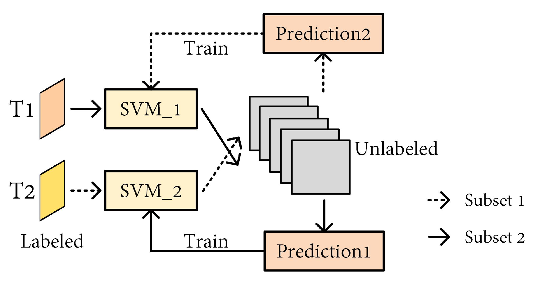
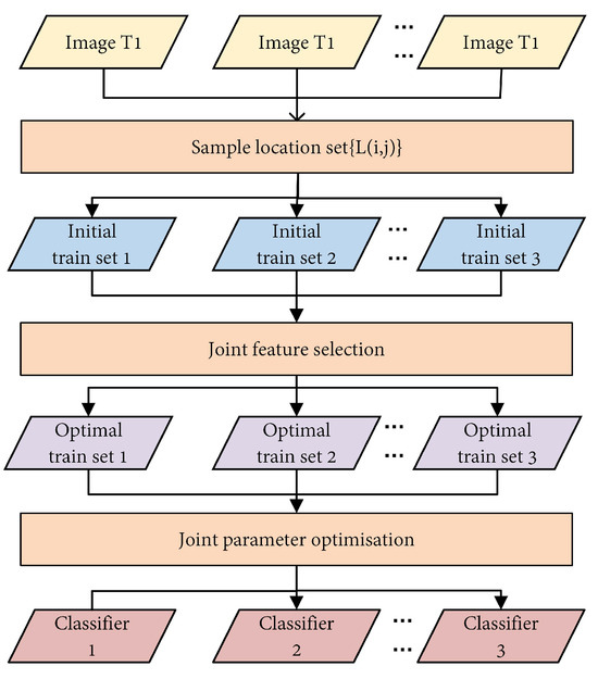
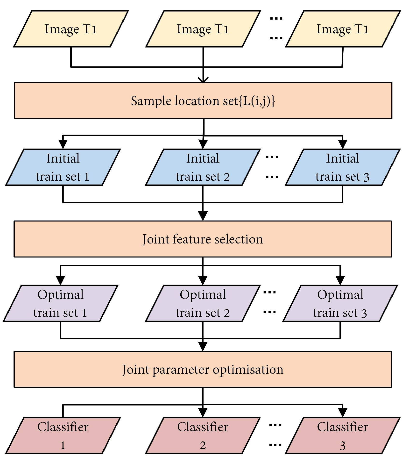
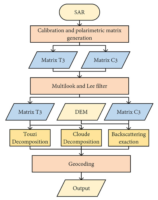
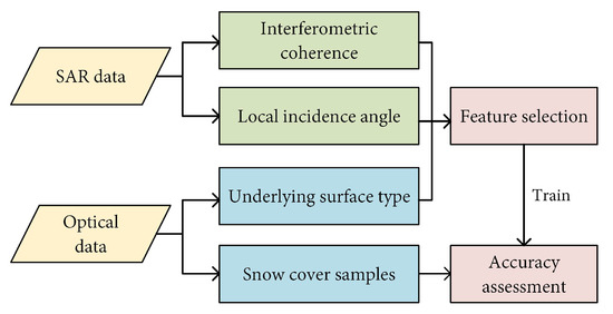
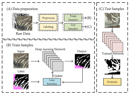
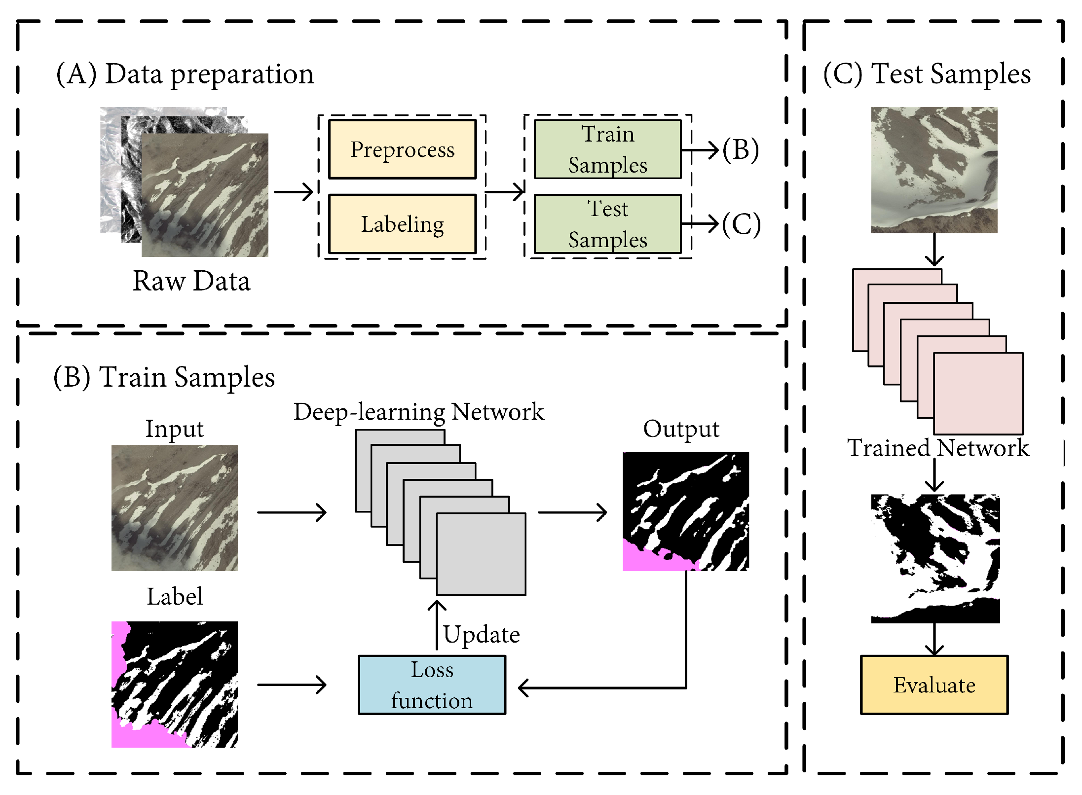
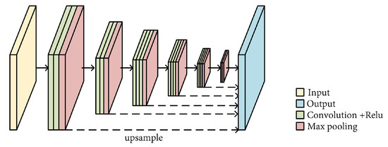
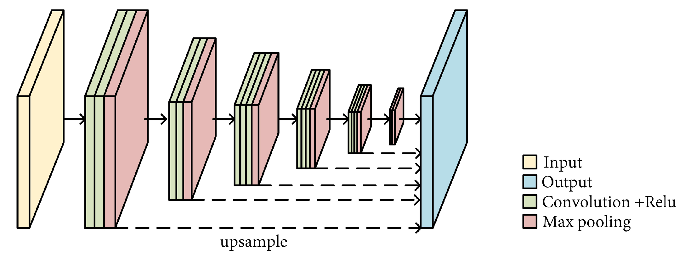
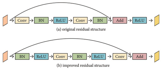
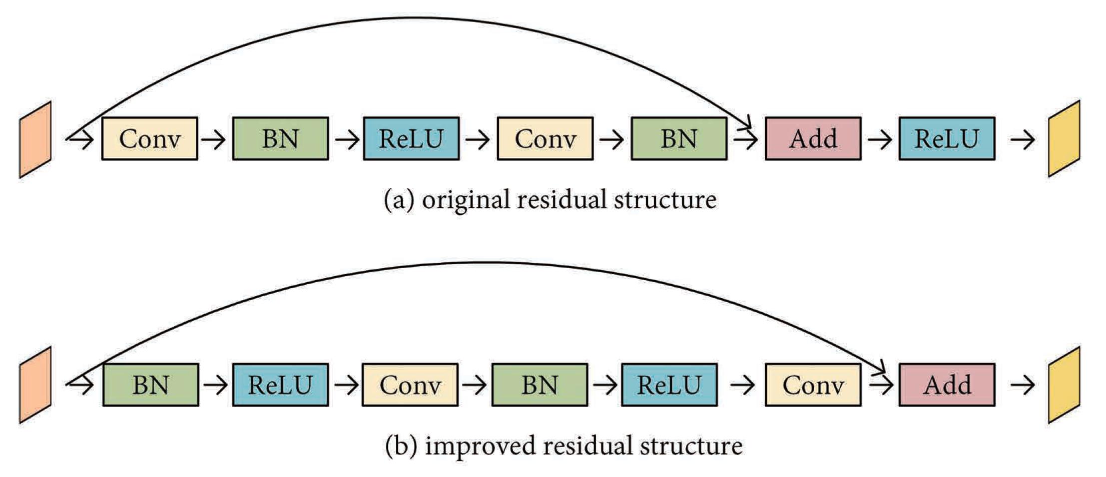
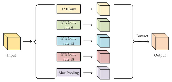
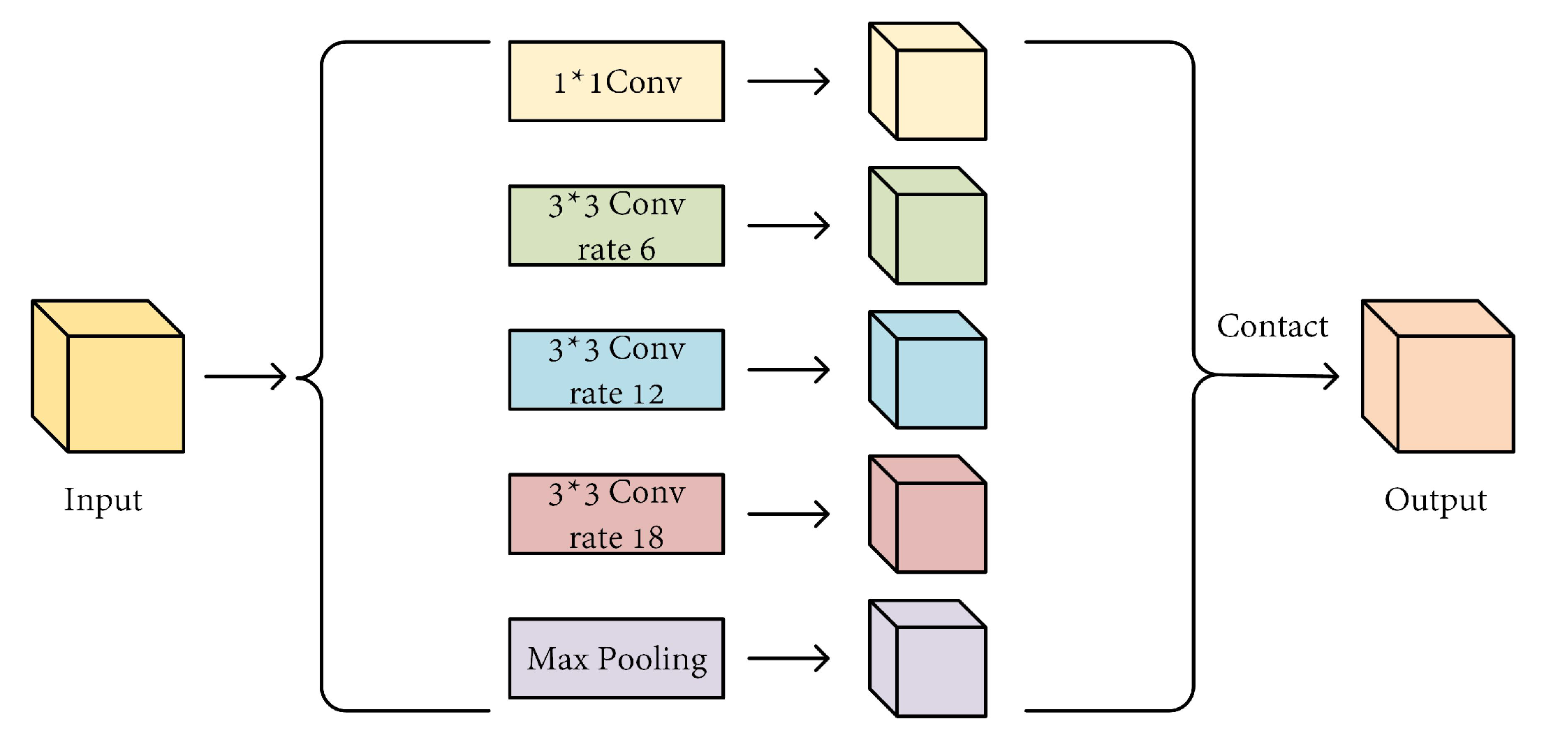
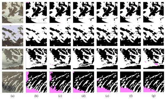
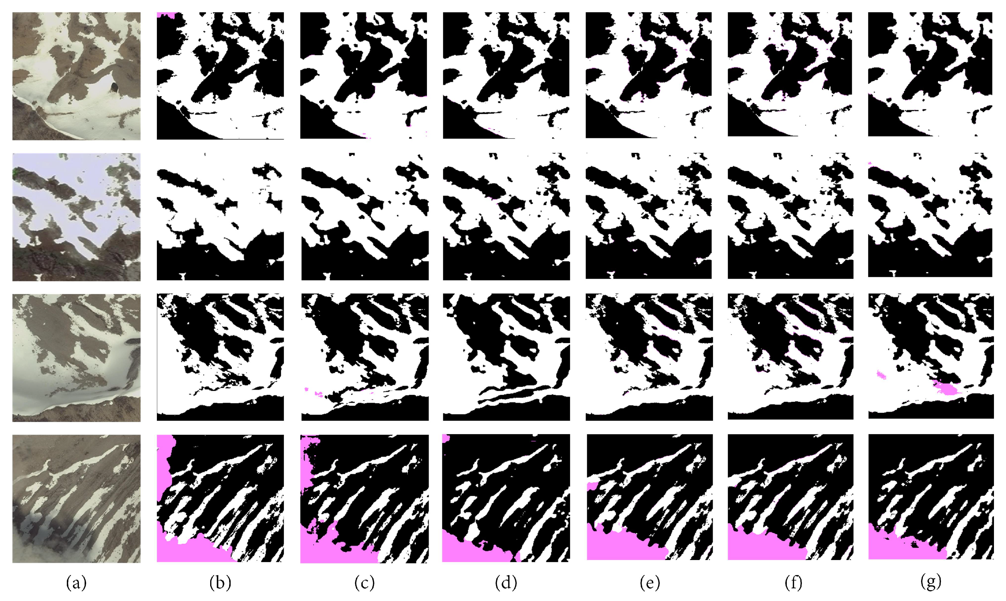
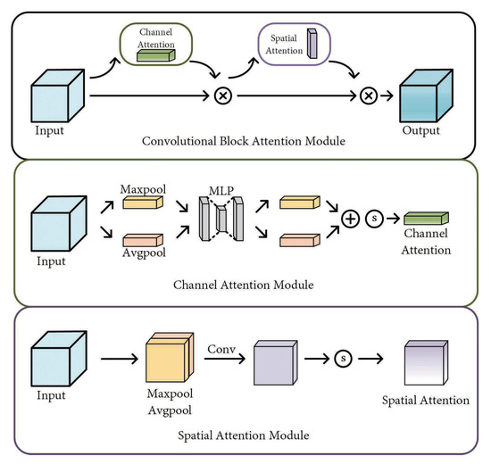
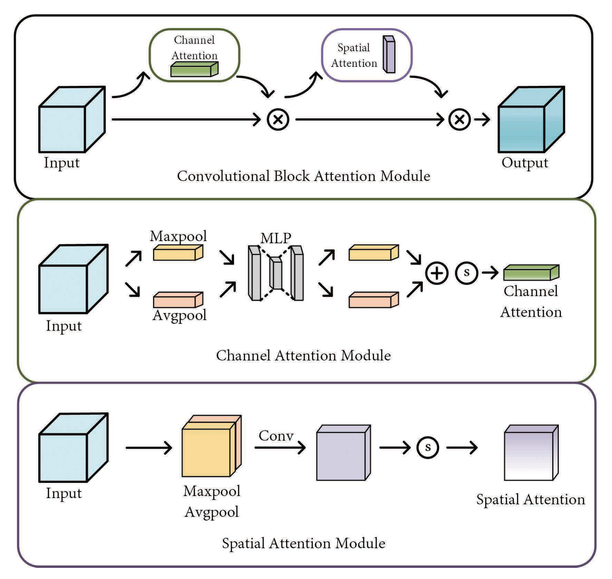
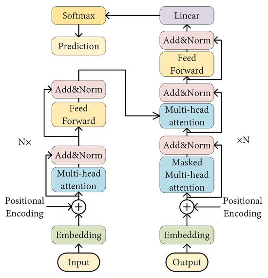
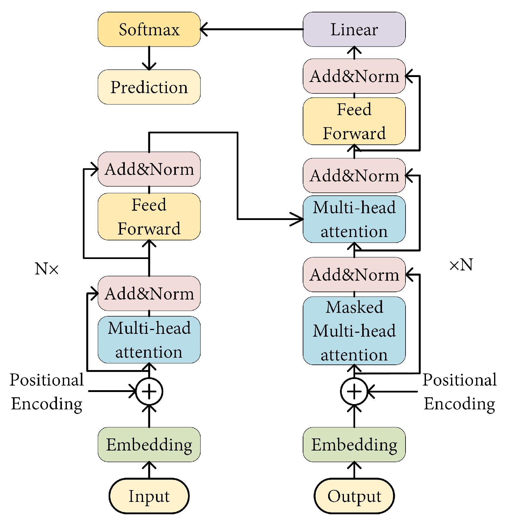
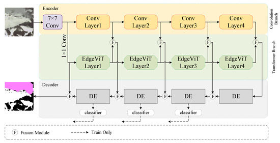
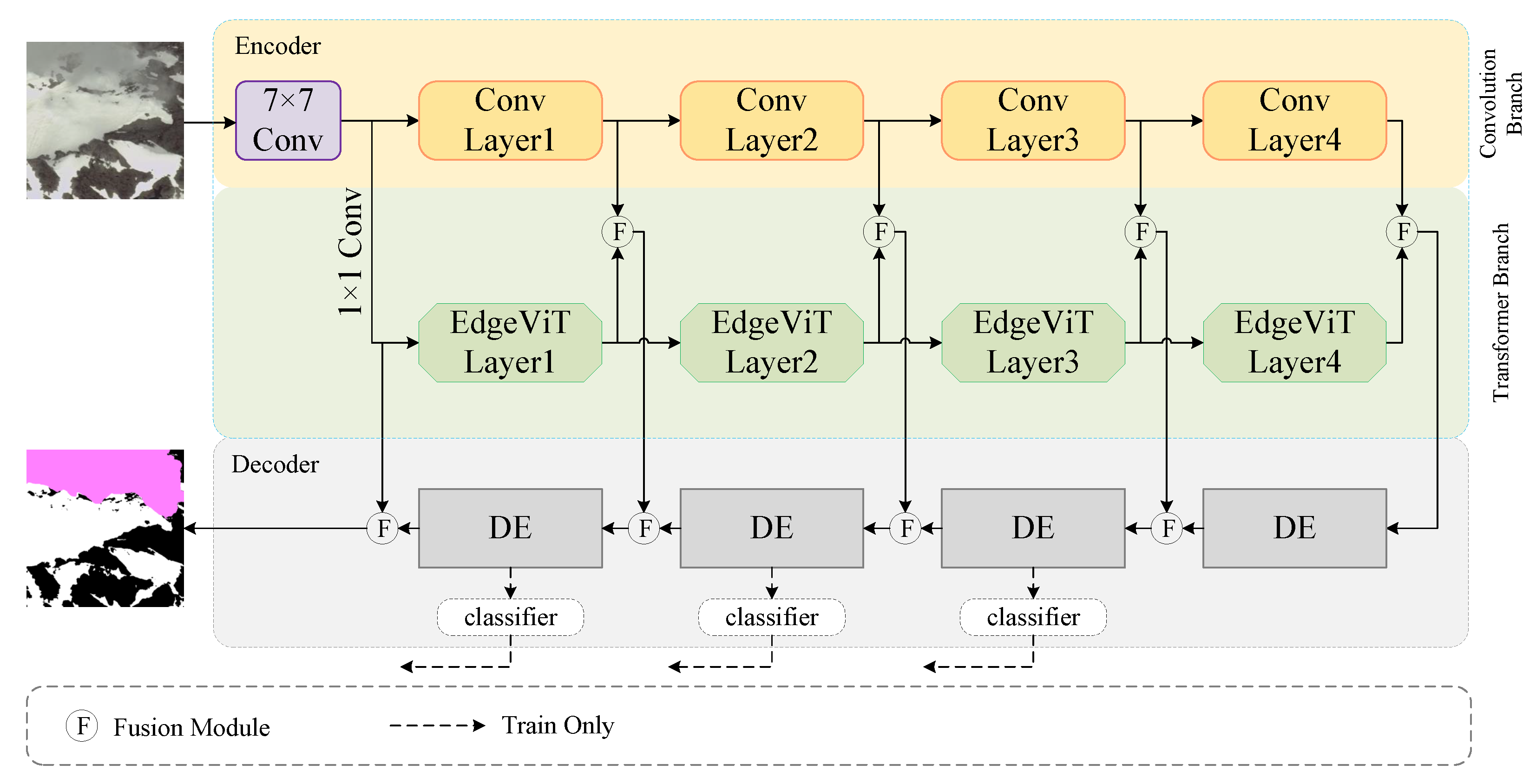

Disclaimer/Publisher’s Note: The statements, opinions and data contained in all publications are solely those of the individual author(s) and contributor(s) and not of MDPI and/or the editor(s). MDPI and/or the editor(s) disclaim responsibility for any injury to people or property resulting from any ideas, methods, instructions or products referred to in the content. |
© 2026 by the authors. Licensee MDPI, Basel, Switzerland. This article is an open access article distributed under the terms and conditions of the Creative Commons Attribution (CC BY) license.