1. Introduction
In the contemporary era of Earth observation, the demand for precise land-cover classification has escalated, driven by the necessity for accurate urban planning, environmental monitoring, and disaster management [
1]. Remote sensing technology has evolved from providing single-modality data to offering a sophisticated array of multi-source information, enabling a more comprehensive understanding of complex terrestrial surfaces [
2]. This shift toward multi-source data integration has proven broadly effective across diverse application scenarios: the fusion of SAR and optical imagery has demonstrated notable gains in land-use classification by exploiting their complementary imaging mechanisms [
3], the joint use of UAV-based multispectral images and LiDAR point clouds has substantially improved urban tree species discrimination [
4], and the integration of heterogeneous multi-temporal observations has advanced land-cover change detection accuracy [
5]. These parallel advances collectively confirm that fusing physically distinct yet complementary data sources consistently yields richer scene representations than any single modality alone. Among these modalities, hyperspectral images simultaneously capture the spatial distribution and detailed spectral reflection information of ground objects [
6], offering rich spectral signatures across hundreds of contiguous bands [
7]. However, HSI data has two limitations: a low spatial resolution hampers the discrimination of spectrally similar materials [
8], and spectral variability causes identical species to exhibit different spectral curves due to environmental factors, while distinct land covers may show similar spectral characteristics in specific wavelength ranges [
9]. To mitigate these challenges, Light Detection and Ranging (LiDAR) has emerged as a critical complementary modality. By providing precise elevation data and spatial geometric information, the elevation characteristics provided by LiDAR alleviate HSI spectral ambiguity [
10], effectively distinguishing between objects that may appear spectrally identical but possess distinct height profiles, such as asphalt roads and tar roofs [
11]. Consequently, the synergistic integration of HSI and LiDAR data has become a pivotal strategy in remote sensing for achieving robust and precise land-cover classification.
The evolution of HSI-LiDAR fusion has transitioned through several paradigms, moving from traditional pixel-level stacking to sophisticated deep learning-based feature-level fusion [
12]. Early research primarily utilized machine learning classifiers. Puttonen et al. [
13] fused LiDAR-derived features with hyperspectral features using SVM [
14,
15] for tree species classification. Spatial feature extractors such as morphological profiles [
16], attribute profiles [
17], and extinction profiles [
18] subsequently emerged. Pedergnana et al. [
19] employed extended attribute profiles (EAPs) to extract features from multispectral and LiDAR images, fusing spectral, spatial, and elevation information through stacked vectors classified by RF [
20] and SVM. More advanced fusion techniques appeared with Liao et al. [
21] designing a graph-based generalized feature fusion framework and Hong et al. [
22] building specialized feature spaces using local preserving projection and linear graph embedding to process concatenated HSI and LiDAR vectors. While these methods established the foundational utility of multimodal data, traditional methods encountered three fundamental challenges that limited their effectiveness: manually designed features depended on subjective assumptions that often failed to transfer across different datasets, shallow learning models could not capture complex nonlinear relationships present in remote sensing data, and a heavy reliance on prior knowledge constrained both classification accuracy and method robustness. These limitations motivated the shift toward deep learning approaches capable of automatic hierarchical feature extraction. With the development of deep learning, significant progress has been made in deep multimodal learning [
23], and convolutional neural networks (CNNs) have become standard for feature extraction [
24].
Convolutional neural networks (CNNs) have transformed remote sensing image analysis through end-to-end learning [
25,
26]. Early CNN designs processed either 1D spectral sequences [
27] or 2D spatial patterns from PCA-reduced data [
28], then evolved to dual-branch 1D/2D networks combining both dimensions [
29]. Chen et al. [
30] introduced 3D CNNs that directly extract joint spatial–spectral features from raw HSI data. He et al. [
31] proposed residual architectures that maintain gradient flow and preserve information across network depth. Zhong et al. [
32] built a spatial–spectral residual network for HSI classification, while Chen et al. [
33] proposed a local–global feature extraction network equipped with dynamic three-dimensional convolution and a residual attention transformer (LGDRNet). For multimodal classification, Hong et al. [
34] developed a deep encoder–decoder network for pixel-level feature extraction from both HSI and LiDAR. Xu et al. [
35] proposed a dual-branch architecture using 2D/1D convolutions for HSI spatial–spectral features and cascade blocks for LiDAR spatial information. Feng et al. [
36] utilized residual blocks for hierarchical, parallel, multi-scale extraction followed by squeeze-and-excitation-based adaptive fusion. Hang et al. [
37] proposed coupled CNNs with simultaneous feature-level and decision-level fusion, while Wu et al. [
38] introduced a cross-channel reconstruction module for enhanced multimodal fusion [
39]. Zhang et al. [
40] developed an interleaving perception CNN for heterogeneous information integration. Hong et al. [
41] proposed a unified framework, extensively researching multistage and multimodal fusion strategies for comprehensive cross-modal data processing. These frameworks significantly improved classification accuracy by learning hierarchical representations that are more discriminative than hand-crafted features. However, standard convolution uses fixed convolution kernel weights and a grouping structure to process an entire image [
42]. This rigid approach lacks the flexibility to adapt to the irregular spatial distribution and channel correlations that exist in different remote sensing datasets [
43].
Group convolution [
44] emerged as an efficient alternative that partitions input channels into multiple groups and performs convolutions independently within each group. This strategy reduces computational complexity and encourages feature diversity by preventing co-adaptation between all channels. Despite these advancements, existing multimodal deep learning frameworks [
45] frequently suffer from two intrinsic limitations that hinder their performance in complex scenarios. First, most conventional CNN-based extractors rely on rigid feature extraction protocols. The group convolution method relies on manually designed channel partition schemes, which introduce additional hyperparameters such as group size and connection mode. These fixed grouping strategies lack flexibility and are unable to adapt to datasets with different spectral and spatial characteristics. Second, there is a notable underutilization of LiDAR-derived textural information. Many models treat LiDAR data merely as a single-channel elevation map, ignoring the fine-grained surface textural details—such as roughness and structural patterns—that are critical for distinguishing objects with similar altitudes.
Recent research has attempted to address these gaps through the introduction of attention mechanisms and adaptive modules. For example, Mohla et al. [
46] introduced FusAtNet, employing self-attention for HSI spectral features and cross-attention-derived masks to enhance HSI spatial features with LiDAR data. Li et al. [
47] proposed TSDN featuring 3D cross-attention blocks for spatial complementarity extraction. Wang et al. [
48] developed MAHiDFNet with a triple-branch CNN backbone and modality attention module for feature interaction. Attention-based architectures have significantly improved feature representation. Because Dosovitskiy et al. [
49] achieved remarkable success by applying the transformer to image classification, researchers began to conduct classification studies, using converters to integrate hyperspectral and radar–laser data. Zhao et al. [
50] integrated convolutional and transformer structures for global–local feature extraction. Ma et al. [
51] proposed a multi-level and multimodal fusion scheme named FTransUNet, aiming to integrate CNN and Vit into a unified fusion framework, providing a robust and efficient multimodal fusion backbone. Roy et al. [
52] proposed a multimodal fusion transformer (MFT) network treating LiDAR data as learnable tokens performing feature learning alongside HSI tokens.
Concurrently, foundation model paradigms have begun to penetrate the HSI domain: Hypersigma scales vision transformers to large-scale hyperspectral pretraining, demonstrating that foundation-level representations can substantially generalize across diverse land-cover scenarios. At the single-modality level, the CSIL framework [
53] addresses the geometric rigidity of fixed-patch inputs by hierarchically sampling center, neighbor, and surrounding regions, thereby enabling multi-grained spatial interaction mechanisms that better characterize the varying scales of land-cover types. For the multimodal setting, THSGR [
54] proposes a heterogeneous graph encoder coupled with a self-attention–free multi-convolutional modulator, explicitly constructing salient topological relationships across modalities while mitigating the redundancy and overfitting issues inherent in standard transformer-based fusion.
However, the high computational complexity of standard transformers and their relative weakness in capturing local spatial contexts remain significant hurdles. Furthermore, while some adaptive grouping strategies have been explored in computer vision, their application to the specific high-dimensional and heterogeneous nature of HSI-LiDAR data remains underexplored. Current fusion strategies also tend to introduce modality imbalance. The fusion mechanisms in many current models are often asymmetric or unidirectional. Common strategies fail to balance the contributions of spectral and elevation features effectively, often leading to a “modality collapse”, where the network over-relies on the dominant HSI signals and treats LiDAR as a secondary, less influential input. The fixed grouping strategy lacks flexibility and is unable to adapt to the problems of datasets with different spectral and spatial characteristics. This issue remains unsolved. It is also worth noting that while advanced HSI-centric models, such as the Enhanced Multi-Scale Feature Fusion Network (EMFFN) [
55], have demonstrated strong performance by employing parallel multipath structures to capture multi-scale spectral–spatial features within a single modality, their fixed convolutional kernels and single-modality design orientation leave them ill-suited for heterogeneous HSI-LiDAR scenarios. In multimodal contexts, rigid feature extraction protocols cannot accommodate the irregular spatial–spectral distributions that arise from fusing physically distinct data sources, nor do they provide mechanisms for balanced cross-modal interaction. These differences led us to make certain core design choices for the framework: replacing fixed-kernel convolutions with dynamically learned channel groupings and substituting unidirectional hierarchical aggregation with a bidirectional cross-attention mechanism that enforces mutual guidance between spectral signatures and LiDAR-derived elevation textures.
To address these challenges, this paper proposes a novel framework named DGC-BCAF, which integrates Dynamic Group Convolution and Bidirectional Guided Cross-Attention to achieve adaptive feature representation and robust cross-modal interaction. The DGC-BCAF architecture is designed to move beyond the “one-size-fits-all” approach of traditional fusion networks. First, we introduce a Dynamic Group Convolution (DGConv) module embedded within a ResNet18 backbone. Unlike traditional group convolution, which uses a fixed number of groups, this module learns a dynamic relationship matrix to automatically group input channels. This allows the network to facilitate flexible, context-aware feature representation that adapts to complex spatial–spectral distributions. Second, to overcome the insufficient exploitation of elevation data, we design a dedicated LiDAR texture encoding branch. This branch innovatively fuses Gray-Level Co-occurrence Matrix (GLCM) statistical features with multi-scale convolutional representations, capturing both macro-level geometric height and micro-level surface textural details. Finally, at the heart of our architecture is the Bidirectional Cross-Attention Fusion (BCAF) module. Unlike standard unidirectional approaches, BCAF employs a LiDAR geometry to guide the selection of salient spectral bands while simultaneously utilizing spectral signatures to emphasize informative LiDAR channels. This mutual guidance ensures a balanced and optimized contribution from both modalities, leading to superior classification performance.
The main contributions of this study are summarized as follows:
We propose the DGC-BCAF framework, a novel end-to-end deep learning architecture that achieves state-of-the-art performance in HSI-LiDAR joint classification by emphasizing Adaptive Feature Extraction and bidirectional modality interaction.
We design a Dynamic Group Convolution (DGConv) module based on a learnable relationship matrix. This module enhances the flexibility of the ResNet18 backbone, allowing it to adaptively group channels and extract more discriminative spatial–spectral features compared to rigid, fixed-structure convolutions.
We introduce a comprehensive LiDAR texture encoding branch that integrates GLCM-based statistical descriptors with multi-scale CNN features. This dual-path approach ensures that the structural and textural nuances of the elevation data are fully preserved and utilized.
We develop a Bidirectional Cross-Attention Fusion (BCAF) mechanism that facilitates mutual guidance between HSI and LiDAR. By enabling reciprocal feature refinement, the model effectively addresses the modality imbalance problem and improves the delineation of spectrally similar materials in complex urban structures.
The effectiveness of the proposed DGC-BCAF is rigorously evaluated on three widely recognized benchmark datasets: Houston 2013, Trento, and MUUFL. Experimental results demonstrate that our method consistently outperforms existing state-of-the-art approaches in terms of overall accuracy (OA), average accuracy (AA), and Kappa coefficient.
2. Proposed Method
In this section, a network termed dynamic grouped convolution and Bidirectional Guided Cross-Attention collaborative training (DGC-BCAF) is presented in detail. The basic definitions and symbol descriptions are introduced first. The overall architecture of the proposed framework is then outlined to clarify its structural design and functional components. Then, the main components of the proposed network are elaborated, including the dynamic grouping convolution module, the self-attention encoder module, the Bidirectional Cross-Attention Fusion module, and the feature fusion classification module integration. Finally, the training strategies are discussed and the algorithm structure is presented.
2.1. Overall Framework of the Proposed Method
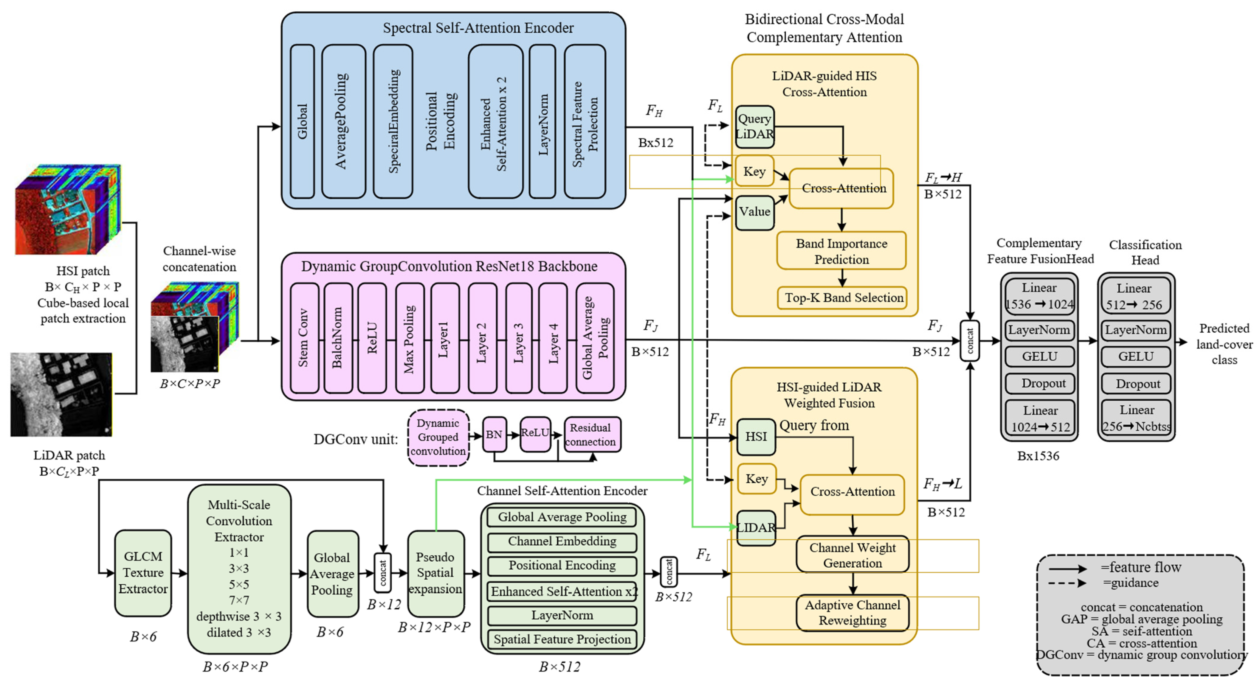
To provide a clear and coherent understanding of the proposed DGC-BCAF network, we present a high-level overview of the complete feature flow, as illustrated in
Figure 1. The DGC-BCAF framework is designed to fully exploit the complementary information from hyperspectral imagery (HSI) and LiDAR data for accurate land-cover classification. The overall process can be summarized as follows:
First, for each pixel, we extract local cube-based patches from both the HSI and LiDAR data. The HSI patch is processed by a Spectral Self-Attention Encoder, which captures discriminative spectral features and contextual dependencies among spectral bands. Simultaneously, the LiDAR patch is fed into a GLCM-based texture extractor and a multi-scale convolutional module to obtain both texture and spatial–geometric features. These LiDAR features are then encoded by a Channel Self-Attention Encoder to enhance spatial representation.
The extracted HSI and LiDAR features are then passed through two symmetric, bidirectional cross-attention modules: (1) a LiDAR-guided HSI cross-attention module, which adaptively selects the most informative HSI spectral bands based on LiDAR cues, and (2) an HSI-guided LiDAR fusion module, which generates adaptive weights for LiDAR channels using HSI features. This bidirectional interaction enables mutual refinement and robust feature selection across modalities.
In parallel, the original HSI and LiDAR data are concatenated and processed by a dynamic grouped convolutional ResNet backbone, which further extracts joint spectral–spatial representations. Finally, the outputs from the ResNet backbone, the LiDAR-guided HSI module, and the HSI-guided LiDAR module are concatenated and fused through a complementary feature fusion module, followed by the final classification layer.
This end-to-end architecture ensures that both spectral and spatial–geometric information is fully leveraged and interactively refined at multiple stages, resulting in improved classification performance and generalization.
Mathematically, given an HSI dataset, , and its corresponding LiDAR dataset, , where H and W denote the spatial height and width of both datasets, refers to the total number of bands available in the hyperspectral data, and represents the number of channels in the LiDAR data. For the pixel, we extract cube-based patches denoted as and , where is the spatial patch size.
2.1.1. The Dynamic Group Convolution Module Based on ResNet18
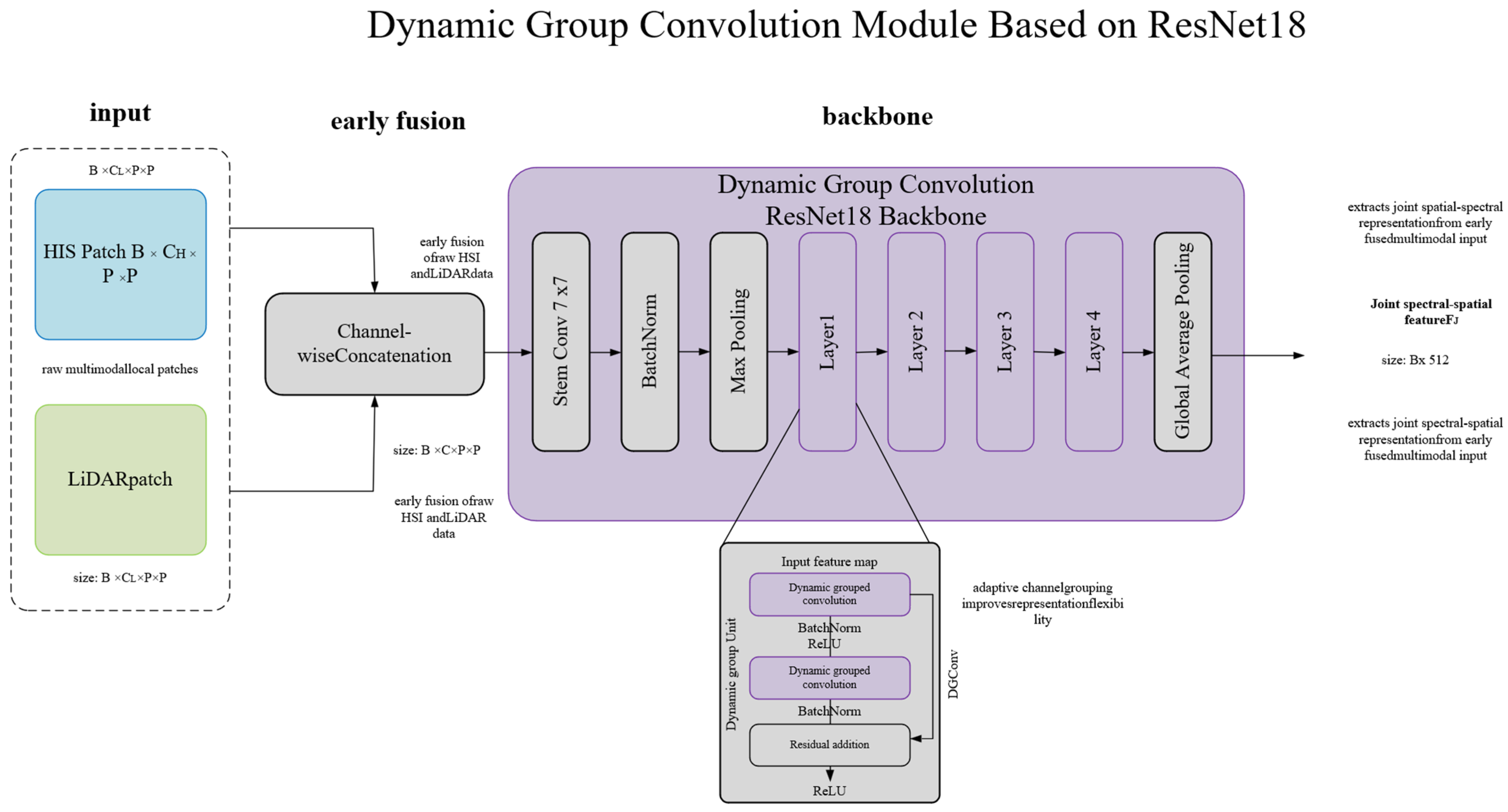
The Dynamic Group Convolution (DGConv) unit is described here.
Figure 2 presents how DGConv is incorporated within the ResNet18 backbone. The DGConv module is designed to enhance the flexibility and representation capability of conventional group convolution by adaptively learning the channel relationships, thereby enabling more effective feature extraction for remote sensing image classification.
2.1.2. Definition of Dynamic Group Convolution
Let
denote the input feature map, where
is the number of input channels and H and W are the spatial dimensions. The output feature map is denoted as
, where
is the number of output channels. The DGConv operation is formally defined as follows:
where
represents the convolution kernel at spatial location,
is a learnable binary relationship matrix, and
denotes element-wise multiplication. The matrix U determines which input channels contribute to each output channel, thus enabling dynamic channel grouping. This formulation generalizes several conventional convolution operations. For example, when U is a matrix of ones, DGConv reduces to standard convolution. If U is an identity matrix, DGConv becomes depthwise convolution. Furthermore, a block-diagonal structure in U corresponds to traditional group convolution.
2.1.3. Learning the Relationship Matrix U
Directly learning the binary matrix U is challenging due to the discrete nature of its elements and the large number of parameters involved. To address these issues, we decompose U into a set of smaller matrices and introduce a learnable gate vector to generate U efficiently.
Assume
, where K is an integer. We define a set of K small matrices,
, each of size
, and reconstruct U via the Kronecker product:
where
denotes a Kronecker product. Each small matrix
is parameterized by a binary gate
:
where
is a
matrix of ones and
is the
identity matrix. Thus, the full relationship matrix U can be constructed from a gate vector,
, significantly reducing the number of learnable parameters. To enable gradient-based optimization, we relax the binary constraint by introducing a continuous gate vector,
, and obtain the binary gates via the sign function:
Combining the above, the relationship matrix U is constructed as follows:
During training, the non-differentiable sign function is approximated by the straight-through estimator. This strategy enables backpropagation to proceed normally and allows model parameters to be updated effectively.
2.1.4. Early Feature Fusion of Dual Modalities
The initial stage of our framework involves the integration of two distinct modalities, denoted as
and
. To preserve the raw spatial–spectral correlations from the outset, we employ an early fusion strategy via channel-wise concatenation. This process is formulated as follows:
2.1.5. Integration into ResNet18
To utilize DGConv in the backbone network, the standard convolutional layers in ResNet18 are replaced with DGConv layers. In each residual block, convolution operations are implemented through DGConv, which allows channels to be grouped dynamically and features to be extracted in an adaptive manner. As a result, the residual block is reformulated as follows:
where
and
denote the input and output feature maps,
and
are Dynamic Group Convolution layers,
and
are batch normalization layers, and
is the residual connection. This integration allows the network to adaptively learn channel relationships at each layer, improving its ability to capture complex spatial–spectral patterns in remote sensing data.
We embed the DGConv module within the standard blocks of ResNet18. The layer channel count determines the group number and the gate vector length, K. The structure keeps the depth and links of the original ResNet18 intact. Dynamic Group Convolution groups channels as needed. This helps the ResNet18 backbone find features. A learnable matrix adjusts the receptive fields.
The final output of this module is the cross-modal joint feature map, denoted as
:
2.2. Self-Attention Encoder Module
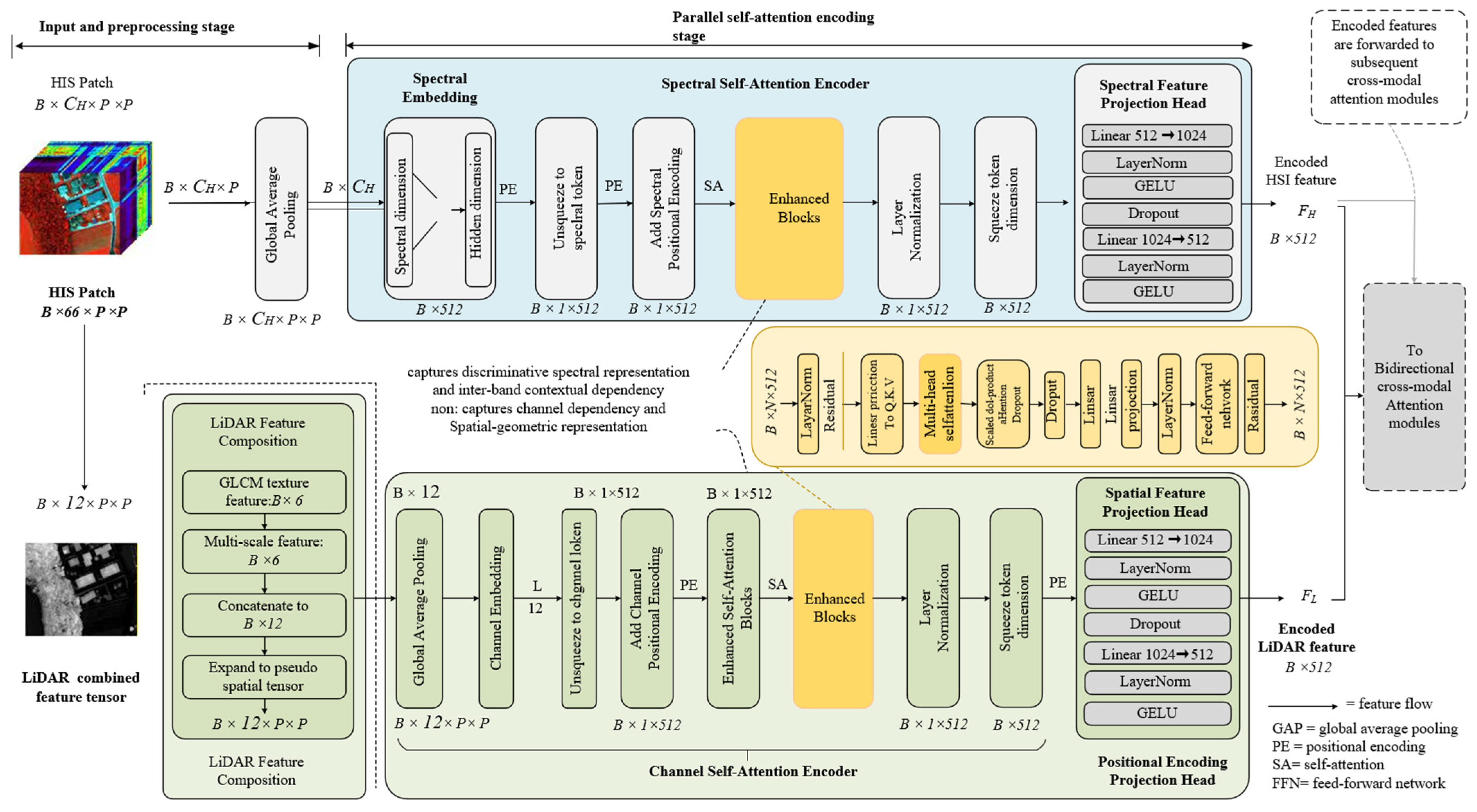
As illustrated in
Figure 3, the self-attention encoder module receives inputs from hyperspectral images (HSI) and LiDAR sources. The goal is to obtain clear features from the raw data. This structure divides into two parallel paths. We use the Spectral Self-Attention Encoder to process HSI data. The Channel Self-Attention Encoder handles the LiDAR input. Each path uses a self-attention block. This method helps the network find links between distant points. It also gathers details about the surroundings in each data type.
2.2.1. Spectral Self-Attention Encoder for HSI
The Spectral Self-Attention Encoder is specifically designed to utilize the spectral characteristics present in HSI data. For an input HSI patch,
, where
is the number of spectral bands, global average pooling is first applied to generate a concise spectral representation:
where GAP refers to adaptive average pooling across spatial dimensions. The resulting spectral vector is then mapped to a higher-dimensional embedding space using a linear transformation:
In this equation, and are learnable parameters. To incorporate positional information, a spectral positional encoding, , is added, where D is the embedding dimension.
The spectral features are subsequently processed through
layers of the self-attention block. Each layer includes a multi-head self-attention (MSA) operation, followed by a feed-forward network (FFN). Both components use residual connections and layer normalization:
The self-attention mechanism calculates attention weights for each input embedding
by projecting the query, key, and value matrices through linear transformations:
where
is a learnable weight matrix. The attention scores are computed using scaled dot-product attention:
where
is the dimension of each attention head. The output of the self-attention block is then
Then, the output of the multi-head self-attention is
where
is the projection matrix. After passing through all the attention layers, the final spectral feature is extracted via an MLP network:
where
represents the encoded spectral feature.
2.2.2. Channel Self-Attention Encoder for LiDAR
The Channel Self-Attention Encoder processes LiDAR-derived features by explicitly modeling dependencies among texture and multi-scale spatial representations. The input to this encoder consists of concatenated GLCM texture features and multi-scale geometric features, forming a 12-channel representation , where .
Prior to attention encoding, we extract GLCM texture features from the original LiDAR intensity data. The GLCM is computed by quantizing the intensity values into G = 16 gray levels and calculating co-occurrence statistics at specified distances, d, and angles, θ. For a quantized patch, the GLCM matrix,
, represents the joint probability of gray-level pairs:
From the normalized GLCM, six texture descriptors are derived to characterize surface roughness and structural patterns.
Contrast quantifies local intensity variations:
Correlation measures gray-tone linear dependencies:
Energy (angular second moment) reflects texture uniformity:
Homogeneity emphasizes diagonal elements, indicating smoothness:
Entropy captures randomness in texture:
Variance describes gray-level dispersion:
Six texture descriptors are grouped together by channel. The result is a GLCM feature vector:
We extracted the above six texture features using the GLCM method. In order to construct a more comprehensive subset of LiDAR data features, we extracted the following six-dimensional multi-scale features through the deep learning CNN method:
Fine-grained point-based feature extraction: Using 1 × 1 convolution kernels to capture pixel-level local features, this operation is equivalent to performing independent nonlinear transformations for each spatial position:
Local neighborhood feature extraction: Convolution is the most commonly used basic unit in computer vision, which can effectively capture the local neighborhood information of pixels:
Extraction of structural features of medium-scale structures: The convolution kernel expands the receptive field range and is capable of capturing structural information at medium scales:
Large-scale global context extraction: Use large-scale convolution kernels to capture broader spatial context information:
Depthwise Separable Convolution splits regular convolution into channel-wise filtering and per-pixel transformation. This method extracts spatial information from each channel. Model parameters are reduced:
Expanding convolution multi-scale context aggregation: The expansion convolution (also known as the dilated convolution) exponentially expands the receptive field without increasing the number of parameters by introducing a dilation rate of
:
where
represents a standard convolution operation with kernel size
. Depthwise convolution,
, applies a 3 × 3 kernel and group convolution. The calculation load drops. Local feature extraction works well. Dilated convolution,
, sets a dilation rate of 2. The receptive field widens. The parameter count does not rise.
Six feature maps represent height data at different levels. The convolution keeps specific point details. The and kernels focus on the nearby area. The kernel covers a wider background. Depthwise convolution handles spatial links. Dilated convolution finds connections between distant parts. We join these outputs along the channel axis:
The multi-scale convolutional features,
, and GLCM texture features,
, provide complementary information. To effectively fuse the multi-scale convolutional features and the GLCM texture features, it is necessary to ensure that both feature sets have compatible spatial dimensions. The convolutional features inherently possess spatial dimensions corresponding to the input image (H × W), whereas the GLCM features are typically computed as global or local statistical descriptors and may lack explicit spatial structure. To address this, we spatially broadcast the GLCM features across the entire image domain. Specifically, as shown in the formula below:
Each GLCM feature channel is repeated along the spatial dimensions (H and W), resulting in a tensor, , that matches the shape of the convolutional features. Here, the operation replicates each of the six GLCM feature channels uniformly across all spatial locations. This broadcasting enables the subsequent integration of the GLCM texture descriptors with the convolutional features, facilitating joint learning and improved representation of both hierarchical and statistical texture information.
The 6-dimensional texture descriptors and 6-dimensional multi-level features are merged across the channel axis. This process yields a full LiDAR feature set, as shown below:
The spectral encoder uses this operation. Global mean pooling is used here to collect spatial features:
A linear embedding layer projects these descriptors into the latent space. A learnable channel positional encoding
is added:
The embedded channel features are processed through
layers of the self-attention block:
Self-attention is applied within this pathway. Its operation follows the same process as used for the spectral pathway. This design allows the network to capture dependencies between channels and spatial patterns. The channel representation is then obtained using a multi-layer perceptron:
where
denotes the encoded LiDAR feature.
2.3. Bidirectional Cross-Attention Fusion Module
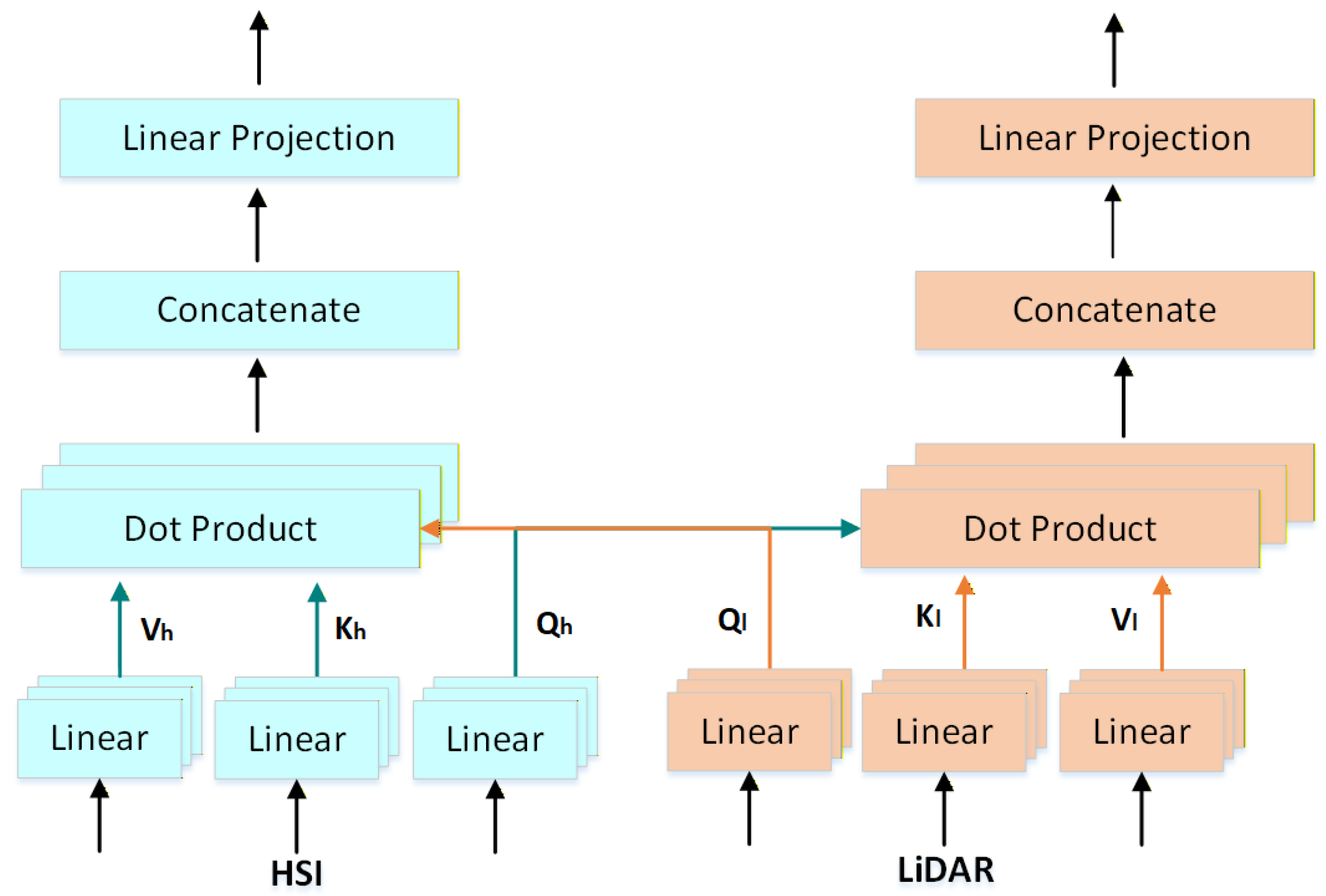
In this section, we introduce a Bidirectional Cross-Attention Fusion mechanism designed to facilitate the mutual guidance and optimization of hyperspectral (HSI) and LiDAR features. This module consists of two complementary submodules: (1) LiDAR-guided hyperspectral band selection and (2) hyperspectral-guided LiDAR channel optimization. Both submodules operate on the outputs of the preceding self-attention encoder modules, enabling fine-grained feature interaction and selection, as shown in
Figure 4.
2.3.1. LiDAR-Guided Hyperspectral Band Selection
The initial submodule uses spatial cues from LiDAR data to identify valuable hyperspectral bands. Modeling cross-modal association involves applying a cross-attention module with multiple heads. LiDAR features function as queries. Hyperspectral features correspond to keys and values.
LiDAR features undergo projection within the attention domain:
Similarly, HSI features are projected to form keys and values:
The cross-attention mechanism computes
where
encodes the LiDAR-guided HSI information.
Unlike previous approaches that rely solely on attention weights, we introduce a learnable band importance predictor to directly estimate the contribution of each spectral band. Specifically, the cross-attention output is passed through a multi-layer perceptron to produce band importance scores:
where
denotes the importance score for the spectral band. The top
bands with the highest scores are selected:
where
is the number of selected bands and
in our implementation.
The selected band features are then aggregated and processed via a feed-forward network to obtain the final fused representation:
where
denotes the selected band processor.
2.3.2. HSI-Guided LiDAR Channel Weighted Fusion
The second module utilizes hyperspectral features to adaptively weight and optimize LiDAR channel representations. Texture information and spatial features at different scales are obtained. These features are merged together. This process produces a unified LiDAR feature matrix.
First, HSI features are projected into the attention space:
Similarly, LiDAR features are projected to form keys and values:
The cross-attention mechanism computes
where
encodes the HSI-guided LiDAR information.
The result from cross-attention helps assign variable importance to every LiDAR channel. Each channel receives a score that reflects its relevance:
where
and
are learnable parameters.
The original LiDAR channel features are globally pooled:
The weighted fusion is performed via element-wise multiplication and summation:
The fused feature is further processed by a feed-forward network to obtain the final representation:
where
denotes the weighted band processor.
2.4. Complementary Feature Fusion Classification
The fusion module receives three distinct feature representations: (1) the cross-modal features extracted by the dynamic grouped convolution ResNet-18 backbone are used to extract the basic spectral–spatial information, , through adaptive feature learning; (2) the LiDAR-guided cross-attention selects the important HSI band information, ; (3) the HSI-guided cross-attention optimizes the constructed LiDAR feature set information, .
The three feature streams are initially merged across the feature axis. This process yields an integrated representation vector:
where
denotes the concatenation operation. This concatenated representation preserves the complete information from all processing pathways, ensuring that no discriminative features are lost during the initial aggregation stage.
The resulting classification from this procedure is formulated as follows:
The softmax operation maps the fused feature vectors to a set of probabilities, C denotes the categories of ground objects within the dataset, indicates the dense layer, and gives the annotation for pixel i.
2.5. Algorithm
To provide a comprehensive overview of the proposed DGC-BCAF framework, the detailed step-by-step training strategy is presented in this section. The overall procedure encompasses several key stages: initial data patch construction, cross-modal joint feature extraction via the Dynamic Group Convolution (DGC) module, modality-specific feature encoding (including GLCM texture extraction for LiDAR), and the core Bidirectional Cross-Attention Fusion. Finally, the complementary features are integrated to generate the final land-cover classification map. The complete execution flow and the corresponding mathematical implementations are systematically summarized in Algorithm 1.
| Algorithm 1. The overall training strategy of the DGC-BCAF framework is outlined in the algorithm |
| Input:The original HSI and corresponding LiDAR data , . |
| Output:The classification map . |
| 1: Construct small patches and from and , respectively. |
| 2: for do |
| 3: # The Dynamic Group Convolution Module Based On ResNet18 |
| 4: Perform early fusion via channel-wise concatenation of and with Equation (7); |
| 5: Extract cross-modal joint features using DGC-ResNet18 with Equation (9); |
| 6: # Spectral Self-Attention Encoder for HSI; |
| 7: Extract spectral features using self-attention encoder with Equations (10)–(18); |
| 8: # Channel Self-Attention Encoder for LiDAR; |
| 9: Extract GLCM texture feature with Equations (20)–(26); |
| 10: Extract multi-scale spatial features with Equations (27)–(33); |
| 11: Combining texture and multi-scale features to form , and using the channel self-attention encoder to extract LiDAR features with Equations (35)–(40); |
| 12: # LiDAR-Guided Hyperspectral Band Selection; |
| 13: Apply LiDAR-guided cross-attention on to select important HSI spectral bands feature with Equations (41)–(47); |
| 14: # HSI-Guided LiDAR Channel Weighted Fusion; |
| 15: Apply HSI-guided cross-attention to optimize LiDAR feature subset, obtaining weighted band feature with Equations (48)–(55); |
| 16: # Complementary Feature Fusion Classification; |
| 17: Fuse the Complementary features , and , to form with with Equation (56); |
| 18: The corresponding classification results are obtained with Equation (57). |
| 19: end for |
3. Experimental Results
3.1. Dataset Description
To rigorously evaluate the generalization capability and effectiveness of the proposed method, experiments were conducted on three widely recognized HSI-LiDAR benchmark datasets: Houston 2013, Trento, and MUUFL. These datasets represent diverse scenes ranging from complex urban environments to rural agricultural landscapes, providing a comprehensive testing ground for multimodal fusion.
- (1)
Houston dataset [
56,
57]: The Houston2013 data were collected over the University of Houston campus and nearby urban areas in Texas, USA, during 2012 using the ITRES CASI-1500 sensor. This dataset covers 349 × 1905 pixels at a 2.5 m spatial resolution. The hyperspectral imagery contains 144 bands ranging from 380 nm to 1050 nm. LiDAR provides single-band elevation data showing the vertical structure of surface features. Ground truth labels include 15 land-cover types organized into four vegetation classes, two bare surfaces, residential and commercial areas, three transportation types, and four facility types.
Figure 5 shows the pseudo-color HSI composite and LiDAR DSM visualization.
Table 1 lists the training and testing sample numbers for all categories in the three datasets.
- (2)
Trento dataset [
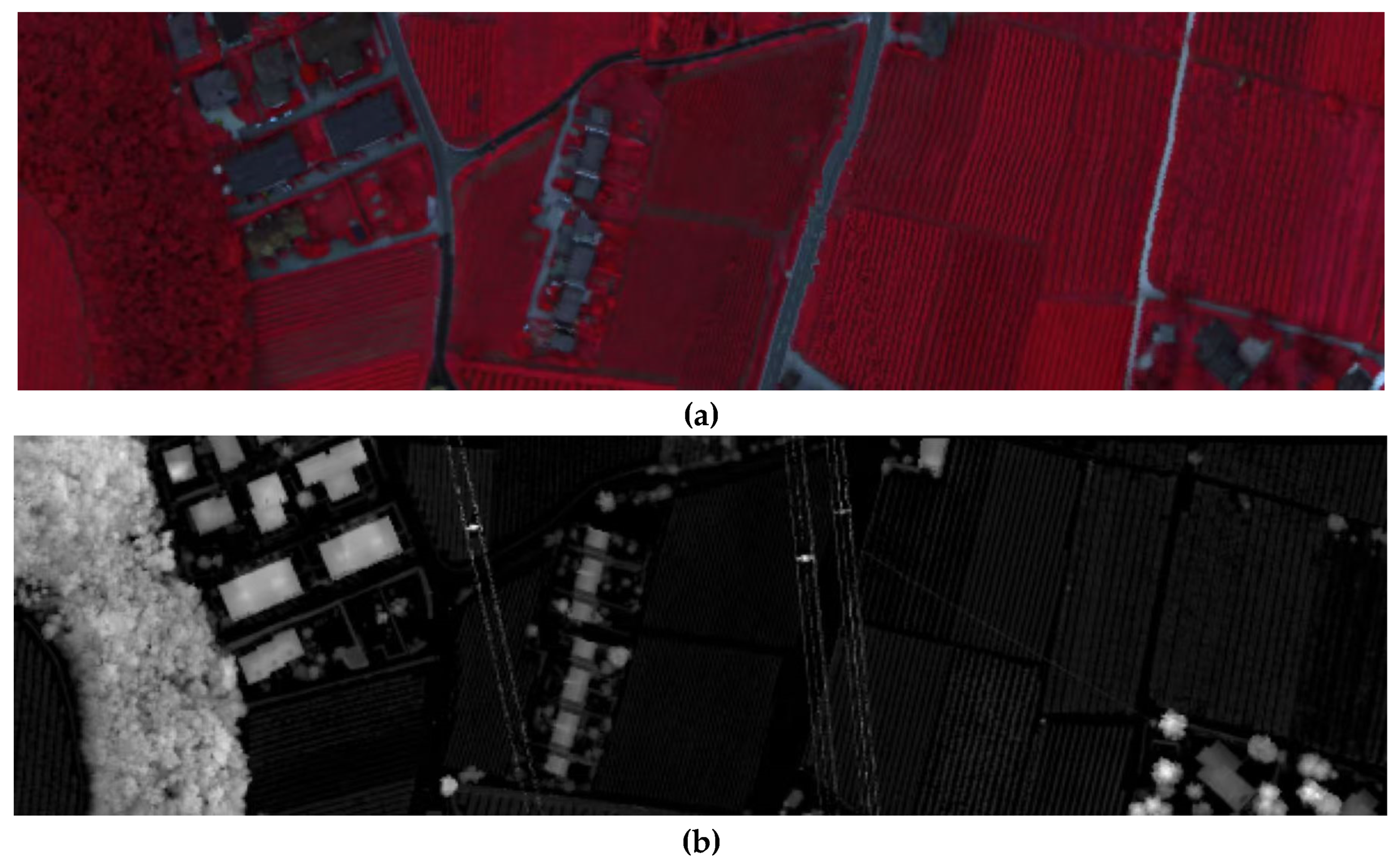
58]: The Trento dataset comes from a rural farm area south of Trento, Italy. The image measures 600 × 166 pixels with a resolution of 1 m. There are 63 spectral bands in the hyperspectral data. These bands range from 402.89 nm to 989.09 nm. The LiDAR data provides a single band of DSM information to show height. Six categories are labeled in the ground truth. These classes are apple trees, buildings, ground, woods, vineyard, and roads. The main challenge is that different plants look similar in the spectrum. Also, the layout of the farm fields is complex.
Figure 6 shows the color composite and the LiDAR map.
Table 2 details the sample counts for training and testing.
- (3)
MUUFL dataset [
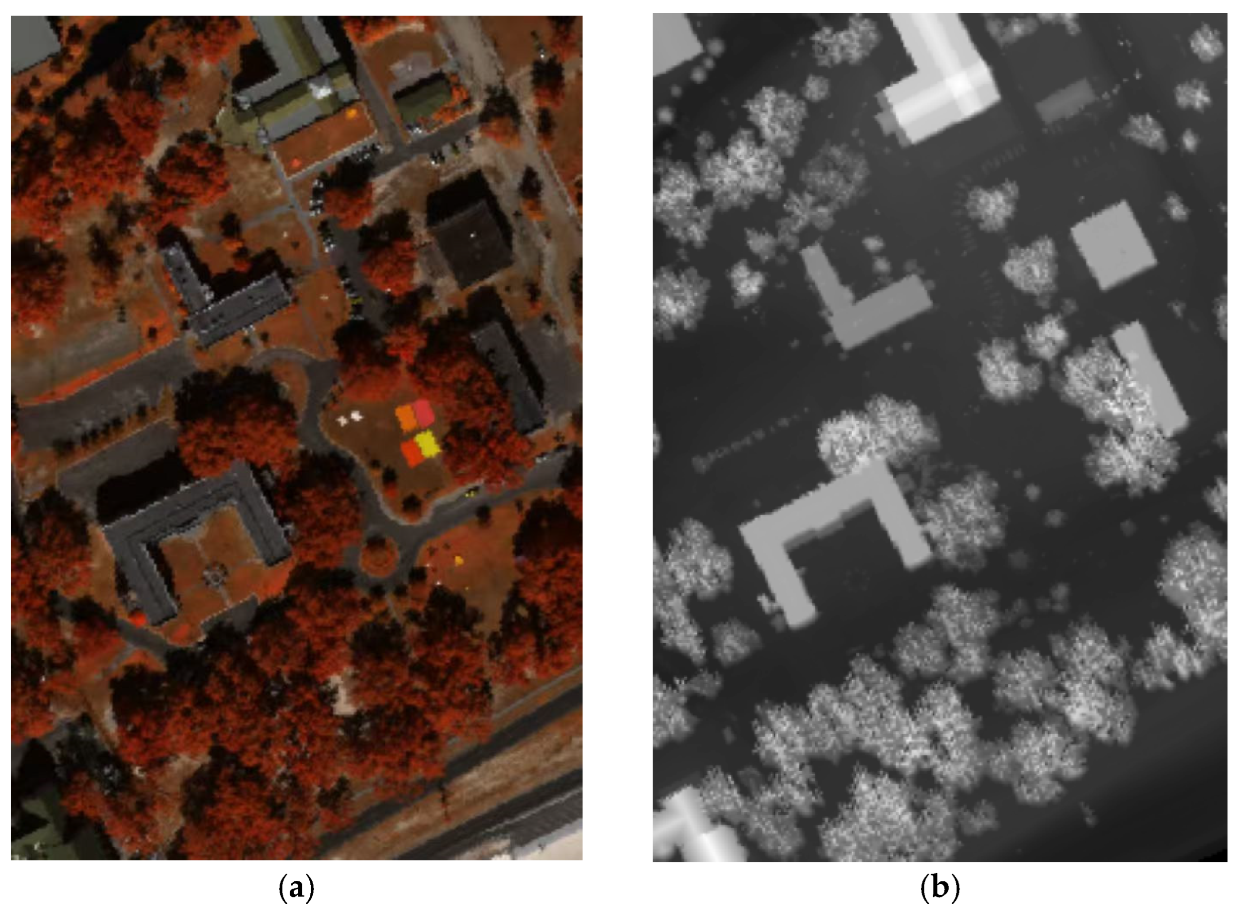
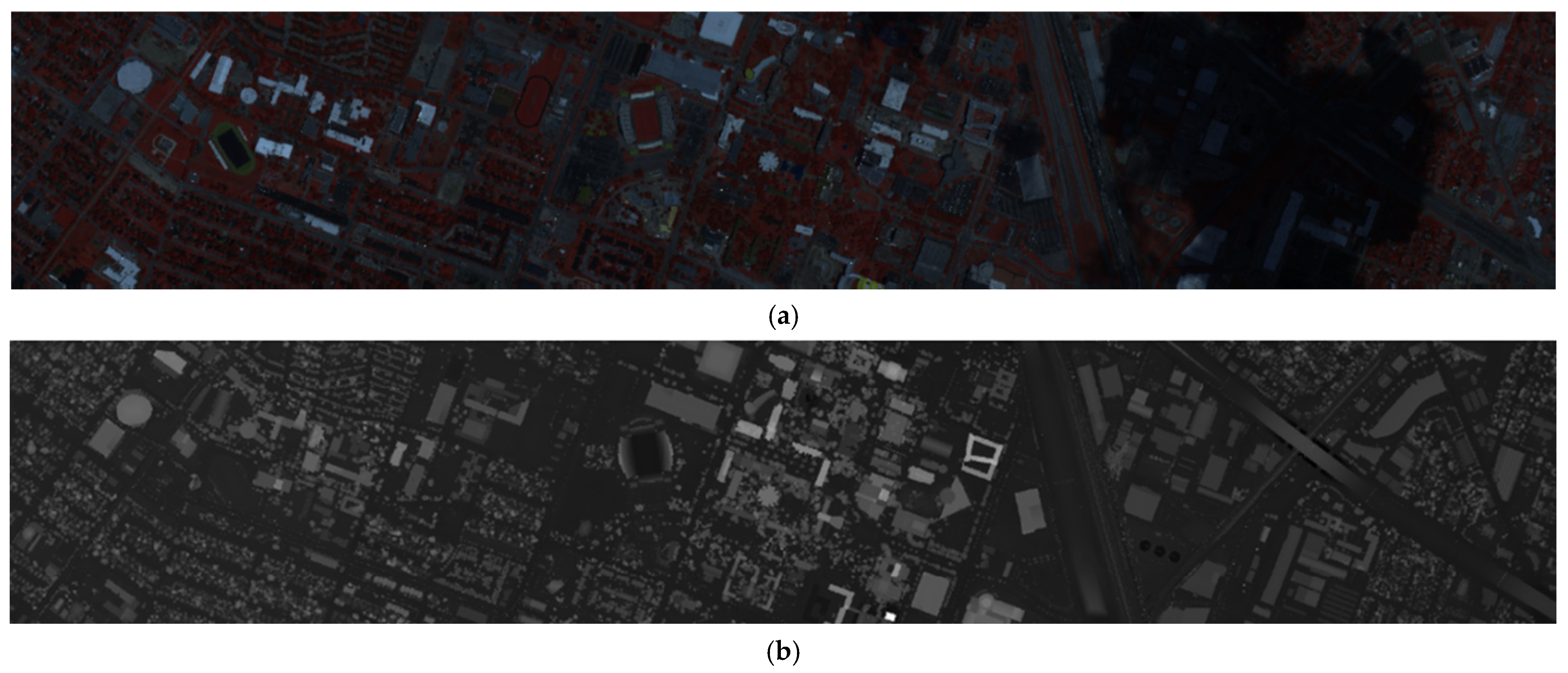
59]: The MUUFL (Multi-User Universal LiDAR and Fusion) Gulfport dataset was acquired over the University of Southern Mississippi Gulfpark Campus in Long Beach, Mississippi, USA. This dataset features a spatial dimension of 325 × 220 pixels with a 1 m spatial resolution, offering finer spatial detail compared to the Houston2013 dataset. The hyperspectral imagery contains 64 spectral bands covering the spectral range of 367.7 nm to 1043.4 nm, while the co-registered LiDAR data consists of two elevation-related channels capturing terrain characteristics. Ground reference data classify the scene into 11 thematic classes, including natural land-cover types, anthropogenic features, as well as water and building shadow categories.
Figure 7 displays the pseudo-color HSI composite and the LiDAR DSM visualization.
Table 3 lists the training and testing sample numbers for each class across the three datasets.
3.2. Classification Results and Analysis
The experiment ran on a workstation featuring an Intel i9 CPU and 64 GB RAM. Python version 3.8 served as the programming language. Model development took place in the PyCharm 2025 IDE. It was implemented using the PyTorch 2.1.2 deep learning framework. The training was carried out on the NVIDIA GeForce RTX 3080Ti GPU, with 300 training epochs, a batch size of 48, and an initial learning rate of 0.01 using the SGD optimizer.
The performance of the presented approach for HSI-LiDAR fusion classification was assessed, and six representative deep learning-based approaches were selected for comparative analysis: EndNet [
34], TB-CNN [
41], S2ENet [
60], FusAtNet [
46], ExVit [
61], and M2FNet [
62]. These methods represent different paradigms in multi-source remote sensing data fusion, ranging from attention-based architectures to convolutional frameworks and hybrid vision transformer designs. Comparison methods were chosen for strong results on HSI-LiDAR benchmarks and using diverse feature extraction and fusion strategies. Each method is described below:
EndNet: This method uses an encoder–decoder structure built for multi-source data fusion. The encoder extracts multi-scale spectral–spatial–elevation features by down sampling steps. The decoder recovers spatial details using skip connections for pixel-level classification.
TB-CNN: This approach uses a two-branch CNN structure for HSI-LiDAR data processing. Deep convolution layers extract spectral–spatial features from hyperspectral imagery and elevation patterns from LiDAR data. Features are combined at middle layers for joint representation.
S2ENet: This method uses a spectral–spatial–elevation network that combines multi-dimensional convolutions to extract spectral signatures, spatial contexts, and elevation characteristics. Channel and spatial attention improve feature representations for classification.
FusAtNet: This method employs a dual-branch design with residual modules. Hierarchical information from HSI and LiDAR sources is obtained separately. Attention modules highlight key spectral, spatial, and elevation cues. Adaptive fusion produces representations for classification.
ExVit: This approach utilizes vision transformers for HSI-LiDAR classification. Image segments are considered as individual units. The model uses self-attention to model distant relationships within spectral and elevation domains. Cross-modal attention supports data interaction between sources.
M2FNet: This method employs a multi-scale 3D–2D mixed CNN design to extract spatial–spectral features from HSI and elevation features from LiDAR data simultaneously. The extracted features are then fed into a novel encoder combining a mathematical morphology-based feature enhancement (FE) module and a dilated convolutional module (DConvformer) for efficient heterogeneous data fusion. This lightweight end-to-end architecture captures high-order multi-scale features while substantially reducing training parameters.
Three common indicators are used to measure classification results. These include overall accuracy (OA), average accuracy (AA), and the Kappa coefficient [
63]. OA is defined as the proportion of correct outputs among all test instances. AA is the average value of accuracy for each category, reflecting the recognition ability for every group without considering the number of samples. The Kappa coefficient reflects the consistency between predicted labels and reference labels and adjusts for agreement by chance. These indicators together reflect the effectiveness of the model. A higher score means better recognition. Each experiment was repeated ten times using different random seeds. The average and standard deviation were calculated and presented.
The Houston2013 dataset was used to assess the effectiveness of the different approaches.
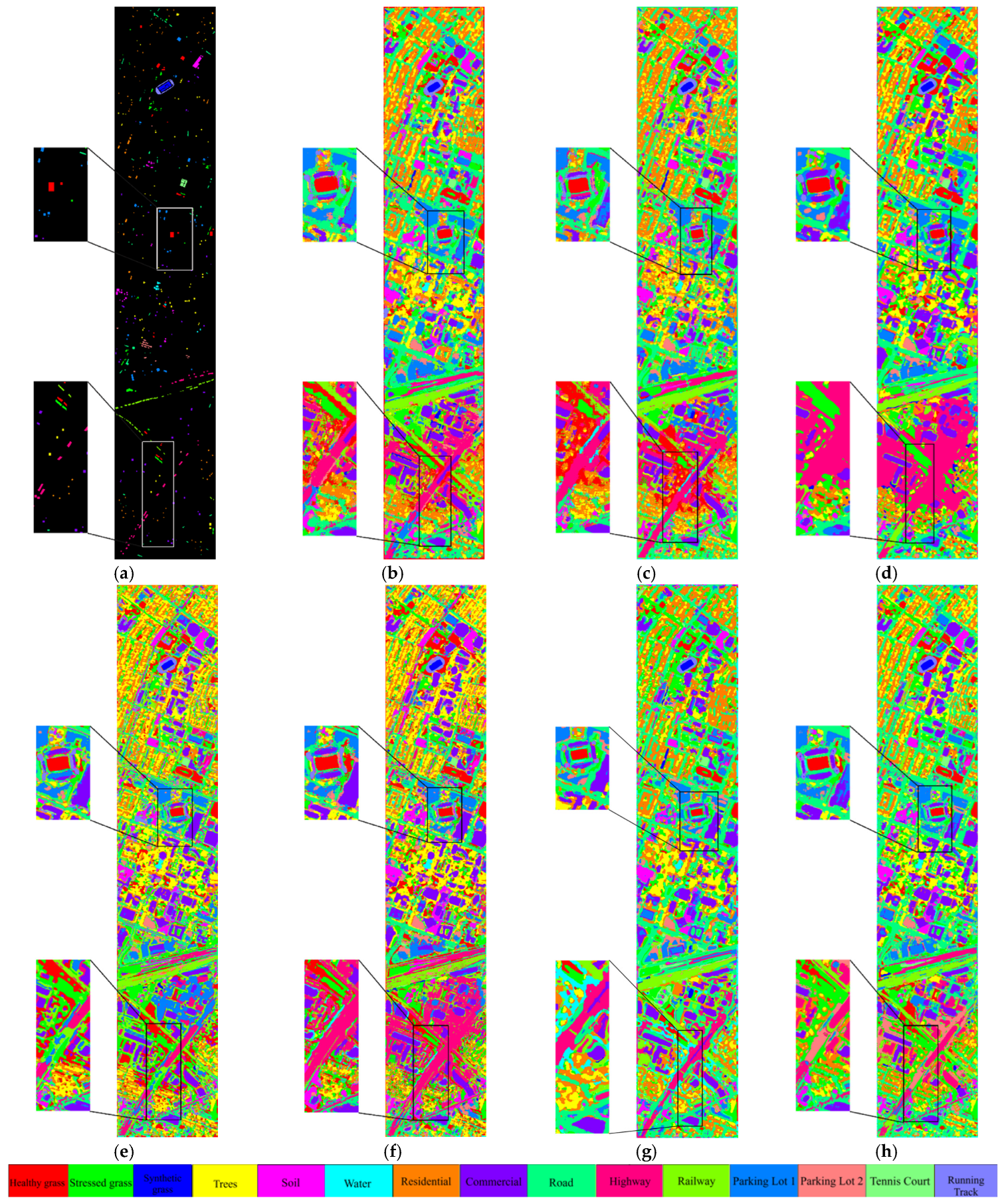
Figure 8 displays the prediction maps produced by each network and the reference map.
Table 4 lists the numerical outcomes for every class, including metrics such as total accuracy, mean accuracy, and the Kappa value. The highest scores for each class and for OA, AA, and Kappa are shown in bold font.
As shown in
Table 4, the proposed method achieves the highest overall accuracy (OA, 94.35%), average accuracy (AA, 94.66%), and Kappa coefficient (93.90%) among all the compared approaches, demonstrating superior performance in HSI-LiDAR data fusion for urban land-cover classification. The results highlight the method’s effectiveness in integrating spectral and elevation information for detailed surface identification. In terms of per-class accuracy, the proposed approach consistently outperforms or matches the best results across most categories. Notably, it achieves the highest accuracies in C2 (stressed grass, 98.38%), C3 (synthetic grass, 100.0%), and C8 (commercial, 97.81%). The outstanding performance in the commercial class can be attributed to the robust multi-level fusion of spectral and elevation features, which enhances the model’s ability to distinguish complex urban structures. Additionally, the method attains top accuracies in C5 (soil, 99.91%), C6 (water, 97.30%), and C9 (road, 95.25%), further demonstrating its adaptability across diverse land-cover types. The results indicate suitability for a range of surface classes.
Checking the classification maps in
Figure 8 confirms the numerical results. The proposed method shows smoother and more consistent spatial patterns with fewer errors and isolated mistakes. Regions containing stressed grass, soil, and water are correctly identified. The spatial continuity of urban features such as roads and commercial areas is maintained.
The model captures spectral details and spatial context effectively. It separates ground objects that look similar spectrally. Testing on the Houston dataset produced strong metric scores. Higher OA, AA, and Kappa values appear alongside better accuracy for each class. These numbers and the clear classification maps support the value of our multi-level interaction fusion strategy. Gains across many land types show that the fusion framework is stable and adapts well to different scenes.
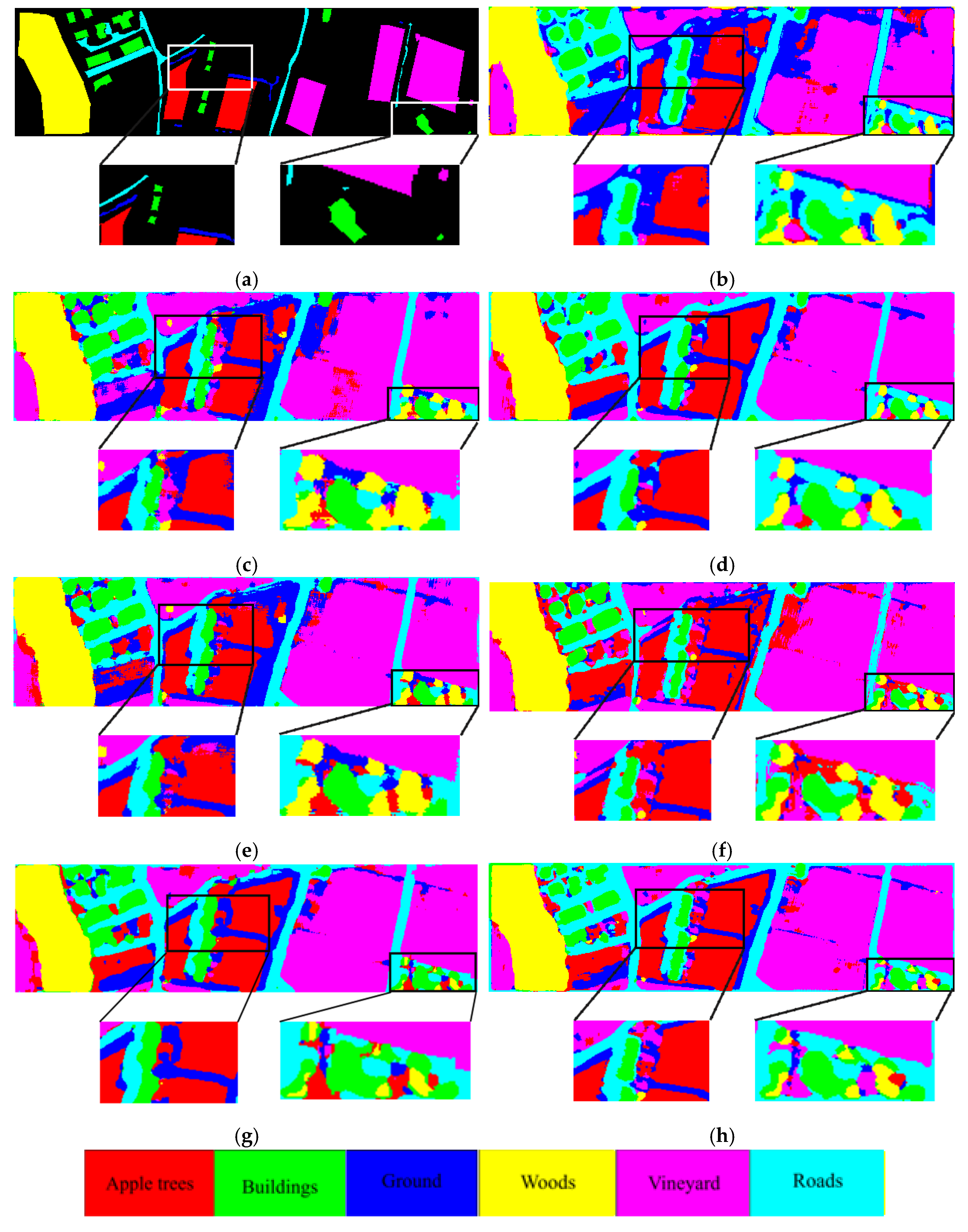
To examine the generalization ability and robustness of the proposed method, experiments were carried out on the Trento dataset and compared with five representative multimodal fusion networks, including FusAeNet, TB-CNN, EndNet, ExVit, M2FNet and S2ENet. Classification results from various approaches and the reference map appear in
Figure 9.
Table 5 lists the numerical outcomes, including the accuracy for each category, OA, AA, and Kappa value.
Table 5 shows that the proposed method performs well, with an OA of 99.78%, an AA of 99.53%, and a Kappa coefficient of 99.71%. These results exceed those for all baseline methods. The OA improvement over the best competitor (TB-CNN, OA: 99.17%) is 0.61%. The high values across all metrics show the effectiveness of the proposed cross-modal fusion strategy in extracting and combining useful features from both hyperspectral and LiDAR data. Looking at per-class accuracies, the proposed approach reaches 100% accuracy for C1 (apple trees), C4 (woods), C5 (vineyard). This beats all competing methods. For C2 (buildings) and C3 (ground), the proposed method achieves 98.9% and 99.17% accuracy. These classes are difficult because of spectral similarity and spatial complexity. The results exceed the best performance of the other methods. EndNet and ExVit show lower performance in these categories. This reveals their difficulty in separating spectrally similar classes.
This shows that the proposed approach can distinguish between spectrally similar and spatially complex land-cover types.
A closer examination of the classification maps in
Figure 9 reveals that the proposed method produces cleaner and more homogeneous classification results with fewer incorrectly labeled pixels, especially in areas characterized by complex boundaries and mixed land-cover patterns. In contrast, FusAtNet and TB-CNN exhibit more scattered misclassification in building and ground regions, while the proposed method maintains better class separation and spatial coherence. The performance difference is most evident for classes with large within-class variation or unclear boundaries, such as C2 (buildings) and C3 (ground). The higher accuracy obtained for these classes is attributed to the approach used for extracting and combining features from multiple modalities. This process makes use of diverse details available in both hyperspectral and LiDAR inputs. Single-source features become less dominant in the final representation. On the Trento dataset, this method shows strong results in terms of numbers. The produced classification maps display more distinct boundaries and structure.
Hyperspectral data and LiDAR measurements are combined using a balanced and two-way merging process. The network learns features that separate classes well. Performance remains consistent across areas with varied land-cover types.
We tested the proposed method on the MUUFL dataset. This dataset has complex land-cover types and a large imbalance in labeled samples across categories.
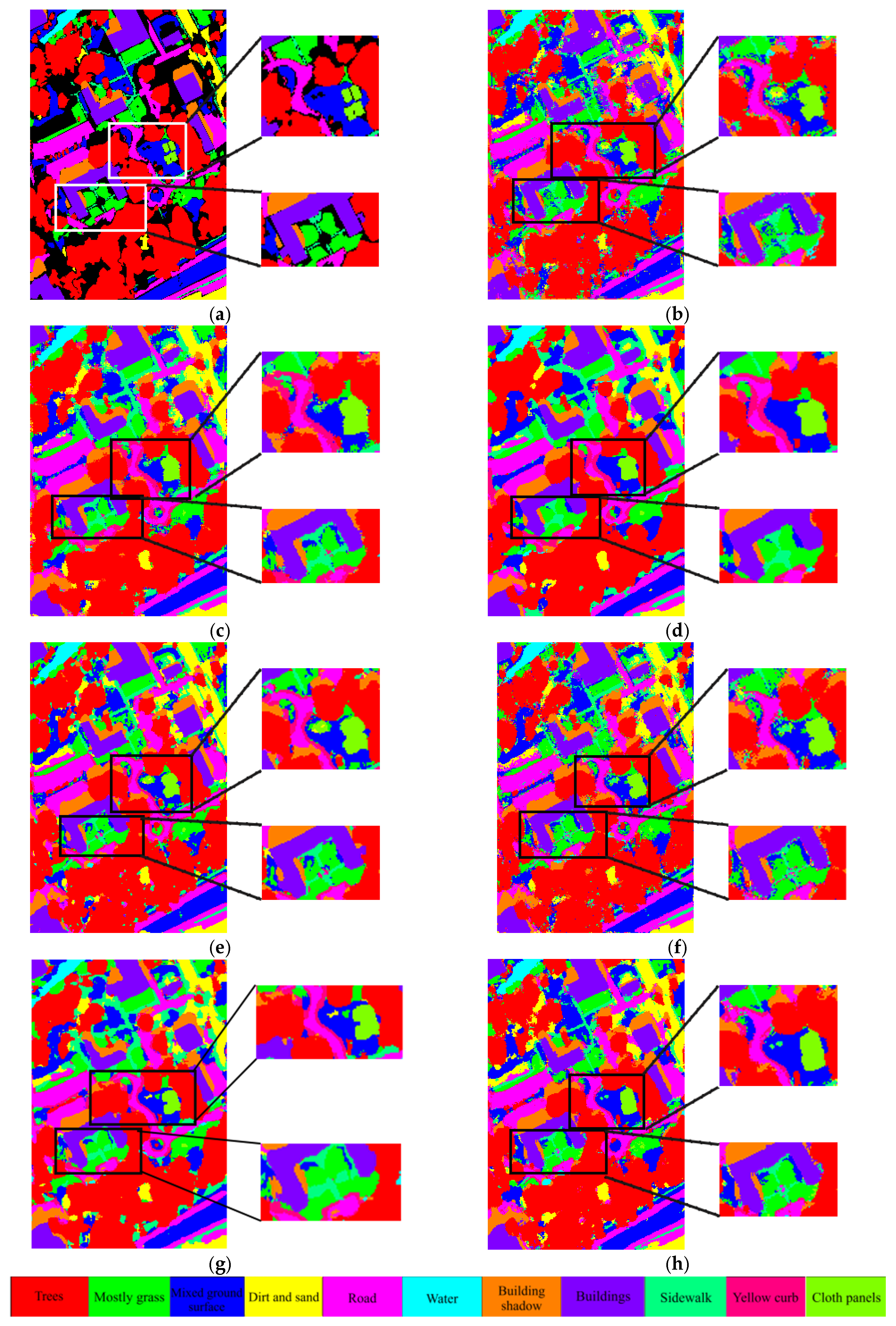
Figure 10 shows the classification maps for each method and the ground-truth map.
Table 6 lists the results, including the per-class accuracy, overall accuracy (OA), average accuracy (AA), and Kappa coefficient.
Table 6 demonstrates that the proposed method achieves an overall accuracy (OA) of 92.58%, an average accuracy (AA) of 92.95%, and a Kappa coefficient of 90.29%, surpassing all baseline methods. Compared to the best-performing competitor, ExVit (OA: 91.99%), our approach improves OA by 0.59% and Kappa by 1.54%, indicating enhanced robustness in challenging classification scenarios. In terms of per-class accuracy, the proposed method consistently achieves leading results across most categories. Specifically, it attains the highest accuracies for C1 (grass, 94.40%), C3 (tree, 88.28%), C4 (dirt and sand, 96.82%), C5 (road, 92.71%), C6 (water, 100.0%), C7 (building shadow, 98.74%), C8 (buildings, 94.82%), and C11 (cloth panels, 98.51%). These results highlight the model’s strong capability to distinguish both dominant and minor classes, even in the presence of spectral and spatial confusion.
Despite the overall strong performance, certain categories remain challenging for all methods, including the proposed one. For example, the accuracy for C9 (sidewalk, 75.95%) and C10 (yellow curb, 97.26%) is relatively lower, which can be attributed to limited labeled samples and high similarity with adjacent classes. Nevertheless, the proposed method still demonstrates improved resistance to sample imbalance and class confusion compared to other approaches.
Examination of the classification maps supports the quantitative outcomes. The developed approach yields more distinct land-cover boundaries that correspond to reference labels within areas containing intricate spatial patterns, including mixed terrain and building outlines. The dual-direction attention module in the network enhances edge delineation and limits mistakes by drawing on features derived from hyperspectral imagery and elevation measurements. Edges of trees and various terrain elements appear clearly and align with reference annotations, which demonstrates the effect of adaptive feature selection and merging. Certain difficulties persist. Scores for C7 and C10 remain low because of dispersed terrain and a lack of sufficient labeled data. Adjustments in how samples are chosen and how features are refined may help resolve these concerns. Results for the MUUFL benchmark indicate that the presented approach achieves superior performance regarding both total accuracy and accuracy for each category. The network maintains strong results for diverse environments and uneven sample counts in land-cover classification tasks within remote sensing.
4. Discussion
4.1. Model Analysis
We tested each component in the proposed network through ablation experiments on the MUUFL, Houston2013, and Trento datasets. We compared classification performance under different module settings: baseline Dynamic Group Convolution (DGC), DGC with self-attention encoding (DGC + self), DGC with bidirectional cross-attention (DGC + cross), and the complete architecture.
Table 7 presents metrics, namely, the total accuracy (OA), mean accuracy (AA), and Kappa value, for every method across all datasets. The baseline DGC framework merges hyperspectral information with LiDAR measurements, providing the input for the modified ResNet18 that applies Dynamic Group Convolution to extract features from multiple sources. Adding self-attention encoding modules (DGC + self) improves both OA and AA across all datasets. This shows that spectral and channel self-attention mechanisms improve the representation of hyperspectral and LiDAR features.
Further, introducing the bidirectional cross-attention module (DGC + cross) leads to additional improvements in performance. This module allows hyperspectral and LiDAR modalities to interact with each other in a reciprocal manner. LiDAR features are used to guide hyperspectral band selection. Hyperspectral features are employed to refine LiDAR channel fusion. The outcomes of the experiments show that this type of cross-modal interaction helps obtain additional features. This approach leads to improved accuracy in classification.
The complete model combines the outputs of the Dynamic Group Convolution backbone with those of the bidirectional cross-attention modules and achieves the highest OA, AA, and Kappa scores for all three datasets. When compared to the reference method, OA rises by 5.68%, 2.61%, and 0.97% for the MUUFL, Houston2013, and Trento datasets. These results verify the effectiveness of each component and demonstrate the necessity of integrating Dynamic Group Convolution, self-attention encoding, and bidirectional cross-attention to achieve reliable multimodal classification.
Overall, the ablation study shows that every part adds value to the overall result. The Dynamic Group Convolution backbone enables effective multimodal feature extraction. The self-attention and cross-attention units enhance how the network describes features. These units allow more detailed interaction between hyperspectral data and LiDAR data.
4.2. Impact of Patch Size on Classification Performance
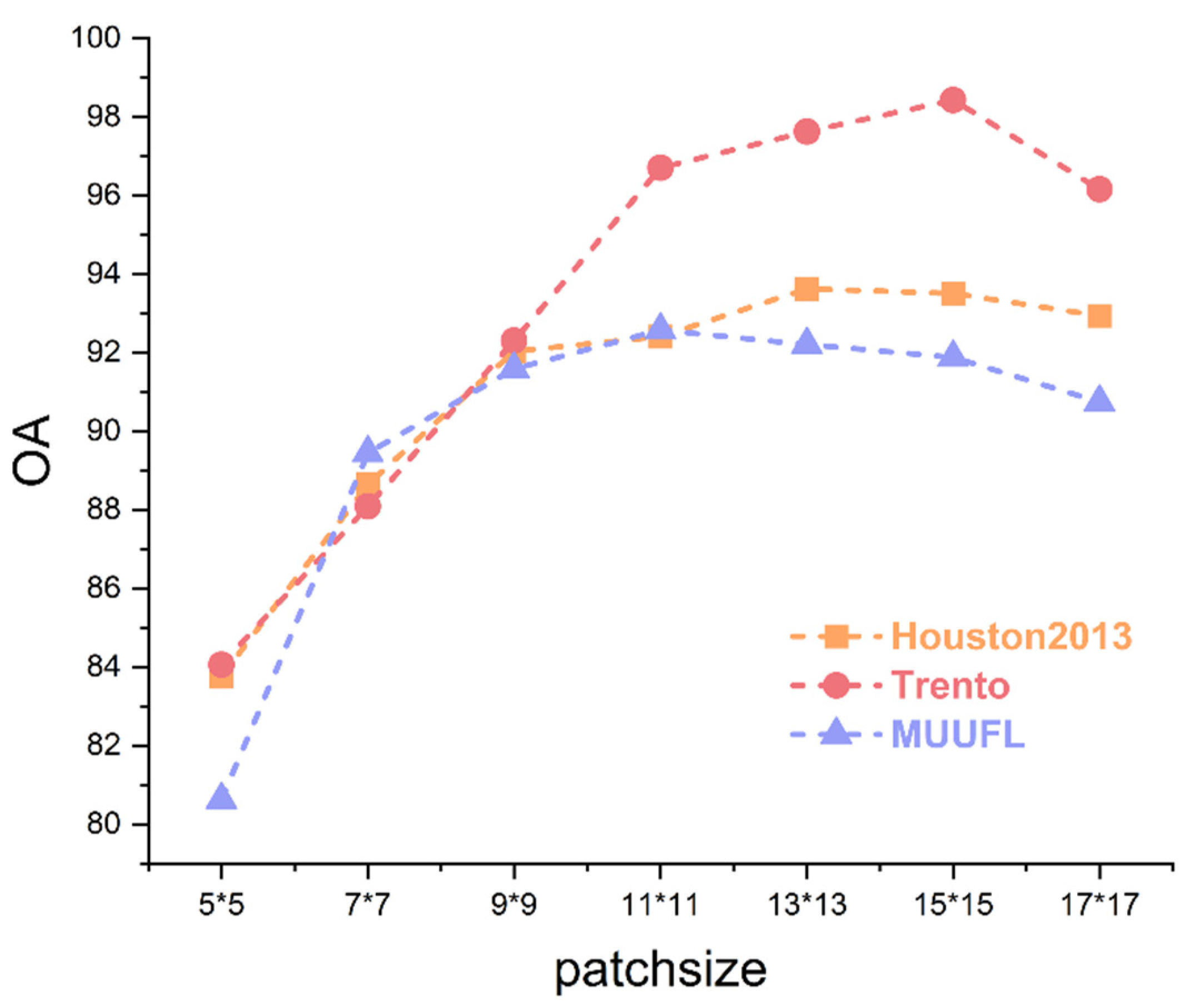
To investigate the influence of spatial context on the proposed network, we conducted a series of ablation experiments by varying the patch size of the input data cubes. The patch size determines the amount of spatial information available to the model for each sample, which is particularly critical in hyperspectral and LiDAR data fusion tasks. In this study, we evaluated the overall accuracy (OA) of our method on three benchmark datasets—Houston2013, Trento, and MUUFL—using patch sizes ranging from 5 × 5 to 17 × 17. The results are illustrated in
Figure 11.
For the Trento dataset, the OA increases as the patch size grows from 5 × 5 to 15 × 15. It peaks at 15 × 15. A larger spatial context helps separate the land-cover types in the Trento scene. Increasing the patch size to 17 × 17 causes a slight decrease in OA. Too large patches may add extra information and noise. This can hurt classification performance.
For the MUUFL dataset, the OA shows a similar trend. It rises with patch size and reaches the highest value at 11 × 11. The OA then drops. The best spatial context for this dataset is smaller. This is due to the smaller and more uniform objects in the MUUFL scene. Very large patches may weaken useful features.
For the Houston2013 dataset, the OA peaks at 13 × 13. Performance improves as patch size increases up to this value. A slight decrease happens after this point. This shows that an appropriate patch size is important for balancing enough spatial information and preventing the inclusion of extra data.
The results show similar patterns across all three datasets. The OA first increases with patch size. It peaks at a best value for each dataset. It then decreases as the patch size becomes too large. This happens because small patches fail to provide sufficient spatial context. Very large patches add unnecessary information that may slow learning. Selecting a suitable patch size is needed to improve the classification performance of the proposed network. In later experiments, patch size was set to the value that gave the highest OA for each dataset.
4.3. Impact of the Number of Selected Spectral Bands
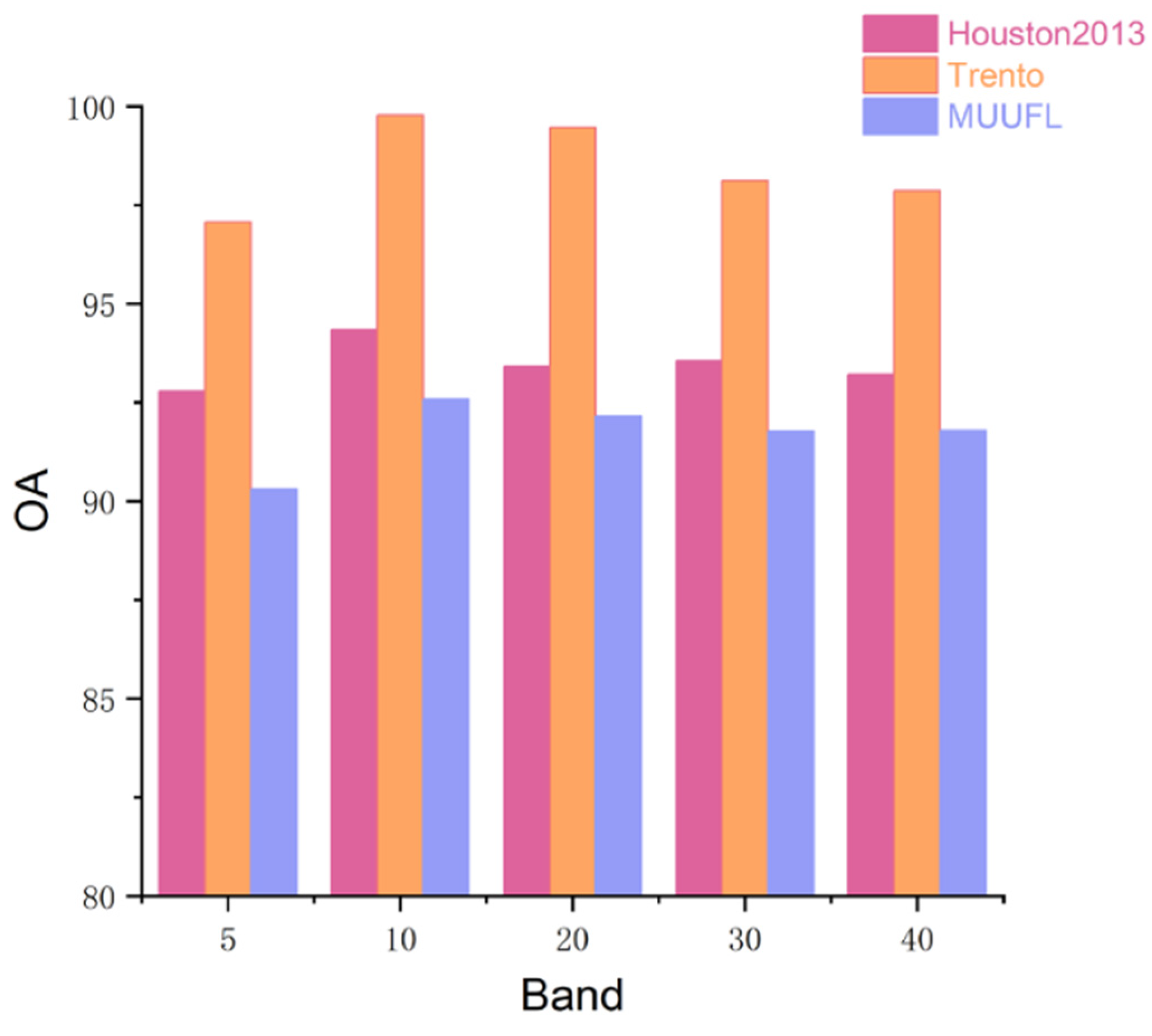
To examine how spectral band selection affects the classification performance of the proposed network, ablation experiments were carried out with different numbers of hyperspectral bands. The overall accuracy (OA) was evaluated on the Houston2013, Trento, and MUUFL datasets using 5, 10, 20, 30, and 40 selected bands, and the corresponding results are shown in
Figure 12.
Figure 12 shows that the OA values depend on the number of selected bands across all three datasets. For the Trento dataset, the OA peaks when 10 bands are selected, reaching nearly 100%. This shows that a moderate number of useful bands is enough to capture the key spectral characteristics for accurate land-cover classification. For the Houston2013 and MUUFL datasets, the OA also improves as band numbers increase from 5 to 10 but levels off or slightly drops when more bands are included. This shows that too many bands may add extra or noisy information that could reduce the model’s ability to separate classes.
These results indicate that the designed LiDAR-based band selection method is effective in identifying optimal wavelength groups for recognition tasks. Choosing an appropriate quantity of bands lowers the computational burden and enhances accuracy. Results from the ablation experiments demonstrate that the model maintains strong performance with a reduced set of bands, which highlights the effectiveness of this method.
5. Conclusions
This study introduces the DGC-BCAF network, a classification framework that exploits the joint relationship between hyperspectral spectral characteristics and LiDAR spatial–geometric information at the pixel level. The proposed architecture is developed to overcome the limitations observed in conventional fusion strategies and is built upon three key components, including an adaptive dynamic grouped convolution module, a multi-scale LiDAR feature extraction scheme, and a symmetric bidirectional cross-attention mechanism. Instead of relying on fixed convolutional structures, DGConv enables channel grouping to be learned from data, allowing the network to adjust to varying spectral–spatial distributions across different datasets. The combination of GLCM-based texture features with multi-scale convolutional representations ensures that elevation information from LiDAR data is effectively incorporated rather than being weakened during the fusion process. The symmetric bidirectional cross-attention design alleviates modality imbalance by allowing information to be exchanged in both directions, which supports mutual feature refinement between hyperspectral and LiDAR representations. As a result, informative spectral bands can be emphasized while the contribution of LiDAR channels is adaptively adjusted.
Tests on the Houston 2013, Trento, and MUUFL datasets show that the DGC-BCAF network achieves the highest scores for overall accuracy, mean accuracy, and Kappa value compared to other baseline methods. Ablation studies confirm that every component, such as dynamic grouping, self-attention encoding, and two-way interaction, is crucial for improving classification results. However, some limitations and challenges still exist. First, the two-way attention module inevitably increases the demand for computational resources. Second, our experiments revealed inherent challenges related to severe class imbalance and data scarcity. For highly similar urban materials, such as the “sidewalk” (C9) class in the MUUFL dataset, fine-grained distinction remains difficult despite efforts to balance the training sample size.
Furthermore, categories with extremely limited sample sizes emphasize the critical importance of selecting appropriate evaluation metrics. In data-scarce scenarios, metrics such as User’s Accuracy (Precision) can be disproportionately skewed by false positives from visually similar but more abundant classes, leading to an inaccurate reflection of model performance. In such cases, Producer’s Accuracy (Recall) serves as a much more robust and reliable indicator of the model’s true capability to identify minority classes.
Future research will aim to optimize the model architecture for better computational efficiency. Moreover, our primary future work will focus on developing advanced feature representation techniques to better distinguish highly similar urban materials. We will also explore semi-supervised and few-shot learning strategies to enhance model robustness in scenarios where labeled training samples are severely limited and class distributions are highly skewed. Ultimately, the DGC-BCAF framework provides a robust and effective solution for integrating multimodal remote sensing data for land-cover mapping.





 ,
,