


Highlights
What are the main findings?
- Total impact of soil type and erosion degree on the reflectivity of bare soil surface provides a polynomial ladder effect.
- The polynomial ladder effect is described in the processing of big remote sensing data in the paradigm of multitemporal soil line.
What are the implications of the main findings?
- An important step and approach is given for mapping of soil cover with high detail using big remote sensing data.
- The mechanism in formation of identical spectral characteristics of the bare soil surface of different soil types due to close values of organic matter content is shown.
Abstract
The reflectivity of the bare soil surface (BSS) is influenced by soil type, moisture, salinity, tillage, erosion, and other factors. To investigate the direct impact of erosion on the spectral characteristics of the BSS (SCBSS), a study site in the forest-steppe zone (Mtsensk district, Oryol Oblast, Russia), unaffected by salinity, carbonates, gypsum, and other factors, was selected. To suppress the influence of moisture and tillage, a multitemporal soil line (MSL) construction method was selected, which averages the influence of these factors, using the effect of big data. It was possible to reduce the influence of various factors on the SCBSS to two: zonal soil types and the extent of soil degradation from erosion (erosion degree). Soil types and erosion degree were determined by a ground survey with excavation of 488 pits/soil profiles. It was found that the relationship of soil types on the SCBSS has the form of a second-degree polynomial with a determination coefficient of R2 = 0.95. Spectral reflectance decreases across the zonal series of soils: sod-podzolic, light gray forest, gray forest, dark gray forest, podzolized chernozem, leached chernozem, typical chernozem, and meadow-chernozem soils. The influence of erosion leads to a linear increase in reflectance for each soil type in the following erosion degree series: non-eroded, slightly eroded, moderately eroded, and strongly eroded. Superimposing two functional relationships yields a distribution in the form of a polynomial ladder. This distribution maintains the general trend of a polynomial decrease in soil reflectance across the zonal series with stepwise deviations at the erosion degree. The polynomial ladder allows us to demonstrate how the erosion degree can change the spectral characteristics of one soil type to those of another.
1. Introduction
Erosion is one of the important factors determining the reflectivity of bare soil surface (BSS) [1,2,3,4], including multitemporal spectral characteristics [5,6]. The study of spectral characteristics of arable land using remote sensing data (RSD) inevitably includes an analysis of the contribution of erosion to the formation of spatial heterogeneity of the spectral characteristics of soils. Moreover, erosion is one of the most widespread processes leading to soil degradation [7,8]. The area affected by erosion is estimated at 11% of the world’s land area, with an annual loss of upper soil layers amounting to 24 billion tons [9,10]. Soil losses in the European Union alone reach 500 million tons per year [11,12]. According to the Food and Agriculture Organization (FAO) [13] estimates, the global soil loss caused by erosion may reach 40 billion tons annually. Russia is no exception, almost all arable land in different regions is subject to erosion to varying degrees [14,15,16,17]. Back in 1954, the area of land in the European part of the USSR subjected to erosion was estimated at 65 million hectares (32% of agricultural land) [18,19]. In particular, in the region of this study (Oryol Oblast), the spread of erosion processes is estimated at 800 thousand hectares. Actual and active erosion in 2016 was identified (using traditional methods during field soil surveys [20]) in the Oryol Oblast on 17.24 thousand hectares of agricultural land [21].
The complexity of ground-based methods of erosion estimation and mapping leads to attempts to model erosion processes. The volume of publications describing various approaches to modeling erosion processes amounts to hundreds of articles per year [22], and erosion models applied in different countries, for example: Bulgaria [23], Romania [24], Hungary [25], Austria and Czech Republic [26], Russia [15,27], China [28,29], etc. These are mainly works on simulation and modeling of erosion based on digital elevation models (DEM) [30,31]. The Universal Soil Loss Equation (USLE) [32] and its revised version (Revised Universal Soil Loss Equation, RUSLE) [33] are the most widely used empirical models for assessing water erosion worldwide.
Methods for mapping the distribution of eroded soils and lands using RSD are increasingly being used [1,2,3,4]. The advantage of RSD over modeling is a more accurate detection of actual erosion sites and areas. In turn, RSD processing for detecting erosion can be carried out using direct methods based on the analysis of BSS [34] and indirect methods based on vegetation indices (VIs) [35,36]. Indirect methods are subject to type II errors—indication of vegetation suppression due to reasons unrelated to erosion. Direct methods for interpreting the BSS are complicated by the lack of unified methods for identifying the BSS in RSD [37,38,39,40,41]. Attempts are still being made to identify the BSS as a threshold of the VIs, which is incorrect even theoretically [42]. In a review article on identifying the BSS [43], 191 articles were considered. One of the relevant and promising methods is the graphical identification of the BSS in the spectral neighborhood of the soil line (SNSL) paradigm [44,45] and neural network recognition of the BSS [34].
Having chosen the analysis of BSS in the paradigm of SNSL as a direction of research, it is necessary to consider the factors influencing the spectral characteristics of the BSS (SCBSS). The history of studying soil properties by reflectivity goes back more than half a century [46,47,48]. The multifactorial influence of soil properties on reflectivity is observed, including: moisture, particle size distribution, lithology, content of carbonates and salts, etc. [46,49,50,51,52,53,54,55,56,57,58,59]. Partially, the spectral images were obtained in the laboratory conditions in a form of libraries [60,61,62,63,64,65,66,67,68,69,70,71,72].
Modern studies confirm that the SCBSS are influenced by many factors: the spectral characteristics of soil type and hierarchy level (order, group, and series) [38,73,74], temperature [75], moisture [76], contents of organic carbon [40,77,78,79,80], readily soluble salts (soil salinization) [81,82], gypsum [83], and carbonates [84], texture [85], and the actual subject of this study—soil erosion [1,2,3,4].
The aim of this research is to identify the influence of soil erosion factor on the SCBSS in the zonal series of soils in the European part of Russia against the background of other factors.
2. Materials and Methods
2.1. Materials
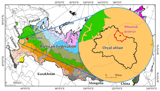
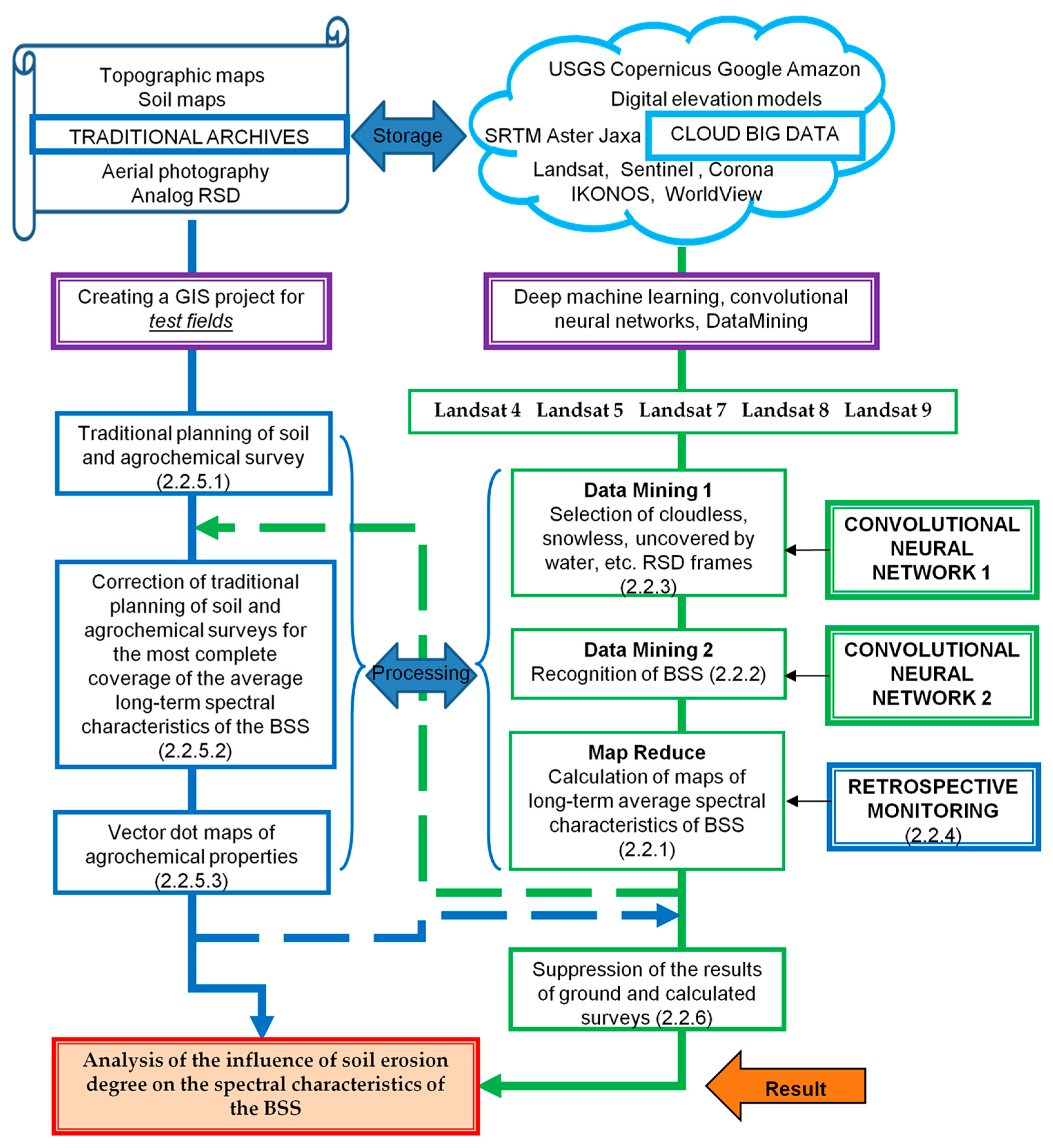
Simultaneously studying the influence of all factors on soil spectral reflectance is difficult, if at all possible. Therefore, when selecting a study site, it is necessary to narrow the scope of the study to eliminate the influence of some factors. First, the influence of land use types can be limited to just one—arable land—since erosion is primarily a consequence of anthropogenic impacts on cropland. Second, it is possible to study arable land where the content of carbonates, gypsum, and readily soluble salts is low enough to influence the SCBSS, as the area of erosion on arable land is larger than the area of readily soluble salts, gypsum, and carbonates. The Mtsensk district of the Oryol Oblast meets these conditions (Figure 1).
Figure 1.
Location of the study area (the border of the Mtsensk district is marked in red) on the map of natural zones of Russia according to natural-agricultural zoning [86].
The studied arable lands are located in north of the Oryol Oblast, in the forest-steppe zone [86,87], in the transition zone from leached and podzolized chernozems to gray forest and sod-podzolic soils [88]. The altitude above sea level within the study area is 140–170 m; the sum of active temperatures is 2150 °C; and the annual precipitation 680–700 mm. The moisture coefficient, which is defined as the ratio of the annual precipitation to the annual evaporation, is 1.1 (sufficient moisture supply); the continentality coefficient is 158. The main agricultural crops are: winter wheat, spring barley, oats, legumes, potatoes, sugar beets, hemp, and corn for green mass [89].
- (1)
- To implement the method of retrospective monitoring of soil and land (or soil–land) cover, the following spatially distributed information was used in the work: topographic maps and thematic materials at a scale of 1:25,000, high spatial resolution RSD (IKONOS, GeoEye-1, WorldView, etc.) [90], and medium spatial resolution (Landsat, Sentinel from 1984 to 2023) [91,92], as well as archival data from 1968 and 1975 (CORONA) [93].
- (2)
- When constructing a multitemporal soil line (MSL) for each pixel of RSD, the work used archives of Landsat 4, 5, 7, 8, 9 level 1 scenes/frames from 1984 to 2023. The ATCOR module is used for atmospheric correction—the ERDAS 2015 Imagine software package [94].
2.2. Methods
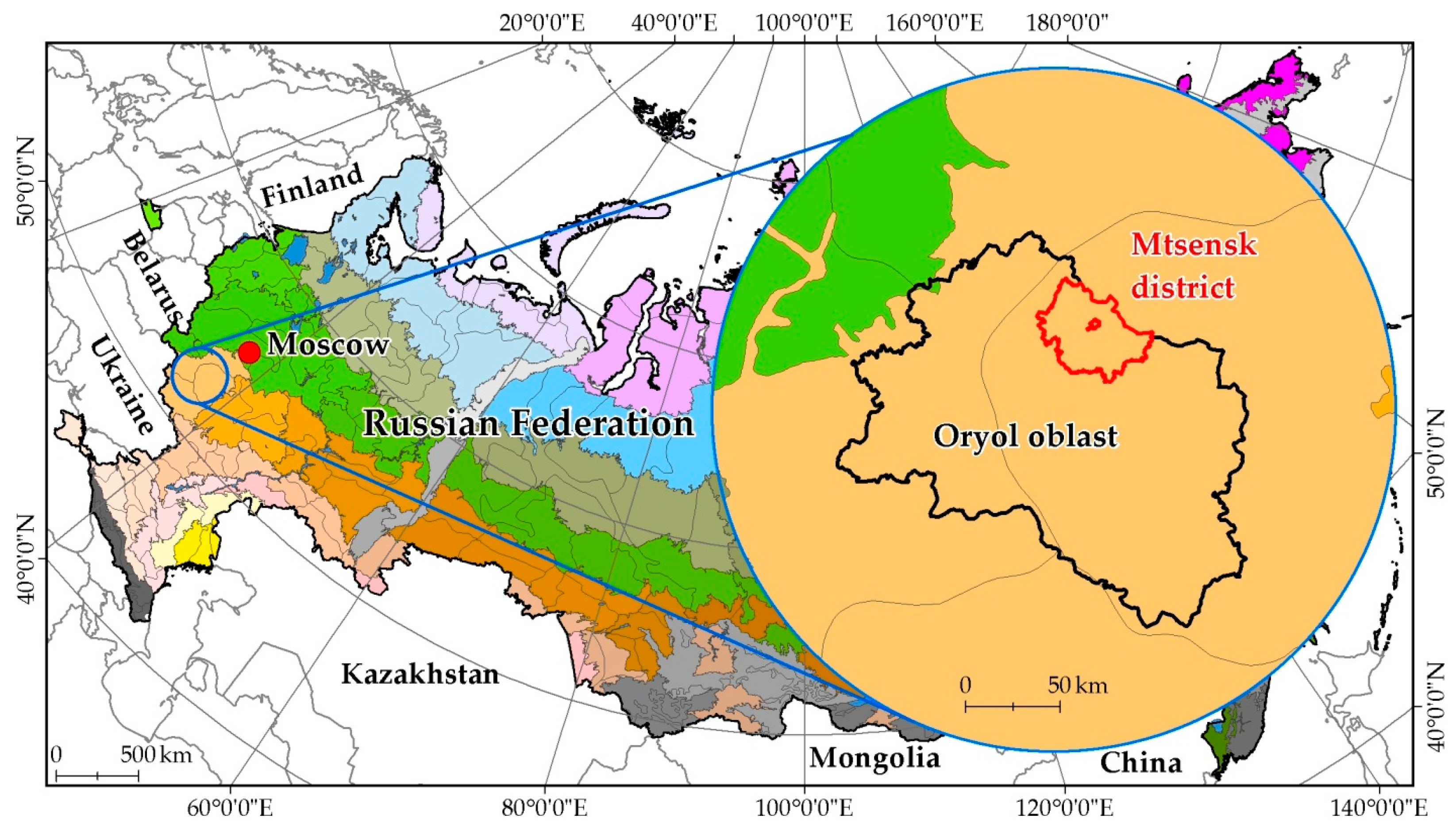
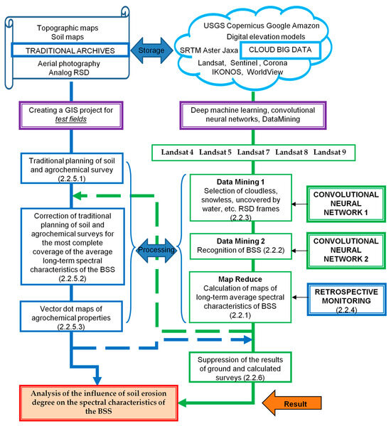
Figure 2 shows the flowchart of this study. The scheme has three main blocks: first, a block for organizing traditional field surveys based on archival materials; second, a block for calculating MSL coefficients and constructing their distribution maps; and third, a block for analyzing the obtained ground-based and spectral information. In addition to these three blocks, the research scheme shows the application points (nodes) of the BRSD processing methods, in the form of two neural networks and retrospective soil–land cover monitoring technology.
Figure 2.
Research flowchart. The number in brackets indicates the section, where the detailed description of method is given.
In two places, the blocks interact with each other. The block for constructing multitemporal spectral characteristics is used to adjust the locations of traditional field survey points. The results of ground surveys, in turn, are used in the analytical block. The flowchart also shows the hierarchical correspondence of the stages of work in blocks—storage, processing, and result.
2.2.1. Calculating of Multitemporal Soil Line (MSL) Coefficients
The main method for processing RSD in the big remote sensing data (BRSD [95]) mode in the present study is the construction of MSL in the SNSL paradigm. The SNSL paradigm means that the ellipse of possible pairs of RED and NIR values in the same spectral plane are located between the area of soot (black carbon [96,97,98]—traces of agricultural fires [42])—and straw (crop residues). From the SNSL paradigm it follows that the BSS in remote sensing scenes cannot be identified as a VI threshold [42].
The construction of the MSL assumes the possibility of constructing a “tasseled cap” [99,100] not for the RSD scene, but for each RSD pixel based on all spectral values that the pixel takes in the multitemporal series of RSD from Landsat 4, 5, 7, 8, 9 from 1984 to the present (2023) (Figure S1a). Hundreds and thousands of identical Landsat frames have been accumulated for each point on the Earth’s surface. MSL calculations fold thousands of spectral characteristics of each pixel into a compact set of MSL coefficients, i.e., extract information from the multitemporal archive in the BRSD mode.
For each pixel (or sampling unit), let , , denote the RED and NIR values for all dates classified as bare soil. The multitemporal RED–NIR distribution was approximated by a bivariate normal distribution with empirical mean vector [101]:
and empirical covariance matrix:
The center of the approximation ellipse is therefore:
Let be the eigenvalues of , and let be the eigenvector associated with . The MSL was defined as the major axis of the ellipse, i.e.,:
In slope-intercept form, this line can be written as:
The coefficient was calculated as the distance from the ellipse center to the origin of the RED–NIR spectral plane [42,102] (Figure S1b):
Here, and are the RED and NIR values for observation , is the number of bare-soil observations, is the ellipse center, and and are the slope and intercept of the MSL.
2.2.2. Allocation of BSS on RSD
To construct the MSL, it is necessary to identify the elliptical distribution area of the BSS in each RSD scene. This is impossible to accomplish in the VI threshold mode, but it is quite possible to directly identify “tasseled caps” on the graph manually [42]. Hundreds and thousands of RSD scenes that must be processed somewhat, reduce the productivity of the MSL calculations. Performance can be increased using a dataset generated by manual decoding of the BSS. Machine learning can be performed using this dataset to automate RSD filtering. This problem was solved through the development and application of a neural network [34].
The method involves training a neural network based on a dataset. The dataset is a series of Landsat scenes from 1984 to 2020, in which the BSS is identified. The theory of the SNSL was used to identify the BSS areas. According to this theory, the BSS occupies a specific location on the “tassel cap”. The location of the SNSL only partially coincides with the soil line for NDVI [103]. The trained neural network can identify BSS in any Landsat image under similar soil and climatic conditions.
In this study, deep machine learning was used. We applied the popular neural architecture for image segmentation U-Net [104], the Rectified Linear Unit (ReLU) activation function and batch normalization [105], the Dice Loss function [106], and the Adam optimization algorithm [107].
The development and application of a neural network for recognizing BSS are described in detail in a paper of 2022 [34]. No additional neural network training was performed for this study. The training described in [34] was used. To evaluate the performance of the previously trained neural network in the current study area, a small acceptance sample was created. This sample was formed from 10% of the Landsat scenes used in the study. As in the 2022 study [34], the BSS was manually detected on these scenes. The overall Intersection over Union (IoU) metric of the proposed model on the current validation set is 0.79.
2.2.3. Screening of RSD Archives
Most RSD scenes do not contain BSS, due to their cloudiness, snowiness, image acquisition artifacts, etc. Recognizing BSS in such scenes creates unnecessary load on computing power. A more optimal approach is to pre-filter of the RSD for BSS detection. Less labor-intensive machine learning methods can be used to solve this problem.
A good machine learning method for filtering the suitability of RSD is gradient boosting [108]. A detailed description of the method implementation is given in the 2021 paper [35]. A manually created dataset was used, which contains an array of RSD fragments indicating vegetation, cloudiness, waterlogging, snow, etc. The CatBoost 1.2.8 [109] library of the Python programming language 3.13 [110] was used.
The datasets for training the neural network and for gradient boosting are identical. The tasks are also the same—binary image classification (“suitable” or “unsuitable”)—was performed. The standard convolutional neural network architecture for binary classification was used. Such architectures typically [111,112] consist of a pair of convolutional blocks followed by a pooling layer and a pair of fully connected layers. A convolutional block, in turn, contains a convolutional layer, a normalization layer, an activation layer, and a max pooling layer. The shape of the input layer is 128 × 128 × 8. Here, the 8 bands include: RED, GREEN, BLUE, NIR, SWIR1, SWIR2, NDVI, and binary field mask.
2.2.4. Retrospective Monitoring of Soil and Land Cover
The construction of the MSL in the paradigm of the SNSL was developed for arable lands. Outside arable lands, the BSS may be associated with roads, quarries, buildings and other anthropogenic impacts of non-agricultural nature. Erosion in the present study is also a factor of the arable land degradation. The arable land and sown areas in Russia during the study period varied significantly from 134 to 77 million hectares [113,114]. It is possible to obtain the boundaries of arable land for this period (1984–2023) with the accuracy of the present study (cartographic scale of 1:10,000 and more accurate) using retrospective monitoring technology [115]. This method allows reconstructing changes in the arable land boundaries in the period from 1968 to the present day. In this research, it was used to define the boundaries of fields that ceased to be cultivated (were abandoned) during the study period. Special detailing is carried out from 1984 to the present day, when high dynamics of arable land area in Russia was observed [113]. The method accuracy corresponds to the traditional mapping scale of 1:10,000 [116,117], and it requires a GIS project of a certain composition and quality (georeference and atmospheric correction). The methodology is described in a series of works from the period 2014–2020 [116,117,118,119,120,121,122].
2.2.5. Field Soil and Agrochemical Surveys
The results of the work depend on the field survey. We have previously examined this issue in several papers [123,124]. The selected option was to lay out soil pits according to the field survey guidelines adopted in Russia, with adjustments for the SCBSS.
- (1)
- Verification of the SCBSS and maps based on them requires ground-based examination. To do this, it is necessary to determine the locations of soil pits and collect samples for agrochemical analysis. For this purpose, according to instructions [21,125], topographic maps, relief, and RSD are taken into account. Modern approaches for these purposes utilize GIS projects. The composition of georeferenced GIS layers: topographic maps, if possible aerial photography or unmanned aerial vehicle (UAV) data, a DEM [30,31], and current high- and medium-resolution RSD.
- (2)
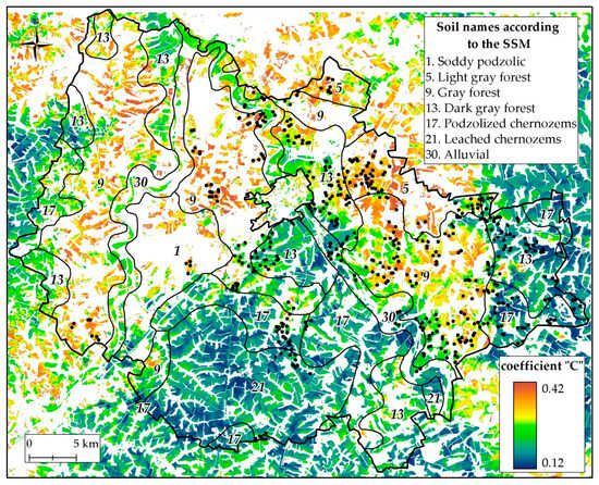
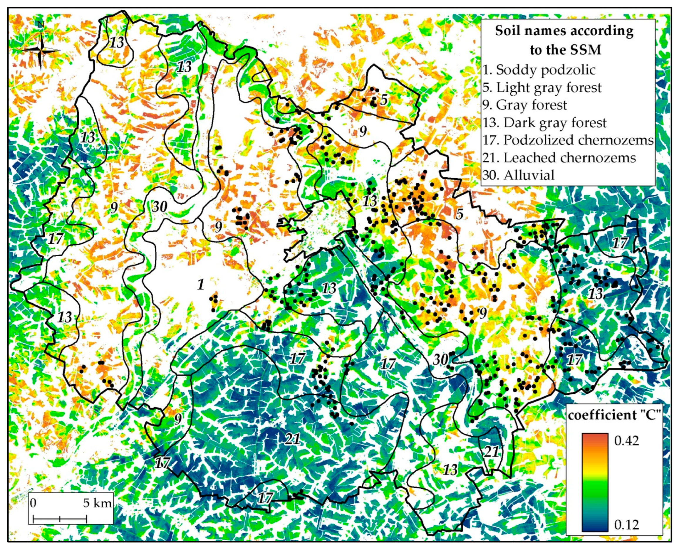
- Traditional field survey guidelines [126] do not allow for the identification of soil cover structure (SCS) [127,128,129] over large areas. The detail of the present study corresponds to a resolution of 30 m [123], which precisely requires a level of research corresponding to SCS mapping. Therefore, the soil pits/profiles were laid out taking into account the map of coefficient “C” of the MSL (Figure 3). The pits were laid out on 160 agricultural fields in the number of 488 (Figure 3). The entire range of values of the coefficient “C” of the MSL was taken into account for all fields.Figure 3. The “C” coefficient map of the MSL, soil type contours of the state soil map (SSM) and sampling points/pits location.
- (3)
- The pits were excavated to depths ranging from 65 to 160 cm. This depth was intended to reveal the total thickness of humus (also known as humus-accumulative or organomineral) horizons and allow for a description of the erosion degree. For each pit, a soil description, photography, and sampling were conducted. The GPS receiver (Garmin, Olathe, KS, USA) was used for recording of pit coordinates. Samples were taken from each horizon within each pit to measure the organic matter (OM) content. The thickness of the organogenic layer was determined with a tape.
The thickness of the humus horizon is the sum of length by depth of the A and AB layers in soil profile [130,131]. The content of OM (humus) in soil samples was determined using the Tyurin method [132], an analog of which is the Walkley–Black method [133].
2.2.6. Cartographic GIS Analysis
Cartographic analysis was conducted for calculation of regression formulas between spectral characteristics and the results of georeferenced ground-based measurements; for this the ArcGIS 10.5 [134] was used. Pairwise intersection of GIS layers created during the study was performed. The intersection results were entered into spreadsheets, allowing for graphical and regression analysis.
3. Results
3.1. Primary Results
3.1.1. GIS for Planning Field Surveys of Arable Land
To determine the locations of the soil pits, a classical GIS was formed with the following composition: topographic maps at a scale of 1:25,000, RSD of high resolution (about 1 m), archival soil and land management materials at a scale of 1:10,000–25,000, DEM with a spatial resolution of 30 m, RSD of medium resolution (30 m) for the period 1984–2023, cadastral materials. The GIS was supplemented with the boundaries of arable land at a scale of 1:5000 based on the results of retrospective monitoring of the soil–land cover (method details is shown in Section 2.2.4) and the state soil map (SSM) at a scale of 1:1,000,000 [87,135,136] (Figure 3). The area of arable land in the region amounted to 93 thousand hectares. The locations of the soil pits (method described in Section 2.2.5 is applied) are shown in Figure 3. The location of sampling points was also depended by the decision of the landowners to allow field work to be carried out on certain arable land.
3.1.2. The Map of Multitemporal SCBSS—The Map of the Coefficient “C” of the MSL
In 2023, 524 scenes from April to November were found in the Landsat archives for the Mtsensk district of the Oryol Oblast. Using a neural network (method details are shown in Section 2.2.3), 68 scenes from Landsat 4, 5, 7, 8 and 9 were selected for calculations. In these scenes, the neural network (the method procedure is shown in Section 2.2.2) recognized the distribution areas of the BSS. A total of 877,997 BSS pixels were recognized for the arable land of the Mtsensk district in 68 scenes over 39 years. For each pixel, the MSL coefficient “C” was calculated—the distance from the center of the approximation ellipse of the multitemporal BSS values of the pixel to the origin of the RED–NIR multitemporal spectral plane. The calculation was performed using at least 6 BSS values per pixel. The maximum BSS value per pixel was 58 times. All calculated values of the MSL coefficient “C” (the method procedure is shown in Section 2.2.1) are presented in Figure 3.
3.1.3. Soil Cover
During the field investigations, 488 soil profiles were laid and 7 zonal soils were detected according to the teachings of V.V. Dokuchaev [137]: sod-podzolic, light gray forest, gray forest, dark gray forest, podzolized chernozem, leached chernozem, and typical chernozem. In addition, intrazonal waterlogged (meadow) soils were identified. The location of pits for 8 soil types is shown in Figure 3. Each of these soils (except for waterlogged ones), according to the classical soil mapping and classification, have four degrees of soil degradation from water erosion: non-eroded, slightly eroded, moderately eroded, and strongly eroded soils. Consequently, 29 soil subtypes/principal qualifiers were found and described in the study area during field survey; Table 1 lists all names of 29 soil subtypes.
Table 1.
Soil cover of the Mtsensk district according to the state soil map and field survey.
Due to the incompleteness of the field soil survey (the observation was carried out only where permission from landowners was obtained), degraded variants of sod-podzolic soils and typical chernozems were not detected.
In the SSM [136], typical chernozem is absent from the 7 zonal soils, but intrazonal alluvial soils are present. No arable land on alluvial soils was found during the field survey, and calculations for this soil type were not conducted. For consistency in the numbers of the legends in Figure 3 and the analytical graphs, the correspondence of the soil names for this study and their numbering are presented in Table 1. For further analysis, it is of fundamental importance to preserve the numbering of not only those soils found during the field survey, but also of the entire range of soils in the study region.
3.2. Analytical Results
3.2.1. The Influence of Zonal Soil Types on Multitemporal Spectral Characteristics—SSM Analysis
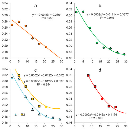
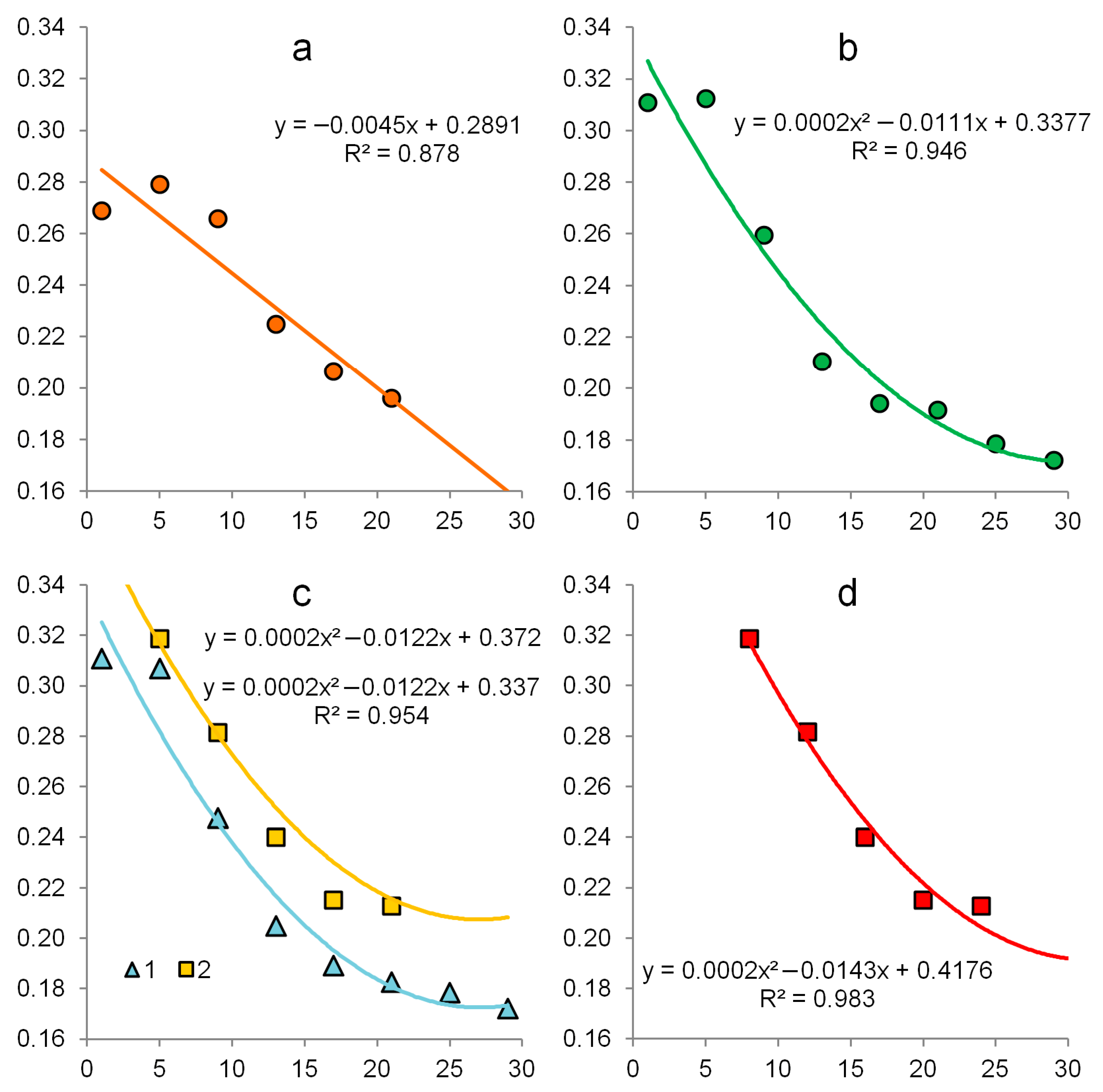
At the SSM scale of 1:1,000,000, erosion was not described in the legend. The intersection of the vector version of the SSM [88] and the coefficient “C” map of the MSL allows to calculate the average spectral values of the BSS for each position of the SSM legend. Figure 4a shows a graph of the dependence of spectral characteristics on soil types according to the SSM. The spectral brightness on the graph smoothly decreases according to a linear dependence in the next zonal row: from sod-podzolic soils to chernozems. The high determination coefficient (R2 = 0.88) indicates a practically functional relationship—the soil type determines its spectral characteristics.
Figure 4.
Graphs of the dependence of spectral characteristics on soil types. The x–axis shows the soil numbers (Table 1), and the y–axis shows the coefficient “C” values of the MSL. (a)—average SCBSS for each position of the SSM legend; (b)—average SCBSS for 9 soil types from the field survey; (c)—average SCBSS: 1—for non-eroded soils from the field survey, 2—a similar graph for strongly eroded soils; (d)—average SCBSS for strongly eroded soils from the field survey.
3.2.2. The Influence of Zonal Soil Types on Multitemporal Spectral Characteristics—Analysis of Field Data
Since the soil erosion degree is not indicated in the SSM, to compare the SSM and field survey data, the spectral characteristics of 488 ground-based sampling points were grouped into 9 zonal soil types (non-eroded and eroded soil type variants were averaged) and presented in a graph (Figure 4b). The graph in Figure 4b differs from that in Figure 4a because it has a polynomial approximation and a higher determination coefficient (R2 = 0.94). Both graphs confirm the practically functional relationship between the SCBSS and soil types.
3.2.3. The Influence of Zonal Non-Eroded Soil Types on Multitemporal Spectral Characteristics—Analysis of Field Data
Of the 488 soil pits, 288 showed no signs of water erosion. Figure 4c shows graph #1 of the effect of exclusively non-eroded soils on the SCBSS. Graph #1 is similar in shape to Figure 4b, and the dependence has an even higher coefficient of determination (R2 = 0.95). The graphs in Figure 4a–c clearly demonstrate the influence of zonal soil types on multitemporal spectral characteristics.
3.2.4. The Influence of Zonal Strongly Eroded Soil Types on Multitemporal Spectral Characteristics—Analysis of Field Data
Strong erosion was observed in 73 of 488 soil profiles, and only 5 soil types out of 8 possible. The spectral characteristics of strongly eroded soils are shown in Figure 4d. It should be noted that the dependence in Figure 4d is similar to those in Figure 4b,c. The main difference is the higher soil reflectivity values. To better demonstrate the degree of shift in the spectral characteristics of eroded soils relative to non-eroded soils, Figure 4c shows graph #2, similar to that in Figure 4d. For clarity, eroded soils are placed above their non-eroded counterparts, and the polynomial function is given with the dependence coefficients of graph #1, except for the shift along the ordinate axis. From graphs #1 and #2 it is clearly evident that erosion processes increase the reflectivity of the soil by 0.035 units of the coefficient “C” of the MSL.
3.2.5. General View of the Dependence of Multitemporal SCBSS and Erosion Degree of the Soil Cover
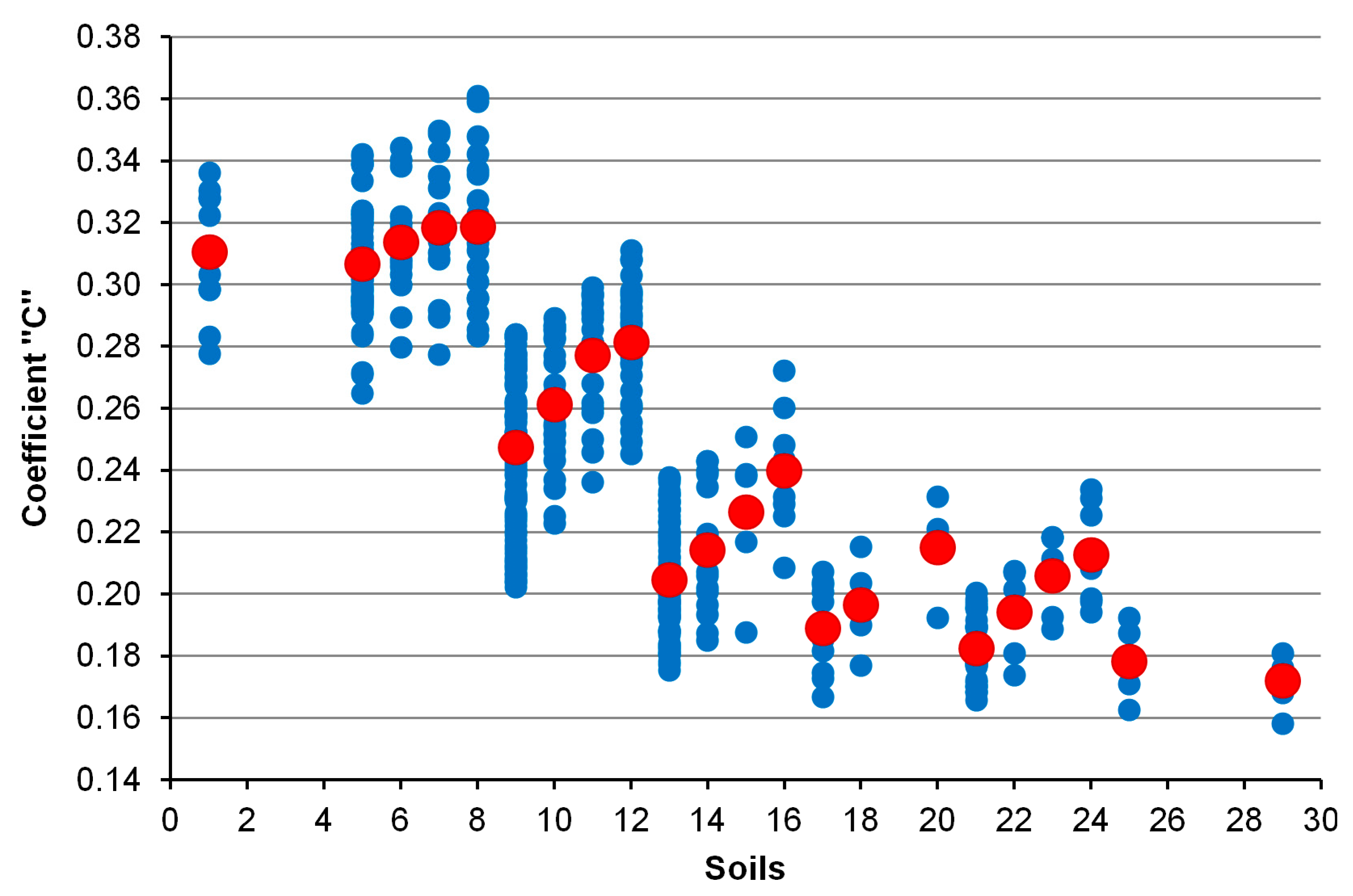
Table 1 lists the names of 29 soil types that may be encountered in the study area. Non-eroded analogs were found for 2 zonal soil types (sod-podzolic soils and typical chernozems) during the field survey. In total, spectral characteristics could be measured for 26 soil types and their eroded variants (Figure 5). Figure 5 shows all 488 ground survey points, indicating the MSL “C” coefficient values. Additionally, Figure 5 shows the average spectral values for the 26 soil types. Also Figure 5 demonstrates that the average values for each soil group by erosion degree (non-eroded, slightly eroded, moderately eroded, and strongly eroded) form polynomial relationships of soil type influence on the spectral reflectance of the BSS. For each zonal soil, the erosion degree increases reflectance.
Figure 5.
Spectral characteristics of soil types (Table 1) at survey points. The blue dots—observed values, red—average.
3.3. Analysis of the Erosion Influence on Multitemporal SCBSS
For all zonal soils for which eroded analogs were detected during field surveys, a consistent trend in spectral characteristics with varying erosion degrees is observed (Figure 4c). This trend indicates that for each zonal soil, more eroded analogues have higher reflectivity than less eroded ones. Furthermore, the main trend (Figure 4c,d) shows that, with the same erosion degree, soils maintain a decreasing trend in spectral reflectivity in the following zonal series: sod-podzolic soils, gray forest soils, and chernozems.
As a result of the superposition of these two trends, the dependence of spectral reflectance on soil types and erosion severity takes on the characteristic shape of a polynomial ladder (Figure 5). In the polynomial ladder, each erosion degree brings the spectral reflectance BSS characteristics of one soil type closer to the preceding type in the zonal series of the following list: sod-podzolic, light gray forest, gray forest, dark gray forest, podzolized chernozems, leached chernozems, typical chernozems, and meadow-chernozem.
However, the convergence of spectral characteristics during erosion varies for different soils. In gray forest soils, even severe erosion cannot change the spectral characteristics of one soil type to those of another. That is, a strongly eroded dark gray soil remains spectrally darker than a gray forest soil. The situation is different for chernozems. Strongly eroded chernozems may not differ spectrally from each other or from dark gray forest soils.
Thus, the polynomial ladder of SCBSS shows that both zonal soils and eroded analogs will fall into the same spectral range, but they will not fall randomly, but according to a functional dependence—a polynomial ladder. Thus, the influence of soil erosion on the SCBSS of zonal soils has the form of a polynomial ladder.
4. Discussion
4.1. The Physical Meaning of the Observed Phenomenon
The physical meaning of the coefficient “C” of the MSL is quite simple and is described in a series of articles [34,42,44,138]. At any given time, the arable soil can take the form of a BSS, and be covered with vegetation, plant residues, soot, water, snow, etc. [42]. The SNSL paradigm allows identifying only the BSS in remote sensing scenes [44]. A neural network allows automating this process [34]. Thus, for each pixel of RSD for 39 years (1984–2023), dozens of the BSS values can be obtained from the Landsat archives.
However, the BSS may have different moisture contents and extents of agricultural impact at different moments in time. Both parameters will influence the spectral reflectance. However, over several decades, all BSS values form an ellipse of all possible BSS values for each pixel in the RED–NIR spectral plane. This is the effect of big data: each individual value carries no information, but the set of all values of the BRSD forms a unique pixel ellipse (Figure S1b). Our study used the coordinates of the ellipse center of multitemporal spectral BSS values, which create a spectral portrait of the zonal soil (Figure 4c).
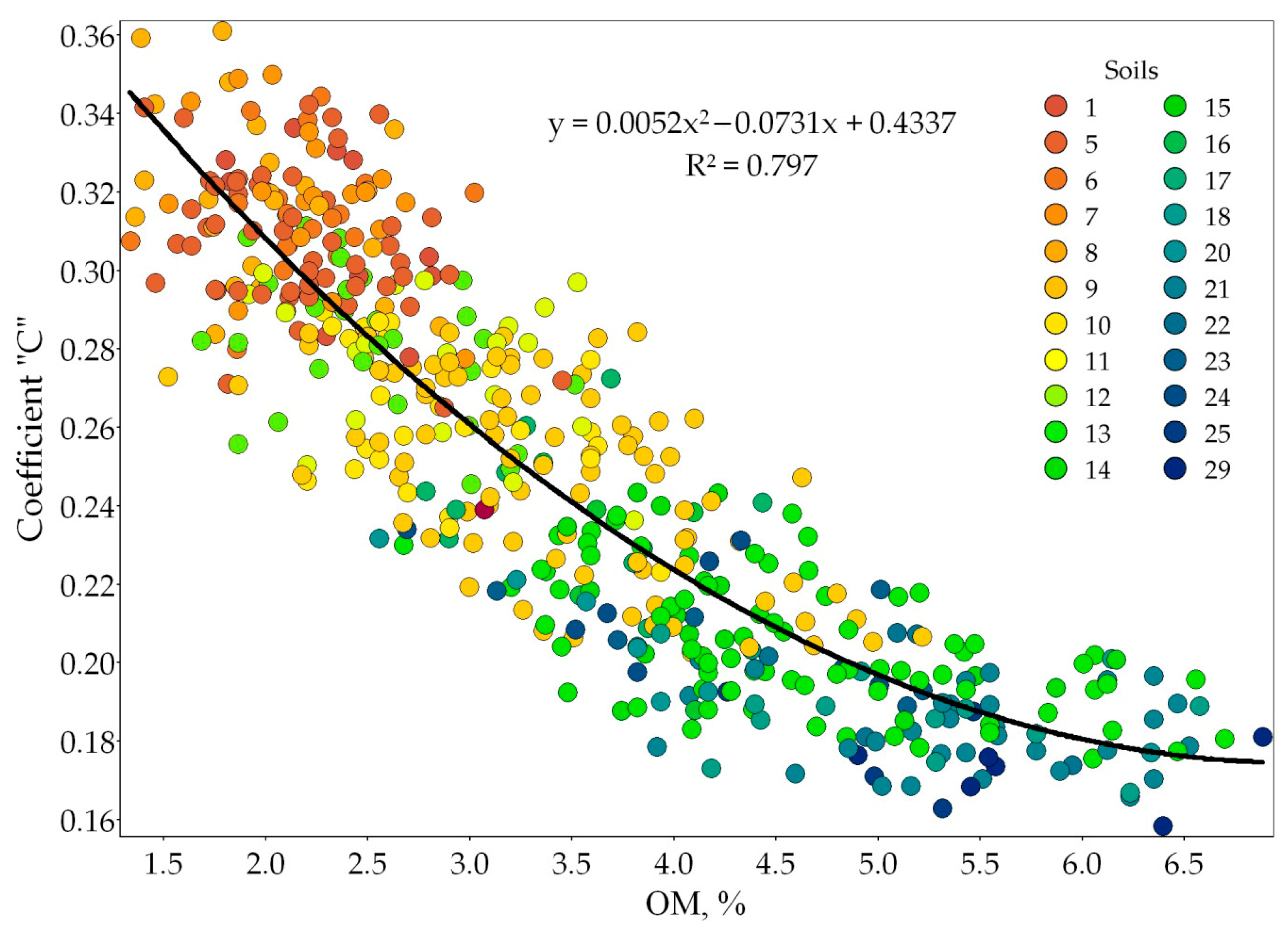
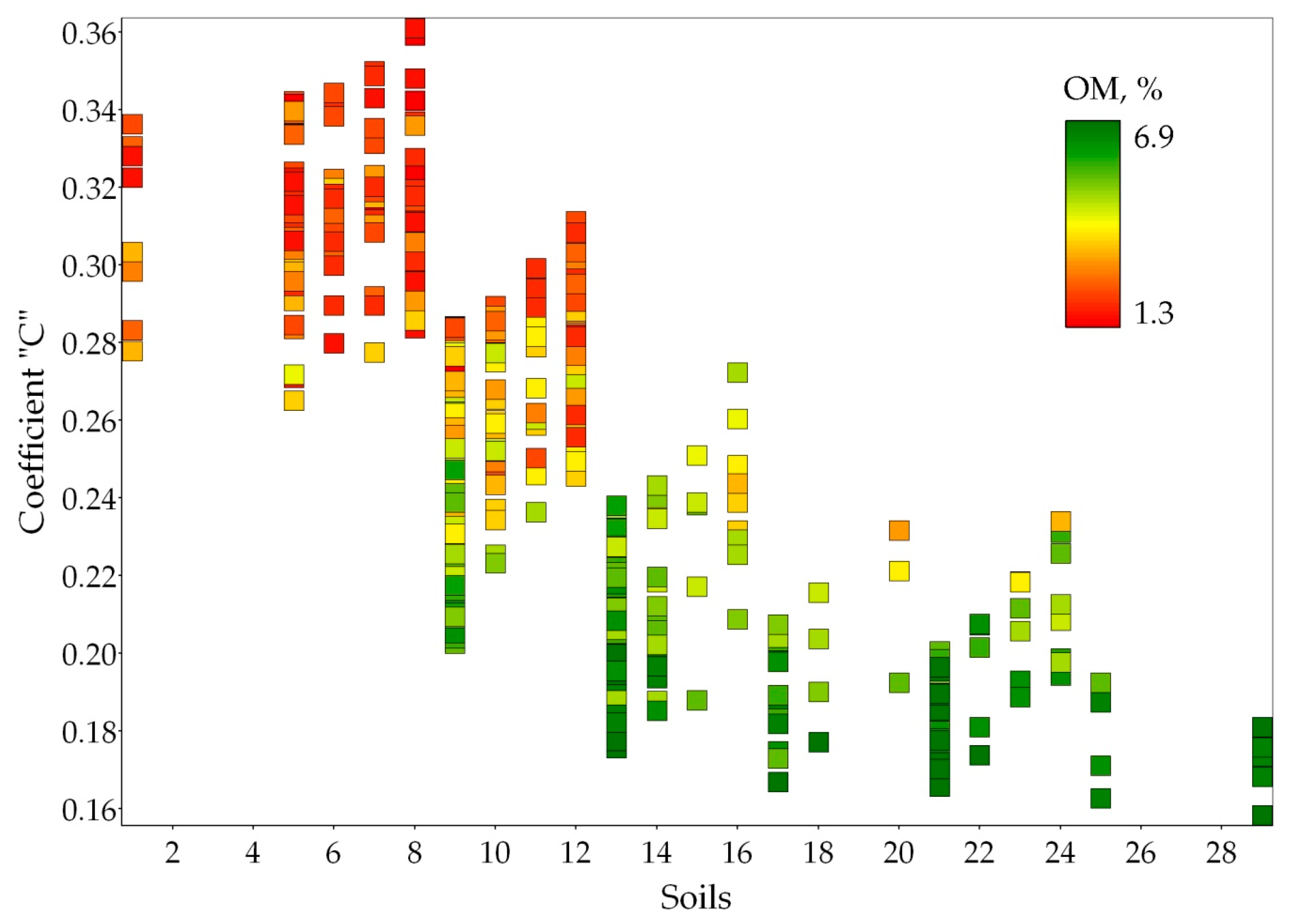
Erosion reduces the thickness of, or completely eliminates the upper soil horizons. Since the top soil layer contains the greatest amount of nutrients, erosion reduces the content of OM in the upper horizons, which, in turn, increases reflectivity [52,123] (Figure 6). The overall effect of OM content on spectral reflectivity is shown in the polynomial ladder (Figure 7). Each erosion step of the polynomial ladder contains less OM than the zonal step. However, the spectral characteristics also show the same effect (Figure 5).
Figure 6.
Dependence of the coefficient “C” of the MSL on the content of OM. Soil types are indicated by color and names are given in Table 1.
Figure 7.
Polynomial ladder. Multitemporal spectral characteristics of soils at 488 survey points and OM content (soil names are given in Table 1).
For example, the average value of OM content (Table 1) of gray forest soil is 3.42%, the average value of slightly eroded gray forest soil is 2.89%, moderately eroded soil—2.82%, and strongly eroded soil—2.52%. A similar series, but with an inverse relationship, is formed by the values of the coefficient “C” of the MSL—0.2476, 0.2613, 0.2773, and 0.2812. Thus, the OM content, as a characteristic of soil type [131], influences reflectivity by forming a polynomial (Figure 6). Soil erosion, by reducing the OM content for each soil type, forms deviations from the polynomial—a ladder (Figure 7).
Undoubtedly, even the average SCBSS are influenced not only by OM, but also by the particle size distribution and parent material type. High correlation values between OM content and multitemporal spectral characteristics may be related to the interplay between soil type, particle size distribution, parent material, and OM content [139].
4.2. Multitemporal Spectral Characteristics and Ground-Based Survey Dates
This study describes the polynomial ladder effect (Figure 5 and Figure 7). The effect is described by comparing spectral data averages over 40 years and a modern survey. In a work of 2024 [123], for the studied area the comparisons were made between averaged multitemporal characteristics and ground-based surveys of different periods, including archival ones. In a 2025 study [124], the same problem was studied for a different area. The studies showed that the relationship between OM content and averaged spectral characteristics in the form of a polynomial (Figure 6) with high values of the determination coefficient is preserved for all known ground-based surveys. The influence of the type of ground-based survey and its date on the approximation quality continues to be investigated. Agrochemical surveys in the territory of the former USSR have been conducted using a unified methodology since 1961. With increased accessibility of this information to researchers, new results may be obtained on the influence of ground survey dates and identification of functional relationships with spectral characteristics.
4.3. On the Possibility of Dividing Soil Types and Subtypes Based on the Multitemporal SCBSS
Figure 4c shows an approximation of the ordinal scale of zonal soil types and their average multitemporal spectral characteristics. The very possibility of constructing such approximations and separating soil types and subtypes based on spectral characteristics was described in a 2023 paper [74]. However, in the 2023 work, no effect of erosion was observed in the spectral series of the studied soils, which simplified the task. Another paper of 2023 [5] studied the effect of erosion, but only on one soil type, which again simplified the study. A 2025 research [139] described an even more striking result (agate-like soil cover structures). However, the effect of erosion on these structures was minimal. Based on these three papers, in the present study, regressions were constructed only for a zonal series of soils at a single erosion degree.
4.4. Methods of Soil Erosion Mapping
The approach to the analysis of erosion distribution based on multitemporal spectral characteristics proposed in this study is novel, but in the same time is intended to complement existing erosion mapping methods by addressing their shortcomings:
- (1)
- Ground investigations with extrapolation from a topographic map.
The primary method for detecting soil erosion in Russia has been and remains the ground-based approach, which involves field surveys and excavation of soil pits. However, the labor–intensive nature of soil profiles digging precludes the creation of an erosion map by simply interpolating ground-based measurements (descriptions). Therefore, the 1973 methodology [21] suggests the use of large-scale topographic maps (1:10,000 or 1:25,000). Essentially, the topographic map is deciphered, where the slope parameters (length and inclination) of the arable land are determined based on the isolines density. Ground-based studies help establish a functional relationship between the manifestation of erosion processes and the isolines density. The method disadvantages are its labor intensity and the using of general hypothesis that erosion occurs uniformly across the entire slope with equal inclination.
- (2)
- Modeling using DEM.
The most common modern method for constructing maps of the erosion processes distribution is modeling based on the DEM analysis [140,141]. There are two publicly available DEM with a resolution of 30 m for the entire surface of the Earth [30,31]. The main drawback of this approach is similar to the previous one: the general hypothesis of uniform erosion processes with identical relief parameters.
- (3)
- Frequency filter method.
An alternative to modeling and ground-based surveys is the method of indicative botany. This method assumes that the average long-term depressed state of vegetation should correlate with the degree of degradation [6]. Indeed, the more frequently areas of low VIs values are observed in field fragments, the more likely they are degraded/eroded [35]. The main advantage of indicative botany over modeling is that it detects not hypothetical locations of erosion, but actual manifestations through their impact on plants. The main disadvantage of the method is that the suppression of agricultural crops, in addition to degradation, can be caused by the initial heterogeneity of the soil cover.
- (4)
- SCBSS.
Another alternative to models and ground-based methods is the analysis of the SCBSS [1,2,3,4]. As shown in this study, the spectral reflectivity of the BSS of eroded soils is generally higher than that of their non-eroded counterparts. The authors believe that the spectral brightness analysis method of the BSS [42] may become a new and promising approach for detecting erosion. Under homogeneous conditions for soils and particle size distribution, this method has yielded good results [6]. At one of the study sites, this method also made it possible to detect soil differences [74,139]. The limitations of this method are the subject of this paper. Within a single soil type, this method performs better results than those described above, but when different soil types occur in the same area, it is difficult to distinguish eroded soil types from non-eroded.
Summing up the above, the ideal method for erosion mapping has not yet been created.
4.5. Future Research Directions
The main drawback of analyzing the SCBSS is the overlap between the reflectivity of non-eroded soils of one type and eroded soils of another. However, since eroded soils are confined to specific relief positions, a synthesis of the two methods may be promising. In the first stage, identify areas with minimal slopes using a 30 m spatial resolution DEM and identify zonal soil types within them. For each non-eroded area, create a region of adjacent slopes where erosion of this particular soil type is likely. In these regions, it is necessary to identify alternating eroded and non-eroded variants of a zonal soil type. Combining all these regions can allow the creation of a soil erosion map.
5. Conclusions
In the area of zonal transition of the soil cover from sod-podzolic soils to chernozems, two clearly defined functional relationships are formed, determining the multitemporal spectral characteristics of the bare soil surface (SCBSS):
- A polynomial decrease in the SCBSS in the following series of non-eroded soil types: sod-podzolic, light gray forest, gray forest, and dark gray forest soils, podzolized chernozems, leached chernozems, typical chernozems, and meadow-chernozem.
- A nearly linear increase in the SCBSS for each zonal soil type in the following series of erosion manifestations: non-eroded, slightly eroded, moderately eroded, and strongly eroded soils.
The superposition of the two functional relationships forms a distribution in the form of a polynomial ladder, where the general trend of decreasing reflectance in the zonal series of soils is interrupted by a trend of increasing reflectance with erosion. The polynomial ladder describes well the influence of soil erosion on multitemporal SCBSS.
Supplementary Materials
The following supporting information can be downloaded at https://www.mdpi.com/article/10.3390/rs18071057/s1, Figure S1: Multitemporal plot of the RED–NIR values distribution for one point in an agricultural field and MSL coefficients.
Author Contributions
Conceptualization, D.R.; methodology, D.R.; software, P.K., A.R. and M.K.; validation, P.K.; formal analysis, A.R.; investigation, D.R.; resources, D.R.; data curation, A.R. and P.K.; writing—original draft preparation, D.R.; writing—review and editing, M.K.; visualization, P.K.; supervision, D.R.; project administration, D.R.; funding acquisition, D.R. All authors have read and agreed to the published version of the manuscript.
Funding
This work was supported by the Russian Science Foundation, project No. 22-17-00071-Π, https://rscf.ru/project/22-17-00071/ (accessed on 24 December 2025) and state assignment No. FGUR-2025-0001.
Data Availability Statement
Publicly available Landsat datasets were analyzed in this study. These data can be found here: http://earthexplorer.usgs.gov, accessed on 24 December 2025. The other data that support the findings of this study are available on request from the corresponding author.
Conflicts of Interest
The authors declare no conflicts of interest.
Abbreviations
The following abbreviations are used in this manuscript:
| ATCOR | Atmospheric and topographic correction |
| BRSD | Big remote sensing data |
| BSS | Bare soil surface |
| DEM | Digital elevation model |
| ERDAS | Earth Resource Development Assessment System |
| FAO | Food and Agriculture Organization of the United Nations |
| GIS | Geographic information system |
| GPS | Global positioning system |
| MSL | Multitemporal soil line |
| NDVI | Normalized difference vegetation index |
| OM | Organic matter |
| RSD | Remote sensing data |
| RUSLE | Revised Universal Soil Loss Equation |
| SCBSS | Spectral characteristics of the bare soil surface |
| SCS | Soil cover structure |
| SNSL | Spectral neighborhood of the soil line |
| SSM | State soil map |
| UAV | Unmanned aerial vehicle |
| USLE | Universal Soil Loss Equation |
| USSR | Union of Soviet Socialist Republics |
| VIs | Vegetation indices |
References
- Polovina, S.; Radić, B.; Ristić, R.; Milčanović, V. Application of Remote Sensing for Identifying Soil Erosion Processes on a Regional Scale: An Innovative Approach to Enhance the Erosion Potential Model. Remote Sens. 2024, 16, 2390. [Google Scholar] [CrossRef] [Scilit]
- Qi, L.; Shi, P.; Dvorakova, K.; Van Oost, K.; Sun, Q.; Yu, H.; van Wesemael, B. Detection of Soil Erosion Hotspots in the Croplands of a Typical Black Soil Region in Northeast China: Insights from Sentinel-2 Multispectral Remote Sensing. Remote Sens. 2023, 15, 1402. [Google Scholar] [CrossRef] [Scilit]
- Wang, S.; Xu, X.; Huang, L. Spatial and Temporal Variability of Soil Erosion in Northeast China from 2000 to 2020. Remote Sens. 2023, 15, 225. [Google Scholar] [CrossRef] [Scilit]
- Gallo, B.C.; Magalhães, P.S.G.; Demattê, J.A.M.; Cervi, W.R.; Carvalho, J.L.N.; Barbosa, L.C.; Bellinaso, H.; Mello, D.C.d.; Veloso, G.V.; Alves, M.R.; et al. Soil Erosion Satellite-Based Estimation in Cropland for Soil Conservation. Remote Sens. 2023, 15, 20. [Google Scholar] [CrossRef] [Scilit]
- Rukhovich, D.I.; Koroleva, P.V.; Rukhovich, A.D.; Komissarov, M.A. Informativeness of the Long-term Average Spectral Characteristics of the Bare Soil Surface for the Detection of Soil Cover Degradation with the Neural Network Filtering of Remote Sensing Data. Remote Sens. 2023, 15, 124. [Google Scholar] [CrossRef] [Scilit]
- Rukhovich, D.I.; Koroleva, P.V.; Kalinina, N.V.; Vilchevskaya, Y.V.; Suleiman, G.A.; Chernousenko, G.I. Detecting Degraded Arable Land on the Basis of Remote Sensing Big Data Analysis. Eurasian Soil Sci. 2021, 54, 161–175. [Google Scholar] [CrossRef] [Scilit]
- Arrouays, D.; Dawson, L. Soil Priorities Around the World—An Introduction. Geoderma Reg. 2022, 30, e00555. [Google Scholar] [CrossRef] [Scilit]
- Montanarella, L.; Pennock, D.J.; Mckenzie, N.; Badraoui, M.; Chude, V.; Baptista, I.; Mamo, T.; Yemefack, M.; Aulakh, M.S.; Yagi, K.; et al. World’s Soils are under Threat. Soil 2016, 2, 79–82. [Google Scholar] [CrossRef] [Scilit]
- Pimentel, D.; Burgess, M. Soil Erosion Threatens Food Production. Agriculture 2013, 3, 443–463. [Google Scholar] [CrossRef] [Scilit]
- Borrelli, P.; Robinson, D.A.; Fleischer, L.R.; Lugato, E.; Ballabio, C.; Alewell, C.; Meusburger, K.; Modugno, S.; Schütt, B.; Ferro, V.; et al. An Assessment of the Global Impact of 21st Century Land Use Change on Soil Erosion. Nat. Commun. 2017, 8, 2013. [Google Scholar] [CrossRef] [Scilit]
- Ceglar, A.; Crepinsek, Z.; Zupanc, V.; Kajfez-Bogataj, L. A Comparative Study of Rainfall Erosivity for Eastern and Western Slovenia. Acta Agric. Slov. 2008, 91, 331–341. [Google Scholar] [CrossRef] [Scilit]
- Panagos, P.; Borrelli, P.; Poesen, J.; Ballabio, C.; Lugato, E.; Meusburger, K.; Montanarella, L.; Alewell, C. The New Assessment of Soil Loss by Water Erosion in Europe. Environ. Sci. Policy 2015, 54, 438–447. [Google Scholar] [CrossRef] [Scilit]
- Panagos, P.; Borrelli, P.; Robinson, D. FAO Calls for Actions to Reduce Global Soil Erosion. Mitig. Adapt. Strateg. Glob. Change 2020, 25, 789–790. [Google Scholar] [CrossRef] [Scilit]
- Golosov, V.N.; Gennadiev, A.N.; Markelov, M.V.; Zhidkin, A.P.; Kovach, R.G.; Olson, K.R.; Chendev, Y.G. Spatial and Temporal Features of Soil Erosion in the Forest-steppe Zone of the East-European Plain. Eurasian Soil Sci. 2011, 44, 794–801. [Google Scholar] [CrossRef] [Scilit]
- Litvin, L.F.; Kiryukhina, Z.P.; Krasnov, S.F.; Dobrovol’skaya, N.G. Dynamics of Agricultural Soil Erosion in European Russia. Eurasian Soil Sci. 2017, 50, 1343–1352. [Google Scholar] [CrossRef] [Scilit]
- Maltsev, K.; Yermolaev, O. Assessment of Soil Loss by Water Erosion in Small River Basins in Russia. Catena 2020, 195, 104726. [Google Scholar] [CrossRef] [Scilit]
- Zhidkin, A.P.; Komissarov, M.A.; Shamshurina, E.N.; Mishchenko, A.V. Soil Erosion in the Central Russian Upland: A Review. Eurasian Soil Sci. 2023, 56, 226–237. [Google Scholar] [CrossRef] [Scilit]
- Tuchkova, L.E.; Verkhovets, I.A.; Chuvashova, E.S.; Tikhoykina, I.M. Development of Systems of Measures to Protect Soils from Erosion by Example SPK “Victory of October” Hotynetskogo District, Oryol Region. Bull. Technosphere Saf. Rural Dev. 2020, 2, 44–47. (In Russian). Available online: https://cyberleninka.ru/article/n/razrabotka-sistem-meropriyatiy-po-zaschite-pochv-ot-erozii-na-primere-spk-pobeda-oktyabrya-hotynetskogo-rayona-orlovskoy-oblasti (accessed on 24 December 2025).
- Kozmenko, A.S. Combating Soil Erosion; Selkhozgiz: Moscow, Russia, 1973. (In Russian) [Google Scholar]
- Ischenko, T.A. (Ed.) All-Union Instruction on Soil Surveys and the Compilation of Large-Scale Soil Land Use Maps; Kolos: Moscow, Russia, 1973. (In Russian) [Google Scholar]
- Ivanekha, T.L.; Studennikov, N.A. The State of Soils in Farms of the Oryol Region and Measures of State Support for Soil Fertility. Bull. Rural Dev. Soc. Policy 2017, 4, 40–43. (In Russian). Available online: https://cyberleninka.ru/article/n/sostoyanie-pochv-v-hozyaystvah-orlovskoy-oblasti-i-mery-gosudarstvennoy-podderzhki-plodorodiya-pochv/viewer (accessed on 24 December 2025).
- Alewell, C.; Borrelli, P.; Meusburger, K.; Panagos, P. Using the USLE: Chances, Challenges and Limitations of Soil Erosion Modelling. Int. Soil Water Conserv. Res. 2019, 7, 203–225. [Google Scholar] [CrossRef] [Scilit]
- Rousseva, S.; Stoynova, V.; Lozanova, L.; Malinov, I.; Tcvetkova, E.; Dzhodzhov, C.; Kroumov, V.; Mitova, M.; Ilieva, D. Factors and Risk of Soil Erosion by Water and Wind in the Zone of Bulgarian Chernozems. 2017. Available online: https://www.academia.edu/114107431/Factors_and_Risk_of_Soil_Erosion_by_Water_and_Wind_in_the_Zone_of_Bulgarian_Chernozems (accessed on 24 December 2025).
- Patriche, C.V. Applying RUSLE for Soil Erosion Estimation in Romania under Current and Future Climate Scenarios. Geoderma Reg. 2023, 34, e00687. [Google Scholar] [CrossRef] [Scilit]
- Pásztor, L.; Waltner, I.; Centeri, C.; Belényesi, M.; Takács, K. Soil Erosion of Hungary Assessed by Spatially Explicit Modelling. J. Maps 2016, 12, 407–414. [Google Scholar] [CrossRef] [Scilit]
- Devátý, J.; Dostál, T.; Hösl, R.; Krása, J.; Strauss, P. Effects of Historical Land Use and Land Pattern Changes on Soil Erosion—Case Studies from Lower Austria and Central Bohemia. Land Use Policy 2019, 82, 674–685. [Google Scholar] [CrossRef] [Scilit]
- Tsymbarovich, P.; German, K.; Kumani, M.; Golosov, V.N.; Andreeva, O.V. Soil Erosion: An Important Indicator for the Assessment of Land Degradation Neutrality in Russia. Int. Soil Water Conserv. Res. 2021, 8, 418–429. [Google Scholar] [CrossRef] [Scilit]
- Haiyan, F.; Liying, S. Modelling Soil Erosion and its Response to the Soil Conservation Measures in the Black Soil Catchment, Northeastern China. Soil Tillage Res. 2017, 165, 23–33. [Google Scholar] [CrossRef] [Scilit]
- Fang, H.; Fan, Z. Assessment of Soil Erosion at Multiple Spatial Scales Following Land Use Changes in 1980–2017 in the Black Soil Region, (NE) China. Int. J. Environ. Res. Public Health 2020, 17, 7378. [Google Scholar] [CrossRef] [Scilit] [PubMed]
- SRTM. Available online: http://srtm.csi.cgiar.org (accessed on 24 December 2025).
- European Space Agency. Copernicus Global Digital Elevation Model; Distributed by Open Topography; European Space Agency: Paris, France, 2021. [Google Scholar] [CrossRef]
- Wischmeier, W.H.; Smith, D.D. Predicting Rainfall Erosion Losses: A Guide to Conservation Planning; USDA: Washington, DC, USA, 1978. [Google Scholar]
- Renard, K.G.; Foster, G.R.; Weesies, G.A.; Mccool, D.K.; Yoder, D.C. Predicting Soil Erosion by Water: A Guide to Conservation Planning with the Revised Universal Soil Loss Equation (RUSLE); U.S. Department of Agriculture: Washington, DC, USA, 1997; ISBN 0160489385.
- Rukhovich, D.I.; Koroleva, P.V.; Rukhovich, D.D.; Rukhovich, A.D. Recognition of the Bare Soil Using Deep Machine Learning Methods to Create Maps of Arable Soil Degradation Based on the Analysis of Multi-temporal Remote Sensing Data. Remote Sens. 2022, 14, 2224. [Google Scholar] [CrossRef] [Scilit]
- Rukhovich, D.I.; Koroleva, P.V.; Rukhovich, D.D.; Kalinina, N.V. The Use of Deep Machine Learning for the Automated Selection of Remote Sensing Data for the Determination of Areas of Arable Land Degradation Processes Distribution. Remote Sens. 2021, 13, 155. [Google Scholar] [CrossRef] [Scilit]
- Khitrov, N.B.; Rukhovich, D.I.; Koroleva, P.V.; Kalinina, N.V.; Trubnikov, A.V.; Petukhov, D.A.; Kulyanitsa, A.L. A Study of the Responsiveness of Crops to Fertilizers by Zones of Stable Intra-field Heterogeneity Based on Big Satellite Data Analysis. Arch. Agron. Soil Sci. 2020, 66, 1963–1975. [Google Scholar] [CrossRef] [Scilit]
- Winzeler, H.E.; Mancini, M.; Blackstock, J.M.; Libohova, Z.; Owens, P.R.; Ashworth, A.J.; Miller, D.M.; Silva, S.H.G. Vegetation Masking of Remote Sensing Data Aids Machine Learning for Soil Fertility Prediction. Remote Sens. 2024, 16, 3297. [Google Scholar] [CrossRef] [Scilit]
- Samarinas, N.; Tsakiridis, N.L.; Kokkas, S.; Kalopesa, E.; Zalidis, G.C. Soil Data Cube and Artificial Intelligence Techniques for Generating National-Scale Topsoil Thematic Maps: A Case Study in Lithuanian Croplands. Remote Sens. 2023, 15, 5304. [Google Scholar] [CrossRef] [Scilit]
- Berman, M. Confidence Intervals and Regions for Proportions under Various Three-Endmember Linear Mixture Models. Remote Sens. 2023, 15, 2733. [Google Scholar] [CrossRef] [Scilit]
- Urbina-Salazar, D.; Vaudour, E.; Richer-de-Forges, A.C.; Chen, S.; Martelet, G.; Baghdadi, N.; Arrouays, D. Sentinel-2 and Sentinel-1 Bare Soil Temporal Mosaics of 6-Year Periods for Soil Organic Carbon Content Mapping in Central France. Remote Sens. 2023, 15, 2410. [Google Scholar] [CrossRef] [Scilit]
- He, C.; Liu, Y.; Wang, D.; Liu, S.; Yu, L.; Ren, Y. Automatic Extraction of Bare Soil Land from High-Resolution Remote Sensing Images Based on Semantic Segmentation with Deep Learning. Remote Sens. 2023, 15, 1646. [Google Scholar] [CrossRef] [Scilit]
- Koroleva, P.V.; Rukhovich, D.I.; Rukhovich, A.D.; Rukhovich, D.D.; Kulyanitsa, A.L.; Trubnikov, A.V.; Kalinina, N.V.; Simakova, M.S. Location of Bare Soil Surface and Soil Line on the RED–NIR Spectral Plane. Eurasian Soil Sci. 2017, 50, 1375–1385. [Google Scholar] [CrossRef] [Scilit]
- Delaney, B.; Tansey, K.; Whelan, M. Satellite Remote Sensing Techniques and Limitations for Identifying Bare Soil. Remote Sens. 2025, 17, 630. [Google Scholar] [CrossRef] [Scilit]
- Rukhovich, D.I.; Rukhovich, A.D.; Simakova, M.S.; Kulyanitsa, A.L.; Koroleva, P.V.; Rukhovich, D.D. Application of the Spectral Neighborhood of Soil Line Technique to Analyze the Intensity of Soil Use in 1985–2014 (by the Example of Three Districts of Tula Oblast). Eurasian Soil Sci. 2018, 51, 345–358. [Google Scholar] [CrossRef] [Scilit]
- Kulyanitsa, A.L.; Rukhovich, A.D.; Rukhovich, D.D.; Koroleva, P.V.; Rukhovich, D.I.; Simakova, M.S. The Application of the Piecewise Linear Approximation to the Spectral Neighborhood of Soil Line for the Analysis of the Quality of Normalization of Remote Sensing Materials. Eurasian Soil Sci. 2017, 50, 387–395. [Google Scholar] [CrossRef] [Scilit]
- Bowers, S.A.; Hanks, R.J. Reflection of Radiant Energy from Soils. Soil Sci. 1965, 100, 130–138. [Google Scholar] [CrossRef] [Scilit]
- Karmanov, I.I. On the Application of Spectrophotometric Coefficients to the Study of Soil-forming Processes. Pochvovedeniye 1968, 2, 13. (In Russian) [Google Scholar]
- Karmanov, I.I. Spectral Reflectance and Color of Soils as Indicators of their Properties; Kolos: Moscow, Russia, 1974. (In Russian) [Google Scholar]
- Sinha, A.K. Spectral Reflectance Characteristics of Soil and its Correlation with Soil Properties and Surface Conditions. J. Indian Soc. Remote Sens. 1986, 14, 1–9. [Google Scholar] [CrossRef] [Scilit]
- Coleman, T.L.; Agbu, P.A.; Montgomery, O.L. Spectral Differentiation on Surface Soils and Soil Properties: Is it Possible from Space Platforms? Soil Sci. 1993, 155, 283–293. [Google Scholar] [CrossRef] [Scilit]
- Barnes, E.M.; Baker, M.G. Multispectral Data for Mapping Soil Texture: Possibilities and Limitations. Appl. Eng. Agric. 1999, 16, 731–741. [Google Scholar] [CrossRef] [Scilit]
- Orlov, D.S.; Sukhanova, N.I.; Rozanova, M.S. Spectral Reflectance of Soils and their Components; Moscow State University: Moscow, Russia, 2001. (In Russian) [Google Scholar]
- Fox, G.A.; Sabbagh, G.J. Estimation of Soil Organic Matter from Red and Near-infrared Remotely Sensed Data Using a Soil Line Euclidean Distance Technique. Soil Sci. Soc. Am. J. 2002, 66, 1922–1928. [Google Scholar] [CrossRef] [Scilit]
- Barnes, E.M.; Sudduth, K.A.; Hummel, J.; Lesch, S.M.; Corwin, D.L.; Yang, C.; Daughtry, C.S.; Bausch, W.C. Remote- and ground-based Sensor Techniques to Map Soil Properties. Photogramm. Eng. Remote Sens. 2003, 69, 619–630. [Google Scholar] [CrossRef] [Scilit]
- Brown, D.J.; Shepherd, K.D.; Walsh, M.G.; Mays, M.D.; Reinsch, T.G. Global Soil Characterization with VNIR Diffuse Reflectance Spectroscopy. Geoderma 2006, 132, 273–290. [Google Scholar] [CrossRef] [Scilit]
- Metternicht, G.; Zinck, J.A. Remote Sensing of Soil Salinization: Impact on Land Management; CRC Press: New York, NY, USA, 2009. [Google Scholar]
- Khitrov, N.B.; Rukhovivh, D.I.; Kalinina, N.V.; Novikova, A.F.; Pankova, E.I.; Chernousenko, G.I. Estimation of the Areas of Salt-affected Soils in the European Part of Russia on the Basis of a Digital Map of Soil Salinization on a Scale of 1:2.5 M. Eurasian Soil Sci. 2009, 42, 581–590. [Google Scholar] [CrossRef] [Scilit]
- Lesaignoux, A.; Fabre, S.; Briotter, X.; Olioso, A. Soil Moisture Impact on Lab Measured Reflectance of Bare Soils in the Optical Domain [0.4–15 μM]. In 2009 IEEE International Geoscience and Remote Sensing Symposium; IEEE: Piscataway, NJ, USA, 2009. [Google Scholar] [CrossRef] [Scilit]
- Chernousenko, G.I.; Kalinina, N.V.; Khitrov, N.B.; Pankova, E.I.; Rukhovich, D.I.; Yamnova, I.A.; Novikova, A.F. Quantification of the Areas of Saline and Solonetzic Soils in the Ural Federal Region of the Russian Federation. Eurasian Soil Sci. 2011, 44, 367–379. [Google Scholar] [CrossRef] [Scilit]
- Ben-Dor, E.; Irons, J.R.; Epema, G.F. Soil reflectante. In Manual of Remote Sensing: Remote Sensing for Earth Science; Rencz, A.N., Ryerson, R.A., Eds.; John Wiley & Sons: New York, NY, USA, 1999; pp. 111–187. [Google Scholar]
- Clark, R.N. Spectroscopy of Rocks and Minerals, and Principles of Spectroscopy. In Manual of Remote Sensing; Rencz, A., Ed.; John Wiley and Sons: New York, NY, USA, 1999; pp. 3–58. [Google Scholar]
- Malley, D.F.; Martin, P.D.; McClintock, L.M.; Yesmin, L.; Eilers, R.G.; Haluschak, P. Feasibility of Analysing Archived Canadian Prairie Agricultural Soils by Near Infrared Reflectance Spectroscopy. In Near Infrared Spectroscopy: Proceedings of the 9th International Conference; NIR Publications: Chichester, UK, 2000; pp. 579–585. [Google Scholar]
- Chang, C.W.; Laird, D.A.; Mausbach, M.J.; Hurburgh, C.R. Near-infrared Reflectance Spectroscopy-principal Components Regression Analyses of Soil Properties. Soil Sci. Soc. Am. J. 2001, 65, 480–490. [Google Scholar] [CrossRef] [Scilit]
- Shepherd, K.D.; Walsh, M.G. Development of Reflectance Spectral Libraries for Characterization of Soil Properties. Soil Sci. Soc. Am. J. 2002, 66, 988–998. [Google Scholar] [CrossRef]
- Brown, D.J. Using a global VNIR Soil-spectral Library for Local Soil Characterization and Landscape Modeling in a 2nd-order Uganda Watershed. Geoderma 2007, 140, 444–453. [Google Scholar] [CrossRef] [Scilit]
- Sankey, J.B.; Brown, D.J.; Bernard, M.L.; Lawrence, R.L. Comparing Local vs. Global Visible and Near-infrared (VisNIR) Diffuse Reflectance Spectroscopy (DRS) Calibrations for the Prediction of Soil Clay, Organic C and Inorganic C. Geoderma 2008, 148, 149–158. [Google Scholar] [CrossRef] [Scilit]
- Belinaso, H.; Demattê, J.A.M.; Remerio, S.A. Soil Spectral Library and its Use in Soil Classification. Rev. Bras. Cienc. Solo 2010, 34, 861–870. [Google Scholar] [CrossRef] [Scilit]
- Knadel, M.; Deng, F.; Thomsen, A.; Greve, M.H. Development of a Danish National Vis-NIR Soil Spectral Library for Soil Organic Carbon Determination. In Digital Soil Assessments and Beyond: Proceedings of the 5th Global Workshop on Digital Soil Mapping, Sydney, Australia; CRC Press: London, UK, 2012; pp. 403–408. Available online: https://pure.au.dk/portal/en/publications/development-of-a-danish-national-visnir-soil-spectral-library-for-2/ (accessed on 20 March 2026).
- Rossel, R.A.; Webster, R. Predicting Soil Properties from the Australian Soil Visible–Near Infrared Spectroscopic Database. Eur. J. Soil Sci. 2012, 63, 848–860. [Google Scholar] [CrossRef] [Scilit]
- Stevens, A.; Nocita, M.; Tóth, G.; Montanarella, L.; van Wesemael, B. Prediction of Soil Organic Carbon at the European Scale by Visible and Near InfraRed Reflectance Spectroscopy. PLoS ONE 2013, 8, e66409. [Google Scholar] [CrossRef] [Scilit]
- Shi, Z.; Ji, W.; Viscarra Rossel, R.A.; Chen, S.; Zhou, Y. Prediction of Soil Organic Matter Using a Spatially Constrained Local Partial Least Squares Regression and the Chinese vis-NIR Spectral Library. Eur. J. Soil Sci. 2015, 66, 679–687. [Google Scholar] [CrossRef] [Scilit]
- Gogé, F.; Gomez, C.; Jolivet, C.; Joffre, R. Which Strategy is Best to Predict Soil Properties of a Local Site from a National Vis-NIR Database? Geoderma 2014, 213, 1–9. [Google Scholar] [CrossRef] [Scilit]
- Zanini, M.; Heiden, U.; Pace, L.; Casa, R.; Priori, S. Soil Reflectance Composite for Digital Soil Mapping in a Mediterranean Cropland District. Remote Sens. 2025, 17, 89. [Google Scholar] [CrossRef] [Scilit]
- Rukhovich, D.I.; Koroleva, P.V.; Rukhovich, A.D.; Komissarov, M.A. Updating of the Archival Large-Scale Soil Map Based on the Multitemporal Spectral Characteristics of the Bare Soil Surface Landsat Scenes. Remote Sens. 2023, 15, 4491. [Google Scholar] [CrossRef] [Scilit]
- Zhao, R.; Yu, W.; Deng, X.; Huang, Y.; Yang, W.; Zhou, W. Analysis of Land Surface Performance Differences and Uncertainty in Multiple Versions of MODIS LST Products. Remote Sens. 2024, 16, 4255. [Google Scholar] [CrossRef] [Scilit]
- Tao, L.; Di, Y.; Wang, Y.; Ryu, D. Normalized Temperature Drought Index (NTDI) for Soil Moisture Monitoring Using MODIS and Landsat-8 Data. Remote Sens. 2023, 15, 2830. [Google Scholar] [CrossRef] [Scilit]
- Wang, Z.; Wu, W.; Liu, H. Spatial Estimation of Soil Organic Carbon Content Utilizing PlanetScope, Sentinel-2, and Sentinel-1 Data. Remote Sens. 2024, 16, 3268. [Google Scholar] [CrossRef] [Scilit]
- Li, X.; Wen, H.; Xing, Z.; Cheng, L.; Wang, D.; Wang, M. Mapping Topsoil Carbon Storage Dynamics of Croplands Based on Temporal Mosaicking Images of Landsat and Machine Learning Approach. Remote Sens. 2024, 16, 2010. [Google Scholar] [CrossRef] [Scilit]
- Zayani, H.; Fouad, Y.; Michot, D.; Kassouk, Z.; Baghdadi, N.; Vaudour, E.; Lili-Chabaane, Z.; Walter, C. Using Machine-Learning Algorithms to Predict Soil Organic Carbon Content from Combined Remote Sensing Imagery and Laboratory Vis-NIR Spectral Datasets. Remote Sens. 2023, 15, 4264. [Google Scholar] [CrossRef] [Scilit]
- Ma, H.; Wang, C.; Liu, J.; Wang, X.; Zhang, F.; Yuan, Z.; Yao, C.; Pan, X. A Framework for Retrieving Soil Organic Matter by Coupling Multi-Temporal Remote Sensing Images and Variable Selection in the Sanjiang Plain, China. Remote Sens. 2023, 15, 3191. [Google Scholar] [CrossRef] [Scilit]
- He, C.; Wang, Q.; Yang, J.; Xu, W.; Yuan, B. BLEI: Research on a Novel Remote Sensing Bare Land Extraction Index. Remote Sens. 2024, 16, 1534. [Google Scholar] [CrossRef] [Scilit]
- Zhang, H.; Fu, X.; Zhang, Y.; Qi, Z.; Zhang, H.; Xu, Z. Mapping Multi-Depth Soil Salinity Using Remote Sensing-Enabled Machine Learning in the Yellow River Delta, China. Remote Sens. 2023, 15, 5640. [Google Scholar] [CrossRef] [Scilit]
- Rasooli, N.; Mirzaei, S.; Pignatti, S. Monitoring Gypsiferous Soils by Leveraging Advanced Spaceborne Hyperspectral Imagery via Spectral Indices and a Machine Learning Approach. Remote Sens. 2025, 17, 1914. [Google Scholar] [CrossRef] [Scilit]
- Gorokhova, I.N.; Tarnopolsky, L.A.; Khitrov, N.B.; Kruglyakova, N.G. Mapping of Surface-Effervescing Soils of Arable Lands in the South of the Volga Upland. Eurasian Soil Sci. 2025, 58, 117. [Google Scholar] [CrossRef] [Scilit]
- George, E.B.; Gomez, C.; Kumar, N.D. Adapting Prediction Models to Bare Soil Fractional Cover for Extending Topsoil Clay Content Mapping Based on AVIRIS-NG Hyperspectral Data. Remote Sens. 2024, 16, 1066. [Google Scholar] [CrossRef] [Scilit]
- Shashko, D.I.; Nosov, S.I.; Loiko, P.F. Natural and Agricultural Zoning of the Land Fund of the USSR, Scale 1:8,000,000; GUGK: Moscow, Russia, 1984. [Google Scholar]
- Dobrovolsky, G.V.; Urusevskaya, I.S.; Rozov, N.N. Map of Soil-Geographical Zoning of the USSR, Scale 1: 8000000; GUGK: Moscow, Russia, 1983. [Google Scholar]
- Rukhovich, D.I.; Koroleva, P.V.; Kalinina, N.V.; Vil’chevskaya, E.V.; Simakova, M.S.; Dolinina, E.A.; Rukhovich, S.V. State Soil Map of the Russian Federation: An ArcInfo version. Eurasian Soil Sci. 2013, 46, 225–240. [Google Scholar] [CrossRef] [Scilit]
- Bulgakov, D.S.; Rukhovich, D.I.; Shishkonakova, E.A.; Vil’chevskaya, E.V. Separation of Agroclimatic Areas for Optimal Crop Growing within the Framework of the Natural–Agricultural Zoning of Russia. Eurasian Soil Sci. 2016, 49, 1049–1060. [Google Scholar] [CrossRef] [Scilit]
- Rukhovich, D.I.; Koroleva, P.V.; Vilchevskaya, E.V.; Kalinina, N.V. Digital Thematic Cartography as a Change in the Available Primary Sources and Ways of Using them. In Digital Soil Mapping: Theoretical and Experimental Studies; Ivanov, A.L., Sorokina, N.P., Savin, I.Y., Eds.; Dokuchaev Soil Science Institute: Moscow, Russia, 2012; pp. 58–86. [Google Scholar]
- Landsat Data Courtesy of the U.S. Geological Survey. 2023. Available online: https://earthexplorer.usgs.gov (accessed on 24 December 2025).
- Modified Copernicus Sentinel Data 2016–2023. Available online: https://www.sentinel-hub.com (accessed on 24 December 2025).
- USGS EROS Archive—Declassified Data-Declassified Satellite Imagery-1. Available online: https://www.usgs.gov/centers/eros/science/usgs-eros-archive-declassified-data-declassified-satellite-imagery-1?qt-science_center_objects=0#qt-science_center_objects (accessed on 24 December 2025).
- Erdas Imagine. Available online: https://www.hexagongeospatial.com/products/power-portfolio/erdas-imagine (accessed on 24 December 2025).
- Liu, P.; Di, L.; Du, Q.; Wang, L. Remote Sensing Big Data: Theory, Methods and Applications. Remote Sens. 2018, 10, 711. [Google Scholar] [CrossRef] [Scilit]
- Chen, A. Carbonaceous Aerosols and Climate Change How Researchers Proved That Black Carbon is a Significant Force in the Atmosphere. EETD Newsl. 2004, 5. Available online: https://web.archive.org/web/20160304051425/http://eetd.lbl.gov/newsletter/nl17/eetd-nl17-4-blackcarbon.html (accessed on 24 December 2025).
- Mitchell, J.M. Visual Range in the Polar Regions with Particular References to the Alaskan Arctic. J. Atmos. Terr. Phys. Spec. 1957, 1, 195–211. [Google Scholar]
- McCarty, J.L.; Ellicott, E.A.; Romanenkov, V.; Rukhovitch, D.; Koroleva, P. Multi-year Black Carbon Emissions from Cropland Burning in the Russian Federation. Atmos. Environ. 2012, 63, 223–238. [Google Scholar] [CrossRef] [Scilit]
- Kauth, R.J.; Thomas, G.S. The tasseled cap—A Graphic Description of the Spectral-temporal Development of Agricultural Crops as Seen by LANDSAT. In Proceedings of the Symposium on Machine Processing of Remotely Sensed Data, Purdue University, West Lafayette, IN, USA, 29 June–1 July 1976; (A77-15051 04-43); Institute of Electrical and Electronics Engineers, Inc.: New York, NY, USA, 1976; pp. 4B-41–4B-51. [Google Scholar]
- Crist, E.P.; Cicone, R.C. A Physically-based Transformation of Thematic Mapper Data—The TM Tasseled Cap. IEEE Trans. Geosci. Remote Sens. 1984, GE-22, 256–263. [Google Scholar] [CrossRef] [Scilit]
- Pearson, K. LIII. On Lines and Planes of Closest Fit to Systems of Points in Space. Lond. Edinb. Dublin Philos. Mag. J. Sci. 1901, 2, 559–572. [Google Scholar] [CrossRef] [Scilit]
- Rukhovich, D.I. Method for Creating Soil Maps Based on the Results of the Analysis of Remote Sensing Data. Patent RU 2777272 C1, IPC G01V 9/00, 1 August 2022.
- Rouse, J.W.; Haas, R.H.; Schell, J.A.; Deering, D.W. Monitoring Vegetation Systems in the Great Plains with ERTS. In Proceedings of the Third ERTS Symposium, Washington, DC, USA, 10–14 December 1973; Scientific and Technical Information Office, NASA: Washington, DC, USA, 1974; Volume 1, pp. 309–317. [Google Scholar]
- Zhang, J.; Zhu, H.; Wang, P.; Ling, X. ATT Squeeze U-Net: A Lightweight Network for Forest Fire Detection and Recognition. IEEE Access 2021, 9, 10858–10870. [Google Scholar] [CrossRef] [Scilit]
- Ioffe, S.; Szegedy, C. Batch Normalization: Accelerating Deep Network Training by Reducing Internal Covariate Shift. arXiv 2015, arXiv:1502.03167v3. [Google Scholar] [CrossRef] [Scilit]
- Jadon, S. A Survey of Loss Functions for Semantic Segmentation. In Proceedings of the 2020 IEEE Conference on Computational Intelligence in Bioinformatics and Computational Biology (CIBCB), Santiago, Chile, 27–29 October 2020; IEEE: Piscataway, NJ, USA, 2020; pp. 1–7. [Google Scholar] [CrossRef] [Scilit]
- Kingma, D.P.; Ba, J. Adam: A Method for Stochastic Optimization. arXiv 2014, arXiv:1412.6980. Available online: https://arxiv.org/abs/1412.6980 (accessed on 24 December 2025).
- Friedman, J.H. Greedy Function Approximation: A Gradient Boosting Machine. Ann. Stat. 2001, 29, 1189–1232. [Google Scholar] [CrossRef] [Scilit]
- Prokhorenkova, L.; Gusev, G.; Vorobev, A.; Dorogush, A.V.; Gulin, A. Catboost: Unbiased Boosting with Categorical Features. Adv. Neural Inf. Process. Syst. 2018, 31, 6638–6648. [Google Scholar]
- Python. Available online: https://www.python.org/ (accessed on 24 December 2025).
- LeCun, Y.; Bottou, L.; Bengio, Y.; Haffner, P. Gradient-based Learning Applied to Document Recognition. Proc. IEEE 1998, 86, 2278–2324. [Google Scholar] [CrossRef] [Scilit]
- Krizhevsky, A.; Sutskever, I.; Hinton, G.E. Imagenet Classification with Deep Convolutional Neural Networks. Adv. Neural Inf. Process. Syst. 2012, 25, 1097–1105. [Google Scholar] [CrossRef] [Scilit]
- Lyuri, D.I.; Goryachkin, S.V.; Karavaeva, N.A.; Denisenko, E.A.; Nefedova, T.G. Dynamics of Agricultural Lands of Russia in the 20th Century and Post-agrogenic Restoration of Vegetation and Soils; GEOS: Moscow, Russia, 2010. (In Russian) [Google Scholar]
- Rukhovich, D.I.; Koroleva, P.V.; Shapovalov, D.A.; Komissarov, M.A.; Pham, T.G. Transformation of Arable Lands in Russia over Last Half Century—Analysis Based on Detailed Mapping and Retrospective Monitoring of Soil–Land Cover and Decipherment of Big Remote Sensing Data. Sustainability 2025, 17, 6203. [Google Scholar] [CrossRef] [Scilit]
- Zhidkin, A.P.; Rukhovich, D.I.; Maltsev, K.A.; Koroleva, P.V. Variation of Soil Erosion Estimates Based on Different Maps of Cropland in Belgorod Oblast, Russia. Eurasian Soil Sci. 2024, 57, 666–676. [Google Scholar] [CrossRef] [Scilit]
- Bryzzhev, A.V.; Rukhovich, D.I.; Koroleva, P.V.; Kalinina, N.V.; Vilchevskaya, E.V.; Dolinina, E.A.; Rukhovich, S.V. Organization of Retrospective Monitoring of the Soil Cover in Azov district of Rostov Oblast. Eurasian Soil Sci. 2015, 48, 1029–1049. [Google Scholar] [CrossRef] [Scilit]
- Shapovalov, D.A.; Koroleva, P.V.; Kalinina, N.V.; Rukhovich, D.I.; Suleiman, G.A.; Dolinina, E.A. Differences in Inventories of Waterlogged Territories in Soil Surveys of Different Years and in Land Management Documents. Eurasian Soil Sci. 2020, 53, 294–309. [Google Scholar] [CrossRef] [Scilit]
- Rukhovich, D.I.; Simakova, M.S.; Kulyanitsa, A.L.; Bryzzhev, A.V.; Koroleva, P.V.; Kalinina, N.V.; Vil’Chevskaya, E.V.; Dolinina, E.A.; Rukhovich, S.V. Impact of Shelterbelts on the Fragmentation of Erosional Networks and Local Soil Waterlogging. Eurasian Soil Sci. 2014, 47, 1086–1099. [Google Scholar] [CrossRef] [Scilit]
- Rukhovich, D.I.; Simakova, M.S.; Kulyanitsa, A.L.; Bryzzhev, A.V.; Koroleva, P.V.; Kalinina, N.V.; Vil’Chveskaya, E.V.; Dolinina, E.A.; Rukhovich, S.V. Retrospective Analysis of Changes in Land Uses on Vertic Soils of Closed Mesodepressions on the Azov Plain. Eurasian Soil Sci. 2015, 48, 1050–1075. [Google Scholar] [CrossRef] [Scilit]
- Rukhovich, D.I.; Simakova, M.S.; Kulyanitsa, A.L.; Bryzzhev, A.V.; Koroleva, P.V.; Kalinina, N.V.; Chernousenko, G.I.; Vil’Chevskaya, E.V.; Dolinina, E.A.; Rukhovich, S.V. Methodology for Comparing Soil Maps of Different Dates with the Aim to Reveal and Describe Changes in the Soil Cover (by the Example of Soil Salinization Monitoring). Eurasian Soil Sci. 2016, 49, 145–162. [Google Scholar] [CrossRef] [Scilit]
- Rukhovich, D.I.; Simakova, M.S.; Kulyanitsa, A.L.; Bryzzhev, A.V.; Koroleva, P.V.; Kalinina, N.V.; Chernousenko, G.I.; Vil’Chevskaya, E.V.; Dolinina, E.A. The Influence of Soil Salinization on Land Use Changes in Azov District of Rostov Oblast. Eurasian Soil Sci. 2017, 50, 276–295. [Google Scholar] [CrossRef] [Scilit]
- Koroleva, P.V.; Rukhovich, D.I.; Shapovalov, D.A.; Suleiman, G.A.; Dolinina, E.A. Retrospective Monitoring of Soil Waterlogging on Arable Land of Tambov Oblast in 2018–1968. Eurasian Soil Sci. 2019, 52, 834–852. [Google Scholar] [CrossRef] [Scilit]
- Rukhovich, D.; Koroleva, P.; Rukhovich, A.; Komissarov, M. A Detailed Mapping of Soil Organic Matter Content in Arable Land Based on the Multitemporal Soil Line Coefficients and Neural Network Filtering of Big Remote Sensing Data. Geoderma 2024, 447, 116941. [Google Scholar] [CrossRef] [Scilit]
- Rukhovich, D.I.; Borshchev, D.G.; Koroleva, P.V.; Rukhovich, A.D. Influence of Field Survey Principles on the Quality of Approximation of the Relationship Between the Soil Organic Matter Content and the Multitemporal Spectral Characteristics. Eurasian Soil Sci. 2025, 58, 105. [Google Scholar] [CrossRef] [Scilit]
- Maksimov, P.G.; Florinsky, M.A. Guidelines for Conducting a Comprehensive Agrochemical Survey of Soils on Agricultural Land; TsNTIPR: Moscow, Russia, 1994; (In Russian). Available online: https://files.stroyinf.ru/Data2/1/4293736/4293736617.pdf?ysclid=lsztcn25o122621490 (accessed on 24 December 2025).
- Soil Map of the Collective Farm Udarnik, Klyavlinsky District, Samara Region, Scale 1:25000; Roskomzem RosNIIzemproekt VolgoNIIgiprozem: Samara, Russia, 1995.
- Fridland, V.M. Structure of the Soil Mantle. Geoderma 1974, 12, 35–41. [Google Scholar] [CrossRef] [Scilit]
- Smith, G.D. A New Classification Scheme, Progress Report. In Proceedings of the 7th International Congress of Soil Science, Madison, WI, USA, 22–23 August 1960; Volume 4, pp. 111–150. [Google Scholar]
- Johnson, W.M. The Pedon and the Polypedon. Soil Sci. Soc. Am. J. 1963, 27, 212–215. [Google Scholar] [CrossRef] [Scilit]
- Arnold, R.; Blume, H.P.; Bockheim, J.; Boyadgiev, T.; Bridges, E.; Brinkman, R.; Broll, G.; Bronger, A.; Constantini, E.; Creutzberg, D.; et al. World Reference Base for Soil Resources: IUSS Working Group WRB. FAO; Food and Agriculture Organization of the United Nations Rome: Rome, Italy, 1998. [Google Scholar]
- Unified State Register of Soil Resources of Russia. Available online: http://egrpr.soil.msu.ru/index.php (accessed on 24 December 2025).
- State Standard of the USSR 26213-91; Soils. Methods for Determination of Organic Matter. USSR Committee for Standardization and Metrology: Moscow, Russia, 1993. Available online: https://meganorm.ru/Data2/1/4294828/4294828267.pdf (accessed on 24 December 2025).
- Walkley, A.J.; Black, I.A. Estimation of Soil Organic Carbon by the Chromic Acid Titration Method. Soil Sci. 1934, 37, 29–38. [Google Scholar] [CrossRef] [Scilit]
- ArcGIS. Available online: https://www.esri.com/ru-ru/arcgis/about-arcgis/overview (accessed on 24 December 2025).
- Simakova, M.S.; Rukhovich, D.I.; Koroleva, P.V.; Vil’chevskaya, E.V.; Kalinina, N.V. Digitized Version of the State Soil Map on a Scale of 1:1 M: Problems and Solutions. Eurasian Soil Sci. 2012, 45, 337–347. [Google Scholar] [CrossRef] [Scilit]
- State Soil Map of the Soviet Union, Sheet N37 “Moscow”, Scale 1:1000000; Prasolov, L.I., Ed.; General Office of Geodesy and Cartography: Moscow, Russia, 1955. [Google Scholar]
- Dokuchaev, V.V. To the Doctrine of Natural Zones. Horizontal and Vertical Soil Zones; Publishing House St. Petersburg City Government: St. Petersburg, Russia, 1899. (In Russian) [Google Scholar]
- Rukhovich, D.I.; Rukhovich, A.D.; Rukhovich, D.D.; Simakova, M.S.; Kulyanitsa, A.L.; Bryzzhev, A.V.; Koroleva, P.V. The Informativeness of Coefficients a and b of the Soil Line for the Analysis of Remote Sensing Materials. Eurasian Soil Sci. 2016, 49, 831–845. [Google Scholar] [CrossRef] [Scilit]
- Rukhovich, D.I.; Koroleva, P.V.; Rukhovich, A.D.; Komissarov, M.A. Mapping of Agate-like Soil Cover Structures Based on a Multitemporal Soil Line Using Neural Network Filtering of Remote Sensing Data. Geosciences 2025, 15, 32. [Google Scholar] [CrossRef] [Scilit]
- Fomicheva, D.V.; Zhidkin, A.P.; Komissarov, M.A. Multiscale Estimates of Soil Erodibility Variation under Conditions of High Soil Cover Heterogeneity in the Northern Forest-Steppe of the Central Russian Upland. Eurasian Soil Sci. 2024, 57, 325–336. [Google Scholar] [CrossRef] [Scilit]
- Golosov, V.N.; Shamshurina, E.N.; Kolos, G.I.; Petel’ko, A.L.; Zhidkin, A.P. Spatiotemporal Changes in the Erosion and Deposition Processes in a Small Catchment in the North of the Central Russian Upland. Eurasian Soil Sci. 2024, 57, 838–852. [Google Scholar] [CrossRef] [Scilit]

Disclaimer/Publisher’s Note: The statements, opinions and data contained in all publications are solely those of the individual author(s) and contributor(s) and not of MDPI and/or the editor(s). MDPI and/or the editor(s) disclaim responsibility for any injury to people or property resulting from any ideas, methods, instructions or products referred to in the content. |
© 2026 by the authors. Licensee MDPI, Basel, Switzerland. This article is an open access article distributed under the terms and conditions of the Creative Commons Attribution (CC BY) license.