High Spatio-Temporal Resolution CYGNSS Reflectivity Reconstruction via TCN for Enhanced Freeze/Thaw Retrieval

Highlights

What are the main findings?

• A model named Partial Convolution–Time Convolutional Network (PTCN) is proposed to reconstruct 3 km resolution CYGNSS data without relying on auxiliary data, which increases the coverage to six times that of the original.
• The reconstructed data is used for freeze/thaw (F/T) retrieval at different spatial resolutions. The temporal resolution of the reconstructed F/T retrieval is increased by 256%, filling 92% of the gaps in SMAP data, while maintaining accuracy comparable to ground-based observations.

What are the implications of the main findings?

• The model effectively fills the void in high spatio-temporal benchmark data for F/T retrieval, establishing a reliable observational foundation for high-altitude regions.
• The reconstructed high spatio-temporal resolution data contributes to a more accurate understanding of surface-atmosphere interactions, offering significant reference value for remote sensing applications such as disaster forecasting, hydrological processes, and climate change.

Abstract

In recent years, the Cyclone Global Navigation Satellite System (CYGNSS) of NASA has attracted widespread attention for the retrieval of freeze/thaw (F/T) states through the analysis of reflected signals. F/T variations in high-altitude regions have long been a focal point in this field. However, these areas lack benchmark observational data with high temporal and spatial resolution. A model named Partial Convolution–Time Convolutional Network (PTCN) is proposed in this paper to reconstruct CYGNSS data at a 3 km resolution. This model integrates partial convolution with a time convolutional network (TCN) and does not rely on any auxiliary data. Partial convolution is employed to distinguish valid pixels, with the interference of missing values being removed. TCN is employed to capture temporal features, which results in the reconstruction of observational data. Compared with the original observational data (at a 3 km resolution), the coverage of the reconstructed data is six times that of the original. A simulation of missing data is applied for the first time in the quantitative evaluation of observational data reconstruction. The results show that the value of R for the reconstructed data reaches 0.92, and the value of the root mean square error (RMSE) reaches 2.7. The reconstructed data is used for daily F/T retrieval. At both 36 km and 9 km resolutions, the F/T retrieval accuracy after reconstruction is comparable to that before reconstruction. The temporal resolution is improved by 256%, which successfully fills 92% of the observational gaps in soil moisture passive–active (SMAP) data. Compared with ground-based F/T retrievals, the reconstructed F/T accuracies are 87.71% at 36 km and 82.3% at 9 km.The model successfully reconstructs high-temporal and spatial resolution CYGNSS data while maintaining accuracy. In the future, this method holds significant potential for the application of global GNSS-R high-temporal and spatial resolution remote sensing observations.

1. Introduction

The soil freeze/thaw (F/T) cycle plays a critical role in the energy exchange between the land surface and the atmosphere [1,2,3]. The accuracy of F/T monitoring is considered crucial for a deeper understanding of greenhouse gas fluxes, and hydrological processes [4,5,6]. Traditional field measurement methods are often inadequate in fully capturing the spatio-temporal characteristics across regional scales [7,8]. In this context, satellite remote sensing technology provides an efficient means for large-scale monitoring, offering a valuable approach for this purpose [9,10,11]. Currently, passive microwave radiometers, such as the Soil Moisture Active Passive (SMAP) and Soil Moisture and Ocean Salinity (SMOS) missions, provide global monitoring with a temporal resolution of 2–3 days. In addition, Synthetic Aperture Radar (SAR) sensors (e.g., Sentinel-1) are also available. These sensors offer higher spatial resolution but suffer from longer revisit intervals (6–12 days).

Global Navigation Satellite System Reflectometry (GNSS-R) technology is an emerging geophysical observation technique for measuring Earth parameters [12]. It receives reflected signals from various Global Navigation Satellite Systems to extract surface information, such as sea conditions and soil F/T status [13,14,15]. The fundamental mechanism for F/T detection lies in the sensitivity of the L-band signal to the soil dielectric constant. As soil water undergoes a phase transition from liquid to ice, the dielectric constant decreases significantly, leading to a detectable drop in surface reflectivity. Its advantage lies in its strong penetration capability, enabling stable operation even under extreme climatic conditions [16]. More importantly, GNSS-R offers an abundant signal source and the capability for 24-h high spatio-temporal resolution monitoring [17,18]. The deployment of satellites such as the Cyclone Global Navigation Satellite System (CYGNSS), Fengyun series, and TechDemoSat-1 (TSD-1) has provided new opportunities for F/T monitoring [19,20,21]. Among these, the CYGNSS constellation is widely applied in F/T retrieval due to its short revisit time. The orbital design of the constellation extends its coverage range to between latitudes 38°N and 38°S. Benefiting from its multi-satellite configuration (8 satellites), CYGNSS achieves a short revisit time. Its mean revisit time is 7 h, and the median revisit time is 2.8 h. Compared with traditional passive microwave remote sensing technology, CYGNSS provides more effective observational data daily.

Carreno-Luengo et al. proposed a seasonal threshold algorithm, and the results demonstrated a strong correlation between soil F/T and surface temperature [22]. He et al. employed an edge detection algorithm to estimate the F/T start date, which does not require reference values [23]. Machine learning (ML) algorithms have been applied in F/T retrieval studies due to their excellent capability in handling nonlinear data [24]. Yang et al. utilized the random forest algorithm to retrieve the F/T status of the Tibetan Plateau at a daily scale [25]. Compared with reference sites, its accuracy reaches 81%. The method is subsequently extended globally. Liu et al. proposed a method for retrieving soil F/T status using CYGNSS time series based on LSTM(Long Short-Term Memory). Compared with SMAP data, the test accuracy reached 90.5% [26]. He et al. conducted regional classification for the Tibetan Plateau and established a soil retrieval model using logistic regression [27]. The method achieved retrieval accuracies of 84.35% and 83.78% at the weekly and daily scales, respectively.

In previous research, CYGNSS has been widely proven to have great potential in high spatio-temporal resolution retrieval of land surface parameters [28,29]. Nonetheless, CYGNSS suffers from observation gaps in high-altitude regions. Yan et al. [30] filled the gaps in the ISMN dataset based on CYGNSS soil moisture retrieval, demonstrating that CYGNSS can achieve fine spatial resolution. However, this method relies on the distribution of ground stations, which limits its application in large-scale observations. Therefore, Yang et al. [31] employed a physical model to reconstruct the observations and first developed a long-term F/T product series for the Tibetan Plateau region. The method was subsequently generalized globally, which yielded high spatio-temporal resolution retrieval results [32].

Currently, the SMAP satellite provides global coverage products, but the revisit period is 2–3 days. In contrast, CYGNSS offers a native spatial resolution of approximately 3 km, which achieves daily revisit capabilities in low-altitude regions. However, in high-altitude regions such as the Qinghai–Tibetan Plateau, raw CYGNSS observations are notably sparse due to topographic constraints and quality control filtering. Most existing studies attempt to facilitate F/T retrieval by aggregating CYGNSS data to coarser resolutions (e.g., 9 km or 36 km). In high-altitude areas, significant missing values in the original observations result in the aggregated reflectance not achieving daily data coverage. Currently, CYGNSS observation data reconstructed using physical linear models can provide high-spatio-temporal resolution F/T products. However, the differences in the spatio-temporal resolutions of various auxiliary datasets limit the effectiveness of the reconstructed reflectivity. The 3 km resolution, which aligns more closely with the original resolution of CYGNSS, makes the construction of a continuous reflectance dataset at 3 km resolution crucial for supplementing the missing original CYGNSS observation data. The observational gaps are directly filled by the reconstructed data, which enables F/T retrieval with higher temporal resolution. In other words, a higher daily coverage rate is achieved by the reconstructed F/T compared with SMAP products and F/T retrieval based on raw CYGNSS observations.

The Temporal Convolutional Network (TCN) is a time-series modeling algorithm that captures dynamic features through causal and dilated convolutions. As time-series tasks continue to expand, TCN demonstrates strong modeling capabilities in fields such as finance and weather forecasting [33,34,35]. Additionally, partial convolution (Partial Conv) adapts convolutional weights, which demonstrates strong potential in handling missing data and noise interference [36,37].

Therefore, a model named Partial Convolution–Time Convolutional Network (PTCN) is proposed in this research. Distinct from physical models that rely on auxiliary inputs, this model is based entirely on CYGNSS reflectivity data. Observational data is reconstructed at a native 3 km resolution, which directly fills observational gaps. A temporal window mechanism is introduced, which captures temporal features by utilizing dynamic data from the preceding and succeeding three days. By supplementing the missing original observations, daily F/T retrieval is enabled by the reconstructed data, which offers a higher temporal resolution than SMAP and F/T products based on raw CYGNSS. Furthermore, ground station data and SMAP data are utilized to validate the reconstructed F/T retrieval performance.

The rest of this paper is organized as follows: Section 1 summarizes the datasets used. Section 2 describes the design of the PTCN model and the F/T retrieval model. Section 3 presents the results of the reconstruction and F/T retrieval performance analysis. Finally, Section 4 gives the conclusion of this article.

2. Research Area and Dataset

2.1. Research Aera

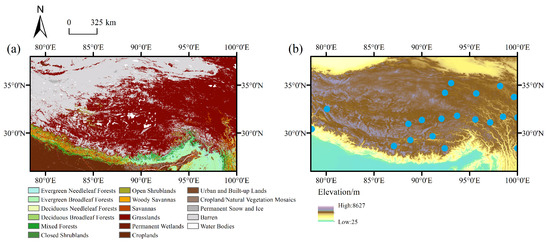
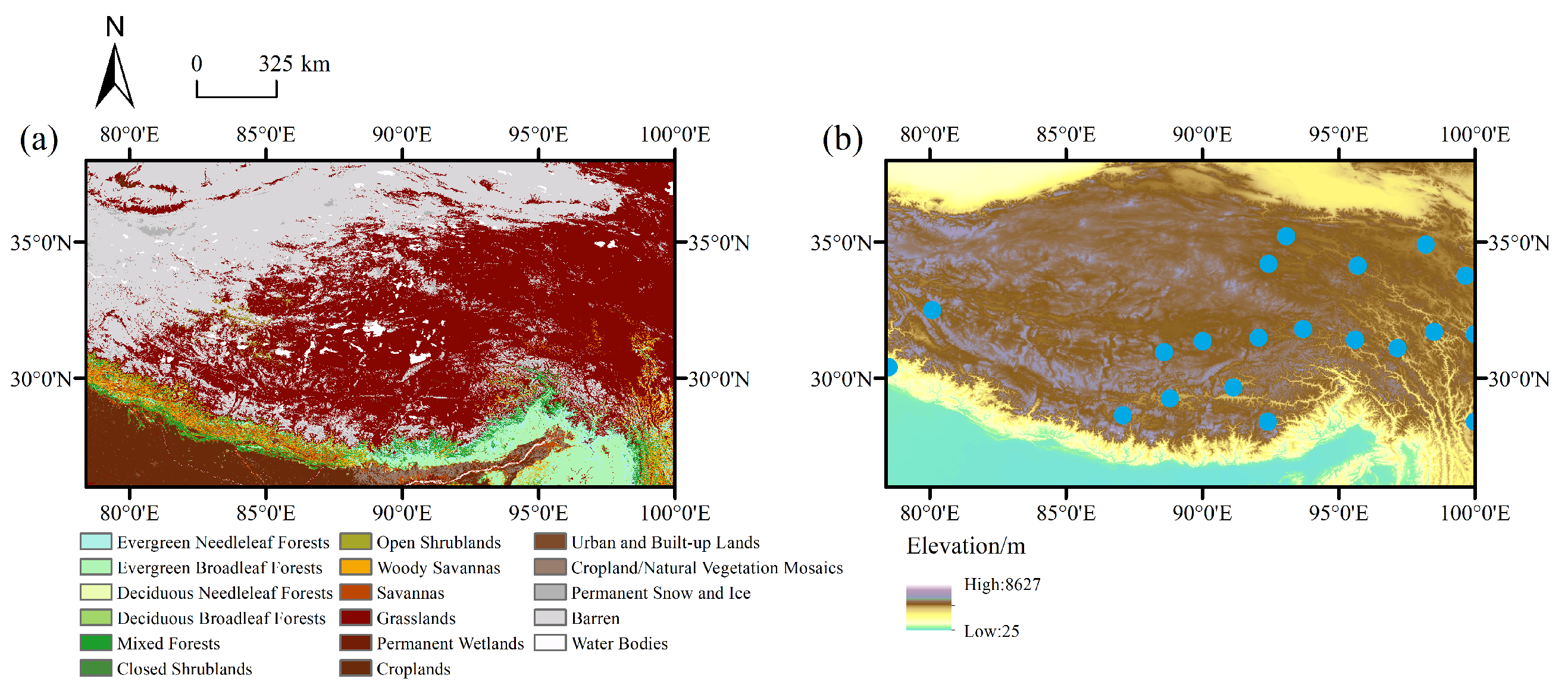
The research area is located on the Tibetan Plateau in southwestern China, between latitudes 26°N and 38°N and longitudes 78°E and 100°E. An overview of the research area is presented in Figure 1. The distribution of land cover types is shown in Figure 1a. The primary land cover types consist of forests, grasslands, and agricultural areas. Coniferous forests and mixed forests dominate in the northeastern and northwestern regions, while vast grasslands are mainly distributed along the edges of the Qinghai-Tibet Plateau. The elevation distribution of the region is presented in Figure 1b. The terrain is complex and variable, displaying diverse landforms such as hills, mountains, and plateaus. The eastern region is primarily composed of plains and hills, with relatively flat topography. The southern edge is dominated by the Himalayan Mountain range and its glaciers. As the area approaches the boundary of the Tibetan Plateau, the terrain gradually rises, forming typical plateau and mountainous landforms.

Figure 1. Overview of the research area. (a) Land cover types in the research area. (b) Elevation of the research area.The locations of the stations from the National Climatic Data Center (NCDC) are marked with blue dots.

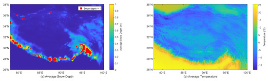
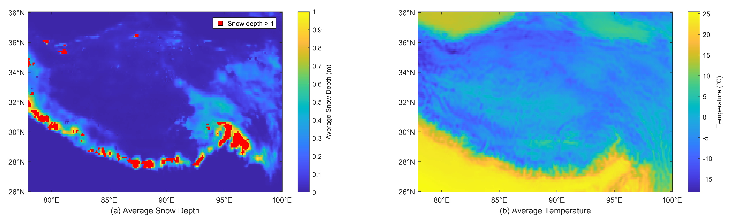
The annual average snow depth and temperature of the research area are shown in Figure 2. The snow depth distribution varies significantly, with areas where the annual average snowfall exceeds 1 m being marked in red in this study. These areas are typically located in the Himalayas, where the average snow depth reaches 9 m. However, in the central plateau, the annual average snow depth is generally shallower (less than 1 m). The average temperature of the region is shown in Figure 2b. Due to the influence of complex terrain, the average temperature exhibits significant spatial heterogeneity, with the central Tibetan Plateau experiencing a harsh climate, in which the average temperature remains below 0 °C, while the southern edge at lower elevations experiences higher average temperatures. The region has a subarctic and boreal climate, with the cold season typically lasting from late October to mid-April. The distinctive cold-temperate climate and intricate topography offer optimal conditions for investigating CYGNSS reflectivity reconstruction and F/T retrieval.

Figure 2. The annual average snow depth and average snow temperature of the study area: (a) Annual average snow depth. (b) Annual average temperature.

2.2. CYGNSS Datasets

The CYGNSS observation data from NASA is utilized in this research [38]. CYGNSS consists of eight microsatellites, which are specifically designed to measure tropical cyclone wind speeds and sea surface heights by reflecting GPS signals. These satellites were launched in 2016, with an orbital inclination of 35°. The spatial coverage of the constellation spans from approximately 38S to 38N. In terms of spectral characteristics, CYGNSS receivers operate in the L-band, capturing reflected Global Positioning System (GPS) L1 signals at a frequency of 1575.42 MHz. The temporal resolution is 7 h, and the spatial resolution is 7.0 × 0.5 km (upgraded to 3.5 × 0.5 km from July 2019). This research utilizes CYGNSS L1 Version 2.1 data, which covers the entire year of 2020. The reflected signals are recorded by the Delay-Doppler Map (DDM) of CYGNSS, which contains both coherent and incoherent components [39]. In this research, surface scattering is assumed to be primarily dominated by the coherent component, while incoherent reflections are disregarded [40]. Therefore, the CYGNSS reflectivity can be computed using the bistatic radar equation [41]. The specific equation is as follows:

$$\begin{array}{ccc}\hfill P_r& =& {\displaystyle \frac{P_t{G}_t}{4\pi {(R_{ts}+R_{sr})}^2}}{\displaystyle \frac{{{\lambda }_t}^2{G}_r}{4\pi }}{\mathrm{\Gamma }}_s\hfill \end{array}$$

(1)

where $P_r$ is the DDM peak power, $P_t$ is the transmit power. $G_t$ is the transmit antenna gain, $G_r$ is the receive antenna gain. $R_{ts}$ is the distance from the transmitter to the specular reflection point. $R_{sr}$ is the distance from the receiver to the specular reflection point. The effective surface reflectivity is represented by ${\mathrm{\Gamma }}_s$. ${\lambda }_s$ t denotes the wavelength of the GPS L1 signal. The value of ${\mathrm{\Gamma }}_s$ in decibels (dB) can be derived from the following equation:

$$\begin{array}{ccc}\hfill {\mathrm{\Gamma }}_s& =& 10\log P_r+20log(R_{ts}+R_{sr})+20log4\pi \hfill \\ & & -10log{P}_t-10\log G_t-10\log G_r-20\log {\lambda }_t\hfill \end{array}$$

(2)

2.3. SMAP Datasets

SMAP is an Earth observation satellite launched by NASA in 2015, which is designed to monitor soil moisture and soil F/T states [42]. Currently, SMAP completes global observations every 2–3 days. The SMAP L3 Global Daily EASE-Grid F/T product is used in this study as the evaluation and training dataset. In addition, SMAP also provides other surface observations, such as vegetation opacity and surface roughness. The datasets used in this research, including CYGNSS, SMAP, and auxiliary data, consistently span the period from January to December 2020.

2.4. Auxiliary Data

The accuracy of F/T retrieval is susceptible to various geophysical characteristics, including vegetation type and density, as well as surface water bodies. Therefore, the following auxiliary datasets are chosen as secondary features for the model: (1) Reflectivity, (2) Vegetation Water Content (VWC), (3) Roughness. The Reflectivity is derived directly from the CYGNSS L1 data. The Land Cover Type is extracted from the Moderate Resolution Imaging Spectroradiometer (MODIS) product (MCD12Q1) at a spatial resolution of 500 [43]. The International Geosphere-Biosphere Programme (IGBP) classification scheme, which defines 17 categories of land cover. Roughness is a necessary correction factor for microwave scattering models, influencing the transition between coherent and incoherent scattering. The Roughness parameter is obtained from the SMAP auxiliary product, representing the height variation of the soil surface. VWC is also extracted from SMAP auxiliary products to quantify the water mass in the vegetation canopy. The Topography data, represented by the Digital Elevation Model (DEM) from the Copernicus product (ESA) at a 90 m spatial resolution (https://doi.org/10.5270/ESA-c5d3d65), provides the elevation information. All auxiliary datasets are resampled both spatially and temporally to a unified scale and mapped to the EASE grid [44].

Additionally, soil temperature data from the European Centre for Medium-Range Weather Forecasts Reanalysis v5 (ERA5, with a spatial resolution of $0.{25}^{\circ }\times 0.{25}^{\circ }$ and an hourly temporal resolution) is utilized in this research to validate the F/T retrieval results (10.24381/cds.adbb2d47). To validate the retrieval results, ground truth data from the National Climatic Data Center (NCDC) are used [45]. NCDC is affiliated with the National Oceanic and Atmospheric Administration (NOAA), which integrates a variety of meteorological parameters. The 21 NCDC stations in the research area are selected for ground truth validation.

2.5. Quality Control

Quality control is crucial for ensuring data accuracy. The CYGNSS dataset includes quality flags, such as the power-on status of the S-band transmitter, blackbody DDM events, and satellite attitude errors. In accordance with CYGNSS’s official guidelines, data associated with specific quality flags are excluded. Reflections with peak power exceeding the boundaries of the 5–11 arrays or a Signal-to-Noise Ratio (SNR) below 2 dB are filtered out. Observations with a receiving antenna gain below 0 dB or an incidence angle greater than 65° are also discarded [46]. Finally, specular reflection points located in urban areas or over water bodies are excluded from the analysis.

3. Methodology

3.1. Reflectivity Reconstruction Model

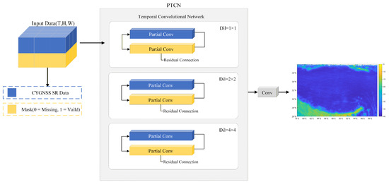
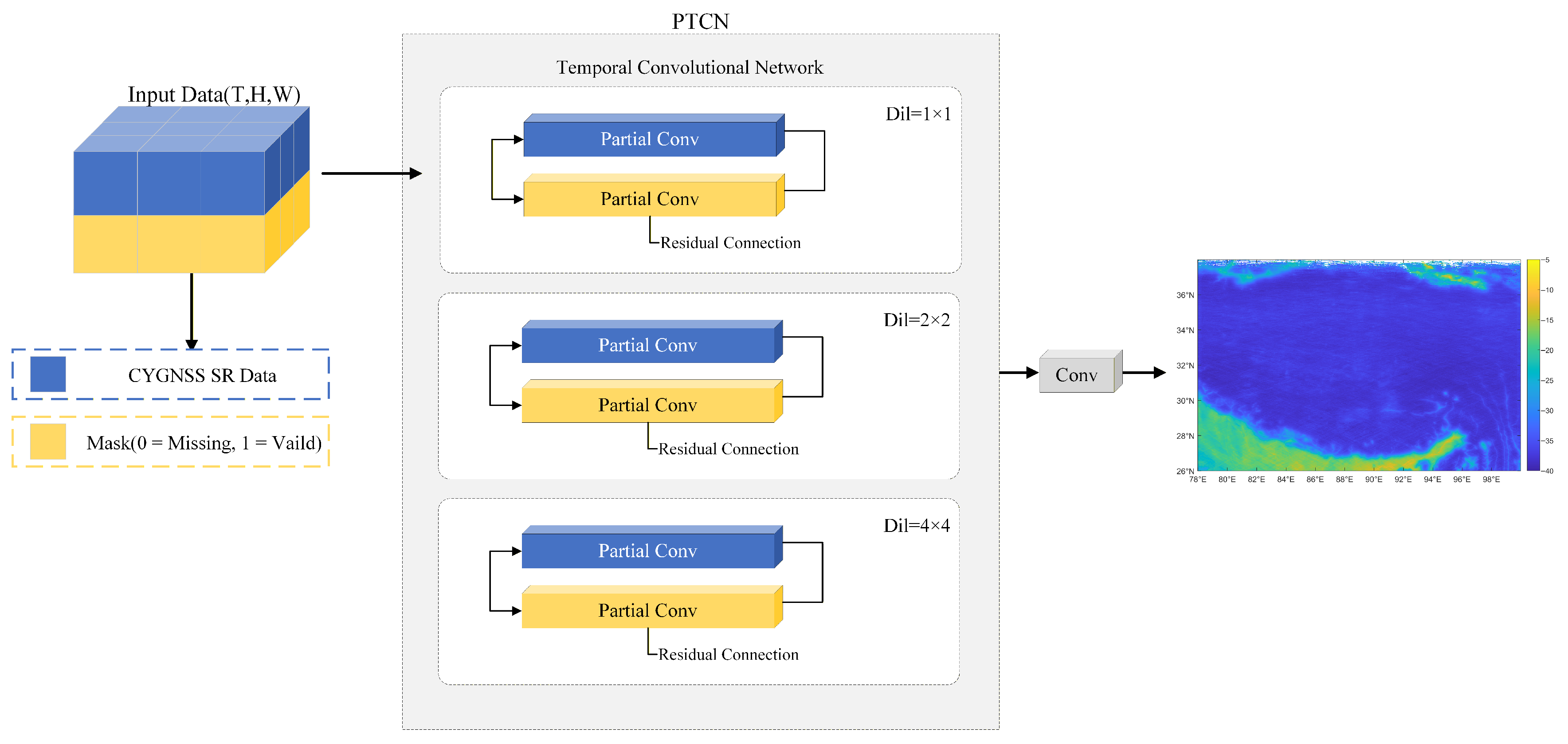
The overall architecture of the model is shown in Figure 3. It consists of a biased convolutional and a temporal convolutional network. The partial convolutional layer performs convolution operations on the input data and mask, which updates the mask accordingly. The partial convolution extracts features in the valid regions, while the missing regions are handled by the mask. The temporal convolutional network progressively extracts the spatio-temporal features from the time-series data, ultimately generating the reconstructed reflectivity.

Figure 3. Architecture of the PTCN model.

The input to the model consists of two parts: the CYGNSS reflectivity values and the validity mask. Let the input image be $X\in {\mathbb{R}}^{T\times H\times W\times C}$, where $M\in {\mathbb{R}}^{T\times H\times W\times C}$ represents the validity mask (with valid values as 1 and missing values as 0). H and W denote the width and height of the image. C is the number of channels and T is the number of time steps. The partial convolution layer processes the input through the following steps:

$$\begin{array}{c}\hfill Y^{\prime }=Conv\left(X_{masked}\right)\ast M^{\prime }\ast \alpha \end{array}$$

(3)

∗ denotes element-wise multiplication. $X_{\mathrm{masked}}$ is the result of the element-wise multiplication of the input data X and the mask M, which ensures that only valid data is involved in the convolution operation. $M^{\prime }$ is the updated mask, which represents the positions of valid values. To prevent the mask from affecting the convolution results, a scaling factor $\alpha$ is introduced. The number of valid values within each local region is normalized. The calculation of this factor is as follows:

$$\begin{array}{c}\hfill \alpha ={\displaystyle \frac{kernel\_size}{\sum M}}\end{array}$$

(4)

$kernel\_size$ is the total number of pixels covered by the convolutional kernel, and $\sum M$ denotes the number of valid pixels within the current window.

After the convolution operation, the output result $Y^{\prime }$ is processed by the Temporal Convolutional Network (TCN). The TCN processes the input data layer by layer through multiple Temporal Residual Blocks. Each Temporal Residual Block includes a dilated convolution operation and a residual connection. The detail is as follows:

$$\begin{array}{c}\hfill Z_k={Conv}_{dilated}(Z_{k-1},{\theta }_k),k=1\dots K\end{array}$$

(5)

where ${\mathrm{Conv}}_{\mathrm{dilated}}$ denotes the dilated convolution operation. ${\theta }_k$ represents the convolution weights at the k-th layer. Dilated convolution enlarges the receptive field by introducing a dilation factor, thereby capturing dependencies at longer time scales. To prevent information from gradually vanishing through multiple layers, a residual connection is introduced:

$$\begin{array}{c}\hfill Z_k^{\prime }=Z_k+Z_{k-1},k=1\dots K\end{array}$$

(6)

The output $Z_k$ of each layer is added to the input $Z_{k-1}$ of the previous layer. The resulting output is denoted as $Z_k^{\prime }$. Finally, the residual output $Z_k^{\prime }$ passes through a convolutional layer to generate the final prediction $Y_{\mathrm{final}}$:

$$\begin{array}{c}\hfill Y_{final}=Conv\left(Z_k^{\prime }\right)\end{array}$$

(7)

3.2. F/T Retrieval Algorithm

Extreme Gradient Boosting (XGBoost) is employed in this study for F/T retrieval. XGBoost is an efficient implementation of Gradient Boosting Trees (GBT), which optimizes the loss function by constructing decision trees [47,48,49]. Unlike traditional single decision trees, each tree in XGBoost improves the model’s prediction performance by minimizing these residuals. In classification problems, the output of each tree is subjected to a weighted vote to obtain the predicted label. The advantage of XGBoost lies in its ability to capture complex nonlinear relationships between data features through the tree structure. The detail is as follows:

$$\begin{array}{c}\hfill FT=XGB(SR,ROU,VWC)\end{array}$$

(8)

SR represents the daily grid reflectivity of CYGNSS. ROU and VWC are the roughness coefficient and vegetation water content, respectively. The SMAP F/T product is utilized as the target variable.

3.3. Training Process

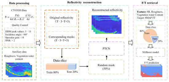
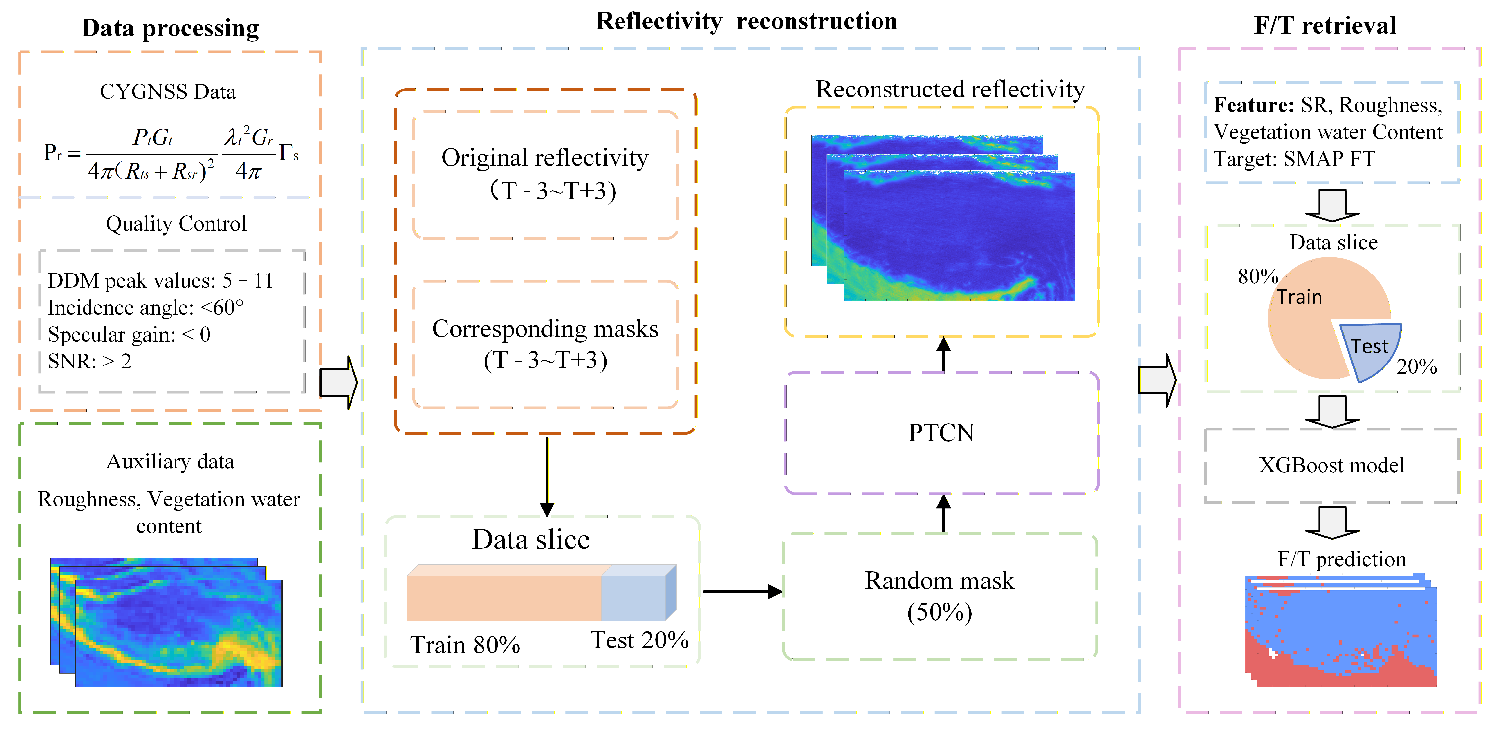
Figure 4 illustrates the specific process ranging from reflectivity reconstruction to the establishment of the F/T model. The datasets utilized for both reflectivity reconstruction and F/T modeling span the entire year of 2020. Following quality control, all data is applied to the reconstruction and F/T retrieval tasks. In this research, the CYGNSS reflectivity is applied with a mask. Masks and reflectivity together constitute the data required for reconstruction, which is divided into training and testing sets at a ratio of 8:2. During the construction of the training set, 50% of the original reflectivity is randomly removed to simulate missing data input into the model. Longer time windows lead to a lack of data timeliness, while shorter time windows result in lower coverage. Therefore, a preliminary experiment on the time window length is conducted in this research, which is shown in Table A2. The 1-day window is found to have sparse spatial coverage (25.6%). The 5-day time window, which extends the time span, results in a slight increase in coverage (65.7%) while retrieval accuracy decreases. In addition, the 5-day time window indicates that CYGNSS observations from beyond the current week are used for reconstruction, which typically smooths the temporal characteristics of the reflectivity. Therefore, the time window size in this study is set to three days before and after the target day. Specifically, the training data includes the reflectivity data from three days before and after the target center day T (i.e., T − 3 to T + 3). The data input to the model consists of the partially removed reflectivity and its corresponding mask. Additionally, the Adam optimizer is used. The trained model is applied to reconstruct reflectivity, effectively filling the gaps within the reflectivity dataset. Subsequently, this reconstructed dataset is utilized for F/T retrieval. The dataset for F/T retrieval comprises the roughness coefficient, vegetation water content, and the reconstructed reflectivity. This dataset is randomly partitioned into training and testing sets at an 8:2 ratio. Finally, the results are output by the XGBoost model.

Figure 4. Flowchart of the proposed soil freeze/thaw retrieval framework based on CYGNSS reflectivity reconstruction. In the F/T prediction map, the red area represents thawed, and the blue area represents frozen.

4. Results and Discussion

4.1. Reflectivity Reconstruction Results

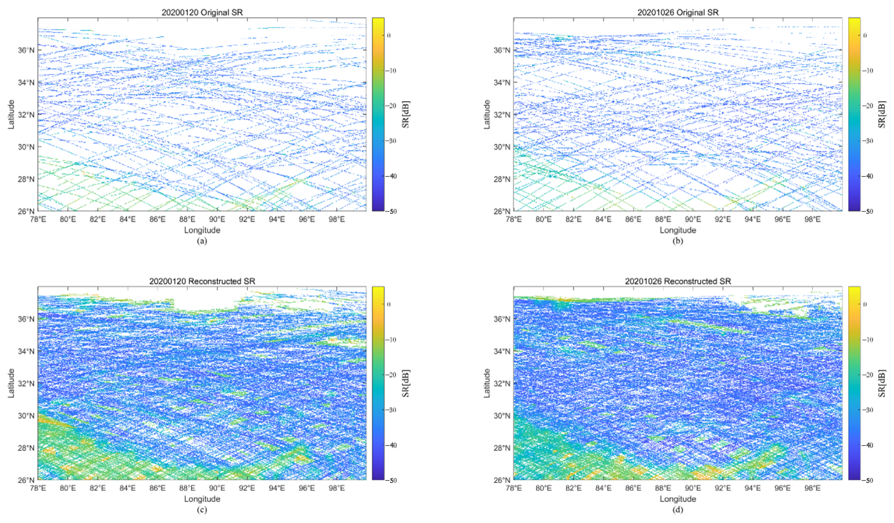
The original reflectivity and the reconstructed reflectivity datasets are compared in both spatial and temporal aspects. The reflectivity before and after reconstruction on January 20 and October 26 is shown in Figure 5. Figure 5c,d demonstrate that the missing values of reflectivity in high-altitude regions can be reconstructed by the PTCN model. Reflectivity is highest around the Himalayas, while it is relatively low in the interior of the Tibetan Plateau.

Figure 5. Examples of reflectivity distribution before and after reconstruction. (a,c) show the spatial distribution of reflectivity before and after reconstruction on 20 January 2020, respectively. (b,d) display the spatial distribution of reflectivity before and after reconstruction on 26 October 2020.

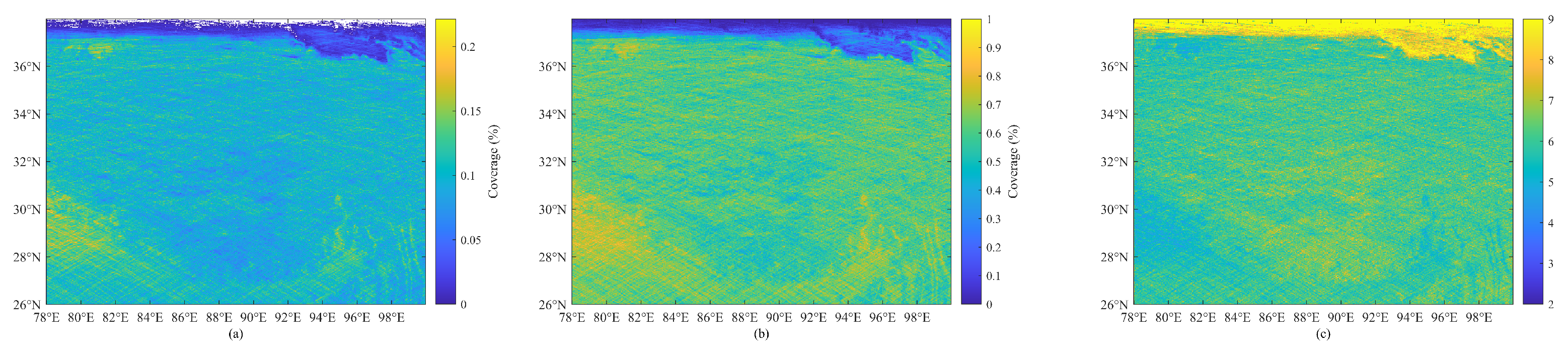
A comparative analysis of the coverage before and after reconstruction is shown in Figure 6. The coverage is calculated by dividing the number of valid observations for the grid by the total number of days in the year. The original coverage in the region is highest at 20%, while the reconstructed reflectivity achieves a maximum coverage of approximately 90%. The overall average coverage before and after reconstruction is computed, with the reconstructed coverage being six times that of the original observation data. The lower coverage of CYGNSS observation data above 37°N is due to the limitations imposed by the satellite’s orbit inclination. In contrast, the reconstructed coverage in areas south of 37°N reaches over 65%.

Figure 6. Reflectance coverage before and after reconstruction. (a) Coverage before reconstruction. (b) Coverage after reconstruction. (c) Coverage ratio before and after reconstruction.

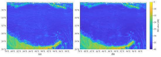
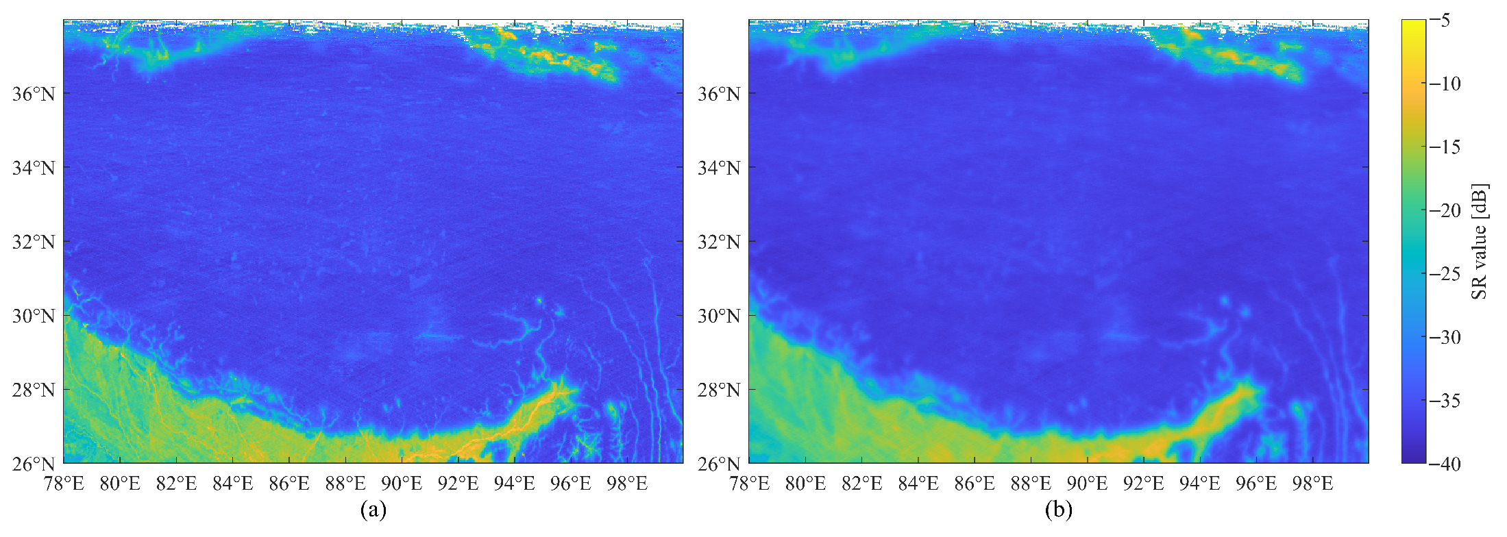
The overall distribution of reflectivity before and after reconstruction is shown in Figure 7. It can be observed that the distribution in Figure 7a before reconstruction and Figure 7b after reconstruction is relatively consistent. Reflectivity is lower in the interior of the Tibetan Plateau, while it is higher in the peripheral regions. Additionally, the mountainous areas along the Himalayas and the southeast exhibit smoothing effects. This is primarily due to the complex terrain and high surface roughness in these regions, which leads to sparse original CYGNSS observations and severe incoherent scattering. Combined with the effect of the time window, the model shows smoother results in these areas.

Figure 7. Average distribution of reflectance before and after reconstruction. (a) Average reflectance before reconstruction. (b) Average reflectance after reconstruction.

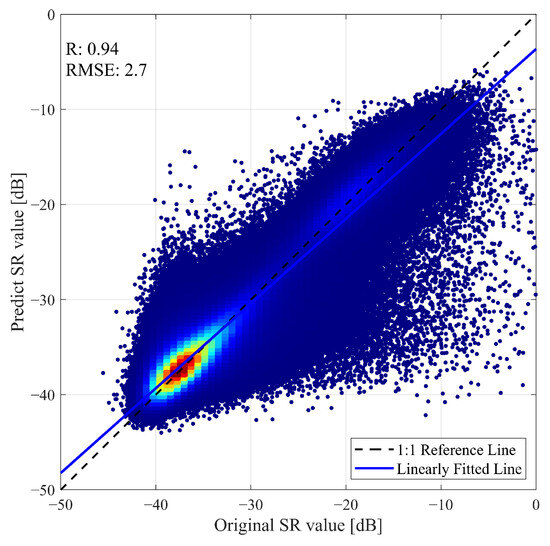
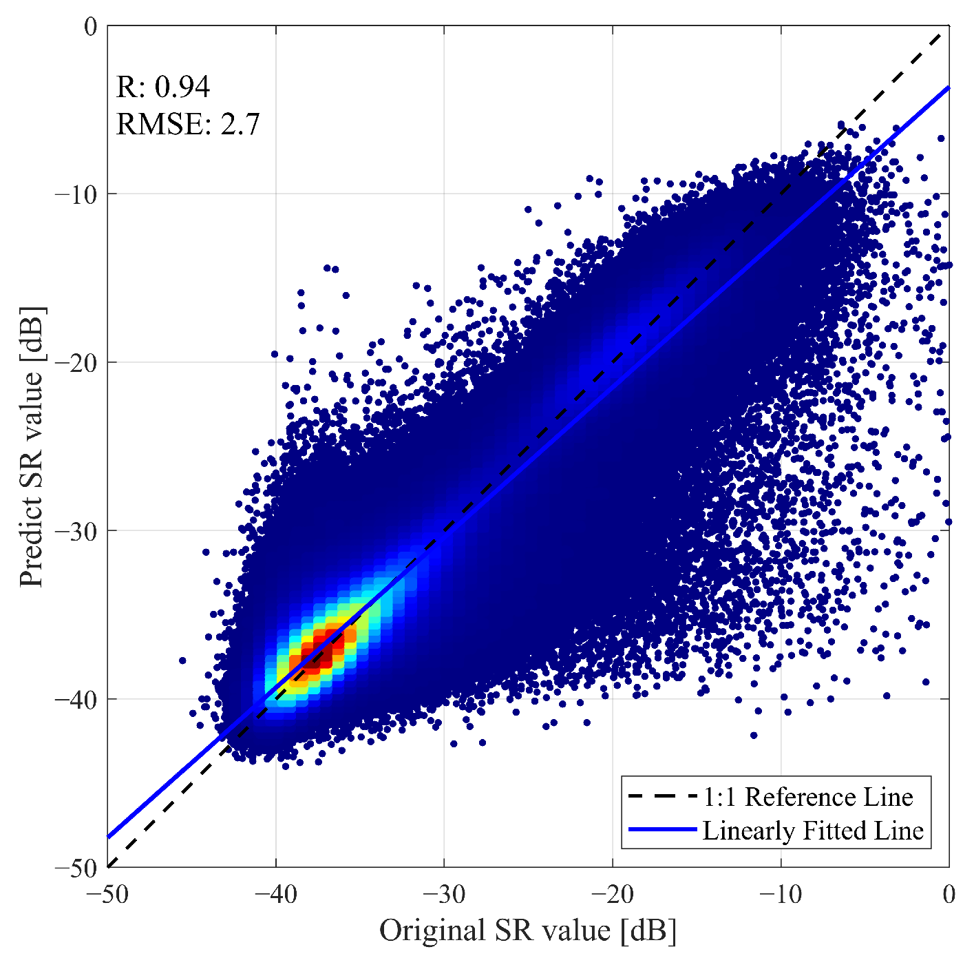
This research is the first to quantitatively evaluate the reconstructed reflectivity by simulating missing values, which uses R and RMSE to assess the model’s reconstruction performance. The scatter plot of the model’s reconstructed values versus the original values for the simulated missing observations is shown in Figure 8. The value of R reaches 0.92 (p < 0.001), and the value of RMSE reaches 2.7 dB.

Figure 8. Scatter plot of the predicted reflectivity from the proposed model (y-axis) versus the original CYGNSS reflectivity (x-axis). The solid line represents the 1:1 reference line.

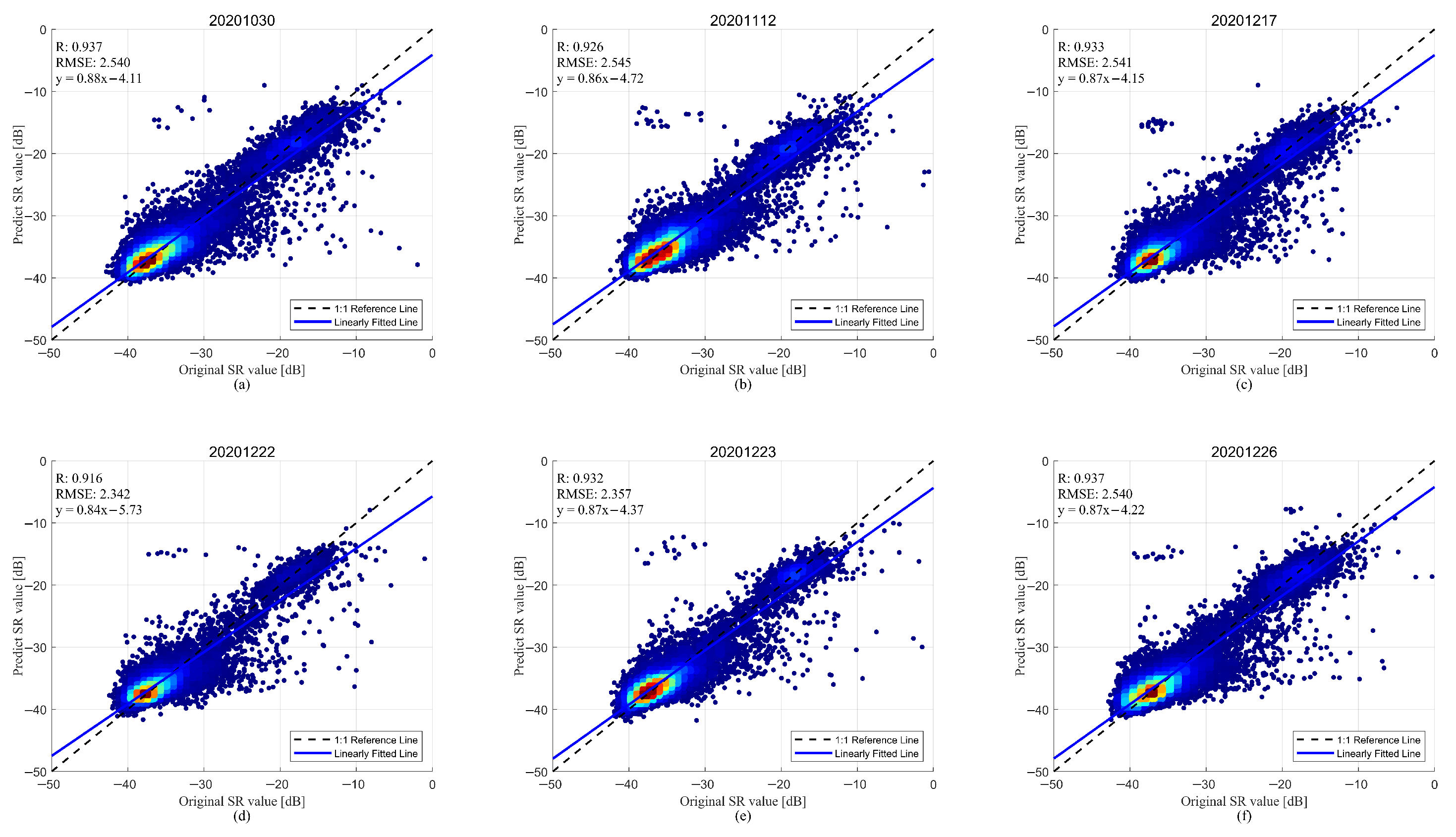
On the temporal dimension, the reconstructed reflectivity is compared with the original reflectivity at the daily scale. The scatter plots of the original and reconstructed reflectivity for different dates are shown in Figure 9. On 30 October, the value of R reaches 0.937 (p < 0.001) and the value of RMSE reaches 2.54 dB. On 17 December, the value of R reaches 0.933 (p < 0.001) and the value of RMSE reaches 2.541 dB. The best performance is achieved on 22 December. The value of R reaches 0.916 (p < 0.001) and the value of RMSE reaches 2.342 dB. These results indicate that the PTCN reconstruction model successfully fills the missing values in the original reflectivity data, which enhances its spatial coverage.

Figure 9. Scatter plots of observed versus predicted reflectivity across different dates. The subplots correspond to the results for (a) 30 October 2020, (b) 12 November 2020, (c) 17 December 2020, (d) 22 December 2020, (e) 23 December 2020, and (f) 26 December 2020.

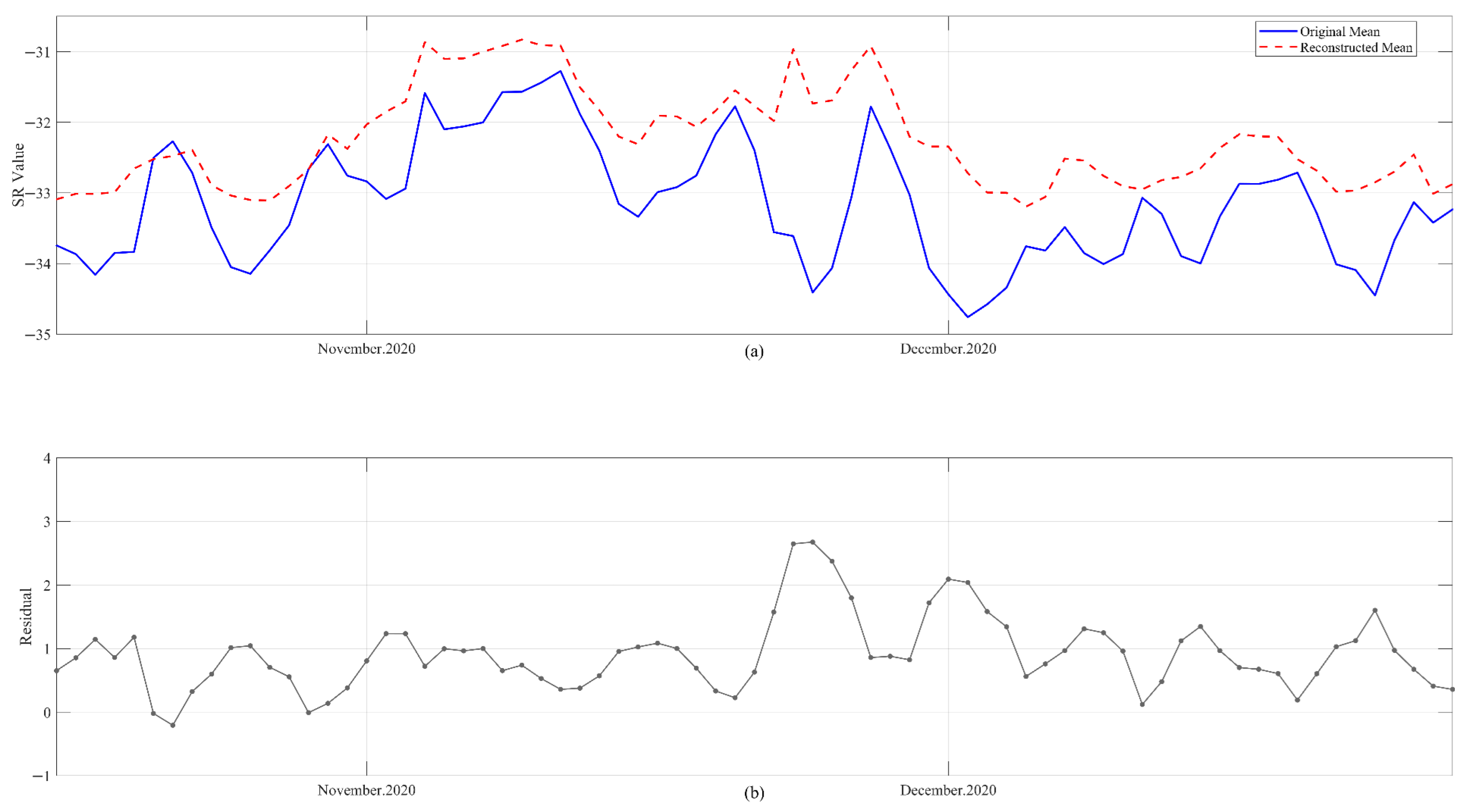
To further evaluate the model’s performance on the time series, the daily average reflectivity is calculated. The daily average reflectivity before and after reconstruction from 17 October to 27 December is shown in Figure 10. It can be observed that the reconstructed reflectivity closely follows the trend of the original values. The daily residuals before and after reconstruction are shown in Figure 10b. At the daily scale, the average residuals before and after reconstruction range from 0 to 2.5.

Figure 10. Temporal variation of reflectance after reconstruction. (a) Day average reflectivity value. (b) Residuals before and after reconstruction.

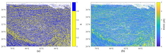
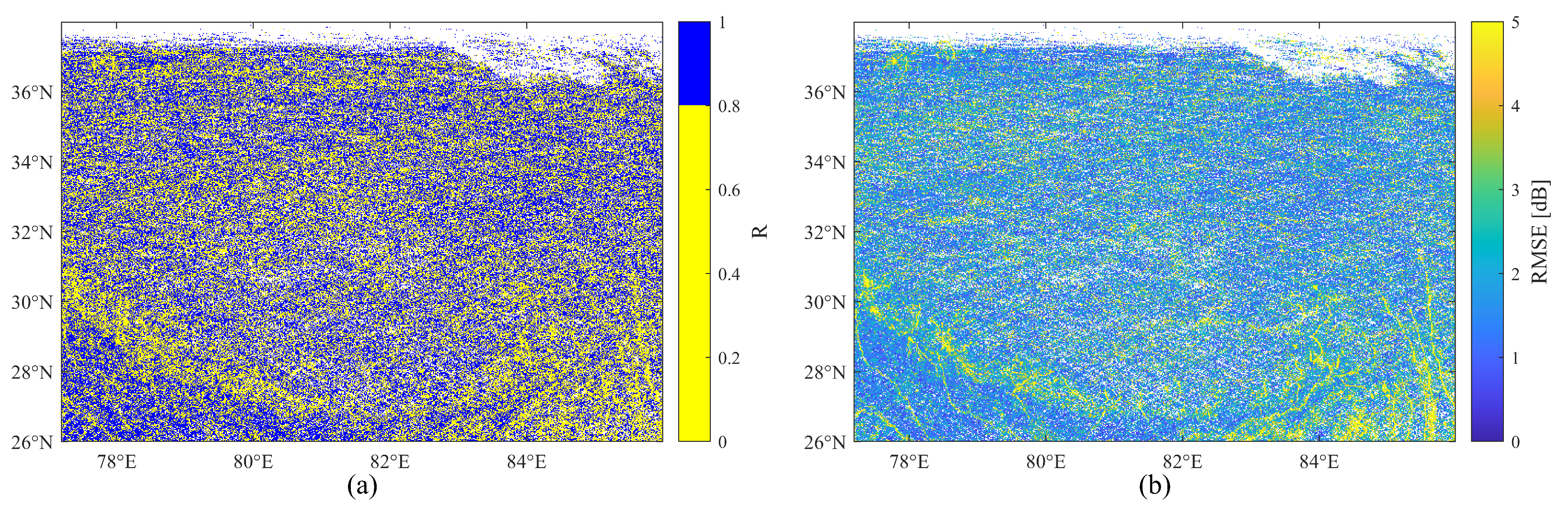
Moreover, the R and RMSE between the reconstructed and original reflectivity are calculated for each grid. Figure 11 shows the spatial distribution of these time statistics. As shown in Figure 11a, the value of R is above 0.8 in the vast majority of the study area. Figure 11b indicates that the RMSE value is around 2dB in most regions. Furthermore, the areas with relatively low reconstruction performance are mainly concentrated along the edge of the Himalayas and in the southeastern part of the study area. This localized performance degradation is primarily attributed to the extremely high altitude and large surface roughness in these regions. The rugged and complex terrain induces strong incoherent scattering, which in turn affects the quality of the reflected signal. As a result, the model exhibits a decline in performance in these areas.

Figure 11. Performance distribution before and after reconstruction on the time series. (a) Correlation coefficient (R). (b) RMSE.

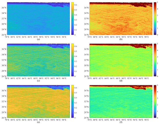
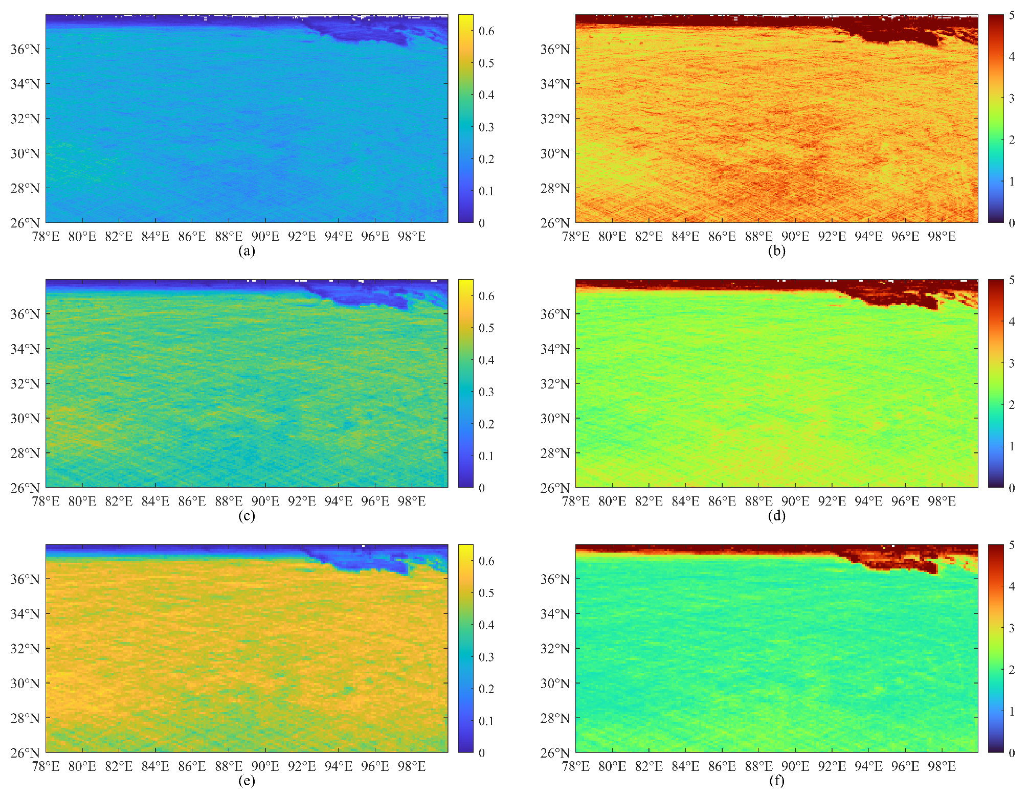
The performance is evaluated at coarser scales by aggregating the data to resolutions of 6, 9, 12, 18, and 36 km. The 9 km and 36 km resolutions are particularly important as they align with the standard resolutions adopted by current remote sensing products (e.g., SMAP). The variations in coverage before and after reconstruction at different spatial resolutions are analyzed in this research, which are shown in Figure 12. In the annual sequence of the study area, the original CYGNSS reflectivity is found to achieve peak coverage of 37.4%, 51.64%, and 64.21% at 6 km, 9 km, and 12 km, respectively. The average coverage is 23.5%, 36%, and 62.3%, respectively. The average reflectance coverage at 6, 9, and 12 km after reconstruction reaches 85.9%, 92.8%, and 94.5%, respectively.

Figure 12. Coverage before reconstruction and the relative improvement in coverage after reconstruction at different spatial resolutions. (a,c,e) Original coverage at 6 km, 9 km, and 12 km, respectively; (b,d,f) Ratio of coverage improvement after reconstruction relative to before reconstruction at corresponding spatial resolutions.

The reconstruction performance at different spatial resolutions is further evaluated in this research. The detailed statistical results are shown in Table 1. After reconstruction, the reflectivity coverage at 6, 9, and 12 km is obtained, which is found to be 3.9, 2.82, and 2.29 times the original, respectively. As the spatial resolution decreases from 6 km to 36 km, the data coverage progressively increases from 85.9% to 97.7%. At a resolution of 3 km, the coverage is 6 times that of the original data. At 36 km resolution, the reconstructed reflectivity is 1.3 times that of the pre-reconstruction reflectivity.

Table 1. Reconstructed reflectivity coverage at different spatial resolutions.

Spatial Resolution	Reconstructed Reflectivity Coverage (%)	Several Times That of the Original Observation (Times)	Time Window (Day)
3 km	60	6	3
6 km	85.9	3.8	3
9 km	92.8	2.82	3
9 km ([32])	87.8	2.78	10
12 km	94.5	2.28	3
18 km	96.1	1.77	3
36 km	97.7	1.3	3

Furthermore, a comparative analysis at 9 km resolution reveals that the proposed method outperforms the approach by [32] in terms of performance. This method achieves a coverage of 92.8% within a 3-day time window, without the use of any auxiliary data. This demonstrates that the method is capable of reducing the time window while maintaining a good spatial coverage and data reconstruction efficiency.

In conclusion, the reconstructed reflectivity dataset not only enhances spatial coverage but also captures the temporal variation of reflectivity. High spatio-temporal resolution reflectivity data can be indirectly used for F/T retrieval. Therefore, the F/T retrieval accuracy before and after reconstruction can also serve as a measure of the effectiveness of this method.

4.2. F/T Retrieval Results

4.2.1. Comparison with Different F/T Products

The F/T retrieval models before and after reconstruction compare their prediction results with the F/T product to assess accuracy. SMAP, as the primary validation data, defines its F/T state by combining the maximum reflectance ratio at the point of impact with the estimated effective soil temperature threshold. In this study, the F/T state of the ERA5 dataset is defined as follows: daily average soil temperature above 0 °C is considered thawed, and below 0 °C is considered frozen. To enable a more rigorous evaluation of the reconstructed F/T retrieval performance, F/T retrievals are implemented at spatial resolutions of 9 km and 36 km.

Table 2 presents the F/T retrieval performance before and after reconstruction at different spatial resolutions. Relative to SMAP, the F/T retrieval accuracy at 36 km before and after reconstruction are 90% and 91%, respectively. In most regions, the retrieval performance remains largely unchanged, indicating that the reconstructed F/T accuracy is comparable to that prior to reconstruction. At 9 km resolution, the corresponding accuracy reaches 83.6% and 85.4%. Compared with ERA5, the F/T retrieval accuracy at 36 km is 85.76% before reconstruction and 85.81% after reconstruction. At 9 km, the accuracy increases from 81.95% to 83.26% after reconstruction. Overall, the F/T retrieval accuracy before and after reconstruction are broadly consistent, indicating that the proposed reconstruction approach effectively captures soil F/T states in most cases.

Table 2. F/T retrieval performance before and after reconstruction at different spatial resolutions.

FT Accuracy (%)	Compared with ERA5 (%)		Compared with SMAP (%)
	Ori FT	Res FT	Ori FT	Res FT
36 km	85.76	85.81	90	91
9 km	81.95	83.26	83.6	85.4

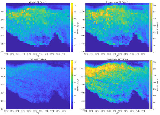
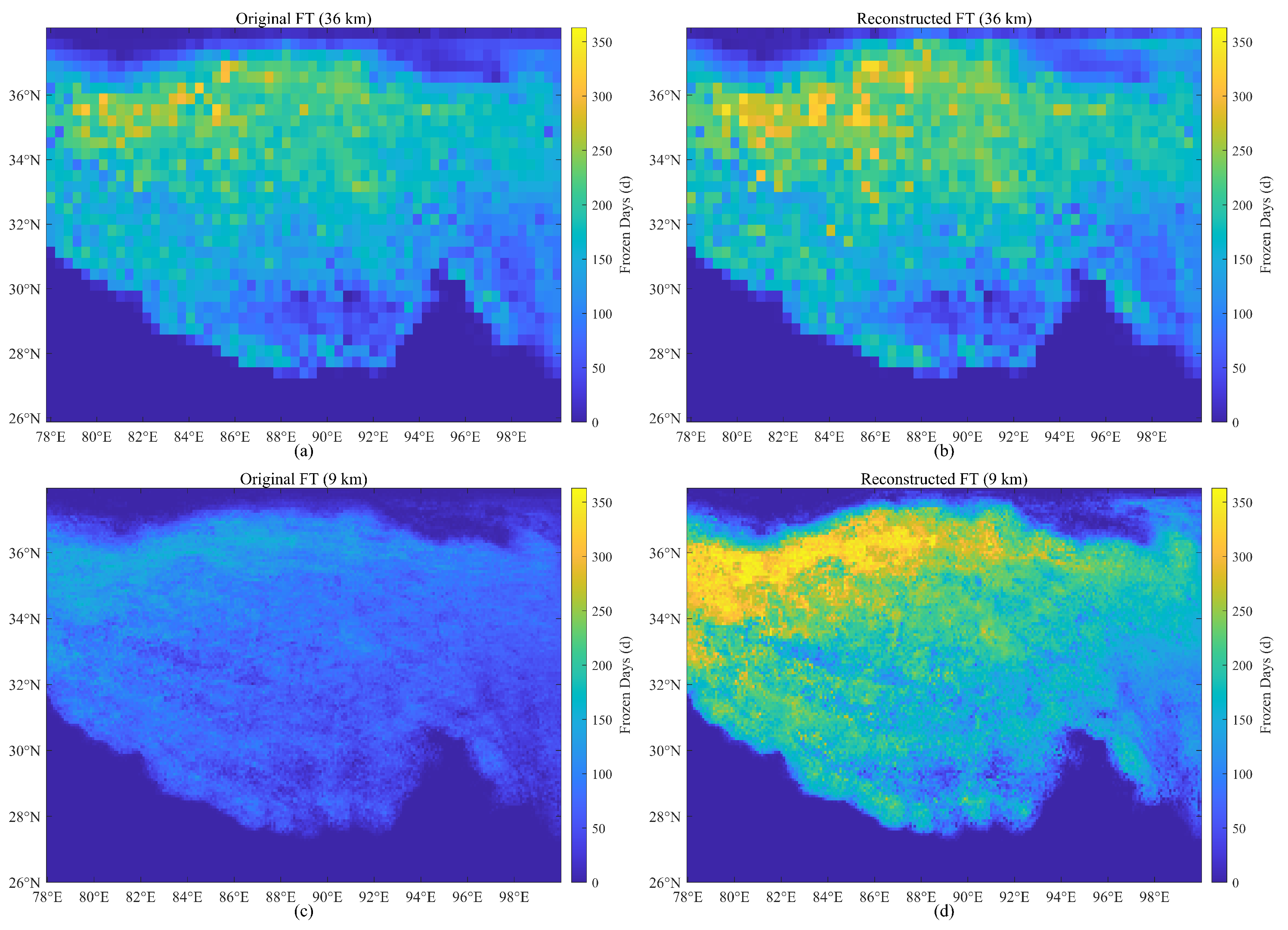
The frozen days within the available observation period before and after reconstruction at different spatial resolutions are shown in Figure 13. Figure 13a,b illustrate the number of frozen days at 36 km before and after reconstruction, respectively. Permafrost is predominantly distributed in the north-western Tibetan Plateau, whereas seasonal F/T variability mainly occurs in the central plateau. Figure 13c,d present the number of frozen days at 9 km before and after reconstruction. The difference in the number of frozen days before and after reconstruction at the 9 km resolution is primarily due to the sparse temporal coverage of the original 9 km resolution CYGNSS observation data. The difference in the number of frozen days before and after reconstruction at the 9 km resolution is primarily due to the sparse temporal coverage of the original 9 km resolution CYGNSS observation data. In this research, the calculation of frozen days is strictly based on the available valid observation days. The original CYGNSS F/T retrieval at 9 km resolution is notably sparse, with an average availability of only 132 days prior to reconstruction. Therefore, the statistics of cold days are limited by the finite number of effective observation days. In contrast, the reconstructed product effectively fills these temporal gaps. The spatial distribution pattern of the reconstructed frozen days remains consistent with that of the original data. It can be observed that the F/T distributions at 9 km and 36 km are broadly consistent throughout the effective observation period. Moreover, within their respective effective observation periods, the spatial distribution of frozen days before and after reconstruction at both 9 km and 36 km resolutions also shows consistency. The freezing duration in the north-eastern part of the plateau is longer than that in the central region. The south-eastern part of the plateau exhibits a relatively shorter freezing period, indicating more frequent F/T transitions.

Figure 13. Freezing days before and after reconstruction at different spatial resolutions. (a,b) Freezing days before and after reconstruction at 36 km resolution; (c,d) Freezing days after reconstruction at 9 km resolution.

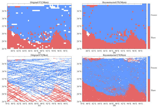
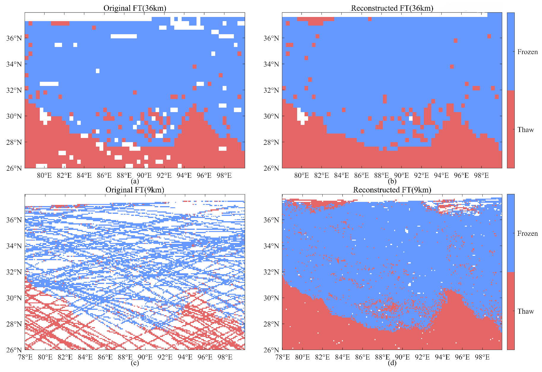
Figure 14 presents the F/T retrieval results before and after reconstruction at different spatial resolutions for 10 January 2020. The F/T distributions before and after reconstruction are largely consistent in their primary spatial patterns. On 10 January, the frozen surface is predominantly located in the central Tibetan Plateau, while thawed conditions prevail in the surrounding areas. CYGNSS observations are sparse near 37°N, which results in missing F/T values. At both 36 km and 9 km resolutions, the reconstructed F/T products fill the gaps present in the original observations. Notably, at 9 km resolution, Figure 14c,d indicate that the reconstruction method produces a more pronounced improvement at higher spatial resolution. Furthermore, this suggests that the method is more effective at filling the observational gaps in SMAP.

Figure 14. F/T retrieval distribution results before and after reconstruction. (a,b) FT retrieval results before and after reconstruction at 36 km resolution; (c,d) FT retrieval results before and after reconstruction at 9 km resolution.

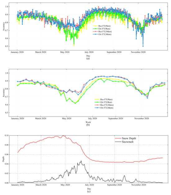
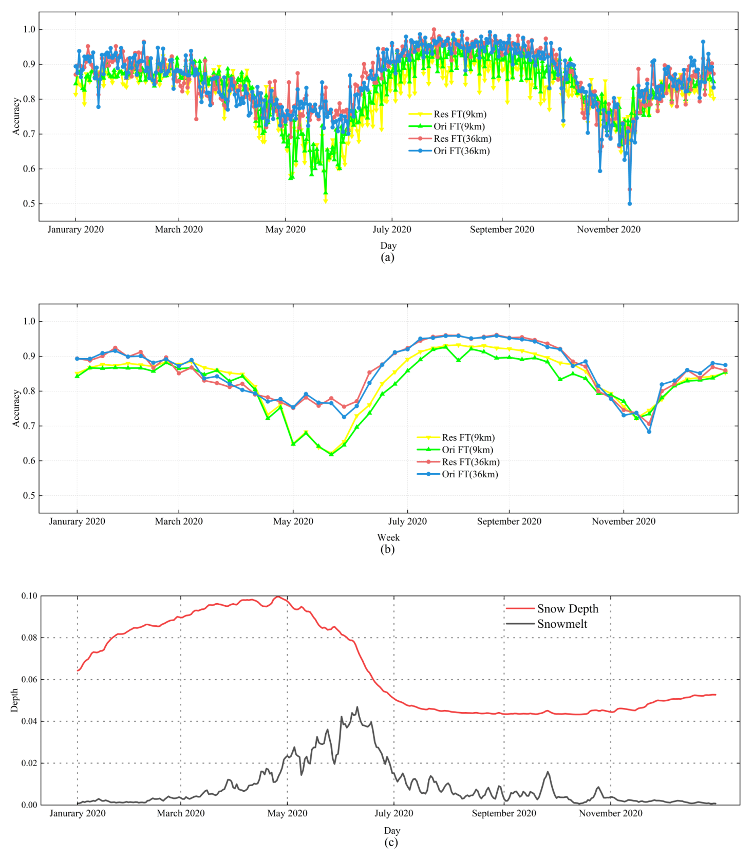
The F/T retrieval performance before and after reconstruction at weekly and daily scales is shown in Figure 15. The F/T retrieval accuracies after reconstruction at different spatial resolutions exhibit similar seasonal variation patterns. At the daily scale, the overall F/T accuracy at 36 km remains largely within the range of 0.8 to 0.95. At the weekly scale, the fluctuations become more stable, with accuracy generally exceeding 0.8. In contrast, the F/T variations at 9 km are more pronounced. This is attributed to stronger heterogeneity at higher spatial resolution, which makes the affected variations more pronounced. At 36 km resolution, the coarser scale attenuates the influence of seasonal variability.

Figure 15. ERA5 validation of F/T retrieval results before and after reconstruction at different time scales. (a) Daily scale. (b) Weekly scale. (c) Changes in Snow Depth and Snowmelt.

These two products exhibit higher stability and greater accuracy during the retrieval process in the summer months (July to September), while a decrease in retrieval accuracy is observed during the transitional seasons. The accuracy of F/T retrieval is influenced by snow coverage. This research analyzes the cause of performance degradation through changes in snow depth and snowmelt. The daily variations in snow depth and snowmelt are shown in Figure 15c. During the period from January to March, the diurnal temperature variation is small, snow depth is high, and snowmelt is limited. The higher snow depth affects the model’s performance, but the limited snowmelt indicates that the snow is primarily in a dry state during this period. As snow depth increases, the model’s performance begins to be impacted. During the spring transition season (April to June), snowmelt increases, reaching its peak in June. The increase in liquid water content significantly raises the dielectric constant of the snow, with the snow primarily in a wet state. The wet snow state results in higher reflectivity. Additionally, the larger diurnal temperature variation leads to more frequent freeze/thaw transitions. This leads to a decline in retrieval accuracy during this period, which is observed in the results. From July to September, the effects of snowmelt and snow depth decrease, and the model’s accuracy stabilizes. However, during the autumn transition season (October to November), the increase in diurnal temperature variation results in more frequent freeze/thaw transitions, which impacts the model’s performance. Meanwhile, snowmelt also exhibits significant fluctuations, which further contribute to the decline in performance. In December, snowmelt variations tend to cease, and freeze/thaw transitions weaken, which leads to an improvement in the model’s performance.

The change curves before and after reconstruction indicate consistency throughout the entire time series. This indicates that the reconstruction method used in this study preserves the original physical characteristics and accuracy trends while reconstructing the data.

4.2.2. Analysis of Retrieval Performance by Elevation and Land Cover Type

As a key geographical factor, elevation plays an important role in the retrieval accuracy. Therefore, this research analyzes the impact of different elevation levels on the retrieval accuracy.

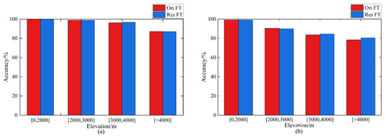
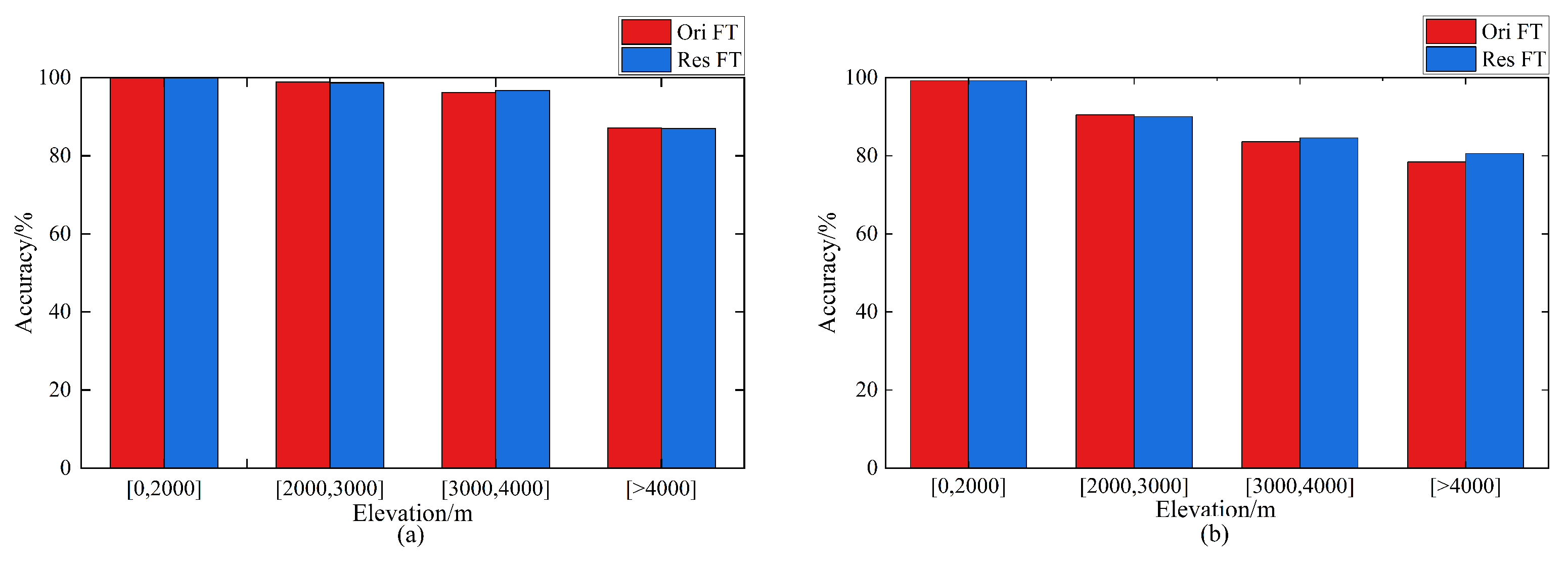
Figure 16 shows the FT retrieval performance before and after reconstruction at different elevation levels. Both demonstrate similar performance at different elevation levels. With the increase in elevation, the FT retrieval accuracy of both shows a decline. In regions below 3000 m elevation, the F/T accuracy at 36 km and 9 km reaches 96% and 84%, respectively. In high-altitude areas above 4000 m, the accuracy decreases to 86% and 80%.This is due to the significant diurnal temperature variation with increasing elevation, which affects the F/T transition process. The proposed method is unable to capture these frequent F/T transitions effectively.

Figure 16. F/T retrieval accuracy before and after reconstruction at different Elevation. (a) F/T retrieval performance before and after reconstruction at 36 km resolution for different elevations. (b) F/T retrieval performance before and after reconstruction at 9 km resolution for different elevations.

Additionally, different land cover types have varying effects on the reflection signals. Therefore, the model’s performance under the influence of different land cover types is analyzed.

Table 3 presents the F/T retrieval performance before and after reconstruction, which is compared with SMAP across different land cover types.The data shows that the performance before and after reconstruction is generally comparable. Both perform well in categories such as Cropland/Natural Vegetation Mosaics, Croplands, and Savannas. However, the performance in Snow and Ice is relatively poor. This is due to the region being predominantly covered by ice and snow. In this research, it is assumed that CYGNSS primarily observes land surfaces with coherent reflections, where smooth ice and snow layers have higher reflectivity. Based on this assumption, the model may misclassify snow-covered regions as melting areas during the training process. Due to the high reflectivity of smooth surfaces, the model might incorrectly predict frozen soil as thawed, leading to predictions that do not align with the actual surface state of the frozen soil. This may account for the poorer performance of the models in this type.

Table 3. Performance of F/T before and after reconstruction across different land cover types.

Land Cover Type	Original Acc (36 km) (%)	Reconstructed Acc (36 km) (%)	Original Acc (9 km) (%)	Reconstructed Acc (9 km) (%)
Evergreen Needleleaf Forests	93.43	92.96	87.43	87.35
Evergreen Broadleaf Forests	100	99.72	94.9	94.2
Mixed Forests	90.53	90.63	87.6	87.84
Woody Savannas	99.4	99.61	95.98	96.41
Savannas	99.6	100	94.84	93.24
Grasslands	86.23	86	80.09	84.24
Croplands	99.9	100	95.3	95.6
Cropland/Natural Veg Mosaics	100	100	95.13	95.04
Snow and Ice	70.8	71.38	64.15	63.44
Barren	86.2	87.6	81.45	80.86

4.2.3. Filling in SMAP Observations

CYGNSS consists of eight satellites and provides excellent spatio-temporal resolution. SMAP has a revisit cycle of 2–3 days, with daily gaps in observation data. Therefore, this research investigates the reconstruction of CYGNSS and its role in filling observation gaps in SMAP data.

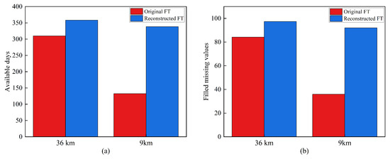
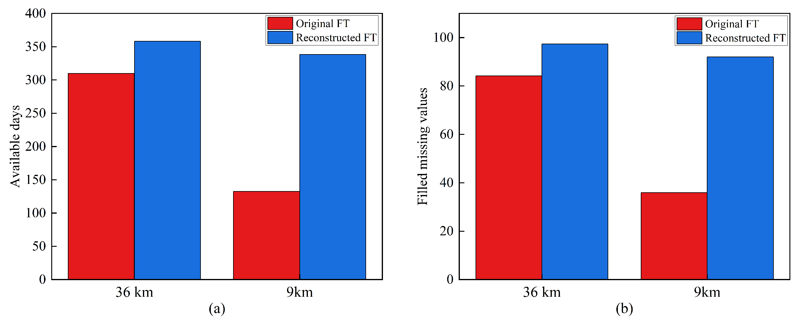
The number of effective observation days before and after reconstruction, as well as the spatial extent of observation gaps filled in SMAP, are shown in Figure 17. At 36 km resolution, the number of CYGNSS observation days before and after reconstruction is 310 and 358 days, respectively. After reconstruction, the number of observation days is 1.15 times that before reconstruction. At 9 km resolution, the number of observation days before and after reconstruction is 132 and 339 days, respectively. After reconstruction, the number of effective observation days is 2.56 times that of the original data. At 9 km resolution, the original F/T retrieval can fill 36% of the observational gaps in SMAP. After reconstruction, the F/T retrieval can fill 92% of these gaps. This indicates that the proposed reconstruction method effectively addresses the issue of temporal data gaps in observations. At the same time, this also highlights the trade-off between temporal and spatial resolution in CYGNSS observations.

Figure 17. Comparison of data availability before and after reconstruction at different spatial resolutions (36 km and 9 km). (a) Comparison of available days. (b) Comparison of filled missing values.

4.2.4. Ground Station Validation

Data from 21 NCDC stations are used to validate the F/T retrieval results, which are used to evaluate the performance of F/T retrieval.The FT retrieval results before and after reconstruction are averaged to a daily scale, aligning with the temporal resolution of the observed stations. Ease-Grid grids are used to match the grid locations of the NCDC observation stations based on their latitude and longitude. For daily mean soil temperature, temperatures above 0 °C are considered to indicate a thawed state, while temperatures below 0 °C are considered to indicate a frozen state.

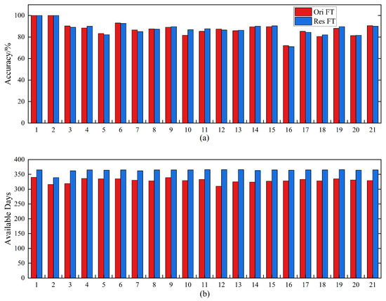
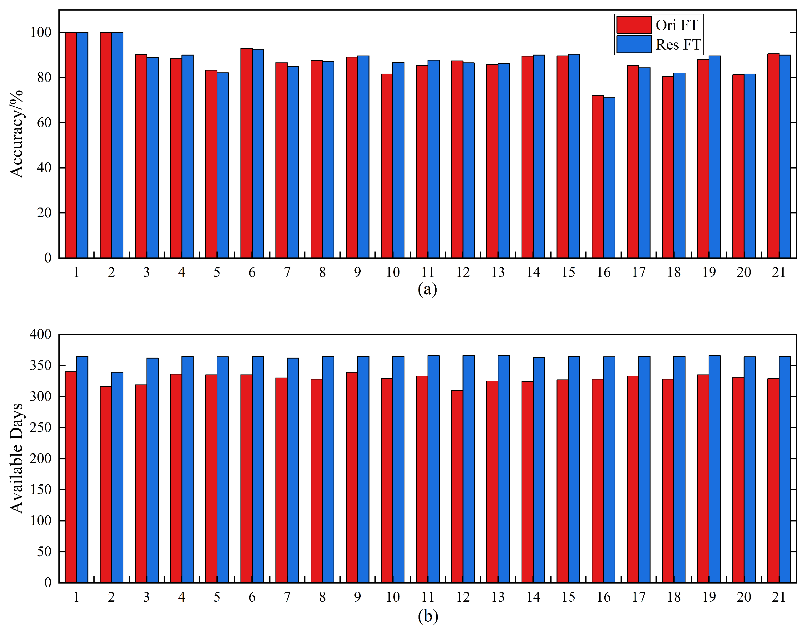
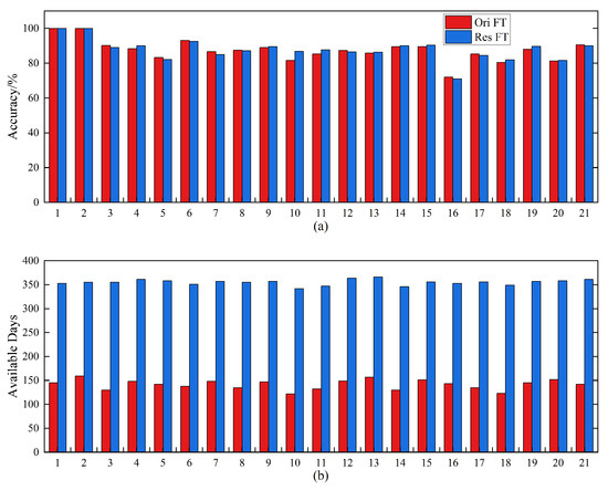
The F/T retrieval results at 36 km before and after reconstruction for the 21 stations are shown in Figure 18.

Figure 18. F/T retrieval accuracy and available days before and after reconstruction at 36 km resolution compared with ground stations. (a) F/T retrieval accuracy at different stations. (b) Available days at different stations.

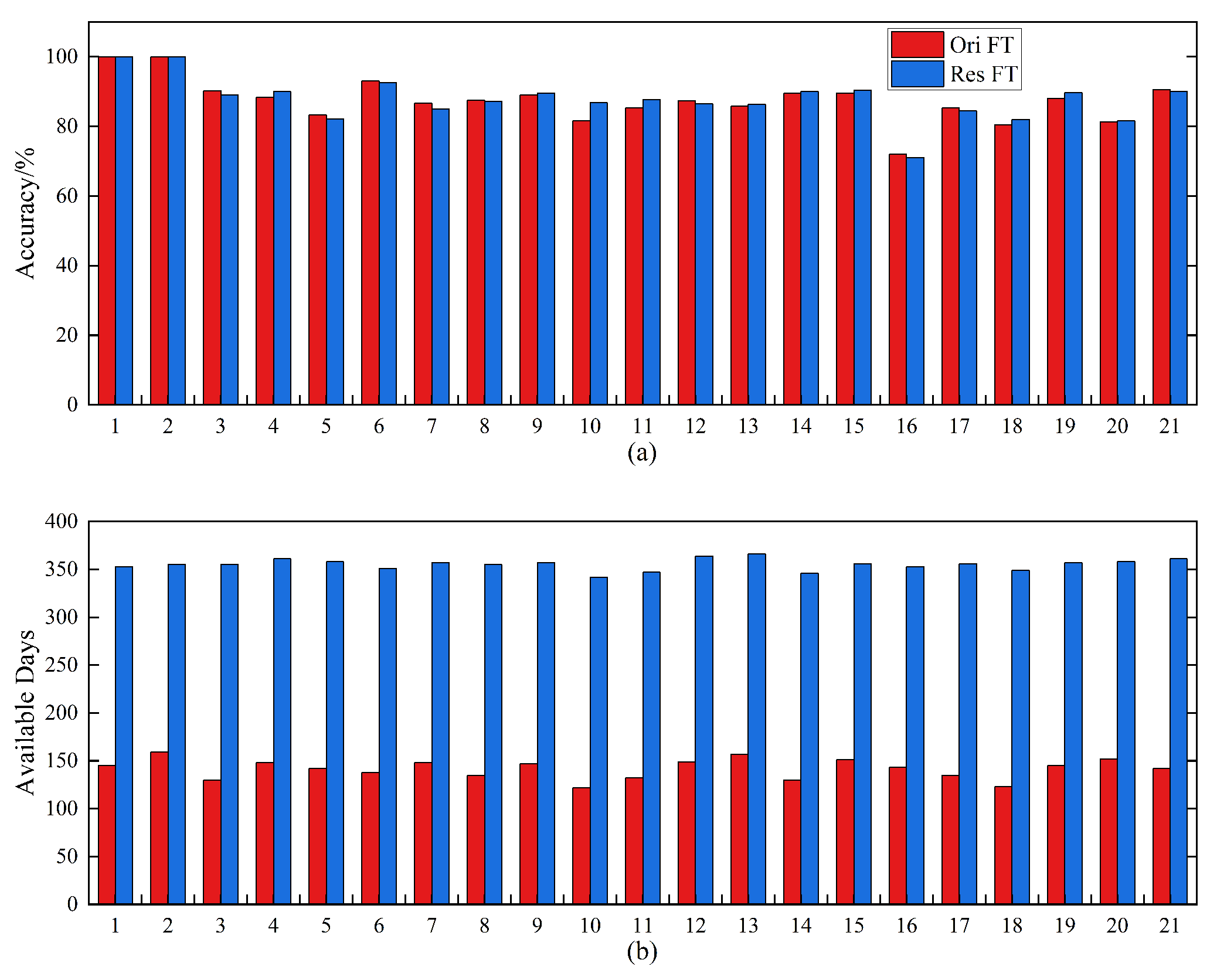
The 9 km F/T retrieval results before and after reconstruction for the 21 stations are shown in Figure 19. Additionally, Figure 19b presents the corresponding number of available observation days.

Figure 19. F/T retrieval accuracy and available days before and after reconstruction at 9 km resolution compared with ground stations. (a) F/T retrieval accuracy at different stations. (b) Available days at different stations.

Table A1 provides detailed statistics for all the observed stations. At 36 km resolution, the mean F/T retrieval accuracy across the stations reaches 87.38% before reconstruction and 87.71% after reconstruction, with similar performance observed at individual stations. At 9 km resolution, the mean accuracy is 83.9% before reconstruction and 82.3% after reconstruction. The reconstruction accuracy at 9 km resolution shows a slight decline, which is primarily attributed to the amplification of spatial heterogeneity and the characteristics of the SMAP 9 km data. Compared with lower-resolution data (such as 36 km), which smooths local variations, higher-resolution data (9 km) is more sensitive to the spatial heterogeneity of the surface. Additionally, the SMAP 9 km F/T product, which is used as the reference for validation, is obtained through the Backus-Gilbert spatial interpolation method. This interpolation process inherently introduces noise [50]. The mean number of available observation days after reconstruction increases by 256% compared with before reconstruction. The results demonstrate the effectiveness of the reconstruction method in enhancing temporal resolution, which is achieved while maintaining accuracy.

5. Discussion

To effectively evaluate the F/T retrieval performance in this research, Table 4 summarizes a comparison of F/T retrieval methods at different resolutions. This research implements F/T retrieval at 9 km and 36 km based on the reflectivity reconstruction algorithm. The average accuracy after reconstruction compared with the ground truth measurement stations is 87.71% at 36 km and 82.3% at 9 km. The accuracy compared with SMAP is 91% at 36 km and 85.4% at 9 km. The method proposed by Liu et al. [26] achieved an accuracy of 89.3% at 36 km compared with SMAP. In previous studies, Yang et al. [24,31] implemented F/T retrieval at both 36 km and 9 km resolutions. The accuracy compared with SMAP was 84.1% at 9 km and 85.1% at 36 km.

Table 4. Comparison of F/T retrieval accuracy with other research.

Research	Validation Data	Resolution (km)	Accuracy (%)
Yang et al. [31]	SMAP	9	84.1
Yang et al. [24]	SMAP	36	85.1
Liu et al. [26]	SMAP	36	89.3
This research	SMAP	9	85.4
	SMAP	36	91.0

Despite the progress made in the above research, certain limitations still exist:

(1)

This research assumes that CYGNSS primarily observes coherent reflections from the Earth’s surface, and smooth snow and ice layers have high coherence reflectivity. This leads to the model being prone to misclassifying frozen snow-covered areas as melting during training. Future research could introduce multi-source remote sensing snow and ice data to improve accuracy.

(2)

Accuracy decreases in high-altitude regions. This is mainly due to the large diurnal temperature variation at extremely high altitudes, resulting in frequent F/T state transitions. The frequent F/T transitions make it difficult for the model to capture the high-frequency dynamic changes.

(3)

The 0 °C freezing and thawing classification threshold is widely used in ground observation stations and ERA5 data, but it cannot accurately capture the F/T dynamics. The simple threshold division can affect the model’s validation accuracy.

(4)

The main advantage of this research is its exclusive use of native CYGNSS reflectivity data, avoiding the uncertainties and downscaling errors from merging datasets with different resolutions. This allows the reconstructed data to preserve the original features at a 3 km spatial resolution. Due to the influence of the time window and environmental factors, the reconstructed data exhibits a smoothing effect. Hoang et al. [51] successfully filled the daily soil moisture monitoring gaps using a self-attention mechanism and multi-source auxiliary data, which allowed the model to assign greater computational weight to key time points and high-frequency features. In the future, the impact can be mitigated by introducing attention mechanisms to exploit long-range temporal dependencies and attention weights.

(5)

The current observation coverage of the CYGNSS satellite constellation is limited to the latitude range of approximately 38°N to 38°S. As a result, the original CYGNSS observation data cannot directly capture high-latitude permafrost regions, such as the Siberian Plain or Greenland. However, with the emergence of new polar-orbit GNSS-R missions (such as Spire, Fengyun-3E), which continue to provide reliable global coverage, this reconstruction method can be integrated with these new data sources. This offers promising potential for future research aimed at generating benchmark data that covers high-latitude permafrost regions.

6. Conclusions

A reconstruction model for satellite-based CYGNSS observation data is proposed in this research. The model is composed of partial convolution and TCN. The reconstruction at a 3 km resolution is achieved solely using CYGNSS data, which does not rely on any auxiliary data. The temporal coverage after reconstruction exceeds 90%. Compared with the original observational data (at a 3 km resolution), the coverage of the reconstructed data is 6 times that of the original. A simulation-based method for missing data is applied for the first time to quantitatively assess the reconstruction of the observations. The value of R reaches 0.92, and the value of RMSE reaches 2.7 (at a 3 km resolution). The reconstructed data is used for daily F/T retrievals at both 9 km and 36 km resolutions. The reconstructed F/T accuracy compared with SMAP is 91% (36 km) and 85.4% (9 km), which is similar to the accuracy before reconstruction. At 9 km, the temporal resolution after reconstruction is improved by 256% compared with the original CYGNSS F/T retrieval. Furthermore, it fills 92% of the observational gaps in SMAP. Validation against field stations indicates that the reconstruction F/T retrieval accuracy are 87.71% and 82.3% at 36 km and 9 km, respectively. The results demonstrate that the model successfully reconstructs CYGNSS data, which enhances the amount of effective data at a 3 km resolution. The research results provide a novel method for reconstructing high-resolution CYGNSS observation data. As the number of satellites carrying GNSS-R payloads continues to increase, the global coverage capability of these new satellites will further advance research in this field. Additionally, the reconstructed CYGNSS data with high spatio-temporal resolution holds significant reference value for remote sensing applications such as disaster warning, hydrological processes, and climate change. Future research will focus on developing globally applicable models to further advance the application and development of high spatio-temporal resolution remote sensing data.

References

- Li, K.Q.; He, H.L. Towards an improved prediction of soil-freezing characteristic curve based on extreme gradient boosting model. Geosci. Front. 2024, 15, 101898. [Google Scholar] [CrossRef] [Scilit]
- Wu, T.; Li, H.; Lyu, H. Effect of freeze–thaw process on heat transfer and water migration between soil water and groundwater. J. Hydrol. 2023, 617, 128987. [Google Scholar] [CrossRef] [Scilit]
- Qin, Y.; Wang, T.; Yuan, W. Wind-driven device for cooling permafrost. Nat. Commun. 2023, 14, 7558. [Google Scholar] [CrossRef] [Scilit]
- Jin, Z.; Chai, L.; Li, X.; Zhao, S.; Xiao, C.; Liu, S. Soil Freeze–Thaw Disturbance Index and Its Indicative Significance on the Qinghai–Tibet Plateau. Remote Sens. 2025, 17, 3682. [Google Scholar] [CrossRef] [Scilit]
- Liu, Y.; Wang, X.; Wen, Y.; Cai, H.; Song, X.; Zhang, Z. Effects of freeze-thaw cycles on soil greenhouse gas emissions: A systematic review. Environ. Res. 2024, 248, 118386. [Google Scholar] [CrossRef] [Scilit] [PubMed]
- Li, X.; Chen, X.; Gao, Y.; Yang, J.; Ding, W.; Zvomuya, F.; Azad, N.; Li, J.; He, H. Freezing induced soil water redistribution: A review and global meta-analysis. J. Hydrol. 2025, 651, 132594. [Google Scholar] [CrossRef] [Scilit]
- Teng, F.; Sie, Y.C.; Kuo, C. Field experimental and numerical study on the formation and frost heave development of frozen soil under rapid freezing. Case Stud. Constr. Mater. 2025, 22, e04239. [Google Scholar] [CrossRef] [Scilit]
- Xia, T.; Zhang, P.; Hu, Y.; Ma, J.; Lin, J.; Liu, Y.; Jin, L. Freeze-thaw characteristics of seasonal frozen soil in Asian mid-latitude deserts: A case study of typical deserts in northern China. Catena 2025, 254, 108881. [Google Scholar] [CrossRef] [Scilit]
- Gong, Z.; Ge, W.; Guo, J.; Liu, J. Satellite remote sensing of vegetation phenology: Progress, challenges, and opportunities. ISPRS J. Photogramm. Remote Sens. 2024, 217, 149–164. [Google Scholar] [CrossRef] [Scilit]
- Kumawat, D.; Ebtehaj, A.; Xu, X.; Colliander, A.; Kumar, V. An Autoencoder Architecture for L-band Passive Microwave Retrieval of Landscape Freeze-Thaw Cycle. IEEE Trans. Geosci. Remote Sens. 2025, 63, 4403115. [Google Scholar] [CrossRef] [Scilit]
- Ruf, C.; Gleason, S. Spaceborne GNSS-R Bistatic Radar Remote Sensing, CYGNSS, and Future Missions. In Proceedings of the IEEE; IEEE: New York, NJ, USA, 2025. [Google Scholar]
- Li, X.; Tong, X.; Yan, Q. Land Surface Reflection Differences Observed by Spaceborne Multi-Satellite GNSS-R Systems. Remote Sens. 2025, 17, 3807. [Google Scholar] [CrossRef] [Scilit]
- Bu, J.; Wang, Q.; Wang, Z.; Fan, S.; Liu, X.; Zuo, X. Land remote sensing applications using spaceborne GNSS reflectometry: A comprehensive overview. IEEE J. Sel. Top. Appl. Earth Obs. Remote Sens. 2024, 17, 12811–12841. [Google Scholar] [CrossRef] [Scilit]
- Zhu, Y.; Guo, F.; Zhang, X. Spaceborne GNSS-R soil moisture retrieval from GPS/BDS-3/Galileo satellites. GPS Solut. 2025, 29, 10. [Google Scholar] [CrossRef] [Scilit]
- Munoz-Martin, J.F.; Rodriguez-Alvarez, N.; Bosch-Lluis, X.; Oudrhiri, K. Integrated retrieval of sea-ice salinity, density, and thickness using polarimetric GNSS-R. Remote Sens. Environ. 2025, 318, 114617. [Google Scholar] [CrossRef] [Scilit]
- Wang, Q.; Bu, J.; Wang, Y.; Huang, D.; Yang, H.; Zuo, X. Current status of application of spaceborne GNSS-R raw intermediate-frequency signal measurements: Comprehensive review. Remote Sens. 2025, 17, 2144. [Google Scholar] [CrossRef] [Scilit]
- Jin, S.; Camps, A.; Jia, Y.; Wang, F.; Martin-Neira, M.; Huang, F.; Yan, Q.; Zhang, S.; Li, Z.; Edokossi, K.; et al. Remote sensing and its applications using GNSS reflected signals: Advances and prospects. Satell. Navig. 2024, 5, 19. [Google Scholar] [CrossRef] [Scilit]
- Song, D.; Wang, Y.; Xu, R.; Wang, B.; Dai, S.; Yong, M.; Erdenesukh, S.; Bao, Y. A GNSS-R Soil Moisture inversion Method Based on Multi-Modal Feature Fusion for the Yellow River Delta. IEEE J. Sel. Top. Appl. Earth Obs. Remote Sens. 2025, 18, 21938–21953. [Google Scholar] [CrossRef] [Scilit]
- Liang, H.; Wu, X. Reviewing space-borne GNSS-reflectometry for detecting freeze/thaw conditions of near-surface soils. Remote Sens. 2024, 16, 1828. [Google Scholar] [CrossRef] [Scilit]
- Yu, K.; Wang, X.; Li, Z.; Wang, J.; Li, L.; Jiang, W.; Yang, K.; Long, J.; Li, Y. Near real-time LOD prediction using ConvLSTM model through integrating IGS rapid LOD and effective angular momentum. Geo-Spat. Inf. Sci. 2025, 28, 3196–3210. [Google Scholar] [CrossRef] [Scilit]
- Yan, Y.; Peng, S.; Chang, D.; Liu, J.; Xu, A.; Sun, Z.; Wang, Q. Research on the application of the GNSS monitoring system in subgrade deformation monitoring in permafrost regions. Measurement 2025, 258, 119513. [Google Scholar] [CrossRef] [Scilit]
- Carreno-Luengo, H.; Ruf, C.S. Retrieving freeze/thaw surface state from CYGNSS measurements. IEEE Trans. Geosci. Remote Sens. 2021, 60, 4302313. [Google Scholar] [CrossRef] [Scilit]
- He, J.; Zheng, N.; Ding, R.; Liu, X.; Wang, J. An Algorithm for Freeze/Thaw State Detection Using GNSS-R Reflectivity Time Series. IEEE Geosci. Remote Sens. Lett. 2025, 22, 2000505. [Google Scholar] [CrossRef] [Scilit]
- Yang, W.; Guo, F.; Zhang, X.; Xu, T.; Wang, N.; Jing, L. Daily landscape freeze/thaw state detection using spaceborne GNSS-R data in Qinghai–Tibet Plateau. IEEE Trans. Geosci. Remote Sens. 2023, 61, 4302409. [Google Scholar] [CrossRef] [Scilit]
- Yang, W.; Guo, F.; Zhang, X.; Zhang, Z.; Zhu, Y. High temporal resolution quasi-global landscape soil freeze–thaw map from spaceborne GNSS-R technology and SMAP radiometer measurements. Int. J. Appl. Earth Obs. Geoinf. 2024, 128, 103777. [Google Scholar] [CrossRef] [Scilit]
- Liu, Q.; Zhang, S.; Ma, Z.; Zhou, X.; Wang, T. A novel approach to retrieving the surface soil freeze/thaw state in the Qinghai-Tibetan Plateau using the seasonality of CYGNSS time series. Int. J. Appl. Earth Obs. Geoinf. 2025, 137, 104428. [Google Scholar] [CrossRef] [Scilit]
- He, J.; Zheng, N.; Ding, R.; Liu, X.; Ma, Z. Regional classification and logistic regression modeling for surface freeze/thaw detection on the Qinghai-Tibet Plateau using CYGNSS data. Geo-Spat. Inf. Sci. 2025, 1–15. [Google Scholar] [CrossRef] [Scilit]
- Lei, F.; Senyurek, V.; Kurum, M.; Gurbuz, A.C.; Boyd, D.; Moorhead, R.; Crow, W.T.; Eroglu, O. Quasi-global machine learning-based soil moisture estimates at high spatio-temporal scales using CYGNSS and SMAP observations. Remote Sens. Environ. 2022, 276, 113041. [Google Scholar] [CrossRef] [Scilit]
- Chen, F.; Ye, Y.; Liu, L.; Huang, L.; Guo, F.; Chen, Y. A Novel Sliding Window Algorithm based Approach for Global Bias Correction in CYGNSS Soil Moisture Retrievals. IEEE Trans. Geosci. Remote Sens. 2025, 63, 4414811. [Google Scholar] [CrossRef] [Scilit]
- Yan, Q.; Hu, M.; Jin, S.; Huang, W. Gap Filling for ISMN Time-series Using CYGNSS Data. IEEE Geosci. Remote Sens. Lett. 2024, 22, 2500105. [Google Scholar] [CrossRef] [Scilit]
- Yang, W.; Guo, F.; Zhang, X.; Zhu, Y.; Zhang, Z.; Li, Z.; Mei, D. High-resolution soil moisture and freeze–thaw records toward the third pole using GNSS-R reconstructed observations during 2018–2022. GPS Solut. 2025, 29, 9. [Google Scholar] [CrossRef] [Scilit]
- Yang, W.; Guo, F.; Zhang, X.; Zhang, Z.; Zhu, Y.; Li, Z.; Mei, D. Daily 9-km Soil Moisture Retrieval with Reconstructed GNSS-R Observations. IEEE J. Sel. Top. Appl. Earth Obs. Remote Sens. 2025, 18, 25039–25053. [Google Scholar] [CrossRef] [Scilit]
- Tian, J.; Liu, H.; Gan, W.; Zhou, Y.; Wang, N.; Ma, S. Short-term electric vehicle charging load forecasting based on TCN-LSTM network with comprehensive similar day identification. Appl. Energy 2025, 381, 125174. [Google Scholar] [CrossRef] [Scilit]
- Wu, S.; Shao, J.; Li, G.; Pu, X.; Dong, Y.; Du, T.; Kang, J.; Zhao, B. TS-TCN: A deep learning model for ultra-short-term outdoor air temperature forecasting in complex terrain with small sample size. Energy Build. 2025, 351, 116710. [Google Scholar] [CrossRef] [Scilit]
- Cheng, Z.; Li, J.; Zhao, J.; Zhao, J.; Zhang, P. TCN-GRU: A Diagnostic Model for the Evaporation Duct Height. IEEE Trans. Antennas Propag. 2025, 73, 10571–10585. [Google Scholar] [CrossRef] [Scilit]
- Yang, S.; Wang, Y.; Zhao, K.; Liu, X.; Mu, J.; Zhao, X. Partial convolution-simple attention mechanism-SegFormer: An accurate and robust model for landslide identification. Eng. Appl. Artif. Intell. 2025, 151, 110612. [Google Scholar] [CrossRef] [Scilit]
- Huang, H.; Yang, F.; Li, D.; Liu, J.; Tian, L.; Peng, J.; Ren, P.; Barsoum, E. Partial Convolution Meets Visual Attention. arXiv 2025, arXiv:2503.03148. [Google Scholar] [CrossRef] [Scilit]
- Ruf, C.; Asharaf, S.; Balasubramaniam, R.; Gleason, S.; Lang, T.; McKague, D.; Twigg, D.; Waliser, D. In-orbit performance of the constellation of CYGNSS hurricane satellites. Bull. Am. Meteorol. Soc. 2019, 100, 2009–2023. [Google Scholar] [CrossRef] [Scilit]
- Al-Khaldi, M.M.; Gleason, S.; Johnson, J.T.; Balasubramaniam, R.; Ruf, C.S.; McKague, D.S.; Annane, B.; Wang, T.; Russel, A.; Twigg, D. Using synthetic cyclone models for high wind GNSS-R calibration, validation, and algorithm development: A CYGNSS case study. IEEE Trans. Geosci. Remote Sens. 2023, 61, 5801911. [Google Scholar] [CrossRef] [Scilit]
- Izadgoshasb, H.; Santi, E.; Cordari, F.; Guerriero, L.; Chiavini, L.; Ambrogioni, V.; Pierdicca, N. Comparison of a Semiempirical Algorithm and an Artificial Neural Network for Soil Moisture Retrieval Using CYGNSS Reflectometry Data. Remote Sens. 2025, 17, 3636. [Google Scholar] [CrossRef] [Scilit]
- Wernicke, L.J.; Chew, C.C.; Small, E.E. Spatially interpolated CYGNSS data improve downscaled 3 km SMAP/CYGNSS soil moisture. Remote Sens. 2024, 16, 2924. [Google Scholar] [CrossRef] [Scilit]
- Chan, S.K.; Bindlish, R.; O’Neill, P.E.; Njoku, E.; Jackson, T.; Colliander, A.; Chen, F.; Burgin, M.; Dunbar, S.; Piepmeier, J.; et al. Assessment of the SMAP passive soil moisture product. IEEE Trans. Geosci. Remote Sens. 2016, 54, 4994–5007. [Google Scholar] [CrossRef] [Scilit]
- Friedl, M.; Sulla-Menashe, D. MCD12Q1 MODIS/Terra+Aqua Land Cover Type Yearly L3 Global 500m SIN Grid V006; NASA EOSDIS Land Processes Distributed Active Archive Center (LP DAAC): Sioux Falls, SD, USA, 2019. [CrossRef]
- Brodzik, M.J.; Billingsley, B.; Haran, T.; Raup, B.; Savoie, M.H. EASE-Grid 2.0: Incremental but significant improvements for Earth-gridded data sets. ISPRS Int. J.-Geo-Inf. 2012, 1, 32–45. [Google Scholar] [CrossRef] [Scilit]
- Menne, M.J.; Durre, I.; Vose, R.S.; Gleason, B.E.; Houston, T.G. An overview of the global historical climatology network-daily database. J. Atmos. Ocean. Technol. 2012, 29, 897–910. [Google Scholar] [CrossRef] [Scilit]
- Yang, C.; Mao, K.; Guo, Z.; Shi, J.; Bateni, S.M.; Yuan, Z. Review of GNSS-R technology for soil moisture inversion. Remote Sens. 2024, 16, 1193. [Google Scholar] [CrossRef] [Scilit]
- Abu-Doleh, A.; Al Fahoum, A. XgCPred: Cell type classification using XGBoost-CNN integration and exploiting gene expression imaging in single-cell RNAseq data. Comput. Biol. Med. 2024, 181, 109066. [Google Scholar] [CrossRef] [Scilit] [PubMed]
- Chen, G.; Wang, Z.; Gui, S.; Zhao, J.; Wang, Y.; Li, L. An NSGA-II-XGBoost Machine Learning Approach for High-Precision Cropland Identification in Highland Areas: A Case Study of Xundian County, Yunnan, China. Remote Sens. 2025, 18, 81. [Google Scholar] [CrossRef] [Scilit]
- Li, J.; An, X.; Li, Q.; Wang, C.; Yu, H.; Zhou, X.; Geng, Y.a. Application of XGBoost algorithm in the optimization of pollutant concentration. Atmos. Res. 2022, 276, 106238. [Google Scholar] [CrossRef] [Scilit]
- Kim, Y.; Kimball, J.S.; Xu, X.; Dunbar, R.S.; Colliander, A.; Derksen, C. Global assessment of the SMAP freeze/thaw data record and regional applications for detecting spring onset and frost events. Remote Sens. 2019, 11, 1317. [Google Scholar] [CrossRef] [Scilit]
- Hoang, T.P.; Ha, M.C.; Vu, P.L.; Darrozes, J.; Nguyen, P.B. Integrating SMAP and CYGNSS data for daily soil moisture and agricultural drought monitoring in Nghe An province, Vietnam. Remote Sens. Appl. Soc. Environ. 2025, 39, 101664. [Google Scholar] [CrossRef] [Scilit]
Disclaimer/Publisher’s Note: The statements, opinions and data contained in all publications are solely those of the individual author(s) and contributor(s) and not of MDPI and/or the editor(s). MDPI and/or the editor(s) disclaim responsibility for any injury to people or property resulting from any ideas, methods, instructions or products referred to in the content. |
© 2026 by the authors. Licensee MDPI, Basel, Switzerland. This article is an open access article distributed under the terms and conditions of the Creative Commons Attribution (CC BY) license.