Separating Water-Level Variations and Phenological Changes in Rice Paddies: Integrating SAR with Ground-Based GNSS-IR Observations

Highlights

What are the main findings?

• L-band co-polarized SAR (VV, HH) corresponds to the GNSS-IR LSP peak associated with water level variations in paddy fields.
• The L-band SAR cross-polarized ratio (VH/VV) corresponds to the GNSS-IR LSP normalized spectral integral, capturing rice phenological dynamics.

What are the implications of the main findings?

• GNSS-IR provides complementary vertical structural information that supports the physical interpretation of SAR scattering mechanisms.
• Integrating SAR and GNSS-IR enables physically consistent and high-temporal-resolution monitoring of water and vegetation dynamics.

Abstract

Paddy field water management and rice phenology strongly affect crop productivity and environmental processes, requiring continuous and quantitative monitoring. This study combined satellite synthetic aperture radar (SAR) observations and ground-based Global Navigation Satellite System (GNSS) interferometric reflectometry (GNSS-IR) over a paddy field to analyze their sensitivities to water-level variations and phenological dynamics. Sentinel-1 (C-band) and ALOS-2/PALSAR-2 (L-band) SAR time series were compared with continuous GNSS-IR observations acquired using geodetic-grade instrumentation. For GNSS-IR, Lomb–Scargle periodogram (LSP) analysis of SNR data was applied to derive two indicators: (i) the dominant spectral peak (f_water) frequency associated with the effective reflecting surface, and (ii) a normalized spectral integral (GNSS Phenology Indicator, GPI) representing vegetation-induced scattering and attenuation effects. The temporal evolution of LSP spectra exhibited systematic changes with rice phenological progression, including peak broadening and the emergence of multiple peaks as vegetation developed. For water level variations, L-band SAR co-polarized backscatter (VV and HH) and the GNSS-IR spectral peak exhibited comparable relationships with in situ water level, whereas C-band SAR showed weaker sensitivity. For phenological dynamics, GPI showed temporal behavior similar to that of the SAR polarization ratio (VH/VV), with clear responses around key growth stages, such as heading and harvest. These results suggest that SAR polarization-based indicators and GNSS-IR spectral characteristics can be interpreted within a consistent electromagnetic framework: co-polarized L-band SAR responses correspond to the water-surface-related GNSS-IR peak, whereas cross-polarized indicators correspond to GPI. This study demonstrated the potential of GNSS-IR as complementary information for physically interpreting SAR scattering mechanisms, highlighting a pathway toward more integrated microwave-based monitoring of land surface processes.

1. Introduction

Paddy fields are the foundation of food production, where water management practices, such as irrigation and drainage, strongly influence crop growth, yield, greenhouse gas emissions, and watershed hydrological processes. Therefore, it is essential to monitor water management conditions—including initial flooding, mid-season drainage, and final drainage—as well as rice phenology in a time-series manner. Recent studies report that differences in water level of several to tens of centimeters, along with variations in drainage duration, affect rice growth and yield, as well as greenhouse gas (methane and nitrous oxide) emissions [1]. In particular, water management practices, including alternate wetting and drying and mid-season drainage, are effective for reducing greenhouse gas emissions; however, inappropriate timing or intensity of drainage may lead to yield loss. Consequently, continuous, quantitative monitoring of water levels becomes a critical challenge for improving water management strategies [2].

Satellite-based monitoring is desirable for efficient agricultural management; however, during the rice-growing season in many Asian regions, frequent rainfall and cloud cover often limit the availability of optical satellite data. Thus, synthetic aperture radar (SAR), which enables all-weather observation, has been extensively investigated. SAR exploits the sensitivity of microwave scattering to surface conditions and has been widely applied in agriculture, particularly for soil moisture estimation [3,4]. Numerous studies also demonstrated the applicability of SAR to paddy field monitoring. Early studies using C-band SAR sensors such as ERS-1/2 and RADARSAT show that multi-temporal SAR observations are effective for paddy field mapping and growth-stage identification, based on both experimental evidence and scattering-model analyses [5,6,7]. Subsequently, the use of ENVISAT/ASAR enables large-scale rice mapping with improved spatial and temporal coverage [8], and more recently, the high-frequency time series of Sentinel-1 data have been widely used for paddy field mapping, crop calendar estimation, and detection of flooding conditions across various regions [9]. Although C-band backscatter is used to estimate rice biophysical variables, its interpretation remains challenging. This is mainly due to saturation effects arising from increasing vegetation biomass and their strong dependence on observation geometry, which can cause ambiguity when changes in water level and vegetation coexist [10].

In recent years, increasing attention has been paid to extracting phenological dynamics of rice from dual-polarization SAR time series, particularly using the VH/VV ratio. For Sentinel-1, VH backscatter and the polarization ratio VH/VV exhibit characteristic seasonal patterns and have been used as indicators of changes in scattering mechanisms associated with rice growth after transplanting [11]. Furthermore, several studies have proposed methods for paddy field mapping and crop calendar estimation based on temporal features derived from VH/VV (or VV/VH) time series [12,13]. In addition, studies using full-polarimetric C-band SAR data from RADARSAT-2 interpreted the phenological dependence of polarimetric observables in terms of scattering mechanisms such as double-bounce and volume scattering and proposed frameworks for estimating multiple phenological stages from single-date observations [14]. These studies reported that VV backscatter decreased below HH under dominant double-bounce conditions and that attenuation associated with the vertical structure of rice plants more strongly affected VV than HH, providing important physical insights into polarization-dependent responses. Nevertheless, these empirically based approaches may be influenced by differences in cultivation practices, rice varieties, and water management. Therefore, further progress requires interpretation based on physically grounded electromagnetic scattering models [15]. Recent studies have shown that these limitations can be mitigated by Bayesian and dynamical frameworks for SAR time-series analysis [13,16]. By explicitly exploiting the temporal evolution of crop states, these approaches reduce the dependence on fixed empirical thresholds and improve the robustness of phenology estimation under heterogeneous transplanting dates, climatic conditions, rice varieties, and cultivation practices over large areas. A comprehensive review of rice monitoring using remote sensing (including optical and SAR data) is provided in [17], summarizing the characteristics and limitations of existing methods and products.

SAR-based studies have also advanced the monitoring of water level and irrigation conditions. Because L-band microwaves exhibit greater vegetation penetration than C-band microwaves, they are expected to retain greater sensitivity to flooded and surface conditions, making them potentially advantageous for water management applications. For example, assimilation frameworks using L-band polarimetric information have been proposed to estimate irrigation status and link it to daily paddy water level dynamics [18]. Other studies have demonstrated the extraction of inundation conditions in rice-growing areas by combining airborne L-band polarimetric SAR (UAVSAR) data with decomposition techniques and machine learning approaches [19]. However, SAR backscatter depends not only on water level but also on multiple factors, including surface roughness, incidence angle, observation geometry, vegetation structure, and vegetation water content [20]. As a result, it remains difficult to reliably and quantitatively retrieve water levels using a single SAR-based indicator.

Attempts have also been made to estimate water level using interferometric SAR (InSAR). InSAR can detect surface height changes from phase differences between two acquisitions, and several studies have reported detecting water-level variations using L-band InSAR, including cases under vegetation cover [21,22]. However, InSAR coherence strongly depends on vegetation type and temporal baseline, and it often degrades as vegetation changes, making it difficult to reliably extract the water-level component [21]. Moreover, because spaceborne SAR observes the surface under nearly fixed incidence angles and viewing geometries, backscatter represents a mixed signal of surface and vegetation canopy contributions [23]. To address this limitation, frameworks have been proposed that integrate relative water-level changes derived from InSAR, which can be combined with external vertical references, such as altimetry or in situ gauges, to obtain absolute water levels [24]. In practice, uniquely modeling water-level dynamics under growing vegetation remains challenging, and approaches that integrate SAR with other measurement techniques are considered more realistic for generalized water-level monitoring.

GNSS interferometric reflectometry (GNSS-IR) is a ground-based remote sensing technique that exploits periodic oscillations in the signal-to-noise ratio (SNR) caused by interference between direct and reflected GNSS L-band signals [25], enabling high-temporal-resolution monitoring of near-surface environmental parameters. Unlike SAR, GNSS-IR exploits observations acquired during satellite ascents and descents across a wide range of elevation angles, which enables the retrieval of information along the vertical dimension. The technique was initially developed mainly for soil moisture monitoring around continuously operating GNSS stations [26,27], but applications have expanded to include estimation of reflector height, such as snow depth [27], sea level [28], and river water level [29,30], as well as monitoring surface deformation in permafrost regions [31]. Moreover, GNSS-IR studies have addressed theoretical modeling of vegetation-induced attenuation and scattering effects on SNR waveforms [32], soil moisture retrieval algorithms applicable to both bare and vegetated surfaces [33], comparative evaluations of vegetation correction methods [34], and soil permittivity estimation based on microwave penetration into soil [35]. These studies highlight the advantage of GNSS-IR in extracting environmental parameters from both the geometry of the reflecting surface height (frequency) and signal strength (amplitude and phase). Building on these characteristics, applications of GNSS-IR to water level and vegetation monitoring have been increasing. Examples include river and flood monitoring [30,36], as well as vegetation monitoring through analysis of vegetation optical depth (VOD) derived from GNSS signal attenuation and scattering [37,38]. In addition, recent developments in open-source analysis software [39,40] and low-cost GNSS receivers [41,42] have improved accessibility and cost-efficiency, further promoting the wider adoption of GNSS-IR techniques. One of the key strengths of GNSS-IR is its ability to estimate reflector height by analyzing frequency-domain SNR data using the Lomb–Scargle periodogram (LSP) [43,44]. Because the spectral peak position varies according to reflector height, the peak frequency can be used to estimate height with centimeter-scale resolution [45]. Accordingly, GNSS-IR can be regarded as a unique microwave-based observation technique that provides vertical structural information, which is fundamentally difficult to obtain from SAR alone.

Based on this background, the objective of this study was to develop a framework for jointly analyzing satellite SAR (Sentinel-1 C-band and ALOS-2/PALSAR-2 L-band) and ground-based GNSS-IR observations over paddy fields, and to interpret their electromagnetic responses. We focused on two indicators derived from LSP analysis of GNSS-IR data: the LSP peak frequency associated with water surface structure and a normalized spectral integral that reflects vegetation-induced scattering and attenuation. Using these indicators, we evaluated their relationships with SAR polarimetric responses. In this study, we did not intend to claim improvements in water-level retrieval accuracy directly, but rather to position GNSS-IR as complementary information for physically interpreting scattering mechanisms embedded in SAR observations and to demonstrate the potential of an integrated interpretation framework.

2. Materials and Methods

2.1. Study Site and In Situ Measurements

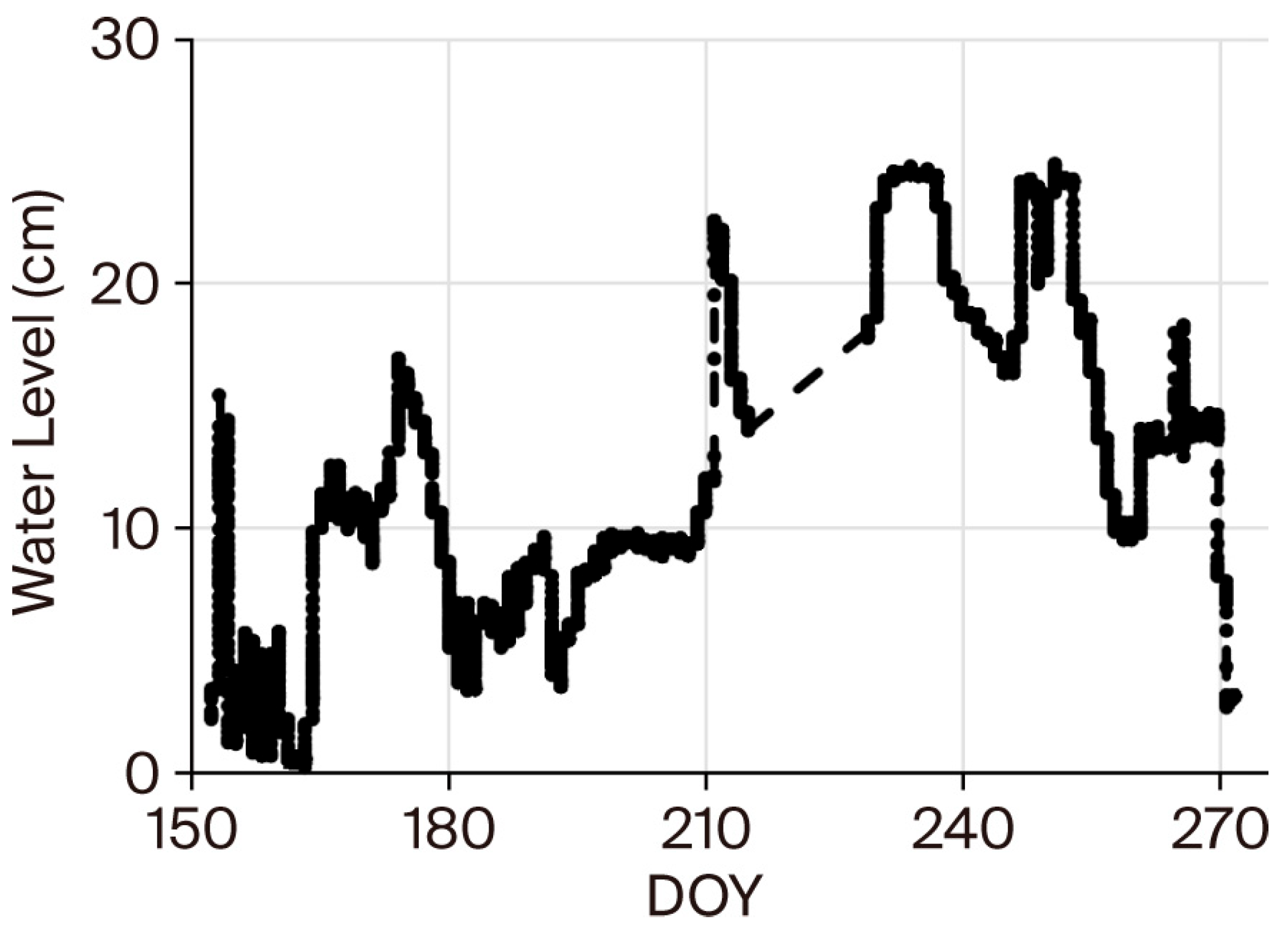
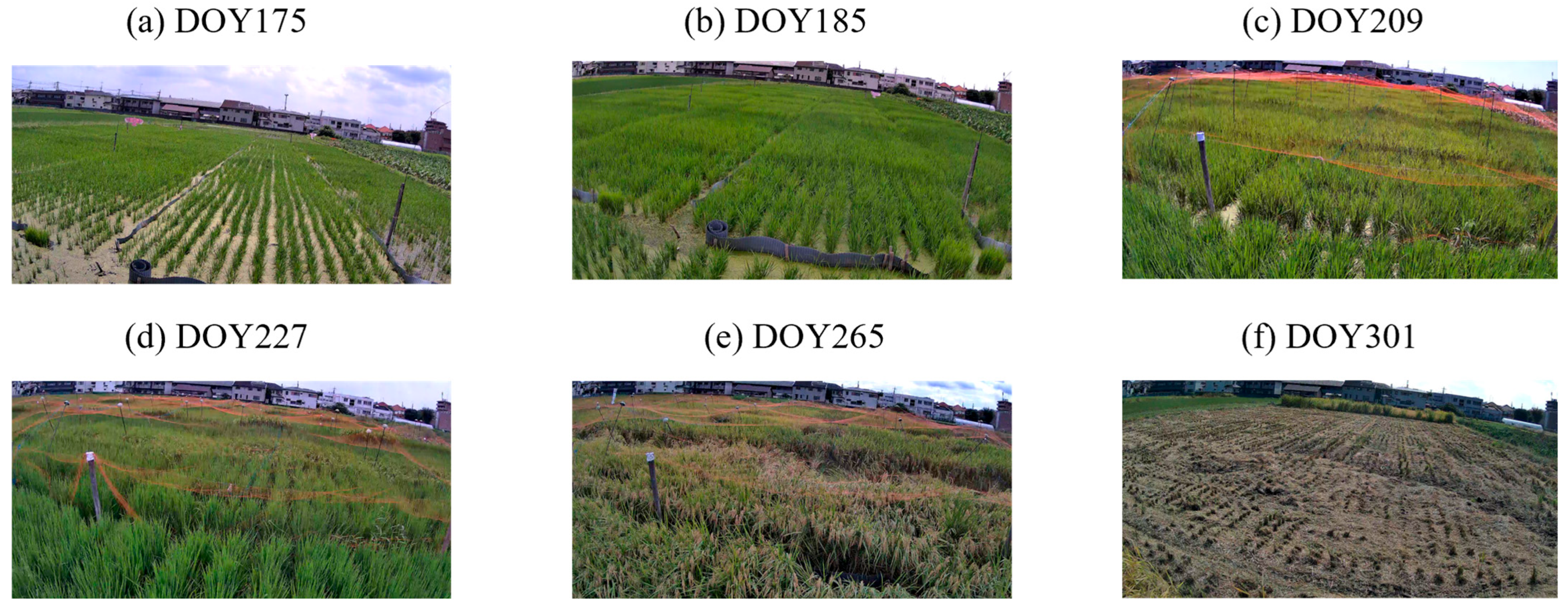
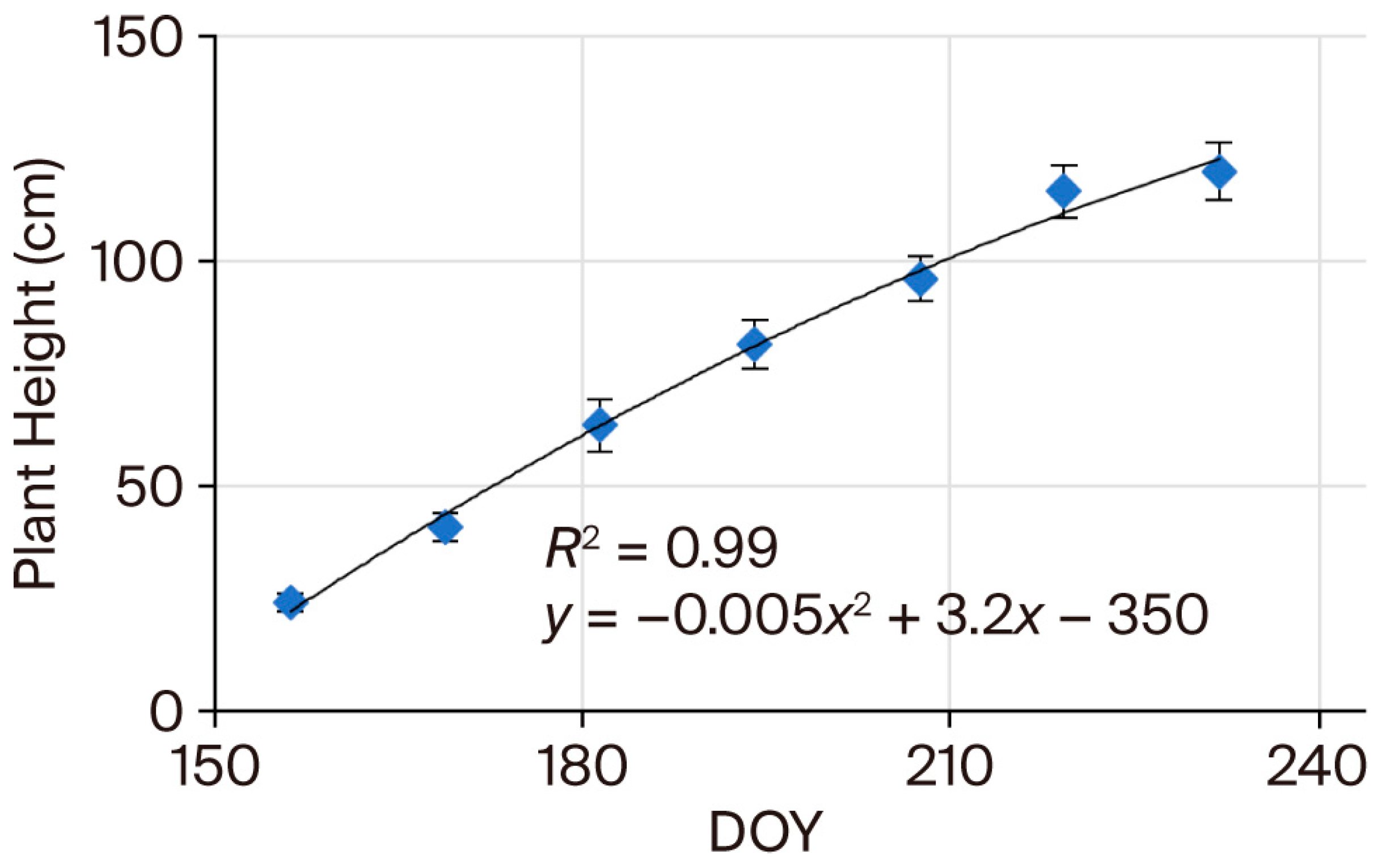
We conducted experiments at a paddy field located in Fuchu, Tokyo, Japan (35.665596°N, 139.471511°E) in 2023. The field was approximately 26 m wide in the east–west direction and 51 m long in the north–south direction. Rice seedlings (Oryza sativa L. cv. Nipponbare) were transplanted on DOY (day of year) 138 and harvested on DOY 300. A resistive water-level sensor (12” long eTape liquid level sensor; Milone Technologies, Inc., Sewell, NJ, USA) was placed within a perforated cylindrical tube installed in the paddy field. Water level was recorded at 30 min intervals using a data logger. On DOY 157, 171, 185, 199, 214, 227, and 241, plant height was measured using a ruler, and the number of tillers per hill was counted using 15 rice hills. In addition, daily time-lapse images of the paddy field were acquired using a time-lapse camera.

2.2. Satellite SAR Observations

In this study, two types of satellite SAR data with different frequency bands and polarization characteristics were used: Sentinel-1A (ESA) and ALOS-2/PALSAR-2 (JAXA). For both satellites, the region of interest (ROI) was defined as the entire paddy field, and the analysis period was set from DOY 152 to DOY 362 to ensure consistency with GNSS-IR and in situ observations. The acquisition conditions and specifications of the SAR data used in this study are summarized in

Table 1. Summary of SAR data acquisition conditions used in this study.

Satellite	Product	Mode	Polarization	Orbit Pass	Look Direction	Incidence Angle (deg)	Pixel Spacing (m)
Sentinel-1A	GRD	IW	VV/VH	Descending	Right	40	10
ALOS-2/PALSAR-2	L2.1	HBQ	HH/HV/VH/VV	Ascending	Left	25–36	6

.

Sentinel-1A is a C-band SAR satellite with a center frequency of 5.4 GHz. In this study, Level-1 Ground Range Detected High-resolution (GRDH) products acquired in Interferometric Wide (IW) mode were used. Dual-polarization data (VV and VH) acquired under descending orbit, right-looking geometry, and an incidence angle of 40° were analyzed. The pixel spacing was approximately 10 m. All processing was conducted using Google Earth Engine (GEE), and we used the backscattering coefficient (σ⁰) products from the Sentinel-1 GRD collection, which are already corrected for orbit, radiometrically calibrated, and terrain-corrected. The σ⁰ values in dB scale were used for the analysis.

ALOS-2/PALSAR-2 is an L-band SAR satellite with a center frequency of 1.2 GHz. In this study, Level-2.1 orthorectified full-polarimetric products (HH, HV, VH, and VV) were used. The observation conditions were ascending orbit with left-looking geometry, and the incidence angle ranged from 25° to 36°. The pixel spacing was approximately 6 m. The data were obtained via the Tellus Satellite Data Platform and processed using QGIS. For the ALOS-2/PALSAR-2 Level-2.1 products, the digital number (DN) was converted to σ⁰ (dB) according to the product specification [46] using Equation (1):

$${\sigma }^0=10{\mathrm{l}\mathrm{o}\mathrm{g}}_{10}\left(\mathrm{D}{\mathrm{N}}^2\right)-83$$

(1)

The objective of this study is to evaluate how differences in observation frequency (C-band versus L-band) and polarization characteristics (co-polarization versus cross-polarization) affect scattering responses in paddy field environments. Therefore, we restricted the analysis to time-series data acquired over the same ROI and focused on comparing the responses of the co-polarized channels (HH and VV), which are generally considered sensitive to surface scattering, with those of the cross-polarized channel (VH), which is considered sensitive to vegetation volume scattering. For monostatic full-polarimetric ALOS-2/PALSAR-2 observations, HV and VH are generally regarded as equivalent under reciprocity; therefore, the use of VH/VV in this study does not imply any essential difference in interpretation from HV/VV. A total of 17 Sentinel-1 scenes and 8 ALOS-2/PALSAR-2 scenes were used in this study. Therefore, the temporal sampling of the SAR observations was much more limited than that of the continuous 1 Hz GNSS-IR observations.

2.3. Ground-Based GNSS-IR Observations

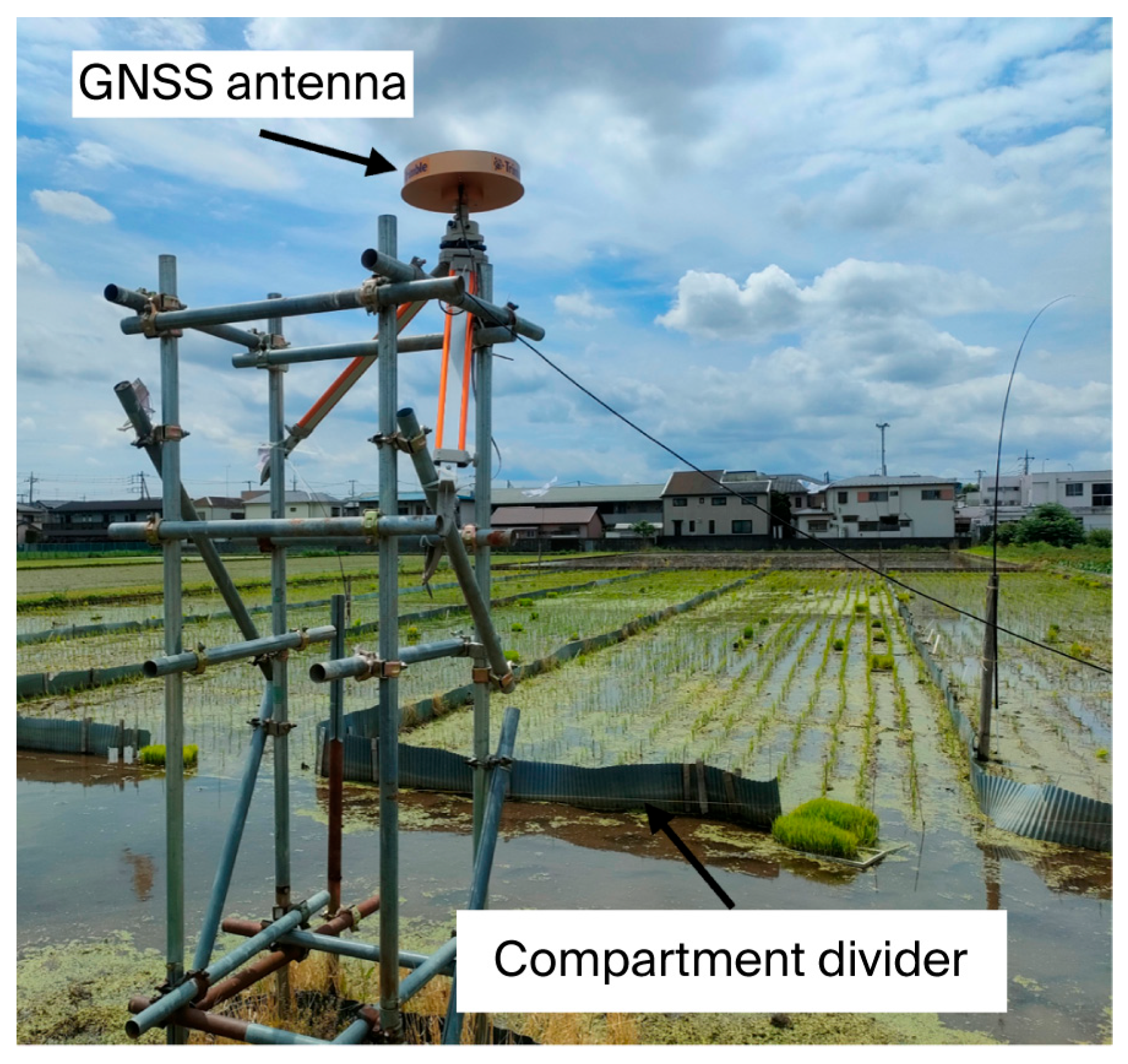
The GNSS antenna was installed at the northern edge of the paddy field, centered in the east–west direction, and fixed at a height of 3.05 m above the ground surface (Figure 1). This configuration results in an observation geometry in which the GNSS-IR analysis primarily targets reflection footprints from satellites moving southward. The equipment consisted of a GNSS receiver (Trimble Alloy) and an antenna (Trimble Choke Ring Antenna v2), both manufactured by Trimble Inc. (Sunnyvale, CA, USA). The observation period was from DOY 152 to DOY 362, and RINEX-format data, including signal-to-noise ratio (SNR), were continuously recorded at a 1 Hz sampling rate. Observations were temporarily suspended between DOY 242 and DOY 252 due to maintenance of the experimental site.

The analyzed signals were the GPS L1 C/A code (center frequency: 1575 MHz) and the L2C signal (center frequency: 1228 MHz). RINEX data were processed using the open-source software gnssrefl (version 2.2.0) [40], which implements GNSS-IR by applying frequency-domain analysis to SNR oscillations observed in low-elevation satellite signals. In this study, gnssrefl was used to derive SNR time series following Equation (2) [47]:

$$\mathrm{S}\mathrm{N}\mathrm{R}=A\mathrm{c}\mathrm{o}\mathrm{s}\left({\displaystyle \frac{4\pi H}{\lambda }}\mathrm{s}\mathrm{i}\mathrm{n}E+\varphi \right)$$

(2)

where $A$ is the amplitude (V/V), $H$ is the distance between the antenna and the reference reflector (cm), $\lambda$ is the wavelength (19.0 cm for L1 and 24.4 cm for L2), E is the satellite elevation angle (degrees), and $\varphi$ is the phase shift (rad).

The SNR data were then restricted to elevation angles between 5° and 45°, and Lomb–Scargle periodogram (LSP) analysis was applied to obtain the spectral power $P_{\lambda }\left(f\right)$ in the frequency domain. The frequency corresponding to the dominant spectral peak $f_p$ is related to the reflector height according to Equation (3) [33]:

$$H={\displaystyle \frac{1}{2}}{f}_p\lambda$$

(3)

Because H represents the distance between the antenna and the effective reflecting surface, the height of the reflecting surface above the ground can be calculated as $h-H$, where h is the known antenna height. This estimated height was compared with the measured water level and vegetation height. According to Fresnel reflection theory, the reflection strength increases with increasing contrast in relative permittivity ($\epsilon$) across an interface. In paddy field environments, the air–water interface (air: $\epsilon \approx 1$; water: $\epsilon \approx 80$) produces the strongest reflection. Therefore, the frequency corresponding to the largest peak in $P_{\lambda }\left(f\right)$ can be interpreted as the case in which the water surface acts as the dominant reflecting surface. We define this frequency as $f_{\mathrm{w}\mathrm{a}\mathrm{t}\mathrm{e}\mathrm{r}}$. Given a known antenna height, Equation (3) enables estimation of water level from $f_{\mathrm{w}\mathrm{a}\mathrm{t}\mathrm{e}\mathrm{r}}$.

In contrast, for herbaceous vegetation, $\epsilon$ of leaves and stems is reported to be typically $\epsilon$ < 40 [48]. As a result, although reflections also occur at air–vegetation interfaces, their reflectivity is weaker than that of the air–water interface. Moreover, unlike the smooth water surface, vegetation consists of complex structures such as leaves and stems, which can induce multiple reflections. Previous studies have suggested that such multiple scattering processes correspond to volume scattering in SAR and are often characterized using cross-polarized channels (HV/VH) [11]. Based on this concept, we assume that GNSS signals in GNSS-IR observations may undergo multiple reflections within the vegetation canopy before reaching the antenna. This assumption implies the existence of multiple effective reflecting surfaces above the water surface. Under this condition, the LSP spectrum is expected to exhibit multiple small peaks in the frequency range below $f_{\mathrm{w}\mathrm{a}\mathrm{t}\mathrm{e}\mathrm{r}}$. Accordingly, we hypothesize that vegetation conditions can be quantified by integrating the spectral power $P_{\lambda }(f,t)$ over the frequency range from a cutoff frequency $f_{\mathrm{m}\mathrm{i}\mathrm{n}}$ to $f_{\mathrm{w}\mathrm{a}\mathrm{t}\mathrm{e}\mathrm{r}}$, as expressed in Equation (4):

$$I_{\lambda }(t)={\int }_{f_{\mathrm{m}\mathrm{i}\mathrm{n}}}^{f_{\mathrm{w}\mathrm{a}\mathrm{t}\mathrm{e}\mathrm{r}}}{P}_{\lambda }(f,t)df$$

(4)

Here, $I_{\lambda }\left(t\right)$ represents the spectral integral at time t for wavelength $\lambda$. Specifically, for each satellite pass in which a rising or setting SNR arc was observed, $I_{\lambda }\left(t\right)$ was calculated by integrating the LSP spectrum between $f_{\mathrm{m}\mathrm{i}\mathrm{n}}$ and $f_{\mathrm{w}\mathrm{a}\mathrm{t}\mathrm{e}\mathrm{r}}$. In GNSS-IR processing, a second-order polynomial detrending is typically applied to remove the slowly varying SNR arc [47]; however, low-frequency residual components may remain. To suppress this residual noise, we introduced the cutoff frequency $f_{\mathrm{m}\mathrm{i}\mathrm{n}}$. In this study, $f_{\mathrm{m}\mathrm{i}\mathrm{n}}$ was set to 10 Hz. From Equation (3), this corresponds to a reflector height of $h-H=210$ cm for the L1 band. Because rice height in the study area does not exceed 200 cm, this value clearly represents an outlier, supporting the appropriateness of this cutoff.

Furthermore, the received GNSS signal power varies day to day due to ionospheric fluctuations and atmospheric attenuation along the signal path. Consequently, the magnitude of $P_{\lambda }\left(f\right)$ also varies between observation dates. To enable comparison on a consistent scale, the spectral integral was normalized by the maximum spectral power at $f_{\mathrm{w}\mathrm{a}\mathrm{t}\mathrm{e}\mathrm{r}}$, yielding the normalized spectral integral defined in Equation (5) as GNSS Phenology Indicator (GPI):

$$\mathrm{G}\mathrm{P}\mathrm{I}={\displaystyle \frac{I_{\lambda }\left(t\right)}{P_{\lambda }(f_{\mathrm{w}\mathrm{a}\mathrm{t}\mathrm{e}\mathrm{r}},t)}}$$

(5)

This normalization reduces the influence of variations in received signal strength caused by ionospheric conditions, atmospheric attenuation, and satellite geometry, enabling comparison across different observation dates. The dominant spectral peak $f_{\mathrm{water}}$ represents the strongest specular reflection from the water surface and is therefore analogous to surface-related scattering observed in SAR co-polarized channels. In contrast, the spectral power below $f_{\mathrm{water}}$, integrated in the GPI definition, reflects attenuation and multiple scattering within the rice canopy, which is conceptually similar to vegetation volume scattering detected by cross-polarized SAR signals. This concept is also analogous to the use of polarization ratios such as VH/VV in SAR analysis, where cross-polarized backscatter is normalized by co-polarized backscatter to suppress observation-dependent variations and emphasize vegetation-related scattering processes.

In this study, GPI was defined as a proxy indicator of vegetation phenological dynamics. Both $f_{\mathrm{w}\mathrm{a}\mathrm{t}\mathrm{e}\mathrm{r}}$ and GPI derived from the LSP analysis were used as GNSS-IR-based indicators and were compared with in situ measurements of water level and rice growth, as well as with SAR-derived metrics.

Finally, to quantitatively evaluate the spatial footprint of GNSS-IR observations, we estimated the footprint size using a geometric model of the first Fresnel zone, as in previous studies [27]. Assuming an antenna height of 3.05 m and elevation angles between 5° and 45°, the distance to the specular reflection point ranged from 3.2 to 47 m for the L1 signal and from 3.2 to 51 m for the L2 signal. These results suggest that both SAR and GNSS-IR observations broadly represent the same experimental paddy field at the field scale.

3. Results

First, the results of in situ measurements of water level and rice growth, which serve as ground truth, are presented. Next, the results of detecting water level dynamics and rice phenological changes using SAR and GNSS-IR observations are described.

3.1. In Situ Measurements at the Study Site

The time series of water level measured using the resistive water level sensor is shown in Figure 2. The water level repeatedly increased and decreased in response to irrigation and drainage, depending on rice growth stages and environmental conditions, and the field was completely drained by DOY 271. Data from DOY 215 to DOY 229 were excluded from further analysis because plant residues clogged the tube housing the sensor, causing the measured water level inside the tube to deviate from the actual water level in the paddy field.

The results of the rice growth surveys are shown in Figure 3. Rice height showed an increasing trend, well approximated by a quadratic curve. The standard deviation also tended to increase with time. Because the coefficient of determination (R²) between the observed heights and the fitted quadratic curve was high (R² = 0.99), this regression model was used to interpolate daily rice height for subsequent comparisons with SAR and GNSS-IR results.

Time-lapse images of the paddy field are presented in Figure 4. Based on Figure 3 and Figure 4, the major phenological events of rice in the study area can be summarized as follows: the maximum tillering stage occurred around DOY 185; heading began around DOY 209; and grain maturation progressed thereafter. Rice harvesting was completed on DOY 301.

3.2. GNSS-IR Spectral Characteristics Revealed by LSP

Analysis of the GNSS observations indicated that the Global Positioning System (GPS) satellite most frequently contributing reflection footprints over the experimental paddy field during the observation period was the satellite with pseudo-random noise (PRN) code 6. Therefore, all results presented in this section are based on data obtained from GPS PRN 6.

To examine the spectral characteristics of GNSS-IR observations, Lomb–Scargle periodograms (LSPs) corresponding to six representative dates (DOYs) shown in Figure 4, which represent different stages of rice phenology, are presented in Figure 5. The observed water level and rice height were converted to theoretical peak frequencies using Equation (3), which were then overlaid on Figure 5.

3.3. Water Level Dynamics Derived from SAR and GNSS-IR Observations

The relationships between the in situ water level measurements and the observations derived from two types of SAR data with different frequency bands, as well as GNSS-IR observations, were examined. The in situ water level was recorded at 30 min intervals, and for each satellite acquisition, the water level measurement closest in time was used for comparison.

We first present the results derived from SAR observations. Although SAR data can be analyzed by polarization, co-polarized channels (VV and HH) are considered more sensitive to surface changes [49]. Therefore, the following analysis focuses on co-polarized backscatter. In the archive for the study area, only VV polarization was available for Sentinel-1A, whereas both VV and HH polarizations were available for ALOS-2/PALSAR-2. Figure 6 shows the relationship between σ⁰ from Sentinel-1A (C-band) and the in situ water level. The correlation between σ⁰ (VV) and water level was weak (r = 0.42).

Figure 7 shows the relationship between σ⁰ from ALOS-2/PALSAR-2 (L-band) and the in situ water level. For VV polarization, a moderate correlation was observed (r = −0.55), whereas a stronger correlation was found for HH polarization (r = −0.77). These results indicate that, in terms of frequency band, L-band backscatter exhibited a stronger relationship with water level than C-band backscatter. Furthermore, within the L-band observations, the correlation with water level was stronger for HH than for VV.

Next, the relationship between GNSS-IR results and the in situ water level is described. Figure 8 shows the relationship between the in situ water level and $f_{\mathrm{w}\mathrm{a}\mathrm{t}\mathrm{e}\mathrm{r}}$, defined as the frequency corresponding to the maximum spectral peak obtained from the LSP analysis of GNSS-IR data. The analysis period was from DOY 175 to DOY 273. The values on DOYs 175 and 176 were outliers compared with the other observations. After excluding these two outliers, the correlation coefficients were r = −0.63 for L1 and r = −0.76 for L2, indicating that the lower-frequency L2 signal showed a stronger relationship with water level than L1.

3.4. Phenological Dynamics Derived from SAR and GNSS-IR Observations

Figure 9 shows the relationships between the time series of phenological indicators derived from SAR and GNSS-IR and the rice growth stages. For SAR, the VH/VV ratio calculated from σ⁰ for each polarization was used as the phenological indicator, following previous studies [11]. For GNSS-IR, the GPI calculated using Equation (5) was used as the phenological indicator. The major growth stages identified based on Figure 3 and Figure 4 were overlaid on the time series.

GPI gradually increased from the vegetative growth stage to the heading stage, reached high values around the heading period, and then decreased during the grain-filling stage. A sharp change was also observed around the harvest period. The SAR-derived indicator exhibited a similar tendency, with relatively high values around the heading stage and a decreasing trend thereafter. In particular, the L-band SAR indicator showed an increasing trend similar to that of GPI, whereas the C-band SAR indicator exhibited a decreasing trend, unlike both L-band SAR and GPI. The change associated with harvesting was more clearly observed in GPI than in the SAR indicator.

In addition, as shown in Figure 9b, the temporal rate of change (first derivative) of GPI exhibited pronounced peaks around the heading period and the harvest period. These results indicate that the GPI is sensitive to rice phenological changes, similarly to the SAR-based phenological indicator VH/VV. Figure 9c, together with the photographic record in Figure 4, indicates that the seasonal evolution of GPI corresponded well to the progression of rice phenology. The temporal pattern was also broadly consistent with that of the SAR-based indicator, supporting the correspondence between the GNSS-IR-derived GPI and the SAR observables related to rice growth.

To assess the sensitivity of the proposed indicator to the choice of cutoff frequency $f_{\mathrm{m}\mathrm{i}\mathrm{n}}$ in the definition of the normalized spectral integral, a sensitivity analysis was conducted for three values: $f_{\mathrm{m}\mathrm{i}\mathrm{n}}=5$, 10, and 15 Hz. The overall temporal patterns were consistent across all three conditions, confirming that the indicator used in this study is robust to the choice of $f_{\mathrm{m}\mathrm{i}\mathrm{n}}$ (Figure A1).

4. Discussion

4.1. Interpretation of LSP Spectra in GNSS-IR

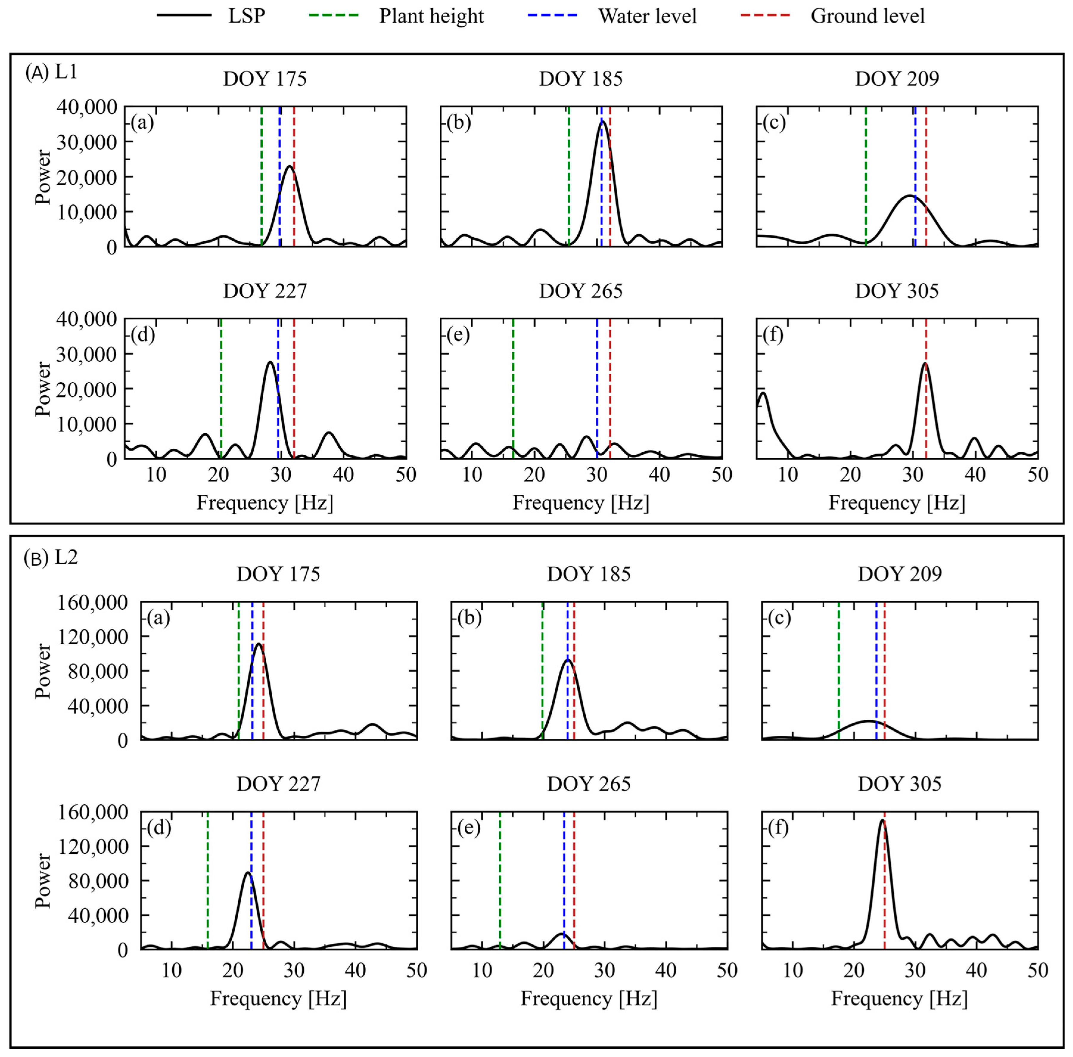
In GNSS-IR, the dominant reflector height corresponding to specular reflection can be extracted by representing the frequency components of SNR oscillations using the Lomb–Scargle periodogram (LSP) (Equation (3)) [33]. In environments with a water surface, such as paddy fields, a smooth air–water interface tends to produce a distinct, sharp spectral peak. As vegetation develops, however, signal attenuation and scattering increase, which can reduce peak amplitude and lead to a more complex spectral structure, including peak broadening and the emergence of multiple peaks.

In this study, the LSP spectra changed systematically from a simple peak structure in the early flooded stage to broader or multiple-peak structures in the later growth stages. These changes can be interpreted as a transition from conditions in which the water surface acts as a clear, dominant reflecting interface to conditions in which vegetation-induced attenuation and scattering become more influential, resulting in mixed and unstable effective reflectors.

As vegetation growth attenuates the specular reflection component from the water surface, the LSP peak becomes relatively weaker, and peak broadening (i.e., increased uncertainty in the effective reflector height) and the appearance of multiple peaks (i.e., multiple effective reflecting surfaces) become more likely. Furthermore, this study showed that the L1 signal tended to exhibit more small peaks, whereas the L2 signal showed a simpler spectral structure. This difference may reflect wavelength-dependent differences in scattering sensitivity and penetration behavior within the rice canopy. However, quantitative verification of this mechanism, including penetration-depth estimation based on canopy dielectric properties and stage-dependent comparison of L1/L2 spectral characteristics, remains for future work.

4.2. Water Level Detection by SAR and GNSS-IR

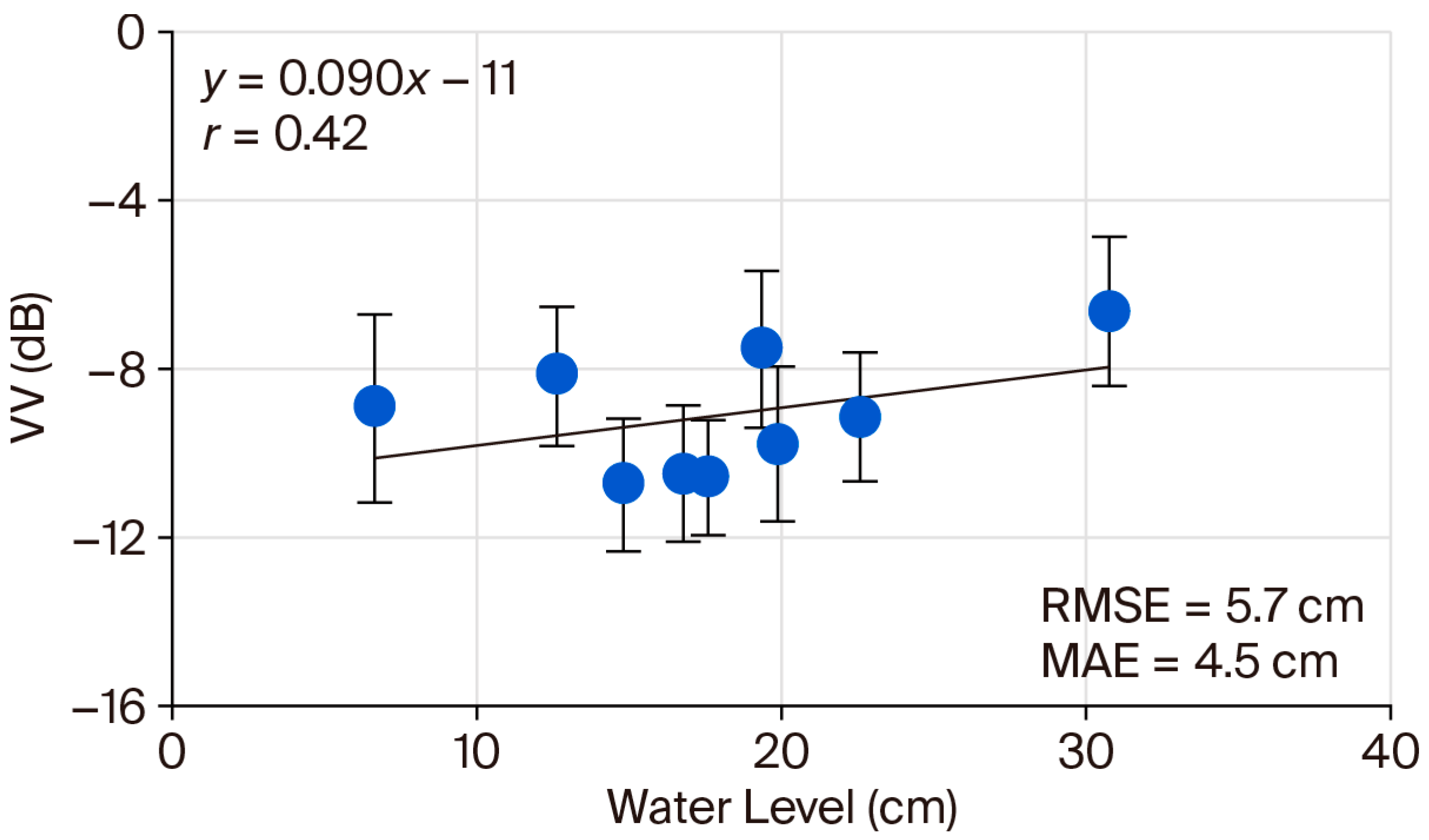
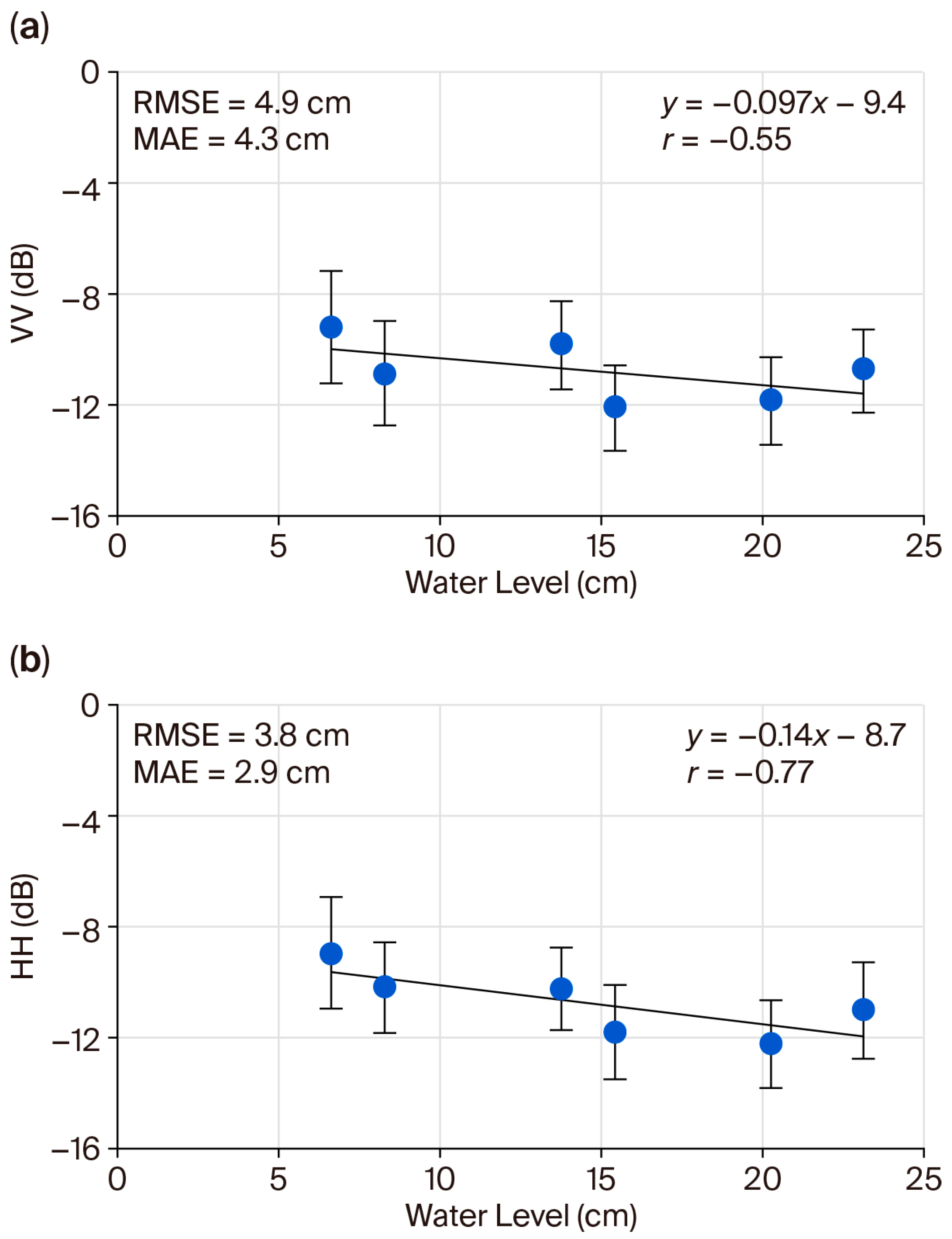
The weaker response of Sentinel-1A C-band VV backscatter to water level can be interpreted mainly by limited penetration into the rice canopy and by the mixed nature of the backscattered signal. In flooded rice fields during the growing season, SAR backscatter is influenced not only by the water surface but also by stems, leaves, vegetation water content, and observation geometry [20]. Under such conditions, the C-band signal is more strongly affected by vegetation elements and is therefore more likely to lose direct sensitivity to water-level fluctuations. In contrast, L-band signals can penetrate the canopy to some extent and thus retain greater sensitivity to the flooded surface. Previous studies have also reported that L-band polarimetric information, particularly indicators of double-bounce scattering, can contribute to the discrimination of flooded conditions even at advanced rice growth stages [18,19]. The opposite signs of the correlation coefficients for C-band and L-band may be related to the different scattering sensitivities associated with their wavelengths. In flooded rice fields, L-band signals can penetrate the rice canopy and may be influenced by reflections from the water surface, whereas C-band signals interact more strongly with vegetation elements such as rice stems and leaves.

The stronger relationship between water level and HH than VV in L-band SAR may be related to polarization-dependent scattering and attenuation behavior under flooded rice-field conditions. Previous studies have reported that, under double-bounce conditions, VV can become relatively lower than HH and may be more susceptible to attenuation effects [14]. However, quantitative verification of this mechanism, including estimation of polarization-dependent attenuation and its relationship to rice height and biomass, remains for future work.

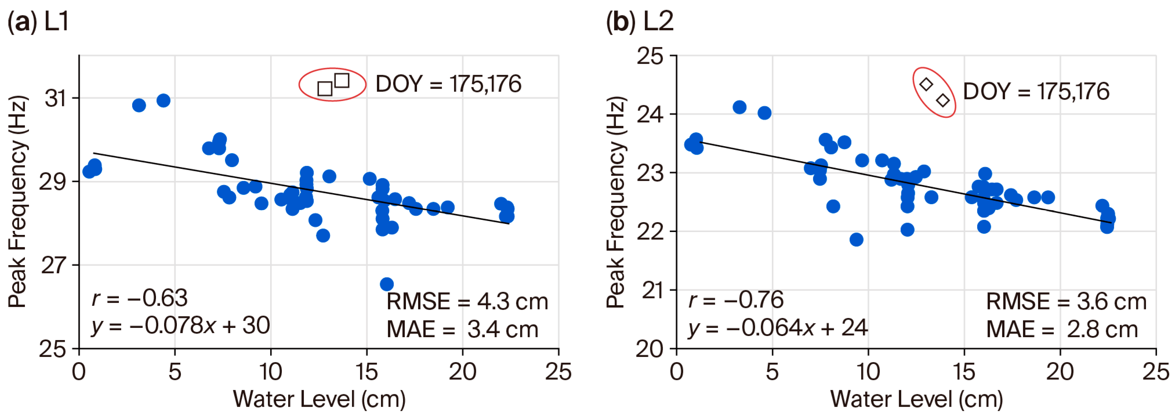
GNSS-IR also exhibited a negative correlation between the water-surface-related peak frequency $f_{\mathrm{w}\mathrm{a}\mathrm{t}\mathrm{e}\mathrm{r}}$ and the in situ water level, with a particularly strong correlation for L2 (r = −0.76), indicating that water-level estimation based on the water-surface peak is feasible under certain conditions. During DOY 175–176, the dominant spectral peak appeared between the theoretical frequencies corresponding to the water surface and the ground surface (Figure 5). This resulted in the height outliers shown in Figure 8.

Because L-band signals can penetrate rice canopies to some extent, as demonstrated in this study and previous work [18], two signal paths are expected when L-band electromagnetic waves impinge on the water surface: (i) reflection from the water surface followed by re-reflection from vertically oriented rice structures, and (ii) transmission through the canopy and radiation upward toward the antenna. The former path is likely captured by the double-bounce component in co-polarized SAR backscatter (HH and VV), whereas the latter path is captured by the signal received by the GNSS antenna. In this sense, both the SAR co-polarized backscatter and the GNSS-IR-derived $f_{\mathrm{w}\mathrm{a}\mathrm{t}\mathrm{e}\mathrm{r}}$ reflect a common physical phenomenon: strong reflection originating from the water surface.

4.3. Detection of Phenological Changes by SAR and GNSS-IR

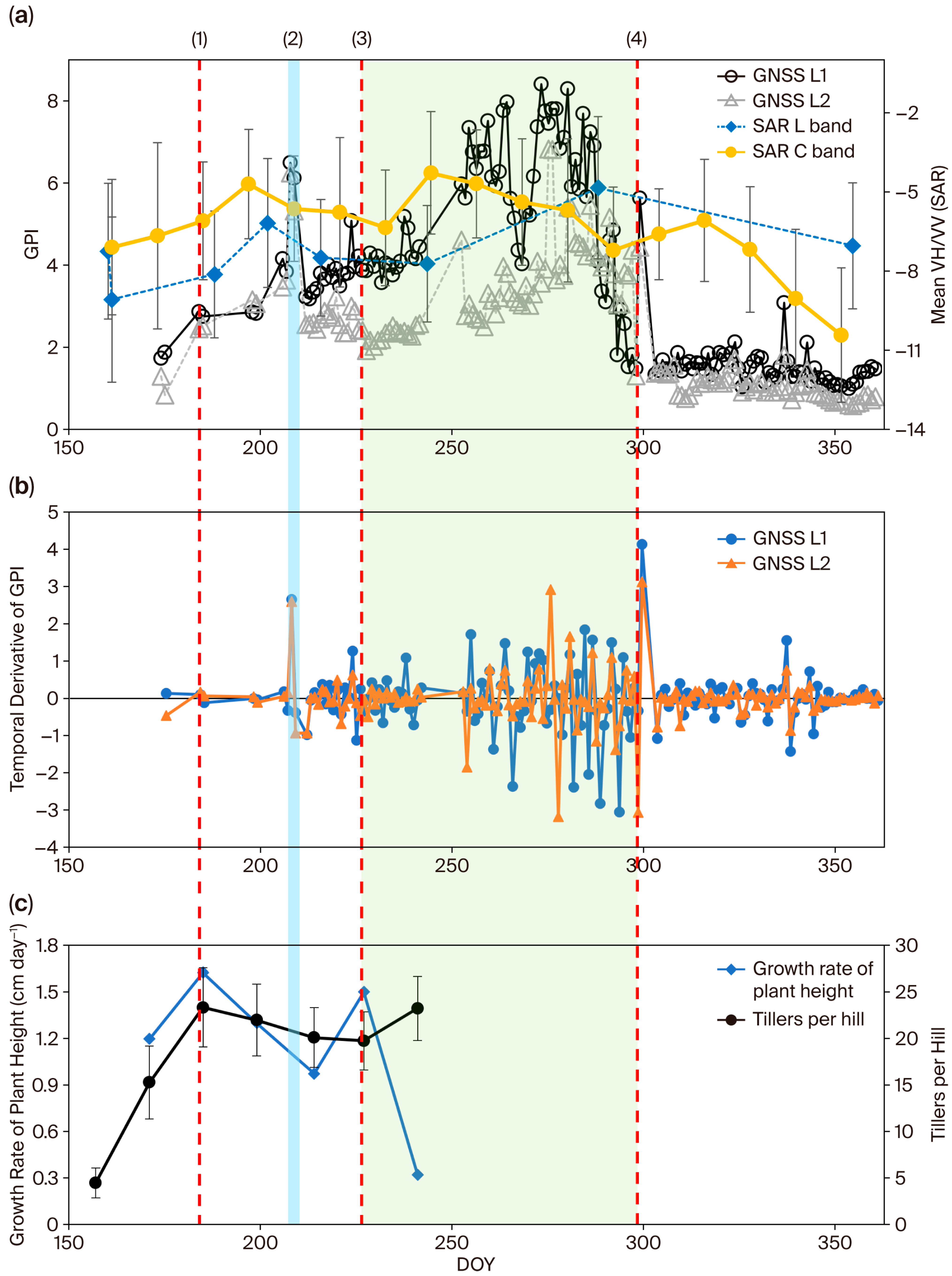
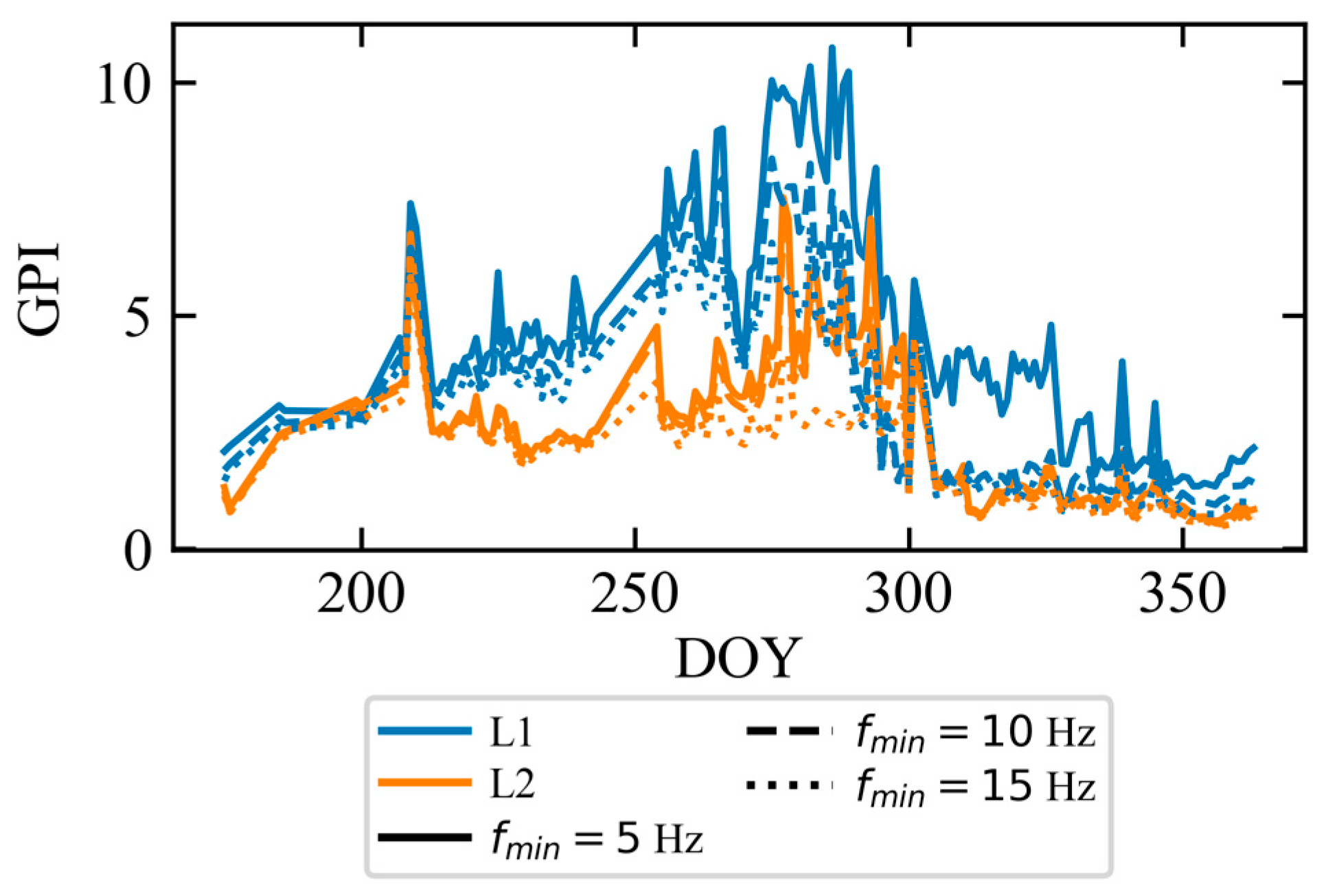
In this study, the GPI was defined as a phenological indicator (Equation (5)), and its sensitivity to phenological changes was demonstrated (Figure 9). This result suggests that the increase in canopy-induced attenuation and scattering associated with rice growth is reflected in enhanced spectral power below $f_{\mathrm{w}\mathrm{a}\mathrm{t}\mathrm{e}\mathrm{r}}$, indicating the potential of GNSS-IR as a ground-based L-band monitoring approach for tracking vegetation phenology.

The differences between the C-band and L-band SAR phenological indicators may be explained by wavelength-dependent sensitivity to canopy structure. If C-band signals are more sensitive to upper-canopy components, such as panicles and leaves, whereas L-band signals are more sensitive to lower-canopy components, such as stems, then C-band observations would be more affected by geometric changes associated with panicle drooping, whereas L-band observations would capture structural changes related to stem elongation and tiller dynamics.

The GPI exhibited temporal variations like those of the ALOS-2/PALSAR-2 VH/VV ratio. In addition, the GPI showed higher sensitivity for L1 than for L2 after the heading stage, as reflected by larger GPI values, suggesting greater sensitivity to mature rice. This difference can also be attributed to wavelength-dependent penetration effects. Furthermore, changes associated with harvesting (DOY 301) were more clearly detected by GNSS-IR than by SAR. GNSS-IR is known to be highly sensitive to changes in reflector height [27,29,50], and the results of this study indicate that the presence or absence of rice was successfully captured as a height-related change.

Previous studies on rice phenology using Sentinel-1A [11] have reported that VV responds to a mixture of vegetation scattering, surface scattering, and double-bounce scattering, whereas VH is primarily associated with vegetation volume scattering, making VH/VV a robust vegetation indicator. The seasonal variation in VH/VV may also be influenced by attenuation (extinction) of the VV component caused by the vertically structured rice canopy. Therefore, the dynamic range of VH/VV should be interpreted not only in terms of increased cross-polarized scattering, but also in relation to polarization-dependent attenuation within the canopy. Thus, SAR detects rice phenological changes primarily through variations in volume scattering. In contrast, GPI integrates spectral power below $f_{\mathrm{w}\mathrm{a}\mathrm{t}\mathrm{e}\mathrm{r}}$, effectively capturing multiple reflections analogous to volume scattering. Therefore, both the SAR cross-polarization channel (VH) and GPI are theoretically sensitive to volume scattering, and the present experiment provides empirical support for this interpretation.

The marked decrease in GNSS L1 GPI during the grain-filling and maturity period likely reflects senescence of the rice canopy after heading. As the canopy dries and vegetation water content decreases, microwave attenuation and multiple scattering within the canopy are reduced, leading to lower GPI values. In addition, the relatively low and stable GNSS-IR metrics observed after harvesting can be interpreted as a reference level under minimal vegetation influence.

4.4. Physical Correspondence and Integration Potential of SAR and GNSS-IR

The results of this study suggest a consistent interpretation of microwave scattering processes in rice paddies when combining SAR and GNSS-IR observations. Water-level variations are primarily captured by the dominant GNSS-IR spectral peak ($f_{\mathrm{w}\mathrm{a}\mathrm{t}\mathrm{e}\mathrm{r}}$), which corresponds to strong reflections from the water surface. Similarly, L-band SAR co-polarized backscatter is sensitive to surface-related scattering associated with the water surface. In contrast, vegetation development influences the GNSS-IR spectrum through attenuation and multiple scattering within the canopy, which is represented by the proposed GPI. This process is analogous to vegetation volume scattering detected by SAR cross-polarized signals.

Both the co-polarized L-band SAR backscatter (VV and HH) and the GNSS-IR-derived LSP peak frequency $f_{\mathrm{w}\mathrm{a}\mathrm{t}\mathrm{e}\mathrm{r}}$ exhibited comparable correlations with water level, indicating that both approaches are sensitive to water-level variations. In addition, the L-band SAR volume-scattering-related indicator (VH/VV) and GPI exhibited similar temporal dynamics and were sensitive to rice phenological changes. These findings demonstrate that GNSS-IR, as a ground-based microwave-scattering observation technique, can provide complementary information useful for the physical interpretation of SAR observations.

A practical advantage of GNSS-IR lies in its high temporal resolution. The number of operational L-band SAR satellites is limited, which constrains observation frequency. In contrast, GNSS constellations such as GPS consist of numerous satellites, enabling high-frequency monitoring. In this study, all available SAR archive data were used, yet the number of SAR observations remained limited, whereas GNSS-IR provided dense time series. This highlights the practical utility of GNSS-IR for continuous monitoring.

Although this study focused on rice and paddy field environments, the proposed framework may also be applicable to other vegetation types and non-flooded soil surfaces. For example, in soil moisture estimation over vegetated surfaces, separating the effects of vegetation and soil moisture remains a major challenge [32,51]. As shown in Equation (2), GNSS-IR SNR contains information on amplitude (reflection strength), frequency (reflector height), and phase (propagation delay) as a function of elevation angle, and LSP analysis enables visualization of energy distribution in the vertical dimension (Figure 5). This principle underlies previous demonstrations that GNSS-IR can be used to estimate microwave penetration into vegetation [37,38] and into soil [35]. In contrast, SAR backscatter represents a single observation at a fixed off-nadir angle, resulting in a mixed signal influenced by vegetation, surface roughness, and soil moisture [52], making vertical separation inherently difficult. Therefore, the integration of SAR and GNSS-IR proposed in this study is advantageous in that GNSS-IR can complement SAR by providing vertical structural information that is not accessible from SAR alone. Future work integrating SAR and GNSS-IR is expected to advance understanding of radar scattering and reflection characteristics of land surfaces, particularly at L-band frequencies.

It should also be noted that a direct quantitative comparison with existing rice monitoring studies based on single SAR, single GNSS-IR, or optical remote sensing is not straightforward, because the target variables and evaluation metrics differ among studies. Many previous studies have emphasized classification accuracy, phenological stage estimation, or mapping performance, whereas the present study focuses on the physical correspondence of SAR and GNSS-IR indicators for water-level and phenological monitoring. In addition, direct comparison is further complicated by differences in observation conditions among studies, including meteorological conditions, paddy-field environments, rice cultivars, and observation periods. Therefore, the main contribution of this study is not to claim superior accuracy over existing single-sensor approaches, but to demonstrate the complementary value of integrating spaceborne SAR with continuous ground-based GNSS-IR observations through a physically consistent interpretation framework. A more rigorous quantitative comparison across different sensing approaches remains for future work.

It should also be noted that the comparison between SAR and GNSS-IR in this study was conducted at the field scale rather than as a strict point-to-pixel correspondence. Although the GNSS-IR footprint and the SAR ROI both covered the experimental paddy field, an explicit spatial matching analysis, such as point-to-pixel overlap evaluation, was not performed and remains for future work.

5. Conclusions

This study investigated the relationships between satellite SAR observations (Sentinel-1 C-band and ALOS-2/PALSAR-2 L-band) and ground-based GNSS-IR measurements over a paddy field, with the aim of interpreting their responses to water level variations and rice phenological dynamics within a consistent physical framework. GNSS-IR SNR data were analyzed using Lomb–Scargle periodogram (LSP) analysis, and two indicators were evaluated: the dominant spectral peak frequency $f_{\mathrm{w}\mathrm{a}\mathrm{t}\mathrm{e}\mathrm{r}}$ related to the water level and GPI, representing vegetation-induced scattering and attenuation effects.

The main findings can be summarized as follows. First, the shape of GNSS-IR LSP spectra evolved systematically with phenological progression. During the early flooded stage, a clear and sharp spectral peak was observed, whereas peak weakening, broadening, and the emergence of multiple peaks occurred as vegetation developed. These spectral changes are consistent with increasing attenuation and multiple scattering within the canopy. Differences between L1 and L2 signals further suggest wavelength-dependent sensitivity to canopy structure.

Second, for water level variations, the co-polarized L-band SAR backscatter (VV and HH) and the GNSS-IR spectral peak frequency exhibited comparable relationships with in situ water level, whereas C-band SAR VV backscatter showed weaker sensitivity. This suggests that both L-band SAR and GNSS-IR retain sensitivity to water surface conditions even under developing vegetation.

Third, for phenological dynamics, GPI exhibited temporal variations comparable to those of the SAR-based polarization ratio (VH/VV), including clear responses around heading and harvest periods. The temporal derivative of GPI further highlighted transitions between major growth stages, indicating sensitivity to phenological change.

Overall, these results support the interpretation that L-band SAR co-polarized responses correspond to water-surface-related GNSS-IR components, whereas SAR cross-polarized indicators correspond to vegetation-related spectral components in GNSS-IR. Because GNSS-IR provides dense temporal sampling and contains information on vertical structure that is difficult to retrieve from SAR alone, integrating SAR and GNSS-IR offers a promising framework for a more physically grounded interpretation of microwave interactions with land surfaces.

A practical application of the proposed framework is representative-field-based monitoring for paddy water management. Continuous GNSS-IR observations at a representative field can provide high-temporal-resolution information on local water-level and phenological changes, while SAR observations can extend these physically interpreted indicators to surrounding fields without requiring antenna installation in each field. Such a framework could support irrigation and drainage management, detection of delayed field operations, and regional assessment of paddy-field conditions.

Although this study was conducted at a single site and for a single growing season, the objective was not to establish a generalized retrieval algorithm but to demonstrate the physical consistency between SAR scattering mechanisms and GNSS-IR spectral behavior. Future work should focus on validation across multiple sites and years, the development of quality-control strategies for dense vegetation conditions, and the extension of the framework to other applications, such as soil moisture estimation and vegetation monitoring.