


Highlights
What are the main findings?
- Machine learning models applied to drone imagery accurately mapped nine distinct salt marsh communities (average 94.7%).
- Photogrammetric DSMs were the most important feature, highlighting the value of elevation in salt marsh habitat classification.
What are the implications of the main findings?
- Combined UAV and machine learning tools provide an excellent method for monitoring restoration success in salt marshes.
- UAV mapping of standardised plant communities could provide valuable data for biodiversity assessments and ecosystem service accounting.
Abstract
Species composition is an important indicator for the condition, functioning, and ecosystem service provision of salt marshes, making the mapping of species composition valuable for their management. Previous studies have demonstrated that the combined use of unoccupied aerial vehicle (UAV)-mounted multispectral cameras and machine learning (ML) can provide effective mapping of vegetation communities in these habitats. However, to date, these studies have predominantly focused on relatively species-poor salt marshes in North America. There has been no published testing of these combined UAV-ML methods in the salt marshes of northwestern Europe, which contain different often more diverse assemblages. Consequently, this study investigated whether applying recent methodological advances can accurately map National Vegetation Classification communities in three locations in the United Kingdom, each comprising two salt marsh sites, one established and one restored. Sites consisted of a mix of established and restored salt marshes of different ages, enabling a complementary assessment of how these methods perform in communities at different stages of development. The applied random forest ML models were found to produce highly accurate maps of salt marsh vegetation communities, with a mean overall accuracy of 94.7%. No relationship was found between the age of restoration sites and the accuracy of the classifications, showing these methods may be applied at a range of stages of community development and offer wider applicability for saltmarsh management and monitoring. The findings of this study demonstrate that advances in the combined use of drones and machine learning provide a readily transferrable method for mapping standardised vegetation communities in both established and restored northwestern European salt marshes and therefore likely other salt marshes globally. Consequently, this study demonstrates that both researchers and practitioners may confidently use these methods to create improved assessments of both marsh condition and function.
1. Introduction
Salt marshes are recognised for providing a wide range of ecosystem benefits such as flood and wave attenuation [1,2] and carbon sequestration [3,4]. Growth in the appreciation for the value of salt marshes has led to both protection and restoration policies that have in turn intensified demands on monitoring protocols [5]. Vegetation is the dominant biotic component of these marshes, and thus, the different functional traits of species are critical to a marshes’ overall function [6,7], with the provision of ecosystem benefits varying between species assemblages [8,9]. Species composition has also been shown to be an indicator of surface elevation change in marshes [10,11], a critical factor in determining their resilience relative to sea level rise [12,13]. As a result, species composition is a valuable and widely used indicator for monitoring both salt marsh condition and function [14,15], including measuring adherence to conservation policies [16,17].
A common method for summarising variations in species composition is to describe species that are frequently found together as belonging to a community. Plant communities can be readily identifiable in salt marshes, as species tend to group by their tolerance to tidal inundation and salinity, which form strong gradients within the intertidal zone [18,19,20,21]. In the United Kingdom (UK), a national standard for vegetation communities was determined in the National Vegetation Classification (NVC) [22]. The NVC is the result of extensive vegetation surveys across the range of habitats found in Great Britain in the 1970s, with the data then grouped into nationally relevant communities using multivariate statistics. Such standardised communities provide a unified method for describing species composition between sites. This has led to the NVC becoming widely used for describing species composition in the UK across both science [23] and environmental management [17,24,25,26,27], making the mapping of NVC communities valuable for both applications. Comparable classification schemes have also been developed in other areas of the world, such as the EUNIS classification, which is used across the European Union [28], and the United States NVC (USNVC) in the United States of America [29].
Traditional in situ field surveys are extremely challenging, time-and resource consuming, and potentially damaging in dynamic and fragile habitats such as coastal wetlands [30,31], limiting the feasibility and desirability of frequent large-scale analyses of coastal plant communities [15,32,33,34,35]. Comparatively, remote sensing tools offer many benefits for environmental monitoring. Firstly, remotely sensed images provide a spatially comprehensive view of a system, which is often more representative than point-based in situ samples [36]. This comprehensive view can become especially important in intertidal systems, where sites may not be widely accessible for field surveys due to safety concerns and designations [37,38,39]. Secondly, the repeatable nature of remote sensing allows the tracking of temporal shifts of species composition, such as post-restoration trajectories.
The potential for remote sensing to provide valuable data about salt marshes has been demonstrated with satellites [40,41,42,43]. However, the fine-scale heterogeneity of species composition in salt marshes can be challenging to map at satellite resolutions [42]. Comparatively, unoccupied aerial vehicles (UAVs, also known as drones or UA Systems (UAS)) can fly close to the ground surface, providing ultra-high spatial resolution at a low cost (especially when compared to plane-based surveys) [44,45,46]. Additionally, the low flight height of UAVs means images of the ground surface can be captured during clouded conditions, while their low cost also means they can be flown with flexible repeat times [44].
A current state-of-the-art method for mapping vegetation communities with UAVs involves the use of multispectral sensors, which capture reflectance in discrete wavelength regions. Multispectral imagery can be combined with other features such as a Digital Elevation Model (DEM) and texture to build a machine learning (ML) classifier. The effectiveness of this approach in salt marshes has been demonstrated in the USA [45,47,48,49,50], Canada [51,52], and China [53]. However, these prior studies have predominantly focussed on communities with little plant species diversity, many being monospecific stands. Comparatively, salt marshes of northwestern Europe are considerably more diverse [54]. This higher diversity may reduce the effectiveness of this method in the region. Higher species diversity has been suggested to increase spectral variability, weakening relationships between spectral reflectance and vegetation units and thus reducing classification accuracies [55]. However, a key knowledge gap remains, as this method has not been tested in these systems, and its performance under more diverse conditions is therefore uncertain.
Research that has explored the use of remote sensing to map vegetation communities within salt marshes in northwestern Europe was carried out by Thomson et al. [56,57,58] and Friess et al. [36]. These studies achieved overall accuracies of around 70%, substantially lower than the often 90+% accuracies achieved by studies using UAVs elsewhere across the globe [50,51,52]. However, they utilised an aeroplane-mounted CASI (Compact Airborne Spectrographic Imager) multispectral camera with a resolution of c. 2–4 m. This resolution is far coarser than the centimetre-scale imagery available from UAVs, with the finer resolution of UAV imagery shown to improve classification accuracies [44]. In addition, these studies relied on multispectral bands and vegetation indices and did not make use of data fusion techniques such as including digital surface models (DSMs) and textural features. These features can provide valuable information to determine classifications. Elevation models incorporate the typically strong relationships between zonation and elevation due to tidal inundation [59]. Furthermore, textural features incorporate information about conditions in adjacent pixels, which can quantify differences in the shape of cover types [60]. Both textural and elevation features have previously been shown to improve classification accuracies for vegetation communities in coastal wetlands for these reasons [50,51].
This study explores whether advances in remote sensing such as UAVs and data fusion can be used to improve the classification of NVC communities in salt marshes. This assessment was applied in both restored and established UK salt marshes. The objectives of this study were to (a) develop maps of NVC communities across UK salt marsh study sites using ML applied to UAV imagery, (b) assess the accuracy of the derived maps using independent validation data, and (c) assess the importance of the features included in the model for determining final model accuracies. This study concluded that the combined use of UAVs and ML can produce accurate maps of plant communities in the coastal wetlands. This finding demonstrates that spatially comprehensive maps of standardised vegetation communities can effectively be created with these tools, providing improved data for biodiversity assessments and ecosystem service accounting.
2. Materials and Methods
2.1. Study Sites
This study was based in three different locations in southern England in the United Kingdom (UK): Abbotts Hall, Cobnor Point, and the Adur Estuary (Figure 1). All three locations contain both a restored salt marsh site and a nearby established salt marsh site, creating a total of six sites. The restored sites were created through the managed realignment of sea defences in each of the sites, with Abbotts Hall realigned in 2002, Cobnor Point in 2013, and the Adur Estuary in 2019. The three locations fall within the southeastern type of salt marsh vegetation in the UK [61].
Figure 1.
The three study locations in the United Kingdom with their restored and established study sites. Vector outlines (a) are sourced from the Ordnance Survey Boundary Lines dataset [62]. Aerial imagery (b–d) was sourced from the Channel Coastal Observatory (http://www.channelcoast.org). All maps are north oriented.
2.2. Data Collection
2.2.1. Ground-Truth NVC Communities and Additional Cover Types
Repeated ground-truth samples of NVC communities were collected in field surveys carried out in the summer (June/July) over three years (2021–2023) in the Adur Estuary sites, and surveys in the Cobnor Point (July) and Abbotts Hall (August) sites were conducted in the summer period in 2023. A total of twelve 2 m by 2 m quadrats were laid in each of the observed communities on the sites. Species percentage cover was recorded in each of the quadrats, with the quadrats then assigned to the NVC community with the highest similarity using the RMAVIS software (version 1.0.1; UK Centre for Ecology and Hydrology, Wallingford, UK) [63]. A description of these communities is given in Table 1. The location of each of the quadrats was recorded using a differential GPS (dGPS; Leica GS10 and CS15; Leica Geosystems, St. Gallen, Switzerland) by marking each of the four corners of the quadrat. These were digitised as polygons and labelled with the NVC community.
Table 1.
National Vegetation Classification (NVC) communities used in this study. The codes for the communities are given along with a description of the communities taken from Rodwell et al. [22], with the nomenclature adapted to fit conventions outlined in the latest edition of Stace [64].
To ensure class balance, 12 quadrats were used for creating the training/testing data. However, due to the post hoc assignment of communities from the species composition data, this was not always the case. In some cases, communities were merged leading to a larger number of quadrats. In this case, the quadrats were subsampled to achieve the target of 12 quadrats. This subsampling was not performed randomly. Instead, non-metric multidimensional scaling (NMDS) was performed on the species composition data using the vegan package in R [65] with Bray–Curtis dissimilarity. Centroids were created for each of the communities, with the 12 quadrats with the shortest distance to the centroid chosen. This approach was used to ensure that the 12 chosen quadrats were the best available representatives of cover within the community and therefore were assumed to contain the “purest” pixels.
Although not a cover type, shadows were also added for one of the surveys (Cobnor Point established) that contained shadowed areas due to being carried out later in the day.
2.2.2. Aerial Surveys
Aerial surveys of the Adur Estuary, Cobnor Point, and Abbotts Hall sites were carried out using Unmanned Aerial Vehicles (UAVs). Surveys were carried out in the Adur Estuary in the summer (June/July) of 2021, 2022, and 2023. Surveys of Cobnor Point and Abbotts Hall were carried out in the summer (July/August) of 2023. All flights were carried out at low tide and in clear sky conditions. Full details of flight dates are given in Appendix A. In total, this consisted of seven flights, three in the Adur Estuary (where both the restored and established marsh could be captured in one flight) and two at both the Cobnor Point and Abbotts Hall locations (where the new and established sites were captured in separate flights).
Two different UAVs were used: a SenseFly eBee Plus fixed-wing UAV (EagleNXT, Allen, TX, USA) (hereafter referred to as the eBee) and a DJI Matrice 600 Pro multi-rotor UAV (SZ DJI Technology Co., Ltd., Shenzhen, China) (hereafter referred to as the M600). The eBee was used for the surveys in 2021, while the M600 was used for the 2022 and 2023 surveys to make use of its more manoeuvrable multi-rotor capabilities adjacent to an airport, where the Adur study was conducted. Both UAVs were equipped with a Parrot Sequoia multispectral camera (Parrot S.A., Paris, France) (hereafter Sequoia) that was mounted at nadir. This sensor features a 1.2-megapixel narrow-band camera, which captures images in the green (G, 530–570 nm), red (R, 640–680 nm), red-edge (Redg, 730–740 nm), and near-infrared (NIR, 770–810 nm) wavelengths. Red–green–blue (RGB) images were also collected during each of the surveys for visualisation purposes. For the eBee surveys (2021), the Parrot Sequoia’s 16-megapixel RGB camera was used. When switching to the M600, the DJI Zenmuse X3 (hereafter Zenmuse) 12.4-megapixel camera was used instead due to (a) the Zenmuse’s global shutter to reduce distortion in the final orthomosaics compared to the Sequoia’s rolling shutter [66] and (b) the M600’s ability to carry two cameras during the same flight.
All surveys were carried out using pre-programmed flight paths. For the eBee, SenseFly’s eMotion 3 software was used (version 3.9.0; SenseFly, Cheseaux-Lausanne, Switzerland). For the M600, the DJI Ground Station Pro software (version 2.0) was used. All flights were flown at 80 m above ground, which produced a circa 8 cm Ground Sample Distance (GSD) for the multispectral images and 15 cm GSD for the DSMs. Flights were programmed with a front overlap of 90% and a side overlap of 75% at a speed of 5.2 ms−1.
The Parrot Sequoia is equipped with the ability to calibrate reflectance against radiometric differences using a calibration target panel. Specifically, an Airinov calibration target was used to capture calibration images, which were used in later analysis.
Ground control points (GCPs) were collected at each site to georeference the orthomosaics and digital surface models (DSMs). GCPs were collected using a dGPS (Leica GS10 and CS15). Points were collected with raw data logging, and post-processed using the Leica Infinity software (version 4.2.0) with RINEX data from the nearest base station available on the Leica Spider Business Centre. The accuracy information of the models derived from the GCPs are given in Appendix A.
2.3. Processing
2.3.1. Pre-Classification Image Processing
The image processing workflow (Figure 2) first included mosaicking of the individual UAV images to produce orthomosaics and digital surface models (DSMs). This processing was performed using Agisoft Metashape Professional (version 1.8.5; Agisoft LLC, St. Petersburg, Russia) [67]. All processing was carried out following Agisoft’s recommended standard procedure for orthomosaic and DSM creation [68,69]. Images were first converted to the British National Grid (EPSG:27700) coordinate reference system and then filtered using the ‘Estimate Image Quality’ tool to ensure all images had a quality above 0.5 following Agisoft guidance [70]. The filtered images were then radiometrically corrected using photos of an Airinov calibration panel taken before each flight with the ‘Calibrate Reflectance’ tool. Radiometric calibration accounts for lighting conditions, angle of capture, and atmospheric effects, which is essential to ensure accurate reflectance measurement [63,64,65,71]. The reflectance images were then aligned using the ‘Align Photos’ function to produce a sparse point cloud. This function finds tie points between the images, which are features that can be found in more than one overlapping image. Once aligned, the sparse point cloud was then georeferenced using the collected GCPs, which were split 70%:30% into control and check points to assess alignment accuracy. The georeferenced sparse cloud was then densified with ‘mild’ noise filtering, with the dense point cloud then used to create a DSM. Agisoft Metashape provides functionality to create a digital terrain model (DTM), which removes ground cover and only shows the elevation of the ground surface. However, DTM creation did not perform well in the surveys due to the dense cover of vegetation that covers many of the topographic features (e.g., channel banks). This is a common issue in the creation of DTMs from photogrammetric DSMs [52,72]. Finally, a reflectance orthomosaic was created from the images that seamlessly merged the original images and projected them onto the DSMs.
Figure 2.
Image processing workflow.
Geomorphological features were created from the produced DSMs. Geomorphological features produce contextual information about neighbouring pixels in the DSM. Specifically, slope, convergence index, terrain ruggedness index, and plan curvature were calculated using the SAGA GIS software (version 9.20) [73].
A set of 14 vegetation indices (VIs) were calculated from the reflectance orthomosaics (Table 2). VIs are mathematical operations performed on image bands to enhance the contrast between vegetation properties. These specific VIs were included, as they have previously been shown to be effective with Parrot Sequoia imagery of coastal wetlands [55,74,75].
Table 2.
Vegetation indices calculated from the 4-band Parrot Sequoia imagery. Adapted from Villoslada et al. [55].
Textural features were also included in the model, as they encompass information about the spatial distribution of tonal (grey level) variations within an image, providing contextual information about neighbouring pixels that can quantify differences in surface texture. These metrics have been shown to substantially improve classification accuracies [51,52,87]. Specifically, eight Grey-Level Co-occurrence Matrix (GLCM, also known as Haralick features) features were calculated (Table 3) [88] using the glcm package in R [89]. GLCM features were calculated within a pixel-based window referred to as a kernel. This window size is flexible and was set to both 3 × 3 pixels and 9 × 9 to provide both finer and more general measures of texture, which could then be differentiated for their importance by the algorithm. These GLCM features were calculated for the G, R, Redg and NIR bands, to let the classification algorithm differentiate the most importance features. Although the correlation feature was calculated, it was excluded from the final list of features, as it was found to contain a significant proportion of NA values.
Table 3.
Textural features calculated from the reflectance orthomosaics. Formulae are from Lu and Batistella [90], which provides the adapted version of the original formulae in Haralick et al. [88] used in the glcm package [89].
The final step of the pre-classification processing involved extracting the data from the images into a tabular format for building the model and then splitting the data into testing and training sets. Images of the VIs and textural features were combined into a stacked raster using the terra package [91]. Stacked rasters require all images in the stack to be of the same resolution. To achieve this, all layers were downsampled to the lowest resolution using the ‘resample’ function from the terra package, which was circa 15 cm for the DSM. Pixel values were then extracted from the stacked raster using the ‘extract’ function from the terra package. This extraction was performed using polygons of the quadrats, with the NVC labels then attached to the extracted pixels according to the quadrat number. Finally, the tabular data were split into training and testing sets. This was performed at a ratio of for training and for testing. Splits were made using a clustered sampling design, in which the quadrats act as a primary sampling unit, and the pixels act as a secondary sampling unit to ensure that each data set was spatially independent, thus avoiding spatial autocorrelation [92]. Data were therefore split into testing and training sets at the primary sampling unit (quadrats) level. This process produced a total of circa 1250 extracted pixels for each community in the training data across 8 quadrats.
2.3.2. Image Classification
Supervised image classification was performed using the Random Forest (RF) algorithm to classify image pixels according to their NVC community. RF models were created for each site and date of survey. For example, separate models were created for the Adur Estuary restored and established marsh sites for 2021, 2022, etc. RF was chosen for this task as it is a robust and flexible algorithm, with few hyperparameters [93]. Additionally, RF has been shown to be very effective for classification tasks in many other studies, being the most-used algorithm for classification tasks in wetlands [94], where it has been shown to outperform other algorithms [74,87]. RF was applied using the ‘ranger’ function of the R ranger package [95], a fast implementation of RF that is particularly well-suited to high-dimensional data. Default values were used for the function’s hyperparameters, as RF has been shown to be relatively robust to hyperparameter values [96]. This was applied across a total of 500 trees. The trained models were then applied to the images to classify community extents. A majority filter was applied to these classified maps using the ‘focal’ function from the terra package with a modal operation to reduce speckling that was found in some of the images, with testing finding this also improved classification accuracies. Pre-tests found the optimal window size for this majority filter was 9 × 9 pixels (c. 1.35 m) for both accuracy and preserving spatial detail.
2.3.3. Accuracy Assessment
The accuracy of the derived community maps was assessed using two data sets, the out of bag (OOB) sample and the test data set. Bagging in the RF algorithm means only a subset of the training data is included when growing each decision tree (DT) in the forest, with the remainder of the data not seen by the DT. These data are combined across the DTs and are referred to as the OOB sample. Running the classifier on this sample provides an assessment of how the classifier performs on the training data [97]. The ‘ranger’ function directly outputs the OOB error when creating a model object. This OOB error was used to calculate the OOB accuracy using the calculation OOB accuracy = 1 − OOB error.
The accuracy of each of the classified maps was also assessed using a test data set. This test data set was created during the pre-classification processing and remained entirely unseen by the model and thus simulated real-world performance [97]. The test data set was compared to the predicted class labels using a confusion matrix, with the User’s accuracy, Producer’s accuracy, and F1-score calculated for each of the classes.
2.3.4. Feature Importance
The importance of each of the features (VIs, DSM, GLCM, etc.) included in the model on the model’s overall performance was assessed using permutation importance. Permutation importance is performed by taking an existing model as a baseline and then shuffling or permuting each of the input features in turn. The performance of the new model with the permuted dataset is then evaluated and compared to the baseline model, with the difference in performance used to provide the measure of feature importance. Permutation importance is a more effective measure of feature importance than other methods due to its ability to address biases present in other importance measures and also its applicability to a wide range of models [98]. The calculation of permutation importance was performed inside the ‘ranger’ function from the ranger package [95].
3. Results
3.1. Model Accuracies
3.1.1. Overall Model Accuracies
Accuracies for the models from the validation testing were generally high, with all overall accuracies above 0.88 and a mean overall accuracy (Oac) of 0.947 (standard deviation, SD = 0.041, n = 10). The highest accuracy model was for the Adur Estuary restored marsh for 2023, which had an overall accuracy of 1. Comparatively, the lowest accuracy model was for the Cobnor Point restored marsh in 2023, which had an overall accuracy of 0.887.
The out of bag (OOB) accuracy was consistently higher than the Oac from the validation data, with a mean OOB of 0.997 (SD = 0.005, n = 10). The only exception was the 2023 Adur Estuary restored marsh model, which had an OOB of 0.999 and an Oac of 1. Kappa scores were repeatedly lower than Oac, with a mean Kappa score of 0.919 (SD = 0.057, n = 10).
Accuracies were generally similar for the established marsh and restored marsh models, with mean overall accuracies of 0.935 (SD = 0.034, n = 5) and 0.959 (SD = 0.048, n = 5), respectively. There was no clear relationship between the overall accuracy and years since restoration across all of the sites (Figure 3). However, there was a steady increase observed year on year at the Adur Estuary site, although the accuracy was lower for the classified map of the ten-year old Cobnor Point site.
Figure 3.
Overall accuracy for the classified maps compared with years since restoration was initiated at the sites. The horizontal solid black line shows the mean for the classified maps of the established marsh, with the dashed horizontal lines showing ± one standard deviation.
3.1.2. Per Class Accuracies
The most accurately classified classes, with mean F1-scores above 0.95, were the SM8/9/11 NVC class (in the Adur Estuary established model), water (Abbotts Hall restored and Cobnor Point restored), SM13c (Abbotts Hall established), algae (Cobnor restored, Abbotts Hall restored and established), SM24 (Adur Estuary restored, Cobnor Point restored, Abbotts Hall restored and established) and bare ground (all sites) (Figure 4). Comparatively, the lowest classification accuracy corresponded to SM8 (Cobnor Point restored marsh), with an F1-score of 0.750. All other classes had a mean F1-score above 0.85. Eight of the classes were classified perfectly in the validation data (Uac = 1, Pac = 1, F1 = 1). The User’s accuracy ranged from 0.686 to 1, while the Producer’s accuracy ranged from 0.627 to 1, and the F1-scores ranged from 0.750 to 1.
Figure 4.
Mean F1-score for each of the classes in the models. The mean F1-score for each class is shown by the black points, while error bars show the standard error of the mean, and individual F1-scores are shown as blue points. Classes have been ordered on the y-axis from the highest mean F1-score at the top to the lowest mean F1-score at the bottom. n gives the number of observations for each class.
Normalised confusion matrices (Figure 5) demonstrate where misclassifications occurred between classes. These confusion matrices demonstrate the generally high performance of the models on the Adur restored marsh, with relatively few misclassifications. However, more consistent misclassifications were found between both the SM11 and SM14a classes that were found in the Adur Estuary established marsh, with the compositionally similar SM10 class also misclassified as SM14a on the Abbots Hall restored marsh. There were no other consistent misclassifications in the confusion matrices.
Figure 5.
Normalised confusion matrices for the UAV NVC models. The proportion of pixels per class is shown in each cell, which is normalised along the reference axis to 1. Only values higher than zero are shown. Bare ground has been shortened to “B. grnd”.
Close-up views of the classified maps compared to the RGB imagery shown in Figure 5 highlight some of the areas that were classified successfully, as well as some of the areas that proved more challenging across the classified maps. The differentiation between bare ground and vegetated areas is generally visually aligned between the RGB images and the classified maps. However, an exception to this is the Abbotts Hall restored marsh map (Figure 5e), in which some of the bare ground areas visible in the RGB imagery have been misclassified as SM6 in the final map. This misclassification was not apparent in the confusion matrices (Figure 6).
Figure 6.
Close-up comparisons between RGB images and the classified maps for several of the models/sites. Subfigures (a,b) show the Adur Estuary, (c,d) show Cobnor Point, and (e,f) show the Abbotts Hall locations. Subfigures (a,c,e) show restored sites, while (b,d,f) show established sites. RGB images were captured using a Zenmuse X3 during the same flight as the multispectral surveys. Centroid coordinates for the view are given in the top left corner in WGS84 in the format latitude, longitude. All maps are north oriented, and scales are equal for both the RGB and classified maps. For SM, NVC classes see Table 1.
The spatial patterns of the NVC communities can be seen to visually resemble that of the RGB images across the models. Both the 2023 Adur Estuary restored marsh (Figure 5a) and 2023 Cobnor Point established marsh (Figure 5d) maps show a very close visual similarity to the RGB imagery, with clearly defined class boundaries, which appear to follow the same patterns observable in the RGB imagery. This is also apparent in the Abbotts Hall established model (Figure 5f), with the SM8/9/11 community closely following the edges of the creeks in the classified map, which fits with both observations in the field and also with the RGB imagery. The interior areas of SM13c also generally visually align between the RGB imagery and the classified map. However, a misclassification was apparent in the Adur Estuary established marsh (Figure 5b), where areas of the SM11 community were classified within the SM14a community, despite this not being observable in the RGB imagery or in the field during data collection.
3.2. Feature Importance
The permutation importance statistics found DSM to be the most important feature in all the models (Figure 7), with a sharp drop in importance for other features in many models. The importance of the features other than DSM was less consistent.
Figure 7.
Summary of the permutation importance of each of features included in the model. Bars show the mean permutation importance across the models, while error bars show the minimum and maximum values of permutation importance for each feature. n = 10 for each feature.
Spectral features were generally found to be the most important following the DSM. The most consistently important VI was the GRDI, followed by NDVI and SR, while Redg was consistently found to have the least importance. Spectral features were consistently important across all the models. Except for the DSM, other geomorphological features had a low permutation importance, with plan curvature consistently found to be the least important variable across the models.
The permutation importance of the GLCM features was variable. The GLCM mean and variance had a higher permutation importance than the other GLCM variables. The GLCM features with 9 × 9 pixel windows generally had a higher permutation importance than those with 3 × 3 windows. No clear differences in the importance of GLCM related to colour were observed.
4. Discussion
4.1. Model Performance
Remote sensing, specifically with UAVs, offers the potential to improve on existing monitoring practices, enabling repeatable, spatially comprehensive assessments of important indicators of restoration success such as species establishment and succession at the site scale [46,51]. This study explored the effectiveness of combining ML and UAVs for mapping species composition in UK marshes, utilising a standard vegetation classification system (NVC communities). Model validation found the NVC maps produced in this study were highly accurate, with a mean overall accuracy of 94.7% and overall accuracies ranging between 88.7% and 100%. This is an improvement of 20–30% on the accuracy of previous work mapping salt marsh NVC communities with imagery from plane-based sensors [36,56,57,58]. These high accuracies are comparable with other studies that have mapped salt marsh communities using UAVs in less diverse communities, as Norris et al. [51] achieved a maximum overall accuracy of 99.6% in a Canadian salt marsh, while Windle et al. [50] achieved a maximum overall accuracy of 99% in a USA salt marsh. Therefore, this demonstrates that the approaches developed in this study and those preceding it can also be effectively applied to more diverse communities such as those found across northwestern Europe.
Some of the classes were classified particularly accurately, with several classes predicted perfectly in the validation data with an F1-score of 100%. The most accurately classified NVC community was SM24, which was classified perfectly in both the 2022 and 2023 surveys. This high accuracy was likely due to the distinctiveness of the class in the DSM, the most important feature across all the models, as field observations found this community was generally restricted to the highest elevation areas and had taller vegetation cover than the SM10 and SM11 communities. This high accuracy may also be caused by the communities’ low diversity, with many areas containing >90% Elymus athericus. Bare ground was also classified perfectly (F1 = 100%) in the validation data in the Adur 2023 restored and Abbotts Hall established models. Bare ground tended to be found across the lowest elevation areas such as the channels, also making it distinctive in the DSMs. Additionally, some of the VIs included in the model such as NDVI and GNDVI are specifically formulated to emphasise differences between vegetated and unvegetated areas [99].
We chose to normalise the number of training samples per community. Algorithms such as RF can become biased to imbalanced training data, favouring ‘majority’ classes [100]. An alternative approach is to intentionally maintain this imbalance to proportionally bias classifications towards the relative cover of classes in a study area. This approach assumes that class frequencies in the sample reflect their proportional area in the study region, which has been suggested to increase overall accuracies and the reliability of extents [101]. However, the proportion of quadrats taken on the site is not only represented by the areal cover of the community but also by the accessibility of sampling locations for a community. In salt marshes, where access can be particularly challenging, the effect of accessibility on the proportion of quadrats is particularly large, making it challenging to ensure field samples represent the true coverage of communities across the study areas. We therefore decided it was preferable to not make this assumption.
Majority filters proved effective at reducing speckling from the classifications, with communities forming homogeneous areas and clearly defined boundaries that aligned with field observations. This is following observations of speckling, particularly around class boundaries in classifications where majority filters had not been used, which can be a common issue in such pixel-based classifications [102]. As a result, these findings suggest that future attempts to apply UAVs for vegetation community mapping may also benefit from using majority filters. An alternative approach to mitigate speckling would be to use an object-based approach for classification rather than the pixel-based approach used in this study. Object-based approaches perform a segmentation step before applying the classification, grouping pixels into homogenous objects based upon similarities in spectral reflectance and thus incorporating contextual information into the classification [102]. If this segmentation step were to accurately group pixels into objects that relate to the communities, then this would delineate community boundaries before applying the classification algorithm. However, accurate segmentation is challenging, and there is not a consensus in the literature as to whether the use of object-based or pixel-based approaches is more effective. Two studies that have directly compared the use of object-based and pixel-based classification methods for mapping coastal wetland communities both determined that pixel-based approaches offered higher classification accuracies [52,74]. Martinez Prentice et al. [74] suggested a pixel-based approach performed better, due to the heterogeneous cover of the vegetation in Baltic study areas (Boreal Baltic coastal wetlands), with the segmentation struggling to accurately represent this heterogeneity. The restored salt marsh sites included in this study also had a relatively high heterogeneity of vegetation, with zonation not yet fully mature. Consequently, object-based approaches may not be advantageous here. Compared to the restored marsh sites, the established communities displayed much stronger zonation, with distinct boundaries formed between communities. As a result, an object-based approach may offer benefits for these sites. It is therefore unlikely one approach would better suit both circumstances. Additionally, object-based approaches are substantially more complex, with the determination of segmentation parameters a challenging and potentially subjective process, increasing barriers to their wider use [103].
4.2. Important Features for Community Mapping
Permutation importance testing found the DSM was consistently found be the most important feature across all the models (mean permutation importance = 0.150, SD = 0.067, n = 10), with a permutation importance that was considerably higher than the other features in many of the models. This strength of the feature is likely due to relationships between the zonation of marsh communities and elevation due to the effect of elevation within the tidal frame on the frequency of tidal inundation. Inundation frequency is in turn linked to plant stress factors such as soil hypoxia and salinity, with the varied stress tolerance of marsh species controlling their zonation [21,104]. Additionally, inundation frequency has also been suggested to affect the nature of interspecific interactions, further shaping marsh zonation [105,106,107]. These factors combined make elevation an important indicator of community zonation in coastal wetlands [59], with other studies in different geographical contexts finding elevation to be the most important feature for mapping coastal wetland vegetation communities [50]. In addition, ablation studies (where models are retrained with different subsets of features) that have specifically tested the effect of including and excluding elevation information for habitat mapping have shown that classifications that include elevation have significantly higher accuracies [53,108], further highlighting the importance of this information in these systems.
Stress and interspecific interaction factors among salt marsh plant species typically relate to the elevation of the ground surface. However, a DSM also captures the vegetation canopy above the ground surface, which introduces noise to the elevation measurements. This increases intra-class variance, which is a common cause of overfitting in ML algorithms [109]. This overfitting can be seen in the accuracy assessment, with the OOB accuracy consistently much higher than the accuracy from the validation data. Digital terrain models (DTMs) remove canopy heights, instead showing just the elevation of the ground surface and thus are likely better suited to classifying vegetation communities. However, the creation of accurate DTMs typically requires the use of LiDAR (light detection and ranging) cameras that can penetrate the vegetation, which are expensive, substantially increasing survey costs, and still have difficulty at differentiating the ground in dense low vegetation found on salt marshes, leading to imperfect results [110]. Comparatively, photogrammetric DSMs are typically created as a part of the image processing workflow. Vertical errors of the DSMs used in this study would also have added noise to the feature space. The mean RMSE of the GCPs in the z dimension was ~5 cm, which could have affected the results. The high reliance of the models on the DSMs means they would have been sensitive to the vertical accuracy of the models. Comparatively, horizontal alignment is unlikely to have caused issues in the classification, as RMSEs for GCPs in the x and y dimensions (mean also ~5 cm across the surveys; Appendix A) were less than the spatial resolution of the imagery (~15 cm).
Spectral VIs were also found to be highly important features in the models. Differences in functional traits between species, such as leaf size, branching structure, chlorophyll content and water content, etc., affect spectral reflectance, causing species to exist within spectral niches [111,112]. Communities therefore reflect an aggregation of multiple species’ spectral niches. VIs are specifically designed to highlight the differences in reflectance between wavelengths where spectral variations among vegetation are most noticeable.
The Green Red Difference Index (GRDI) was consistently found to have a relatively high permutation importance across the models (mean permutation importance = 0.049, SD = 0.017, n = 10). GRDI is good at detecting subtle changes in vegetation colour during early growth and later senescence [113], while its reliance on bands within the visible spectrum make it less prone to saturation in dense vegetation compared to near-infrared NIR-based indices such as NDVI [114]. These factors are suggested to enhance its ability to detect the percentage of green herbage in grasslands [81] and to represent changes in pigment composition between plant species in different communities [55], which this study suggests are both transferrable to the differentiation of grass–herb-dominated salt marsh communities. NIR-based VIs such as NDVI, SR, and MSAVI2 were also found to have a relatively high permutation importance value (0.024–0.082). NIR has previously been shown to be the most the important spectral region for differentiating northwest European salt marsh species [115]. The red edge band was found to have the lowest mean permutation importance of the spectral bands across the models (mean = 0.014, SD = 0.020, n = 12). Additionally, red edged-based VIs such as SRre and RTVIcore were found to have a lower mean permutation importance. This is consistent with a study that looked at the spectral reflectance of species in a salt marsh in the Netherlands [115], which found a drop in the number of statistical differences between species in the red edge range.
Textural GLCM features were found to have a variable permutation importance, which ranged from 2.5 × 10⁻⁶ to 0.094. However, the large number of textural features included in the models likely means their importance was spread out. Ablation studies have found that textural measures cause a significant increase in the classification accuracy for mapping wetland and grassland communities [53,60,87], highlighting the importance of textural measures for effective classifications. Both the mean and variance were found to have a higher mean permutation importance across the models than the other GLCM features. The mean has been suggested to be an effective measure of interior texture for landcover types, while the variance can provide a more ambiguous measure of both interior and edge textures [116]. The permutation importance was also generally higher for the 9 × 9 pixel window features, while the 3 × 3 window features were consistently some of the least important features in the models. Window size is recognised to be a vitally important parameter in the effective use of textural features [117], and this study suggests that the greater contextual information supplied by the larger 9 × 9 window size is advantageous for detecting salt marsh communities. Calculating GLCM can be a computationally expensive task; therefore, the findings of this study are a useful indicator as to which features should be included in future modelling studies. It is of note that the GLCM correlation feature was removed due to a high number of NA values. A closer inspection of the data revealed these NA values to be negative and positive infinity values, which is most likely caused by extreme values in the numerator and denominator terms in the equation (Table 3).
Except for the DSM, the other geomorphological features included in the models (slope, Convergence Index, Terrain Ruggedness Index, and Plan Curvature) were found to have a consistently low permutation importance across the models, with plan curvature and convergence index having the lowest mean permutation importance across the models. This low importance of the other geomorphological features is likely explained by the use of a DSM rather than a DTM to calculate them. The canopy surface captured by the DSM would have induced surface roughness as speckling, increasing noise within the features and masking the geomorphological variation in the ground surface.
4.3. UAVs and ML for Measuring the Success of Salt Marsh Restoration
Considering the three restoration sites included in this study as a chronosequence of site evolution does not reveal a clear relationship between the age of the restoration site and classification performance. The classified map of the Adur site from two years after restoration was found to be highly accurate (Oac = 98%), exceeding that of the ten-year-old Cobnor Point site and also comparable with established sites. This suggests that the methods used in this paper can confidently be used to map restored communities. This is perhaps surprising, as communities are typically considered to take some time to form a mature defined composition [118,119,120,121] and thus may be expected to be less distinctive in a remotely sensed feature space. A year-on-year increase in classification accuracy was observed at the Adur Estuary site, suggesting there may have been a relationship between community maturation and mapping accuracy in the early stages of restoration at this site. However, comparing further with the Cobnor Point and Abbotts Hall sites does not indicate a continuation of such a relationship. This may be due to site variability, as the trajectory of community assemblage post restoration can vary dependent on local environmental and climatic conditions [122,123,124]. It must also be noted that there were not an equal number of classes or sizes in the maps due to differences at the sites, with smaller sites having fewer classes and typically mapped more accurately due to lower community diversity. Consequently, a larger longitudinal study with more controlled conditions would be beneficial for fully constraining this relationship. However, this lack of a relationship across the sites suggests site-by-site differences may have a much stronger effect on the resultant accuracy than the age of the site.
The current study did not capture the very early changes in species composition on a restored site, as the first UAV survey was carried out two years after restoration was initiated. By this time, vegetation cover had already formed closed swards of perennials in many areas, while ground surveys from the first year found the site to be dominated by bare ground (between 60 and 95%) with sparse pioneer annuals [125,126]. This means that this study has not tested how well these methods perform at mapping initial post-restoration development of sparse pioneer vegetation that was seen in the first years on the Adur restored site and is also common on many other restored marshes [127,128]. However, the SM8 community observed at the Cobnor Point established site consisted of sparse vegetation cover and was confused with the bare ground, algae, and fucoids classes due to their dominant cover in the community. This suggests that the NVC mapping approach used in this study may be less robust at determining the early development of pioneer species on largely bare areas. As a result, the NVC mapping approach is more valuable for assessing the development of sites once denser established perennial species have colonised.
An alternative approach could be to map individual species rather than communities. This would provide more detailed information about changes in composition, while also potentially improving the mapping of areas that contain species or cover types seen across other areas such as the pioneer-dominated communities, which often contain abundant bare ground. Species-level mapping has been demonstrated to be possible in a South Carolina, USA, salt marsh with a pixel resolution of 2 cm [129]. However, the South Carolina marsh studied in [129] contains monospecific cover in many areas. Comparatively, salt marsh communities with more complex diversity such as many of the communities in this study would likely require millimetre-resolution imagery to accurately differentiate species. Achieving such resolution would require extremely low flight heights with currently available multispectral cameras. This could cause issues for surveys, substantially reducing the spatial scale of flights, while also increasing disturbance on fauna and meeting legal restrictions in some countries [130]. Consequently, communities arguably remain a more effective unit for mapping species composition in more diverse areas.
A limitation of the approach presented in this study for restoration monitoring is its reliance on ground-truth data. Although the mapping of communities is automated using ML, these ML algorithms require training data for each image, requiring flights to be accompanied by field surveys to collect this data. Conducting such field surveys can be costly. Creating a method that could map communities could be possible but would require vast amounts of training data and likely more sophisticated deep learning algorithms to be successful, making them costly to produce. However, we do not position this UAV technology as replacing field ecologists, rather, we suggest that UAV technology should be used to enhance the work done by field ecologists and make restoration assessments more powerful.
Another limitation of the approach presented in this study is its reliance on optimal conditions for remote sensing. This study carried out all flights in summer when biomass is highest, around low tide, and with clear skies. These conditions have previously been found to be optimal for species composition mapping, with spectral diversity found to correlate with biomass [55], while the absence of overmarsh flooding minimises the spectral interference from water, and clear skies reducing the spectral interference from clouds as well as radiometric changes during flights. However, we expect that similarly high accuracies may not be achieved outside of these conditions, therefore limiting the use of such a UAV-ML approach to times when these conditions are met.
This study has focussed on a total of seven NVC communities (SM6, SM8, SM10, SM11, SM13, SM14, and SM24), including three sub-communities (SM13c, SM14a, SM14c), and one matrix of three NVC communities (SM8/9/11). Many of these communities are widespread across the UK, particularly in the southeast of England where this study took place [22]. Consequently, this study suggests that these communities may be mapped to a similar accuracy nationally when utilising UAVs equipped with multispectral cameras, feature engineering (VIs, DSM, textural features), and machine learning. These findings also suggest these communities may be mapped across northwestern Europe to a similar accuracy, with near exact matches in species composition found in the European Nature Information System (EUNIS) classification scheme [131]. Additionally, while describing different species composition due to regional differences and aggregating at different levels, comparable standardised classification schemes have been more recently developed across other countries such as the USA (USNVC) [29] and Australia (NVIS) [132] and could be subjects of future research for UAV applications.
Standardised vegetation communities such as the NVC are not without issue. For example, their relatively coarse nature means they can struggle to completely reflect site-specific compositional variation [133]. However, standardised classifications offer benefits over site-specific communities. Firstly, they provide a unit that can be comparable across different sites and regions, harmonising biodiversity assessments [134]. The methods demonstrated in this study therefore provide an effective approach to mapping these communities for such assessments. As well as biodiversity assessments, mapping these communities can also help improve accounting of ecosystem services, with relationships found between NVC communities and carbon storage in UK salt marshes [23]. Transitions to more inundation-tolerant low-marsh species have also been found to be a precursor to marsh drowning in US salt marshes [10]. UAV mapping of these changes could therefore act as an early warning of marsh loss, enabling preventative management. The wide usage of standardised communities in management means UAVs can be an important tool for guiding management decisions and assisting monitoring. For example, in the UK, NVCs are used for the designation of Sites of Special Scientific Interest [25], protection of priority habitats under the UK Biodiversity Action Plan [26], and Biodiversity Net Gain monitoring [27]. Consequently, further research into the effectiveness of UAVs and ML for mapping standardised communities across other areas can help realise these potential benefits at a larger scale.
5. Conclusions
This study has demonstrated that a combined use of machine learning (ML) and unmanned aerial vehicles (UAVs) can produce accurate maps of salt marsh communities across both restored and established sites in the southeast of the UK. The average overall accuracy across the models was 94.7%, with overall accuracies for individual sites ranging from 88.7% to 100%. These accuracies are comparable with studies that have used a similar approach elsewhere and demonstrate a 20–30% improvement in accuracy on previous attempts to map the same salt marsh communities using aeroplane derived imagery in the region. A photogrammetric digital surface model (DSM) was found to be the most important variable across all the models, demonstrating that the inclusion of elevation data can provide a significant improvement to model accuracies. Despite the generally high performance of the classifications on the validation data, there was a degree of overfitting within the model, with OOB accuracies consistently much higher than accuracies from the validation data. It is likely that the models’ reliance on the DSM feature caused some of this overfitting, with the DSM introducing noise-related variations in canopy height. Noise from the DSMs was likely the cause of observed speckling in the classifications. However, majority filters proved effective at overcoming this issue and improving the reliability of the classified maps.
The findings of this research suggest that standardised salt marsh vegetation communities can effectively be mapped using combined multispectral UAV imagery and photogrammetric DSMs with ML tools. This has valuable implications for monitoring the state and extent of established saltmarshes as well as rate and levels of success of restoration programmes due to the utilisation of standardised vegetation communities in policy documents. This also applies more broadly to the conservation and management of saltmarshes and other similar ecosystems, as standardised vegetation classification schemes provide a unified way to communicate species compositional units. This standardised approach is valuable for biodiversity assessments, as well as for establishing common links between plant species composition and ecosystem service delivery to support ecosystem service accounting. The combined UAV-ML approach demonstrated in this study therefore provides an effective method to produce spatially comprehensive data to evidence these assessments.
Author Contributions
Conceptualization, J.A. and R.D.W.; methodology, J.A., R.D.W., N.G.B., M.V. and T.F.B.; software, J.A.; validation, J.A.; formal analysis, J.A.; investigation, J.A.; data curation, J.A., R.D.W. and N.G.B.; writing—original draft preparation, J.A.; writing—review and editing, J.A., R.D.W., N.G.B., C.J., S.P., M.V., C.C. and T.F.B.; visualization, J.A.; supervision, R.D.W., N.G.B., C.J., S.P. and C.C.; project administration, R.D.W.; funding acquisition, R.D.W., C.J. and N.G.B. All authors have read and agreed to the published version of the manuscript.
Funding
This research was funded by the Environment Agency (United Kingdom), grant number (SOP) ENVIMSO000648.
Data Availability Statement
The code and train/test data created for this project are available at https://github.com/joeagate/UAV-salt-marsh-vegetation-communities (accessed on 20 January 2026). The drone imagery and georeferenced classified maps of the NVC communities are available upon request to the corresponding author (J.E. Agate).
Acknowledgments
The authors would like to thank the Environment Agency working group for their involvement and recommendations through the project. Additionally, J.A. and the team would also like to thank his viva panel, Ian Hendy and James Ebdon, for their advice regarding the research covered in this paper. In addition, the team would like to acknowledge assistance provided by Peter Lyons and Magda Grove who assisted with field data collection. The team would also like to acknowledge the landowners, Duke of Norfolk Estates, Diana Beale and the Essex Wildlife Trust, for permitting the research to be carried out on their land. For the purpose of open access, the author(s) has (have) applied a Creative Commons Attribution (CC-BY) license to any Author Accepted Manuscript version arising from this submission.
Conflicts of Interest
The authors declare no conflicts of interest. The funders had no role in the design of the study; in the collection, analyses, or interpretation of data; in the writing of the manuscript; or in the decision to publish the results. Author C.J. was employed by the company JBA Consulting. The remaining authors declare that the research was conducted in the absence of any commercial or financial relationships that could be construed as a potential conflict of interest.
Abbreviations
The following abbreviations are used in this manuscript:
| CC | Correlation |
| CO | Contrast |
| dGPS | Differential global positioning system |
| DI | Dissimilarity |
| DSM | Digital surface model |
| DT | Decision tree |
| DTM | Digital terrain model |
| EN | Entropy |
| EUNIS | European Nature Information System |
| G | Green |
| GCP | Ground control point |
| GDI | Green difference index |
| GDVI | Green difference vegetation index |
| GIPVI | Green infrared percentage vegetation index |
| GLCM | Grey level co-occurrence matrix |
| GNDVI | Green normalised vegetation index |
| GPS | Global positioning system |
| GRDI | Green red difference index |
| GRVI | Green ratio vegetation index |
| GSD | Ground sample distance |
| HO | Homogeneity |
| ME | Mean |
| ML | Machine learning |
| MSRedg | MSR red edge |
| NA | Not applicable |
| NDVI | Normalised difference vegetation index |
| NDVIre | Red edge normalised difference vegetation index |
| NIR | Near-infrared |
| NVC | National Vegetation Classification |
| OOB | Out of bag |
| R | Red |
| RE | Red edge |
| RF | Random forest |
| RGB | Red–green–blue |
| RTVIcore | Red edge triangular vegetation index |
| SD | Standard deviation |
| SM | Second moment |
| SM | Salt marsh |
| SR | Simple ratio |
| SRre | Red edge simple ratio |
| UAV | Unmanned aerial vehicle |
| UK | United Kingdom |
| USA | United States of America |
| VA | Variance |
| VI | Vegetation index |
Appendix A. UAV Survey Details
Table A1.
Details about the UAV surveys. The first three rows all show details for the Adur Estuary new and established marsh, as both sites were covered in a single flight and were surveyed in 2021, 2022 and 2023. GSD is given for both the multispectral imagery (MS) and the DSM. RMSE is given for both the x, y dimensions and the z dimensions based upon GCPs on the sites. All statistics were produced in the Agisoft Metashape processing reports.
References
- Möller, I. Quantifying Saltmarsh Vegetation and Its Effect on Wave Height Dissipation: Results from a UK East Coast Saltmarsh. Estuar. Coast. Shelf Sci. 2006, 69, 337–351. [Google Scholar] [CrossRef] [Scilit]
- Bouma, T.J.; van Belzen, J.; Balke, T.; Zhu, Z.; Airoldi, L.; Blight, A.J.; Davies, A.J.; Galvan, C.; Hawkins, S.J.; Hoggart, S.P.G.; et al. Identifying Knowledge Gaps Hampering Application of Intertidal Habitats in Coastal Protection: Opportunities & Steps to Take. Coast. Eng. 2014, 87, 147–157. [Google Scholar] [CrossRef] [Scilit]
- Beaumont, N.J.; Jones, L.; Garbutt, A.; Hansom, J.D.; Toberman, M. The Value of Carbon Sequestration and Storage in Coastal Habitats. Estuar. Coast. Shelf Sci. 2014, 137, 32–40. [Google Scholar] [CrossRef] [Scilit]
- Chmura, G.L.; Anisfeld, S.C.; Cahoon, D.R.; Lynch, J.C. Global Carbon Sequestration in Tidal, Saline Wetland Soils. Glob. Biogeochem. Cycles 2003, 17, 1111. [Google Scholar] [CrossRef] [Scilit]
- Ladd, C.J.T. Review on Processes and Management of Saltmarshes across Great Britain. Proc. Geol. Assoc. 2021, 132, 269–283. [Google Scholar] [CrossRef] [Scilit]
- Minden, V.; Andratschke, S.; Spalke, J.; Timmermann, H.; Kleyer, M. Plant Trait–Environment Relationships in Salt Marshes: Deviations from Predictions by Ecological Concepts. Perspect. Plant Ecol. Evol. Syst. 2012, 14, 183–192. [Google Scholar] [CrossRef] [Scilit]
- Minden, V.; Kleyer, M. Ecosystem Multifunctionality of Coastal Marshes Is Determined by Key Plant Traits. J. Veg. Sci. 2015, 26, 651–662. [Google Scholar] [CrossRef] [Scilit]
- McMahon, L.; Ladd, C.J.T.; Burden, A.; Garrett, E.; Redeker, K.R.; Lawrence, P.; Gehrels, R. Maximizing Blue Carbon Stocks through Saltmarsh Restoration. Front. Mar. Sci. 2023, 10, 1106607. [Google Scholar] [CrossRef] [Scilit]
- Shepard, C.C.; Crain, C.M.; Beck, M.W. The Protective Role of Coastal Marshes: A Systematic Review and Meta-Analysis. PLoS ONE 2011, 6, e27374. [Google Scholar] [CrossRef] [Scilit]
- Gedan, K.B.; Epanchin-Niell, R.; Qi, M. Rapid Land Cover Change in a Submerging Coastal County. Wetlands 2020, 40, 1717–1728. [Google Scholar] [CrossRef] [Scilit]
- Bass, J.; Granse, D.; Hache, I.; Jensen, K.; Karius, V.; Minden, V.; Stock, M.; Suchrow, S.; Kleyer, M. Plant Traits Affect Vertical Accretion of Salt Marshes. Estuar. Coast. Shelf Sci. 2022, 276, 108010. [Google Scholar] [CrossRef] [Scilit]
- Best, Ü.S.N.; Van der Wegen, M.; Dijkstra, J.; Willemsen, P.W.J.M.; Borsje, B.W.; Roelvink, D.J.A. Do Salt Marshes Survive Sea Level Rise? Modelling Wave Action, Morphodynamics and Vegetation Dynamics. Environ. Model. Softw. 2018, 109, 152–166. [Google Scholar] [CrossRef] [Scilit]
- Fagherazzi, S.; Mariotti, G.; Leonardi, N.; Canestrelli, A.; Nardin, W.; Kearney, W.S. Salt Marsh Dynamics in a Period of Accelerated Sea Level Rise. J. Geophys. Res. Earth Surf. 2020, 125, e2019JF005200. [Google Scholar] [CrossRef] [Scilit]
- Bayraktarov, E.; Brisbane, S.; Hagger, V.; Smith, C.S.; Wilson, K.A.; Lovelock, C.E.; Gillies, C.; Steven, A.D.L.; Saunders, M.I. Priorities and Motivations of Marine Coastal Restoration Research. Front. Mar. Sci. 2020, 7, 484. [Google Scholar] [CrossRef] [Scilit]
- Cadier, C.; Piccolo, R.; Bayraktarov, E.; Adame, F. Indicators of Restoration Success in Coastal Wetlands: A Systematic Review. Front. Mar. Sci. 2020, 7, 600220. [Google Scholar] [CrossRef] [Scilit]
- WFD-UKTAG. UKTAG Transitional and Coastal Water Assessment Method: Angiosperms, Saltmarsh Tool; Water Framework Directive: Stirling, UK; United Kingdom Technical Advisory Group: Stirling, UK, 2014.
- JNCC. Common Standards Monitoring Guidance for Saltmarsh Habitats; JNCC: Peterborough, UK, 2004.
- Bertness, M.D. Interspecific Interactions among High Marsh Perennials in a New England Salt Marsh. Ecology 1991, 72, 125–137. [Google Scholar] [CrossRef] [Scilit]
- Pennings, S.C.; Callaway, R.M. Salt Marsh Plant Zonation: The Relative Importance of Competition and Physical Factors. Ecology 1992, 73, 681–690. [Google Scholar] [CrossRef] [Scilit]
- Silvestri, S.; Defina, A.; Marani, M. Tidal Regime, Salinity and Salt Marsh Plant Zonation. Estuar. Coast. Shelf Sci. 2005, 62, 119–130. [Google Scholar] [CrossRef] [Scilit]
- Davy, A.J.; Brown, M.J.H.; Mossman, H.L.; Grant, A. Colonization of a Newly Developing Salt Marsh: Disentangling Independent Effects of Elevation and Redox Potential on Halophytes. J. Ecol. 2011, 99, 1350–1357. [Google Scholar] [CrossRef] [Scilit]
- Rodwell, J.S.; Pigott, C.D.; Ratcliffe, D.A.; Malloch, A.J.C.; Birks, H.J.B.; Proctor, M.C.F.; Shimwell, D.W.; Huntley, J.P.; Radford, E.; Wiggington, M.J.; et al. British Plant Communities Volume 5: Maritime Communities and Vegetation of Open Habitats; Rodwell, J.S., Ed.; Cambridge University Press: Cambridge, UK, 2000; p. 114. ISBN 0-521-64476-3. [Google Scholar]
- Ford, H.; Garbutt, A.; Duggan-Edwards, M.; Pagès, J.F.; Harvey, R.; Ladd, C.; Skov, M.W. Large-Scale Predictions of Salt-Marsh Carbon Stock Based on Simple Observations of Plant Community and Soil Type. Biogeosciences 2019, 16, 425–436. [Google Scholar] [CrossRef] [Scilit]
- Rodwell, J. The UK National Vegetation Classification. Phytocoenologia 2017, 48, 133–140. [Google Scholar] [CrossRef] [Scilit]
- Rees, S.; Angus, S.; Creer, J.; Lewis, H.; Mills, R. Guidelines for the Selection of Biological SSSIs. Part 2 Detailed Guidelines for Habitats and Species. Chapter 1a Coastlands (Coastal Saltmarsh, Sand Dune, Machair, Shingle, and Maritime Cliff and Slopes, Habitats); JNCC: Peterborough, UK, 2019.
- BRIG. Report on the Species and Habitat Review (Report by the Biodiversity Reporting and Information Group (BRIG) to the UK Standing Committee); JNCC: Peterborough, UK, 2007.
- Defra. The Statutory Biodiversity Metric User Guide; Defra: London, UK, 2024.
- Chytrý, M.; Tichý, L.; Hennekens, S.M.; Knollová, I.; Janssen, J.A.M.; Rodwell, J.S.; Peterka, T.; Marcenò, C.; Landucci, F.; Danihelka, J.; et al. EUNIS Habitat Classification: Expert System, Characteristic Species Combinations and Distribution Maps of European Habitats. Appl. Veg. Sci. 2020, 23, 648–675. [Google Scholar] [CrossRef] [Scilit]
- Franklin, S.B.; Faber-Langendoen, D.; Jennings, M.; Keeler-Wolf, T.; Loucks, O.; Peet, R.; Roberts, D.; McKerrow, A. Building the United States National Vegetation Classification. Ann. Bot. 2012, 2, 1–9. [Google Scholar] [CrossRef] [Scilit]
- Ollerhead, J.; van Proosdij, D.; Bowron, T.M.; Graham, J.M. 25 Years of Salt Marsh Research, Restoration, and Being Stuck in the Mud in the Bay of Fundy, Canada. J. Coast. Res. 2020, 101, 255–262. [Google Scholar] [CrossRef] [Scilit]
- Rossi, F.; Forster, R.M.; Montserrat, F.; Ponti, M.; Terlizzi, A.; Ysebaert, T.; Middelburg, J.J. Human Trampling as Short-Term Disturbance on Intertidal Mudflats: Effects on Macrofauna Biodiversity and Population Dynamics of Bivalves. Mar. Biol. 2007, 151, 2077–2090. [Google Scholar] [CrossRef] [Scilit]
- Zhao, Q.; Bai, J.; Huang, L.; Gu, B.; Lu, Q.; Gao, Z. A Review of Methodologies and Success Indicators for Coastal Wetland Restoration. Ecol. Indic. 2016, 60, 442–452. [Google Scholar] [CrossRef] [Scilit]
- Waltham, N.J.; Alcott, C.; Barbeau, M.A.; Cebrian, J.; Connolly, R.M.; Deegan, L.A.; Dodds, K.; Goodridge Gaines, L.A.; Gilby, B.L.; Henderson, C.J.; et al. Tidal Marsh Restoration Optimism in a Changing Climate and Urbanizing Seascape. Estuaries Coasts 2021, 44, 1681–1690. [Google Scholar] [CrossRef] [Scilit]
- Billah, M.M.; Bhuiyan, M.K.A.; Islam, M.A.; Das, J.; Hoque, A.T.M.R. Salt Marsh Restoration: An Overview of Techniques and Success Indicators. Environ. Sci. Pollut. Res. 2022, 29, 15347–15363. [Google Scholar] [CrossRef] [Scilit]
- Brown, I. Do Habitat Compensation Schemes to Offset Losses from Sea Level Rise and Coastal Squeeze Represent a Robust Climate Change Adaptation Response? Ocean Coast. Manag. 2022, 219, 106072. [Google Scholar] [CrossRef] [Scilit]
- Friess, D.A.; Spencer, T.; Smith, G.M.; Möller, I.; Brooks, S.M.; Thomson, A.G. Remote Sensing of Geomorphological and Ecological Change in Response to Saltmarsh Managed Realignment, The Wash, UK. Int. J. Appl. Earth Obs. Geoinf. 2012, 18, 57–68. [Google Scholar] [CrossRef] [Scilit]
- Haskins, J.; Endris, C.; Thomsen, A.S.; Gerbl, F.; Fountain, M.C.; Wasson, K. UAV to Inform Restoration: A Case Study from a California Tidal Marsh. Front. Environ. Sci. 2021, 9, 642906. [Google Scholar] [CrossRef] [Scilit]
- Oldeland, J.; Revermann, R.; Luther-Mosebach, J.; Buttschardt, T.; Lehmann, J.R.K. New Tools for Old Problems—Comparing Drone- and Field-Based Assessments of a Problematic Plant Species. Environ. Monit. Assess. 2021, 193, 90. [Google Scholar] [CrossRef] [Scilit]
- Taddeo, S. Leveraging Time Series of Satellite and Aerial Images to Promote the Long-Term Monitoring of Restored Plant Communities. Appl. Veg. Sci. 2022, 25, e12664. [Google Scholar] [CrossRef] [Scilit]
- Agate, J.; Ballinger, R.; Ward, R.D. Satellite Remote Sensing Can Provide Semi-Automated Monitoring to Aid Coastal Decision-Making. Estuar. Coast. Shelf Sci. 2024, 298, 108639. [Google Scholar] [CrossRef] [Scilit]
- Lopes, C.L.; Mendes, R.; Caçador, I.; Dias, J.M. Assessing Salt Marsh Loss and Degradation by Combining Long-Term LANDSAT Imagery and Numerical Modelling. Land Degrad. Dev. 2021, 32, 4534–4545. [Google Scholar] [CrossRef] [Scilit]
- Naojee, S.M.; LaRocque, A.; Leblon, B.; Norris, G.S.; Barbeau, M.A.; Rowland, M. Monitoring Saltmarsh Restoration in the Upper Bay of Fundy Using Multi-Temporal Sentinel-2 Imagery and Random Forests Classifier. Remote Sens. 2024, 16, 4667. [Google Scholar] [CrossRef] [Scilit]
- Sun, C.; Li, J.; Liu, Y.; Liu, Y.; Liu, R. Plant Species Classification in Salt Marshes Using Phenological Parameters Derived from Sentinel-2 Pixel-Differential Time-Series. Remote Sens. Environ. 2021, 256, 112320. [Google Scholar] [CrossRef] [Scilit]
- Dronova, I.; Kislik, C.; Dinh, Z.; Kelly, M. A Review of Unoccupied Aerial Vehicle Use in Wetland Applications: Emerging Opportunities in Approach, Technology, and Data. Drones 2021, 5, 45. [Google Scholar] [CrossRef] [Scilit]
- Broussard, W.P.; Visser, J.M.; Brooks, R.P. Quantifying Vegetation and Landscape Metrics with Hyperspatial Unmanned Aircraft System Imagery in a Coastal Oligohaline Marsh. Estuaries Coasts 2022, 45, 1058–1069. [Google Scholar] [CrossRef] [Scilit]
- Klemas, V.V. Coastal and Environmental Remote Sensing from Unmanned Aerial Vehicles: An Overview. J. Coast. Res. 2015, 31, 1260–1267. [Google Scholar] [CrossRef] [Scilit]
- Farris, A.S.; Defne, Z.; Ganju, N.K. Identifying Salt Marsh Shorelines from Remotely Sensed Elevation Data and Imagery. Remote Sens. 2019, 11, 1795. [Google Scholar] [CrossRef] [Scilit]
- Durgan, S.D.; Zhang, C.; Duecaster, A.; Fourney, F.; Su, H. Unmanned Aircraft System Photogrammetry for Mapping Diverse Vegetation Species in a Heterogeneous Coastal Wetland. Wetlands 2020, 40, 2621–2633. [Google Scholar] [CrossRef] [Scilit]
- Pashaei, M.; Kamangir, H.; Starek, M.J.; Tissot, P. Review and Evaluation of Deep Learning Architectures for Efficient Land Cover Mapping with UAS Hyper-Spatial Imagery: A Case Study over a Wetland. Remote Sens. 2020, 12, 959. [Google Scholar] [CrossRef] [Scilit]
- Windle, A.E.; Staver, L.W.; Elmore, A.J.; Scherer, S.; Keller, S.; Malmgren, B.; Silsbe, G.M. Multi-Temporal High-Resolution Marsh Vegetation Mapping Using Unoccupied Aircraft System Remote Sensing and Machine Learning. Front. Remote Sens. 2023, 4, 1140999. [Google Scholar] [CrossRef] [Scilit]
- Norris, G.S.; Leblon, B.; LaRocque, A.; Barbeau, M.A.; Hanson, A.R. Effect of Textural Features for Landcover Classification of UAV Multispectral Imagery of a Salt Marsh Restoration Site. Int. Arch. Photogramm. Remote Sens. Spat. Inf. Sci. 2022, XLIII-B3-2022, 951–958. [Google Scholar] [CrossRef] [Scilit]
- Norris, G.S.; LaRocque, A.; Leblon, B.; Barbeau, M.A.; Hanson, A.R. Comparing Pixel- and Object-Based Approaches for Classifying Multispectral Drone Imagery of a Salt Marsh Restoration and Reference Site. Remote Sens. 2024, 16, 1049. [Google Scholar] [CrossRef] [Scilit]
- Cao, J.; Leng, W.; Liu, K.; Liu, L.; He, Z.; Zhu, Y. Object-Based Mangrove Species Classification Using Unmanned Aerial Vehicle Hyperspectral Images and Digital Surface Models. Remote Sens. 2018, 10, 89. [Google Scholar] [CrossRef] [Scilit]
- Davidson, N.C. European Tidal Saltmarshes. In The Wetland Book: II: Distribution, Description, and Conservation; Finlayson, C.M., Milton, G.R., Prentice, R.C., Davidson, N.C., Eds.; Springer: Dordrecht, The Netherlands, 2018; pp. 959–972. ISBN 978-94-007-4001-3. [Google Scholar]
- Villoslada, M.; Bergamo, T.F.; Ward, R.D.; Burnside, N.G.; Joyce, C.B.; Bunce, R.G.H.; Sepp, K. Fine Scale Plant Community Assessment in Coastal Meadows Using UAV Based Multispectral Data. Ecol. Indic. 2020, 111, 105979. [Google Scholar] [CrossRef] [Scilit]
- Thomson, A.G.; Eastwood, J.A.; Yates, M.G.; Fuller, R.M.; Wadsworth, R.A.; Cox, R. Airborne Remote Sensing of Intertidal Biotopes: BIOTA I. Mar. Pollut. Bull. 1999, 37, 164–172. [Google Scholar] [CrossRef] [Scilit]
- Thomson, A.G.; Fuller, R.M.; Yates, M.G.; Brown, S.L.; Cox, R.; Wadsworth, R.A. The Use of Airborne Remote Sensing for Extensive Mapping of Intertidal Sediments and Saltmarshes in Eastern England. Int. J. Remote Sens. 2003, 24, 2717–2737. [Google Scholar] [CrossRef] [Scilit]
- Thomson, A.G.; Huiskes, A.; Cox, R.; Wadsworth, R.A.; Boorman, L.A. Short-Term Vegetation Succession and Erosion Identified by Airborne Remote Sensing of Westerschelde Salt Marshes, The Netherlands. Int. J. Remote Sens. 2004, 25, 4151–4176. [Google Scholar] [CrossRef] [Scilit]
- Ward, R.D.; Burnside, N.G.; Joyce, C.B.; Sepp, K. The Use of Medium Point Density LiDAR Elevation Data to Determine Plant Community Types in Baltic Coastal Wetlands. Ecol. Indic. 2013, 33, 96–104. [Google Scholar] [CrossRef] [Scilit]
- Szantoi, Z.; Escobedo, F.J.; Abd-Elrahman, A.; Pearlstine, L.; Dewitt, B.; Smith, S. Classifying Spatially Heterogeneous Wetland Communities Using Machine Learning Algorithms and Spectral and Textural Features. Environ. Monit. Assess. 2015, 187, 262. [Google Scholar] [CrossRef] [Scilit] [PubMed]
- Adam, P. Geographical Variation in British Saltmarsh Vegetation. J. Ecol. 1978, 66, 339–366. [Google Scholar] [CrossRef] [Scilit]
- Ordnance. Survey Boundary-LineTM; Ordnance Survey Data Hub; Ordnance: Singapore, 2022. [Google Scholar]
- Assmann, J.J.; Kerby, J.T.; Cunliffe, A.M.; Myers-Smith, I.H. Vegetation Monitoring Using Multispectral Sensors—Best Practices and Lessons Learned from High Latitudes. J. Unmanned Veh. Syst. 2019, 7, 54–75. [Google Scholar] [CrossRef] [Scilit]
- Fawcett, D.; Anderson, K. Investigating Impacts of Calibration Methodology and Irradiance Variations on Lightweight Drone-Based Sensor Derived Surface Reflectance Products. In Proceedings of the Remote Sensing for Agriculture, Ecosystems, and Hydrology XXI; SPIE: Washington, DC, USA, 2019; Volume 11149, pp. 101–114. [Google Scholar]
- Teixeira, A.A.D.; Mendes Júnior, C.W.; Bredemeier, C.; Negreiros, M.; Aquino, R.d.S. Evaluation of The Radiometric Accuracy of Images Obtained by a Sequoia Multispectral Camera. Eng. Agríc. 2020, 40, 759–768. [Google Scholar] [CrossRef] [Scilit]
- Zhou, Y.; Daakir, M.; Rupnik, E.; Pierrot-Deseilligny, M. A Two-Step Approach for the Correction of Rolling Shutter Distortion in UAV Photogrammetry. ISPRS J. Photogramm. Remote Sens. 2020, 160, 51–66. [Google Scholar] [CrossRef] [Scilit]
- Agisoft. Agisoft Metashape Professional Edition; Agisoft: St. Petersburg, Russia, 2023. [Google Scholar]
- Agisoft. Aerial Data Processing (with GCPs)—Orthomosaic & DEM Generation. Available online: https://agisoft.freshdesk.com/support/solutions/articles/31000153696-aerial-data-processing-with-gcps-orthomosaic-dem-generation (accessed on 28 February 2024).
- Agisoft. MicaSense RedEdge MX Processing Workflow (Including Reflectance Calibration) in Agisoft Metashape Professional. Available online: https://agisoft.freshdesk.com/support/solutions/articles/31000148780-micasense-rededge-mx-processing-workflow-including-reflectance-calibration-in-agisoft-metashape-pro (accessed on 27 February 2024).
- Agisoft. Agisoft Metashape User Manual: Professional Edition, Version 1.8; Agisoft: St. Petersburg, Russia, 2022. [Google Scholar]
- Olsson, P.-O.; Vivekar, A.; Adler, K.; Garcia Millan, V.E.; Koc, A.; Alamrani, M.; Eklundh, L. Radiometric Correction of Multispectral UAS Images: Evaluating the Accuracy of the Parrot Sequoia Camera and Sunshine Sensor. Remote Sens. 2021, 13, 577. [Google Scholar] [CrossRef] [Scilit]
- Amini Amirkolaee, H.; Arefi, H.; Ahmadlou, M.; Raikwar, V. DTM Extraction from DSM Using a Multi-Scale DTM Fusion Strategy Based on Deep Learning. Remote Sens. Environ. 2022, 274, 113014. [Google Scholar] [CrossRef] [Scilit]
- Conrad, O.; Bechtel, B.; Bock, M.; Dietrich, H.; Fischer, E.; Gerlitz, L.; Wehberg, J.; Wichmann, V.; Boehner, J. System for Automated Geoscientific Analyses (SAGA) v. 2.1.4. Geosci. Model Dev. 2015, 8, 1991–2007. [Google Scholar] [CrossRef] [Scilit]
- Martinez Prentice, R.; Villoslada Peciña, M.; Ward, R.D.; Bergamo, T.F.; Joyce, C.B.; Sepp, K. Machine Learning Classification and Accuracy Assessment from High-Resolution Images of Coastal Wetlands. Remote Sens. 2021, 13, 3669. [Google Scholar] [CrossRef] [Scilit]
- Bergamo, T.F.; de Lima, R.S.; Kull, T.; Ward, R.D.; Sepp, K.; Villoslada, M. From UAV to PlanetScope: Upscaling Fractional Cover of an Invasive Species Rosa Rugosa. J. Environ. Manag. 2023, 336, 117693. [Google Scholar] [CrossRef] [Scilit]
- Rouse, J.W.; Haas, R.H.; Schell, J.A.; Deering, D.W. Monitoring Vegetation Systems in the Great Plains with ERTS; NASA Goddard Space Flight Center: Washington, DC, USA, 1974.
- Sripada, R.P.; Heiniger, R.W.; White, J.G.; Meijer, A.D. Aerial Color Infrared Photography for Determining Early In-Season Nitrogen Requirements in Corn. Agron. J. 2006, 98, 968–977. [Google Scholar] [CrossRef] [Scilit]
- Gitelson, A.A.; Kaufman, Y.J.; Merzlyak, M.N. Use of a Green Channel in Remote Sensing of Global Vegetation from EOS-MODIS. Remote Sens. Environ. 1996, 58, 289–298. [Google Scholar] [CrossRef] [Scilit]
- Crippen, R.E. Calculating the Vegetation Index Faster. Remote Sens. Environ. 1990, 34, 71–73. [Google Scholar] [CrossRef] [Scilit]
- Jordan, C.F. Derivation of Leaf-Area Index from Quality of Light on the Forest Floor. Ecology 1969, 50, 663–666. [Google Scholar] [CrossRef] [Scilit]
- Gianelle, D.; Vescovo, L. Determination of Green Herbage Ratio in Grasslands Using Spectral Reflectance. Methods and Ground Measurements. Int. J. Remote Sens. 2007, 28, 931–942. [Google Scholar] [CrossRef] [Scilit]
- Gitelson, A.; Merzlyak, M.N. Spectral Reflectance Changes Associated with Autumn Senescence of Aesculus hippocastanum L. and Acer platanoides L. Leaves. Spectral Features and Relation to Chlorophyll Estimation. J. Plant Physiol. 1994, 143, 286–292. [Google Scholar] [CrossRef] [Scilit]
- Chen, P.; Nicolas, T.; Wang, J.; Philippe, V.; Huang, W.; Li, B. New Index for Crop Canopy Fresh Biomass Estimation. Spectrosc. Spectr. Anal. 2010, 30, 512–517. [Google Scholar] [CrossRef]
- Wu, C.; Niu, Z.; Tang, Q.; Huang, W. Estimating Chlorophyll Content from Hyperspectral Vegetation Indices: Modeling and Validation. Agric. For. Meteorol. 2008, 148, 1230–1241. [Google Scholar] [CrossRef] [Scilit]
- Datt, B. Remote Sensing of Chlorophyll a, Chlorophyll b, Chlorophyll A+b, and Total Carotenoid Content in Eucalyptus Leaves. Remote Sens. Environ. 1998, 66, 111–121. [Google Scholar] [CrossRef] [Scilit]
- Qi, J.; Chehbouni, A.; Huete, A.R.; Kerr, Y.H.; Sorooshian, S. A Modified Soil Adjusted Vegetation Index. Remote Sens. Environ. 1994, 48, 119–126. [Google Scholar] [CrossRef] [Scilit]
- Berhane, T.M.; Lane, C.R.; Wu, Q.; Autrey, B.C.; Anenkhonov, O.A.; Chepinoga, V.V.; Liu, H. Decision-Tree, Rule-Based, and Random Forest Classification of High-Resolution Multispectral Imagery for Wetland Mapping and Inventory. Remote Sens. 2018, 10, 580. [Google Scholar] [CrossRef] [Scilit] [PubMed]
- Haralick, R.M.; Shanmugam, K.; Dinstein, I. Textural Features for Image Classification. IEEE Trans. Syst. Man Cybern. 1973, SMC-3, 610–621. [Google Scholar] [CrossRef] [Scilit]
- Zvoleff, A. Glcm: Calculate Textures from Grey-Level Co-Occurrence Matrices (GLCMs); R Foundation for Statistical Computing: Vienna, Austria, 2020. [Google Scholar]
- Lu, D.; Batistella, M. Exploring TM Image Texture and Its Relationships with Biomass Estimation in Rondônia, Brazilian Amazon. Acta Amaz. 2005, 35, 249–257. [Google Scholar] [CrossRef] [Scilit]
- Hijmans, R.J. Terra: Spatial Data Analysis; R Foundation for Statistical Computing: Vienna, Austria, 2023. [Google Scholar]
- Stehman, S.V.; Foody, G.M. Key Issues in Rigorous Accuracy Assessment of Land Cover Products. Remote Sens. Environ. 2019, 231, 111199. [Google Scholar] [CrossRef] [Scilit]
- Pichler, M.; Hartig, F. Machine Learning and Deep Learning—A Review for Ecologists. Methods Ecol. Evol. 2023, 14, 994–1016. [Google Scholar] [CrossRef] [Scilit]
- Jafarzadeh, H.; Mahdianpari, M.; Gill, E.W.; Brisco, B.; Mohammadimanesh, F. Remote Sensing and Machine Learning Tools to Support Wetland Monitoring: A Meta-Analysis of Three Decades of Research. Remote Sens. 2022, 14, 6104. [Google Scholar] [CrossRef] [Scilit]
- Wright, M.N.; Ziegler, A. Ranger: A Fast Implementation of Random Forests for High Dimensional Data in C++ and R. J. Stat. Softw. 2017, 77, 1–17. [Google Scholar] [CrossRef] [Scilit]
- Arden, F.; Safitri, C. Hyperparameter Tuning Algorithm Comparison with Machine Learning Algorithms. In Proceedings of the 2022 6th International Conference on Information Technology, Information Systems and Electrical Engineering (ICITISEE), Yogyakarta, Indonesia, 13–14 December 2022; pp. 183–188. [Google Scholar] [CrossRef] [Scilit]
- James, G.; Witten, D.; Hastie, T.; Tibshirani, R. An Introduction to Statistical Learning; Springer Texts in Statistics; Springer: New York, NY, USA, 2013; Volume 103, ISBN 978-1-4614-7137-0. [Google Scholar]
- Altmann, A.; Toloşi, L.; Sander, O.; Lengauer, T. Permutation Importance: A Corrected Feature Importance Measure. Bioinformatics 2010, 26, 1340–1347. [Google Scholar] [CrossRef] [Scilit]
- Lillesand, T.M.; Kiefer, R.W.; Chipman, J.W. Remote Sensing and Image Interpretation, 7th ed.; Wiley: Hoboken, NJ, USA, 2015; ISBN 978-1-118-34328-9. [Google Scholar]
- Millard, K.; Richardson, M. On the Importance of Training Data Sample Selection in Random Forest Image Classification: A Case Study in Peatland Ecosystem Mapping. Remote Sens. 2015, 7, 8489–8515. [Google Scholar] [CrossRef] [Scilit]
- Jin, H.; Stehman, S.V.; Mountrakis, G. Assessing the Impact of Training Sample Selection on Accuracy of an Urban Classification: A Case Study in Denver, Colorado. Int. J. Remote Sens. 2014, 35, 2067–2081. [Google Scholar] [CrossRef] [Scilit]
- Kucharczyk, M.; Hay, G.J.; Ghaffarian, S.; Hugenholtz, C.H. Geographic Object-Based Image Analysis: A Primer and Future Directions. Remote Sens. 2020, 12, 2012. [Google Scholar] [CrossRef] [Scilit]
- Berhane, T.M.; Lane, C.R.; Wu, Q.; Anenkhonov, O.A.; Chepinoga, V.V.; Autrey, B.C.; Liu, H. Comparing Pixel- and Object-Based Approaches in Effectively Classifying Wetland-Dominated Landscapes. Remote Sens. 2018, 10, 46. [Google Scholar] [CrossRef] [Scilit]
- Veldhuis, E.R.; Schrama, M.; Staal, M.; Elzenga, J.T.M. Plant Stress-Tolerance Traits Predict Salt Marsh Vegetation Patterning. Front. Mar. Sci. 2019, 5, 501. [Google Scholar] [CrossRef] [Scilit]
- Bertness, M.D.; Callaway, R. Positive Interactions in Communities. Trends Ecol. Evol. 1994, 9, 191–193. [Google Scholar] [CrossRef] [Scilit] [PubMed]
- Zhang, L.; Wang, B.; Qi, L. Phylogenetic Relatedness, Ecological Strategy, and Stress Determine Interspecific Interactions Within a Salt Marsh Community. Aquat. Sci. 2017, 79, 587–595. [Google Scholar] [CrossRef] [Scilit]
- Pennings, S.C.; He, Q. Community Ecology of Salt Marshes. In Salt Marshes: Function, Dynamics, and Stresses; FitzGerald, D.M., Hughes, Z.J., Eds.; Cambridge University Press: Cambridge, UK, 2021; pp. 82–112. ISBN 978-1-107-18628-6. [Google Scholar]
- Brunier, G.; Oiry, S.; Lachaussée, N.; Barillé, L.; Fouest, V.L.; Méléder, V. A Machine-Learning Approach to Intertidal Mudflat Mapping Combining Multispectral Reflectance and Geomorphology from UAV-Based Monitoring. Remote Sens. 2022, 14, 5857. [Google Scholar] [CrossRef] [Scilit]
- Zhong, K.; Zhang, L.; Wang, L.; Shu, X.; Wang, Z. Class-Center-Based Self-Knowledge Distillation: A Simple Method to Reduce Intra-Class Variance. Appl. Sci. 2024, 14, 7022. [Google Scholar] [CrossRef] [Scilit]
- Montané, J.M.; Torres, R. Accuracy Assessment of Lidar Saltmarsh Topographic Data Using RTK GPS. Photogramm. Eng. Remote Sens. 2006, 72, 961–967. [Google Scholar] [CrossRef] [Scilit]
- Adam, E.; Mutanga, O.; Rugege, D. Multispectral and Hyperspectral Remote Sensing for Identification and Mapping of Wetland Vegetation: A Review. Wetl. Ecol. Manag. 2010, 18, 281–296. [Google Scholar] [CrossRef] [Scilit]
- Schweiger, A.K.; Cavender-Bares, J.; Townsend, P.A.; Hobbie, S.E.; Madritch, M.D.; Wang, R.; Tilman, D.; Gamon, J.A. Plant Spectral Diversity Integrates Functional and Phylogenetic Components of Biodiversity and Predicts Ecosystem Function. Nat. Ecol. Evol. 2018, 2, 976–982. [Google Scholar] [CrossRef] [Scilit]
- Motohka, T.; Nasahara, K.N.; Oguma, H.; Tsuchida, S. Applicability of Green-Red Vegetation Index for Remote Sensing of Vegetation Phenology. Remote Sens. 2010, 2, 2369–2387. [Google Scholar] [CrossRef] [Scilit]
- Gitelson, A.A.; Kaufman, Y.J.; Stark, R.; Rundquist, D. Novel Algorithms for Remote Estimation of Vegetation Fraction. Remote Sens. Environ. 2002, 80, 76–87. [Google Scholar] [CrossRef] [Scilit]
- Schmidt, K.S.; Skidmore, A.K. Spectral Discrimination of Vegetation Types in a Coastal Wetland. Remote Sens. Environ. 2003, 85, 92–108. [Google Scholar] [CrossRef] [Scilit]
- Hall-Beyer, M. Practical Guidelines for Choosing GLCM Textures to Use in Landscape Classification Tasks over a Range of Moderate Spatial Scales. Int. J. Remote Sens. 2017, 38, 1312–1338. [Google Scholar] [CrossRef] [Scilit]
- Szantoi, Z.; Escobedo, F.; Abd-Elrahman, A.; Smith, S.; Pearlstine, L. Analyzing Fine-Scale Wetland Composition Using High Resolution Imagery and Texture Features. Int. J. Appl. Earth Obs. Geoinf. 2013, 23, 204–212. [Google Scholar] [CrossRef] [Scilit]
- Mossman, H.L.; Davy, A.J.; Grant, A. Does Managed Coastal Realignment Create Saltmarshes with “equivalent Biological Characteristics” to Natural Reference Sites? J. Appl. Ecol. 2012, 49, 1446–1456. [Google Scholar] [CrossRef] [Scilit]
- Hughes, R.G.; Fletcher, P.W.; Hardy, M.J. Successional Development of Saltmarsh in Two Managed Realignment Areas in SE England, and Prospects for Saltmarsh Restoration. Mar. Ecol. Prog. Ser. 2009, 384, 13–22. [Google Scholar] [CrossRef] [Scilit]
- Nguyen, M.A.; Kimball, S.; Burger, J.C.; Freese, R.; Lulow, M.; Schmidt, K.T.; Ta, P.; Funk, J.L. Applying Community Assembly Theory to Restoration: Overcoming Dispersal and Abiotic Filters Is Key to Diversifying California Grassland. Restor. Ecol. 2024, 32, e14018. [Google Scholar] [CrossRef] [Scilit]
- Leibold, M.A.; Chase, J.M.; Ernest, S.K.M. Community Assembly and the Functioning of Ecosystems: How Metacommunity Processes Alter Ecosystems Attributes. Ecology 2017, 98, 909–919. [Google Scholar] [CrossRef] [Scilit]
- Eckhoff, K.D.; Scott, D.A.; Manning, G.; Baer, S.G. Persistent Decadal Differences in Plant Communities Assembled Under Contrasting Climate Conditions. Ecol. Appl. 2023, 33, e2823. [Google Scholar] [CrossRef] [Scilit]
- Matthews, J.W.; Peralta, A.L.; Flanagan, D.N.; Baldwin, P.M.; Soni, A.; Kent, A.D.; Endress, A.G. Relative Influence of Landscape vs. Local Factors on Plant Community Assembly in Restored Wetlands. Ecol. Appl. 2009, 19, 2108–2123. [Google Scholar] [CrossRef] [Scilit]
- Matthews, J.W.; Spyreas, G. Convergence and Divergence in Plant Community Trajectories as a Framework for Monitoring Wetland Restoration Progress. J. Appl. Ecol. 2010, 47, 1128–1136. [Google Scholar] [CrossRef] [Scilit]
- Ward, R.D.; Burnside, N.G.; Joyce, C.B. Survey of the Adur Saltmarsh for the Purpose of Monitoring Ecological and Sedimentary Development—Report 1 & 2; Centre for Aquatic Environments, University of Brighton: Brighton, UK, 2021. [Google Scholar]
- Agate, J. From Ground to Space: Scaling Salt Marsh Restoration Monitoring from Field Surveys to Drone and Satellite Imagery Using Machine Learning. Ph.D. Thesis, University of Brighton, Brighton, UK, 2025. [Google Scholar]
- Garbutt, R.A.; Reading, C.J.; Wolters, M.; Gray, A.J.; Rothery, P. Monitoring the Development of Intertidal Habitats on Former Agricultural Land after the Managed Realignment of Coastal Defences at Tollesbury, Essex, UK. Mar. Pollut. Bull. 2006, 53, 155–164. [Google Scholar] [CrossRef] [Scilit] [PubMed]
- Pétillon, J.; Erfanzadeh, R.; Garbutt, A.; Maelfait, J.-P.; Hoffmann, M. Inundation Frequency Determines the Post-Pioneer Successional Pathway in a Newly Created Salt Marsh. Wetlands 2009, 30, 1097–1105. [Google Scholar] [CrossRef] [Scilit]
- Yang, Z.; Blount, T.; Lester, C.; Blackford, N.; D’Alpaos, A.; Marani, M.; Murray, B.; Silvestri, S. Unmixing Marsh Vegetation Species across Multiple Sensors and Spatial Scales. GIScience Remote Sens. 2025, 62, 2481689. [Google Scholar] [CrossRef] [Scilit]
- Stöcker, C.; Bennett, R.; Nex, F.; Gerke, M.; Zevenbergen, J. Review of the Current State of UAV Regulations. Remote Sens. 2017, 9, 459. [Google Scholar] [CrossRef] [Scilit]
- JNCC. Spreadsheet of Habitat Correspondences; JNCC: Peterborough, UK, 2008.
- DCCEEW. National Vegetation Information System Roadmap; Department of Climate Change, Energy, the Environment and Water: Canberra, Australia, 2023.
- Kirby, K.J. Ten Years of Experience of the Woodland Section of the British National Vegetation Classification. In National Vegetation Classification—Ten Years’ Experience Using the Woodland Section; Goldberg, E., Ed.; JNCC: Peterborough, UK, 2003; pp. 7–14. [Google Scholar]
- Faber-Langendoen, D.; Keith, D.A.; Loidi, J.; Helmer, E.H.; Willner, W.; Navarro, G.; Hunter, J.; Liu, C.; Guuroh, R.T.; Pliscoff, P. Advancing the EcoVeg Approach as a Terrestrial Ecosystem Typology: From Global Biomes to Local Plant Communities. Ecosphere 2025, 16, e70237. [Google Scholar] [CrossRef] [Scilit]
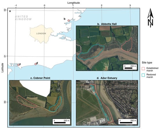
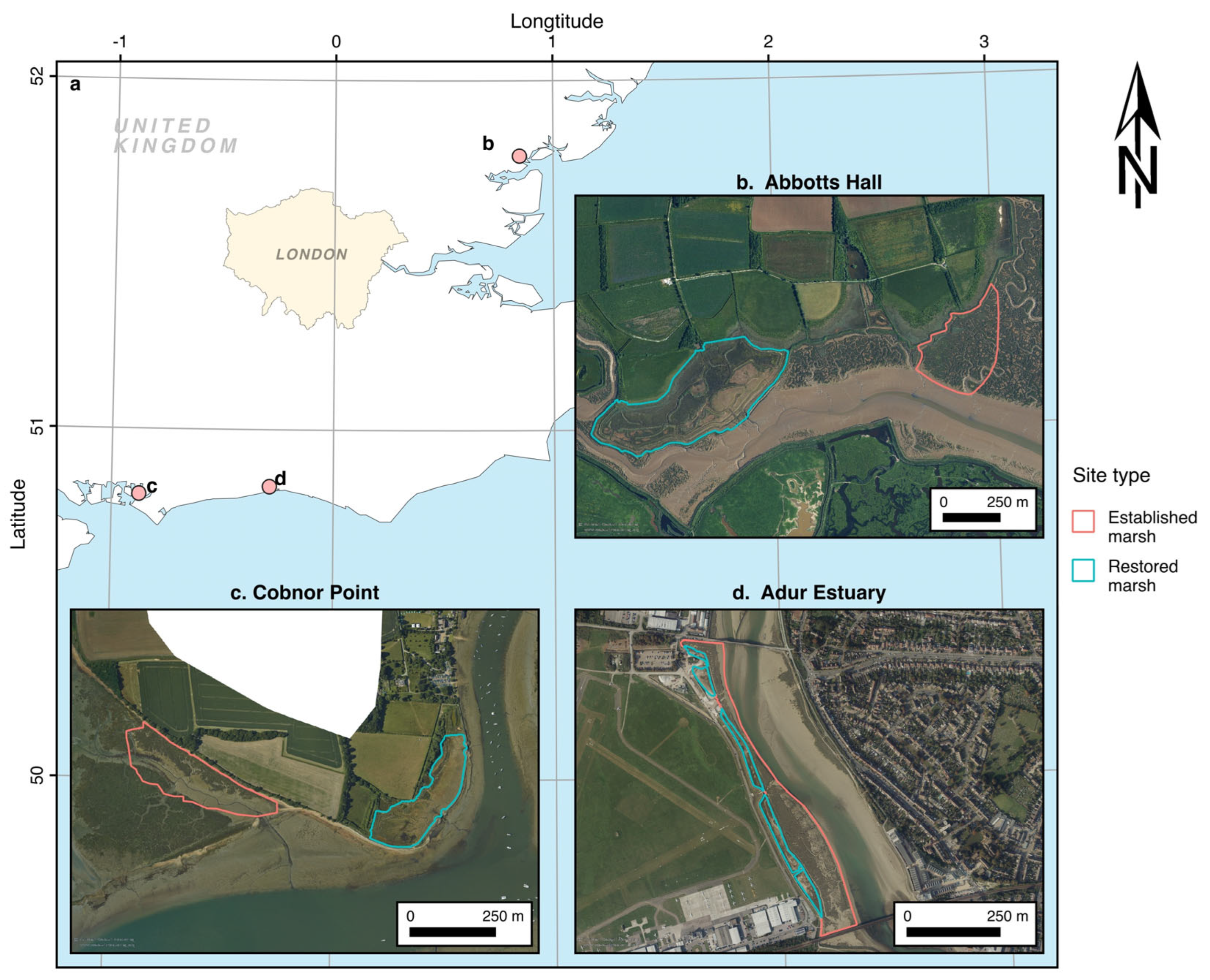
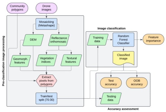
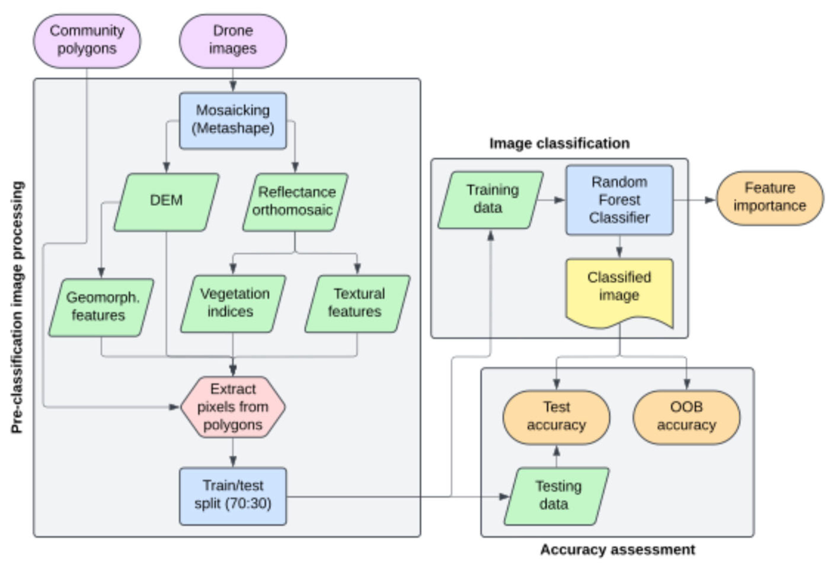
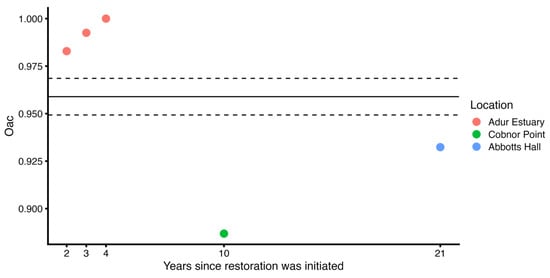
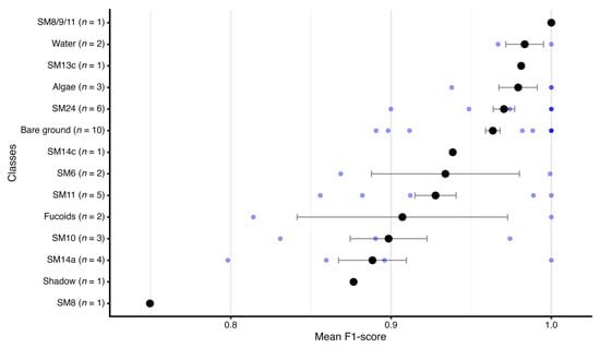
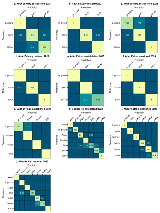
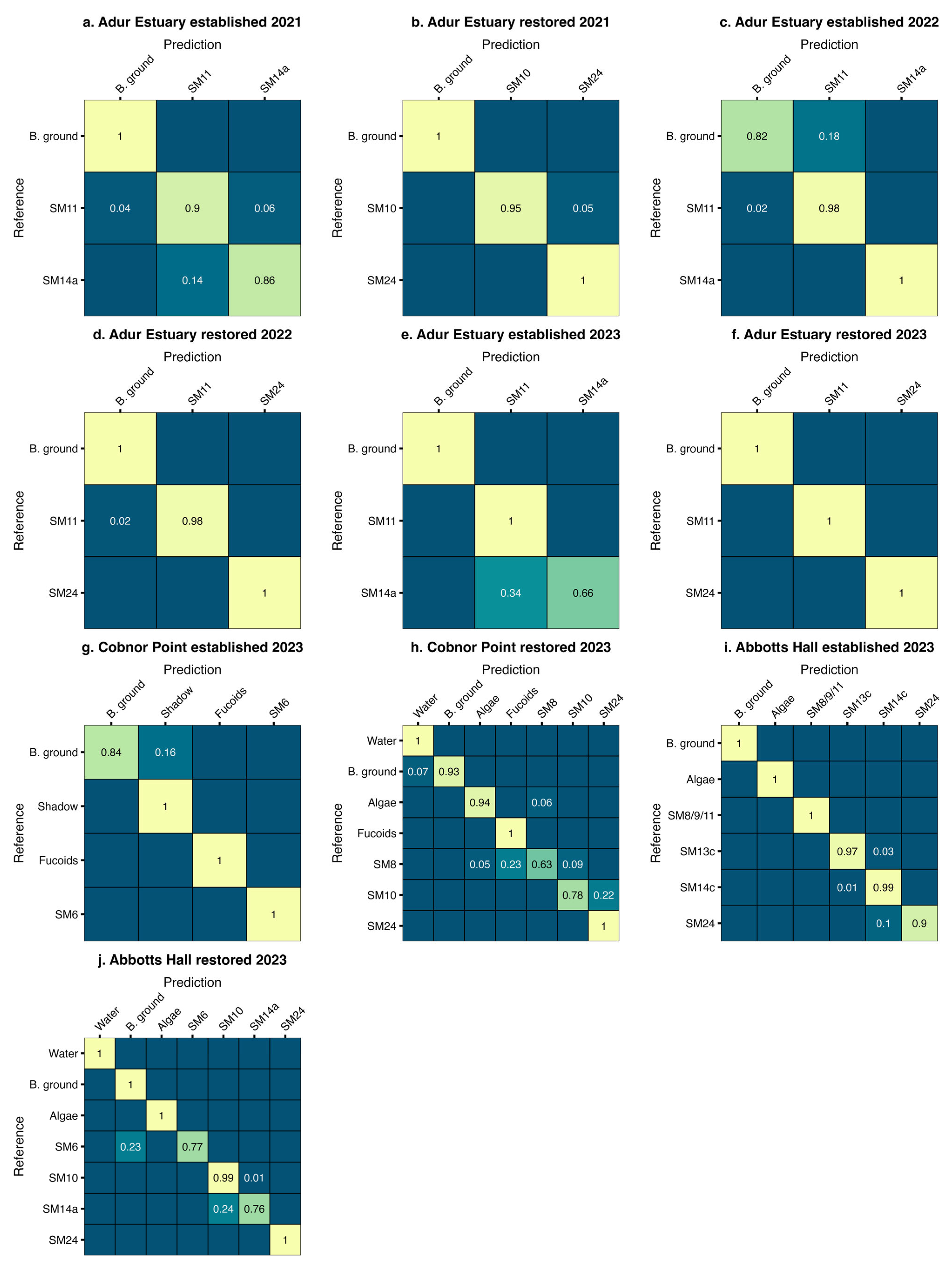
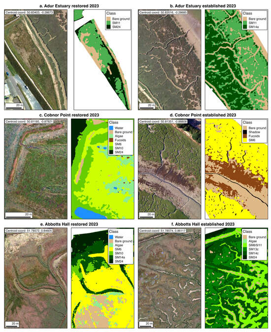
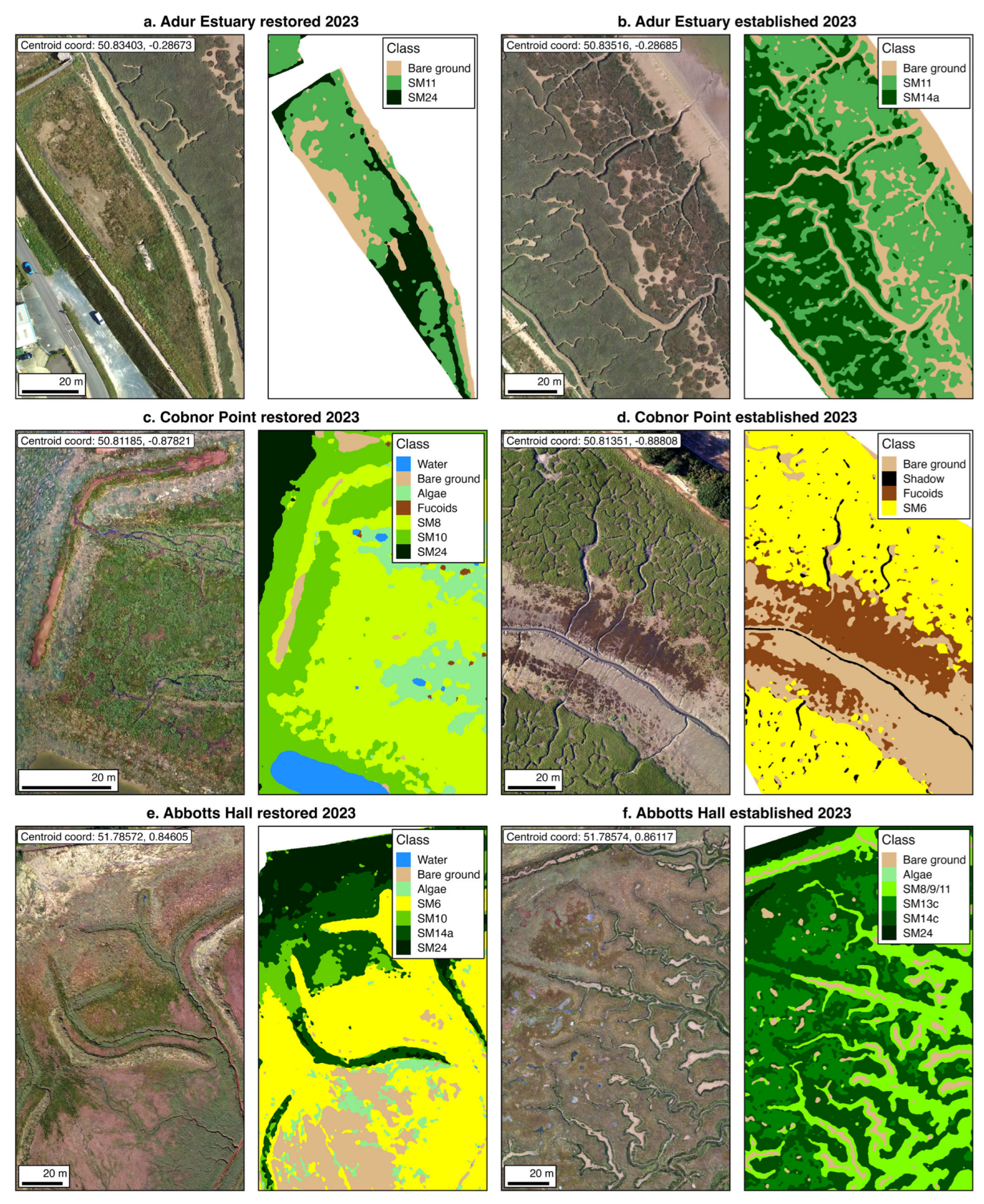
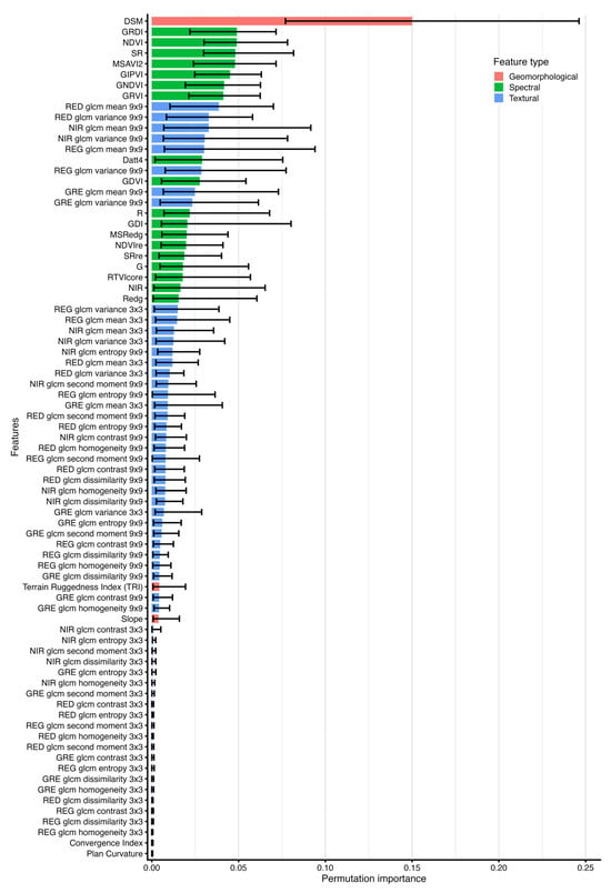

Disclaimer/Publisher’s Note: The statements, opinions and data contained in all publications are solely those of the individual author(s) and contributor(s) and not of MDPI and/or the editor(s). MDPI and/or the editor(s) disclaim responsibility for any injury to people or property resulting from any ideas, methods, instructions or products referred to in the content. |
© 2026 by the authors. Licensee MDPI, Basel, Switzerland. This article is an open access article distributed under the terms and conditions of the Creative Commons Attribution (CC BY) license.