Statistical Assessment of Accuracy and Precision in Satellite Spatial Quality Measurement Using Natural Edge Targets from KOMPSAT-3A

Highlights

What are the main findings?

• Optical satellite spatial quality measurements (RER, HFWHM, MTF50, and MTFA) using Natural edge targets.
• Statistical quantitative accuracy and precision of them.

What are the implications of the main findings?

• Natural edge targets can effectively replace ground-based artificial edge targets.
• Accurate spatial quality measurement in one day.

Abstract

The spatial quality (RER, FWHM, MTF50, and MTFA) of an on-orbit high-resolution Earth observation satellite was statistically assessed using edges extracted from natural targets in urban imagery, rather than from a ground-based artificial edge target (Edge target). A total of 8414 edge patches were automatically extracted from Natural Targets (NT) in 24 images acquired over 11 cities worldwide by KOMPSAT-3A. The spatial quality results derived from NT edges were compared with those obtained from an Edge target in terms of accuracy and precision. The averaged spatial quality values were nearly identical between the two approaches. However, the coefficient of variation (CV), used to quantify precision, was approximately two times higher for NT edges. Despite this lower precision, NT-based assessment provides substantial operational advantages. While 549 Edge target acquisitions over eight years yielded only 1098 usable edge images, a single acquisition over Las Vegas produced 366 NT edge images. These findings indicate that statistically reliable spatial quality estimates with comparable accuracy can be achieved within a single day using abundant NT edges, without the need to construct and maintain dedicated Edge targets.

1. Introduction

To evaluate the spatial quality of high-resolution Earth observation satellites operating in orbit, the most widely adopted method is to compute spatial quality estimators from edge images acquired over ground-based artificial edge targets (hereinafter Edge target) [1,2,3,4,5,6,7,8,9,10,11,12,13,14,15,16]. For satellites capable of stellar imaging, spatial quality estimators—excluding RER (Relative Edge Response on ESF; Edge Spread Function)—such as FWHM (Full Width at Half Maximum on LSF; Line Spread Function) and MTF50 (MTF value at Nyquist frequency on MTF curve) can also be derived from star images [12,13,14,15,16,17,18,19]. In addition, medium- and low-resolution satellites, such as Landsat and NOAA satellites, have been evaluated using edge images extracted from lunar observations [20,21]. For certain high-resolution optical satellites where edge extraction from dedicated Edge targets is challenging, spatial quality has been assessed using a limited number of natural edge targets acquired from real scenes [22,23,24,25]. Some studies have further examined the applicability and reliability of spatial quality measurements derived from natural targets [25,26,27,28]. However, although different satellites were investigated in these studies, most of them analyzed only one or two natural edge targets, and at most approximately ten edges. Consequently, none of these works reported quantitative precision metrics due to the limited sample size.

Natural targets such as stars, the Moon, bridges, and terrain features generally exhibit lower reliability and are applicable only under specific conditions; therefore, they are not widely used in routine spatial quality assessment. Consequently, CEOS WGCV IVOS (Committee on Earth Observation Satellites, Working Group on Calibration and Validation, Infrared Visible Optical Sensors subgroup) and USGS EROS (U.S. Geological Survey’s Earth Observation and Science center) share information on Edge targets worldwide for public use [29,30], and ESA ESRIN (European Space Agency, European Space Research Institute) is planning to construct edge targets within the Cal/Val Park of the Earthnet Data Assessment Project (EDAP) [31]. When properly maintained, Edge target provide very high accuracy and precision; however, they suffer from several critical limitations in operational use. First, they are applicable only to high-resolution satellites. Second, due to satellite ground track constraints and weather conditions, a single edge target can typically be imaged only about once per week. Third, edge targets require significant construction costs as well as regular maintenance. Fourth, spatial quality estimates derived from only two edge images extracted from a single edge target acquisition exhibit statistically low precision. Fifth, for satellites operating in descending orbits, there are no edge targets that can be imaged within the allowable edge angle range when the targets are constructed to match ascending orbits. Sixth, as of 2025, only four operational edge targets are available worldwide, located in Baotou (China), India, Salon (France), and Zuunmod (Mongolia) [1].

This paper presents spatial quality measurement results derived from natural target (NT) edges extracted from urban imagery (hereinafter NT edge) and statistically verifies that they can achieve accuracy comparable to that obtained using Edge targets, while overcoming the aforementioned limitations. High-resolution satellites such as KOMPSAT-3A can extract a sufficient number of NT edges from urban scenes, and even for medium- and low-resolution satellites, statistically meaningful spatial quality assessment becomes feasible if a sufficient number of edges can be extracted from natural targets.

In this study, only across NT edges extracted from urban imagery were used for spatial quality assessment. Along-track spatial quality was not considered because, due to the Time Delay Integration (TDI) CCD characteristics of KOMPSAT-3A, the along-track measurements incorporate additional line-rate prediction effects. As a result, along-track spatial quality values are generally lower and exhibit reduced measurement precision compared to across results. Only the across spatial quality values are officially defined and specified for KOMPSAT-3A [1]. Furthermore, only Level 0 data (raw image data) were used in this study. The use of Level 0 imagery ensures that the intrinsic spatial performance of the satellite system is evaluated without influence from any ground-based image processing. The official spatial quality requirement for KOMPSAT-3A (MTF50 > 8%) is also defined based on Level 0 data.

The accuracy and precision of spatial quality measurements derived from NT edges extracted from urban imagery are evaluated and verified using statistical methods. As a reference dataset, this study uses the mean spatial quality values obtained from 31,127 across edges that satisfied the Edge target Spatial quality Measurement Python code (hereinafter ESMP) constraints [1], extracted from a total of 36,425 across edges. These edges were derived by fixing the ‘number of edge row line’ (hereinafter EdgeLine) to 21 pixels (EdgeLine = 21 pixels) from 1098 across edge images acquired during 549 edge target observations conducted by KOMPSAT-3A over the Baotou, India, Salon, and Zuunmod edge targets between 19 January 2017 and 3 March 2025. For precision comparison, the coefficient of variation (hereinafter CV), defined as the ratio of the standard deviation to the mean, which is widely used in statistics, is computed and compared [32].

For spatial quality estimation from NT edges, the ESMP developed by KARI [1,2] was directly applied. Only the NT edge detection and extraction procedure, as well as the statistical aggregation of ESMP-derived spatial quality estimators, was newly implemented in ‘NT_edge.py’ Python version 3.14 code [33].

To date, the spatial quality assessment of on-orbit Earth observation satellites has typically relied on a limited number of acquisitions over Edge targets. In this context, the contributions of this paper are summarized as follows:

• This paper demonstrates, through statistical analysis, that mean spatial quality estimates derived from NT edges extracted from urban imagery can achieve accuracy comparable to that obtained using Edge targets.
• Although the measurement precision of spatial quality estimates derived from NT edges is approximately a factor of two lower than that obtained from Edge targets, this level of degradation is shown to be consistent with expectations given the inherent characteristics of natural targets.
• The results indicate that a statistically reliable estimation of spatial quality can be achieved within a single day using a large number of NT edges, whereas Edge targets may not be observable or may provide an insufficient number of images to ensure reliable precision within the same time frame.

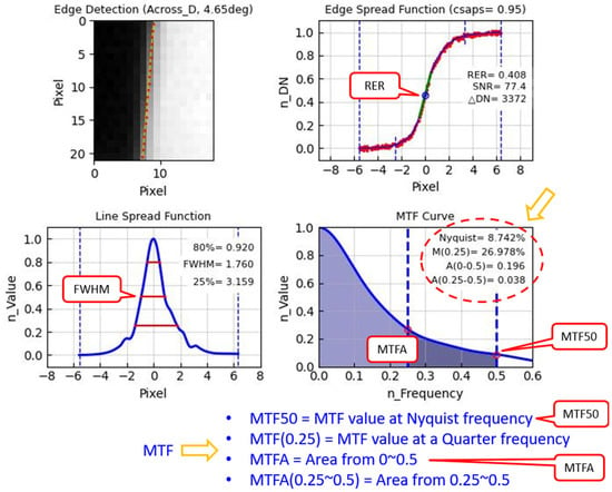
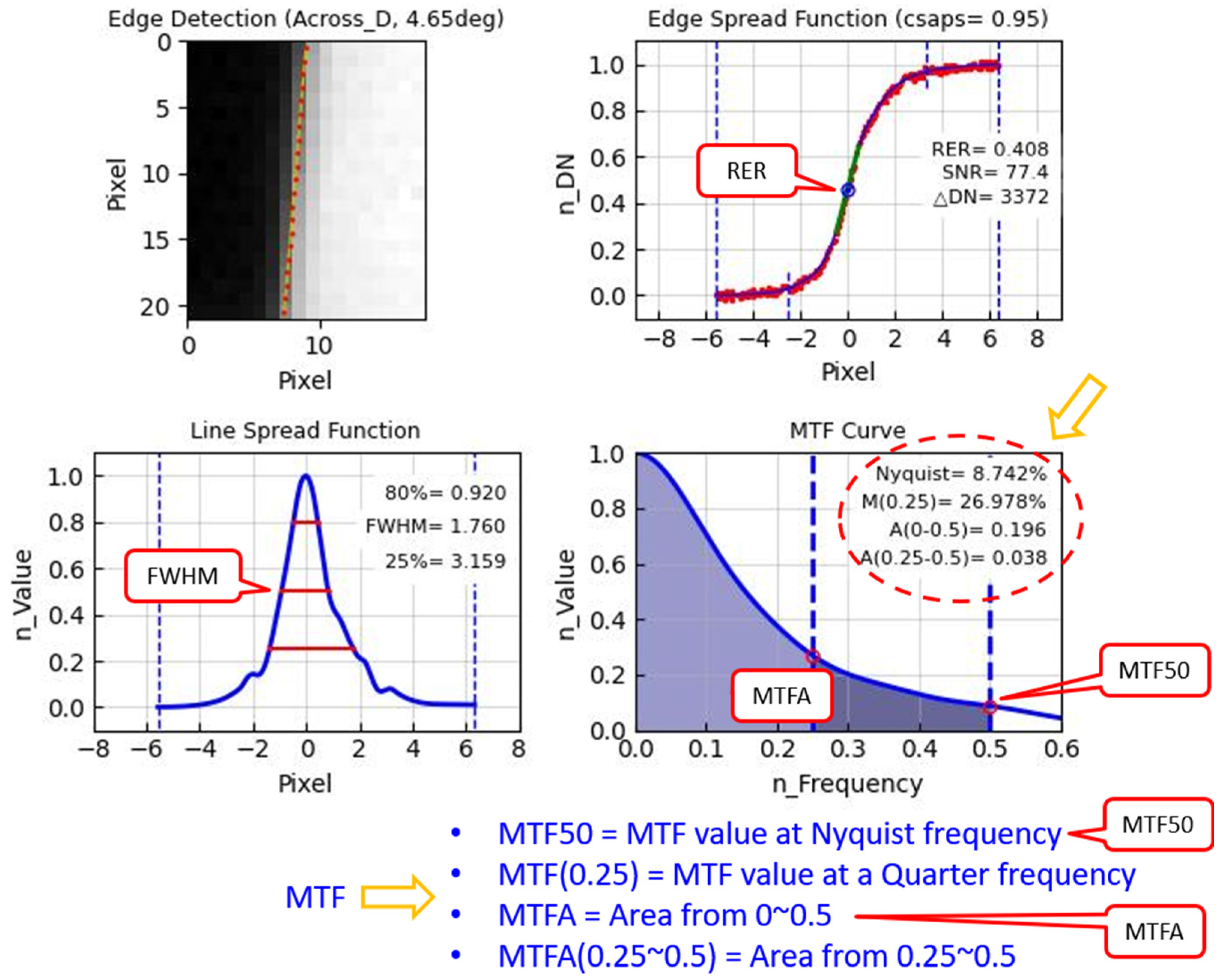
Figure 1 presents an example of ESMP result plots and illustrates the measurement locations and definitions of the spatial quality estimators (RER, FWHM, MTF50 and MTFA; MTF Area on MTF curve) [1].

Figure 1. Plot showing the procedure of using the Edge target to measure the spatial quality (RER, FWHM, MTF50, MTFA) using KOMPSAT-3A Level 0 (raw) across Edge image data imaged at Zuunmod with a roll tilt of 29.31 degrees on 21 February 2019.

Section 2 describes the procedure for computing spatial quality estimators from NT edges, Section 3 summarizes the global cities imaged by KOMPSAT-3A for NT edge extraction, Section 4 compares spatial quality results derived from Edge targets and NT edges, and Section 5 concludes the paper and outlines directions for future work.

2. NT Edge Extraction and Spatial Quality Measurement Procedure

2.1. Improvements to ESMP

The ESMP used in this study is an updated version of the previously reported ESMP [1], incorporating improvements in ESF fitting precision [34,35]. In the original implementation, noise in the ESF was suppressed using a first cubic smoothing approximation spline (hereinafter CSAPS fitting, followed by a second CSAPS fitting to obtain the final fitted ESF. In the updated ESMP, a Savitzky–Golay filter (hereinafter SGolay) is first applied, and noise exceeding the 2σ threshold is removed prior to spline fitting. Subsequently, a first CSAPS fitting is performed, followed by a second CSAPS fitting to obtain the final fitted ESF. The introduction of the initial SGolay step improves edge preservation compared to CSAPS alone and reduces the correlation between EdgeLine length and the resulting spatial quality estimators, which can otherwise arise from ESF fitting sensitivity [33,36]. It should be noted that parametric fitting methods were not adopted. Instead, non-parametric approaches (CSAPS and SGolay) were employed because the ESF of satellite optical systems typically exhibits asymmetry, making parametric modeling unsuitable [1,37].

Table 1 presents a comparison of the mean spatial quality values and CV statistics before and after the application of SGolay filtering, using edge images acquired over Edge targets imaged by KOMPSAT-3A [34]. The improved ESMP employed in this study demonstrates slightly improved spatial quality measurement performance compared to the previous version.

Table 1. Comparison of mean spatial quality estimates and CV before and after application of the SGolay filter using KOMPSAT-3A Edge target imagery.

		RER	FWHM	MTF50	MTFA
Dual CSAPS	Mean	0.393	1.857	9.520	0.413
	CV	0.0355	0.0525	0.1573	0.0514
SGolay Dual CSAPS	Mean	0.395	1.839	9.866	0.415
	CV	0.0350	0.0515	0.1617	0.0544

2.2. Spatial Quality Measurement Procedure Using NT Edge

Table 2 provides a brief description of the structure and computational workflow of the additional Python code developed to measure spatial quality from NT edges extracted from urban imagery. The overall process of extracting NT edges from urban images and storing the final results is implemented using the NT_edge.py in conjunction with ESMP.

Table 2. Workflow to obtain the spatial quality in KARI’s Python code.

	Edge Target	NT Edge	Python Code	Estimator
1	Full & EdgeLine = 21 pixel	Searching edge by EdgeLine = 21 pixel	(NT) NT_edge.py
2	Across edge (2) Along edge (2)	Across & Along	(Edge) ESMP (NT) NT_edge.py
3	ESF		ESMP	RER
4	LSF			FWHM
5	MTF curve			MTF50, MTFA
6	Constraint & IQR
7	Statistics (Across & Along)	Statistics (Across & Along per city)
8	Save results		(Edge) ESMP (NT) NT_edge.py

As NT_edge.py extracts all NT edges from the urban imagery, it calls ESMP to process each extracted edge. ESMP first classifies the NT edge into across and along directions and then computes the spatial quality estimators (RER, FWHM, MTF50 and MTFA). For each imaged city, ESMP stores the corresponding statistical results after applying predefined constraints and the interquartile range (IQR) outlier exclusion method, defined as Q1 − 1.5 × IQR to Q3 + 1.5 × IQR (hereinafter IQR) [1].

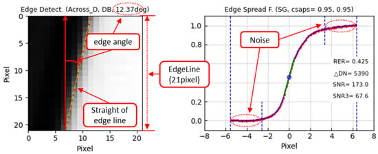
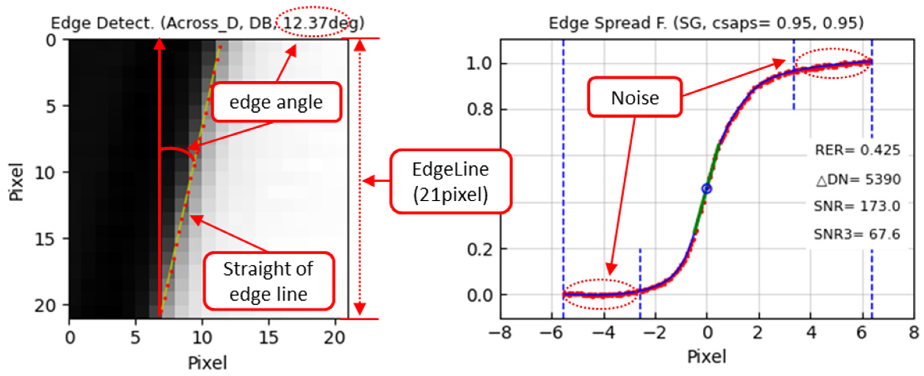
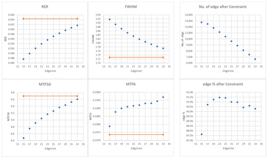
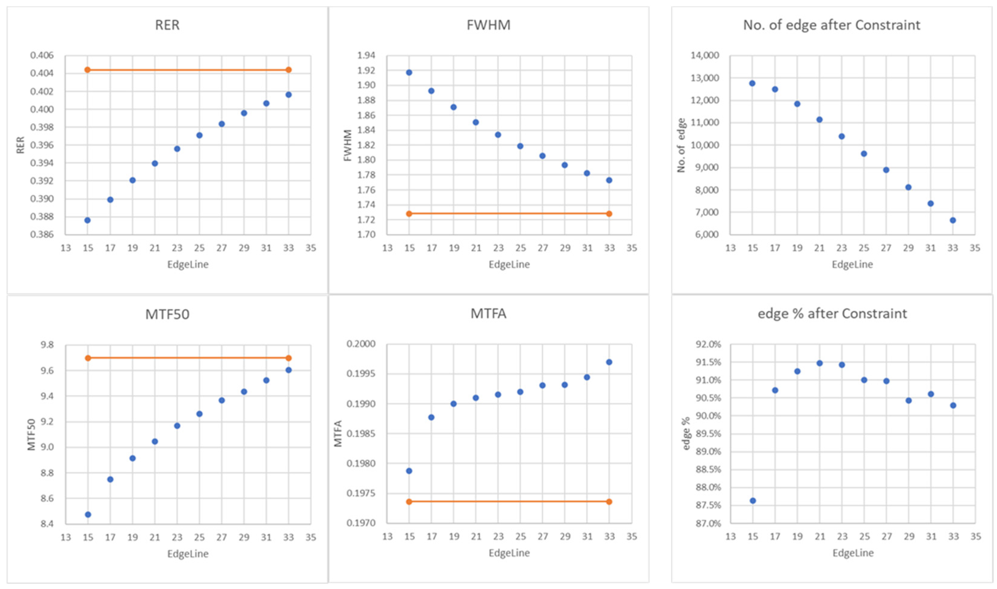
As shown in Figure 2, NT edges were extracted using a fixed EdgeLine of 21 pixels, while the ESMP processes artificial edge targets using both the full edge extent and a truncated EdgeLine 21 pixels configuration, storing the corresponding spatial quality results in separate output files [1]. As illustrated in Figure 3, the spatial quality estimators exhibit a proportional relationship with EdgeLine due to the characteristics of the SGolay and CSAPS fitting applied during the ESF fitting process. The measurements converge at approximately 40 pixels (indicated by the orange horizontal line in Figure 3). In the upper-right plot of Figure 3, the number of NT edges satisfying the ESMP constraints shows a steep inverse relationship with EdgeLine. In practice, securing NT edges with EdgeLine = 40 pixels is extremely difficult in natural scenes. To ensure a statistically sufficient number of edge images, EdgeLine = 21 pixels was selected, as it provides the highest retention ratio of valid NT edges after applying all constraints (see the lower-right plot of Figure 3) [1,4,33,36]. Although it is theoretically possible to construct a look-up table to compensate for the difference between EdgeLine = 21 pixels and the 40-pixel convergence point, such a correction would require additional comprehensive analysis to establish statistically reliable adjustment factors. Therefore, this compensation was not incorporated in the present study.

Figure 2. Description of the four edge selection criteria applied in ESMP: edge straightness, edge angle, noise level, and number of edge row line (EdgeLine).

Figure 3. Relationship between EdgeLine and spatial quality estimators. The orange line denotes the full-edge result from the Edge target. The right column shows the number and retention ratio of edges after applying ESMP constraints. Although convergence occurs at ~40 pixels, EdgeLine = 21 pixels was selected to secure sufficient edge images [1,4,33,36].

2.3. NT Edge Extraction Process and Edge Conditions

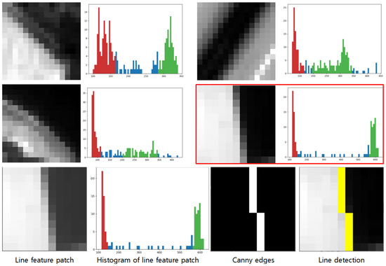
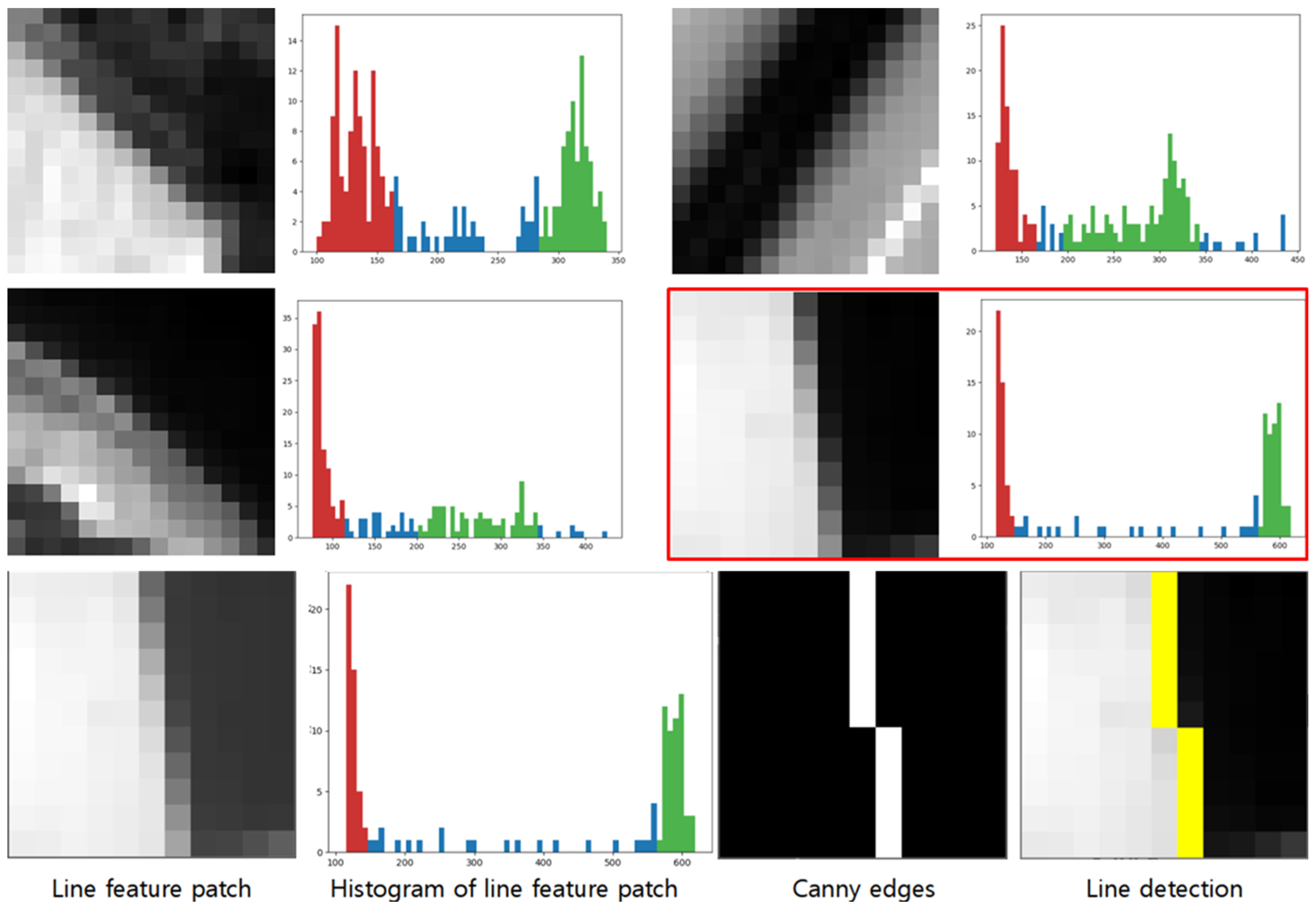
Figure 4 illustrates the procedure for identifying NT edge candidates from natural targets in urban imagery.

Figure 4. Workflow for final NT edge selection from urban imagery: NT edge candidates identified using mean shift clustering (red box in the second row) [38] are refined using Canny edge detection and the Hough transform [39]. In the histogram plot, red and green are dark and bright areas, respectively, and the yellow area in ‘Line detection’ plot is the detected edge.

The NT_edge.py identifies NT edge candidates from urban imagery using the Mean Shift clustering method [38,39]. The procedure is summarized as follows:

①

Based on the EdgeLine = 21 pixels condition, a 21 × 21 pixel window is moved across the urban image with a 5-pixel stride, and a histogram is computed for each patch.

②

For each histogram, the presence of two clusters is examined, each containing at least one-third of the total pixels. In addition, the difference between the mean pixel values of the two clusters must exceed 2048. (Among the examples in Figure 4, only the second red box in the second row satisfies this condition.)

③

For the qualified patches, Canny edge detection is applied, followed by Hough transform-based line detection to obtain the final NT edge candidates (Figure 4, third row).

Most of the selected NT edge candidates are subsequently rejected by four edge-related constraints among the ten ESMP constraints [1] (Figure 2; Table 3). In particular, the straightness of the detected edge line and the CV of noise are approximately 1.3 times worse for NT edges than for artificial edge targets. This discrepancy directly explains the reduced retention ratio of usable NT edges after constraint filtering (Table 5).

Table 3. Edge conditions and constraint values used in this study.

Constraint Condition	Description	Constraint Value in ESMP
edge straightness	Linear fitting error of the edge fitting results (red circles) for all edge row lines in the upper-left image of Figure 1	≤0.1 pixel
edge angle tolerance	Angle between the line of the edge and the satellite flight direction (y-direction in the upper-left image of Figure 1)	≥2.2 deg & ≤30 deg
noise	ESF fitting error in the ESF plot shown in the upper-right panel of Figure 1	noise @ dark area ≤ 0.045 noise @ bright area ≤ 0.05
EdgeLine	Total number of edge row lines used for ESF computation in the upper-left image of Figure 1	=21 pixel

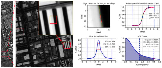
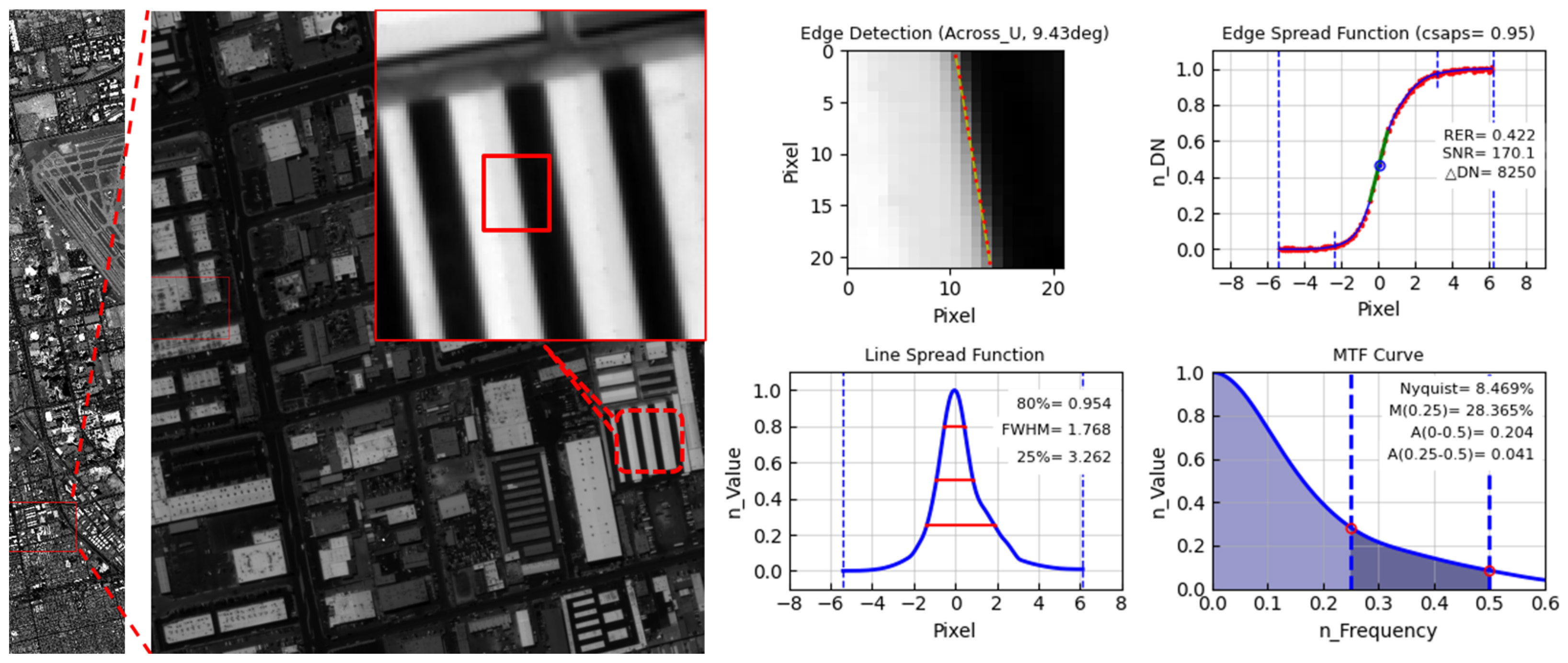
Figure 5 presents an example of spatial quality measurement for one of the 316 across NT edges automatically extracted using NT_edge.py from KOMPSAT-3A imagery acquired over Las Vegas on 2 March 2021.

Figure 5. Example of spatial quality measurement from an across NT edge, one of the 316 NT edges automatically extracted from KOMPSAT-3A imagery acquired over Las Vegas on 2 March 2021. The red box on the left image is an edge candidate, and the plot on the right is the spatial quality measurement result.

3. Cities Imaged by KOMPSAT-3A and NT Edges

Among more than 50 urban images globally acquired by KOMPSAT-3A between 2014 and 2018, 24 images from 11 cities were selected for this study. To secure a sufficient number of NT edges satisfying the EdgeLine = 21 pixels criterion within a single image, cities were preferentially selected from the acquisition archive based on the following characteristics: large building footprints, relatively low building heights, and urban populations exceeding 500,000. As a result, many suitable images were identified from cities located in the western United States, Australia, and South Africa. In contrast, cities in Europe, South America, and Asia were excluded because their urban morphology—characterized by smaller building footprints and a higher proportion of high-rise structures—typically yielded only approximately ten NT edges per image satisfying the EdgeLine = 21 pixels condition. This limited edge image size was considered insufficient to ensure statistically reliable analysis.

Table 4 summarizes the acquisition dates and roll tilt angles for the urban imagery, the total number of detected across NT edges, the number of across NT edges remaining after applying the ESMP constraints (const.), and the mean spatial quality values (RER, FWHM, MTF50 and MTFA) with the corresponding CV values after additionally applying the IQR-based outlier exclusion method. For reference, a total of 12,122 along NT edges were initially detected, of which 8060 remained after the application of the constraints.

Table 4. List of 24 KOMPSAT-3A images acquired over 11 cities, including acquisition dates and roll tilt angles, the total number of detected NT edges, the number of across NT edges after applying constraints (const.), and the city-wise mean spatial quality values (RER, FWHM, MTF50, MTFA) with CV values after applying the IQR-based outlier exclusion method.

Date	City	Roll	No. of Edges			RER	FWHM	MTF50	MTFA
			Total	Const.	%
22 June 2018	Pretoria	1.51	233	171	73.4	0.398 (0.068)	1.865 (0.083)	8.806 (0.262)	0.413 (0.081)
2 January 2019	Las Vegas	−8.23	366	249	68.0	0.380 (0.060)	1.963 (0.070)	8.737 (0.252)	0.399 (0.066)
25 February 2019	Las Vegas	−16.50	475	272	57.3	0.388 (0.051)	1.889 (0.061)	9.540 (0.271)	0.417 (0.083)
1 November 2019	Tucson	15.16	43	28	65.1	0.400 (0.079)	1.946 (0.100)	7.777 (0.326)	0.407 (0.090)
16 November 2019	Houston	8.00	231	163	70.6	0.405 (0.055)	1.834 (0.082)	9.654 (0.275)	0.425 (0.080)
14 December 2019	LA	2.48	107	68	63.6	0.400 (0.101)	1.879 (0.096)	8.859 (0.323)	0.414 (0.085)
4 March 2020	San Diego	−25.59	187	117	62.6	0.390 (0.070)	1.875 (0.079)	9.116 (0.261)	0.415 (0.083)
18 September 2020	Denver	10.98	183	128	69.9	0.404 (0.078)	1.848 (0.078)	9.222 (0.273)	0.416 (0.089)
21 September 2020	Dallas	−5.45	821	559	68.1	0.390 (0.083)	1.882 (0.084)	9.386 (0.271)	0.411 (0.087)
2 March 2021	Las Vegas	1.78	316	242	76.6	0.394 (0.070)	1.923 (0.068)	9.334 (0.220)	0.422 (0.075)
11 March 2021	Phoenix	17.53	1210	790	65.3	0.418 (0.086)	1.768 (0.091)	12.134 (0.301)	0.448 (0.086)
8 September 2021	Denver	−1.44	399	286	71.7	0.396 (0.076)	1.876 (0.068)	9.104 (0.247)	0.416 (0.087)
3 November 2021	LA	17.81	35	25	71.4	0.420 (0.069)	1.880 (0.084)	9.091 (0.426)	0.421 (0.136)
4 November 2021	LA	−7.66	309	233	75.4	0.391 (0.062)	1.861 (0.072)	9.526 (0.259)	0.408 (0.079)
7 December 2021	Dallas	11.18	311	214	68.8	0.399 (0.083)	1.869 (0.103)	9.302 (0.386)	0.424 (0.111)
26 February 2022	LA	5.92	72	47	65.3	0.396 (0.081)	1.829 (0.103)	10.667 (0.300)	0.442 (0.109)
17 March 2022	San Jose	−24.74	316	163	51.6	0.381 (0.076)	1.956 (0.089)	7.925 (0.276)	0.405 (0.081)
25 March 2022	LA	18.32	149	102	68.5	0.408 (0.097)	1.851 (0.118)	10.491 (0.300)	0.426 (0.099)
11 July 2022	LA	−8.95	296	202	68.2	0.388 (0.077)	1.902 (0.084)	9.559 (0.310)	0.416 (0.092)
17 May 2023	Salt Lake	−16.05	1629	1102	67.6	0.377 (0.073)	1.849 (0.067)	9.756 (0.292)	0.426 (0.106)
23 February 2024	Phoenix	24.58	257	108	42.0	0.406 (0.068)	1.853 (0.090)	10.349 (0.268)	0.428 (0.082)
15 April 2024	Las Vegas	22.01	68	41	60.3	0.423 (0.069)	1.773 (0.081)	11.119 (0.248)	0.441 (0.096)
27 May 2024	Denver	8.67	221	110	49.8	0.393 (0.082)	1.935 (0.114)	10.163 (0.404)	0.436 (0.114)
1 August 2024	Dallas	8.88	180	111	61.7	0.417 (0.097)	1.822 (0.083)	9.735 (0.313)	0.431 (0.099)
	Total		8414	5531	65.7	0.394 (0.083)	1.860 (0.084)	9.817 (0.304)	0.423 (0.097)

KOMPSAT-3A has a ground sampling distance (GSD) at nadir of 55 cm, an MTF value at the Nyquist frequency (MTF50) exceeding 8% for Level 0 imagery, and a swath width at nadir of 15 km. In this study, only KOMPSAT-3A Level 0 images were used. NT edges were searched across the full image swath, and only across NT edges were employed for the analysis. Among the analyzed scenes, the Salt Lake City image acquired on 17 May 2023 contains the largest number of NT edges, whereas the images acquired over Tucson (1 November 2019), Los Angeles (14 December 2019, 3 November 2021 and 26 February 2022), and Las Vegas (15 April 2024) contain the smallest numbers. A comparison among the four Las Vegas acquisitions, six Los Angeles acquisitions, and three Dallas acquisitions shows that the number of detected NT edges varies significantly depending on the imaged urban area within the KOMPSAT-3A swath width of approximately 15 km.

4. Results and Discussion

This section is divided into two main parts. First, the characteristics and biases of the spatial quality measurement results derived from NT edges extracted from KOMPSAT-3A imagery are described. Second, representative spatial quality estimators (RER, FWHM, MTF50, MTFA) obtained from NT edges are compared and analyzed, with an emphasis on the precision of each estimator.

4.1. Characteristics and Biases of Spatial Quality Measurements from NT Edges

This subsection summarizes the statistical results of spatial quality measurements derived from 5531 NT edges extracted from 24 urban images acquired by KOMPSAT-3A between 2018 and 2024. Table 5 presents the mean spatial quality values, CV, skewness, and kurtosis for three cases: Edge targets using full EdgeLine, Edge targets with EdgeLine = 21 pixels, and NT edges. For the 957 full-edge cases extracted from Edge targets, the mean EdgeLine is 49 pixels, with a maximum of 102 pixels and a minimum of 26 pixels. As discussed in Section 2.3, a proportional relationship exists between EdgeLine and the spatial quality measurement values [1,4,33,36]. Consequently, the mean spatial quality values obtained from full EdgeLine cases are better than those derived from Edge targets with EdgeLine = 21 pixels.

Table 5. Mean spatial quality values (accuracy), CV (precision), skewness, and kurtosis for Edge targets using full EdgeLine, Edge targets with EdgeLine = 21 pixels, NT edges, and NT edges excluding the Phoenix (11 March 2021) dataset. The numbers in parentheses in the second column indicate the number of edges remaining after applying constraints, the total number of detected edges, and the corresponding ratio.

Target			RER	FWHM	MTF50	MTFA
Edge target	Full edge (957/1098/87.2%)	Mean	0.407	1.727	10.142	0.411
		CV	0.032	0.045	0.134	0.045
		Skew	0.054	0.050	0.236	0.210
		Kurt.	−0.217	−0.104	−0.060	−0.175
	EdgeLine = 21 (31,127/36,425/85.5%)	Mean	0.395	1.855	9.284	0.408
		CV	0.036	0.051	0.184	0.061
		Skew	0.052	0.075	0.278	0.167
		Kurt.	−0.185	−0.197	−0.104	−0.093
NT edge	EdgeLine = 21 (5531/8181/67.6%)	Mean	0.394	1.860	9.817	0.423
		CV	0.083	0.084	0.304	0.097
		Skew	0.170	0.203	0.509	0.360
		Kurt.	−0.172	−0.018	−0.120	−0.261
	Except Phoenix (11 March 2021) (4741/6971/68.0%)	Mean	0.390	1.874	9.413	0.418
		CV	0.078	0.081	0.288	0.093
		Skew	0.099	0.306	0.427	0.376
		Kurt.	−0.175	−0.065	−0.66	−0.232

A comparison of the city-wise mean spatial quality values listed in Table 4 shows that the spatial quality measurements for Phoenix (11 March 2021), which contains 790 NT edges, are relatively higher than the overall mean values. The underlying cause of this discrepancy requires further comprehensive investigation, considering multiple factors such as the acquisition command parameters at the imaging time, the satellite and camera status data, and the geographic imaging conditions of KOMPSAT-3A. The last row of Table 5 presents the averaged spatial quality estimators excluding the Phoenix (11 March 2021) scene. Compared to the Edge target (EdgeLine = 21 pixels), the differences in RER and FWHM slightly increased, whereas MTF50 and MTFA became closer to the reference values. These results suggest that the inclusion of the Phoenix scene influences the overall statistical comparison, particularly for MTF-based estimators.

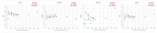
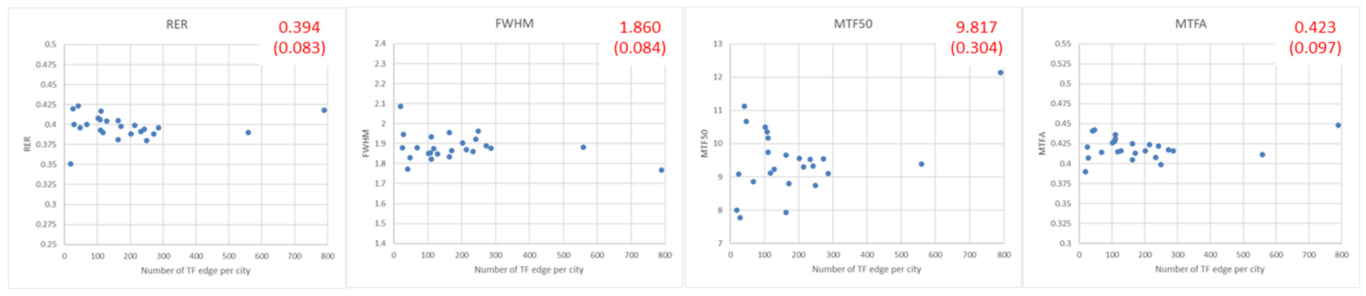
Second, a commonly used empirical rule of thumb in statistics suggests that a minimum sample size of approximately 30~50 is required for reliable estimation [40]. As shown in Figure 6, the mean spatial quality values exhibit a tendency to converge as the number of NT edges per city increases. Although the number of analyzed cities is still limited and Figure 6 alone is insufficient to definitively determine the minimum required number of NT edges per city, a conservative threshold of approximately 100 NT edges is tentatively adopted in this study. As additional urban imagery becomes available in future work, a more robust determination of the minimum number of NT edges required for statistically reliable city-wise mean spatial quality estimation will be pursued.

Figure 6. Relationship between the number of NT edges per city and the mean spatial quality values (RER, FWHM, MTF50, MTFA). The mean spatial quality values tend to converge when the number of NT edges reaches approximately 100. The rightmost data point in each plot corresponds to the Phoenix (11 March 2021) dataset, which contains 790 NT edges. Red numbers indicate mean values, and the numbers in parentheses represent the corresponding CV.

According to the results in Table 5, the mean spatial quality values derived from NT edges and those obtained from Edge targets with EdgeLine = 21 pixels are comparable in the spatial domain, as reflected by RER and FWHM. In the frequency domain, however, the MTF50 and MTFA values derived from NT edges are higher than those obtained from edge targets. In contrast, the measurement precision, quantified by the CV, is approximately a factor of two worse for NT edges compared to edge targets with EdgeLine = 21 pixels. Considering these results together with the fact that the proportion of edges remaining after constraint application is more than two times lower for NT edges, it is conjectured that NT edges contain relatively stronger high-frequency noise components. This increased noise likely leads to higher frequency-domain estimators (MTF50 and MTFA) as well as larger CV values. Nevertheless, further detailed analysis is required to confirm this hypothesis [41,42,43,44]. In particular, the underlying reasons for the consistently larger MTFA values observed for NT edges warrant additional investigation based on a more fundamental analysis of the measurement process.

4.2. Comparative Analysis of NT Edge’s Spatial Quality Estimators’ Results

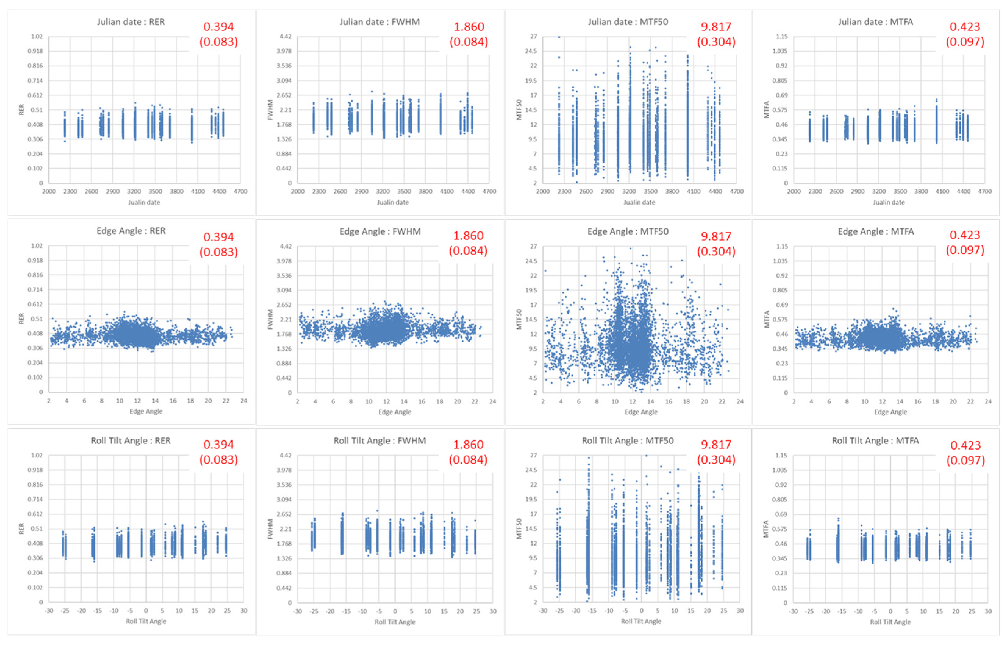
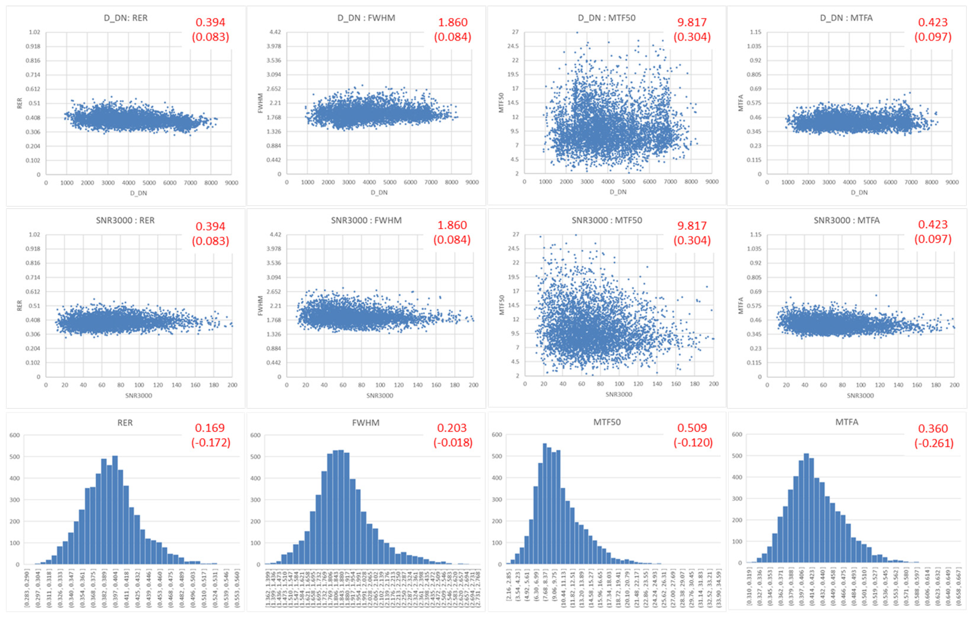
Figure 7 and Figure 8 present the characteristics and biases of the spatial quality measurements (RER, FWHM, MTF50, MTFA) derived from across NT edges. The results are analyzed with respect to the following factors, and the y-axis scales for RER, FWHM, MTF50, and MTFA are individually adjusted according to their respective CV values:

Figure 7. (top) Julian date versus RER, FWHM, MTF50, and MTFA; (middle) edge angle; and (bottom) roll tilt angle. Red numbers indicate mean values, and the numbers in parentheses represent the corresponding CV. The y-axis scale for each estimator is adjusted according to its CV value.

Figure 8. (top) ΔDN versus RER, FWHM, MTF50, and MTFA; (middle) SNR versus RER, FWHM, MTF50, and MTFA. Red numbers indicate mean values, and the numbers in parentheses represent the corresponding CV. The y-axis scale for each estimator is adjusted according to its CV value. (bottom) Histograms are used to examine the z-distributions, where red numbers indicate skewness values and the numbers in parentheses represent kurtosis values.

• Julian date (since 17 May 2012, the launch date of KOMPSAT-3);
• Edge angle;
• Roll tilt angle;
• ΔDN (difference between mean DN (Digital Number of image pixel) values in bright and dark regions);
• SNR (Signal to Noise Ratio; DN/Std.Dev. at DN 3000);

As shown in Figure 7, no clear correlation is observed between the spatial quality estimators derived from NT edges (RER, FWHM, MTF50, MTFA) and Julian date, edge angle, or roll tilt angle. This indicates that, within the range of data analyzed in this study, these geometric and temporal factors do not exhibit a systematic influence on the spatial quality measurements obtained from NT edges. In contrast, Figure 8 suggests the presence of weak but opposing trends between ΔDN and SNR. For RER, a slight decreasing trend is observed with increasing ΔDN, whereas an increasing trend is evident with increasing SNR. FWHM exhibits an opposite tendency relative to RER. For MTF50, no reliable trend can be identified due to the large CV values, which limit the interpretability of its variation. No meaningful correlation is observed for ΔDN versus MTF50 or MTFA. However, for SNR versus MTF50 and MTFA, trends opposite to those observed for RER are apparent. Although a weak correlation is observed between ΔDN and both RER and FWHM, the underlying causes of this behavior remain unclear. Moreover, from a theoretical standpoint, SNR is expected to exhibit correlation trends similar to those of RER and opposite to those of FWHM; however, Figure 8 shows the opposite tendency. The reasons for this discrepancy require further investigation through a more fundamental analysis of the measurement principles and noise characteristics affecting NT edge-based spatial quality estimation.

The third row of Figure 8 presents the z-distributions of RER, FWHM, MTF50, and MTFA, defined as a standard normal distribution given by (pixel data − mean)/standard deviation. In these plots, the red numbers denote the skewness values, and the numbers in parentheses indicate the corresponding kurtosis values. The skewness and kurtosis of RER, FWHM, MTF50, and MTFA are also summarized in Table 5. Among the NT edge-based spatial quality estimators, MTF50 exhibits a slightly larger skewness value of 0.509; however, all estimators generally satisfy the assumption of normality. When compared with the Edge target: EdgeLine = 21 pixels case, the skewness values of the NT edges are approximately two to four times larger, whereas the kurtosis values remain nearly comparable. This indicates that, although NT-edge-based measurements tend to show slightly increased asymmetry in their distributions, their overall peakedness and tail behavior are similar to those of the EdgeLine = 21 pixels edge targets.

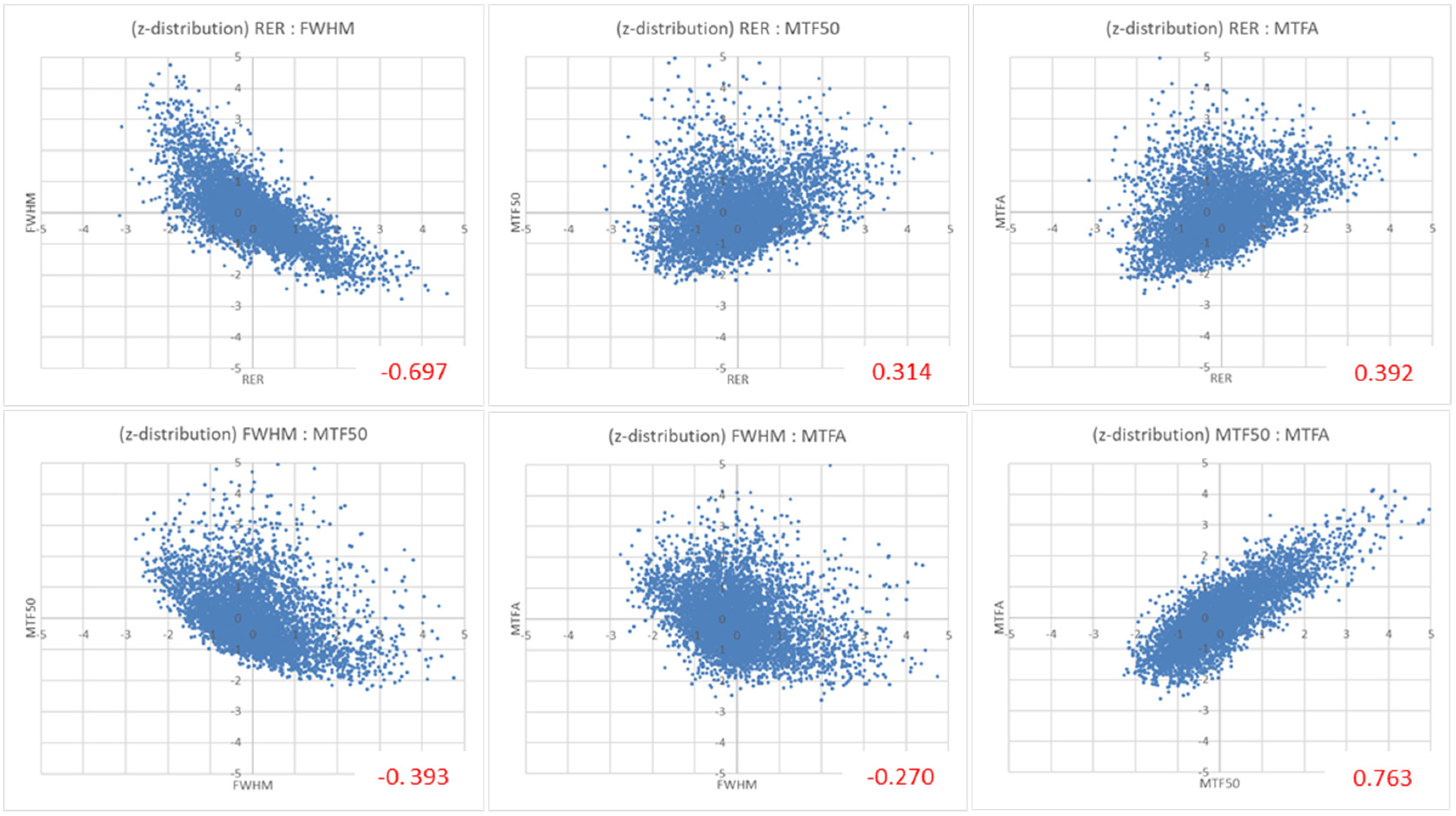
Figure 9 illustrates the correlation plots among RER, FWHM, MTF50, and MTFA, where the red numbers indicate the Pearson correlation coefficients. Table 6 summarizes the Pearson correlation coefficients between the spatial quality estimators derived from the Edge target and NT edge. The highest Pearson correlation coefficients are observed for RER versus FWHM in the spatial domain and for MTF50 versus MTFA in the frequency domain, indicating strong correlations within each respective domain. In contrast, the correlations between the spatial domain estimators (RER and FWHM) and the frequency domain estimators (MTF50 and MTFA) are relatively weak. This result implies that RER, FWHM, MTF50, and MTFA cannot individually represent the overall spatial quality of satellite imagery; rather, each estimator quantitatively characterizes only a specific aspect of spatial quality [1]. Except for the MTFA-related pairs (MTFA vs. RER, FWHM, and MTF50), the Pearson correlation coefficients derived from the Edge target with EdgeLine = 21 pixels and NT edge are generally similar. This observation is closely related to the MTFA measurement characteristics discussed in Table 5, and a more fundamental analysis of MTFA behavior is required in future work.

Figure 9. Scatter plots showing the relationships among RER, FWHM, MTF50, and MTFA. The bottom right values (in red) indicate Pearson’s correlation coefficients. The plot scales were converted to z-distributions.

Table 6. Pearson’s correlation coefficients between spatial quality estimators derived from the Edge target and NT edge.

Spatial Quality Estimator	Edge Target		NT Edge
	Full Edge	EdgeLine = 21	EdgeLine = 21
RER vs. FWHM	−0.718	−0.684	−0.697
RER vs. MTF50	0.419	0.244	0.314
RER vs. MTFA	0.248	0.082	0.392
FWHM vs. MTF50	−0.521	−0.375	−0.393
FWHM vs. MTFA	−0.244	−0.123	−0.270
MTF50 vs. MTFA	0.518	0.581	0.763

4.3. Summary

The mean spatial quality measurements derived from NT edges show RER and FWHM values comparable to those obtained from Edge targets with EdgeLine = 21 pixels, while MTF50 and MTFA tend to be higher for NT edges. The measurement precision, represented by the CV, is generally about two times worse for NT edges than for Edge targets with EdgeLine = 21 pixels. When excluding Phoenix (11 March 2021), which exhibits relatively high mean spatial quality values, the mean measurements become more similar across datasets, and the CV values are slightly reduced. The underlying reasons for the elevated spatial quality observed in Phoenix (11 March 2021) are not yet clear and require further investigation. Consistent with the results obtained from Edge targets with EdgeLine = 21 pixels, a comparison of CV values suggests that RER and FWHM tend to provide higher measurement precision than MTF50. In terms of relative precision, RER and FWHM appear to be more stable than MTF50. In cases where RER and FWHM cannot be reliably estimated, MTFA may serve as a complementary estimator, as it generally exhibits better precision than MTF50. However, the tendency of MTFA values derived from NT edges to be larger than those from Edge targets remains to be explained and warrants additional analysis. The main observations of this study can be summarized as follows:

• The NT edge-based spatial quality of KOMPSAT-3A remains stable over the analyzed time period, with no clear evidence of degradation attributable to sensor aging.
• No clear proportional relationship is observed between NT edge-based spatial quality and either roll tilt angle or edge angle.
• Weak correlations between spatial quality and ΔDN or SNR are suggested, although these trends are not strong.
• For Edge targets, a slight dependence on edge angle is observed, whereas no clear correlation with ΔDN or SNR is identified [1]. Compared with Edge targets, NT edges may be more influenced by higher-frequency noise components [41,42,43,44,45], but this effect has not been fully quantified.
• Relatively strong correlations are observed for RER versus FWHM and for MTF50 versus MTFA, while other relationships among spatial quality estimators appear weak or inconclusive.
• MTFA values derived from NT edges tend to be higher than those obtained from Edge targets with EdgeLine = 21 pixels, and MTFA-related Pearson correlation coefficients are also relatively high. A more detailed, physics-based analysis is required to better understand this behavior.

5. Conclusions

In this study, the spatial quality measurement results derived from 5531 NT edges extracted from multiple urban images acquired by KOMPSAT-3A were compared and analyzed. The results suggest that, when approximately 100 or more NT edges are available within a single urban image, the resulting mean spatial quality measurements can achieve a level of accuracy and precision that is potentially comparable to those obtained using Edge targets. As discussed in Section 4, the NT edge-based results do not always fully coincide with the spatial quality measurements derived from Edge targets with EdgeLine = 21 pixels [1], and some differences are observed that may be related to the influence of higher-frequency noise components. However, these noise-related effects do not appear to be the dominant factors governing the accuracy and precision of the mean spatial quality measurements obtained from NT edges. Although relatively high spatial quality values are observed for Phoenix (11 March 2021), the NT edge-based approach appears to be sufficiently reliable, from an availability perspective, to serve as an alternative to Edge targets for satellite image spatial quality assessment. One notable advantage of using NT edges is that spatial quality measurements can be performed within a single day, without the need for the construction, maintenance, and limited global availability of Edge targets, which currently number only a few worldwide. Consequently, NT edges provide a practical alternative for supplementing Edge target measurements or for situations in which Edge target imaging is not feasible.

Consistent with previous results obtained from Edge targets with EdgeLine = 21 pixels [1], the NT edge-based analysis indicates that RER and FWHM tend to provide higher measurement precision than MTF50. MTFA also shows relatively good precision when derived from NT edges; however, the tendency toward higher MTFA values requires further investigation to better understand the underlying causes.

Unlike the case of the Edge target [1], no clear correlation is observed between NT edge-based spatial quality and edge angle, while a weak correlation with SNR is suggested and warrants additional analysis. Since SNR inherently reflects the presence of higher-frequency noise components, this characteristic may partly explain the relatively higher MTF50 and MTFA values observed for NT edges.

Overall, this study indicates that NT edges can provide sufficient accuracy and precision for spatial quality measurement from an operational and availability standpoint. Based on the findings of this work, the following topics are identified for future investigation:

• Determination of the minimum number of NT edges required within a single urban image, based on an expanded dataset of KOMPSAT-3A urban acquisitions;
• Further analysis of the relationship between spatial quality measurements and higher-frequency noise components, particularly for frequency domain estimators such as MTF50 and MTFA;
• Investigation into the factors contributing to the relatively high spatial quality measurements observed for Phoenix (11 March 2021);
• Comparison of the proposed NT-edge-based results with spatial quality measurements obtained from other KARI satellite missions, including those of KOMPSAT-3 (GSD, 0.7 m; MTF50 > 8%), CAS500-1 (GSD, 0.5 m; MTF50 > 8%), and KOMPSAT-7 (GSD, 0.3 m; MTF50 > 6%).

References

- Lee, D.; Park, D.; Yoo, D. Precision and Characteristics of Satellite Spatial Quality Estimators’ Measurement Using an Edge Target Imaged with KOMPSAT-3A. Remote Sens. 2024, 16, 4660. [Google Scholar] [CrossRef] [Scilit]
- Lee, D.; Yoo, D. Introduction of Improvement of KARI’s MTF measuring Python algorithm. In Proceedings of the Korean Society of Remote Sensing—Fall Conference; The Korean Society of Remote Sensing: Busan, Republic of Korea, 2022; Available online: https://ksrs.or.kr/content/conferences/pre_reg_guide.php?id=86#n (accessed on 6 March 2026).
- Lee, D.; Park, D.; Helder, D.; Jeong, J.; Seo, D. Spatial Quality from Edge Target Imaged by KOMPSAT-3 (& KARI Methodology of MTF Estimation, ver. 2019) (Jan. 2014~July. 2019). JACIE 2019. USGS, USA. 2019. Available online: https://usgs.gov/calval/jacie-2019-presentations (accessed on 2 February 2026).
- Park, D.; Kim, H.; Seo, Y.; Jeong, J.; Seo, D.; Lee, D. Analysis on Refinement of On-orbit MTF Measurement using Edge Target. In VH-RODA 2019; ESA ESRIN: Frascati, Italy, 2019; Available online: https://earth.esa.int/eogateway/events/vh-roda-very-high-resloution-radar-optical-data-assessment-workshop-and-ceos (accessed on 2 February 2026).
- Lee, D.; Helder, D.; Christopherson, J.; Storey, J.; Seo, D.; Stensaas, G. RER, FWHM, MTF Processing Step for Edge Target (Draft) & Standard Edge Targets by KOMPSAT-3. CEOS WGCV IVOS-26. 2014. Available online: https://calvalportal.ceos.org/web/guest/ceos-wgcv/ivos/ivos-26 (accessed on 2 February 2026).
- Park, D.; Lee, D.; Jeong, J.; Seo, D.; Seo, Y. Validation of MTF Measurement Method by Edge Target. CEOS WGCV IVOS-30. 2018. Available online: https://calvalportal.ceos.org/web/guest/ivos-30 (accessed on 2 February 2026).
- Choi, T. IKONOS Satellite on Orbit Modulation Transfer Function (MTF) Measurement Using Edge and Pulse Method. Master’s Thesis, South Dakota State University, Brookings, SD, USA, 2002. [Google Scholar]
- Choi, T.; Helder, D. Generic Sensor Modeling for Modulation Transfer Function (MTF) Estimation. In Proceedings of the Pecora 16 “Global Priorities in Land Remote Sensing”, Sioux Falls, SD, USA, 23–27 October 2005. [Google Scholar]
- Viallefont-Robinet, F.; Helder, D.; Fraisse, R.; Newbury, A.; van den Bergh, F.; Lee, D.; Saunier, S. Comparison of MTF measurements using edge method: Towards reference data set. Opt. Express 2018, 26, 33625–33648. [Google Scholar] [CrossRef] [Scilit] [PubMed]
- Masaoka, K. Edge-based modulation transfer function measurement method using a variable oversampling ratio. Opt. Express 2021, 29, 37628–37638. [Google Scholar] [CrossRef] [Scilit] [PubMed]
- Masaoka, K. Enhancing Accuracy and Precision in Omni-Angle Edge-Based Modulation Transfer Function Measurements. IEEE Access 2025, 13, 20799–20809. [Google Scholar] [CrossRef] [Scilit]
- Pagnutti, S.; Blonski, D.; Cramer, M.; Helder, D.; Holekamp, K.; Honkavaara, E.; Ryan, R. Targets, methods, and sites for assessing the in-flight spatial resolution of electro-optical. Can. J. Remote Sens. 2010, 36, 583–601. [Google Scholar] [CrossRef] [Scilit]
- Blanc, P.; Wald, L. A review of earth-viewing methods for in-flight assessment of modulation transfer function and noise of optical spaceborne sensors. In HAL Open Science; hal-00745076; ESA ESRIN: Frascati, Italy, 2009. [Google Scholar]
- Blanc, P.; Wald, L. Image Quality—WP224 (ARMINES); TN-WP224-001-ARMINES; Issue 1.0; ESA ESRIN: Frascati, Italy, 2008. [Google Scholar]
- Viallefont-Robinet, F.; Helder, D.; Lee, D. Presentations in Geo/Spatial Quality Sub-Committee. CEOS WGCV IVOS-29. 2017. Available online: https://calvalportal.ceos.org/web/guest/ivos-29 (accessed on 2 February 2026).
- Viallefont-Robinet, F.; Legar, D. Improvement of the edge method for on-orbit MTF measurement. Opt. Express 2010, 18, 3531–3545. [Google Scholar] [CrossRef] [Scilit] [PubMed]
- Bowen, H.; Dial, G. IKONOS calculation of MTF using stellar images. In Proceedings of the 2002 High Spatial Resolution Commercial Imagery Workshop, Reston, VA, USA, 25–27 March 2002. [Google Scholar]
- Meygret, A.; Blanchet, G.; Mounier, F.; Buil, C. The Stars: An Absolute Reference for On-Orbit Calibration Application to PLEIADES 1A. CEOS WGCV IVOS-28. 2016. Available online: https://calvalportal.ceos.org/web/guest/ivos-28 (accessed on 6 March 2026).
- Meygret, A.; Latry, C.; Kelbert, A.; Blanchet, G. On-Orbit Star-Based Radiometric and Spatial Calibration of PLEIADES HR Optical Sensors. CEOS WGCV IVOS-31. 2019. Available online: https://calvalportal.ceos.org/web/guest/ivos-31 (accessed on 6 March 2026).
- Lee, D.; Storey, J.; Morfitt, R.; Choate, M.; Hayes, R.; Helder, D.; Stone, T.; Christopherson, J.; Stensaas, G. RER, FWHM, MTF from Landsat-8 OLI Lunar Data (Level 1R) (Draft). CEOS WGCV IVOS-26. 2014. Available online: https://calvalportal.ceos.org/web/guest/ceos-wgcv/ivos/ivos-26 (accessed on 2 February 2026).
- Choi, T.; Cao, C. NOAA-20 VIIRS On-Orbit Geometric Data Quality Estimation Using the Scheduled Lunar Collections. IEEE Trans. Geosci. Remote Sens. 2022, 60, 1003110. [Google Scholar] [CrossRef] [Scilit]
- Samadzadegan, F.; Aghvami, M.; Toosi, A.; Hasani, H.; Amini, O.; Ahadzadeh, S. On-orbit spatial resolution assessment of Khayyam satellite imagery using natural edge targets. Adv. Space Res. 2025, 76, 5014–5041. [Google Scholar] [CrossRef] [Scilit]
- Cenci, L.; Pampanoni, V.; Laneve, G.; Santella, C.; Boccia, V. Presenting a Semi-Automatic, Statistically-Based Approach to Assess the Sharpness Level of Optical Images from Natural Targets via the Edge Method. Case Study: The Landsat 8 OLI–L1T Data. Remote Sens. 2021, 13, 1593. [Google Scholar] [CrossRef] [Scilit]
- Park, M.; Kim, T. Applicability of ResNet-18 Based Transfer Learning for Quality Assessment of High-Resolution Satellite Images. Korean J. Remote Sens. 2025, 41, 301. [Google Scholar] [CrossRef] [Scilit]
- Javan, F.; Samadzadegan, F.; Toosi, A.; Schneider, M.; Persello, C. Ground Resolved Distance Estimation of Sentinel-2 Imagery Using Edge-based Scene-Driven Approach. PFG–J. Photogramm. Remote Sens. Geoinf. Sci. 2025, 93, 131–152. [Google Scholar]
- Kim, J.; Kim, T. Development of a natural target-based edge analysis method for NIIRS estimation. Korean J. Remote Sens. 2011, 27, 587. [Google Scholar] [CrossRef] [Scilit]
- Javan, F.; Samadzadegan, F.; Reinartz, P. Spatial Quality Assessment of Pan-Sharpened High Resolution Satellite Imagery Based on an Automatically Estimated Edge Based Metric. Remote Sens. 2013, 5, 6539–6559. [Google Scholar] [CrossRef] [Scilit]
- Pampanoni, V.; Cenci, L.; Laneve, G.; Santella, C.; Boccia, V. On-orbit image sharpness assessment using the edge method: Methodological improvements for automatic edge identification and selection from natural targets. In Proceedings of the IGARSS 2020-2020 IEEE International Geoscience and Remote Sensing Symposium; IEEE: New York City, NY, USA, 2020; pp. 6010–6013. [Google Scholar]
- CEOS WGCV IVOS. CEOS Cal/Val Portal—Cal/Val Sites. 2024. Available online: https://calvalportal.ceos.org/calvalsites (accessed on 2 February 2026).
- USGS EROS Cal/Val Center of Excellence (ECCOE). Test Sites Catalog—Spatial Sites Catalog. 2024. Available online: https://calval.cr.usgs.gov/apps/spatialsites_catalog (accessed on 2 February 2026).
- Niro, F.; Colombo, R.; Cogliati, S.; Genesio, L.; Miglietta, F.; Petitti, A.; Berthelot, B.; Saunier, S.; Morris, H.; Kuusk, J.; et al. Cal/Val Park: Project Status and Recent Updates; VH-RODA 2025; ESA ESRIN: Frascati, Italy, 2025. [Google Scholar]
- Coefficient of Variation (CV). WIKIPEDIA. Available online: https://en.wikipedia.org/wiki/Coefficient_of_variation (accessed on 2 February 2026).
- Lee, D.; Yoo, D. Python algorithm for measuring the Spatial quality (RER, FWHM, MTF) on the Edge of Terrain feature. In Proceedings of the 28th ISRS (International Symposium on Remote Sensing), Jeju, Republic of Korea, 19–21 April 2023. [Google Scholar]
- Lee, D. Comparison of results of applying Savitzky-Golay filter to improve the result value and precision of Edge Spatial quality Measurement Python code (ESMP, ver. 2025.04.24). In Proceedings of the Korean Society for Aeronautical and Space Sciences (KSAS) Space Science Conference 2025, Yeosu, Republic of Korea, 25–27 June 2025; Available online: https://ksas.or.kr/Conference/ConferenceView.asp?AC=0&CODE=CC20250301 (accessed on 2 February 2026).
- Lee, D. Analysis of Differences in Spatial Quality Measurement Results According to the Order of Application of the SGolay Filter and CSAPS in ESF Fitting; KARI Research Note; KARI-CVIQRT-ELN-2025-008; KARI: Daejeon, Republic of Korea, 2025.
- Lee, D. Reliability Items related within Edge target’s Spatial quality measurement Python code, and Issues of Input number of EdgeWidth (Pixel line) and CSAPS fitting. In Proceedings of the Korean Society of Remote Sensing—Fall Conference, Gyeongju, Republic of Korea, 15–17 November 2023; Available online: https://ksrs.or.kr/content/conferences/pre_reg_guide.php?id=87 (accessed on 6 March 2026).
- Lee, D.; Yang, J.; Seo, D.; Song, J.; Chung, J.; Lim, H. Image Restoration from Asymmetric Point Spread Function of High Resolution Remote Sensing Satellite with Time Delayed Integration. Adv. Space Res. 2011, 47, 690–701. [Google Scholar] [CrossRef] [Scilit]
- Wu, K.; Yang, M. Mean shift-based clustering. Pattern Recognit. 2007, 40, 3035–3052. [Google Scholar] [CrossRef] [Scilit]
- Yoo, D.; Lee, D.; Choi, S.; Jin, K. Region of Interest Detection Algorithm for Satellite Image Landmark-based MTF Measurement. In Proceedings of the Korean Society for Aeronautical and Space Sciences (KSAS) 2021 Fall Conference, Jeju, Republic of Korea, 17–19 November 2021; Available online: https://ksas.or.kr/Publications/sub_05_12.asp (accessed on 2 February 2026).
- CharGPT. ‘Question: What Is the Minimum Sample Size Statistically?’. ChatGPT. 2025. Available online: https://chatgpt.com (accessed on 30 December 2025).
- Lee, D. Analysis of the Influence of Noise Amount on ESF and ESF Fitting; KARI Research Note; KARI-CVIQRT-ELN-2025-009; KARI: Daejeon, Republic of Korea, 2025.
- Kuhls-Gilcrist, A.; Jain, A.; Bednarek, D.; Hoffmann, K.; Rudin, S. Accurate MTF measurement in digital radiography using noise response. Med. Phys. 2010, 37, 724–735. [Google Scholar] [CrossRef] [Scilit] [PubMed]
- Haefner, D.; Burks, S. Noise estimation of an MTF measurement. In Proceeding of SPIE Vol. 8355 Infrared Imaging Systems: Design, Analysis, Modeling, and Testing XXIII; SPIE/International Society for Optical Engineering: Bellingham, WA, USA, 2012; Available online: http://proceedings.spiedigitallibrary.org (accessed on 2 February 2026).
- Zwanenberg, O.; Triantaphillidou, S.; Jenkin, R.; Psarrou, A. Estimation of ISO12233 Edge Spatial Frequency Response from Natural Scene Derived Step-Edge Data. J. Imaging Sci. Technol. 2021, 65, 060402–1–060402-16. [Google Scholar] [CrossRef] [Scilit]
- Pampanoni, V.; Fascetti, F.; Cenci, L.; Laneve, G.; Santella, C.; Boccia, V. Analysing the Relationship between Spatial Resolution, Sharpness and Signal-to-Noise Ratio of Very High Resolution Satellite Imagery Using an Automatic Edge Method. Remote Sens. 2024, 16, 1041. [Google Scholar] [CrossRef] [Scilit]
Disclaimer/Publisher’s Note: The statements, opinions and data contained in all publications are solely those of the individual author(s) and contributor(s) and not of MDPI and/or the editor(s). MDPI and/or the editor(s) disclaim responsibility for any injury to people or property resulting from any ideas, methods, instructions or products referred to in the content. |
© 2026 by the authors. Licensee MDPI, Basel, Switzerland. This article is an open access article distributed under the terms and conditions of the Creative Commons Attribution (CC BY) license.