Characterization of Local and Long-Distance Ice Floe Motion in the Yellow River Using UAV–GPS Joint Observations

Highlights

What are the main findings?

• The use of unmanned aerial vehicle (UVA) and global positioning system (GPS) joint observation has obtained various motion parameters of ice floes, including motion velocity vector field, lateral velocity gradient, rotational angular velocity, rotational direction, long-term motion distance, time, and average velocity of ice floes.
• The rotation of ice floe is positively correlated with the velocity gradient, and the direction of rotation is related to the positive or negative value of the velocity gradient.

What are the implications of the main findings?

• This study applies a UAV–GPS joint observation approach to river ice motion monitoring, enabling the characterization of ice movement from local zones (100 m–300 m) to long-distance (over 10 km) transport.
• This study demonstrates the potential of integrated UAV and in situ remote sensing for refined river ice monitoring, providing transferable remote sensing parameters for ice hazard assessment and modeling in cold-region rivers.

Abstract

Understanding the motion parameters of floating ice is very important for characterizing the ice water dynamics of rivers during freezing periods. Due to the low spatiotemporal resolution of satellite images, limited observation range of unmanned aerial vehicles, and deformation of shore-based camera images, it is difficult to simultaneously quantify the translational and rotational motion characteristics of floating ice and long-distance transportation. This study used the unmanned aerial vehicle GPS joint observation method to observe and obtain various motion parameters such as local translation, rotation, and long-distance transportation in the curved section of the upper reaches of the Yellow River and the straight section of the middle reaches of the Yellow River during the winter of 2024–2025 under conditions of ice density of 50–90%. The velocity field obtained by the drone shows an average ice velocity of 1.27 m/s at the bend and 1.18 m/s in the straight section, with lateral velocity gradients of −0.245 to 0.050 s⁻¹ and −0.141 to 0.222 s⁻¹, respectively. The angular velocity of a single floating ice block is 0.008–0.016 rad/s at bends and 0.010–0.036 rad/s in straight sections. The angular velocity is positively correlated with the local shear strength, and the rotation direction is consistent with the sign of the velocity gradient. GPS tracking provides long-distance transportation trajectories, and the average difference between the speeds obtained by GPS and drones is 0.10 m/s, confirming the reliability of speed estimation based on drones. These results indicate that integrated unmanned aerial vehicle GPS observation can quantitatively characterize local floating ice movement and long-distance floating ice transport behavior, providing on-site parameters for river ice water dynamics research and hazard assessment, and has the potential to be applied to rivers in other cold regions.

1. Introduction

River ice motion parameters are critical indicators for monitoring river ice processes during the freeze-up period and play an important role in understanding ice jam and ice dam formation mechanisms, validating river ice numerical models [1], and supporting hazard forecasting and mitigation. As a typical river in northern China with frequent ice-related hazards [2], the Yellow River experiences complex ice processes during the freeze-up season. Accurate observation of ice floe motion characteristics during this period is essential for advancing ice–water dynamics research and improving river ice hazard prevention and control.

Satellite remote sensing has been widely applied to large-scale observations of river ice types, spatial distribution, ice coverage, and ice break-up [3]. However, due to limitations in spatial and temporal resolution, satellite imagery has rarely been used for ice velocity observation. Optical satellite data commonly used for river ice monitoring include AVHRR [4], Landsat [5], MODIS [6], Sentinel-2 [7], and Gaofen [8], while microwave satellite data include Sentinel-1 [9], RADARSAT-1 [10], and RADARSAT-2 [11]. Methods for extracting river ice parameters from satellite data mainly include manual visual interpretation [12], threshold-based classification [13], K-means clustering [14], and random forest classification [15]. Yang et al. [16] used Landsat imagery from 1984 to 2018 to reveal the global distribution of river ice, analyze historical changes, and predict future trends. Li et al. [17] applied Landsat imagery and the NDSI algorithm to characterize the spatiotemporal distribution of river ice on the Tibetan Plateau at the basin scale, showing a decreasing trend in ice-covered area from 1999 to 2018. Altena [18] estimated ice velocities along more than 700 km of the Lena River in Russia using Sentinel-2 and PROBA-V data and discussed an upper temporal separation limit of 30 s for ice velocity estimation based on satellite imagery.

Existing satellite remote sensing technology faces major technical limitations in river ice observation, especially in balancing spatial and temporal resolutions. For ice floes with typical scales less than 2 m during the ice flood season of the Yellow River, although their translational characteristics can be obtained through various means, it remains significantly challenging to simultaneously capture the rotational behavior of the ice floes and effectively link local fine movements with long-distance transport processes. To address this challenge, scholars have developed various shore-based observation methods. For example, Bourgault [19] designed a tilt image correction method based on ground control points (latitude, longitude, and altitude) to calculate the concentration of ice floes in the river channel; Pei [20] utilized deep learning algorithms to segment ice–water images and subsequently obtain the concentration of ice floes; Deng et al. [21] designed a remote automatic monitoring system for river ice, which enables continuous monitoring of multiple parameters of floating ice in curved areas through shore-based cameras; Daigle et al. [22] applied the Particle Image Velocimetry (PIV) particle tracking method to track the movement of ice floes in the St. Lawrence River, obtaining ice flow velocity information.

In recent years, UVA remote sensing has developed rapidly in river ice monitoring. Due to its maneuverability, centimeter-level spatial resolution, and high temporal sampling frequency, drone-based observations have become an effective tool for capturing fine-scale river ice processes that are difficult to solve with satellite images. Research on river ice based on drones can be classified into the following categories:

• The identification and evaluation of ice jams and ice dams have been extensively explored. Wang et al. [23] and Alfredsen et al. [24] demonstrated that aerial measurements based on drones provide effective support for monitoring ice-related flood disasters. Alfredsen and Juarez [25] further applied motion structure (SfM) photogrammetry to generate a digital elevation model (DEM) of the ice surface, enabling non-contact detection of ice jam geometry and spatial distribution. Subsequent work will combine the ice geometry obtained by drones with airborne LiDAR data to construct a detailed riverbed ice terrain model for simulating the hydraulic effects of ice jams.
• Ice thickness monitoring using UAV-borne ground-penetrating radar (GPR) has been developed. Li et al. [26] investigated the spatiotemporal evolution of ice thickness in a Yellow River bend and corrected radar wave velocity using air temperature and measured ice thickness. Meng et al. [27] designed a UAV-mounted GPR system for river and lake ice detection and proposed an automatic time-picking algorithm based on energy ratios and cross-correlation analysis. Bai et al. [28] developed a layer tracking method for UAV-mounted GPR data to improve ice thickness inversion accuracy under layered ice conditions.
• Ice–water image recognition and segmentation techniques have evolved from traditional image processing to machine learning and deep learning approaches. Kalke and Loewen [29] applied support vector machines (SVMs) for ice classification in the North Saskatchewan River. Singh et al. [30] introduced deep learning models for river ice segmentation. Ansari et al. [31] developed IceMaskNet based on an improved Mask R-CNN framework for detecting multiple ice types, including frazil ice, broken ice, and border ice. Zhang et al. [32,33] proposed ICENET and ICENETv2 networks incorporating attention mechanisms to improve fine-grained segmentation of thin ice and fragmented ice under complex Yellow River backgrounds.
• Ice floe geometric parameter extraction and velocity estimation have received increasing attention. Blotnicki et al. [34] quantified ice floe morphological characteristics such as area, perimeter, mean size, and circularity from UAV imagery to assess blockage risk. Möldner [35] applied particle image velocimetry (PIV) to oblique UAV video to estimate cross-sectional ice velocities. Wang et al. [36] employed a UAV-SIFT feature tracking algorithm to estimate local ice velocity and flow direction, focusing primarily on translational motion within limited spatial domains.

However, the methods still have certain limitations. Under complex field conditions, shore-based camera technology is susceptible to image tilt and deformation caused by ice floes, as well as constraints on the observation field of view, making it difficult to accurately capture the rotational details of ice blocks. Furthermore, as shown in

Table 1. A comparison of remote sensing observation scales and ice floe characteristic scales in the Yellow River.

Object	Spatial Scale	Temporal Scale	Suitability for Ice Floe Motion Identification
Yellow River channel width	150–300 m	—	Background scale
Single ice floe	<2 m	Seconds	Study object
MODIS	250–500 m	1–2 passes/day	Cannot resolve individual floes
Landsat 8/9	15–30 m	16 days	Insufficient spatial and temporal resolution
Sentinel-2A/2B	10 m	5 days (N 39°–N 41°)	Difficult to capture translation and rotation
UAV vertical video	0.05 m *	1 s	Capable of resolving translation and rotation

* The drone is flying at an altitude of 100 m.

, there is a significant spatial scale difference between the characteristic scale of ice floes and the width of river channels (typically 150–300 m). Existing free satellite remote sensing data cannot simultaneously meet the requirements of identifying individual ice blocks and monitoring movement processes at high frequencies in terms of spatiotemporal resolution. In contrast, unmanned aerial vehicle (UAV) vertical video imagery highly matches the scale of ice floes in terms of spatial resolution and temporal sampling frequency, making it a feasible observation method for analyzing the translational and rotational motion characteristics of ice floes.

To address these challenges, this study conducted field experiments during the 2024–2025 freeze-up season of the Yellow River, integrating high-resolution UAV imagery with throw-and-drop GPS tracking to investigate drifting ice floe motion in both meandering and straight channel reaches. Compared with previous UAV-based river ice motion studies, the present work advances the field in three key aspects:

• A UAV-GPS joint remote sensing observation framework has been established, connecting the local short-distance movement characteristics of ice blocks with the kilometer-scale long-distance transport process;
• Based on high-resolution on-site imagery, rotational motion parameters of individual ice blocks were extracted and quantified, providing empirical evidence for the dynamics of river ice rotation;
• The velocity field inverted by the drone was verified on site using the ice flow velocity independently obtained by GPS.

2. Study Area, Joint Observation Technology, and Data Processing

2.1. Study Area

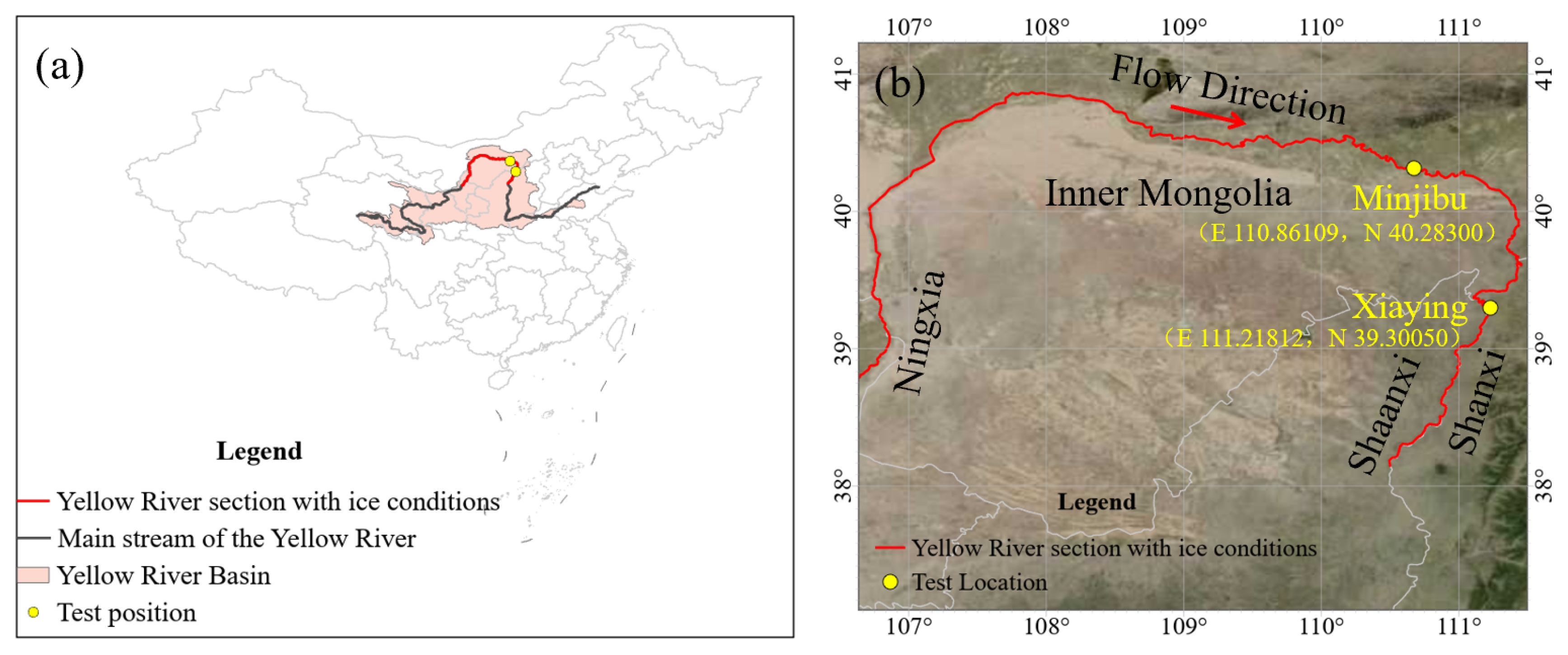
The Yellow River is the second longest river in China, with a total length of approximately 5464 km and a drainage area of about 795,000 km² (Figure 1a). During winter, ice processes occur in the upper Ningxia–Inner Mongolia reaches and the middle Shanxi–Shaanxi reaches due to the river’s unique geographical location, climatic conditions, and its characteristic “Ω-shaped” course spanning low to high latitudes. These ice processes can damage river engineering structures and bridges, and in severe cases lead to levee breaches and ice-related flood hazards [37]. The Inner Mongolia reach in the upper Yellow River is located at the northernmost part of the basin, extending approximately 840 km. This reach is characterized by gentle longitudinal slopes and numerous bends and is one of the most typical and ice hazard-prone sections of the Yellow River. The freeze-up period generally begins in mid-to-late November, followed by complete freeze-up in early to mid-December, and break-up in mid-to-late March of the following year, lasting approximately 4–5 months. Owing to the south-to-north flow direction of the river, downstream sections freeze earlier than upstream sections, while thawing occurs first upstream and later downstream. The middle reaches of the Yellow River in Shanxi and Shaanxi provinces extend for approximately 725 km and are characterized by canyon-type channels with relatively steep slopes and high flow velocities. During winter, river ice in this reach mainly exists in the form of drifting ice floes. Field experiments for observing ice floe motion were conducted on 8 December 2024 at the Minjibu bend in Inner Mongolia and on 7 January 2025 at the Xiaying straight channel in Shanxi Province (Figure 1b).

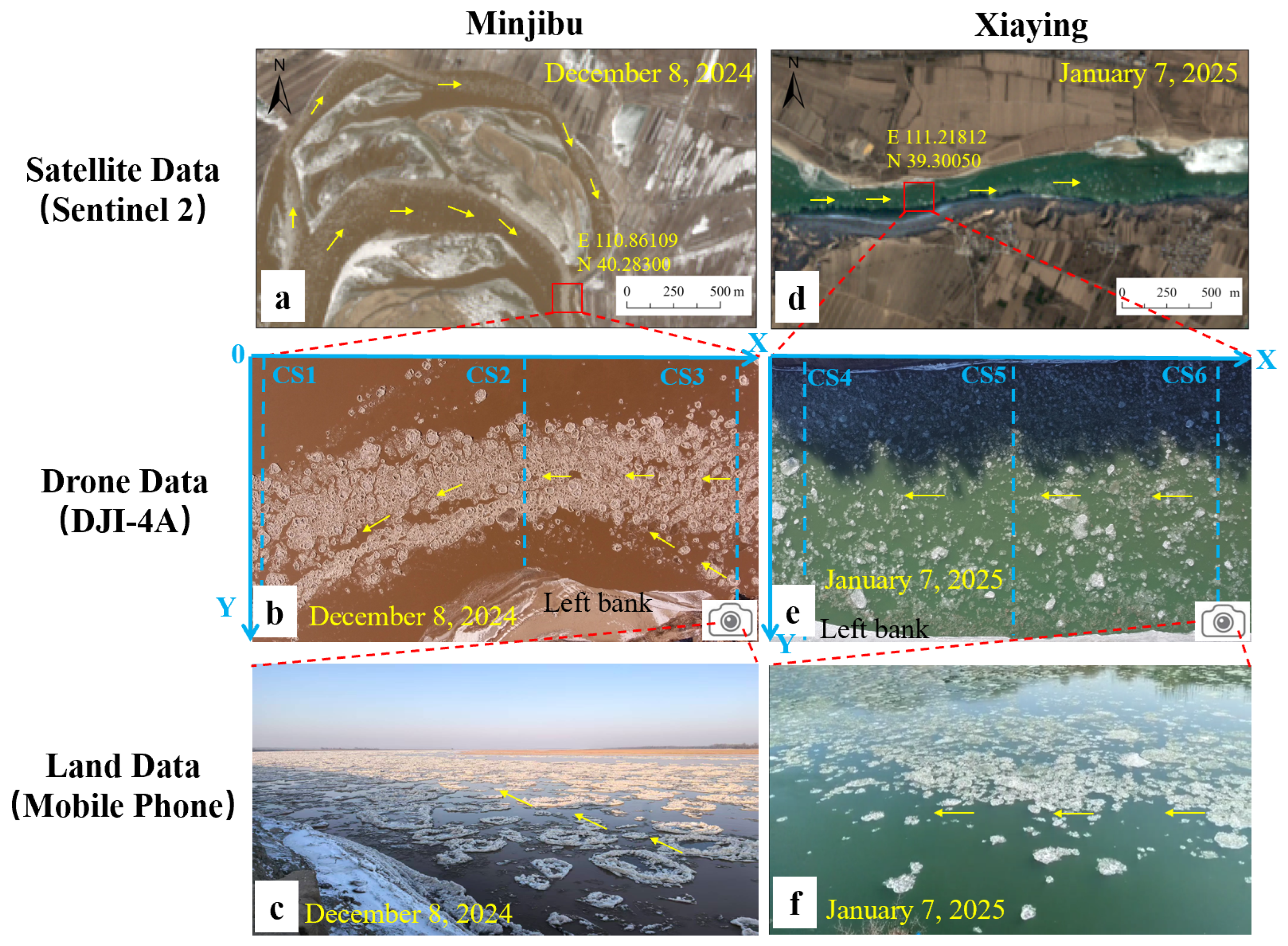
The Minjibu bend (E 110.86109, N 40.28300) is in Togtoh County, Inner Mongolia, and represents a typical Ω-shaped bend of the Yellow River. The channel width ranges from approximately 110 to 390 m. A large shallow shoal is present in the middle of the bend, dividing the flow into two branches and forming a double-bend channel configuration (Figure 2a). The field experiment was conducted in the downstream confluence zone of the bend, where two drifting ice streams merge and flow downstream. The UAV observation area has a channel width of approximately 90 m, with an ice floe concentration of about 50–80%. Three ice velocity observation cross-sections were established within the study area (Figure 2b). Field observations indicate that the drifting ice floes are irregular, round-shaped plates with white curled edges, and the river water appears brownish-yellow in color (Figure 2c).

The Xiaying straight channel (E 111.21812, N 39.30050) is in Hequ County, Shanxi Province, with a channel length of approximately 2.1 km and a channel width ranging from about 80 to 170 m (Figure 2d). The experiment was conducted in the middle section of the straight channel, where shore ice is present along the left bank and the right bank consists of exposed land. The UAV observation area has a channel width of approximately 90 m, with an ice floe concentration of about 50–90%. Ice floe concentration is higher near the right bank and lower near the left bank. Three ice velocity observation cross-sections were established within the study area (Figure 2e). Field observations show that the drifting ice floes are pure white irregular plates, and the river water appears green in color (Figure 2f).

2.2. UAV Video and GPS Joint Technology

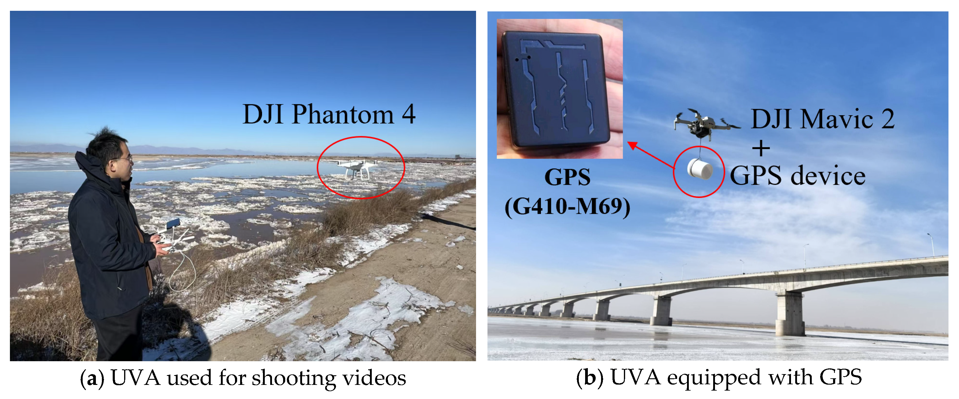
Figure 3a illustrates the joint observation scheme for drifting ice floe motion using UAV video imagery and GPS tracking. Two UAVs were deployed during the field experiments: one UAV was positioned upstream to deploy GPS devices onto selected drifting ice floes, while the other UAV hovered downstream to acquire vertical video imagery of ice floes passing through the observation area. This configuration ensured that ice floes equipped with GPS devices could be captured within the UAV video observation domain.

Table 2. Technical specifications.

UAV Video		GPS
type	DJI-4	type	DJI-Mavic 2
flying height	100 m	flying height	5 m
shooting method	Fixed-point vertical shooting	projector	line thrower
shooting time	4 min 25 s	GPS type	G410-M69
FOV	84°	GPS size	33 × 30 × 15 mm
image pixel	20 million	GPS battery	900 mAh
video resolution	3840 × 2160	GPS weight	21 g
video frame rate	30 frame/s	GPS positioning frequency	10 s
ground pixel size	5 cm	GPS positioning error	5 m

shows the technical parameters.

Phantom 4 UAV (DJI, Shenzheng, China) (Figure 3a) was used to acquire vertical video imagery of ice floes. The UAV hovered at an altitude of 100 m and recorded videos for approximately 5 min at fixed locations. The camera had a field of view (FOV) of 84°, with a video resolution of 3840 × 2160 pixels and a frame rate of 30 frames per second. The resulting ground sampling distance of the video imagery was approximately 5 cm. DJI Mavic 2 UAV was used to deploy GPS devices onto drifting ice floes (Figure 3b). The UAV flew at an altitude of approximately 5 m and was equipped with a remotely controlled line-type release mechanism. UVA flight occurred under clear weather conditions, with an air temperature of −5.28 °C, wind speeds of 2–6 m/s, and cloud cover of approximately 10–15%. Each battery has a flight time of about 20 min.

The Mavic 2 (DJI, Shenzheng, China) used for GPS deployment operated at an approximate flight height of 5 m above the river surface. A remotely controlled rotating hook was mounted beneath the UAV. Each GPS unit was enclosed in a small white plastic container to ensure waterproofing and visibility. The container was connected to the hook using a thin line. During deployment, the DJI Mavic 2 was positioned upstream of the observation area. Using the wireless remote control, the hook was rotated to detach the plastic container, allowing the GPS unit to drop onto the surface of drifting curled ice floes. At each study site, three GPS units were deployed, all successfully landing on ice floes and providing valid positioning data.

During experiments, DJI Phantom 4 UAV was first positioned above the target reach to capture vertical video of ice motion. The DJI Mavic 2 drone is equipped with GPS and then takes off to the upstream of the video drone. By using a remote hook device, the white plastic equipped with GPS falls onto the surface of the floating ice. To ensure the synchronization of drone video time and GPS sampling time, when observing the movement of floating ice with plastic buckets entering the drone shooting range, we selected images with GPS time and drone video time that are the same and took the average velocity of drone floating ice within 10 s.

The GPS device model is G410-M69, with dimensions of 33 × 30 × 15 mm, a weight of 21 g, and a battery capacity of 900 mAh. The positioning interval was 10 s, and the positioning accuracy was approximately 5 m.

2.3. UAV Video Image Processing

At the Minjibu bend, 3 min and 23 s of vertical UAV video imagery were acquired, while at the Xiaying straight reach, 1 min and 2 s of vertical UAV video imagery were collected. The videos were segmented into image frames at a temporal interval of 1 s, resulting in 203 image frames for the Minjibu reach and 62 image frames for the Xiaying straight channel.

Particle image velocimetry (PIV) was applied to the UAV image sequences to estimate ice floe motion velocities, directions, and streamlines in different river sections. Specifically, the PIVlab toolbox [38,39] (Version 3.12.001) implemented in MATLAB (R2015a) was used to compute velocity vector fields from the image sequences, yielding instantaneous velocities, mean velocities, velocity directions, streamlines, and cross-sectional ice velocities.

The 64 × 64-pixel window selected for this study follows the standard recommendations of the PIVlab toolbox for high-resolution image sequences [38,39]. Taking into account the ground sampling distance (~0.05 m) and typical ice floe displacement (approximately 1.3 to 1.6 m per second), the selected window size strikes a balance between spatial resolution and vector stability.

According to previous PIV accuracy evaluations under comparable imaging conditions, velocity uncertainty is typically within 2–5%. Furthermore, the mean absolute difference between UAV-derived velocities and independent GPS measurements (0.10 m/s) suggests that the adopted PIV configuration yields reliable velocity estimates at the scale of interest.

To analyze the velocity differences across the cross-section interpreted by PIV, Formula (1) is introduced to calculate the velocity gradient across the cross-section, thereby characterizing the shear rate of the flow.

$$VG={\displaystyle \frac{\mathsf{\partial }u}{\mathsf{\partial }y}},$$

(1)

where $VG$ is the profile velocity gradient (s⁻¹); $\mathsf{\partial }u$ is the profile velocity (m/s); $\mathsf{\partial }y$ is the distance (m)

Under highly dynamic river ice conditions, accurate ground-truth datasets describing both translational and rotational motion of individual drifting ice floes are extremely scarce. During ice floe motion, ice floes frequently undergo rotation, collision, and partial occlusion, posing significant challenges for existing automated image-based tracking algorithms. Preliminary tests conducted in this study indicate that such automated methods often fail to reliably preserve rigid-body rotation and boundary integrity of individual ice floes, leading to substantial errors in both translational velocity and angular motion estimation. Therefore, a high-precision manual supervision approach was adopted to extract the outer contours and motion directions of individual ice floes at 5 s intervals. Manual contour extraction required approximately 10–20 s per ice floe, depending on image clarity and floe shape complexity. For each study site, the total processing time was approximately half an hour. Although time-consuming, this approach ensures the acquisition of fine-scale kinematic details under complex motion patterns and provides a reliable reference dataset for validating GPS-based trajectories and assessing the limitations of automated remote sensing algorithms.

Based on the extracted ice floe contours at different time steps, the centroid of each ice floe was determined, and the translational trajectory of an individual ice floe was obtained by connecting the centroids. The translational velocity of an individual ice floe was calculated using Equations (2) and (3), while the rotational angle was calculated using Equation (4).

$$D_{ice\_single}=\sqrt{{\left(X_{m+1}-X_m\right)}^2+{\left(Y_{m+1}-Y_m\right)}^2},$$

(2)

$$V_{ice\_single}={\displaystyle \frac{D_{ice\_single}}{t}},$$

(3)

where $D_{ice\_single}$ is the distance between time $m+1$ and $m$; $V_{ice\_single}$ is the velocity between time $m+1$ and $m$; $t$ is time between time $m+1$ and $m$; $(X_m,Y_m)$ is coordinates in time $m$; $(X_{m+1},Y_{m+1})$ is coordinates in time $m+1$.

Rotation angle was computed as follows:

$$R_{ice\_single}=A_{m+1}-A_m,$$

(4)

where $R_{ice\_single}$ is the rotation angle; $A_{m+1}$ is the angle between a feature line and the north axis at time $m+1$; $A_m$ is the angle between a feature line and the north axis at time $m$.

2.4. GPS Data Processing

GPS tracking was used to monitor the long-distance transport of drifting ice floes within the river channel, with a sampling interval of 10 s. The raw GPS data were recorded in the WGS-84 geographic coordinate system, including latitude and longitude information for each time step. For accurate calculation of motion distances and velocities, all GPS data were projected into the UTM coordinate system (Zone 49N) to obtain planar coordinates.

Due to the complex river environment, water surface reflections, and signal obstruction, the raw GPS trajectories exhibited temporal discontinuities and occasionally contained anomalous points located outside the river channel. Sentinel-2 high-resolution optical imagery was used to delineate the river channel boundaries and the physically reasonable activity range of drifting ice floes. GPS points falling outside the channel boundaries were identified and removed based on spatial consistency criteria.

Only valid GPS points located within the river channel were used for subsequent calculations. The displacement between adjacent valid GPS points was calculated using planar coordinate differences and combined with the corresponding time intervals to derive instantaneous velocities. The total travel distance, duration, and mean velocity of individual ice floes were then computed. This data processing procedure ensured that all motion parameters were derived directly from observed GPS data, thereby minimizing the influence of data filtering on the inversion of ice floe motion characteristics.

GPS velocity uncertainty was further evaluated and is discussed in Section 4.3.

2.5. Data Processing Flow and Parameter Acquisition Framework for Joint Observation Scheme

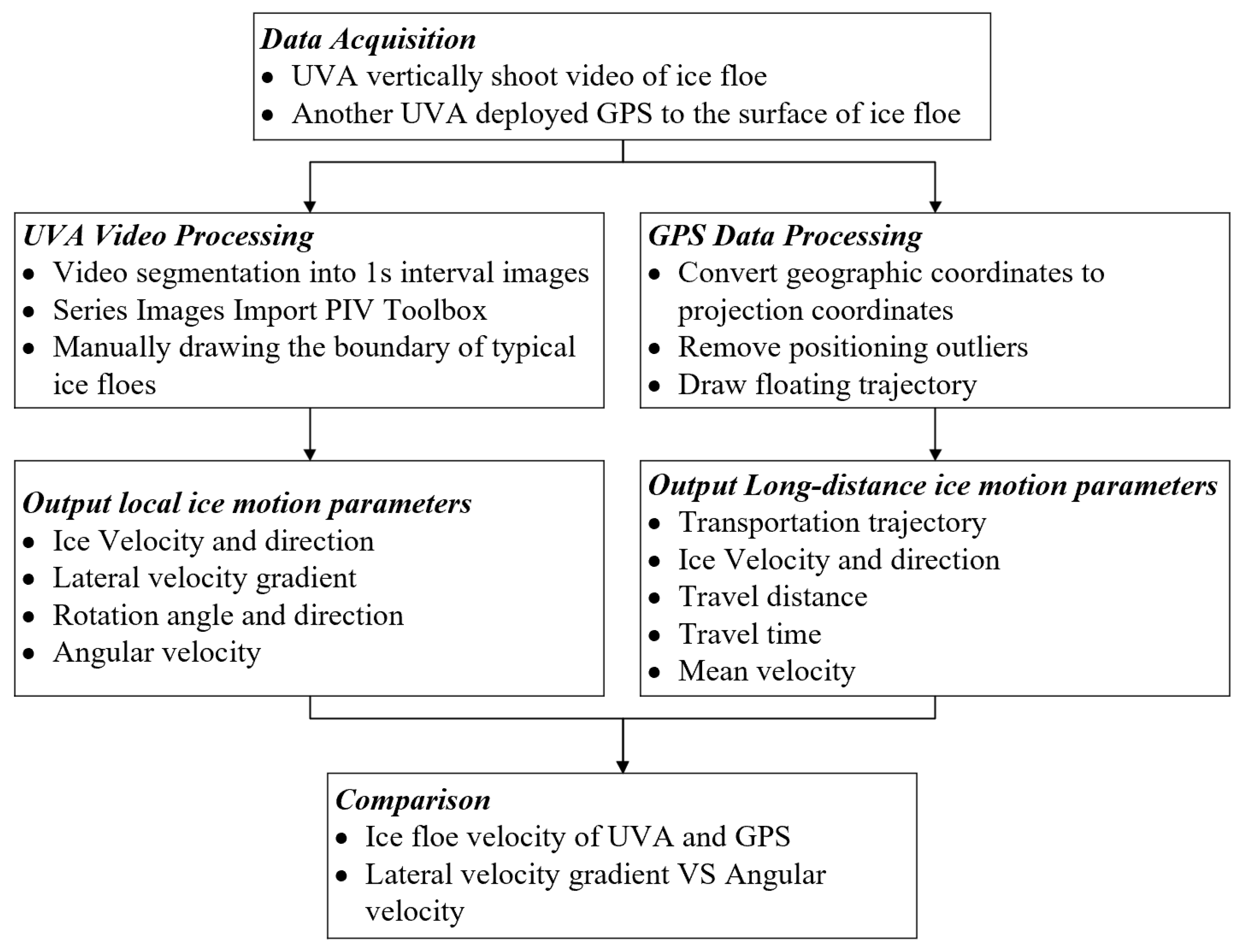
To achieve systematic characterization of ice floe motion at different spatial scales, this study constructs a joint observation data processing flow based on UAV vertical video imagery and throw-and-drop GPS devices, as shown in Figure 4.

As illustrated in Figure 4, UAV video data are primarily used to invert local ice floe velocity vector fields and streamlines and extract the translational trajectories and rotational characteristics of individual ice floes. GPS data, on the other hand, are used to obtain the ice floe motion trajectories, travel distances, durations, and mean velocities at the kilometer scale. Based on these, a comparison and consistency check of the velocities obtained from UAV and GPS results is performed to establish the scale linkage between local motion features and long-distance transport processes, ultimately generating a multi-scale ice floe motion parameter product that provides a unified data foundation for subsequent result analysis and applications.

3. Results

3.1. Short-Distance Ice Floe Velocity Field Characteristics

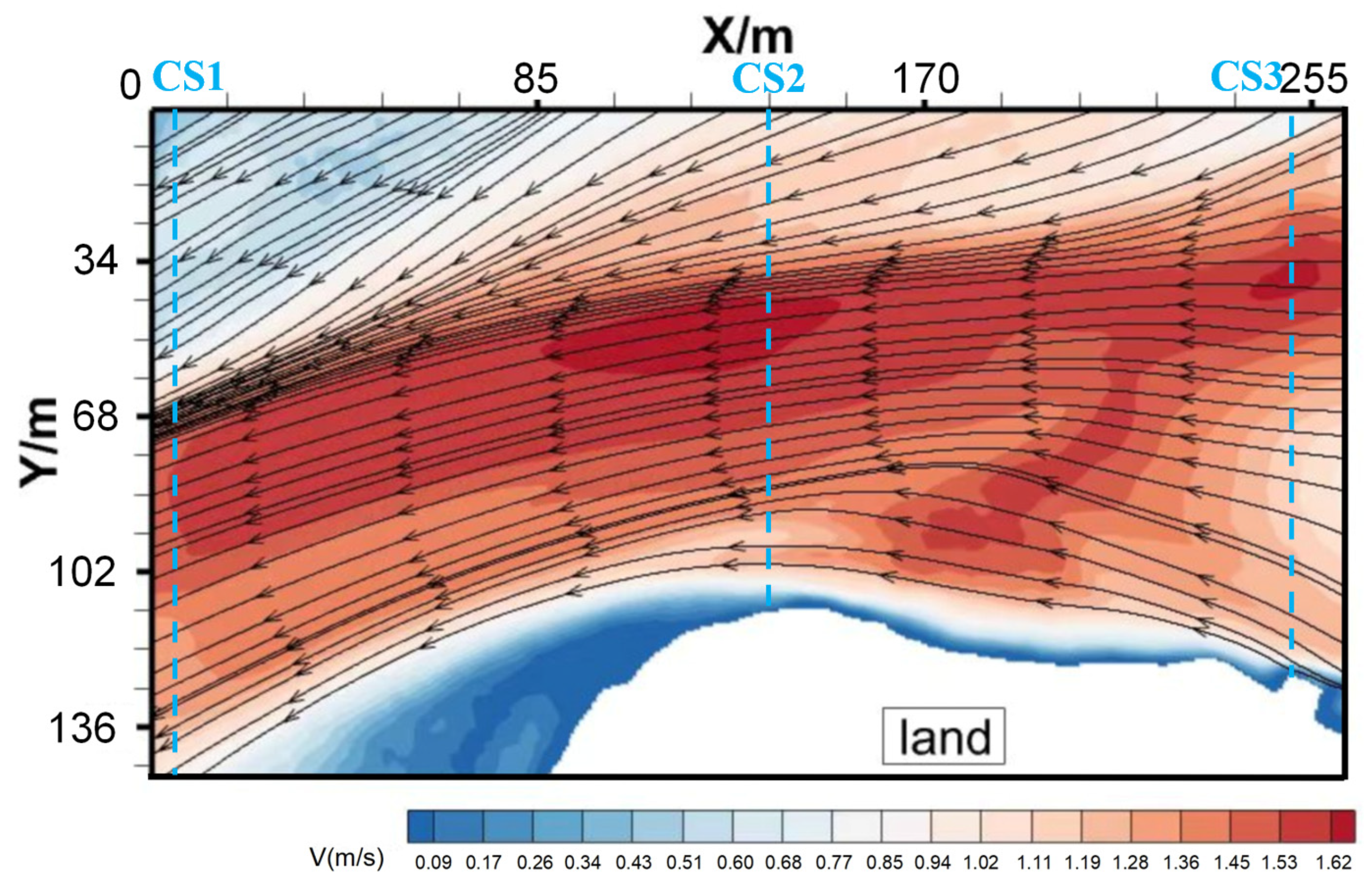
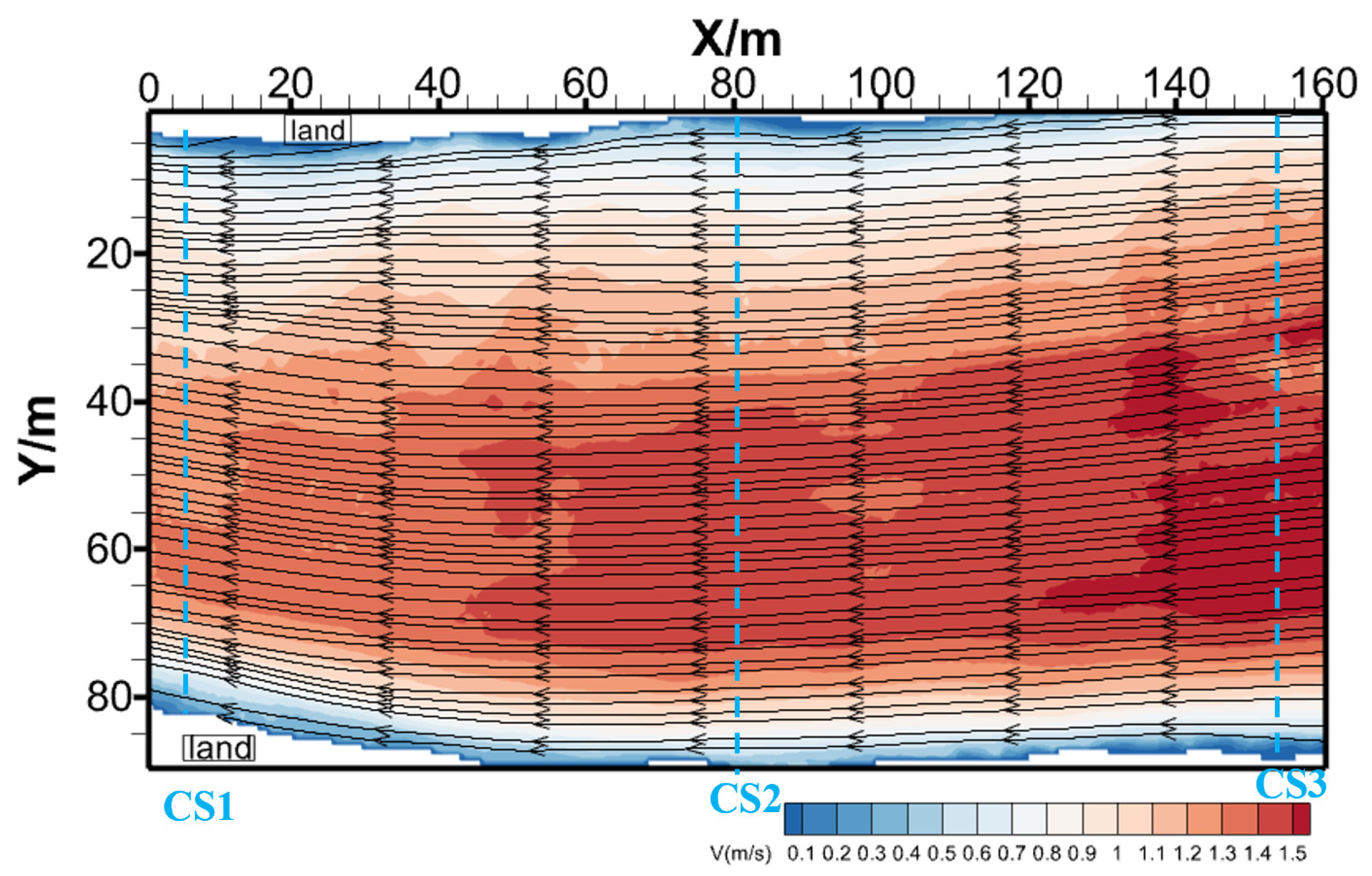
Based on UAV vertical video imagery and the PIV method, the spatial distribution patterns of ice floe velocities and the velocity field characteristics were inverted for both the Minjibu bend and the Xiaying straight channel (Figure 5 and Figure 6) as well as the typical cross-sectional characteristics (Figure 7 and Figure 8). The results show that, whether in the bend or straight river sections, the velocity profiles obtained through video interpretation generally comply with basic hydraulic laws of the river channel, presenting significant lateral variation.

In the Minjibu bend (Figure 5), the convergence effect of the streamlines is obvious, with the ice floes showing a tendency to gather toward the high-speed mainstream zone. This is because under the influence of centrifugal force on the curve, the surface water flow is pushed towards the outer bank, enhancing the velocity in the middle of the river channel. In the Xiaying straight channel (Figure 6), the streamlines are nearly parallel to the riverbank, and the velocity distribution follows the boundary layer theory of the river channel.

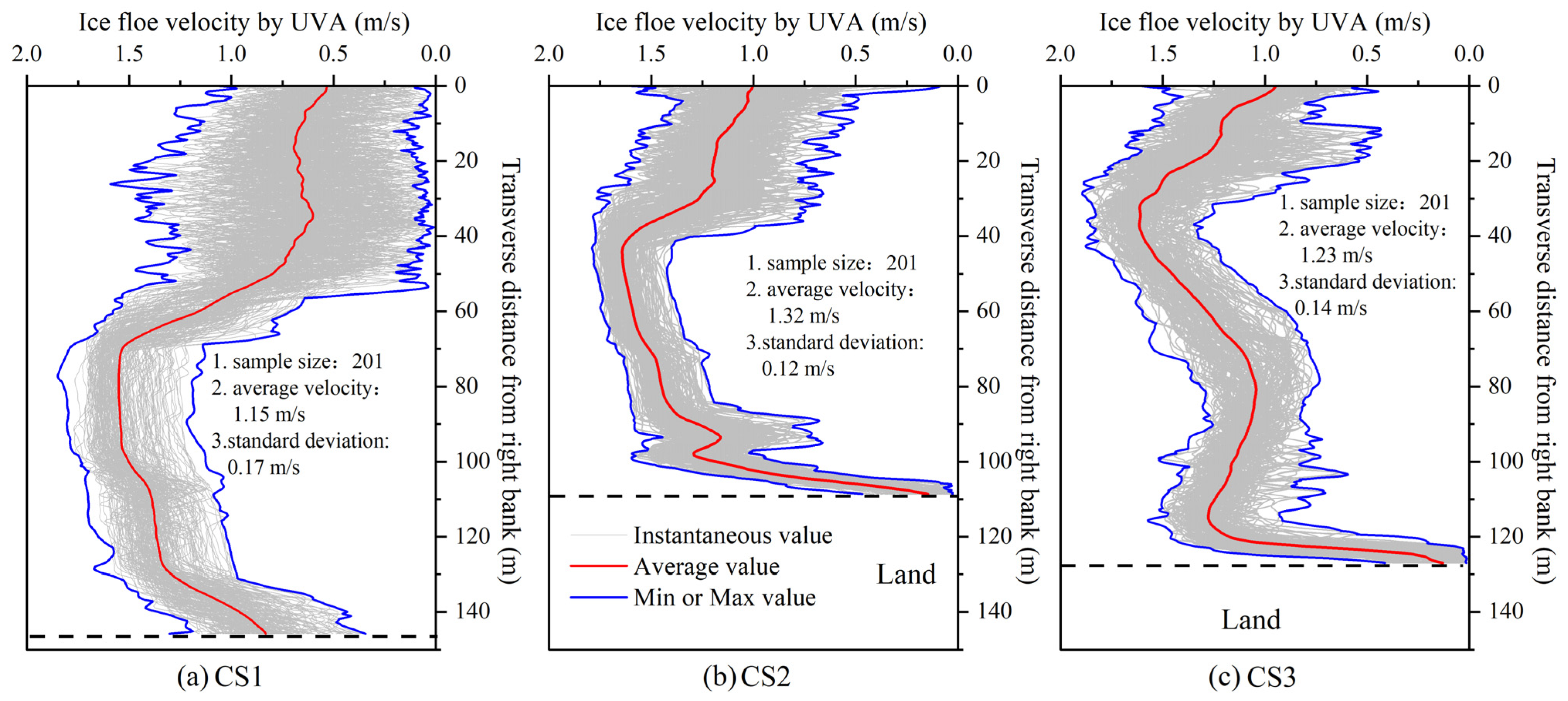
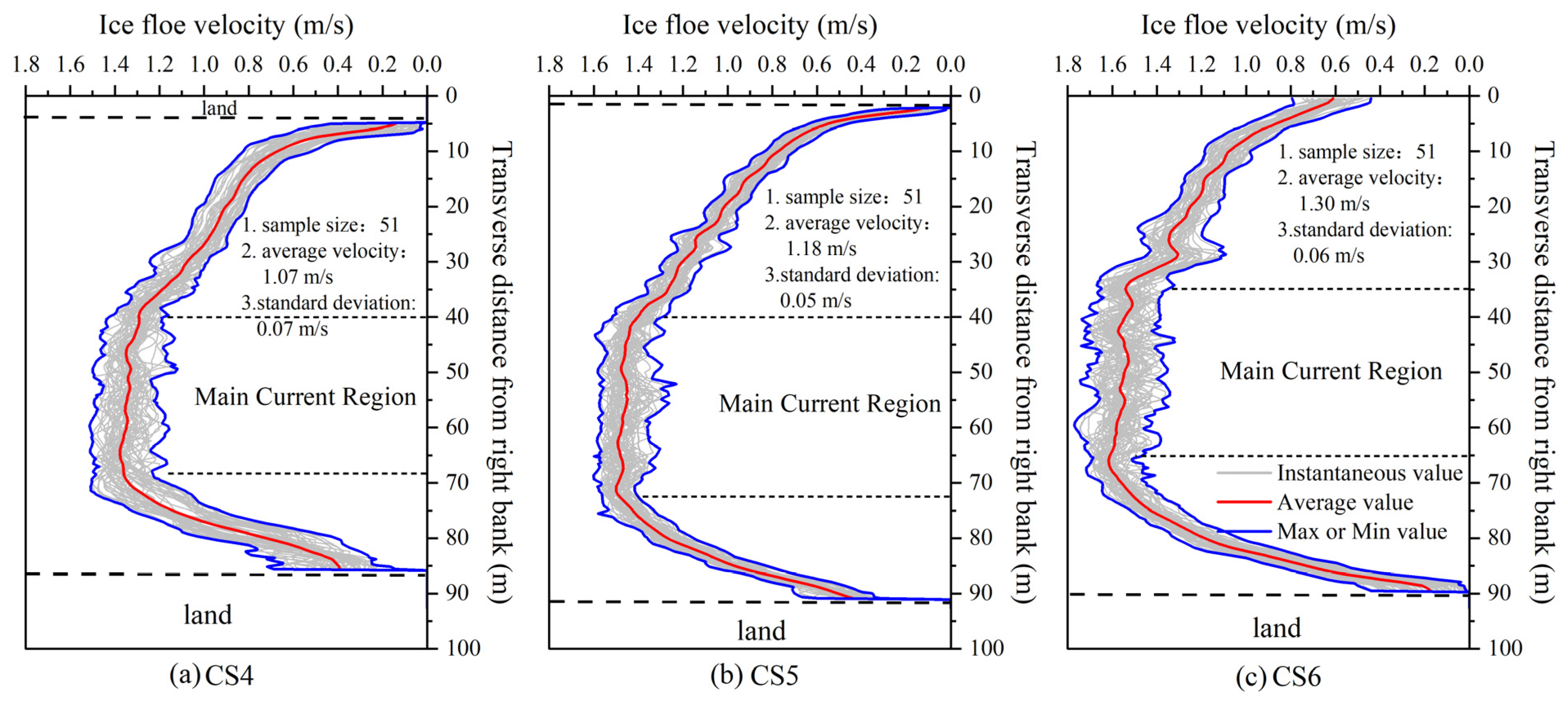
UAV vertical video imagery combined with the PIV method can capture second-scale fluctuations in drifting ice floe motion. Figure 7 and Figure 8 present typical ice floe velocity profiles for the Minjibu bend and the Xiaying straight channel, respectively. Each profile includes instantaneous velocity curves at 1 s intervals (gray lines), the mean velocity curve (red line), and the maximum and minimum velocity envelopes (blue lines).

In the bend region (Figure 7), the average velocities of the three cross-sections (CS1–CS3) are 1.15, 1.43, and 1.23 m/s respectively. The overall average velocity is 1.27 m/s. The ice floe velocity profiles at different cross-sections exhibit either single-peak or double-peak distributions. The single-peak pattern (Figure 7a) corresponds to cross-sections dominated by the mainstream flow, whereas the double-peak patterns (Figure 7b,c) mainly occur at locations influenced by the confluence of two ice floe streams or by pronounced flow bifurcation. The double-peak distributions reflect the coexistence of a primary flow and secondary flow under complex hydrodynamic conditions in the bend, rather than being caused by errors in video-based interpretation. Ice floe velocities in the mainstream zone are generally higher, ranging from approximately 1.44 to 1.67 m/s, and are associated with higher ice floe concentrations, indicating a pronounced tendency for ice floes to aggregate in high-velocity regions.

In the straight channel region (Figure 8), the average velocities of the three cross-sections (CS4–CS6) in the curve area are 1.07, 1.18, and 1.30 m/s respectively. The overall average velocity is 1.18 m/s. The ice floe velocity profiles generally exhibit a typical single-peak parabolic distribution, with the highest velocities occurring in the center of the channel and significantly lower velocities near both banks. Longitudinal comparisons show that, as the channel gradually narrows, the extent of the mainstream zone decreases, and the mean ice floe velocity declines from approximately 1.62 m/s at the upstream CS6 cross-section to about 1.38 m/s at the downstream CS4 cross-section. This phenomenon indicates that, under conditions of increasing ice floe concentration, channel narrowing does not lead to an increase in ice floe velocity; instead, enhanced crowding and interactions among ice floes suppress the overall motion of drifting ice.

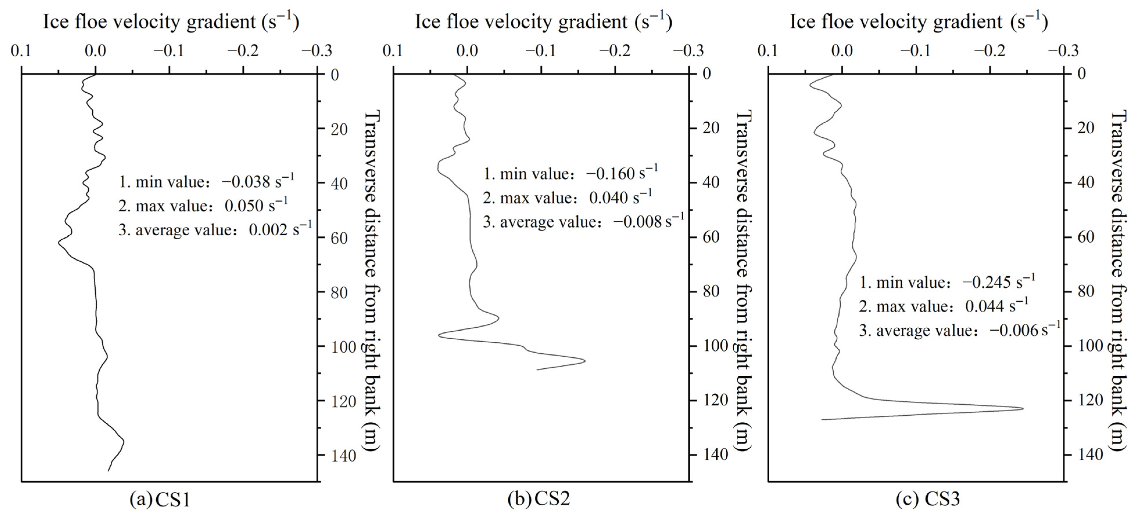
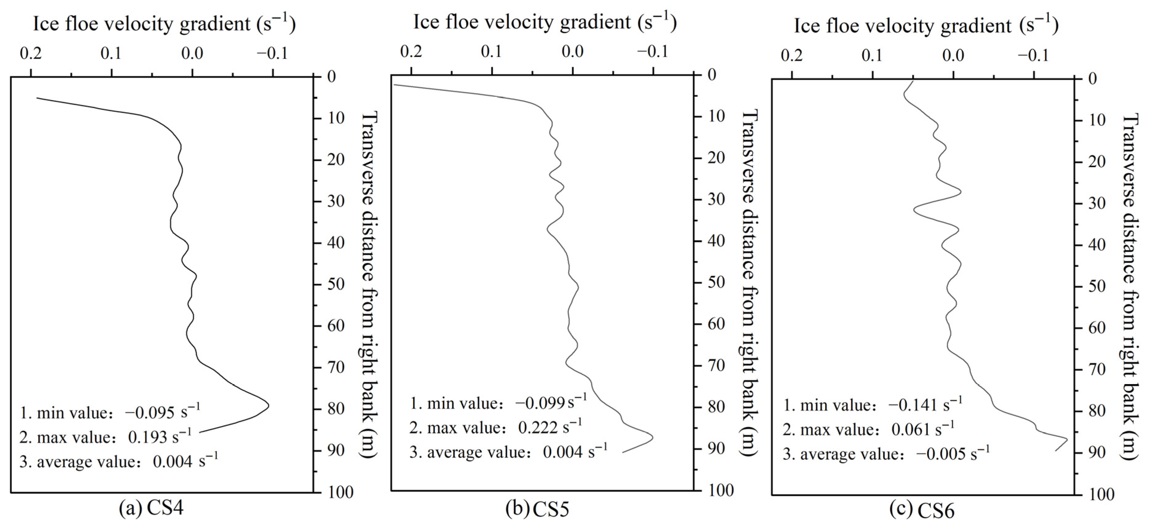
Based on the average velocity profiles across sections CS1–CS6, the lateral velocity gradient was computed using Formula (1), serving as an indicator of the transverse shear strength in the surface layer. Figure 9 shows that at the Minjibu bend, the range of velocity gradients of the three cross-sections (CS1–CS3) is −0.038–0.050 s⁻¹, −0.160–0.040 s⁻¹, and −0.245–0.044 s⁻¹, respectively. The range of overall velocity gradients is −0.245–0.050 s⁻¹. The overall amplitude of the velocity gradients in CS1 and CS2 is relatively small, while CS3 exhibits a larger gradient amplitude and stronger spatial variability, especially near the confluence of the river channel, where the peak gradient approaches −0.3 s⁻¹. These notable gradient variations suggest that the meandering effect of the river channel intensifies the transverse redistribution of momentum. In the Xiaying straight channel (Figure 10), the range of velocity gradients of the three cross-sections (CS4–CS6) is −0.095–0.193 s⁻¹, −0.099–0.222 s⁻¹, and −0.141–0.061 s⁻¹, respectively. The range of overall velocity gradients is −0.141–0.222 s⁻¹. The overall gradient distribution of CS4–CS6 is relatively smooth, but there are local gradient peaks of approximately 0.20 s⁻¹ in the right bank areas of CS4 and CS5, indicating strong local shear forces in these regions. Nevertheless, when compared to the extreme values observed in the meandering reach, the overall shear strength and spatial variability in the straight reach remain comparatively low.

Table 3. Characteristic ice floe velocities at cross-sections in the Minjibu bend and the Xiaying straight channel.

Location	Cross-Section	Region	Mean (m/s)	Variance (m/s)	Range (m/s)
Minjibu bend	CS1	Low concentration 1	0.66	0.24	1.23
		High concentration 2	1.34	0.14	0.72
	CS2	Low concentration 1	1.31	0.15	0.81
		High concentration 2	1.34	0.10	0.52
	CS3	Low concentration 1	1.39	0.15	0.80
		High concentration 2	1.12	0.13	0.68
Xiaying straight channel	CS4	Full cross-section	1.07	0.07	0.31
	CS5	Full cross-section	1.18	0.05	0.21
	CS6	Full cross-section	1.30	0.06	0.29

¹ Region from 0 to 50 m; ² region from 50 to 140 m.

presents the mean values, variances, and ranges of ice floe velocity profiles in regions with different ice floe concentrations. Further statistical analysis indicates that, in the bend region, the variance and range of instantaneous ice floe velocities in low-concentration zones are significantly larger than those in high-concentration zones. This suggests that, in sparsely distributed ice floe areas, ice floe motion is more susceptible to local disturbances, resulting in greater velocity fluctuations and lower stability of video-derived velocity estimates. In contrast, in regions with high ice floe concentration, mutual constraints among ice floes lead to more stable overall motion. In comparison, ice floe distribution in the straight channel region is relatively uniform, and the velocity variances across different cross-sections are generally smaller, indicating higher stability of the velocity estimates derived from video interpretation.

3.2. Short-Distance Translational Trajectories and Rotational Characteristics of Individual Ice Floes

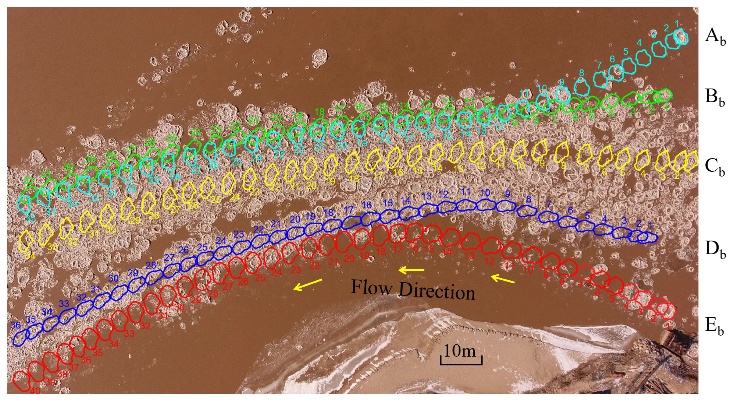
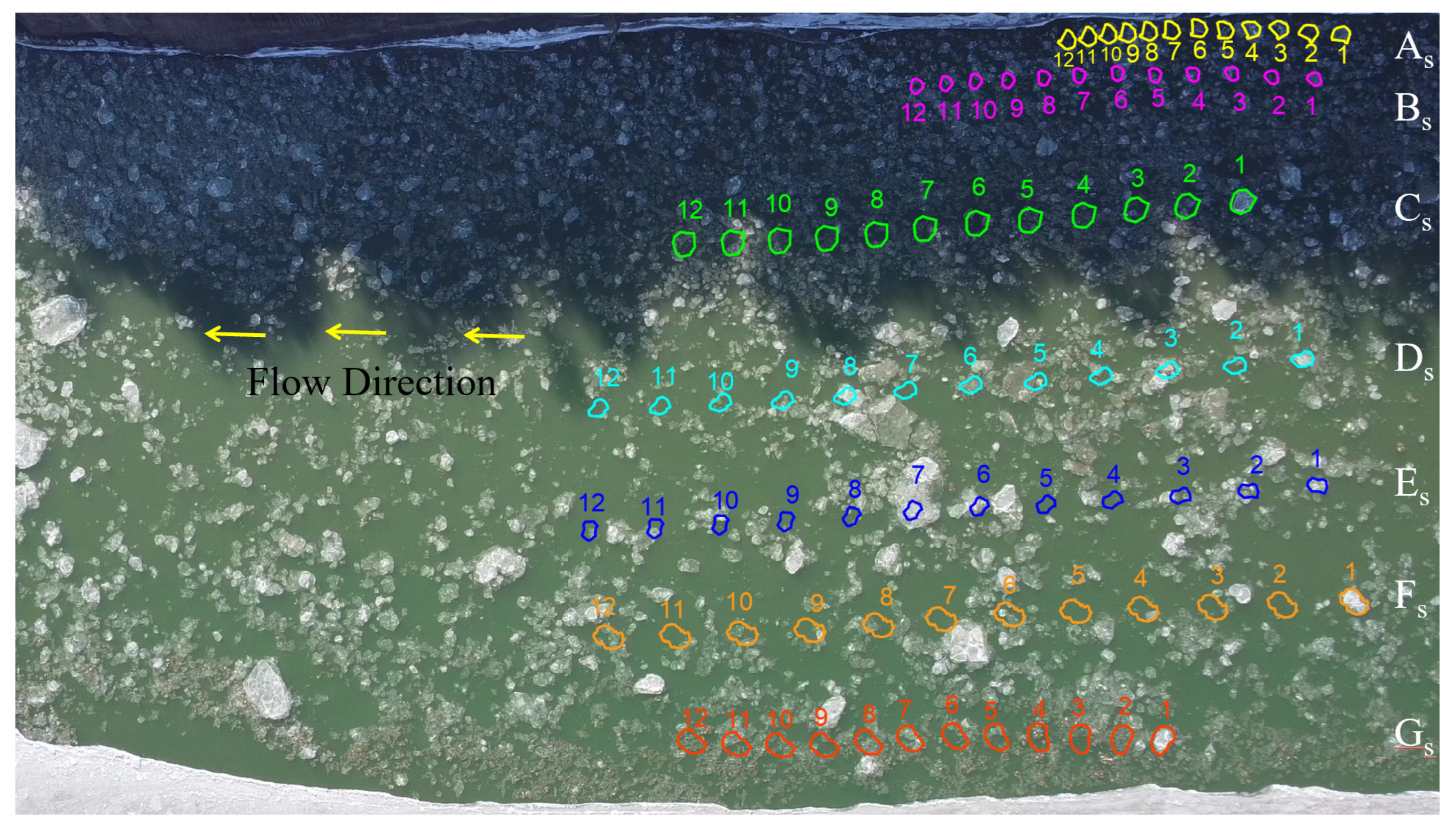
Owing to the high spatial resolution of UAV imagery, the edge features of individual ice floes can be clearly distinguished, enabling effective identification and analysis of ice floe rotation processes in video sequences. Based on UAV vertical video imagery, individual drifting ice floes at multiple representative locations in the Minjibu bend and the Xiaying straight channel were selected, and their translational trajectories (Figure 11 and Figure 12) and angular velocity (Figure 13 and Figure 14) were extracted and analyzed in detail.

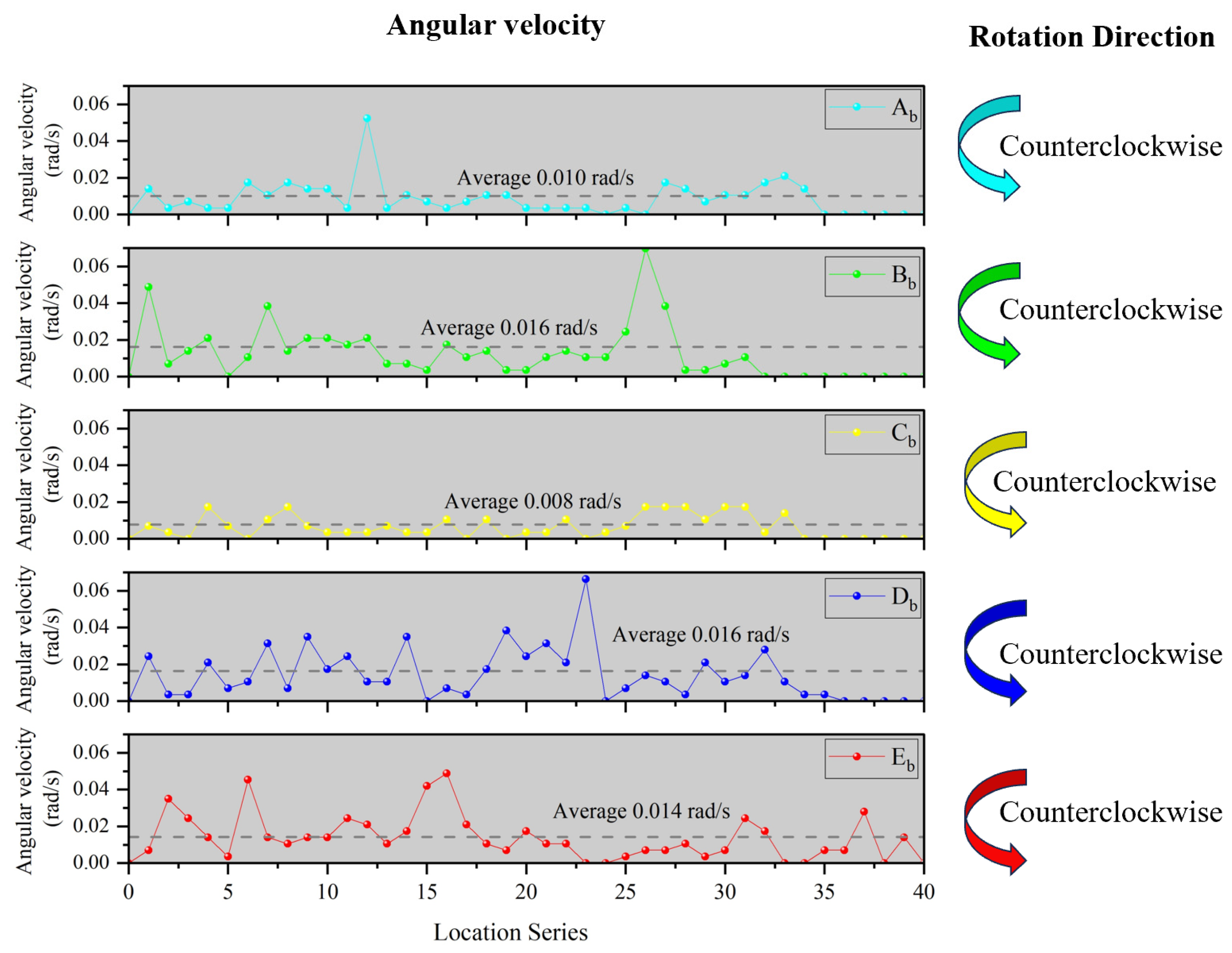
In the Minjibu bend region (Figure 11), the translational trajectories of ice floes exhibit pronounced lateral deviations. Some ice floes (${\mathrm{A}}_{\mathrm{b}} \mathrm{a}\mathrm{n}\mathrm{d} {\mathrm{E}}_{\mathrm{b}}$) show a tendency to migrate from marginal areas toward the mainstream zone during their motion, but do not enter the mainstream core. Other ice floes (${\mathrm{B}}_{\mathrm{b}} \mathrm{a}\mathrm{n}\mathrm{d}$ ${\mathrm{D}}_{\mathrm{b}}$) move persistently along the edge of the mainstream, whereas ice floes located within the mainstream core (${\mathrm{C}}_{\mathrm{b}}$) display relatively stable trajectories with limited lateral displacement. These results indicate that the translational trajectories of ice floes in bends are not solely controlled by the velocity distribution of the flow but are jointly influenced by ice–ice interactions and local flow field structures.

In the Xiaying straight channel region (Figure 12), the trajectories of individual ice floes are generally parallel, with almost no evident lateral convergence or divergence among ice floes. Ice floes in the central part of the channel exhibit higher velocities, whereas those near the banks move more slowly. The translational velocity characteristics are highly consistent with the lateral velocity distribution of the straight channel flow, reflecting relatively simple and stable hydrodynamic conditions.

To better quantify rotational dynamics, ice floe rotation was converted from cumulative rotation angle to angular velocity (rad/s) based on the corresponding time interval of 5 s. Ice floe rotational characteristics show significant differences between the bend and straight channel regions. In the Minjibu bend (Figure 13), all tracked individual ice floes rotate counterclockwise during their motion, with angular velocity generally ranging from 0.003 to 0.070 rad/s and mean angular velocity ranging from approximately 0.008 rad/s to 0.016 rad/s. In the mainstream core, where ice floe concentration is relatively high, mutual compression among ice floes limits rotation, resulting in smaller rotational angles. In contrast, at the edges of the mainstream and at tributary confluence zones, ice floes are more prone to collisions, leading to multiple rotation events with angles exceeding 0.035 rad/s. These results indicate that ice floe rotation is primarily triggered by ice–ice collisions and locally non-uniform shear, rather than being determined solely by flow velocity magnitude.

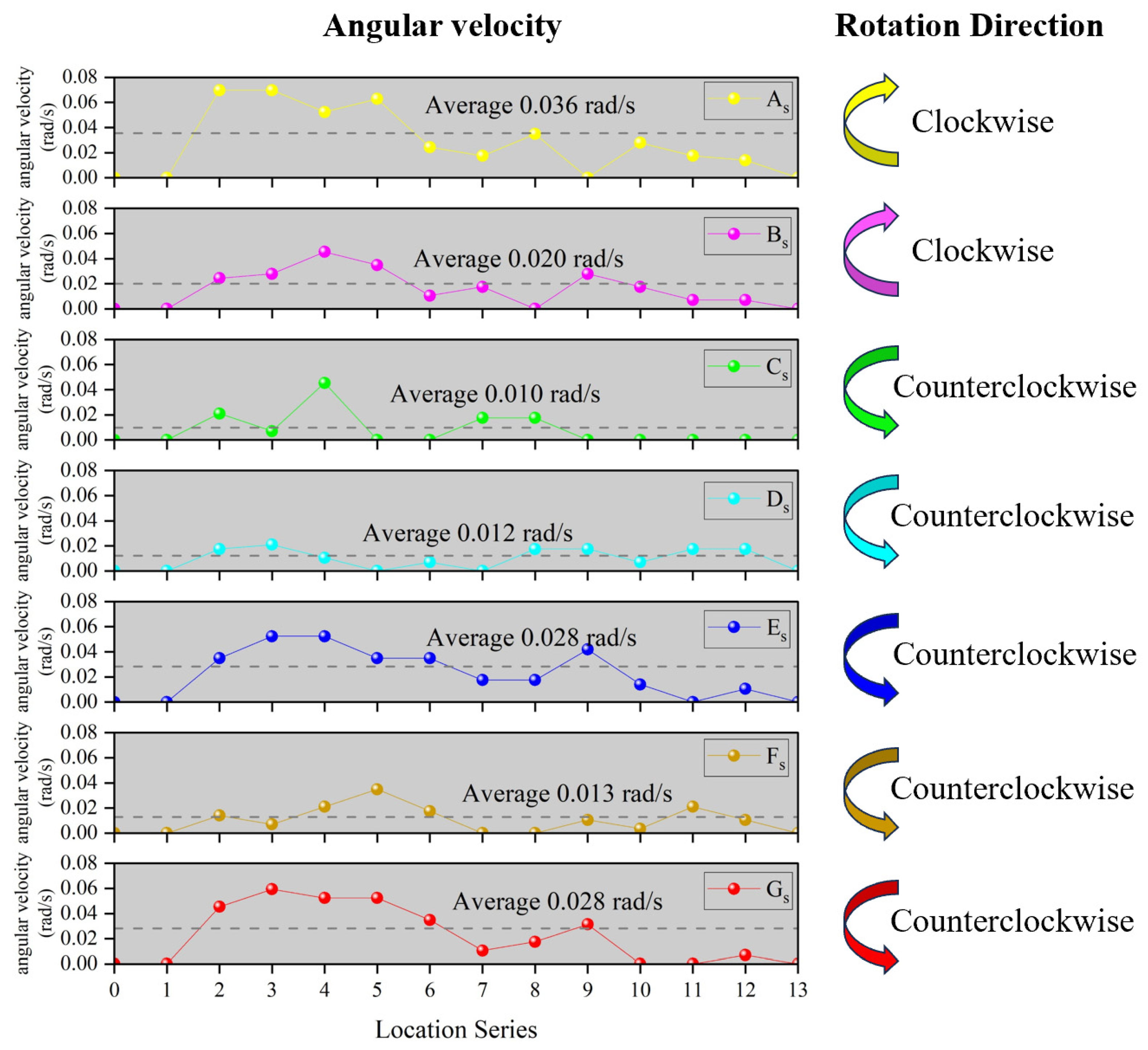
In the Xiaying straight channel region (Figure 14), ice floe rotation directions exhibit distinct spatial differences. Ice floes near the right bank (${\mathrm{A}}_{\mathrm{s}} \mathrm{a}\mathrm{n}\mathrm{d}$ ${\mathrm{B}}_{\mathrm{s}}$) predominantly rotate clockwise, whereas those in the channel center and near the left bank (${\mathrm{C}}_{\mathrm{s}}$~${\mathrm{G}}_{\mathrm{s}}$) mainly rotate counterclockwise. Overall, angular velocity in the straight channel ranges from 0.003 to 0.070 rad/s, with a mean angular velocity of approximately 0.010 rad/s to 0.036 rad/s. Ice floes near the banks experience more pronounced rotational directions and amplitudes due to bank-induced resistance and asymmetric drag, whereas ice floes in the channel center generally exhibit smaller rotations. However, changes in rotation direction can still occur when local ice floe concentration decreases or velocity gradients increase.

3.3. Long-Distance Motion Characteristics of Drifting Ice Floes

By tracking drifting ice floes using throw-and-drop GPS devices, the long-distance motion trajectories, durations, and velocity characteristics of ice floes at the kilometer scale were obtained. The GPS tracking results effectively compensate for the limited spatial coverage of UAV video observations, enabling complete characterization of the drifting ice floe motion process from short-distance local movement to long-distance overall transport.

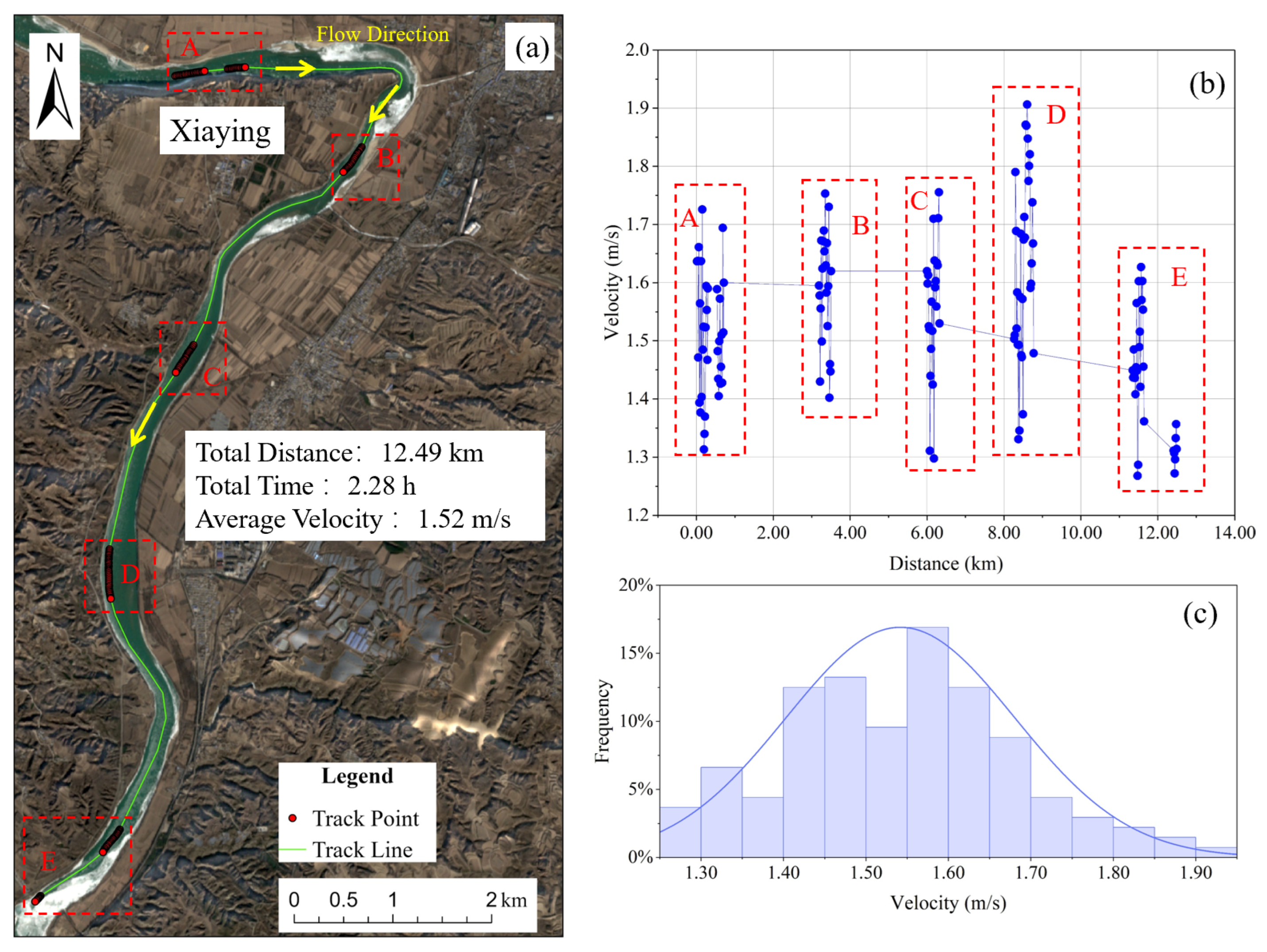
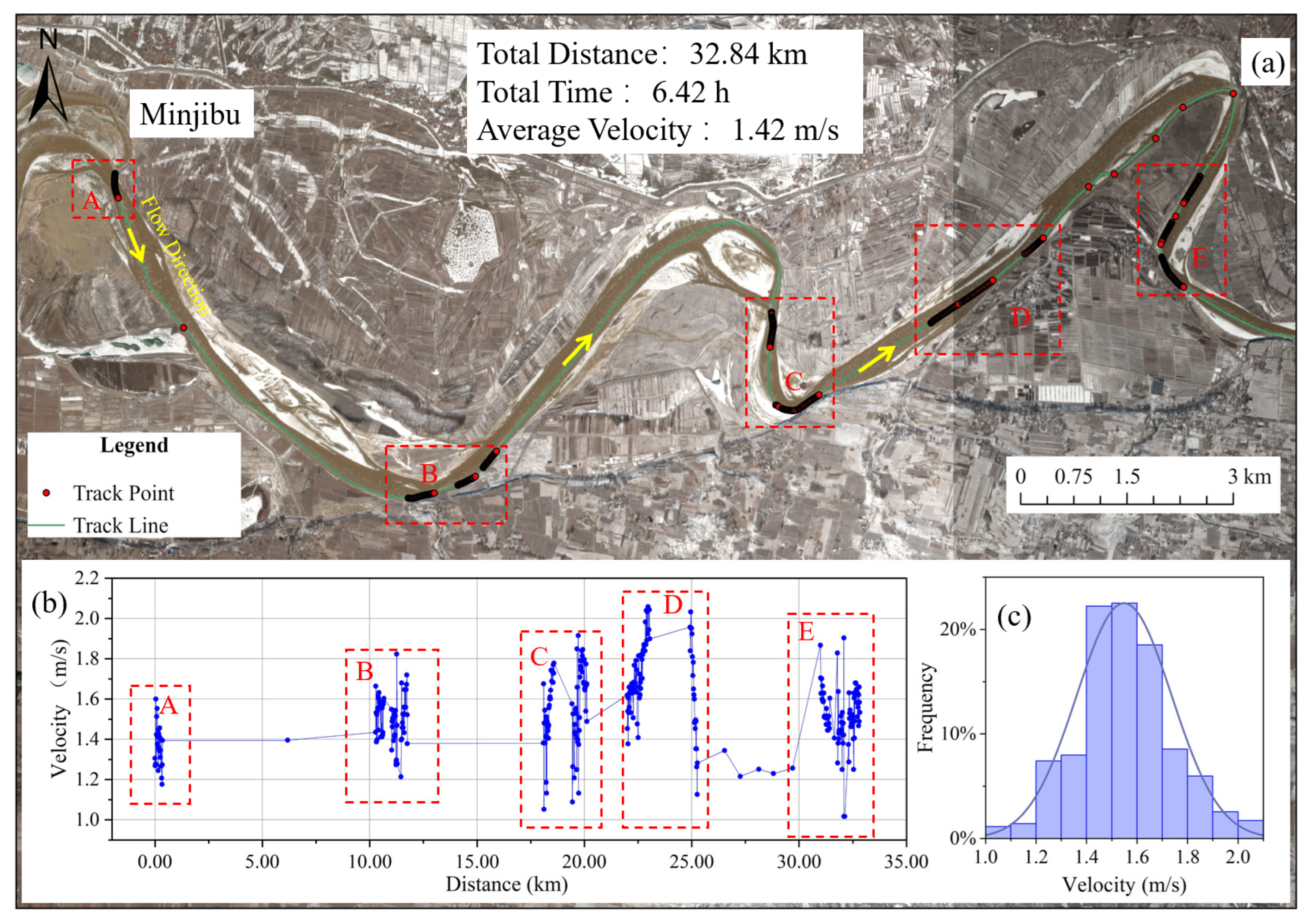
In the Minjibu bend region (Figure 15), the GPS-tracked ice floe traveled a cumulative distance of 32.84 km during the observation period, with a total travel time of 6.42 h, corresponding to a mean velocity of 1.42 m/s. In the Xiaying straight channel region (Figure 16), the ice floe traveled a total distance of 12.49 km over 2.28 h, yielding a mean velocity of 1.52 m/s.

At both experimental sites, the ice floe trajectories obtained from GPS exhibit temporal discontinuity and spatially segmented distributions. Based on the spatial displacement and time interval between adjacent valid trajectory points, the instantaneous velocities of ice floes were calculated. The results show that ice floe instantaneous velocities vary continuously throughout the motion process rather than remaining constant. In the Xiaying straight channel region, instantaneous velocities range from 1.27 to 1.91 m/s, whereas in the Minjibu bend region, instantaneous velocities range from 1.02 to 2.06 m/s, indicating larger velocity fluctuations in the bend region. Velocity distribution histograms further show that, despite these fluctuations, the velocity distributions are highly concentrated: ice floe velocities in the Minjibu bend region are mainly concentrated in the range of 1.40–1.60 m/s, while those in the Xiaying straight channel region are primarily concentrated between 1.55 and 1.60 m/s.

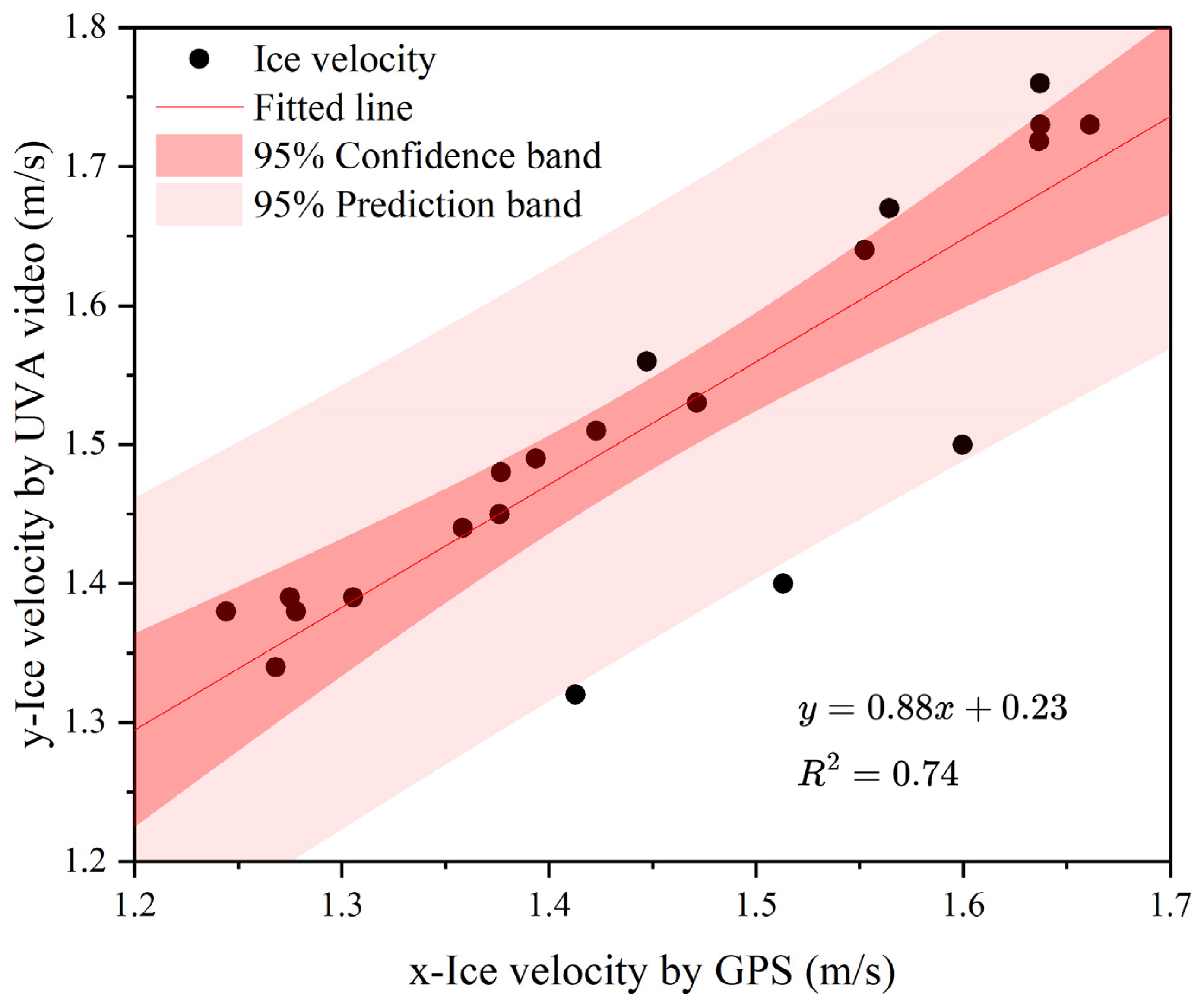
To verify the reliability of ice floe velocities derived from UAV video, a comparative analysis was conducted between ice floe velocities obtained from GPS tracking and those derived from UAV video interpretation (

Table 4. Velocity errors between ice floe velocities derived from GPS tracking and UAV video interpretation.

Location	Serial Number	Velocity by GPS (m/s)	Velocity by Drone Video (m/s)	Absolute Error (m/s)
Minjibu	1	1.31	1.39	0.08
	2	1.27	1.34	0.07
	3	1.28	1.38	0.10
	4	1.60	1.5	0.10
	5	1.27	1.39	0.12
	6	1.42	1.51	0.09
	7	1.51	1.4	0.11
	8	1.55	1.64	0.09
	9	1.38	1.45	0.07
	10	1.41	1.32	0.09
	11	1.36	1.44	0.08
	12	1.24	1.38	0.14
	13	1.45	1.56	0.11
Xiaying	14	1.64	1.72	0.08
	15	1.64	1.73	0.09
	16	1.47	1.53	0.06
	17	1.66	1.73	0.07
	18	1.39	1.49	0.10
	19	1.56	1.67	0.11
	20	1.38	1.48	0.10
	21	1.64	1.76	0.12
Mean absolute error				0.10

and Figure 17). The regression between the speed obtained by the drone and the speed obtained by GPS shows a slope of 0.88, with R² = 0.74. The underestimation rate of the unmanned aerial vehicle measurement system is about 12%. This deviation may be caused by the slight shaking of the drone affected by wind speed, the average instantaneous velocity within 10 s of the video, and the inherent spatial smoothing in the PIV algorithm. There are three points in Figure 17 that deviate significantly from the regression line, which may be caused by short-term collision deformation of floating ice resulting in GPS position changes on the ice surface. The average absolute error between the two methods is 0.10 m/s, corresponding to less than 8% of the observed velocity range. For on-site river ice monitoring applications, the overall error is acceptable.

By integrating the long-distance GPS tracking results with UAV video interpretation results, it can be concluded that GPS technology is effective for characterizing the overall transport of drifting ice floes at the kilometer scale, whereas UAV video is better suited for capturing fine-scale velocity fields and rotational characteristics at local scales. The combination of these two observation techniques enables multi-scale characterization of drifting ice floe motion from short-distance detailed structures to long-distance overall transport processes.

4. Discussion

4.1. Advantages and Remote Sensing Implications of UAV–GPS Joint Observations

This study combines UVA video and GPS tracking technology to obtain river ice motion parameters. It obtains not only local river ice motion velocity, lateral velocity gradient, single floating ice rotation angle, rotation direction, and rotation angular velocity, but also long-distance floating ice motion trajectory, transportation distance, transportation time, and average transportation speed.

Compared with previous methods of observing river ice movement, shore-based camera observation technology has some advantages. However, it is limited by the distortion of floating ice images and limited field of view, making it difficult to accurately extract details such as floating ice rotation. The existing free satellite remote sensing observation technology is limited by low temporal and spatial resolution, and cannot distinguish individual floating ice and track its movement. In high-latitude regions, the overlap of multiple satellite sources is high, which can improve the temporal resolution of the intersection and thus observe the movement of floating ice. Altena and Kääb [18] used the 196.83 s time difference between Sentinel-2 and PROBA-V satellites to calculate the velocity of ice floes in the Lena River in the Arctic region. They also pointed out that the ideal time interval between the two images should be controlled at 30 s. Unmanned aerial vehicle observation technology can obtain high-definition ice floe motion videos. Wang et al. [36] mainly studied the application of the UAV-SIFT algorithm to interpret the velocity of ice floes in the Heilongjiang River, but lacked interpretation of the translational and rotational processes of individual ice floes. Due to battery limitations in winter, drones have a flight time of approximately 20–40 min and are unable to track the movement of floating ice over long distances. GPS, due to its low power consumption, can be applied for long-distance tracking of floating ice transport. The self-power of the GPS device used in this study can be used for continuous monitoring for 10–15 days, and the monitored positioning data are uploaded in real-time to the cloud platform. Even if the GPS is lost or not recovered, the positioning data can still be downloaded.

The joint remote sensing observation method can describe the dynamic behavior of floating ice from local movement to long-distance transportation, enhancing the integrated monitoring capability of river ice, air space, and ground. This observation method was tested under two typical terrain conditions of the Yellow River (curved channel and straight channel) with good results. Drone observation of floating ice movement is relatively mature, and one can proficiently operate the drone to shoot videos vertically. Due to the negative temperature during winter, the flight time of drones will be shortened. Previously, we conducted GPS tracking of floating ice technology tests at 10 locations within 840 km of the Inner Mongolia section of the Yellow River, and the results were good. The caveat of GPS technology lies in the inability of unmanned aerial vehicles to accurately reach the surface of floating ice when deploying the GPS. The plastic bucket that wraps the GPS is not tightly sealed, and the floating ice can hit and squash the plastic bucket, causing the GPS to fail due to water ingress. When the GPS enters the frozen area, it is can easily be submerged under the ice and lose signal. Although this joint observation technology is only tested in the Minjibu bend and Xiaying straight river channel, it is also applicable to other frozen sections of the Yellow River.

4.2. Estimation of Ice Rotation Accuracy and Influencing Factors

This study utilizes manual contouring of drone videos to track ice rotation and estimates the accuracy of manual rotation tracking based on image resolution and frame rate. For video image spatial resolution (~0.05 m) and a 5 s time interval, the minimum recognizable angle is about 1° (0.017 rad), and the average rotation error after 5 s is 0.0034 rad/s. The angular velocity range of the five ice blocks in the curved area is 0.003 to 0.070 rad/s, and the overall average angular velocity ranges from 0.008 to 0.016 rad/s. The angular velocities of the seven ice blocks in the straight river range from 0.003 to 0.070 rad/s, with an overall average angular velocity of 0.010 rad/s to 0.036 rad/s. The relative uncertainty of most tracked floating ice is usually less than 10–20%. The uncertainty of the minimum angular velocity identified in this study is high, but the overall rotation trend and shear relationship trend are good. In the future, the minimum recognizable angle and rotation time interval can be increased to reduce rotation errors.

Ice rotation is affected by lateral velocity gradient, ice collision, and bend curvature. This study compared the rotational angular velocity of ice cubes (Figure 13 and Figure 14) with the lateral velocity gradient (Figure 9 and Figure 10). The results show that ice cubes with larger velocity gradients exhibited higher rotational angular velocities, and the rotational velocity of ice cubes was positively correlated with the absolute value of the velocity gradient. This is because the lateral velocity gradient generates varied resistance to floating ice, causing the ice to rotate. Video observations indicate that instances of relatively high instantaneous angular velocities often coincide with the collision of floating ice, suggesting that collisions may produce short-term rotational fluctuations, which are sporadic and not proportional to the magnitude of the angular velocity. The curvature of a bend is an indirect influencing factor which enhances lateral shear by changing the water level difference between the inside and outside of the bend. However, compared to collision effects, the impact is relatively small. Overall analysis shows that under on-site observation conditions, the lateral velocity gradient is the dominant factor, collision is the instantaneous disturbance factor, and the curvature of the river channel is indirectly controlled through shear enhancement.

Although the number of rotating floating ice blocks tracked is limited (five in bends and seven in straight lines), the selected floating ice covers multiple regional locations, including those distributed in river boundary areas, main river areas, tributary confluence areas, high-density areas, and low-density areas, to identify the physical factors affecting ice rotation. In the future, multiple floating ice blocks can be selected in different regions to attempt to establish a statistical relationship between the rotational angular velocity of floating ice and the influencing factor velocity.

To quantitatively explore the relationship between rotation and shear, we conducted a comparative analysis between the mean angular velocity of floating ice (Figure 13 and Figure 14) and the corresponding lateral velocity gradient at each cross-section (Figure 9 and Figure 10). The results indicate that ice blocks at locations with larger velocity gradients generally exhibit higher rotational angular velocities. The direction of ice block rotation correlates with the sign of the velocity gradient, with negative velocity gradients in curved channels indicating counterclockwise rotation. Conversely, in straight channels, ice blocks at sites with positive velocity gradients rotate clockwise, whereas those at sites with negative velocity gradients rotate counterclockwise. Furthermore, a positive correlation exists between the rotational speed of ice blocks and the absolute magnitude of the local velocity gradient, thereby providing quantitative evidence that lateral water flow shear constitutes one of the primary physical mechanisms propelling river ice rotation.

4.3. Limitations and Future Research Perspectives

The two locations selected in this paper represent typical bend and straight channel morphologies commonly found in the upper and middle reaches of the Yellow River under seasonal freeze-up conditions. Although these river sections exhibit typical hydraulic and geometric characteristics, the research findings may not be directly applicable to braided river sections, sections subject to strong regulation, or extreme ice jam scenarios.

The on-site experiment was conducted during the freeze-up period of the Yellow River, with a floating ice density between 50% and 90% and a flow velocity between 1.44 and 1.67 m per second. Although the sample size tracked by GPS is limited, the floating ice velocity, shear strength, and rotation relationship under both river channel shapes have been observed on site within this concentration and flow velocity range. According to Li et al.’s [40] on-site observations of the scale of floating ice during the freeze-up and break-up periods of the Yellow River in Inner Mongolia, the average diameters of the floating ice blocks were 3.36 m and 2.30 m, respectively. The difference in scale between the two periods is not significant, and this study can also be applied to the opening period, but not to extreme ice blockage and dam situations.

The nominal horizontal positioning accuracy of GPS devices is approximately 5 m (Table 2). Assuming that this maximum positioning error is independent between consecutive observations, the theoretical upper limit of velocity uncertainty can reach approximately 0.7 m/s. However, the error estimation is upper-bounded. In practical applications, the actual positioning error is usually smaller than the nominal maximum value and exhibits temporal correlation between consecutive measurements. This study employed river boundary constraints and trajectory smoothness checks to eliminate abnormal positioning points, and selected continuous trajectory segments for velocity estimation. The results indicated that the uncertainty in propagation velocity was significantly lower than the theoretical maximum when compared to the velocity obtained from drones, with an average absolute error of 0.10 m/s. The consistency between GPS and UVA velocity estimation results suggests that GPS positioning errors have a minor impact on the analysis of long-distance ice floe movement.

Automated tracking of individual ice floe is a key focus of future research. Under the complex visual conditions of the Yellow River ice, including ice water with sand, the low contrast of ice water, and the high density of ice floe collision deformation and overlap, automated tracking still faces significant challenges. Zhang [32,33] mainly applies semantic segmentation techniques to classify the ice water bank images of the Yellow River, and these methods have shown effectiveness in large-scale ice water image classification and static image segmentation. However, although existing image tracking algorithms can provide the overall translational and rotational trends of floating ice, they still cannot achieve automatic tracking of the motion details of a single Yellow River floating ice block due to its unclear boundaries, variable shapes, and complex textures. Therefore, this study first used the method of manually tracking individual floating ice to obtain on-site floating ice rotation data and quantitatively analyze the main physical influencing factors of floating ice. In the future, two key issues will be focused on in the automated tracking of individual Yellow River floating ice blocks: firstly, the dynamic and accurate identification of boundaries during the movement of a single floating ice block; secondly, tracking the rotational angular velocity based on multiple feature points of ice floe. Multiple algorithms and models including DeepLab, SegNet, U-Net, Mask R-CNN, YOLO, and LLM can be used in combination.

5. Conclusions

During the winter of 2024–2025, field experiments were conducted in the Minjibu bend of the upper Yellow River and the Xiaying straight reach of the middle Yellow River under ice concentrations of 50–90%. By integrating UAV vertical video imagery with throw-and-drop GPS tracking technology, both local ice motion characteristics and long-distance drift behavior were quantified. The obtained on-site motion parameters are of great value for the physical and numerical simulation of river ice movement processes, as well as for the monitoring and warning of river ice hazards. The main conclusions are as follows:

• Based on UAV vertical video imagery and the PIV method, the spatial distribution characteristics of ice floe velocity fields and cross-sectional velocities in bend and straight channel reaches were obtained. In bend and straight river channels, the average speeds of floating ice are 1.27 m/s and 1.18 m/s, respectively, with velocity gradient ranges of −0.245 to 0.050 s⁻¹ and −0.141 to 0.222 s⁻¹, respectively.
• Leveraging the high spatial resolution of UAV imagery, translational trajectories and rotational characteristics of individual drifting ice floes were extracted. In bend and straight river channels, the rotational angular velocity ranges are 0.008 rad/s to 0.016 rad/s and 0.010 rad/s to 0.036 rad/s, respectively. The angular velocity of ice cube rotation exhibits a strong positive correlation with the lateral velocity gradient, and the direction of ice cube rotation is correlated with the sign of the velocity gradient.
• A joint remote sensing observation approach combining high-resolution short-distance UAV observations and long-distance GPS tracking was proposed, enabling continuous characterization of drifting ice floe motion from local fine-scale structures to kilometer-scale overall transport processes. The average error between the ice floe speed obtained through GPS tracking and the speed derived from drone video interpretation is 0.10 m/s, verifying the reliability of drone-based ice floe speed inversion.

References

1. Shen, H.T. Mathematical modeling of river ice processes. Cold Reg. Sci. Technol. 2010, 62, 3–13. [Google Scholar] [CrossRef] [Scilit]
2. Liu, B.; Ji, H.L.; Zhai, Y.G.; Luo, H.C. Estimation of river ice thickness in the Shisifenzi reach of the Yellow River with remote sensing and air temperature data. IEEE J. Sel. Top. Appl. Earth Observ. Remote Sens. 2023, 16, 5645–5659. [Google Scholar] [CrossRef] [Scilit]
3. Su, H.; Xu, W.; Li, H.; Yang, Q.; Chen, Y.; Wu, Z.; Paoletti, M.E.; Du, Q. River ice monitoring from optical and SAR remote sensing perspective: Advances, challenges and opportunities. Innov. Geos. 2025, 3, 100152. [Google Scholar] [CrossRef] [Scilit]
4. Pavelsky, T.M.; Smith, L.C. Spatial and Temporal Patterns in Arctic River Ice Breakup Observed with MODIS and AVHRR Time series. Remote Sens. Environ. 2004, 93, 328–338. [Google Scholar] [CrossRef] [Scilit]
5. Li, H.J.; Li, H.Y.; Wang, J.; Hao, X.H. Revealing the River Ice Phenology on the Tibetan Plateau Using Sentinel-2 and Landsat 8 Overlapping Orbit Imagery. J. Hydrol. 2023, 619, 129285. [Google Scholar] [CrossRef] [Scilit]
6. Beaton, A.; Whaley, R.; Corston, K.; Kenny, F. Identifying Historic River Ice Breakup Timing Using MODIS and Google Earth Engine in Support of Operational Flood Monitoring in Northern Ontario. Remote Sens. Environ. 2019, 224, 352–364. [Google Scholar] [CrossRef] [Scilit]
7. Zhang, X.; Xia, H.; Sheng, Y. Monitoring River Ice in the Northern Section of Yellow River Using Sentinel-1/2 Images. IEEE J.-STARS 2004, 17, 13232–13243. [Google Scholar] [CrossRef] [Scilit]
8. Wei, C.X.; Li, H.X.; Chen, L.; Zhou, H.H.; Taukebayev, O.; Wu, W.C. River Ice Fine-Grained Segmentation: A GF-2 Satellite Image Dataset and Deep Learning Benchmark. IEEE Trans. Geosci. Electron. 2025, 63, 5407115. [Google Scholar] [CrossRef] [Scilit]
9. Stonevicius, E.; Uselis, G.; Grendaite, D. Ice Detection with Sentinel-1 SAR Backscatter Threshold in Long Sections of Temperate Climate Rivers. Remote Sens. 2022, 14, 1627. [Google Scholar] [CrossRef] [Scilit]
10. Weber, F.; Nixon, D.; Hurley, J. Semi-automated classification of river ice types on the Peace River using RADARSAT-1 synthetic aperture radar (SAR) imagery. Can. J. Civ. Eng. 2003, 30, 11–27. [Google Scholar] [CrossRef] [Scilit]
11. Zhang, F.; Li, Z.Q.; Lindenschmidt, K.-E. Potential of RADARSAT-2 to Improve Ice Thickness Calculations in Remote, Poorly Accessible Areas: A Case Study on the Slave River, Canada. Can. J. Remote Sens. 2019, 45, 234–245. [Google Scholar] [CrossRef] [Scilit]
12. Das, A.; Sagin, J.; Van Der Sanden, J.; Evans, E.; McKay, H.; Lindenschmidt, K.-E. Monitoring the Freeze-up and Ice Cover Progression of the Slave River. Can. J. Civ. Eng. 2015, 42, 609–621. [Google Scholar] [CrossRef] [Scilit]
13. Chaouch, N.; Temimi, M.; Romanov, P.; Cabrera, R.; McKillop, G.; Khanbilvardi, R. An Automated Algorithm for River Ice Monitoring over the Susquehanna River Using the MODIS Data. Hydrol. Process. 2014, 28, 62–73. [Google Scholar] [CrossRef] [Scilit]
14. Sobiech, J.; Dierking, W. Observing Lake- and River-Ice Decay with SAR: Advantages and Limitations of the Unsupervised k-Means Classification Approach. Ann. Glaciol. 2013, 54, 65–72. [Google Scholar] [CrossRef] [Scilit]
15. Palomaki, R.T.; Sproles, E.A. Quantifying the Effect of River Ice Surface Roughness on Sentinel-1 SAR Backscatter. Remote Sens. 2022, 14, 5644. [Google Scholar] [CrossRef] [Scilit]
16. Yang, X.; Pavelsky, T.M.; Allen, G.H. The past and future of global river ice. Nature 2020, 577, 69–73. [Google Scholar] [CrossRef] [Scilit]
17. Li, H.J.; Li, H.Y.; Wang, J.; Hao, X.H. Monitoring high-altitude river ice distribution at the basin scale in the northeastern Tibetan Plateau from a Landsat time-series spanning 1999–2018. Remote Sens. Environ. 2020, 247, 111915. [Google Scholar] [CrossRef] [Scilit]
18. Altena, B.; Kääb, A. Quantifying River ice movement through a combination of European satellite monitoring services. Int. J. Appl. Earth Obs. Geoinf. 2021, 98, 102315. [Google Scholar] [CrossRef] [Scilit]
19. Bourgault, D. Shore-based photogrammetry of river ice. Can. J. Civ. Eng. 2008, 35, 80–86. [Google Scholar] [CrossRef] [Scilit]
20. Pei, C.K.; She, Y.T.; Loewen, M. Deep learning-based river surface ice quantification using a distant and oblique-viewed public camera. Cold Reg. Sci. Technol. 2023, 206, 103736. [Google Scholar] [CrossRef] [Scilit]
21. Deng, Y.; Li, C.J.; Li, Z.J.; Zhang, B.S. Dynamic and full-time acquisition technology and method of ice data of Yellow River. Sensors 2021, 22, 176. [Google Scholar] [CrossRef] [Scilit]
22. Daigle, A.; Bérubé, F.; Bergeron, N.; Matte, P. A methodology based on Particle image velocimetry for river ice velocity measurement. Cold Reg. Sci. Technol. 2013, 89, 36–47. [Google Scholar] [CrossRef] [Scilit]
23. Wang, H.B.; Wang, G.H.; Tang, X.M.; Li, C.H. Yellow River icicle hazard dynamic monitoring using UAV aerial remote sensing technology. IOP Conf. Ser. Earth Environ. Sci. 2014, 18, 012043. [Google Scholar] [CrossRef] [Scilit]
24. Alfredsen, K.; Haas, C.; Tuhtan, J.A.; Zinke, P. Brief communication: Mapping River ice using drones and structure from motion. Cryosphere 2018, 12, 627–633. [Google Scholar] [CrossRef] [Scilit]
25. Alfredsen, K.; Juarez, A. Modelling stranded river ice using LIDAR and drone-based models. In Proceedings of the 25th IAHR International Symposium on Ice, Trondheim, Norway, 23–25 November 2020. [Google Scholar]
26. Li, C.J.; Li, Z.J.; Huang, W.F.; Zhang, B.S.; Deng, Y.; Li, G.Y. Morphology dynamics of ice cover in a river bend revealed by the UAV-GPR and sentinel-2. Remote Sens. 2023, 15, 3180. [Google Scholar] [CrossRef] [Scilit]
27. Meng, X.; Zhu, Z.; Liu, H.; Lian, Y.; Lu, H.; Wang, Y.; Shi, R.; Spencer, B.F. A drone-borne GPR system for lake and river ice thickness monitoring. Water Resour. Res. 2025, 61, e2025WR040290. [Google Scholar] [CrossRef] [Scilit]
28. Bai, X.; Wang, L.; Luo, X.; Mi, H.; Chen, H.; Liu, L.; Ji, M.; Gao, Y. A layer tracking method for ice thickness detection based on GPR mounted on the UAV. In Proceedings of the 4th International Conference on Imaging, Signal Processing and Communications (ICISPC), Kumamoto, Japan, 23–25 October 2020. [Google Scholar]
29. Kalke, H.; Loewen, M. Support vector machine learning applied to digital images of river ice conditions. Cold Reg. Sci. Technol. 2018, 155, 225–236. [Google Scholar] [CrossRef] [Scilit]
30. Singh, A.; Kalke, H.; Loewen, M.; Ray, N. River ice segmentation with deep learning. IEEE Trans. Geosci. Remote Sens. 2020, 58, 7570–7579. [Google Scholar] [CrossRef] [Scilit]
31. Ansari, S.; Rennie, C.D.; Clark, S.P.; Seidou, O. IceMaskNet: River ice detection and characterization using deep learning algorithms applied to aerial photography. Cold Reg. Sci. Technol. 2021, 189, 103324. [Google Scholar] [CrossRef] [Scilit]
32. Zhang, X.W.; Jin, J.J.; Lan, Z.; Li, C.J.; Fan, M.H.; Wang, Y.F.; Yu, X.; Zhang, Y.N. ICENET: A semantic segmentation deep network for river ice by fusing positional and channel-wise attentive features. Remote Sens. 2020, 12, 221. [Google Scholar] [CrossRef] [Scilit]
33. Zhang, X.W.; Zhou, Y.; Jin, J.J.; Wang, Y.F.; Fan, M.H.; Wang, N.; Zhang, Y.N. ICENETv2: A fine-grained river ice semantic segmentation network based on UAV images. Remote Sens. 2021, 13, 633. [Google Scholar] [CrossRef] [Scilit]
34. Błotnicki, J.; Jarzembowski, P.; Gruszczyński, M.; Popczyk, M. The Use of UAV for Measuring the Morphology of Ice Cover on the Surface of a River: A Case Study of the Low Head Dam and Fishway Inlet Area in the Odra River. Water 2023, 15, 3972. [Google Scholar] [CrossRef] [Scilit]
35. Möldner, F.; Hentschel, B.; Carstensen, D. Ice-Jam Investigations along the Oder River Based on Satellite and UAV Data. Water 2024, 16, 1323. [Google Scholar] [CrossRef] [Scilit]
36. Wang, E.L.; Hu, S.B.; Han, H.W.; Li, Y.; Ren, Z.F.; Du, S.L. Ice velocity in upstream of Heilongjiang Based on UAV low-altitude remote sensing and the SIFT algorithm. Water 2022, 14, 1957. [Google Scholar] [CrossRef] [Scilit]
37. Li, C.J.; Li, Z.J.; Yang, Y.; Wang, Q.; Zhang, B.S.; Deng, Y. Theory and application of ice thermodynamic and mechanics for the natural sinking of gabion mattresses on a floating ice cover. Cold Reg. Sci. Technol. 2023, 213, 103925. [Google Scholar] [CrossRef] [Scilit]
38. Thielicke, W. Pulse-length induced motion blur in PIV particle images: To be avoided at any cost? In Proceedings of the Fachtagung Experimentelle Strömungsmechanik 2022, Ilmenau, Germany, 6–8 September 2022; Available online: https://www.gala-ev.org/images/Beitraege/Beitraege2022/pdf/04.pdf (accessed on 1 March 2024).
39. Thielicke, W.; Sonntag, R. Particle Image Velocimetry for MATLAB: Accuracy and Enhanced Algorithms in PIVlab. J. Open Res. Softw. 2021, 9, 12. [Google Scholar] [CrossRef] [Scilit]
40. Li, C.; Li, Z.; Zhang, B.; Deng, Y.; Zhang, H.; Wu, S. A Survey Method for Drift Ice Characteristics of the Yellow River Based on Shore-Based Oblique Images. Water 2023, 15, 2923. [Google Scholar] [CrossRef] [Scilit]
Figure 1. (a) Yellow River basin and main stem; (b) locations of two experimental sites at Minjibu bend and Xiaying straight channel.
Remotesensing 18 00823 g001
Figure 2. Satellite images, UAV images, and ground photographs of the Minjibu bend and the Xiaying straight channel: (a,d) satellite imagery; (b,e) UAV imagery; and (c,f) ground-based photographs. CS1–CS6 denote the ice velocity observation cross-sections. All yellow arrows indicate flow directions. The date in the figure is the observation date. In (b,e), the blue axis represents the positive direction specified in the XY direction of the image.
Remotesensing 18 00823 g002
Figure 3. (a) DJI Phantom 4 UAV used for vertical video acquisition; (b) DJI Mavic 2 UAV equipped with GPS device.
Remotesensing 18 00823 g003
Figure 4. Data processing and parameter acquisition framework for UAV–GPS joint observation.
Remotesensing 18 00823 g004
Figure 5. Average ice floe velocity and streamline map for Minjibu bend region. The arrow represents the direction of the streamline.
Remotesensing 18 00823 g005
Figure 6. Average ice floe velocity and streamline map for Xiaying straight channel region. The arrow represents the direction of the streamline.
Remotesensing 18 00823 g006
Figure 7. Typical drifting ice floe velocity profiles at the Minjibu bend. The locations of CS1, CS2, and CS3 are shown in Figure 2b. The dashed line represents the boundary between water and land.
Remotesensing 18 00823 g007
Figure 8. Typical drifting ice floe velocity profiles at the Xiaying straight channel. The locations of CS4, CS5, and CS6 are shown in Figure 2e. The dashed line represents the boundary between water and land.
Remotesensing 18 00823 g008
Figure 9. Typical drifting ice floe velocity gradient profiles at the Minjibu bend. The locations of CS1, CS2, and CS3 are shown in Figure 2b.
Remotesensing 18 00823 g009
Figure 10. Typical drifting ice floe velocity gradient profiles at the Xiaying straight channel. The locations of CS4, CS5, and CS6 are shown in Figure 2e.
Remotesensing 18 00823 g010
Figure 11. Translational trajectories of individual ice floes at representative locations in the Minjibu bend. The time interval is 5 s.
Remotesensing 18 00823 g011
Figure 12. Translational trajectories of individual ice floes at representative locations in the Xiaying straight channel. The time interval is 5 s.
Remotesensing 18 00823 g012
Figure 13. Angular velocity and directions of representative individual ice floes in Minjibu bend.
Remotesensing 18 00823 g013
Figure 14. Angular velocity and directions of representative individual ice floes in Xiaying straight channel.
Remotesensing 18 00823 g014
Figure 15. (a) GPS tracking trajectories and (b,c) velocity characteristics of drifting ice floes in the Minjibu bend region.
Remotesensing 18 00823 g015
Figure 16. (a) GPS tracking trajectories and (b,c) velocity characteristics of drifting ice floes in the Xiaying straight channel region.
Remotesensing 18 00823 g016
Figure 17. Comparison of ice floe velocities derived from GPS tracking and UAV video interpretation.
Remotesensing 18 00823 g017