Inversion of Soil Arsenic Concentration in Sanlisha’an Mining Area Based on ZY-02E Hyperspectral Satellite Images

Highlights

What are the main findings?

• Linear spectral unmixing and enhancement effectively strengthen soil signals in hyperspectral imagery.
• Ensemble learning models demonstrate significant advantages over traditional regression models in capturing the complex relationship between soil arsenic concentration and soil spectral data.

What are the implications of the main findings?

• Provided an effective technical reference for soil heavy metal inversion using satellite hyperspectral imagery, particularly in complex environments where vegetation interference affects the accuracy of the inversion.
• Validated the feasibility and application value of a technical framework combining soil spectral contribution enhancement, feature extraction, and machine learning for precise monitoring of soil arsenic concentration in mining areas.

Abstract

Soil heavy metal pollution caused by mineral resource extraction activities poses a serious threat to the ecological environment within and surrounding mining areas. As a highly concealed toxic heavy metal, arsenic (As) urgently requires the establishment of efficient pollution monitoring methods to achieve pollution prevention and control, as well as environmental remediation in mining areas. This study investigated the feasibility of hyperspectral remote sensing inversion for soil heavy metal arsenic based on ZY-1 02E hyperspectral satellite imagery, focusing on a mining area and its surrounding soils in Sanlisha’an, Wuxuan County, Guangxi. Full Constrained Least Squares (FCLS) was employed to separate mixed pixels and enhance soil spectral contributions in ZY-1 02E imagery, thereby mitigating vegetation interference. Six mathematical transformations, including RT, AT, FD, RTFD, ATFD, and SD, were applied to both the original and enhanced spectra to enhance spectral features. The correlations between the transformed spectra, as well as the original image spectra (S), and soil As concentration were analyzed; then the spectra strongly correlated with soil As concentration were selected to construct Ratio Spectral Index (RSI) and Normalized Difference Spectral Index (NDSI). Correlation matrices were calculated between RSI/NDSI indices and As concentration. Sensitive features were screened using an improved Successive Projection Algorithm (SPA). As concentration inversion was also performed with four models: traditional regression models, PLSR and MLR, and ensemble learning models (RF and XGBoost). In the soil contribution-enhanced spectral modeling results, the optimal transformation–index combination is ATFD-NDSI. The performance indicators of each model are as follows: MLR test set R² = 0.65, PLSR test set R² = 0.62, RF test set R² = 0.7, and XGBoost test set R² = 0.64. The results indicate that the ATFD-NDSI-RF ensemble model provides the best performance. By integrating multiple decision trees, RF effectively handles complex nonlinear relationships, thus enhancing the accuracy and generalization ability of predication. The analysis of NDSI–ATFD–RF inversion results based on sampling points indicates that model error correlates with the pollution intensity gradient, showing greater errors, especially in high-concentration areas, but still maintaining strong correlations (tailings reservoir: r = 0.92, forested areas: r = 0.96, and cropland: r = 0.83). The spatial distribution reveals that the inversion results are closely similar to the spatial distribution of IDW interpolation. Areas with high As concentrations are concentrated in the tailings reservoir and in the southeastern part of the study area. The correlation coefficient between the inversion results and IDW interpolation is 0.6, which further verifies that the inversion results effectively reproduce the spatial distribution trend of highly polluted areas.

1. Introduction

Soil, as a critical component of terrestrial ecosystems, directly impacts food security, ecological safety, and human health [1]. With the accelerated advancement of industrialization and urbanization, most industrial and agricultural activities, such as mining, smelting, industrial emissions, and unsustainable agricultural practices, have introduced substantial pollutants into the soil environment, making heavy metal contamination an increasingly prominent issue [2]. Among these, arsenic (As) stands out as one of the most severe pollutants, drawing particular attention [3]. As is classified as a Group 1 carcinogen by the World Health Organization and is associated with non-carcinogenic health effects, such as neurological damage, cardiovascular disease, and renal impairment; prolonged exposure may also further increase cancer risk [4]. In soils affected by lignite mining, As exhibits high bioavailability and accumulates more intensely in finer, wind-dispersible particulate matter, significantly elevating the risks of both ingestion and inhalation exposure [5]. In addition, studies show that As contamination areas are frequently highly concentrated in mining areas and around them [6,7]. Consequently, a systematic monitoring of As concentration in the soils of these areas is essential for safeguarding ecological security, human health, and providing important evidence to support regional environmental protection and pollution control efforts.

Traditional soil heavy metal monitoring primarily relies on field sampling and laboratory chemical analysis. Although this approach yields highly accurate data, it is expensive, time-consuming, and inefficient [8], struggling to capture continuous contamination distribution patterns across large spatial scales. Hyperspectral remote sensing technology can simultaneously capture spectral information and image features with its narrow and continuous spectral channels and high-resolution characteristic spectra. This enables efficient, multi-temporal, and large-scale quantitative detection of soil heavy metals, offering a new solution for heavy metal pollution monitoring [9,10,11]. However, heavy metal concentrations in natural soils are typically low, and their spectral response signals are relatively weak, making them susceptible to interference from various factors. Consequently, directly estimating heavy metal concentrations by analyzing absorption and reflection features in spectral curves often presents certain difficulties [12]. Studies have indicated that spectrally active soil components—such as organic matter, iron oxides, and clay minerals—can adsorb or immobilize heavy metals, causing the spectral influence of heavy metals to be indirectly reflected in the spectral characteristics of these active components [13,14]. Therefore, for elements with weak spectral responses such as arsenic, inversion through establishing indirect correlation models with spectrally active components has become a feasible approach in current research.

Since the late 20th century, spectroscopy-based chemometric methods have been progressively introduced into the field of hyperspectral data analysis. Research in areas such as near-infrared (NIR) and mid-infrared (MIR) spectroscopy has demonstrated that combining chemometrics with spectral techniques offers significant advantages in analyzing key soil properties, including soil organic carbon (SOC), total nitrogen (TN), and pH [15], greatly improving prediction accuracy and robustness. Among these methods, Partial Least Squares Regression (PLSR) has long been regarded as a classic approach for soil property inversion due to its effectiveness in handling multicollinearity issues in high-dimensional spectral data [16]. With the development of machine learning techniques, an increasing number of studies have begun introducing algorithms such as random forest (RF), support vector machine (SVM), and artificial neural networks (ANNs) to further enhance model accuracy and generalization capability [17,18,19]. The evolution of these methods has provided a solid methodological foundation for soil property inversion. Existing studies have utilized laboratory-measured soil spectra, combined with various spectral preprocessing techniques (e.g., derivative transformation, logarithmic transformation, continuum removal, etc.) and feature selection methods (e.g., Pearson correlation coefficient, Successive Projection Algorithm, principal component analysis, etc.), to construct PLSR, BP, SVM, RF, and GWR-XGBoost models for estimating arsenic concentrations. These models have achieved satisfactory results, with coefficients of determination (R²) ranging from 0.82 to 0.97 [3,20,21,22].

However, although laboratory measurement methods offer high precision, they are constrained by sparse sampling points and spatial discontinuity, making large-scale dynamic monitoring challenging [10]. To address this limitation, satellite and airborne hyperspectral remote sensing imagery have been increasingly applied to heavy metal pollution investigations. Hyperspectral data provide continuous spatial distribution information, enabling the assessment of contamination across defined regions. Some researchers have used spectral data from HyMap airborne imagery [23], the AMMIS airborne multimode imaging spectrometer [24], and HySpex VNIR-1600 and SWIR-384 sensors [25] to effectively predict soil heavy metal concentrations. Despite its high spatial resolution, airborne remote sensing is constrained by flight duration, coverage limitations, and meteorological conditions. Satellite-based hyperspectral imaging overcomes these limitations through rapid data acquisition and short revisit cycles, enabling cost-effective regional-scale monitoring [11]. The Hyperion [26], HyspIRI [27], and Landsat satellites (USA), Sentinel-2 (European Space Agency) [28], EnMAP (Germany) [29], and China’s Zhuhai-1 [30], GF-5 [31], and ZY-1 [32] series satellites [33] have been applied in soil heavy metal pollution monitoring.

However, the surface reflectance inversion process in optical remote sensing is influenced by atmospheric conditions, solar illumination geometry (including seasonal and diurnal variations), cloud cover, and terrain orientation. Although atmospheric correction procedures are routinely applied, residual uncertainties may still impact the quality and stability of hyperspectral data [30]. At the same time, spatial resolution and land cover conditions restrict its application in complex environments, especially in dense vegetation areas. The mixed pixel problem significantly affects the accurate extraction of soil spectral signals. In order to address these challenges, researchers primarily use methods such as spectral calibration, data fusion, or introducing vegetation indices. For example, Zhang et al. used the DS algorithm to calibrate satellite image spectra, effectively reducing noise and systematic errors to improve prediction accuracy [34]. However, such an approach generally relies on ground-measured spectral data, and its effectiveness may be limited by data quality and coverage limitations. Concurrently, multi-source data fusion methods have gained widespread adoption to enhance accuracy through the integrations of multi-platform data (satellite, UAV, and ground sensors) and multi-modal data (optical and radar), thereby overcoming the limitations of single data sources. As an example, Zhou et al. combined Sentinel-2 multispectral data with SAR radar data. Leveraging SAR’s penetration capability through vegetation, the attenuation of soil signals by the vegetation layer was reduced, thereby improving the estimation accuracy of soil As concentration in vegetated areas [35]. However, data fusion faces challenges in algorithm complexity. Weighted fusion models require precise calibration of the contribution from each data source, while deep learning, though capable of automatically improving weights, requires substantial labeled data support. Some researchers have quantified differences in soil spectral responses caused by vegetation using indices such as NDVI, SAVI, and RVSI, thereby indirectly estimating soil heavy metal concentrations [36,37]. For instance, Liu et al. introduced a novel vegetation index, HMSVI, to retrieve Cd, As, and Pb contents in peach orchard soils of Pinggu District, Beijing [38]; Dai et al. characterized vegetation biophysical properties using 13 vegetation indices and their composite forms constructed from visible and near-infrared bands, establishing a remote sensing inversion model for soil heavy metals [39]. While these indices effectively enhance heavy metal inversion accuracy under specific crop and environmental conditions, their universality and transferability across different regions remain limited.

From a methodological perspective, the issue of mixed pixels has been systematically studied since the early 1990s with the introduction of Spectral Mixture Analysis (SMA). Shimabukuro and Smith (1991) first established the Linear Spectral Mixing Model (LSMM) [40], representing mixed pixels as linear combinations of pure end-member spectra and introducing the physical constraints of sum-of-abundances equalling one and non-negativity. Subsequently, Heinz and Chang (2001) proposed the Fully Constrained Least Squares (FCLS) algorithm, enabling the effective implementation of these physical constraints in hyperspectral data through numerical optimization [41]. Subsequent research has progressively deepened the understanding around end-member spectral variability, multi-end-member modeling (MESMA), illumination-induced brightness variations, and nonlinear mixing effects, thereby enhancing the applicability and robustness of unmixing methods in complex surface environments [42,43,44]. In densely vegetated or heterogeneous terrain, soil spectra are often obscured by vegetation, shadows, and other signals such as sub-pixel components. Physically constrained spectral unmixing techniques can strip interfering components at the pixel level, enabling the separation and enhancement of the soil spectra. This provides more representative spectral characterization for subsequent heavy metal inversion.

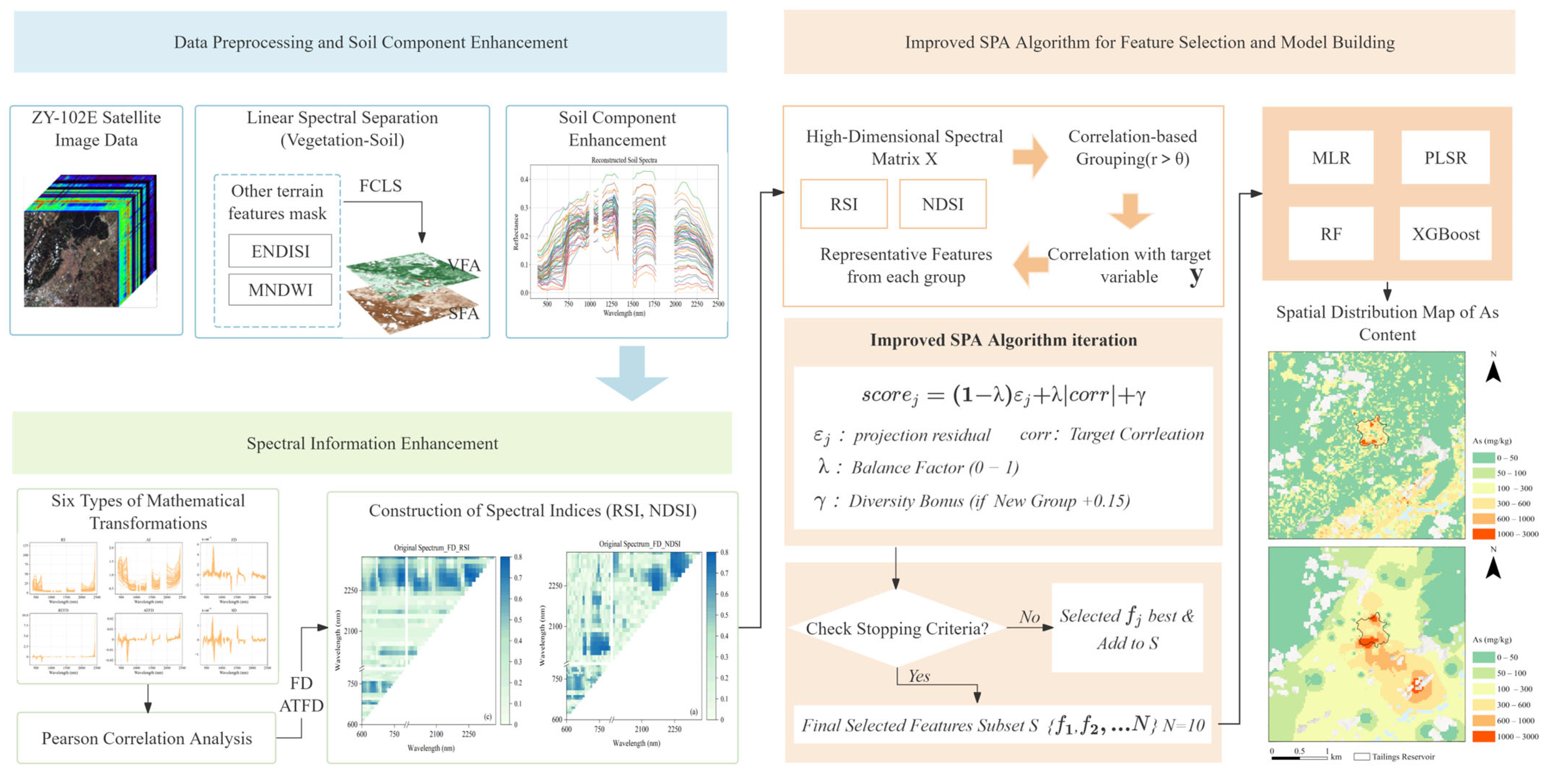
In summary, although current spaceborne hyperspectral soil heavy metal inversion studies have made some progress, limitations related to complex land cover, weak spectral responses, and limited model universality make it difficult to achieve stable, high-precision estimation in mining areas with strong vegetation interference and weak spectral characteristics. The vegetation cover in the Sanlisha’an mining area is relatively complex, particularly around the tailings reservoir area where plant species are diverse and densely concentrated. This unique vegetation cover poses challenges to extracting remote sensing signals and accurately inverting soil spectra. Therefore, the purpose of this study is to develop and validate a hyperspectral soil arsenic concentration inversion technique tailored for the complex land cover conditions of the Sanlisha’an mining area. By spectral unmixing and soil spectral enhancement, the stability and accuracy of arsenic concentration estimation at the local scale are improved. The specific workflow is as follows (Figure 1):

• Based on the ZY-1 02E satellite hyperspectral data, the FCLS linear spectral separation method was applied to enhance the soil spectral contribution, mitigating vegetation interference on soil spectral signals for subsequent As concentration inversion analysis.
• Six mathematical transformations were applied to both the original and soil component enhanced spectral data. Spectral features strongly correlated with soil As concentration were selected based on Pearson correlation coefficients. Considering the indirect spectral response characteristics between heavy metals and soil active substances, the transformed data were used to construct the Ratio Spectral Index (RSI) and Normalized Difference Spectral Index (NDSI) to enhance potential spectral information related to As concentration.
• The correlation coefficient matrix between RSI/NDSI indices and As concentration was calculated. An improved Successive Projection Algorithm (SPA) was employed to select sensitive feature band combinations for As concentration. Based on these selected bands, four As concentration estimation models—Multiple Linear Regression (MLR), Partial Least Squares Regression (PLSR), Random Forest (RF), and eXtreme Gradient Boosting (XGBoost) models were constructed for As concentration estimation. The predictive performance of models under different spectral transformation and modeling method combinations was compared to select the best inversion model.
• Finally, pixel-level spatial distribution maps of soil As concentration were generated for the study area using satellite hyperspectral imagery, and the spatial distribution characteristics of As concentration were analyzed.

2. Materials and Methods

2.1. Study Area

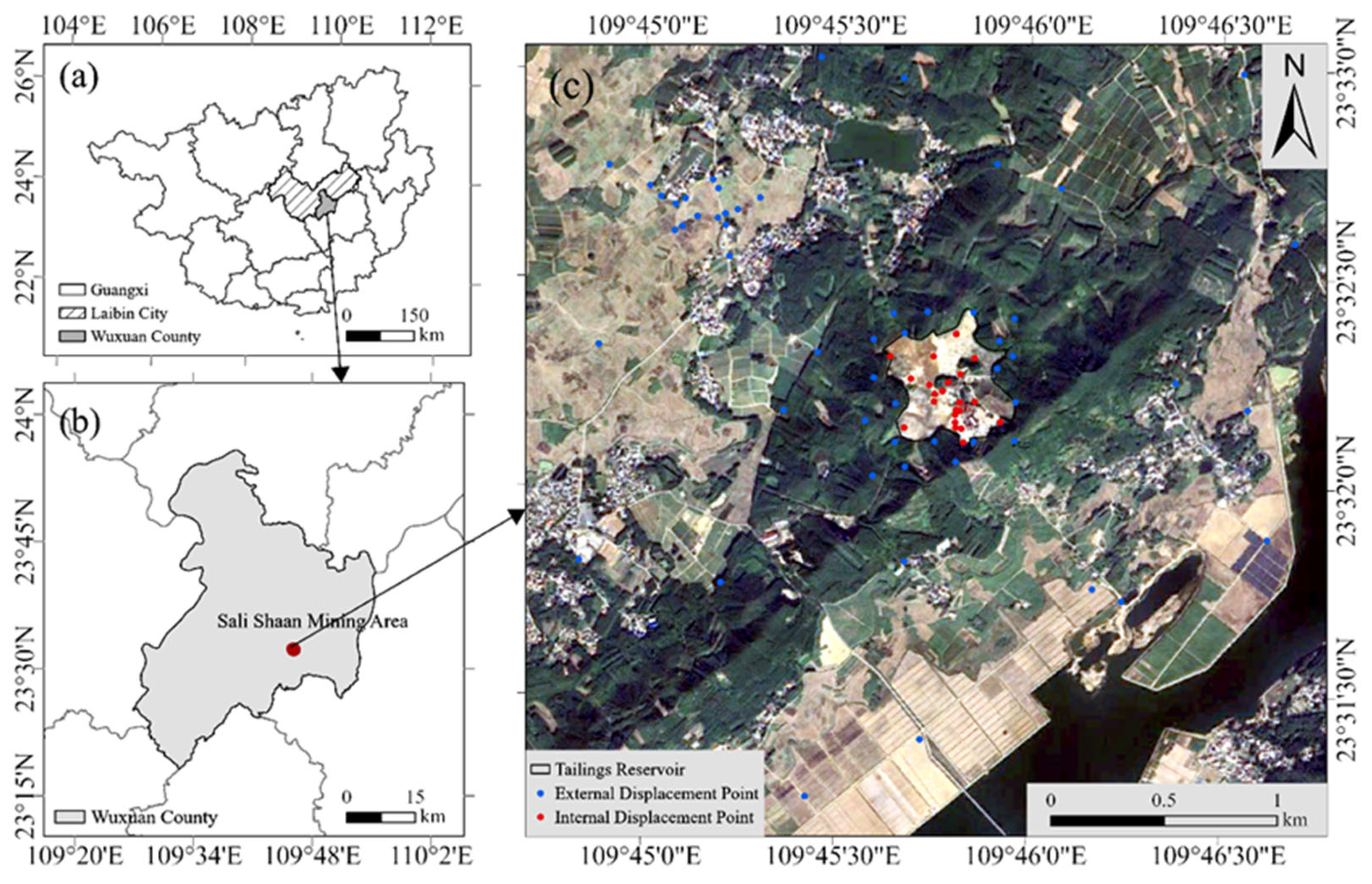
The Sanlisha’an mining area is located southeast of Sha’an Village, Sanli Town, Wuxuan County, Guangxi (109.761°E, 23.539°N). The tailings reservoir within the mining area was initially constructed in 1979. The mineral-processing plant was completed and operations commenced in 2008, with a processing capacity of 1000 t/d in the tailings reservoir, and the production ceased in 2018. Field surveys indicated substantial accumulation of solid waste within the mining area. Exposed soils showed significantly higher concentrations of heavy metals, including arsenic (As), lead (Pb), and chromium (Cr). Under the influence of rainfall leaching, these heavy metal pollutants may migrate and spread, posing potential contamination risks to surrounding groundwater, surface water, and downstream farmland. Based on field sampling, a square study area of approximately 3000 m on each side was selected, centered on the Sanlisha’an mining area (Figure 2). The feasibility of hyperspectral inversion for heavy metals was investigated using arsenic as a case study.

2.2. Monitoring Soil Arsenic Concentration in the Field

In August 2023, a field survey of soil heavy metals was conducted in the research area, and 80 valid measurement points were obtained: 22 in the mining area and 58 in the surrounding regions. Soil As concentration was measured using the five-point in situ XRF method. The equipment used was the Olympus DELTA DPO 4050 handheld XRF analyzer (Manufacturer: Olympus Scientific Solutions Americas, Waltham, MA, USA). At each measurement point, a 1 m × 1 m sample plot was marked, and in situ X-ray fluorescence measurements were taken at the four corners and the center of each plot. Before taking measurements, surface debris, including loose rocks and vegetation remnants, was removed to ensure the probe directly contacted the exposed soil surface, minimizing interference from non-soil materials. The average As concentration from the five measurement points within each plot was calculated as the representative value for that plot. This method enhances measurement efficiency while reducing the impact of micro-scale spatial heterogeneity on individual point results.

2.3. Spectral Data Acquisition and Preprocessing

2.3.1. ZY-1 02E Hyperspectral Image Preprocessing

Considering data quality and availability, the ZY-1 02E hyperspectral data (AHSI) that was acquired on 25 July 2022 was selected. This date features imaging timing close to the period of field investigation and high atmospheric transparency with no cloud cover. The data provides a spatial resolution of 30 m, with spectral resolution of 10 nm in the 387–1030 nm visible–near-infrared range (VNIR); spectral resolution of 20 nm in the 1009–2509 nm shortwave infrared region range (SWIR); and a total of 166 spectral bands. Using the ENVI 5.6 platform, the raw ZY-1 02E hyperspectral imagery was processed sequentially, including radiometric calibration, atmospheric correction, orthorectification, and Savitzky–Golay (SG) smoothing (window size = 9). Ultimately, bands affected by water vapor (1110–1144 nm, 1346–1464 nm, 1801–1953 nm, and 2458–2509 nm) were removed. Due to the overlap between the VNIR and SWIR regions, the 1005–1043 nm band was also removed. After removing these bands, the number of bands decreased from 166 to 138.

2.3.2. Soil Spectral Contribution Enhancement Based on Linear Spectral Separation

In order to address the issue of soil–vegetation mixed pixels and enhance the extraction of valid soil spectral information in areas with significant vegetation coverage surrounding mining areas, this study applies a Linear Spectral Mixing Model (LMM) combined with index-masking and end-member extraction techniques for soil spectral contribution enhancement.

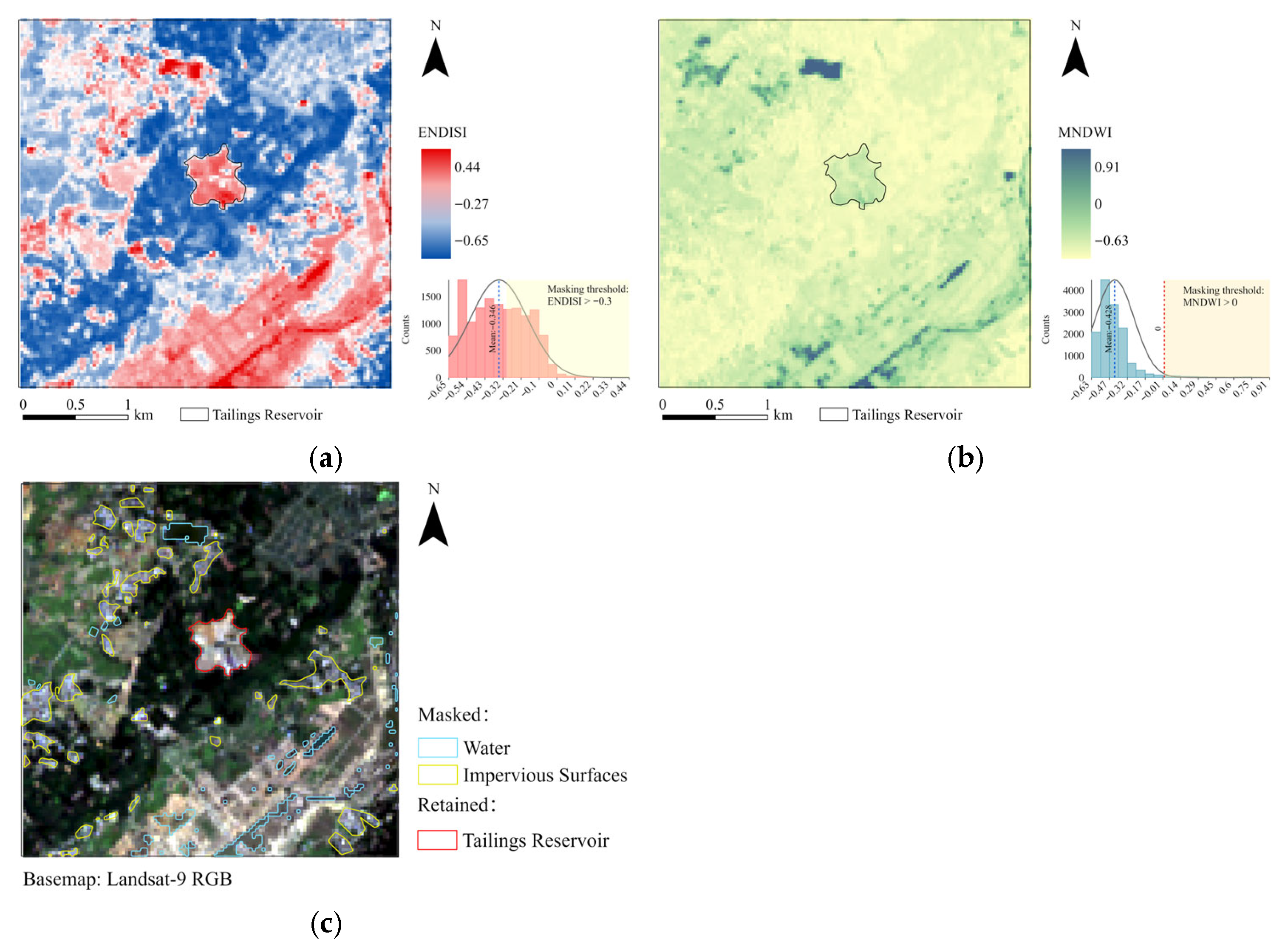
Landsat 9 multispectral imagery was selected close in time to the ZY-1 02E hyperspectral data. Enhanced Normalized Difference Impervious Surface Index (ENDISI) and Modified Normalized Difference Water Index (MNDWI) were calculated to mask impervious surfaces and bodies of water within the study area, thereby reducing interference in subsequent spectral analysis. First, the water body mask was applied, and then the impervious surface mask was applied to ensure the water body does not conflict with the impervious surface mask.

• The MNDWI calculation formula is as follows:

$$\mathit{MNDWI}= {\displaystyle \frac{{\mathit{R}}_{\mathit{g}} { \mathit{R}}_{{\mathit{SWIR}}_1}}{{\mathit{R}}_{\mathit{g}}+{ \mathit{R}}_{{\mathit{SWIR}}_1}}}$$

(1)

where ${\mathit{R}}_{\mathit{g}}$ denotes the reflectance of the green band in Landsat 9 imagery, and ${ \mathit{R}}_{{\mathit{SWIR}}_1}$ denotes the reflectance of the shortwave infrared band in Landsat 9 imagery. This study sets the threshold MNDWI > 0 to identify water bodies [45] and ≤0 for non-water bodies.

• The ENDISI calculation formula is as follows:

$$\begin{array}{c}\mathit{E}\mathit{N}\mathit{D}\mathit{I}\mathit{S}\mathit{I}={\displaystyle \frac{\left(\frac{2{\mathit{R}}_{\mathit{Blue}}+{\mathit{R}}_{{\mathit{SWIR}}_2}}{2}\right)-\left(\frac{{\mathit{R}}_{\mathit{Red}}+{\mathit{R}}_{\mathit{NIR}}+{\mathit{R}}_{{\mathit{SWIR}}_1}}{3}\right)}{\left(\frac{2{\mathit{R}}_{\mathit{Blue}}+{\mathit{R}}_{{\mathit{SWIR}}_2}}{2}\right)+\left(\frac{{\mathit{R}}_{\mathit{Red}}+{\mathit{R}}_{\mathit{NIR}}+{\mathit{R}}_{{\mathit{SWIR}}_1}}{3}\right)}}\end{array}$$

(2)

where ${\mathit{R}}_{\mathit{Blue}}$, ${\mathit{R}}_{\mathit{Red}}$, and ${\mathit{R}}_{\mathit{NIR}}$ denote the reflectance values of the blue, red, and near-infrared bands in Landsat 9 imagery, respectively. ${\mathit{R}}_{{\mathit{SWIR}}_1}$and ${\mathit{R}}_{{\mathit{SWIR}}_2}$ correspond to the reflectance values of the two shortwave infrared bands in Landsat 9 imagery.

Typically, ENDISI > 0 can be used to identify construction land [46]. However, the study area is mainly cropland, with significant changes in vegetation mixing and soil moisture, which weakens the impervious surface contrast characteristics. As a result, the ENDISI value is generally low—mostly negative. Based on high-resolution imagery and field survey data, this study identified typical construction land areas, extracted samples, and conducted statistical analysis. The results show that the ENDISI values of these regions primarily range from −0.3 to 0.2. Therefore, ENDISI > −0.3 is selected as the threshold for impervious surface classification.

The minimum noise fraction (MNF) transformation was performed on the masked imagery to highlight high signal-to-noise ratio information and reduce data dimensions, retaining components (the top 5 bands) with more than 80% of the accumulated information cotent. Then, the Pixel Purity Index (PPI) algorithm was applied for iterative calculation (number of iterations = 10,000, threshold Factor = 2.5). High-purity pixels extracted by the PPI were visually interpreted using high-resolution imagery (e.g., Google Earth, JL-1 satellite imagery). The regions entirely covered by vegetation and bare soil areas were selected, and the spectral average of the selected pixels served as the final pure vegetation and pure soil end-members.

Based on the extracted pure end-members, the FCLS method was employed to decompose mixed pixels and estimate the abundance of soil and vegetation within each pixel. FCLS adopts a linear spectral mixture model [47] and introduces non-negativity and sum-to-one abundance during the deconvolution process. Its core expression is expressed as follows:

$${\mathit{R}}_{\mathit{i}} ={\displaystyle \sum _{\mathit{k} = 1}^{\mathit{m}}}{\mathit{f}}_{\mathit{k}}{\mathit{r}}_{\mathit{ik}} + {\mathit{\epsilon }}_{\mathit{i}}\hspace{1em}{\displaystyle \sum _{\mathit{k} = 1}^{\mathit{m}}}{\mathit{f}}_{\mathit{k}}= 1, 0 < {\mathit{a}}_{\mathit{i}} < 1$$

(3)

where ${\mathit{R}}_{\mathit{i}}$ denotes the spectral reflectance of the pixel in band$i$; m represents the total number of end-members; ${\mathit{f}}_{\mathit{k}}$ is the abundance (area proportion) of end-member, $k$, within that pixel; ${\mathit{r}}_{\mathit{ik}}$is the pure spectral reflectance of the end-member, $k$, in band, $i$; and ${\mathit{\epsilon }}_{\mathit{i}}$ is the residual error term for band, i, typically comprising model error and measurement noise. This study employs iterative optimization to minimize the residual squared sum (${{\mathit{\epsilon }}_{\mathit{i}}}^2$) while approaching 0. Simultaneously, non-negative constraints are introduced to ensure the abundance estimates are physically meaningful.

After mask extraction, end-member extraction, mixed pixel unmixing, and optimization, the final spectral model can be simplified, considering only soil and vegetation conditions:

$$\begin{array}{c}{\mathit{R}}_{\mathit{i}} = \end{array}\begin{array}{c}{\mathit{f}}_{\mathit{s}}{ \mathit{r}}_{\mathit{i},\mathit{s}} + {\mathit{f}}_{\mathit{v}}{ \mathit{r}}_{\mathit{i},\mathit{v}} \end{array}$$

(4)

where${ \mathit{f}}_{\mathit{s}}$ denotes the pixel soil abundance, ${\mathit{r}}_{\mathit{i},\mathit{s}}$ represents the reflectance of soil in the i-th band, ${\mathit{f}}_{\mathit{v}}$ denotes the pixel vegetation abundance, and ${\mathit{r}}_{\mathit{i},\mathit{v}}$ represents the reflectance of vegetation in the i-th band.

Based on a simplified model, vegetation contributions were estimated using abundance results and partially compensated for within the mixed pixel reflectance. Subsequently, residual reflectance was adjusted according to soil abundance, thereby mitigating the vegetation mixing effect while enhancing the relative contribution of the soil component. The specific formula is as follows:

$${\mathit{R}}_{\mathit{soil-enhanced}} ={\displaystyle \frac{{\mathit{R}}_{\mathit{i}}-{\mathit{f}}_{\mathit{v}}{ \mathit{r}}_{\mathit{i},\mathit{v}}}{1 - {\mathit{f}}_{\mathit{v}}}}$$

(5)

where ${\mathit{R}}_{\mathit{soil-enhanced}}$ represents the soil component enhanced reflectance, with the remaining parameters as defined above.

After completing soil spectral enhancement, quality control steps are implemented to exclude unreliable samples. When the vegetation abundance exceeds 0.7, the enhanced soil spectra typically show distortion, accompanied by abnormal negative reflectance values, indicating that the soil contribution within mixed pixels is insufficient for reliable estimation. As a result, the samples with vegetation abundance > 0.7 are excluded from the subsequent analysis to ensure the reliability of the data used for modeling.

2.4. Feature Extraction and Model Construction

2.4.1. Spectral Index Construction

Spectral transformations can enhance the weak spectral responses of heavy metals in soil, emphasize characteristic information in sensitive bands, and reduce atmospheric and background noise interference, thus effectively revealing biological and chemical components relevant to the target variables [37,48]. In this study, based on ZY-1 02E hyperspectral imagery, pixel-level spectral reflectance corresponding to field sampling locations was extracted from the imagery according to the coordinates recorded during field surveys. These data underwent six mathematical transformations: reciprocal transformation (RT), reciprocal logarithmic transformation (AT), first-order derivative (FD), reciprocal first-order derivative (RTFD), reciprocal logarithmic first-order derivative (ATFD), and second-order derivative (SD). Similarly, the soil component enhanced spectral used identical transformations to enhance spectral features. The specific formulas of each transformation are given as follows:

• Reciprocal Transformation (RT)

$${\mathit{R}}_{\mathit{RT}} (\mathit{\lambda }) ={\displaystyle \frac{1}{\mathit{R}\left(\mathit{\lambda }\right)}}$$

(6)

where ${\mathit{R}}_{\mathit{RT}} (\mathit{\lambda })$ is the reciprocal transformed spectral reflectance value, and R(λ) is the spectral reflectance at the center wavelength λ.

• Reciprocal Logarithmic Transformation (AT)

$${\mathit{R}}_{\mathit{AT} }(\mathit{\lambda }) =\mathit{log} \left[{\mathit{R}}_{\mathit{RT}}\left(\mathit{\lambda }\right)\right]$$

(7)

where ${\mathit{R}}_{\mathit{RT}} (\mathit{\lambda })$ denotes the spectral reflectance after inverse logarithmic transformation, and R(λ) is defined as above.

• First-Order Derivative (FD)

$${\mathit{R}}^{\prime }({\mathit{\lambda }}_i)={\displaystyle \frac{\mathit{R} \left({\mathit{\lambda }}_{\mathit{i}+1}\right) - \mathit{R} \left({\mathit{\lambda }}_{\mathit{i}-1}\right)}{{\mathit{\lambda }}_{\mathit{i}+1}-{\mathit{\lambda }}_{\mathit{i}-1}}}$$

(8)

where ${\mathit{\lambda }}_i$ denotes the center wavelength of the i-th band (in nm), and ${\mathit{\lambda }}_{\mathit{i}-1}$ and ${\mathit{\lambda }}_{\mathit{i}+1}$ denote the center wavelengths of the preceding and succeeding bands adjacent to ${\mathit{\lambda }}_i$, respectively. $\mathit{R} \left({\mathit{\lambda }}_{\mathit{i}+1}\right)$ and $\mathit{R} \left({\mathit{\lambda }}_{\mathit{i}-1}\right)$ represent the spectral reflectance of pixels at the corresponding wavelengths.

Combining the reciprocal transform with the first-order differential yields the reciprocal first-order differential transform formula:

$${\mathit{R}}_{\mathit{RT}}^{\prime } ({\mathit{\lambda }}_i) ={\displaystyle \frac{{\mathit{R}}_{\mathit{RT} }\left({\mathit{\lambda }}_{\mathit{i}+1}\right) - {\mathit{R}}_{\mathit{RT} }\left({\mathit{\lambda }}_{\mathit{i}-1}\right) }{{\mathit{\lambda }}_{\mathit{i}+1} - {\mathit{\lambda }}_{\mathit{i}-1}}}$$

(9)

Combining the reciprocal logarithmic transform with first-order differentiation yields the reciprocal logarithmic first-order differential transform formula:

$${ \mathit{R}}_{\mathit{AT}}^{\prime } ({\mathit{\lambda }}_i)={\displaystyle \frac{{\mathit{R}}_{\mathit{AT}} ({\mathit{\lambda }}_{\mathit{i}+1}) - {\mathit{R}}_{\mathit{AT}} ({\mathit{\lambda }}_{\mathit{i}-1})}{{\mathit{\lambda }}_{\mathit{i}+1} - {\mathit{\lambda }}_{\mathit{i}-1}}}$$

(10)

• Second-Order Derivative (SD)

$${ \mathit{R}}^{″} ({\mathit{\lambda }}_i) ={\displaystyle \frac{{\mathit{R}}^{\prime }\left({\mathit{\lambda }}_{\mathit{i}+1}\right) - {\mathit{R}}^{\prime }\left({\mathit{\lambda }}_{\mathit{i}-1}\right)}{{\mathit{\lambda }}_{\mathit{i}+1} - {\mathit{\lambda }}_{\mathit{i}-1}}}={\displaystyle \frac{\mathit{R}({\mathit{\lambda }}_{\mathit{i}+1}) - 2\mathit{R}\left({\mathit{\lambda }}_{\mathit{i}}\right)+\mathit{R}({\mathit{\lambda }}_{\mathit{i}-1})}{{({\mathit{\lambda }}_{\mathit{i}+1} - {\mathit{\lambda }}_{\mathit{i}-1})}^2}}$$

(11)

where all parameters are defined as above.

To improve the accuracy of inversion for heavy metal content further, RSI and NDSI were constructed based on the transformed spectral data, and Pearson correlation analysis was conducted to evaluate their relationships with soil As concentration. The specific calculation formula is as follows:

$$\mathit{RSI} = {\displaystyle \frac{\mathit{R}\left({\mathit{\lambda }}_{\mathit{i}}\right)}{\mathit{R}\left({\mathit{\lambda }}_{\mathit{j}}\right)}}$$

(12)

$$\mathit{NDSI}={\displaystyle \frac{\mathit{R}({\mathit{\lambda }}_{\mathit{i}}) - \mathit{R}({\mathit{\lambda }}_{\mathit{j}})}{\mathit{R}\left({\mathit{\lambda }}_{\mathit{i}}\right)+\mathit{R}\left({\mathit{\lambda }}_{\mathit{j}}\right)}}$$

(13)

where $\mathit{R}\left({\mathit{\lambda }}_{\mathit{i}}\right)$ denotes the spectral reflectance at the center wavelength of the i-th band (in nm), and $\mathit{R}\left({\mathit{\lambda }}_{\mathit{j}}\right)$ refers to the spectral reflectance at the center wavelength of the j-th band.

2.4.2. Feature Selection Using an Improved Successive Projection Algorithm (SPA)

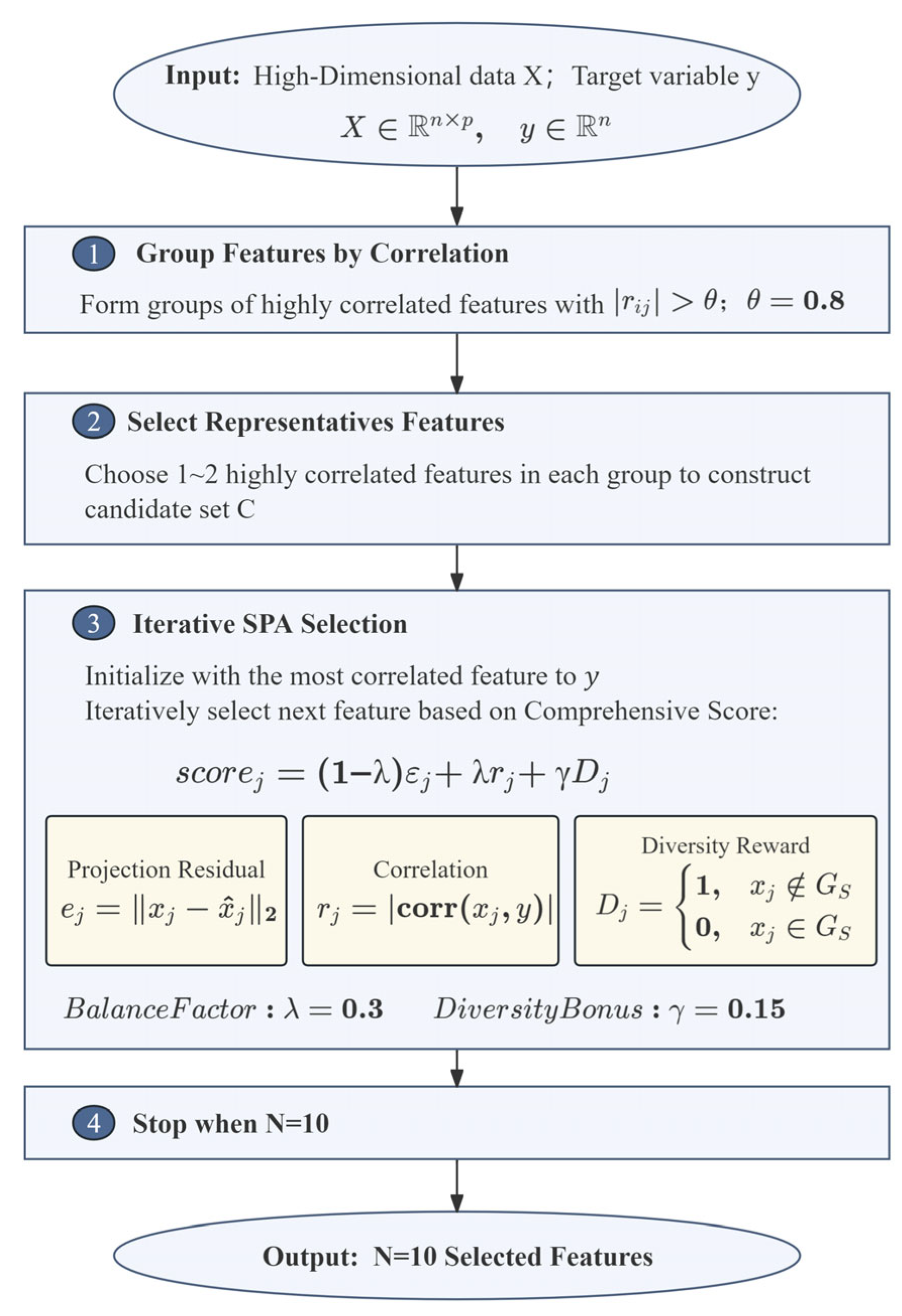
In order to improve model predictive performance, this study employed the Successive Projection Algorithm (SPA) to select features in high-dimensional spectral data. This study further improves this approach by integrating feature correlation, diversity, and projection residual constraints (Figure 3). First, features are grouped based on their pearson correlation coefficients. When |r_ij| > 0.8, the features are considered highly correlated and assigned to the same group to identify potential collinearity structures. Subsequently, the feature with the highest correlation to the target variable, y, is selected as the representative feature within each group to form the candidate feature set, C.

Iterative selection is performed on the candidate set, C: the feature most correlated with the target variable is selected as the initial feature. For each unselected feature, the following was calculated: its projection residual, e_j, on the selected subset; its correlation, r_j, with the target variable; and its diversity contribution, Dj, from the new feature group. The composite scoring function is defined as

$${\mathit{score}}_{\mathit{j}}=(1 - \mathit{\lambda }) {\mathit{e}}_{\mathit{j}}+\mathit{\lambda }{\mathit{r}}_{\mathit{j} }+\mathit{\gamma }{\mathit{D}}_{\mathit{j}}$$

(14)

where λ = 0.3 balances independent information with target relevance, and γ = 0.15 represents the diversity reward weight to encourage cross-group selection and reduce redundancy. In each iteration, the feature with the highest composite score is added to the feature subset.

Feature selection terminates when N = 10 is reached. This threshold is determined under the conditions of small-sample high-dimensional data (n = 56). Approximately $\sqrt{\mathit{n}}~\mathit{n}/5$ variables are selected to preserve sufficient spectral information while avoiding overfitting.

2.4.3. As Concentration Inversion Model Construction

Four models—traditional regression models (MLR and PLSR) and ensemble learning models (RF and XGBoost)—were used for soil As content inversion analysis. As a baseline regression method, MLR establishes a clear linear relationship between feature and target variables through least squares estimation, which is characterized by simple structure and high interpretability. PLSR combines principal component analysis with Multiple Linear Regression to achieve feature dimension reduction and predictive modeling. Its core parameter (optimal number of latent variables) was determined through 5-fold cross-validation within the range of 1 to n (where n is the number of input feature bands). As an ensemble learning algorithm, RF builds multiple decision trees and aggregates their predictions, effectively reducing overfitting risk and enhancing model generalization capability. XGBoost significantly improves modeling accuracy and computational efficiency by integrating parallel computing and efficient iteration mechanisms with traditional gradient boosting decision tree (GBDT). Both RF and XGBoost hyperparameters were iteratively adjusted using grid search combined with 5-fold cross-validation, with cross-validated R² serving as the primary model selection metric. Specific search ranges are detailed in

Table 1. Hyperparameter search ranges of RF and XGBoost models.

Random Forest		XGBoost
Hyperparameter	Search Range	Hyperparameter	Search Range
n_estimators	[50, 200]	n_estimators	[50, 200]
max_depth	[2, 5]	max_depth	[2, 5]
min_samples_split	[2, 10]	learning_rate	[0.05, 0.2]
min_samples_leaf	[2, 10]	subsample	[0.5, 1]
max_features	[0.2, 0.8]	colsample_bytree	[0.5, 1]
		reg_alpha	[0, 1]
		reg_lambda	[0, 1]

.

In order to ensure comparability among models, all four models used repeated random sub-sampling validation for final performance evaluation, repeated 10 times. For each validation iteration, the dataset was split with a fixed test set proportion of 0.3, using different random seeds (random seed = 42 + 100 × i, i = 1…10). The performance of the final model was evaluated using the average of R² and RMSE across all 10 iterations as the composite metric.

2.4.4. Accuracy Evaluation

The model’s predictive accuracy is assessed using two metrics: the coefficient of determination (R²) and the root mean square error (RMSE). R², also known as the coefficient of determination, which ranges from 0 to 1. Values closer to 1 indicate better model fit and greater stability. RMSE measures the deviation between model predictions and actual observations; smaller values signify predictions closer to true values. R² and RMSE can be used to comprehensively compare the predictive performance of different models.

3. Results

3.1. Statistical Analysis of As Concentration

Since spectral signals in areas with high vegetation cover are typically affected by the mixed pixel effects, samples with vegetation abundance exceeding 0.7 were removed. Ultimately, 56 samples containing sufficient soil information were retained for subsequent analysis (including 22 tailings reservoir samples and 34 samples from the surrounding area of the tailings reservoir).

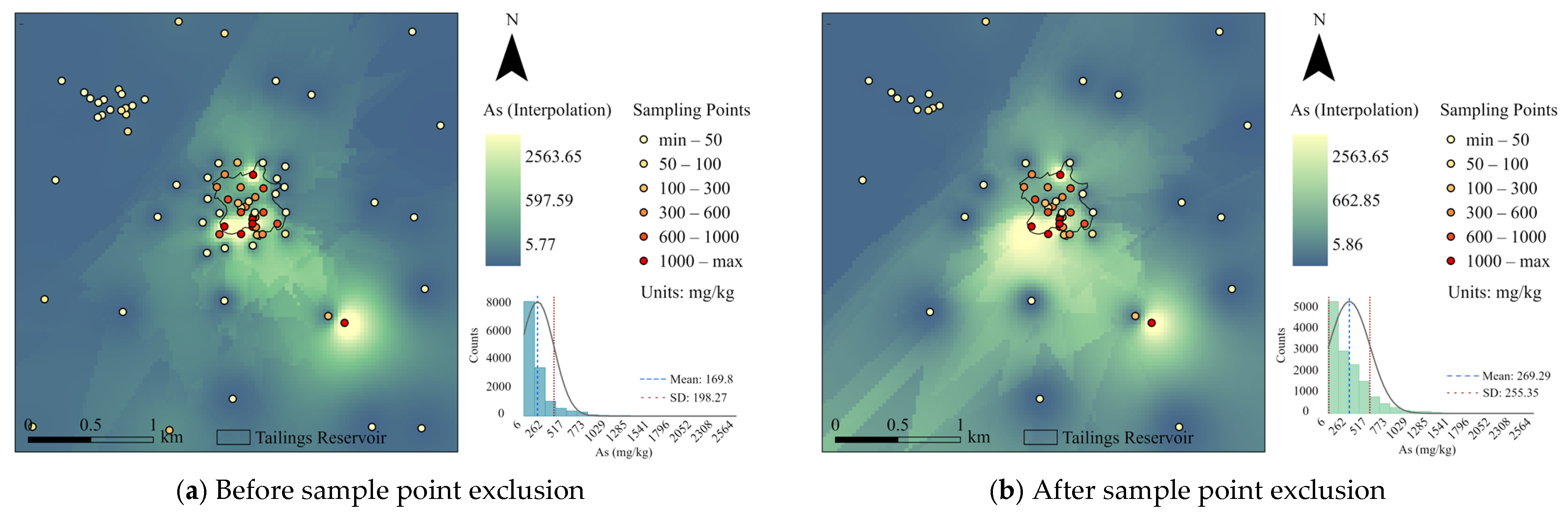
The As concentration of the sampling points before and after exclusion were classified into concentration levels, and the spatial interpolation was used for comparison (Figure 4). After sample exclusion, low-value points in the peripheral areas decreased, and the remaining samples became more concentrated in the central region. The interpolation results of the two datasets exhibited consistent high-value centers and similar diffusion directions, suggesting that the principal spatial pattern of contamination was largely preserved. Therefore, the retained samples are still representative of pollution source identification and spatial heterogeneity assessment. The statistical analysis showed that the mean As concentration increased from 169.8 mg/kg to 269.29 mg/kg, and the standard deviation increased from 198.27 mg/kg to 255.35 mg/kg, indicating higher overall concentration levels and dispersion. Meanwhile, the constraint from low-value background areas weakened, which may increase uncertainty in estimating background concentrations and regional mean levels.

The basic characteristics of As concentration in the remaining soil samples of the study area were statistically analyzed. As concentration in the samples ranged from 5.75 to 3487.56 mg/kg, with a standard deviation of 705.53 mg/kg. According to the provisions of the Soil Environmental Quality Risk Control Standard for Soil Contamination of Agricultural Land (GB15618-2018) [49] and the Soil Environmental Quality Risk Control Standard for Soil Contamination of Development Land (GB36600-2018) [50]: For industrial land within urban construction land, the risk screening value for As is 60 mg/kg, and the control value is 140 mg/kg. Most sampling points in the study area exceeded both the risk screening and control values for agricultural and industrial land. Therefore, conducting an inversion analysis of As concentration in the mining area can effectively assess pollution risks and provide scientific basis for environmental remediation.

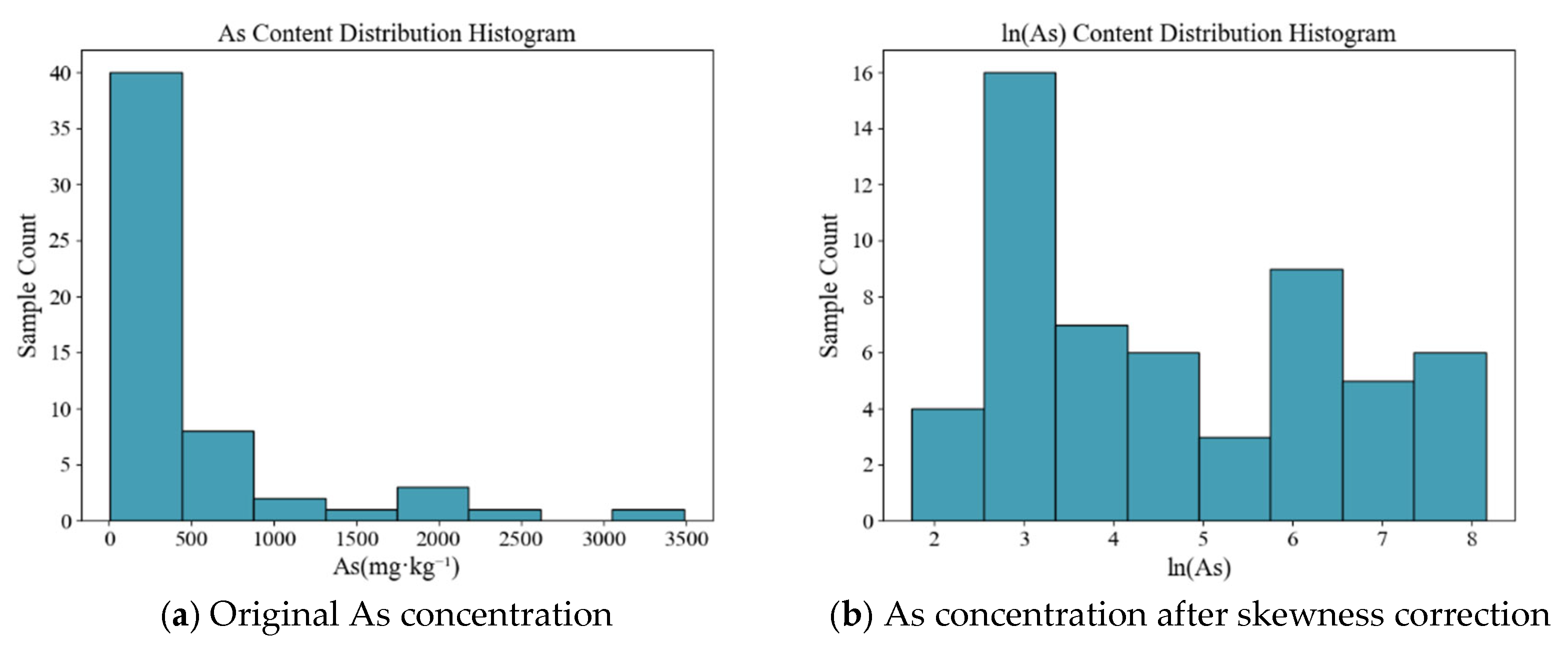
The distribution histogram of As concentrations across 56 sampling points is shown in Figure 5a. Given the severe skewness in As concentrations within the mining area, log transformation can convert severely skewed variables into approximately normally distributed ones [51]. Consequently, this study performed skewness correction on 56 sample points using natural logarithm transformation, making the distribution more balanced and reducing skewness (Figure 5b).

3.2. Soil Spectral Contribution Enhancement Results

The spatial distribution of the ENDISI and MNDWI indices for the Sanlisha’an mining area is shown in Figure 6a,b, respectively, with the masking extent depicted in Figure 6c. Thresholds were set for these two indices to mask impervious surfaces and water bodies; the thresholding process is detailed in Materials and Methods, Section 2.3.2. Although ENDISI values within the tailings reservoir exhibit typical impervious surface characteristics—primarily due to tailings deposits typically possessing high compaction and relatively flat surfaces, rendering them spectrally reflective akin to impervious surfaces and thus producing strong spectral reflectance signals—field investigations revealed that the tailings reservoir consists predominantly of bare soil. Furthermore, most sampling points were situated within the tailings reservoir itself. As a result, the tailings reservoir area was not masked, whereas impervious surfaces in surrounding residential areas were masked. However, field investigations revealed that the tailings reservoir is predominantly composed of bare soil, with most sampling points located within these ponds. Consequently, no masking was applied to the tailings reservoir areas. Instead, hardened impervious surfaces in surrounding residential areas were masked to minimize external interference and ensure the accuracy of the study results.

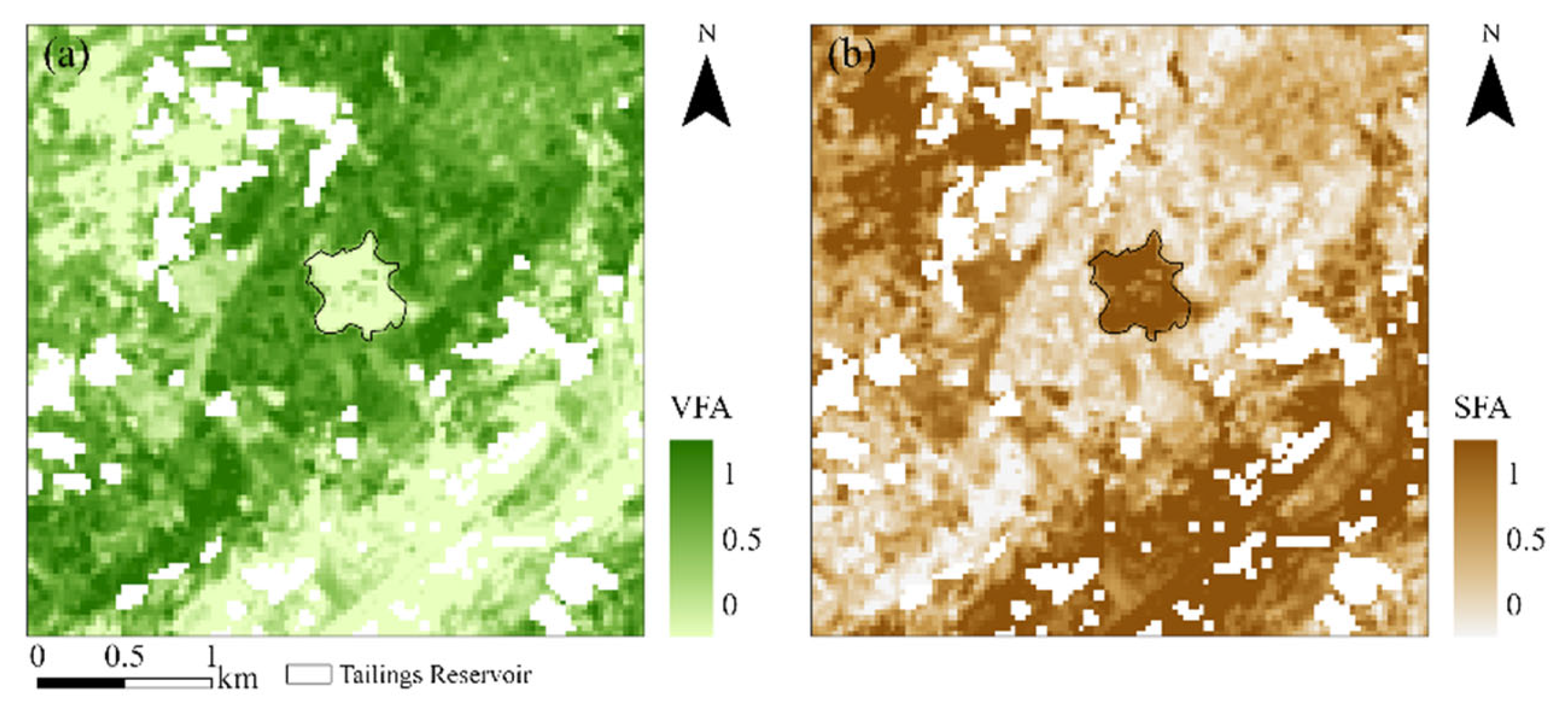
Based on the masked imagery, the ZY-1 02E images perform mixed pixel unmixing using the FCLS method, ultimately yielding spatial distribution maps of vegetation fractional abundance (VFA) and soil fractional abundance (SFA) within the study area (Figure 7a,b). As shown in these figures, soil is concentrated within the tailings reservoir with no vegetation cover, while the surrounding areas exhibit a certain degree of vegetation cover.

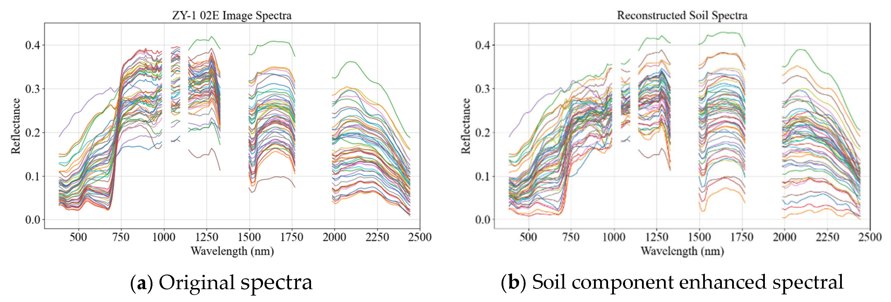
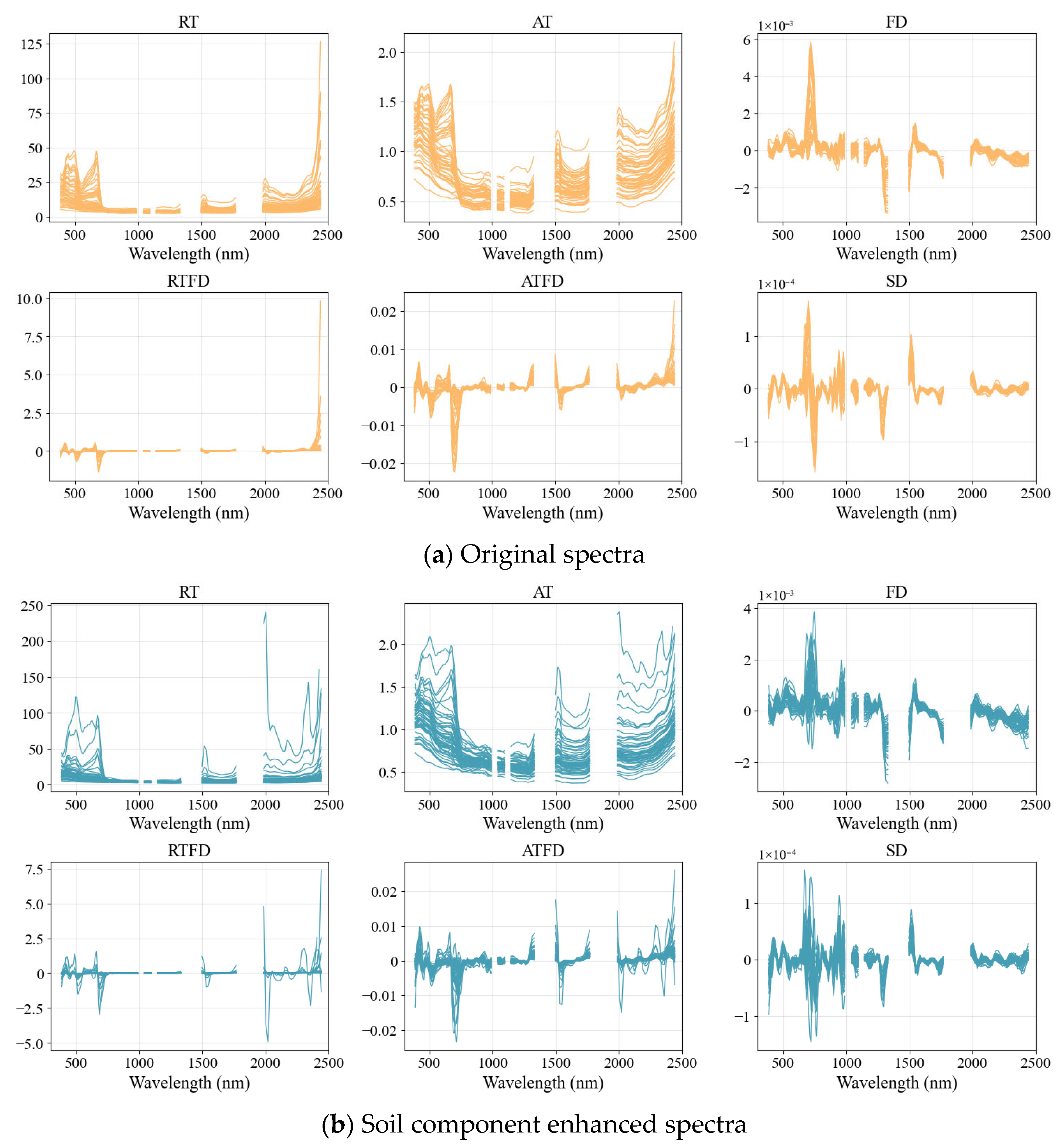
In the VNIR (visible–near-infrared) band, the original spectra exhibit significant inter-sample variation, primarily reflecting the superimposed effects of mixed vegetation and soil responses. This is most pronounced at the green reflectance peak around 550 nm. Following soil component enhancement processing, the spectral curve exhibits overall smoothing with markedly reduced near-infrared reflectance. This indicates a mitigation of vegetation-dominated strong scattering effects, alongside an enhanced contribution from soil within the overall reflectance signal.

Within the SWIR (2000–2500 nm) band, key absorption features were largely preserved, indicating that the enhancement processing did not compromise crucial spectral information related to soil physicochemical properties (Figure 8). Previous studies have identified characteristic absorption features in cellulose and lignin within dry vegetation near 2100 nm and 2300 nm [52]; simultaneously, layered silicate minerals, containing hydroxyl groups (OH) in their crystal structures, typically exhibit distinct diagnostic absorption features near 2210 nm (kaolinite, muscovite, montmorillonite, and illite) and 2340 nm (serpentine, chlorite, and talc). Some minerals also display minor absorption peaks near 2250 nm and 2380 nm [53]. Consequently, absorption characteristics in this spectral band may result from the combined effects of residual vegetation and mineral absorption. Further observation of the figure reveals that absorption structures near 2210 nm and 2340 nm are more pronounced in certain samples, indicating that the enhancement processing has, to some extent, amplified the expression of diagnostic absorptions associated with hydroxyl-bearing layered silicate minerals.

Nevertheless, faint vegetation signal features remain observable in the enhanced spectra, which is potentially attributable to multiple factors: complex sub-pixel structures at 30 m spatial resolution; inherent variability within the end-member spectra themselves; and nonlinear mixing effects arising from multiple photon scattering between the surface and vegetation. Collectively, these factors constrain the linear model’s capacity for complete separation of vegetation signals.

3.3. Spectral Transformation and Spectral Index Construction

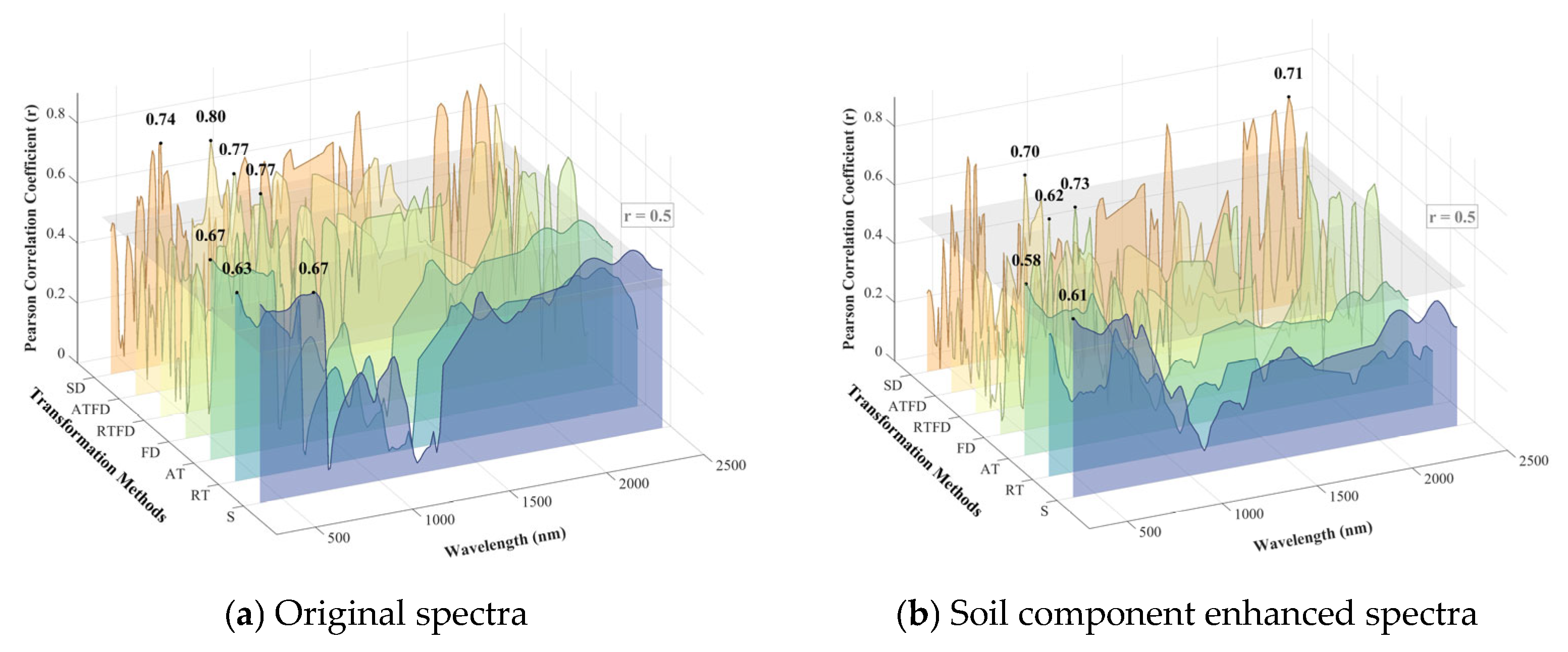
Based on the original spectral data and the soil component enhanced spectral data, six transformations—RT, AT, FD, RTFD, ATFD, and SD—were applied to eliminate interference from partial baseline and other background sources. The transformed spectra are shown in Figure 9. The correlations between soil As concentration and the original spectra (S), as well as the six transformations, were calculated for both the original and enhanced spectra (Figure 10). For the original spectra, the correlation between spectral features and soil As concentration, using six transformation methods, generally improved the correlation coefficients between spectra and soil As concentration. Among them, FD, ATFD, and RTFD performed best, yielding maximum correlation coefficients of 0.77, 0.80, and 0.77, respectively. Compared with the original spectra, the soil component enhanced spectra showed broadly consistent correlation trends. FD, ATFD, and SD performed best, with maximum correlation coefficients of 0.73, 0.71, and 0.7, respectively. Although the correlation coefficients showed slight decreases, this may be attributed to information loss during enhancement, particularly the removal of vegetation interference from the original spectra, which affected the correlation. Nevertheless, the enhanced spectra demonstrated the advantage of effective noise reduction and enhanced spectral stability, enabling more precise reflection of soil characteristics.

Studies indicate that soil organic matter, soil iron and manganese oxide, and clay minerals are key active soil components for the fixation and adsorption of heavy metals. These components show diagnostic absorption features within a specific spectral range. For instance, the presence of organic matter and its associated functional groups (e.g., hydroxyl and carboxyl groups) have a significant impact on spectral signals in the VNIR (600–800 nm) [54]. The absorption characteristics of these groups are closely related to the composition and content of humic substances, while clay minerals exhibit strong characteristic absorption troughs at wavelengths near 1900 and 2200 nm in the SWIR due to their hydroxyl and water molecule content [22]. Given the intrinsic relationship between soil active substances and soil heavy metals, two transformation methods with relatively good performance were adopted: FD and ATFD. The NDSI and RSI spectral indices were constructed using the highly correlated 600–800 nm organic matter-related spectral band and the 2000–2300 nm clay mineral-related spectral band. This approach enhances the expressiveness of key spectral features of soil active substances by expanding the spectral characteristics of soil.

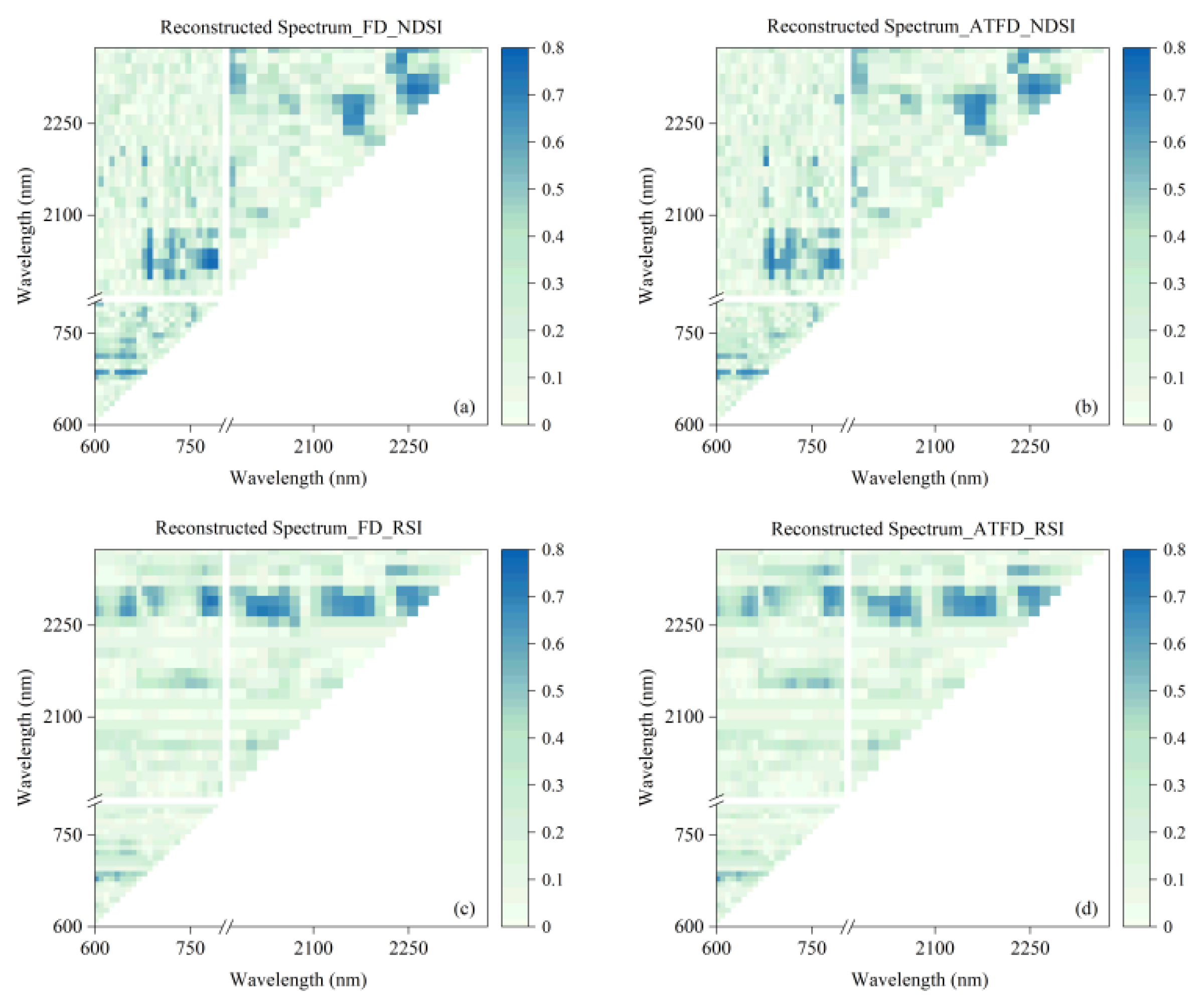
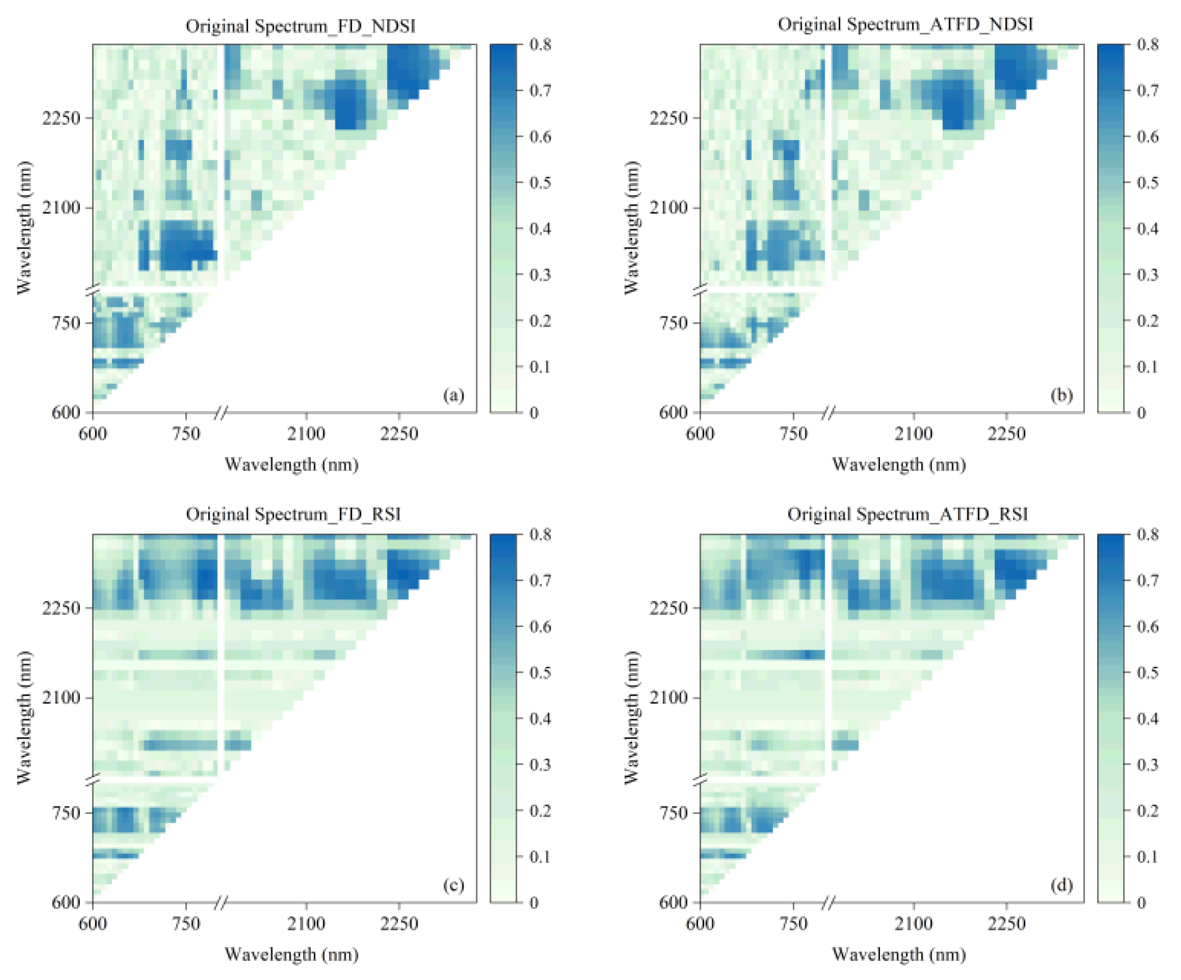
Figure 11 presents the correlation distribution between As concentration and NDSI/RSI indices derived from six original spectral transformation datasets. In Figure 11, the horizontal and vertical axes represent spectral wavelength combinations. The color gradient (from light green to dark blue) reflects the absolute values of the Pearson correlation coefficient between spectral indices and As concentration, with blue regions indicating strong correlations. The results show that the strong correlation regions (dark blue areas) for RSI and NDSI with As concentration exhibit distinct distribution patterns across wavelength combinations. For the NDSI (Figure 11a,b): its strong correlation zones predominantly appear as “point-like” or “block-like” patterns, concentrated in specific band combinations. For example, the index is more sensitive to capturing reflectance variations between two specific bands in the SWIR. For the RSI (Figure 11c,d): “striped” patterns are clearly visible in the strongly correlated regions. It is noteworthy that spectral bands within the 2100–2300 nm range exhibit a significant correlation with arsenic concentrations, suggesting that this wavelength range may serve as a key indicator band for assessing arsenic concentrations in the study area.

As can be seen in Figure 12, there is a clear correlation between the As concentration and the NDSI, as well as the RSI indices obtained through six soil enhanced spectral transformations. Compared with the correlation distribution of the original spectral indices, the correlation patterns between the enhanced spectra’s NDSI, RSI, and As concentration are largely consistent in terms of their overall trends. However, visually highly correlated areas show obvious contraction. The essence of soil component enhancement is to mitigate the interference of vegetation noise, which often leads to weak or spurious correlations in many spectral band combinations. This suggests that the enhanced spectra allow the model to more accurately and directly reflect the true physical relationship between soil composition and As concentration.

3.4. Feature Selection and Model Construction

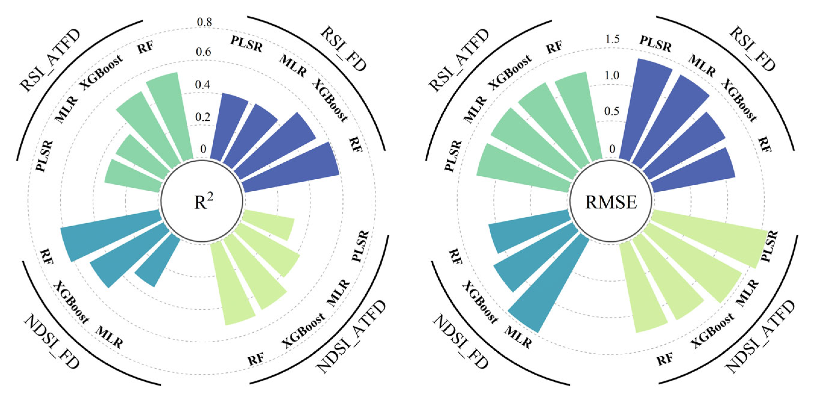
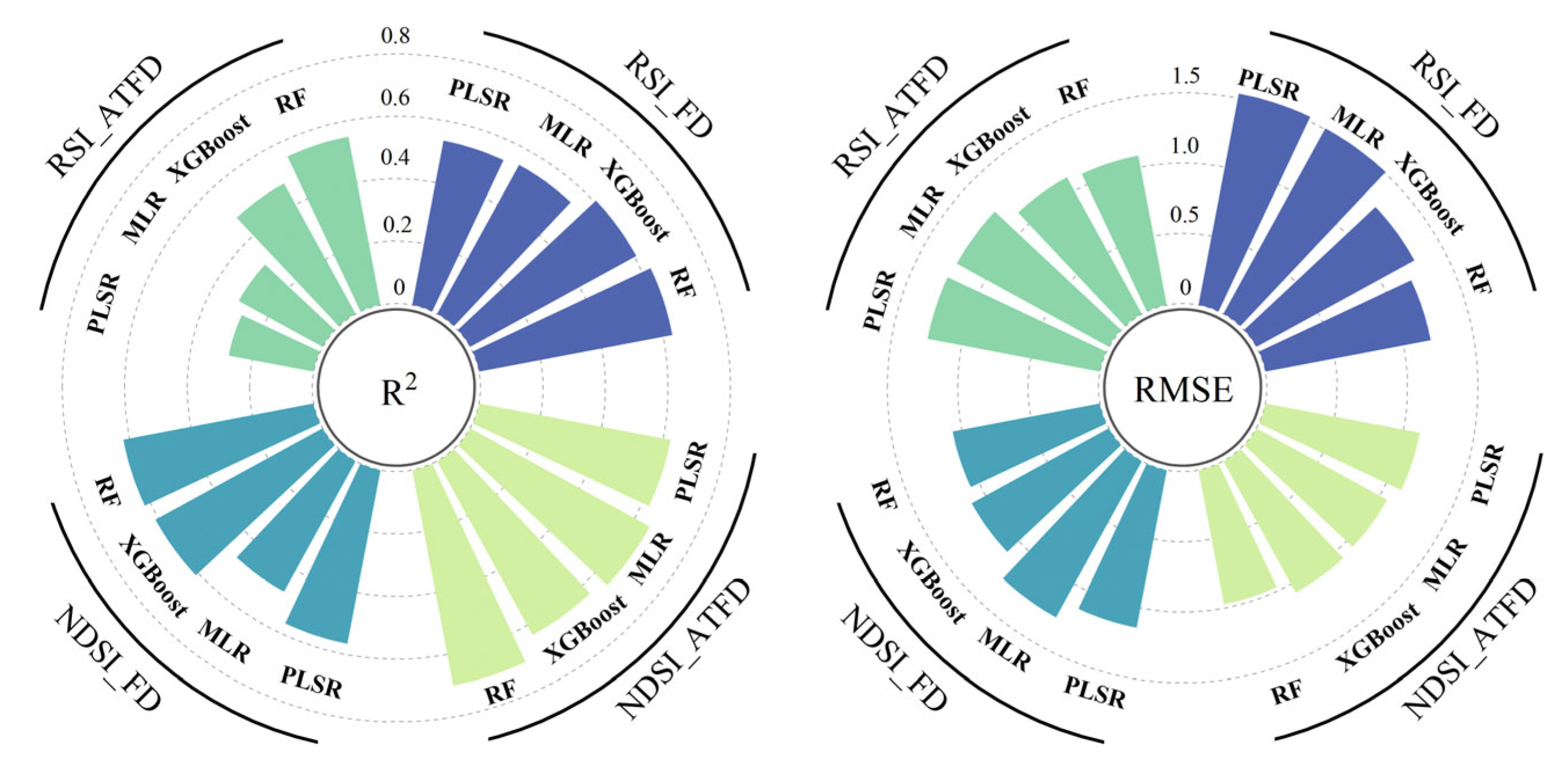
Four algorithms—MLR, PLSR, RF, and XGBoost—were employed to construct As concentration inversion models. Model performance comparisons are shown in Figure 13 and Figure 14. The detailed validation results presented in

Table 2. Modeling results for As concentration inversion of the original spectra.

Spectral Index	Transformation Method	Model	Training Set		Test Set		Feature Sequence
			R2	RMSE	R2	RMSE
NDSI	FD	MLR	0.849	0.705	0.338	1.465	R781_R2020; R618_R2121; R610_R2138; R695_R2323; R653_R2020; R2037_R2155; R2003_R2104; R601_R2172; R670_R2273; R790_R2323
		PLSR	0.864	0.667	—	—
		RF	0.823	0.764	0.617	1.103
		XGBoost	0.961	0.358	0.518	1.234
	ATFD	MLR	0.886	0.598	0.422	1.451	R2273_R2306; R2071_R2155; R781_R2256; R1986_R2087; R2121_R2205; R618_R773; R2037_R2188; R2138_R2205; R601_R2340; R635_R2104
		PLSR	0.864	0.654	0.311	1.584
		RF	0.911	0.542	0.511	1.240
		XGBoost	0.997	0.106	0.497	1.268
RSI	FD	MLR	0.762	0.880	0.417	1.379	R781_R2306; R2222_R2306; R747_R1986; R653_R2054; R670_R2205; R644_R653; R2054_R2205; R635_R2003; R773_R790; R618_R627
		PLSR	0.760	0.884	0.409	1.392
		RF	0.799	0.813	0.592	1.135
		XGBoost	0.954	0.390	0.534	1.193
	ATFD	MLR	0.752	0.950	0.336	1.278	R2256_R2306; R704_R2121; R1969_R2188; R773_R790; R678_R704; R695_R2071; R713_R798; R644_R670; R798_R2138; R747_R2087
		PLSR	0.751	0.952	0.341	1.270
		RF	0.787	0.837	0.540	1.206
		XGBoost	0.840	0.725	0.503	1.258

Notes: “—“ indicates R² values below zero; the background color represents the best-performing model in each category.

(raw spectra) and

Table 3. Modeling results for As concentration inversion of soil componentenhanced spectra.

Spectral Index	Transformation Method	Model	Training Set		Test Set		Feature Sequence
			R2	RMSE	R2	RMSE
NDSI	FD	MLR	0.790	0.835	0.477	1.268	R781_R2020; R2188_R2340; R661_R2087; R730_R2374; R2104_R2340; R2087_R2121; R781_R2087; R730_R781R781_R2222; R773_R1986
		PLSR	0.793	0.831	0.565	1.141
		RF	0.919	0.515	0.620	1.064
		XGBoost	0.938	0.451	0.610	1.111
	ATFD	MLR	0.862	0.668	0.656	1.059	R2256_R2306; R618_R773; R2003_R2256; R2087_R2222; R764_R2172; R781_R2155; R627_R2273; R670_R2323; R773_R2054; R670_R2172
		PLSR	0.866	0.656	0.623	1.117
		RF	0.910	0.544	0.701	0.971
		XGBoost	0.868	0.659	0.635	1.068
RSI	FD	MLR	0.731	0.929	0.545	1.233	R781_R2290; R1969_R2155; R747_R2256; R2087_R2104; R2104_R2138; R2020_R2306; R661_R2087; R670_R2188; R635_R653; R610_R773
		PLSR	0.729	0.933	0.536	1.247
		RF	0.909	0.547	0.629	1.082
		XGBoost	0.997	0.091	0.606	1.110
	ATFD	MLR	0.698	0.992	0.306	1.507	R2172_R2290; R2071_R2239; R773_R1986; R1986_R2155; R747_R2121; R627_R2138; R721_R790; R764_R2138; R713_R798; R695_R704
		PLSR	0.682	1.017	0.277	1.533
		RF	0.892	0.598	0.549	1.196
		XGBoost	0.941	0.440	0.477	1.281

Notes: the background color represents the best-performing model in each category.

(soil component enhances spectra). The spectral index combinations ultimately input into the model after SPA feature selection are denoted as “feature sequence” in Table 2 and Table 3. Each element in this sequence corresponds to a weight variable in the model’s regression coefficients, collectively forming the mapping relationship that converts spectral reflectance into estimated arsenic concentration values.

For the original spectra, Figure 13 and Table 2 reveal a significant difference in predictive capability among the four models. MLR and PLSR models exhibited generally low R² values on the test set, with PLSR even yielding a negative R² value. This indicates that the severe overfitting in these linear regression models prevents the effective generalization to new samples and severely limits their ability to quantitatively predict As concentration in this region. In contrast, ensemble learning algorithms performed excellently, demonstrating high R² values and low RMSE. The best model was the FD-NDSI-RF combination, which realized the training set, R², of 0.832 and a test set, R², of 0.617. This indicates that RF effectively captures the complex nonlinear relationship between soil spectral indices and As concentration.

In the analysis of enhanced spectra (Figure 14 and Table 3), ensemble learning algorithms, RF and XGBoost, also significantly outperformed traditional linear models. The best model was the ATFD-NDSI-RF combination, achieving an R² of 0.911 on the training set and 0.7 on the test set. This further demonstrates that spectral enhancement not only alters the best feature combination but also enhances the accuracy and reliability of model predictions, significantly improving the generalization capability of the model.

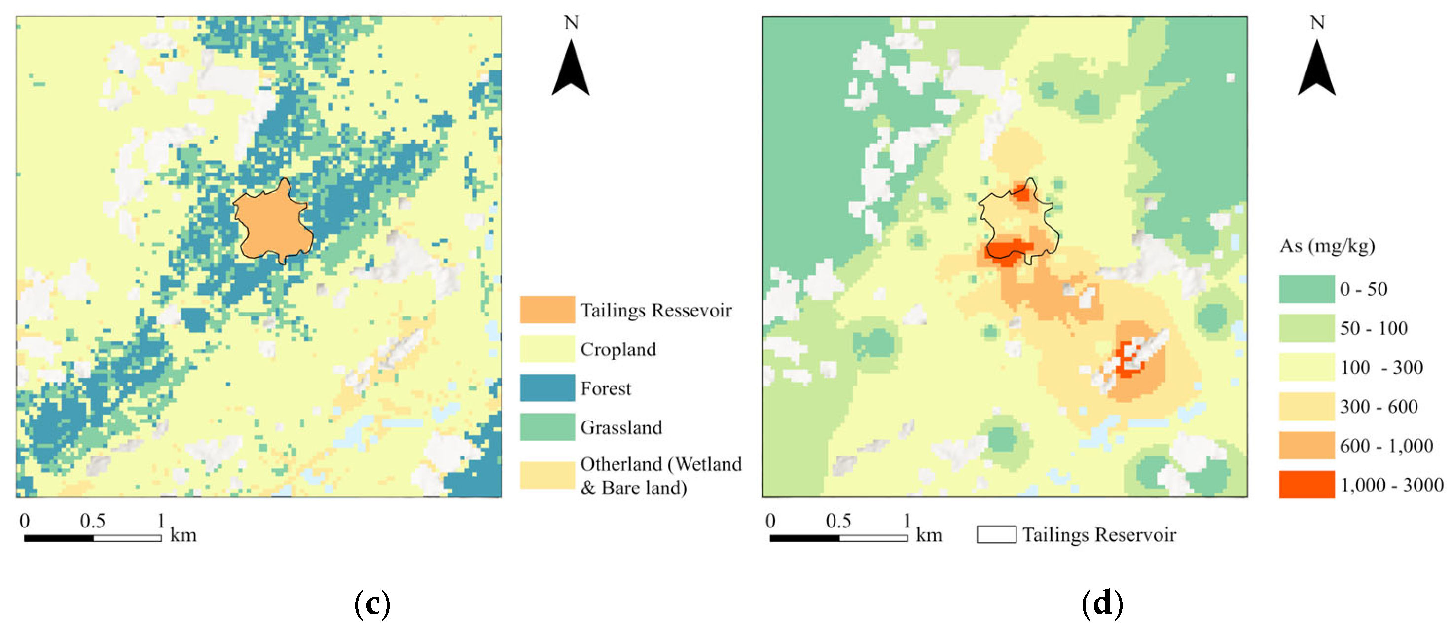
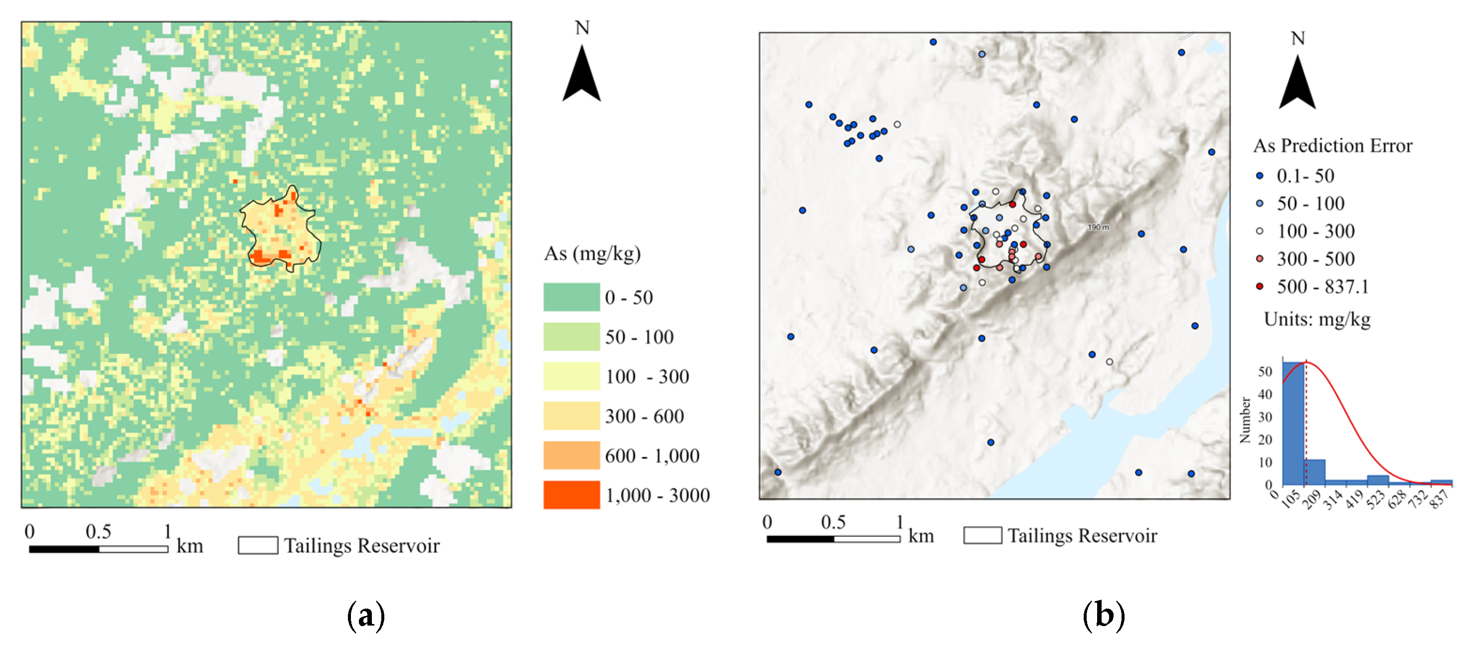
This study employed the best model combination, NDSI–ATFD–RF, to perform inversion across the entire study area, yielding a spatial distribution map of soil As concentration (Figure 15a). In order to quantitatively evaluate the spatial reliability of the inversion results, all field sampling points were used to analyze the errors between predicted and measured arsenic concentrations, as well as the spatial error distribution and zoning statistics (Figure 15b). Special attention should be paid to the fact that samples with high vegetation coverage were excluded only during the modeling phase, but retained in the spatial accuracy assessment to evaluate the applicability of the inversion results across different subregions.

Based on the 2022 GLC_FCS30 land cover dataset (spatial resolution 30 m) [55], the study area was classified into tailings reservoir, forest land, grassland, cropland, and otherland (including wetlands and bare land) (Figure 15c). The boundary of the tailings reservoir was determined through field surveys combined with visual interpretation of high-resolution imagery. Due to insufficient sample size, grassland and otherland were excluded from the statistical analysis. Figure 15b shows the spatial distribution of prediction errors, revealing that high error values are concentrated primarily in the tailings reservoir and its adjacent transition zones, whereas peripheral natural surface areas exhibit lower overall errors. This indicates that the errors exhibit distinct spatial clustering rather than a random distribution. When this is combined with the sub-area classification (Figure 15b), it can be seen that the zones highly overlap with the tailings reservoir and its surrounding impact areas. This suggests that model errors correlate with pollution intensity gradients, with greater deviations occurring in regions where concentrations are high and changing rapidly. The zoned statistical results further reveal significant spatial differences (

Table 4. Statistical results of the accuracy of As inversion in different soil zones.

Subregions	MAE	RMSE	R2	Pearson’s r
	(mg/kg)	(mg/kg)	—	—
Tailings Reservoir	257.15	342.19	0.85	0.92 ***
Forest	47.95	49.64	0.92	0.96 ***
Cropland	56.26	203.25	0.68	0.83 ***

Notes: “***” indicates p-value < 0.001.

). Although the tailings reservoir area exhibited the highest mean absolute error (MAE = 257.15 mg/kg) and root mean square error (RMSE = 342.19 mg/kg), it still showed a high correlation (correlation coefficient r = 0.92, coefficient of determination R² = 0.85). This suggests that, while the model effectively captured spatial trends in this region, it underestimated specific values. Forest areas exhibited optimal predictive performance (R² = 0.92, RMSE = 49.64 mg/kg), indicating more reliable back-calculation results in regions with relatively stable backgrounds and gradual concentration variations. Despite the relatively high root mean square error (RMSE) for the cultivated area (203.25 mg/kg), the correlation remains robust (r = 0.83). This indicates that while the model retains the overall trend, it exhibits significant numerical error. This may be due to the extensive coverage of cultivated land and pronounced surface variations, as well as the relatively dispersed sampling points, which lead to amplified local variability and errors. Overall, there are systematic error variations across subregions: areas with high concentrations and steep slopes exhibit higher errors and stronger correlations, while low-concentration background zones show lower errors and weaker correlations. This pattern demonstrates the model’s capacity to capture spatial structure; however, its representation of extreme values remains inadequate.

Furthermore, a comparison of the results of IDW interpolation reveals a similar spatial distributions to that of the other method, with higher concentrations concentrated in the tailings reservoir and in the southeastern part of the study area. However, given IDW’s sensitivity to sampling density and distance weighting, smoothing errors may occur in sparsely sampled regions. However, the sampling points within the tailings reservoir are relatively dense, which makes the interpolation results more reliable; a Pearson correlation analysis was therefore further conducted for the tailings reservoir area, yielding a correlation coefficient of 0.60. This indicates that the inversion results effectively reproduce the spatial variation trends and pollution patterns in highly contaminated areas.

4. Discussion

4.1. Evaluation of FCLS-Based Spectral Enhancement for Vegetation Interference Mitigation

In areas with high vegetation coverage, such as mining sites, spectral mixing significantly constrains the accuracy of satellite hyperspectral inversion. Conventional approaches, such as direct masking, inevitably discard substantial pixel information, while vegetation index-based regression methods cannot physically disentangle soil and vegetation signals [10]. To address this issue, this study applied a linear spectral unmixing approach based on Fully Constrained Least Squares (FCLS) to enhance the soil spectral contribution in ZY-1 02E imagery. Spectral unmixing has been widely recognized as an effective strategy for mitigating mixed-pixel effects in hyperspectral applications [56].

The FCLS algorithm separates vegetation and soil spectral components by solving abundance matrices under non-negative and sum-to-one constraints at the pixel level. However, its effectiveness depends on two critical factors: the representativeness of selected end-members and vegetation abundance levels. In this study, image-based algorithms were employed to extract typical pure vegetation and pure soil spectra while minimizing spectral overlap between end-members to improve physical interpretability. In areas with low vegetation abundance (VFA < 0.2), the original spectra are already dominated by soil signals, limiting the potential improvement achieved through unmixing. In regions with moderate vegetation abundance (0.2 < VFA < 0.7), soil and vegetation signals contribute comparably within mixed pixels. Under such conditions, FCLS effectively enhances the soil contribution while suppressing vegetation interference, thereby improving soil spectral separability. Conversely, in areas with high vegetation abundance (VFA > 0.7), the soil end-member contribution becomes substantially reduced, limiting the enhancement effect and increasing inversion uncertainty. To control this source of instability, sampling points with vegetation abundance greater than 0.7 were excluded from modeling, ensuring robustness of the inversion results.

The enhanced spectral results (Figure 8) provide further support. Although certain vegetation-related absorption features may still be detectable, their relative influence is substantially reduced compared to the original spectra. The enhanced spectra show decreased reflectance in the NIR region, indicating suppression of dominant vegetation reflectance, while preserving moisture and mineral absorption features in the SWIR region. Correlation analysis (Figure 10, Figure 11 and Figure 12) reveals a slight reduction in correlation between enhanced spectral bands and As concentration. This suggests that part of the correlation observed in the original imagery may have been influenced by vegetation-mediated indirect effects. Elevated As concentrations can induce phytotoxic stress, altering chlorophyll content and cellular structure, which affects reflectance in the visible and near-infrared regions. While such indirect relationships may increase statistical correlation, they are sensitive to seasonal dynamics and vegetation types, thereby limiting their stability. In contrast, the enhanced spectra emphasize soil physicochemical characteristics. Although numerical correlations are marginally lower, the model built on enhanced spectra demonstrates improved generalization performance (training R² = 0.91; test R² = 0.70), indicating enhanced robustness. Similar observations have been reported in previous studies, which demonstrate that reducing vegetation-induced interference improves predictive stability in hyperspectral inversion [57].

4.2. Advantages of Machine Learning Models in Nonlinear Inversion

Model comparison results indicate that ensemble learning algorithms (RF and XGBoost) significantly outperform MLR and PLSR in inversion performance. Both MLR and PLSR exhibit consistently low R² values on the test set (see Table 2 and Table 3), which suggests that linear models struggle to capture the complex relationship between soil spectral characteristics and arsenic content effectively. The fundamental reason for this lies in the complex surface environment of mining areas, where the physicochemical properties of the soil exhibit strong spatial heterogeneity. The relationship between heavy metal content and spectral reflectance is not simple and linear, but is instead influenced by the interaction of several nonlinear factors, such as soil moisture, surface roughness and atmospheric residual errors [33]. Both RF and XGBoost can automatically learn higher-order interactions and non-linear decision boundaries between features and target variables. This is achieved by constructing multiple decision trees and integrating their outputs. These models do not assume a specific functional form between spectral bands and arsenic content but rather adaptively fit complex nonlinear relationships through recursive splitting of the feature space [58,59]. Furthermore, satellite-borne hyperspectral data is often characterized by low signal-to-noise ratios and highly correlated bands and redundant information. Linear models are prone to overfitting due to global projection, whereby noise is mistakenly fitted as target variables. RF mitigates this issue by introducing randomness in sampling and features via its Bagging mechanism, thereby reducing model volatility and noise interference. XGBoost constrains model complexity through regularization terms and enhances prediction accuracy by iteratively focusing on residual signals. Research by Tan et al. further confirms that ensemble learning algorithms demonstrate greater robustness than traditional methods in high-dimensional, nonlinear hyperspectral data inversion tasks [24].

In summary, ensemble learning models demonstrate advantages in handling nonlinear relationships within satellite hyperspectral data, exhibiting higher inversion accuracy and stronger generalization capabilities. This provides effective technical support for achieving high-precision, stable inversion of soil heavy metals in mining areas.

4.3. Limitations and Future Prospects

This study validated the potential of ZY-1 02E imagery for As content inversion in mining areas, but several limitations remain. First, in data acquisition and matching, constrained by field conditions, soil arsenic content was measured solely using XRF rapid detection instruments for in situ sampling. Without precise calibration via laboratory chemical analysis (e.g., ICP-MS), the measurement accuracy may be affected by soil moisture, particle size, and instrument stability. Future research may establish conversion relationships between XRF results and standard chemical analysis outcomes by concurrently obtaining laboratory reference values from selected samples. This would introduce cross-calibration strategies for mitigating systematic biases. Specifically, deviation correction methods, such as direct standardization and piecewise direct standardization (DS/PDS) [60], the Y-gradient generalized least squares weighted algorithm [61], and deep transfer learning (DTL) [62] can be employed. These methods effectively mitigate systematic errors arising from variations in soil physical properties, thereby enhancing the quantitative reliability and comparability of hyperspectral inversion results.

Second, there is a temporal discrepancy of approximately 1 year between the date on which the satellite images were acquired (25 July 2022) and the period during which the field samples were collected (August 2023). To mitigate the impact of this temporal discrepancy, this study prioritized selecting data for which the month largely aligned with the growing season. This approach reduced the impact of spectral biases caused by differences in vegetation phenology and seasonal moisture variations to some extent. It also helped to maintain comparability in terms of soil background exposure levels and overall surface conditions. Nevertheless, this temporal mismatch may influence spectral responses through multiple mechanisms. These include variations in soil moisture due to differences in interannual precipitation, changes in surface roughness caused by localized mining disturbances, and small-scale transitions in land cover. Consequently, localized predictions may retain some uncertainty. Future research could address this by synchronizing sampling with imagery acquisition, applying phenology and moisture content normalization corrections using multi-temporal remote sensing data, and introducing stable tailings reservoirs as reference areas for radiometric consistency calibration. Uncertainties arising from temporal lags could be further mitigated by integrating cross-constraints from multiple satellite data sources. This study focused solely on a single mining area with a limited sample size (n = 56) in order to examine the model’s generalization capability and scale effects. This constrained the model’s scalability to larger regions to some extent. Furthermore, the 30 m spatial resolution of satellite imagery constrains the effectiveness of the FCLS unmixing algorithm in mitigating vegetation interference. Consequently, linear spectral unmixing remains insufficient to fully eliminate nonlinear mixing effects (e.g., multiple scattering) within highly fragmented pixels. This study also focused solely on a single mining area with a limited sample size (n = 56) in order to examine the model’s generalization capability and scale effects. This somewhat constrained the model’s scalability to larger regions. In addition, the 30 m spatial resolution of satellite imagery constrains the effectiveness of the FCLS unmixing algorithm in mitigating vegetation interference. Consequently, linear spectral unmixing remains insufficient to fully eliminate nonlinear mixing effects in highly fragmented pixels (e.g., multiple scattering). Therefore, future research should expand sample size and regional diversity while exploring the integration of nonlinear spectral unmixing algorithms (e.g., the Hapke model based on radiative transfer, geodesic unmixing models based on manifold geometry, the Polynomial Post-Nonlinear Mixing Model (PPNMM) [63,64], or deep learning deconvolution networks (e.g., self-supervised learning or Transformers)) to more accurately extract sub-pixel-level soil spectra and address complex and diverse land cover conditions in hyperspectral data [47].

Moreover, the spatial distribution of soil arsenic is governed not only by spectral response, but also by the location and migration processes of pollution sources. In mining areas, the tailings reservoir, ore stockpiles, and mineral processing waste typically form distinct source–sink structures that exhibit directional diffusion and distance-dependent attenuation characteristics. This study focused solely on evaluating inversion capabilities based on spectral characteristics rather than explicitly incorporating source-related spatial variables. Future research could enhance the mechanism-based explanatory power and spatial generalization capabilities of inversion by establishing process-constraining variables, such as wind direction, hydrology, and spatial relationships with tailings reservoir, supported by higher-density sampling or long-term monitoring data.

5. Conclusions

This study utilized ZY-1 02E hyperspectral satellite imagery, focusing on the Sanlisha’an mining area in Wuxuan, Guangxi. Through a technical framework that integrates soil spectral enhancement, feature selection, and model estimation, the feasibility of remotely sensing and quantitatively inverting soil arsenic (As) content in tailings reservoir under complex vegetation interference was explored. The aim was to provide a case-based feasibility demonstration of the methodological framework for monitoring soil heavy metal contamination in mining areas. The specific conclusions are as follows:

• The FCLS method was applied to the ZY-1 02E imagery to enhance soil spectral contribution and reduce vegetation interference. After enhancement, vegetation-dominated scattering in the VNIR region was alleviated, which was reflected by smoother spectral curves and decreased near-infrared reflectance, indicating an increased relative soil contribution. In the SWIR region (2000–2500 nm), key diagnostic absorption features were largely preserved, with clearer structures near ~2210 nm and ~2340 nm, suggesting strengthened spectral expression of hydroxyl-bearing layered silicate minerals. Although weak vegetation signals may persist due to sub-pixel heterogeneity and nonlinear mixing effects under 30 m resolution, the enhancement improves soil feature separability in mixed pixels and provides a more stable spectral basis for soil As inversion.
• Multiple mathematical transformations were applied to both original and soil component enhanced spectra. Coupled with the construction of RSI and NDSI spectral indices, this effectively enhanced spectral features correlated to the As concentration. The results show that RSI exhibits stable and strong correlations in the 2100–2300 nm wavelength range, indicating that this range can serve as an effective indicative band for As concentration in this mining area. However, NDSI demonstrates greater sensitivity to differences in specific band combinations. Although spectral enhancement slightly reduced overall correlation compared to the original data, it eliminated spurious correlations caused by partial vegetation interference. This allowed spectral features to reflect the physical relationship more purely between soil composition and As concentration, providing more reliable inputs for subsequent model development.
• Using an improved SPA to select 10 feature bands for As concentration inversion, model validation revealed that traditional regression models, MLR and PLSR, exhibited significant overfitting issues, while ensemble learning models, RF and XGBoost, demonstrated superior nonlinear relationship capture capabilities. Among these, the ATFD-NDSI-RF combination model achieved the highest inversion accuracy, with training set R² = 0.91 and test set R² = 0.7. The analysis of the inversion results of the optimal model indicates that model errors correlate with pollution intensity gradients. Significant errors occur particularly in areas of high pollution concentration and regions with abrupt changes, yet high correlations are maintained (e.g., tailings reservoir r = 0.92, forested land r = 0.96, and cultivated land r = 0.83). Spatial distribution analysis shows that the inversion results closely resemble the patterns of interpolation using inverse distance weighting (IDW). High concentrations of arsenic predominantly occur in the tailings reservoir and in the southeastern study area. There is a correlation coefficient of 0.6 between the concentrations of arsenic in the tailings reservoir. This confirms the ability of the inversion to accurately reproduce the spatial distribution of highly polluted zones. It also demonstrates the effectiveness of the integrated framework combining FCLS spectral unmixing with machine learning in identifying soil heavy metal contamination, thus validating the approach’s feasibility in similar scenarios.

References

1. Wang, Y.; Zou, B.; Chai, L.; Lin, Z.; Feng, H.; Tang, Y.; Tian, R.; Tu, Y.; Zhang, B.; Zou, H.; et al. Monitoring of soil heavy metals based on hyperspectral remote sensing: A review. Earth-Sci. Rev. 2024, 254, 104814. [Google Scholar] [CrossRef] [Scilit]
2. Taşpinar, K.; Ateş, Ö.; Yalçin, G.; Kizilaslan, F.; Pinar, M.Ö.; Toprak, S.; Özen, D.; Alveroğlu, V.; Bayram, M.; Çakilli, H.; et al. Soil contamination, pollution indices, and ecological risk in agricultural areas of important mining region of Türkiye. Int. J. Environ. Anal. Chem. 2025, 105, 746–755. [Google Scholar] [CrossRef] [Scilit]
3. Wei, L.; Pu, H.; Wang, Z.; Yuan, Z.; Yan, X.; Cao, L. Estimation of soil arsenic content with hyperspectral remote sensing. Sensors 2020, 20, 4056. [Google Scholar] [CrossRef] [Scilit] [PubMed]
4. Erasto, F.; Mwemezi, R.J.; Najat, M.K.; Firmi, B.P. Health risk assessment of trace elements in soil for people living and working in a mining area. J. Environ. Public Health 2021, 2021, 9976048. [Google Scholar]
5. Skála, J.; Boahen, F.; Száková, J.; Vácha, R.; Tlustoš, P. Arsenic and lead in soil: Impacts on element mobility and bioaccessibility. Environ. Geochem. Health 2021, 44, 943–959. [Google Scholar] [CrossRef] [Scilit]
6. Dabiré, M.A.B.; Sako, A. Comprehensive assessment of heavy metal pollution of agricultural soils impacted by the Kalsaka abandoned gold mine and artisanal gold mining in northern Burkina Faso. Environ. Monit. Assess. 2024, 196, 755. [Google Scholar] [CrossRef] [Scilit]
7. Petelka, J.; Abraham, J.; Bockreis, A.; Deikumah, J.P.; Zerbe, S. Soil heavy metal(loid) pollution and phytoremediation potential of native plants on a former gold mine in Ghana. Water Air Soil Pollut. 2019, 230, 267. [Google Scholar] [CrossRef] [Scilit]
8. Tian, X. Application Research of Soil Environmental Pollution Monitoring Technology. Guangzhou Chem. 2025, 53, 173–175. (In Chinese) [Google Scholar]
9. Stamford, J.; Aciksoz, B.S.; Lawson, T. Remote sensing techniques: Hyperspectral imaging and data analysis. Methods Mol. Biol. 2024, 2790, 373–390. [Google Scholar]
10. Su, Y.; Li, B.; Li, J.; Guo, B.; Feng, Q. Hyperspectral remote sensing for soil heavy metal inversion: Insights and applications. Int. J. Digit. Earth 2025, 18, 2520474. [Google Scholar] [CrossRef] [Scilit]
11. Chen, Y.; Shi, W.; Aihemaitijiang, G.; Zhang, F.; Zhang, J.; Zhang, Y.; Pan, D.; Li, J. Hyperspectral inversion of heavy metal content in farmland soil under conservation tillage of black soils. Sci. Rep. 2025, 15, 354. [Google Scholar] [CrossRef] [Scilit] [PubMed]
12. Guo, X.F.; Cao, Y.; Jiao, R.; Nan, Y. Overview of hyperspectral remote sensing monitoring methods for soil heavy metals. Urban Geol. 2020, 15, 320–326. (In Chinese) [Google Scholar]
13. Wu, Y.; Chen, J.; Ji, J.; Gong, P.; Liao, Q.; Tian, Q.; Ma, H. A mechanism study of reflectance spectroscopy for investigating heavy metals in soils. Soil Sci. Soc. Am. J. 2007, 71, 918–926. [Google Scholar] [CrossRef] [Scilit]
14. Shi, T.; Guo, L.; Chen, Y.; Wang, W.; Shi, Z.; Li, Q.; Wu, G. Proximal and remote sensing techniques for mapping of soil contamination with heavy metals. Appl. Spectrosc. Rev. 2018, 53, 783–805. [Google Scholar] [CrossRef] [Scilit]
15. Issam, B.; Haefele, S.M.; Sakrabani, R.; Kebede, F. Soil spectroscopy with the use of chemometrics, machine learning and pre-processing techniques in soil diagnosis: Recent advances—A review. TrAC Trends Anal. Chem. 2021, 135, 116166. [Google Scholar]
16. Wold, S.; Sjöström, M.; Eriksson, L. PLS-regression: A basic tool of chemometrics. Chemom. Intell. Lab. Syst. 2001, 58, 109–130. [Google Scholar] [CrossRef] [Scilit]
17. Huang, Z.; Chen, Z.; Wang, C.; Tian, P.; Zhang, H.; Xie, C.; Liu, X. Comparing different multivariate calibration methods analyses for measurement soil properties using visible and short wave-near infrared spectroscopy soil properties using visible and short wave-near infrared spectroscopy. Spectrosc. Spectr. Anal. 2023, 43, 3535–3540. (In Chinese) [Google Scholar]
18. Fikret, S. Determination of heavy metal concentrations in cultivated soils and prediction of pollution risk indices using the ANN approach. Rend. Lincei Sci. Fis. Nat. 2024, 35, 451–469. [Google Scholar]
19. Wang, D.; Sun, Q.; Pu, Y.; Wang, J.; Xu, X.; Zhan, M. Characteristics and predictive analysis of heavy metal pollution in typical municipal solid waste landfill soil. Soil Sediment Contam. 2025, 34, 1697–1716. [Google Scholar] [CrossRef] [Scilit]
20. Fu, P.; Yang, K.; Meng, F.; Zhang, W.; Cui, Y.; Feng, F.; Yao, G. A new three-band spectral and metal element index for estimating soil arsenic content around the mining area. Process Saf. Environ. Prot. 2022, 157, 27–36. [Google Scholar] [CrossRef] [Scilit]
21. Zhong, Q.; Mamattursun, E.; Mireguli, A.; Hao, H. Hyperspectral inversion of arsenic content in soil in an oasis city. Nat. Resour. Observ. 2025, 37, 188–194. (In Chinese) [Google Scholar]
22. Ye, M.; Zhu, L.; Li, X.; Ke, Y.; Huang, Y.; Chen, B.; Yu, H.; Li, H.; Feng, H. Estimation of the soil arsenic concentration using a geographically weighted XGBoost model based on hyperspectral data. Sci. Total Environ. 2022, 858, 159798. [Google Scholar] [CrossRef] [Scilit] [PubMed]
23. Tan, K.; Ma, W.; Chen, L.; Wang, H.; Du, Q.; Du, P.; Yan, B.; Liu, R.; Li, H. Estimating the distribution trend of soil heavy metals in mining area from HyMap airborne hyperspectral imagery based on ensemble learning. J. Hazard. Mater. 2021, 401, 123288. [Google Scholar] [CrossRef] [Scilit] [PubMed]
24. Wang, H.; Wang, J.; Zhou, W.; Ma, R.; Wang, J.; Dong, T. Inversion of heavy metal elements in characteristic agricultural areas of Shanxi Province: Application of the airborne multimodular imaging spectrometer. Ecol. Indic. 2025, 173, 113393. [Google Scholar] [CrossRef] [Scilit]
25. Tan, K.; Wang, H.; Chen, L.; Du, Q.; Du, P.; Pan, C. Estimation of the spatial distribution of heavy metal in agricultural soils using airborne hyperspectral imaging and random forest. J. Hazard. Mater. 2020, 382, 120987. [Google Scholar] [CrossRef] [Scilit]
26. Yang, L.; Gao, X.; Zhang, W.; Shi, F.; He, L.; Jia, W. Estimating heavy metal concentrations in topsoil from vegetation reflectance spectra of Hyperion images: A case study of Yushu County, Qinghai, China. Chin. J. Appl. Ecol. 2016, 27, 1775–1784. (In Chinese) [Google Scholar]
27. Gholizadeh, A.; Saberioon, M.; Ben-Dor, E.; Borůvka, L. Monitoring of selected soil contaminants using proximal and remote sensing techniques: Background, state-of-the-art and future perspectives. Crit. Rev. Environ. Sci. Technol. 2018, 48, 243–278. [Google Scholar] [CrossRef] [Scilit]
28. Chapman, A.P.; Borůvka, L.; Ndiye, K.M.; Khosravi, V.; Kingsley, J.; Drabek, O.; Tejnecky, V. Prediction of the concentration of cadmium in agricultural soil in the Czech Republic using legacy data, preferential sampling, Sentinel-2, Landsat-8, and ensemble models. J. Environ. Manag. 2023, 330, 117194. [Google Scholar] [CrossRef] [Scilit]
29. Rogge, D.; Rivard, B.; Grant, B.; Feng, J. Mapping of Ni-Cu–PGE ore hosting ultramafic rocks using airborne and simulated EnMAP hyperspectral imagery, Nunavik, Canada. Remote Sens. Environ. 2014, 152, 302–317. [Google Scholar] [CrossRef] [Scilit]
30. Jia, X.; Hou, D. Mapping soil arsenic pollution at a brownfield site using satellite hyperspectral imagery and machine learning. Sci. Total Environ. 2022, 857, 159387. [Google Scholar] [CrossRef] [Scilit]
31. Sun, Y.; Chen, S.; Dai, X.; Li, D.; Jiang, H.; Jia, K. Coupled retrieval of heavy metal nickel concentration in agricultural soil from spaceborne hyperspectral imagery. J. Hazard. Mater. 2023, 446, 130722. [Google Scholar] [CrossRef] [Scilit]
32. Zhang, J.; Wang, M.; Yang, K.; Zhao, H. Inversion monitoring of heavy metal pollution in corn crops based on ZY-1 02D hyperspectral imaging. Microchem. J. 2025, 208, 112305. [Google Scholar] [CrossRef] [Scilit]
33. Qian, S. Hyperspectral satellites, evolution, and development history. IEEE J. Sel. Top. Appl. Earth Obs. Remote Sens. 2021, 14, 7032–7056. [Google Scholar] [CrossRef] [Scilit]
34. Zhang, B.; Guo, B.; Zou, B.; Wei, W.; Lei, Y.; Li, T. Retrieving soil heavy metals concentrations based on GaoFen-5 hyperspectral satellite image at an opencast coal mine, Inner Mongolia, China. Environ. Pollut. 2022, 300, 118981. [Google Scholar] [CrossRef] [Scilit] [PubMed]
35. Zhou, Y.; Liu, C.; Wang, J.; Zhang, M.; Wang, X.; Zeng, L.; Cui, Y.; Wang, H.; Sun, X. Monitoring soil arsenic content in densely vegetated agricultural areas using UAV hyperspectral, satellite multispectral and SAR data. J. Hazard. Mater. 2025, 484, 136689. [Google Scholar] [CrossRef] [Scilit] [PubMed]
36. Qiu, W.; Tang, T.; He, S.; Zheng, Z.; Lv, J.; Guo, J.; Zeng, Y.; Lao, Y.; Wu, W. Inversion studies on the heavy metal content of farmland soils based on spectroscopic techniques: A review. Agronomy 2025, 15, 1678. [Google Scholar] [CrossRef] [Scilit]
37. Wang, F.H.; Gao, J.; Zha, Y. Hyperspectral sensing of heavy metals in soil and vegetation: Feasibility and challenges. ISPRS J. Photogramm. Remote Sens. 2018, 136, 73–84. [Google Scholar] [CrossRef] [Scilit]
38. Liu, H.; Niu, T.; Yu, Q.; Su, K.; Yang, L.; Liu, W.; Wang, H. Inversion and estimation of heavy metal element content in peach forest soil in Pinggu District of Beijing. Spectrosc. Spectr. Anal. 2022, 42, 3552–3558. [Google Scholar]
39. Dai, X.; Wang, Z.; Liu, S.; Yao, Y.; Zhao, R.; Xiang, T.; Fu, T.; Feng, H.; Xiao, L.; Yang, X.; et al. Hyperspectral imagery reveals large spatial variations of heavy metal content in agricultural soil —A case study of remote-sensing inversion based on Orbita Hyperspectral Satellites (OHS) imagery. J. Clean. Prod. 2022, 380, 134878. [Google Scholar] [CrossRef] [Scilit]
40. Shimabukuro, Y.E.; Smith, J.A. The least-squares mixing models to generate fraction images derived from remote sensing multispectral data. IEEE Trans. Geosci. Remote Sens. 1991, 29, 16–20. [Google Scholar] [CrossRef] [Scilit]
41. Heinz, D.C.; Chang, C.-I. Fully constrained least squares linear spectral mixture analysis method for material quantification in hyperspectral imagery. IEEE Trans. Geosci. Remote Sens. 2001, 39, 529–545. [Google Scholar] [CrossRef] [Scilit]
42. Fernández García, V.; Marcos, E.; Fernández Guisuraga, J.M.; Fernández Manso, A.; Quintano, C.; Suárez Seoane, S.; Calvo, L. Multiple endmember spectral mixture analysis (MESMA) applied to the study of habitat diversity in fine-grained landscapes. Remote Sens. 2021, 13, 979. [Google Scholar] [CrossRef] [Scilit]
43. Lei, W.; Weng, X.; Wang, Y.; Luo, S.; Ren, X. Endmember and band combined model for hyperspectral unmixing with spectral variability. J. Appl. Remote Sens. 2020, 14, 036505. [Google Scholar] [CrossRef] [Scilit]
44. Ren, L.; Han, Z.; Gao, L.; Zhang, T.; Wu, R.; Zhang, H. Advances in hyperspectral image unmixing: From algorithmic frameworks to practical applications. Inf. Geogr. 2026, 2, 100035. [Google Scholar] [CrossRef] [Scilit]
45. Xu, H. A Study on Information Extraction of Water Body with the Modified Normalized Difference Water Index (MNDWI). Natl. Remote Sens. Bulletin. 2005, 5, 589–595. (In Chinese) [Google Scholar] [CrossRef] [Scilit]
46. Li, Y.; Wu, B.; Liu, S.; Li, Y.; Liu, X. Spatiotemporal evolution of impervious surface in Lushui city based on ENDISI. Sci. Surv. Mapp. 2022, 47, 144–149. (In Chinese) [Google Scholar]
47. Sun, W.; Liu, S.; Zhang, X.; Zhu, H. Performance of hyperspectral data in predicting and mapping zinc concentration in soil. Sci. Total Environ. 2022, 824, 153766. [Google Scholar] [CrossRef] [Scilit]
48. Wang, Y.; Gu, X.; Zhu, J.; Long, H.; Xu, P.; Liao, Q. Inversion of Organic Matter Content of the North Fluvo-Aquic Soil Based on Hyperspectral and Multi-Spectra. Spectrosc. Spect. Anal. 2014, 34, 201–206. (In Chinese) [Google Scholar]
49. GB15618-2018; Soil Environment Quality Risk Control Standard for Soilcontamination of Agriculture Land. Ministry of Ecology and Environment of the People’s Republic of China: BeiJing, China, 2018.
50. GB36600-2018; Soil Environment Quality Risk Control Standard for Soil Contamination of Development Land. Ministry of Ecology and Environment of the People’s Republic of China: BeiJing, China, 2018.
51. Benoit, K. Linear regression models with logarithmic transformation. Lond. Sch. Econ. 2011, 22, 23–36. [Google Scholar]
52. Kokaly, R.F.; Clark, R.N. Spectroscopic determination of leaf biochemistry using band-depth analysis of absorption features and stepwise multiple linear regression. Remote Sens. Environ. 1999, 67, 267–287. [Google Scholar] [CrossRef] [Scilit]
53. Yang, M. Study on the Band-Shift and Control Mechanisms of Near-Infrared Spectra in Chlorite Minerals. Ph.D. Thesis, Chang’an University, Xi’an, China, 2019. (In Chinese) [Google Scholar]
54. Han, A.; Lu, X.; Song, Q.; Bao, Y.; Bao, Y.; Ma, Q.; Liu, X.; Zhang, J. Rapid determination of low heavy metal concentrations in grassland soils around mining using Vis-NIR spectroscopy: A case study of Inner Mongolia, China. Sensors 2021, 21, 3220. [Google Scholar] [CrossRef] [Scilit] [PubMed]
55. Zhang, X.; Zhao, T.; Xu, H.; Liu, W.; Wang, J.; Chen, X.; Liu, L. GLC_FCS30D: The first global 30m land-cover dynamics monitoring product with a fine classification system for the period from 1985 to 2022 generated using dense-time-series Landsat imagery and the continuous change-detection method. Earth Syst. Sci. Data 2024, 16, 1353–1381. [Google Scholar] [CrossRef] [Scilit]
56. Yousefi, F.; Ghassemian, H. Sparse linear spectral unmixing of hyperspectral images using expectation-propagation. IEEE Trans. Geosci. Remote Sens. 2022, 60, 5524313. [Google Scholar]
57. Chen, S.; Zou, S.; Mao, Y.; Liang, W.; Ding, H. Inversion of Soil Organic Matter Content in Wetland Using Multispectral Data Based on Soil Spectral Reconstruction. Spectrosc. Spect. Anal. 2018, 38, 912–917. [Google Scholar]
58. Breiman, L. Random forests. Mach. Learn. 2001, 45, 5–32. [Google Scholar] [CrossRef] [Scilit]
59. Chen, T.; Guestrin, C. XGBoost: A scalable tree boosting system. In Proceedings of the 22nd ACM SIGKDD International Conference on Knowledge Discovery and Data Mining, San Francisco, CA, USA, 13–17 August 2016; pp. 785–794. [Google Scholar]
60. Feng, Y.; Wang, J.; Tang, Y. Estimation and inversion of soil heavy metal arsenic (As) based on UAV hyperspectral platform. Microchem. J. 2024, 207, 112027. [Google Scholar] [CrossRef] [Scilit]
61. Qi, H.; Karnieli, A.; Li, S. Predicting Soil Available Nitrogen with Field Spectra Corrected by Y-Gradient General Least Square Weighting. Spectrosc. Spect. Anal. 2018, 38, 171–175. [Google Scholar]
62. Wang, J.; Zou, Q.; Xu, B.; Feng, Z.; Yuan, H. Enhancing soil organic matter prediction via deep transfer learning from mid-infrared soil spectral library to in-situ field. Comput. Electron. Agric. 2026, 241, 11243. [Google Scholar] [CrossRef] [Scilit]
63. Koirala, B.; Zahiri, Z.; Lamberti, A.; Scheunders, P. Robust supervised method for nonlinear spectral unmixing accounting for endmember variability. IEEE Trans. Geosci. Remote Sens. 2021, 59, 7434–7448. [Google Scholar] [CrossRef] [Scilit]
64. Moghadam, J.H.; Oskouei, M.M.; Nouri, T. The influence of noise intensity in the nonlinear spectral unmixing of hyperspectral data. PFG-J. Photogramm. Remote Sens. Geoinf. Sci. 2023, 91, 29–42. [Google Scholar]
Figure 1. The framework of As concentration inversion.
Remotesensing 18 00822 g001
Figure 2. Overview map of the study area. (a) Guangxi Zhuang Autonomous Region; (b) Wuxuan County; (c) detailed map of the study area and distribution of survey points.
Remotesensing 18 00822 g002
Figure 3. SPA flowchart.
Remotesensing 18 00822 g003
Figure 4. Spatial distribution of As concentrations before and after sample exclusion.
Remotesensing 18 00822 g004
Figure 5. Histogram of As concentration distribution.
Remotesensing 18 00822 g005
Figure 6. Spatial distribution map of ENDISI (a), MNDWI (b), and masking extent (c).
Remotesensing 18 00822 g006
Figure 7. Spatial distribution map of VFA (a) and SFA (b).
Remotesensing 18 00822 g007
Figure 8. The comparison of original and soil component enhanced spectral curves. (a) Original spectra; (b) soil component enhanced spectral.
Remotesensing 18 00822 g008
Figure 9. Spectral transformation results.
Remotesensing 18 00822 g009
Figure 10. Pearson correlation coefficient between transformed spectra and As concentration.
Remotesensing 18 00822 g010
Figure 11. Correlation matrix between As concentration and the original spectra. (a) FD_NDSI; (b) ATFD_NDSI; (c) FD_RSI; (d)ATFD_RSI.
Remotesensing 18 00822 g011
Figure 12. Correlation matrix between As concentration and soil component enhanced spectra. (a) FD_NDSI; (b) ATFD_NDSI; (c) FD_RSI; (d) ATFD_RSI.
Remotesensing 18 00822 g012
Figure 13. Performance comparison of the original spectral models.
Remotesensing 18 00822 g013
Figure 14. Performance comparison of soil component enhanced spectra models.
Remotesensing 18 00822 g014
Figure 15. Inverse results of As concentration in study area soils and spatial accuracy assessment. (a) Spatial distribution of soil As concentration in the study area; (b) spatial distribution of sampling point prediction errors; (c) distribution of subregion types in the study area; (d) spatial interpolation distribution of As concentration based on sampling points.
Remotesensing 18 00822 g015aRemotesensing 18 00822 g015b