


Highlights
What are the main findings?
- A physics–geometry dual-driven framework (RI-DVP) is proposed to address the “Sparsity Trap” in 16-beam LiDAR mapping.
- A dual-residual mechanism (DRAR) combining calibrated intensity and geometric consistency effectively removes dynamic artifacts in sparse scenarios.
What are the implications of the main findings?
- The method improves Dynamic Accuracy (DA) by over 36 percentage points in open environments compared to state-of-the-art geometric baselines.
- Achieving a processing rate of approximately 15.3 Hz, the framework balances high-fidelity mapping with real-time efficiency for autonomous navigation.
Abstract
High-fidelity static map construction is essential for reliable autonomous navigation, yet dynamic environments introduce severe artifacts caused by moving objects (also referred to as dynamic artifacts) in accumulated maps. While geometry-based methods perform well on dense point clouds, their performance notably degrades on sparse 16-beam LiDAR due to the “Sparsity Trap”: dynamic objects are frequently missed by ray-based geometry, and purely geometric cues fail in radiometrically ambiguous scenarios. To address this, we propose RI-DVP, a physics–geometry dual-driven framework. Unlike conventional approaches, RI-DVP first performs a physics-inspired radiometric normalization that compensates for range attenuation and incidence-angle effects to establish a consistent signal baseline. Subsequently, a Dual-Residual Aggressive Removal (DRAR) module jointly exploits geometric residuals—bounded by a range-dependent spatial uncertainty envelope—and calibrated intensity residuals to detect geometrically indistinguishable objects. To balance recall and precision, a Hierarchical Static Reversion strategy (HSR) employs two-stage recovery to retrieve large-scale structures and correct fine-grained artifacts via topology-based adhesion reasoning. Experiments on SemanticKITTI and custom sparse datasets demonstrate that RI-DVP outperforms state-of-the-art geometric baselines, improving Dynamic Accuracy by over 36 percentage points in sparse scanning scenarios using a VLP-16 LiDAR sensor (Velodyne Acoustics, Inc., Morgan Hill, CA, USA) compared to baselines that fail under the sparsity trap while achieving real-time performance at approximately 15.3 Hz.
1. Introduction
High-fidelity 3D point cloud maps are a cornerstone of modern LiDAR-based SLAM, enabling long-term localization and supporting downstream navigation and scene understanding in large-scale environments [1,2,3]. However, the implicit static-world assumption is frequently violated in real traffic scenes. In this work, we focus on online mapping that incrementally builds an accumulated map from sequential scans without assuming a pre-built prior map for localization. Under this setting, naively fusing scans may introduce dynamic artifacts from moving objects, corrupting geometric constraints for registration and inducing place-recognition ambiguities in downstream modules [4,5,6].
To mitigate dynamic interference in map construction, a broad range of dynamic object removal and map-cleaning strategies have been proposed. Early approaches maintain a global occupancy representation and reason about free space, with probabilistic frameworks such as OctoMap providing scalable 3D occupancy estimation [7]. Building upon these representations, strategies based on ray-casting and free-space contradictions exploit ray–surface consistency to identify transient points, exemplified by DUFOMap [8] and FreeDOM [9]. Dual-resolution occupancy designs further improve efficiency and mitigate discretization artifacts [10], while more recent systems such as BeautyMap target large-scale map cleaning through compact global representations [11].
Another mainstream direction compares current scans against an accumulated map via visibility or residual consistency, often in range-image space. The “Remove-then-Revert” paradigm aggressively removes candidate dynamic points and subsequently recovers false positives using multi-resolution consistency checks, improving map cleanliness while controlling over-removal [12]. This strategy has been extended to complex urban environments [13] and further enhanced by instance-aware or pseudo-occupancy approaches such as ERASOR and ERASOR2, which exploit stronger structural or instance-level cues for dynamic suppression [14,15]. In addition, temporal stabilization mechanisms have been introduced to reduce single-frame stochastic errors, including spatio-temporal fusion for moving object segmentation [16], receding-horizon motion analysis [17], and label-consistency-based filtering in LiDAR-inertial systems [18]. Long-term and lifelong mapping frameworks further emphasize maintaining static map usability across extended deployments and evolving environments [19,20,21].
Despite strong performance on dense point clouds, transferring these geometry-driven techniques to cost-effective sparse sensors (e.g., 16-beam LiDAR) remains challenging. Reduced vertical sampling fundamentally undermines free-space and visibility evidence by exacerbating occlusion, mixed-pixel boundary effects, and pose jitter, yielding brittle geometric cues for reliable change reasoning [6,10,13]. Notably, most existing methods implicitly rely on dense vertical observations to accumulate stable geometric or visibility evidence—an assumption that breaks down under sparse sensing.
We refer to this failure mode as the “Sparsity Trap”, which arises when limited observation density causes pixel- or ray-level consistency tests to be dominated by minor registration errors or partial occlusions, leading to intermittent false positives and missed detections. Under sparse scanning, the lack of vertical information gives rise to two dominant failure mechanisms. Ray Penetration occurs when traditional free-space or ray-casting methods [7,12] fail to establish reliable visibility evidence, as many rays traverse thin or partially occluded dynamic objects without intersecting any surfaces, resulting in systematic false negatives. Geometric Ambiguity, on the other hand, arises when low-profile objects (e.g., dropped boxes) exhibit insufficient geometric contrast against planar ground surfaces, causing geometry-driven approaches to yield spuriously high residuals and misclassify static structures under sparse observations [6].
While LiDAR intensity offers complementary physical cues when geometry degrades, raw intensity measurements are radiometrically unstable due to range-dependent attenuation and incidence-angle effects. Without proper calibration, such instability hinders intensity from serving as a consistent cue for change detection [22,23]. Although physics-grounded radiometric correction models have been studied in optics and remote sensing, radiometrically stabilized intensity has not been widely explored as a primary modality in dynamic point removal pipelines—particularly in sparse LiDAR scenarios where geometric evidence is weakest.
To bridge this gap, we present RI-DVP, a physics–geometry dual-driven framework for static map construction in sparse LiDAR environments. RI-DVP follows a Remove-then-Revert paradigm [12] while explicitly incorporating physics-inspired radiometric calibration to stabilize intensity cues and complement degraded geometric evidence. By jointly reasoning over geometric inconsistencies and calibrated-intensity discrepancies, the proposed framework mitigates the “Sparsity Trap” and improves resilience to occlusion, mixed-pixel effects, and pose jitter under sparse sensing (Figure 1).
Figure 1.
Illustration of the “Sparsity Trap” and qualitative comparison of dynamic artifact removal under sparse LiDAR observations. Top row: mechanism schematics. Bottom row: corresponding point-cloud results on the same scene/ROI and viewpoint. (a,e) Dynamic artifacts arise when sparse rays penetrate a moving object and hit the background, yielding spurious returns in the accumulated map; the GT visualization highlights the regions associated with dynamic artifacts (red). (b,f) A ray-visibility consistency baseline (Removert) may miss such subtle dynamics under sparse observability, leaving dynamic artifacts (red). (c,g) An aggressive geometric baseline (ERASOR) can over-remove points and erode valid static structures (static erosion, as indicated in the yellow box). (d,h) RI-DVP combines calibrated intensity cues with geometric consistency and a reversion step to suppress dynamic artifacts while preserving static scene geometry. Results are shown on SemanticKITTI sequence 05. Red denotes points associated with dynamic artifacts (or flagged/removed regions), and blue denotes retained static structure.
The main contributions of this work are summarized as follows:
- Physics-Based Calibration Module: We introduce a physics-inspired LiDAR radiometric calibration that compensates for range attenuation and incidence-angle effects, yielding a more consistent intensity representation for material-aware dynamic artifact removal in sparse data [22,23].
- Dual-Criterion Detection with Physical Noise Modeling: We propose a dual-residual aggressive removal scheme that couples geometric residuals with calibrated-intensity residuals. A range-dependent spatial uncertainty envelope is further incorporated to derive adaptive thresholds, providing a principled basis for decision-making under sparsity [6,15].
- Hierarchical Static Reversion Strategy: We develop a coarse-to-fine static reversion mechanism that recovers mistakenly removed large-scale structures and fine-grained static details, mitigating over-removal while maintaining stability to transient artifacts [10,12,13].
- Effectiveness under Sparse Scenarios: We validate RI-DVP on SemanticKITTI sequences and custom VLP-16 datasets, demonstrating consistent improvements in both dynamic point removal and static structure preservation under sparse sensing conditions.
2. Materials and Methods
2.1. Overview of the RI-DVP Framework
The proposed RI-DVP framework targets high-fidelity static map construction from sparse LiDAR sequences in dynamic environments. Under sparse sensing, moving objects may leave dynamic artifacts in accumulated maps, while purely geometry-driven filtering becomes brittle due to weak observability, occlusion, mixed-pixel effects, and pose jitter (the “Sparsity Trap”).
Motivated by three dominant failure mechanisms in sparse scanning—Ray Penetration (unreliable visibility evidence), Geometric Ambiguity (weak geometric contrast against planar backgrounds), and the Sparsity Trap (occlusion, mixed-pixel effects, and pose jitter that destabilize residual tests)—we design RI-DVP as a remove-then-revert pipeline. Specifically, we organize RI-DVP as two complementary stages: (i) recall-oriented candidate identification and removal driven by radiometric–geometric cues (supported by RIC and SPA, and executed by DRAR), followed by (ii) precision-oriented recovery and temporal verification to preserve geometric integrity and suppress flicker (handled by HSR and TMV). Accordingly, RI-DVP consists of five cascaded modules (Figure 2):
Figure 2.
System overview of RI-DVP. (a) Main pipeline and data flow among the five modules: Radiometric Intensity Calibration (RIC), Spherical Projection Association (SPA), Dual-Residual Aggressive Removal (DRAR), Hierarchical Static Reversion (HSR), and Temporal Majority Voting (TMV). The inputs are the current scan and the accumulated map , and the output is the cleaned static map . (b) Input/output summary of each module. (c) Representative intermediate outputs, including the measurement/synthetic images, geometric and radiometric residual maps, dynamic candidates, and the final result. Examples are shown on Custom Sparse Dataset sequence 5.
- Radiometric Intensity Calibration (RIC): compensates for range-dependent attenuation and incidence-angle effects to stabilize intensity for cross-frame comparison.
- Spatiotemporal Association via Spherical Projection (SPA): projects points onto a range-image domain to enable pixel-aligned fusion between geometry and calibrated intensity.
- Dual-Residual Aggressive Removal (DRAR): detects dynamic candidates by fusing geometric and calibrated-intensity residuals under a range-dependent spatial uncertainty envelope (i.e., a conservative tolerance that increases with range due to ranging noise and beam divergence).
- Hierarchical Static Reversion (HSR): recovers over-removed static structures via coarse-to-fine reversion guided by topology and physical constraints.
- Temporal Majority Voting (TMV): enforces temporal coherence and suppresses sporadic flicker through visibility-aware voting.
We describe these modules in the same order as Figure 2 and group them into a Remove-then-Revert pipeline: DRAR prioritizes recall, while HSR and TMV subsequently suppress false positives.
2.2. Physics-Based Preprocessing: Radiometric Intensity Calibration
The goal of Radiometric Intensity Calibration (RIC) is to produce a view-consistent intensity cue for reliable cross-frame comparison under sparse LiDAR observations. Given the current scan with raw intensity (together with range and incidence geometry), RIC outputs a calibrated intensity for subsequent pixel-aligned residual evaluation. The key idea is to compensate for dominant geometric effects (range attenuation and incidence-angle variations) using an incidence-aware radiometric model, yielding normalization rather than physical inversion. This is necessary under sparsity because limited vertical sampling amplifies viewpoint-induced intensity fluctuations, making unreliable when geometry alone becomes ambiguous [22,24,25].
We introduce Radiometric Intensity Calibration (RIC) to obtain a normalized intensity that is more consistent across viewpoints. The calibrated intensity, denoted as , will later be compared in a pixel-aligned projection domain together with geometric evidence. We begin with a simplified radiometric model to derive the compensation terms used in RIC.
2.2.1. Theoretical Formulation
Intuitively, the received signal strength depends not only on material reflectivity but also on how far the target is and how the laser ray hits the surface. In sparse LiDAR, these geometric factors exhibit high variance across frames, making raw intensity unreliable for direct comparison. A calibration model should therefore isolate the material-related component by compensating for dominant geometric effects. As illustrated in Figure 3, the proposed Radiometric Intensity Calibration (RIC) module addresses this by physically modeling the attenuation process and compensating for the geometric dependencies.
Figure 3.
Schematic of the Radiometric Intensity Calibration (RIC) module. The raw LiDAR intensity () is inherently attenuated by the Euclidean range () and the incidence angle () relative to the surface normal. To obtain a more view-consistent intensity proxy related to surface reflectivity (), the RIC module employs a simplified radiometric model to compensate for these geometric variations, thereby outputting a radiometrically consistent intensity ().
Following the standard reflection model [26], the received optical power is theoretically governed by:
where is the transmitted power, is the Euclidean range, is surface reflectivity, and denotes the incidence angle between the laser beam vector and the surface normal.
To estimate the incidence angle for each point, we unfold the 3D scan into a 2D range image using the spherical projection defined in Section 2.3. This representation exploits dense horizontal sampling to compute local tangent directions on the image manifold and then derives surface normals via the cross product. Here, and denote the system gain and atmospheric transmission terms, respectively. Within a short sequence, they are treated as approximately constant and absorbed into a global scaling factor.
Considering the sensitivity of normal estimation on sparse VLP-16 data, we define “sufficiently smooth” using a local depth-continuity check on the range image to avoid unstable normal estimations at sharp geometric boundaries. Within a neighborhood, a given pixel is considered valid only if the maximum range jump is smaller than a continuity threshold and the number of valid neighbors is at least . Empirically, we set , threshold to 0.3 m, and based on typical sensor angular resolutions and the standard magnitude of range discontinuities at object boundaries. Otherwise, the neighborhood support is regarded as insufficient and the pixel is excluded from normal estimation to prevent unreliable incidence-angle computation and mixed-pixel effects near depth discontinuities [27].
Based on this incidence-aware formulation, we next define a view-consistent calibrated intensity that is less sensitive to grazing incidence and non-ideal surface conditions.
2.2.2. View-Consistent Calibration Strategy
Our goal is to decouple material response from geometric factors, so that the same surface observed from different trajectories tends to yield a more consistent intensity signature in practice. Note that we do not aim to recover absolute physical reflectance parameters; instead, the model is used as a practical normalization to stabilize intensity across viewpoints [28].
Specifically, we normalize the raw intensity measurement, denoted as , and compensate for range attenuation and incidence-angle effects to obtain the calibrated intensity . The reference range is used to keep the normalization numerically well-scaled across datasets:
where is a fixed reference range, empirically set to 10 m to maintain numerical scale stability and facilitate cross-sequence comparisons during radiometric calibration [29].
To avoid amplifying noise at grazing incidence, we introduce a smooth attenuation term that down-weights the compensation when becomes large and normal estimation is less reliable. The adaptive sigmoid weighting function is defined to enhance numerical stability:
Specifically, α0 = 70° defines the transition threshold, beyond which the Lambertian compensation is smoothly attenuated to mitigate excessive noise amplification. With computed, we can treat intensity as a more viewpoint-consistent cue and analyze its consistency across trajectories, as discussed next.
2.2.3. Feature Consistency
The radiometric calibration formulated in Equation (2) serves as a critical preprocessing step. By compensating for major geometric factors—namely, the inverse-square range attenuation and an approximate Lambertian incidence-angle effect—the calibrated intensity becomes less dependent on the specific viewing geometry. Consequently, provides a more consistent cue across varying sensor trajectories. Note that this does not claim perfect physical reflectance invariance; rather, it serves as a practical engineering stabilization to reduce major deterministic geometric effects in LiDAR intensity measurements [29].
With the calibrated intensity available as a view-consistent cue, we proceed to establish dense, pixel-aligned scan-to-map association in a spherical projection domain.
2.3. Spatiotemporal Association via Spherical Projection
The goal of Spherical Projection Association (SPA) is to establish a pixel-aligned scan-to-map correspondence that makes residual evaluation well-posed under sparse sensing. Given the current scan and the accumulated map , SPA outputs a measurement image , a synthetic map image , and a projection index for ray-consistent alignment. The key idea is to replace ambiguous 3D nearest-neighbor association with deterministic spherical projection indexing, enabling dense 2D comparison between current observations and map evidence. This is necessary under sparsity because 3D correspondence becomes brittle and under-constrained for 16-beam LiDAR [27], whereas projection provides stable indexing at low point density. As illustrated in Figure 4, SPA projects both the current scan and the accumulated map onto a spherical manifold to enable ray-consistent, pixel-wise comparison.
Figure 4.
Schematic of the Spherical Projection Association (SPA) module. To overcome the ambiguity of 3D nearest-neighbor searches in sparse point clouds, the SPA module defines a projection function that maps 3D points into 2D pixel grid indices . This structured representation enables the generation of two pixel-aligned images (Measurement Image and Synthetic Map Image ). Rather than storing spatial coordinates on the axes, each pixel directly stores the observed range and calibrated intensity, allowing for efficient dense-to-dense evaluation at the exact same line-of-sight.
2.3.1. Spherical Manifold Projection
We define a projection function that maps a 3D point to pixel coordinates on a 2D spherical manifold [30]:
where is the Euclidean range, and define the vertical field-of-view (FOV), and denotes the resolution of the Range Image.
2.3.2. Dual-Stream Image Generation
To enable dense-to-dense comparison under sparse sensing, we construct two pixel-aligned images in the same range-image coordinate system. The Measurement Image () encodes the current observation, while the Synthetic Map Image () encodes the expected static scene rendered from the accumulated map. This design transforms scan-to-map matching into per-pixel comparisons of range and calibrated intensity.
- Measurement Image (): Generated by projecting the current scan points . Each pixel stores a feature vector , containing the observed range and the calibrated intensity (derived as in Section 2.2.2).
- Synthetic Map Image (): To address the sparsity issue, we project the accumulated global map into the current local frame.
When multiple map points project to the same pixel, we apply Z-buffer rendering and keep the closest surface along the ray to respect visibility and avoid mixing occluded structures:
The corresponding feature vector is denoted as , where is the calibrated intensity from the global map. This projection mechanism effectively aligns the sparse current scan with the global map in the image domain, mitigating the sparsity issue by enabling a dense-to-dense comparison [31]. With and aligned pixel-wise, we can directly measure geometric and radiometric inconsistencies to propose dynamic artifacts for removal.
2.4. Dual-Residual Aggressive Removal
The goal of Dual-Residual Aggressive Removal (DRAR) is to identify dynamic candidates with high recall under the sparsity trap, where geometry-only evidence is often insufficient. Given pixel-aligned pairs from and , DRAR outputs a candidate dynamic set for downstream reversion and temporal verification. The key idea is to combine geometric and radiometric residuals under a range-dependent uncertainty envelope, and to trigger proposals using a disjunctive (OR) gating rule. This is necessary under sparsity to avoid missed detections caused by grazing incidence, mixed-pixel boundaries, and weak free-space evidence, while subsequent HSR compensates for the induced static erosion [12]. We then detect anomalies caused by (i) range conflicts and (ii) calibrated-intensity discrepancies.
As illustrated in Figure 5, the DRAR module processes these geometric and physical cues in parallel and fuses them through a disjunctive ‘OR’ logic, ensuring aggressive identification of dynamic candidates to prevent dynamic artifact accumulation. We next formalize these two types of inconsistencies as residuals computed at each projected pixel.
Figure 5.
Schematic of the Dual-Residual Aggressive Removal (DRAR) module. Operating on pixel-aligned representations, the module computes two complementary metrics: the geometric residual () capturing spatial occupancy conflicts, and the physical residual () capturing material-level discrepancies. To mitigate the “Sparsity Trap” and boundary mixed-pixel effects, the geometric threshold incorporates a range-dependent spatial uncertainty envelope (). A logical OR gate combines these criteria, prioritizing recall by outputting Candidate Dynamic Points () if a significant anomaly is detected in either the structural or material domain. (Note: For clarity, the pixel association projection is omitted in the schematic formulas; the full rigorous formulation is detailed in Equations (6) and (7). The red point cloud represents the dynamic candidate point cloud.).
We next formalize the two residuals and the OR-gating rule used to generate candidate dynamic points.
2.4.1. Dual-Criterion Residual Formulation
We define two complementary residuals to capture distinct characteristics of dynamic entities:
- Geometric Residual (): This metric quantifies the spatial discrepancy along the ray path. For a query point with an observed range (stored in ) and a retrieved map range (from ):
In Equation (6), for a 3D point originating from the current active scan, denotes its measured Euclidean range (i.e., ). The quantity denotes the expected range retrieved from the accumulated global static map at the corresponding projected 2D pixel location . By projecting the point onto the discrete spherical image manifold, we compare the current measurement with the map prediction along the same pixel direction. The resulting difference captures occupancy conflicts between the current observation and the map prediction [7].
While exhibits high sensitivity to volumetric changes, its efficacy is susceptible to degradation at grazing angles or object boundaries. This vulnerability stems from the “Sparsity Trap” inherent to discrete scanning patterns (e.g., VLP-16), where slight pose estimation errors or sensor noise can cause the projected ray to overshoot a foreground edge. This parallax-like effect induces artificially amplified geometric residuals in static regions.
- Physical Residual (): This metric quantifies radiometric inconsistency in calibrated intensity. Utilizing the calibrated intensity derived from the physics-based preprocessing in Section 2.2.2:
Unlike raw intensity, provides an approximately range- and incidence-compensated cue under common conditions. Thus, the residual primarily reflects material changes (e.g., a car covering the road) rather than variations in incidence angle or range.
Finally, we convert these residuals into a noise-aware decision rule by modeling range-dependent uncertainty and using adaptive thresholding for context-dependent intensity variations.
2.4.2. Adaptive Aggressive Decision Logic
A single rigid threshold for geometric residuals is insufficient because LiDAR measurement uncertainty inherently increases with range due to beam divergence. To address this, we explicitly model a range-dependent spatial uncertainty envelope.
Geometric Uncertainty: The beam divergence term acts as a conservative safety margin. In sparse scanning, the enlarged lateral beam footprint at long range exacerbates the “mixed-pixel effect,” creating phantom measurements near edges. By incorporating the lateral spot size into the longitudinal threshold, we effectively encapsulate these divergence-induced instabilities within the rejection logic:
where denotes the intrinsic sensor ranging accuracy. The term represents the lateral beam spot radius derived from the beam divergence angle [32]. In our experiments using the Velodyne VLP-16 LiDAR sensor (Velodyne Acoustics, Inc., Morgan Hill, CA, USA), we set the intrinsic accuracy m and the beam divergence mrad, consistent with the sensor’s datasheet.
From a geometric perspective, although the transverse beam footprint is dimensionally distinct from the longitudinal range, we incorporate it as a conservative safety margin. This choice empirically accounts for the mixed-pixel effect prevalent in sparse scanning, where an enlarged beam spot is more likely to intersect object boundaries and yield “phantom” ranges that deviate from the true surface [33].
To implement the DRAR (aggressive removal) strategy, we introduce a confidence factor to define a tight boundary. We empirically set (corresponding to a conservative scaling factor) to prioritize recall over precision.
Adaptive Thresholding Strategy: Unlike geometric residuals which are range-dependent, intensity residuals are sensitive to environmental context (e.g., wet surfaces vs. dry pavement). We introduce a frame-adaptive dynamic threshold based on the statistical distribution of the current scan’s residuals.
Under the dominant-background assumption, where static background points constitute the majority of valid observations in typical SLAM scenes and their residuals form an approximately unimodal baseline—we compute the mean and standard deviation of over all valid points in frame [34]. This serves as a frame-adaptive noise-floor estimate, providing an efficient engineering approximation for anomaly screening rather than relying on a rigid empirical threshold. Consequently, the dynamic threshold is formulated as:
where is a sensitivity factor set to 2.0.
Disjunctive Fusion: Finally, we employ a logical OR strategy to prioritize Recall. Formally, we mark a point as a dynamic candidate if either the geometric residual or the calibrated-intensity residual exceeds its corresponding threshold, as summarized in the following decision rule:
where is the set of candidate dynamic points. This dual-criterion logic effectively captures two types of dynamic events: Structure Dominance (explicit occupancy conflicts) and Material Dominance (ambiguous geometry but significant material contrast). We adopt a disjunctive (OR) rule to maximize recall under sparsity and prevent dynamic artifact accumulation; either residual is sufficient to trigger a proposal. The subsequent HSR explicitly compensates for the induced static erosion and filters false positives [12]. We next refine the candidate set via the Hierarchical Static Reversion (HSR) mechanism.
2.5. Hierarchical Static Reversion Mechanism
The goal of Hierarchical Static Reversion (HSR) is to recover mistakenly removed static structures and restore precision after recall-oriented aggressive removal. Given the DRAR candidate set (with its local residual/topological context), HSR outputs a refined static set by reverting clusters that satisfy geometric consistency and surface regularities. The key idea is a coarse-to-fine recovery: first reclaiming large-scale structures via coarse geometric checking, then rescuing subtle edges via topology-based adhesion reasoning. This is necessary under sparsity because pose jitter and enlarged beam footprints increase over-removal near boundaries and thin structures. As illustrated in Figure 6, HSR performs a two-phase coarse-to-fine recovery to ultimately produce a cleaned static map.
Figure 6.
Schematic of the Hierarchical Static Reversion (HSR) Mechanism. (a) Problem: Aggressive dynamic removal inherently causes static erosion (red points, false positives) due to minor pose jitter and mixed-pixel artifacts around static boundaries. The dashed box indicates the transient dynamic object. (b) Phase I (Coarse Recovery): Taking the dynamic candidates (from DRAR) as input, a coarse-scale geometric check leverages reduced-resolution visibility to tolerate pose errors. Points are reverted if their coarse residual is within a relaxed threshold and they belong to a large cluster (), recovering bulk static structures. (c) Phase II (Fine Topology Correction): Taking the remaining unrecovered candidates from Phase I as input, a fine-scale topology-based correction identifies subtle edge artifacts. Points are recovered only if they form small clusters (), exhibit high linearity (), and are structurally “adhered” to the recovered static map () within a local proximity radius .
2.5.1. Phase I: Coarse-Scale Geometric Recovery
Visibility-based consistency is highly sensitive to slight pose misalignments. Intuitively, high-frequency spatial discrepancies caused by jitter are often smoothed out at a coarser scale [12]. We therefore introduce a batch reversion step using down-sampled range images.
Let be the set of candidate dynamic points identified by the Aggressive Removal stage. We project these points onto a coarse-resolution Synthetic Map image with a pixel resolution . The coarse geometric residual for a point is formulated as:
where is the measured Euclidean range of the 3D candidate point , and denotes the projection function at the coarser scale. Furthermore, represents the expected range retrieved from the coarse-resolution synthetic map (i.e., the down-sampled synthetic range image) at the corresponding projected 2D pixel location , rendered via ray-casting on the accumulated global static map [12]. To prevent erroneous reversion of small dynamic entities, we impose a Cluster Size Constraint . Specifically, let denote a connected component (or cluster) of candidate points obtained after the coarse grouping step, and represent the number of points within this component. A cluster is reverted if:
The factor compensates for quantization error. This ensures Phase I recovers large-scale static structures while leaving smaller fragments for Phase II. With large-scale structures recovered, we next focus on distinguishing valid dynamic objects from mixed-pixel artifacts at object boundaries.
2.5.2. Phase II: Topology-Based Adhesion Correction
Remaining candidates are often “mixed-pixel artifacts”—static points on edges that appear dynamic due to beam divergence. To restore these points, we leverage topology-based adhesion reasoning.
Adhesion Score: Intuitively, true static edge points are topologically connected to the stable static background, whereas valid dynamic objects (e.g., a moving car) typically form isolated clusters separated from the background by free space. We quantify this connectivity using an Adhesion Score , defined as the proportion of cluster points falling within the spatial uncertainty envelope of the nearest static neighbor. Let be the distance from a point to the nearest neighbor in the static set :
The Adhesion Score for a cluster is the proportion of points within the spatial uncertainty envelope:
where is the indicator function and is the range-dependent uncertainty model defined in Section 2.4. Using as the proximity radius provides a physically grounded definition of “adhesion”.
Finally, to avoid reverting dynamic objects that touch the ground, we integrate a linearity constraint based on Principal Component Analysis (PCA). We require a high principal-direction dominance to qualify as an edge-like structure. A cluster is reverted as a Static Edge Artifact only if it is Adhered, Linear, and Small:
The linearity score is derived from the PCA eigenvalues () of the cluster’s covariance matrix [25], defined as:
This logic strictly targets clusters that are adhered (structural dependency), Linear (identifying thin structures typical of mixed-pixel or boundary artifacts), and Small (, representing physical granularity). This hierarchical strategy ensures that while bulk static structures are recovered by the physics-agnostic coarse check (Phase I), the subtle edge features are meticulously preserved by the topology-aware fine check (Phase II), achieving a superior balance between precision and recall.
After hierarchical reversion, we obtain a per-frame segmentation and finally apply temporal voting to suppress stochastic flickering across the sequence.
2.6. Temporal Consistency via Majority Voting
The goal of Temporal Majority Voting (TMV) is to suppress temporal flicker and stabilize static/dynamic states under partial visibility. Given per-frame outputs from HSR, TMV maintains a voxel-level state history and outputs a temporally stabilized label by aggregating votes over a sliding window. The key idea is visibility-gated majority voting: only physically visible observations contribute valid votes, while occluded frames are masked out. This is necessary under sparsity because limited vertical sampling and intermittent occlusions make frame-wise decisions noisy and inconsistent. Specifically, we maintain a history of classification states for each spatial voxel, derived from the HSR output (where 1 denotes Dynamic and 0 denotes Static).
As illustrated in Figure 7, to ensure that only reliable observations contribute to the long-term map state, our mechanism incorporates a visibility gating strategy.
Figure 7.
Schematic of the TMV Module with Visibility-Gated Sliding Window. The framework tracks the historical states of spatial voxels (indexed via global hash map) over a sliding window. To ensure reliability against occlusion, a visibility gating mechanism evaluates ray-casting connectivity. If target voxel is physically occluded in a past frame (e.g., by a vehicle in Frame ), its contribution is gated (, No Vote). Only visible observations () contribute to the accumulated vote count , which is then thresholded against to determine the final stable label . The solid red arrow indicates the visible line-of-sight from the LiDAR to the target voxel, while the dashed grey arrow denotes the occluded path blocked by a dynamic object.
The core idea is that a true dynamic object should consistently exhibit dynamic traits, whereas noise tends to be transient. The final label is determined by accumulating votes against a frequency threshold .
To mitigate occlusion-induced voting errors, we introduce a visibility mask to ensure that occluded points do not contribute unreliable votes. This visibility is strictly determined by the same Z-buffer rendering process used to construct the Synthetic Map Image :
where is the indicator function, and denotes the visibility mask (1 if point is observed/projected in frame , 0 otherwise). The counter is incremented only when the point is strictly classified as dynamic within the current field of view, ensuring stability against transient artifacts.
3. Results
3.1. Experimental Datasets and Setup
To comprehensively evaluate the performance of the proposed method in dynamic object removal and static map construction, we conducted extensive experiments on both large-scale public datasets and a custom-collected dataset.
3.1.1. Dataset Description
Public Benchmarks (SemanticKITTI): We utilized the SemanticKITTI dataset [35], captured by a high-definition Velodyne HDL-64E LiDAR sensor (Velodyne LiDAR, Inc., Morgan Hill, CA, USA), as the primary benchmark. We evaluated six sequences (00, 01, 02, 05, 07, 09), covering structured urban/highway and unstructured rural scenarios.
Custom Sparse Dataset (VLP-16): To further validate the method’s efficacy in sparse scanning scenarios, we collected a custom dataset using a 16-beam VLP-16 LiDAR sensor. As shown in Figure 8, this dataset includes:
Figure 8.
Representative real-world data collection scenarios for the custom VLP-16 sparse dataset. (a,b) Indoor structured spaces (Sequences 1 and 2), providing complex static geometries to evaluate structural preservation. (c) A structured narrow corridor (Sequence 3), which is highly prone to grazing-incidence errors. (d) An indoor open lobby (Sequence 4) presenting severe geometric registration degeneracies due to sparse far-range returns. (e) An outdoor unstructured campus (Sequence 5) featuring large-scale sparse surroundings.
- Indoor Structured Environments (Sequences 1, 2, 3): Characterized by narrow corridors and complex static geometries, used to evaluate precision in preserving fine-grained features.
- Indoor Open Environment (Sequence 4): A spacious lobby with scarce geometric features, testing the stability of the DRAR module.
- Outdoor Unstructured Environment (Sequence 5): An open campus setting designed to assess adaptability to large-scale unstructured surroundings with highly sparse density.
3.1.2. Ground Truth Generation
- SemanticKITTI: Ground truth is derived from the official semantic annotations. Points labeled as moving objects (e.g., “moving-car”, “moving-person”) are defined as dynamic, while remaining consistent background points are aggregated to form the static reference map. In addition, we utilize the officially provided ground truth poses (based on OXTS GPS/IMU system (Oxford Technical Solutions Ltd., Oxfordshire, UK) system (Oxford Technical Solutions Ltd., Oxfordshire, UK)) to aggregate the static map, ensuring that classification errors are solely due to the removal algorithm and not pose drift.
- Custom VLP-16: Due to a lack of external truth, we employed LIO-SAM [3] to generate a globally consistent pose graph. Dynamic labels were manually annotated frame-by-frame. To ensure consistency, objects were labeled as dynamic if they moved at any point during the sequence, ensuring the integrity of the long-term static map (consistent with the SemanticKITTI protocol).
- Regarding pose input, we intentionally evaluated the framework under two practically relevant settings: officially provided benchmark poses on SemanticKITTI and LIO-SAM-estimated poses on our self-collected VLP-16 dataset. This ensures that the evaluation of dynamic removal performance is not strictly tied to a single SLAM backend.
3.1.3. Evaluation Metrics
We adopt standard point-wise classification metrics consistent with the SemanticKITTI evaluation protocol [8]:
- Static Accuracy (SA): Measures the preservation rate of true background points.
- Dynamic Accuracy (DA): Quantifies the recall of moving objects.
- Associated Accuracy (AA): Defined as the geometric mean of SA and DA to provide a balanced assessment:
This composite metric strictly penalizes methods that achieve high performance in one aspect at the expense of the other (e.g., excessive removal leading to high DA but low SA).
3.1.4. Hardware
All experiments were conducted on a laptop equipped with an 11th Gen Intel(R) Core(TM) i7-11800H CPU (Intel Corporation, Santa Clara, CA, USA) @ 2.30 GHz and 16.0 GB of RAM.
3.1.5. Parameter Settings
We benchmark our framework against four representative baselines: OctoMap [7], Removert [12], ERASOR [14], and DUFOMap [8]. We adopt parameter configurations recommended in their original papers or default settings designed for broad generalization. Our method uses a single set of hyper-parameters across all sequences in each dataset.
3.2. Quantitative Evaluation on Public Benchmarks
To validate RI-DVP on public benchmarks, we conducted comparative experiments on the SemanticKITTI dataset against four representative baselines: Removert, ERASOR, OctoMap, and DUFOMap. We report Static Accuracy (SA), Dynamic Accuracy (DA), and their geometric mean, Associated Accuracy (AA).
The quantitative results for urban/highway scenarios are summarized in Table 1, and rural/unstructured scenarios in Table 2.
Table 1.
Quantitative results on SemanticKITTI (Urban/Highway Scenarios).
Table 2.
Quantitative results on SemanticKITTI (Rural/Unstructured Scenarios).
Comparison with Visibility-Based Methods. As shown in the tables, Removert achieves consistently high SA, typically exceeding 97%, but exhibits notably low DA. For instance, on Sequence 05 (rural, highly unstructured), Removert attains a DA of only 22.28%, whereas RI-DVP achieves 97.95% on the same sequence.
Comparison with Geometry-Centric Methods. Approaches relying solely on geometry exhibit varying performance. ERASOR maintains stable performance in structured environments (Sequence 01) but shows degradation in unstructured scenes (e.g., SA drops to 47.48% on Sequence 02). Similarly, OctoMap achieves an SA of only 57.34% on Sequence 01. In contrast, RI-DVP maintains an SA of 79.87% on Sequence 02—exceeding ERASOR by 32.39 percentage points—while preserving dynamic cleaning performance with DA exceeding 93%.
Comparison with State-of-the-Art (DUFOMap). In urban intersection scenes (Sequence 07), RI-DVP attains an AA of 89.36%, marginally outperforming DUFOMap (88.46%). In rural environments (Sequences 05 and 09), RI-DVP achieves AA values of 92.55% and 89.73%, respectively, compared to 91.51% and 88.79% for DUFOMap.
Summary. Overall, RI-DVP achieves the highest Associated Accuracy (AA) on four out of six evaluated SemanticKITTI sequences (Sequences 02, 05, 07, and 09) and ranks second on Sequence 00.
Cross-sequence trend analysis. Beyond reporting the best method on individual sequences, Table 1 and Table 2 reveal a distinct performance pattern across different scene types. RI-DVP achieves the highest mean Associated Accuracy (AA) over the six SemanticKITTI sequences (90.12%), slightly outperforming DUFOMap (89.44%). This overall gain is primarily driven by a higher mean Dynamic Accuracy (93.75% vs. 86.99%), while successfully avoiding the severe static erosion observed in aggressive geometric baselines such as ERASOR.
A detailed inspection further shows that the advantage of RI-DVP is scene-dependent. In urban/highway environments, DUFOMap remains slightly stronger in average AA (91.94% vs. 90.69%), suggesting that strong geometric observability still favors pure free-space reasoning. In contrast, in rural/unstructured scenes, RI-DVP achieves a higher mean AA (89.54% vs. 86.93%). This trend indicates that the calibrated-intensity cue becomes highly beneficial when geometric support is weakened by sparse returns, partial occlusions, and irregular scene layouts. Furthermore, Removert’s consistently high SA at the severe expense of DA (e.g., 22.28% DA on Sequence 05) underscores that conservative visibility checking alone is insufficient to clean sparse maps effectively.
3.3. Evaluation on Sparse Scenarios (VLP-16)
To evaluate method performance under sparse sensing, we evaluated all methods on the custom 16-beam dataset. The quantitative comparisons are summarized in Table 3 (Structured Narrow Environments) and Table 4 (Open Environments).
Table 3.
Quantitative evaluation on sparse scenarios (Structured Narrow Environment).
Table 4.
Quantitative evaluation on sparse scenarios (Open Environments).
Performance in Structured Narrow Environments. Sequences 1–3 represent office-like indoor environments characterized by narrow corridors. As shown in Table 3, OctoMap achieves a Dynamic Accuracy (DA) exceeding 94% on Sequences 1 and 2. However, on Sequence 3, its Static Accuracy (SA) drops to 71.81%, indicating static loss. In comparison, RI-DVP achieves an SA of 97.76% on Sequence 3. Removert yields a very low DA of 10.33% on Sequence 3. Consequently, RI-DVP achieves the highest Associated Accuracy (AA) across all three structured sequences (89.81%, 87.76%, and 85.12%, respectively).
Performance in Open Environments. Sequences 4 and 5 correspond to an indoor hall and an outdoor campus, respectively. As reported in Table 4, performance degradation is observed in these sparse settings. On Sequence 4, ERASOR achieves a DA of only 38.45%, while RI-DVP improves this to 89.50%. In outdoor long-range scenarios (Sequence 5), DUFOMap exhibits a DA of 50.23%, whereas RI-DVP maintains 87.06%. Regarding static preservation on Sequence 5, RI-DVP achieves an SA of 83.13%, outperforming OctoMap (74.84%).
Summary. Across the sparse VLP-16 dataset, RI-DVP consistently achieves the highest or near-highest Associated Accuracy (AA) in both confined indoor corridors and open, long-range scenes.
Trend under sparse sensing. The sparse sensing scenarios presented in Table 3 and Table 4 further expose the limitations of conventional geometry-dominant methods, highlighting the consistent advantage of RI-DVP. Averaged across all five sparse sequences, RI-DVP achieves the highest mean AA (87.25%), surpassing OctoMap and DUFOMap by 3.18 and 8.14 percentage points, respectively. Importantly, this overall improvement does not stem from maximizing a single metric.
In structured corridors (Sequences 1–3), OctoMap attains strong dynamic recall in certain cases but suffers from noticeable static erosion, particularly on Sequence 3. This behavior is consistent with grazing-incidence errors, where sparse rays parallel to walls generate spurious free-space updates. Conversely, RI-DVP improves the mean SA by 17.64 percentage points over OctoMap and the mean AA by 7.79 percentage points over DUFOMap, demonstrating that the reversion stage effectively protects elongated walls and corridor boundaries. In open environments (Sequences 4–5), RI-DVP improves the mean AA by 8.67 percentage points and the mean DA by 23.78 percentage points over DUFOMap. This substantial margin suggests that the calibrated-intensity cue provides critical complementary information when long-range sparsity undermines purely geometric discrimination.
3.4. Qualitative Visual Assessment
To complement the quantitative evaluation, we further analyze representative visual cases to examine not only whether dynamic artifacts are removed, but also how well static structures are preserved under different scene geometries and sensing sparsity levels. In this section, we present three typical scenarios corresponding to the main trends observed in Table 1, Table 2, Table 3 and Table 4: an indoor open environment with far-range ambiguity, a narrow corridor where erosion of static boundaries is the dominant risk, and a highway case with sparse edge-region artifacts. Therefore, this qualitative assessment is intended to explain the visual error modes behind the SA/DA/AA differences observed in the quantitative results.
3.4.1. Indoor Open Environment (Custom Seq 4)
Figure 9 shows an indoor open-hall scene, where geometric support becomes weak at long range and sparse observations make dynamic artifacts difficult to distinguish from the background. The first row presents the raw map, the corresponding real-world scene, and a zoomed-in view of representative dynamic artifacts. The second and fourth rows compare the dynamic artifacts removal results of the five methods from global and local perspectives, while the third row visualizes the corresponding loss of static information.
Figure 9.
Qualitative evaluation of dynamic artifact removal in an indoor open environment (Custom Seq 4). Row 1 displays the raw map, the corresponding real-world scenario, and magnified details of the dynamic artifacts, respectively. Row 2 presents the global views of the dynamic artifacts identification results across five algorithms, while Row 3 illustrates the static information loss (erroneously removed static points, typically highlighted in green) in the global view. Row 4 provides magnified details of the dynamic artifacts identification results for each method. In the point clouds, preserved static structures are colored blue, and removed dynamic points are colored red.
In this scenario, the main challenge is far-range ambiguity. Several baseline methods still retain visible dynamic trails in the deeper part of the hall, indicating that sparse long-range returns do not provide sufficiently stable geometric evidence for reliable removal. At the same time, more aggressive cleaning strategies tend to remove valid floor points together with dynamic artifacts, which leads to noticeable static-information loss in the third row. By contrast, RI-DVP more effectively suppresses residual dynamic artifacts at long range while preserving floor continuity more effectively, suggesting the effectiveness of the calibrated-intensity residual utilized in our DRAR module.
The local enlarged views further show that the benefit of RI-DVP is not limited to removing the dominant dynamic cluster; it also reduces fragmented artifact remnants that are easily overlooked in the global rendering. This visual pattern is consistent with the quantitative results on Custom Seq 4, where RI-DVP achieves the best balance between dynamic removal and static preservation. Overall, Figure 9 indicates that the proposed method is particularly advantageous in open sparse scenes where long-range geometric observability becomes unreliable.
3.4.2. Narrow Corridor Environment (Custom Seq 3)
Figure 10 presents a narrow corridor sequence, in which the cleaning problem is dominated less by missed dynamic removal and more by the risk of damaging thin and elongated static structures. The first row shows the raw map, the corresponding real-world scene, and representative local map details. The second row compares the global-view dynamic artifacts removal results of the five methods, the third row highlights static-information loss at the global level, and the fourth row provides detailed local comparisons of the cleaned maps.
Figure 10.
Qualitative evaluation of static structure preservation in a narrow corridor environment (Custom Seq 3). Row 1 presents the raw map, the corresponding real-world scenario, and a magnified view of the key regions of interest (ROIs) within the raw map, as highlighted by the yellow box. Row 2 illustrates the global views of the dynamic artifacts identification results across five algorithms. Row 3 highlights the static information loss in the global view, demonstrating the extent of static erosion (e.g., on walls or floors). Row 4 presents the corresponding map details for the five algorithms to compare their structural preservation capabilities. Preserved static points are indicated in blue, and identified dynamic artifacts are in red, while green points represent static points that were erroneously removed.
Compared with the open-hall scenario, the key issue here is wall continuity and structural preservation. In corridor environments, wall surfaces and boundary lines extend almost parallel to the sensor trajectory, making them vulnerable to discontinuities when free-space reasoning becomes overly aggressive (e.g., grazing-incidence errors). This effect is clearly visible in some geometry-dominant baselines, where broken wall segments and reduced surface continuity can be observed. Although certain methods preserve more static points overall, local inconsistencies and partial discontinuities still remain in the detailed views.
In contrast, RI-DVP (specifically through the Phase II topology-based adhesion correction of its Hierarchical Static Reversion module) preserves more continuous wall surfaces and corridor boundaries while avoiding the excessive fragmentation seen in the other baselines. The third-row comparison also shows that the proposed method introduces noticeably less static-information loss in this scene. Therefore, Figure 10 provides qualitative evidence that the gain of RI-DVP in structured narrow environments mainly comes from better static-structure preservation rather than simply removing more points. This is visually consistent with the strong SA and AA performance of RI-DVP on Custom Seq 3 in Table 3.
3.4.3. Highway Scenario (SemanticKITTI Seq 01)
Figure 11 illustrates a highway example involving a distant receding vehicle, which represents a subtle case of geometric ambiguity under sparse observation. The first row shows the raw map, the corresponding real-world scene, and sparse dynamic artifacts near the map boundary. The second row compares the global-view dynamic artifacts removal results of the five methods, and the third row focuses on the identification of sparse edge-region dynamic artifacts.
Figure 11.
Qualitative evaluation of resolving geometric ambiguity in a highway scenario (SemanticKITTI Seq 01). Row 1 presents the raw map, the corresponding real-world scenario, and a magnified view of the key regions of interest (ROIs) highlighted by the yellow box, which specifically represent sparse dynamic artifacts located at the map boundaries. Row 2 presents the global views of the dynamic artifacts identification results across five algorithms. Row 3 details the specific identification and removal performance targeting the sparse dynamic artifacts at the map edge. The preserved static background is denoted in blue, while the red points correspond to the identified dynamic artifacts.
In this scenario, the visual difference among methods is concentrated near the boundary of the accumulated map rather than in dense central regions. Several geometry-based baselines retain elongated traces of dynamic artifacts corresponding to the vehicle trajectory, indicating that sparse edge returns do not provide sufficiently stable spatial evidence for complete removal. This limitation becomes more apparent in the enlarged edge-region comparison, where some methods remove only the denser central portion of the artifact while leaving weak peripheral remnants.
By contrast, RI-DVP produces a cleaner map boundary and removes a larger portion of these sparse edge-region dynamic artifacts. This indicates that coupling the geometric uncertainty envelope with the additional calibrated-intensity cue is beneficial when purely spatial discrimination becomes ambiguous. Although this case is visually less dramatic than heavily cluttered scenes, it is important because it reveals a failure mode that can be underestimated by global metrics alone, namely the persistence of weak and sparse artifact residues near map edges. Thus, Figure 11 complements the quantitative benchmark by showing that RI-DVP is also advantageous in subtle long-range ambiguity cases.
3.5. Ablation Study
An ablation study was conducted on Custom Seq 4 to quantify the contribution of each module. We evaluated three variants: (1) Baseline (Geometric-only); (2) Aggressive (Geometry + Physical, w/o Reversion); and (3) Proposed (Full RI-DVP). The results are summarized in Table 5.
Table 5.
Ablation study on Custom Seq 4.
The geometric-only variant achieves a Dynamic Accuracy (DA) of only 41.21%. When the physical residual module is enabled (Aggressive Variant), the DA increases substantially to 91.05%, confirming the value of intensity cues. However, this aggressive removal leads to a drop in Static Accuracy (SA) to 78.42%. Integrating the Hierarchical Static Reversion mechanism (Full Framework) recovers the SA to 87.49%—an increase of over 9 percentage points—while maintaining a high DA of 89.50%. Ultimately, the full RI-DVP framework achieves the highest Associated Accuracy (AA) of 88.49%.
3.6. Computational Efficiency
Table 6 compares the average runtime (ms per frame) for high-load (64-beam) and real-time (16-beam) scenarios.
Table 6.
Average runtime comparison (ms/frame).
High-Load Scenario (Seq 01): RI-DVP processes each frame in 288.56 ms. It is faster than Removert (555.32 ms) and OctoMap (1234.68 ms), but slower than the lightweight DUFOMap (80.93 ms).
Real-Time Scenario (Seq 1): On the sparse VLP-16 sequence, RI-DVP achieves an average runtime of 65.40 ms per frame, corresponding to a processing rate of approximately 15.3 Hz. This indicates that the proposed framework is suitable for online mapping applications.
3.7. Additional Evaluation of Pose Quality Influence
Although RI-DVP is not designed as a pose-estimation method, its performance inevitably depends on the quality of scan-to-map alignment. To provide a brief quantitative demonstration of this influence, we conducted an additional experiment on our self-collected sparse VLP-16 dataset.
We did not perform this comparison on SemanticKITTI, because its official point-level annotations and static-map aggregation protocol are tightly coupled with the benchmark poses. Replacing the pose source in that benchmark would therefore introduce a protocol inconsistency. Instead, we evaluated pose sensitivity on Custom Seq 1 (Indoor Structured Narrow Space), where all methods were tested under two practically relevant pose sources: poses estimated by LIO-SAM [3], and by NDT-LOAM [36]. The quantitative results are reported in Table 7.
Table 7.
Influence of pose source on dynamic-removal performance in Custom Seq 1 (Indoor Structured Narrow Space).
As the pose estimation source transitions from LIO-SAM to NDT-LOAM, a consistent decline in both Static Accuracy (SA) and Associated Accuracy (AA) is observed across all evaluated methods, while Dynamic Accuracy (DA) remains largely unaffected. Experimental results verify that registration errors predominantly trigger static erosion, whereby misaligned background points in narrow scenes are erroneously rejected as dynamic artifacts. This vulnerability is particularly evident for the OctoMap approach, where the SA experiences a precipitous drop from 80.27% to 69.26%.
In contrast, the proposed RI-DVP framework exhibits substantial resilience. The method yields the highest overall performance under NDT-LOAM poses, recording only marginal reductions in AA (from 89.81% to 89.09%) and SA (from 93.30% to 91.01%). This robustness stems from two architectural mechanisms: (1) the coarse-scale recovery within the HSR module, which inherently accommodates minor spatial misalignments, and (2) the range-dependent uncertainty modeling, which effectively mitigates slight registration jitters. Ultimately, although front-end pose quality imposes fundamental limits on map-cleaning efficacy, RI-DVP significantly mitigates pose-induced static erosion relative to competitive baselines.
4. Discussion
4.1. Breaking the “Sparsity Trap” via Radiometric Calibration
The primary challenge addressed in this work is the “Sparsity Trap,” where geometric descriptors degenerate due to reduced vertical sampling (e.g., VLP-16). Our experiments on sparse datasets (Table 4) revealed that geometry-centric baselines like ERASOR and DUFOMap exhibit significant performance drops when moving from 64-beam to 16-beam data. This degradation occurs because sparse scan lines often fail to capture sufficient spatial structure to distinguish dynamic objects from the ground plane.
A pivotal observation from our ablation study (Table 5) is that radiometrically stabilized intensity serves as an effective complementary cue. By incorporating the physical residual, Dynamic Accuracy (DA) improved from 41.21% to 91.05% in open environments. This result suggests that even when geometric observability is weak (e.g., far-range pedestrians), the material contrast enhanced by our physics-based calibration can remain informative. It is important to note that our calibration is positioned as an engineering stabilization rather than a strict physical inversion; strictly speaking, reflectivity retrieval depends on precise atmospheric and sensor-internal parameters. However, the experimental results suggest that compensating for range and incidence angle is sufficient to stabilize the intensity signal for consistent change detection in practice.
The quantitative findings support the hypothesis that dynamic object removal in sparse LiDAR mapping should not rely exclusively on a single modality. When geometric observability remains strong, the proposed method remains competitive with strong geometry-based baselines. However, when the scene becomes sparse, open, or weakly structured, the utility of the calibrated-intensity cue becomes substantially more pronounced.
Previous studies often necessitate a trade-off between dynamic recall and static preservation. As observed in our results, aggressive geometric removal tends to trigger static erosion, whereas conservative visibility checking frequently leaves persistent dynamic artifacts. The proposed RI-DVP framework alleviates this tension through a coarse-to-fine paradigm: dual-modality inconsistency is leveraged to maximize the detection of transient artifacts, while hierarchical static reversion serves as a vital structural safeguard. Ultimately, this trend suggests that under sparse sensing conditions, static map cleaning benefits significantly from a physics–geometry joint perspective rather than purely spatial reasoning alone.
4.2. Balancing Aggressiveness and Preservation
The “Remove-then-Revert” paradigm inherently involves a trade-off between map cleanliness (Dynamic Accuracy) and structural integrity (Static Accuracy). Traditional visibility-based methods like Removert prioritize preservation but fail to clean sparse maps due to the lack of ray-surface intersections (“Ray Penetration”), resulting in low DA (e.g., 10.33% on Seq 3). Conversely, ray-casting methods like OctoMap suffer from the “Grazing Effect,” where rays parallel to corridor walls or floors lead to spurious free-space updates, causing static erosion (SA < 72% on Seq 3).
RI-DVP resolves this conflict through its hierarchical design. The aggressive removal stage prioritizes recall, deliberately admitting false positives to capture subtle dynamic artifacts. The subsequent Hierarchical Static Reversion acts as a topology-aware safeguard. By exploiting topological consistency within local point clusters, RI-DVP differentiates between transient artifacts and structurally coherent static elements. This design rationale helps explain why RI-DVP maintains high SA (>97%) in narrow corridors while achieving state-of-the-art dynamic-removal performance in open spaces, effectively decoupling the precision–recall trade-off.
4.3. Influence of Pose Quality on Dynamic Removal Performance
The quantitative comparison in Section 3.7 confirms that pose quality affects all evaluated dynamic-removal methods, primarily by reducing static preservation under imperfect scan alignment. In this section, we further discuss the mechanism behind this sensitivity and explain why RI-DVP exhibits comparatively favorable robustness under practical pose noise. In particular, pose errors can distort scan-to-map correspondence and increase the risk of falsely removing misregistered static structures. This effect is especially noticeable in sparse LiDAR scenarios, where limited geometric redundancy makes static map construction more sensitive to alignment uncertainty.
Within the RI-DVP pipeline, both the spherical projection association and the subsequent residual computation are inherently sensitive to pose jitter. Nevertheless, specific architectural designs within the framework partially mitigate this sensitivity. In particular, the coarse-scale recovery in the HSR module evaluates geometric consistency at a down-sampled resolution, which is structurally more tolerant to small spatial misalignments. Additionally, the range-dependent spatial uncertainty modeling minimizes the risk of over-reacting to minor registration errors in sparse point clouds.
It is also noteworthy that our experiments incorporate two distinct and practical pose configurations: officially provided benchmark poses on SemanticKITTI and LIO-SAM-generated poses on the self-collected VLP-16 dataset. The observation that RI-DVP remains highly competitive across both settings suggests a resilient tolerance to practical pose noise typically encountered in real-world mapping pipelines. However, severe SLAM failure would inevitably degrade map quality, motivating a tighter coupling with uncertainty-aware SLAM backends as a critical direction for future work.
4.4. Efficiency and Scalability
Computational efficiency is a prerequisite for online robotic applications. As shown in Table 6, RI-DVP achieves a processing rate of approximately 15.3 Hz on VLP-16 data. Although the dual-residual calculation incurs additional overhead compared to lightweight filters like ERASOR (approx. 43 Hz), RI-DVP is substantially faster than volumetric approaches such as OctoMap (~4.5 Hz) and Removert (~6 Hz).
In addition, the projection-based formulation scales more favorably with environment size than voxel-based ray-casting approaches, which require traversing dense grids. The overhead in RI-DVP is primarily due to the projection and reversion steps, which help mitigate sparsity-induced ambiguities. These characteristics make the proposed framework suitable for autonomous mobile robots operating in large-scale, dynamic environments.
4.5. Limitations and Future Work
Despite these advantages, the proposed framework has limitations that warrant future investigation:
- Material Ambiguity: The physical residual relies on reflectivity contrast. “Camouflage” scenarios, such as a dark vehicle on wet asphalt (where both exhibit low reflectivity), may reduce both geometric and radiometric contrast, potentially leading to missed detections. Integrating semantic segmentation cues could help resolve these dual ambiguities.
- Dependence on Pose Quality: Like most mapping-based methods, RI-DVP relies on accurate ego-pose estimation. Severe SLAM drift can misalign the projection images, causing static points to be misclassified as dynamic. Tighter coupling with the SLAM front-end to utilize uncertainty-aware projection could mitigate this issue.
- Calibration Generalization: Currently, calibration parameters are empirically tuned. An online self-calibration mechanism that adapts to varying environmental conditions (e.g., humidity, sensor aging) represents a promising direction for long-term deployment.
5. Conclusions
In this work, we proposed RI-DVP, a physics–geometry dual-driven static map construction framework for sparse LiDAR scenarios. By moving beyond geometry-only assumptions, the proposed physics–geometry dual-driven paradigm integrates radiometrically stabilized intensity as an additional perception cue to enhance dynamic artifact removal under sparse observations.
RI-DVP combines physics-based intensity calibration, the DRAR module, and the HSR stage to achieve a balanced trade-off between map cleanliness and structural preservation. Extensive experiments on the SemanticKITTI benchmark and custom VLP-16 datasets demonstrate that the proposed framework consistently outperforms representative geometry-based baselines. Specifically, it improves DA by over 36 percentage points in geometrically ambiguous open environments, while maintaining high SA (93.30–97.76%) in confined scenes.
With near real-time performance (approximately 15.3 Hz) on 16-beam LiDAR data, RI-DVP provides a practical framework for high-fidelity static mapping in complex dynamic environments, and supports robust mapping with low-cost LiDAR sensors.
Author Contributions
Conceptualization, X.L.; methodology, X.L.; software, X.L.; validation, X.L., H.L. and L.W.; formal analysis, X.L.; investigation, H.L.; resources, G.L.; data curation, X.L.; writing—original draft preparation, X.L.; writing—review and editing, L.W. and G.L.; visualization, X.L.; supervision, G.L.; project administration, G.L.; funding acquisition, G.L. All authors have read and agreed to the published version of the manuscript.
Funding
This research was funded by the National Natural Science Foundation of China, grant numbers 42071454 and 42371466.
Data Availability Statement
Publicly available datasets were analyzed in this study. The SemanticKITTI dataset can be found here: (http://www.semantic-kitti.org/) (accessed on 2 July 2025). The custom VLP-16 dataset presented in this study is available on request from the corresponding author due to privacy restrictions.
Acknowledgments
The authors thank the research team for their assistance with data collection.
Conflicts of Interest
The authors declare no conflicts of interest.
Abbreviations
The following abbreviations are used in this manuscript:
| LiDAR | Light Detection and Ranging |
| SLAM | Simultaneous Localization and Mapping |
| DA | Dynamic Accuracy |
| SA | Static Accuracy |
| AA | Associated Accuracy (Geometric Mean) |
References
- Cadena, C.; Carlone, L.; Carrillo, H.; Latif, Y.; Scaramuzza, D.; Neira, J.; Reid, I.; Leonard, J.J. Past, present, and future of simultaneous localization and mapping: Toward the robust-perception age. IEEE Trans. Robot. 2016, 32, 1309–1332. [Google Scholar] [CrossRef] [Scilit]
- Zhang, J.; Singh, S. LOAM: Lidar odometry and mapping in real-time. In Proceedings of the Robotics: Science and Systems (RSS), Berkeley, CA, USA, 12–16 July 2014; pp. 1–9. [Google Scholar]
- Shan, T.; Englot, B.; Meyers, D.; Wang, W.; Ratti, C.; Rus, D. LIO-SAM: Tightly-coupled lidar inertial odometry via smoothing and mapping. In Proceedings of the IEEE/RSJ International Conference on Intelligent Robots and Systems (IROS), Las Vegas, NV, USA, 25–29 October 2020; pp. 5135–5142. [Google Scholar]
- Segal, A.; Haehnel, D.; Thrun, S. Generalized-ICP. In Proceedings of the Robotics: Science and Systems (RSS), Seattle, WA, USA, 28 June–1 July 2009. [Google Scholar] [CrossRef] [Scilit]
- Kim, G.; Kim, A. Scan Context: Egocentric spatial descriptor for place recognition within 3D point cloud map. In Proceedings of the IEEE/RSJ International Conference on Intelligent Robots and Systems (IROS), Madrid, Spain, 1–5 October 2018; pp. 4802–4809. [Google Scholar]
- Zhang, Q.; Duberg, D.; Guzzi, R.G.M.; Jensfelt, P. A dynamic points removal benchmark in point cloud maps. In Proceedings of the IEEE International Conference on Robotics and Automation (ICRA), London, UK, 29 May–2 June 2023; pp. 6083–6090. [Google Scholar]
- Hornung, A.; Wurm, K.M.; Bennewitz, M.; Stachniss, C.; Burgard, W. OctoMap: An efficient probabilistic 3D mapping framework based on octrees. Auton. Robot. 2013, 34, 189–206. [Google Scholar] [CrossRef] [Scilit]
- Duberg, D.; Zhang, Q.; Jia, M.; Jensfelt, P. DUFOMap: Efficient Dynamic Awareness Mapping. IEEE Robot. Autom. Lett. 2024, 9, 5129–5136. [Google Scholar] [CrossRef] [Scilit]
- Li, C.; Li, W.; Liu, W.; Shu, Y.; Lou, Y. FreeDOM: Online dynamic object removal framework for static map construction based on conservative free space estimation. IEEE Robot. Autom. Lett. 2025, 10, 5577–5584. [Google Scholar] [CrossRef] [Scilit]
- Zhang, G.; Zhang, T.; Wang, R.; Hou, L. DR-REMOVER: An efficient dynamic object remover using dual-resolution occupancy grids for constructing static point cloud maps. IEEE Trans. Intell. Veh. 2024, 9, 8027–8039. [Google Scholar] [CrossRef] [Scilit]
- Jia, M.; Zhang, Q.; Yang, B.; Jensfelt, P. BeautyMap: Binary-Encoded Adaptable Ground Matrix for Dynamic Points Removal in Global Maps. IEEE Robot. Autom. Lett. 2024, 9, 6256–6263. [Google Scholar] [CrossRef] [Scilit]
- Kim, G.; Kim, A. Remove, then revert: Static point cloud map construction using multiresolution range images. In Proceedings of the IEEE/RSJ International Conference on Intelligent Robots and Systems (IROS), Las Vegas, NV, USA, 25–29 October 2020; pp. 10758–10765. [Google Scholar]
- Chen, Z.; Zhang, K.; Chen, H.; Wang, M.Y.; Zhang, W.; Yu, H. DORF: A Dynamic Object Removal Framework for Robust Static LiDAR Mapping in Urban Environments. IEEE Robot. Autom. Lett. 2023, 8, 7922–7929. [Google Scholar] [CrossRef] [Scilit]
- Lim, H.; Hwang, S.; Myung, H. ERASOR: Egocentric Ratio of Pseudo Occupancy-Based Dynamic Object Removal for Static 3D Point Cloud Map Building. IEEE Robot. Autom. Lett. 2021, 6, 2272–2279. [Google Scholar] [CrossRef] [Scilit]
- Lim, H.; Nunes, L.; Mersch, B.; Xie, I.; Stachniss, C.; Myung, H. ERASOR2: Instance-aware robust 3D mapping of the static world in dynamic scenes. In Proceedings of the Robotics: Science and Systems (RSS), Daegu, Republic of Korea, 10–14 July 2023; Article No. 67. pp. 1–13. [Google Scholar]
- Sun, J.; Dai, Y.; Zhang, X.; Xu, J.; Ai, R.; Gu, L.; Chen, K. Efficient spatial-temporal information fusion for LiDAR-based 3D moving object segmentation. In Proceedings of the IEEE/RSJ International Conference on Intelligent Robots and Systems (IROS), Kyoto, Japan, 23–27 October 2022; pp. 11456–11463. [Google Scholar]
- Mersch, B.; Chen, X.; Vizzo, I.; Nunes, L.; Behley, J.; Stachniss, C. Receding moving object segmentation in 3D LiDAR data using sparse 4D convolutions. IEEE Robot. Autom. Lett. 2022, 7, 7503–7510. [Google Scholar] [CrossRef] [Scilit]
- Yuan, Z.; Wang, X.; Wu, J.; Cheng, J.; Yang, X. LiDAR-Inertial Odometry in Dynamic Driving Scenarios using Label Consistency Detection. arXiv 2024, arXiv:2407.03590. [Google Scholar]
- Pomerleau, F.; Krüsi, P.; Colas, F.; Furgale, P.; Siegwart, R. Long-term 3D map maintenance in dynamic environments. In Proceedings of the IEEE International Conference on Robotics and Automation (ICRA), Hong Kong, China, 31 May–7 June 2014; pp. 3712–3719. [Google Scholar]
- Yang, L.; Prakhya, S.M.; Zhu, S.; Liu, Z. Lifelong 3D mapping framework for hand-held & robot-mounted LiDAR mapping systems. IEEE Robot. Autom. Lett. 2024, 9, 9446–9453. [Google Scholar] [CrossRef] [Scilit]
- Kim, G.; Kim, A. LT-mapper: A modular framework for LiDAR-based lifelong mapping. In Proceedings of the IEEE International Conference on Robotics and Automation (ICRA), Philadelphia, PA, USA, 23–27 May 2022; pp. 7995–8002. [Google Scholar]
- Qi, B.; Yang, G.; Zhang, Y.; Wang, C. Target intensity correction method based on incidence angle and distance for a pulsed Lidar system. Appl. Opt. 2024, 63, A86–A97. [Google Scholar] [CrossRef] [Scilit] [PubMed]
- Bai, J.; Niu, Z.; Wang, L. A theoretical demonstration on the independence of distance and incidence angle effects for small-footprint hyperspectral LiDAR: Basic physical concepts. Remote Sens. Environ. 2024, 315, 114452. [Google Scholar] [CrossRef] [Scilit]
- Kaasalainen, S.; Pyysalo, U.; Kukko, A.; Vain, A.; Kukko, A.; Hyyppä, J.; Kaasalainen, M. Absolute radiometric calibration of ALS intensity data: Effects on accuracy and target classification. Sensors 2011, 11, 10586–10602. [Google Scholar] [CrossRef] [Scilit]
- Weinmann, M.; Jutzi, B.; Hinz, S.; Mallet, C. Semantic point cloud interpretation based on optimal neighborhoods, relevant features and efficient classifiers. ISPRS J. Photogramm. Remote Sens. 2015, 105, 286–304. [Google Scholar] [CrossRef] [Scilit]
- Wagner, W.; Ullrich, A.; Ducic, V.; Melzer, T.; Studnicka, N. Gaussian decomposition and calibration of a novel small-footprint full-waveform digitising airborne laser scanner. ISPRS J. Photogramm. Remote Sens. 2006, 60, 100–112. [Google Scholar] [CrossRef] [Scilit]
- Shan, T.; Englot, B. LeGO-LOAM: Lightweight and ground-optimized lidar odometry and mapping on variable terrain. In Proceedings of the IEEE/RSJ International Conference on Intelligent Robots and Systems (IROS), Madrid, Spain, 1–5 October 2018; pp. 4758–4765. [Google Scholar] [CrossRef] [Scilit]
- Glennie, C.; Lichti, D.D. Temporal stability of the Velodyne HDL-64E S2 scanner for high accuracy scanning applications. Remote Sens. 2011, 3, 539–553. [Google Scholar] [CrossRef] [Scilit]
- Kaasalainen, S.; Krooks, A.; Kukko, A.; Kaartinen, H. Radiometric Calibration of Terrestrial Laser Scanners with External Reference Targets. Remote Sens. 2009, 1, 144–158. [Google Scholar] [CrossRef] [Scilit]
- Milioto, A.; Vizzo, I.; Behley, J.; Stachniss, C. RangeNet++: Fast and accurate LiDAR semantic segmentation. In Proceedings of the IEEE/RSJ International Conference on Intelligent Robots and Systems (IROS), Macau, China, 4–8 November 2019; pp. 4213–4220. [Google Scholar] [CrossRef] [Scilit]
- Chen, X.; Milioto, A.; Palazzolo, E.; Giguère, P.; Behley, J.; Stachniss, C. SuMa++: Efficient LiDAR-based semantic SLAM. In Proceedings of the IEEE/RSJ International Conference on Intelligent Robots and Systems (IROS), Macau, China, 4–8 November 2019; pp. 4530–4537. [Google Scholar] [CrossRef] [Scilit]
- Velodyne LiDAR. VLP-16 (Puck) Datasheet. Available online: https://velodynelidar.com/ (accessed on 13 January 2026).
- Wang, Q.; Sohn, H.; Cheng, J.C.P. Development of a mixed pixel filter for improved dimension estimation using AMCW laser scanner. ISPRS J. Photogramm. Remote Sens. 2016, 119, 246–258. [Google Scholar] [CrossRef] [Scilit]
- Peng, H.; Zhao, Z.; Wang, L. A Review of Dynamic Object Filtering in SLAM Based on 3D LiDAR. Sensors 2024, 24, 645. [Google Scholar] [CrossRef] [Scilit]
- Behley, J.; Garbade, M.; Milioto, A.; Quenzel, J.; Behnke, S.; Stachniss, C.; Gall, J. SemanticKITTI: A dataset for semantic scene understanding of LiDAR sequences. In Proceedings of the IEEE/CVF International Conference on Computer Vision (ICCV), Seoul, Republic of Korea, 27 October–2 November 2019; pp. 9297–9307. [Google Scholar] [CrossRef] [Scilit]
- Chen, S.; Ma, H.; Jiang, C.; Zhou, B.; Xue, W.; Xiao, Z.; Li, Q. NDT-LOAM: A Real-Time Lidar Odometry and Mapping with Weighted NDT and LFA. IEEE Sens. J. 2022, 22, 3660–3671. [Google Scholar] [CrossRef] [Scilit]
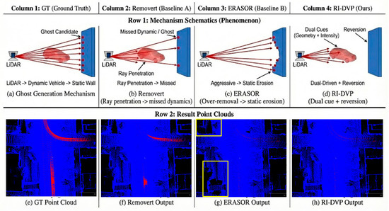
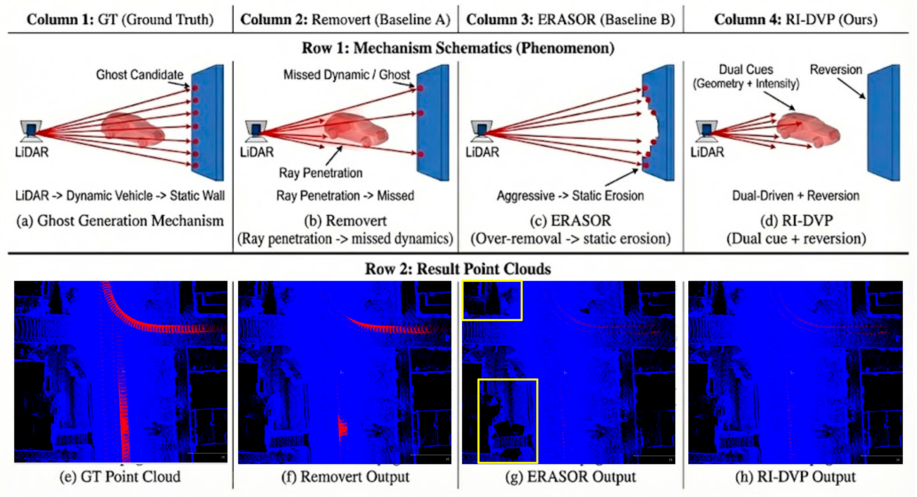
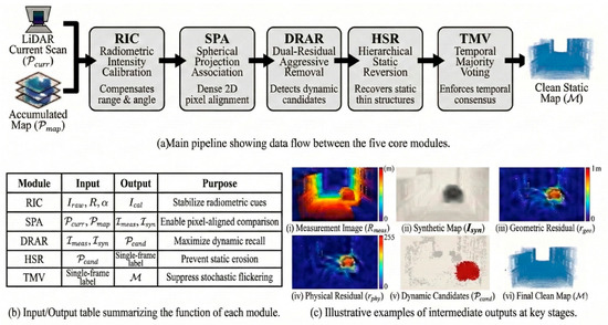
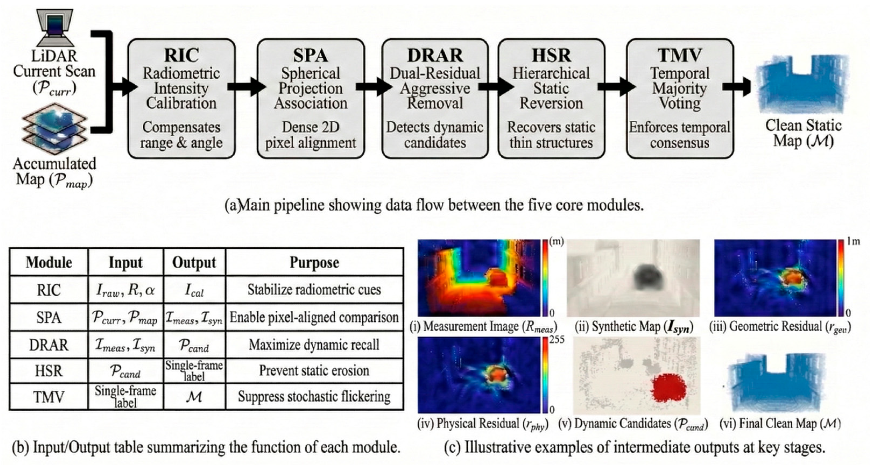
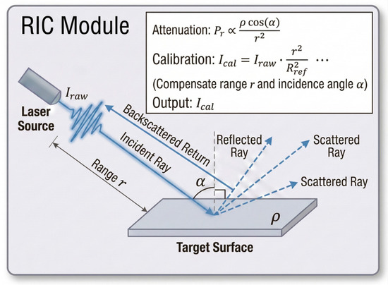
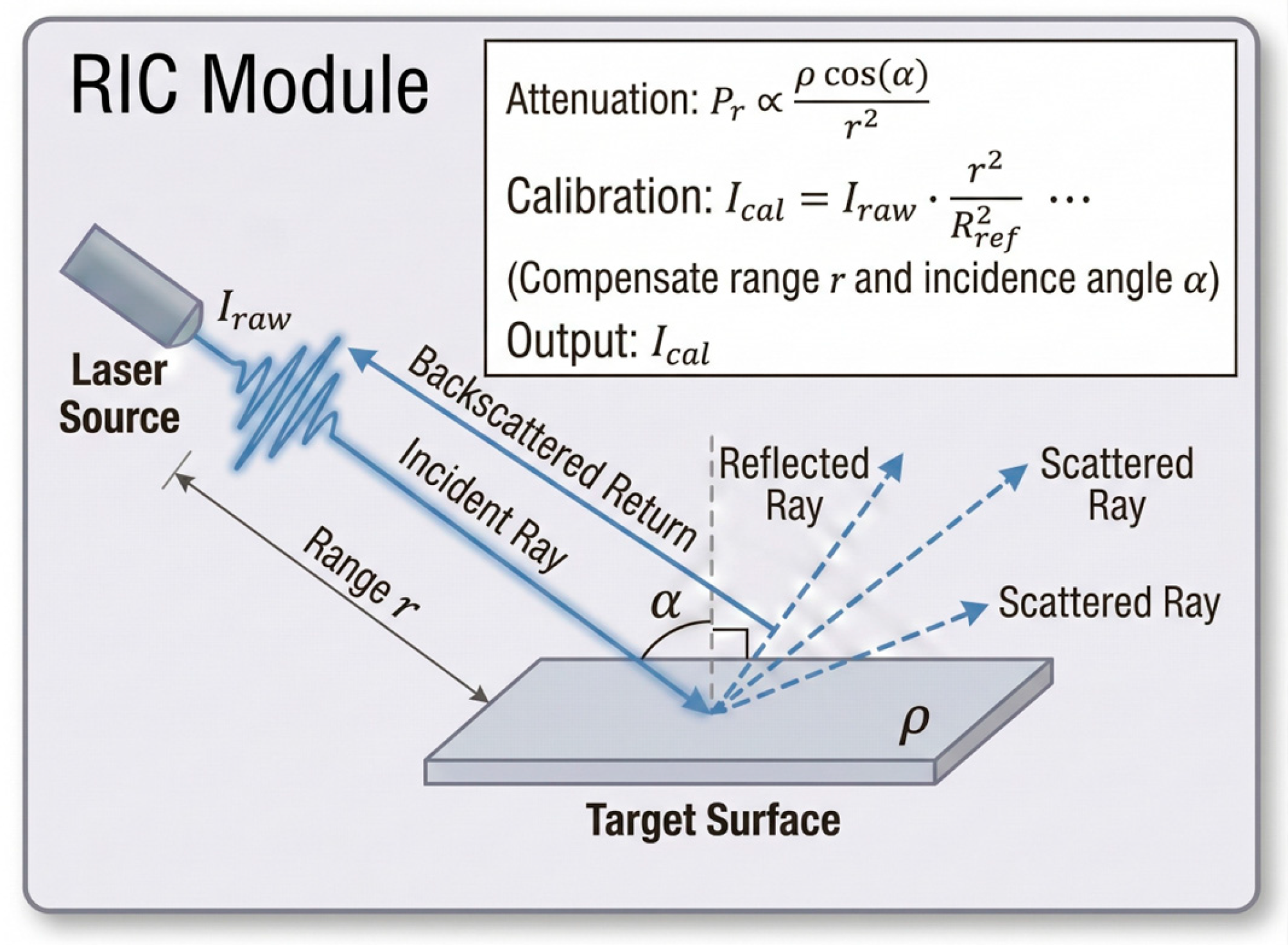
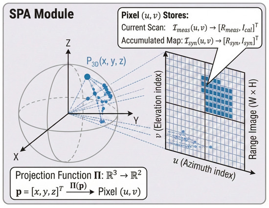
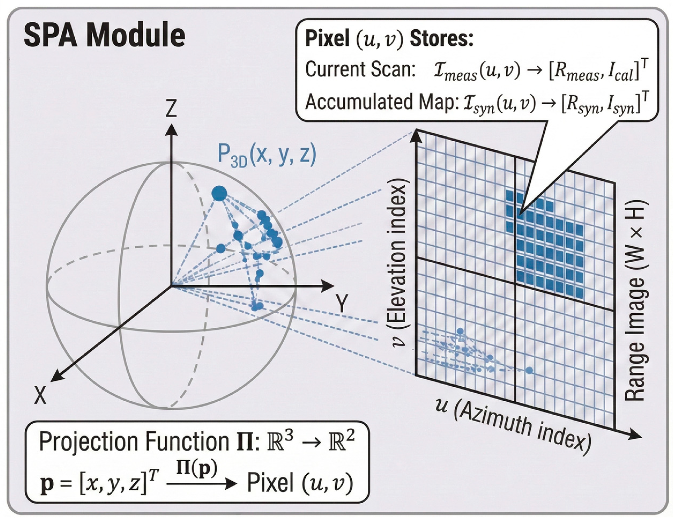
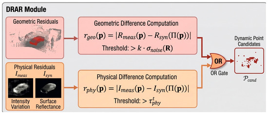
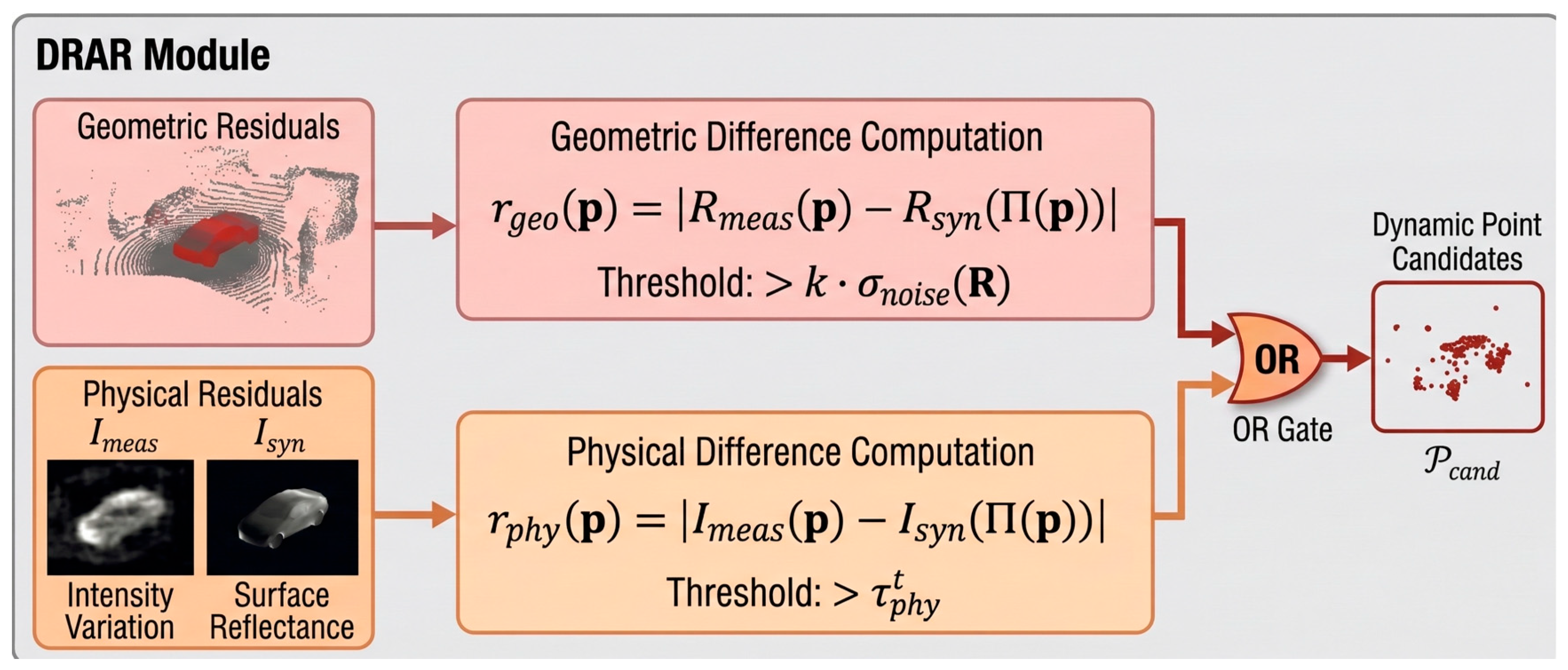
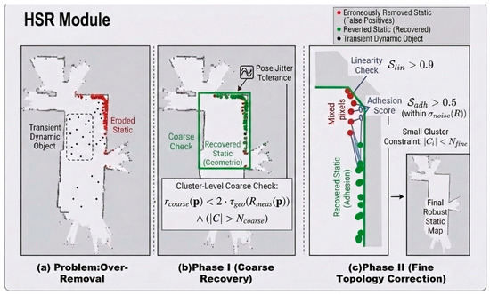
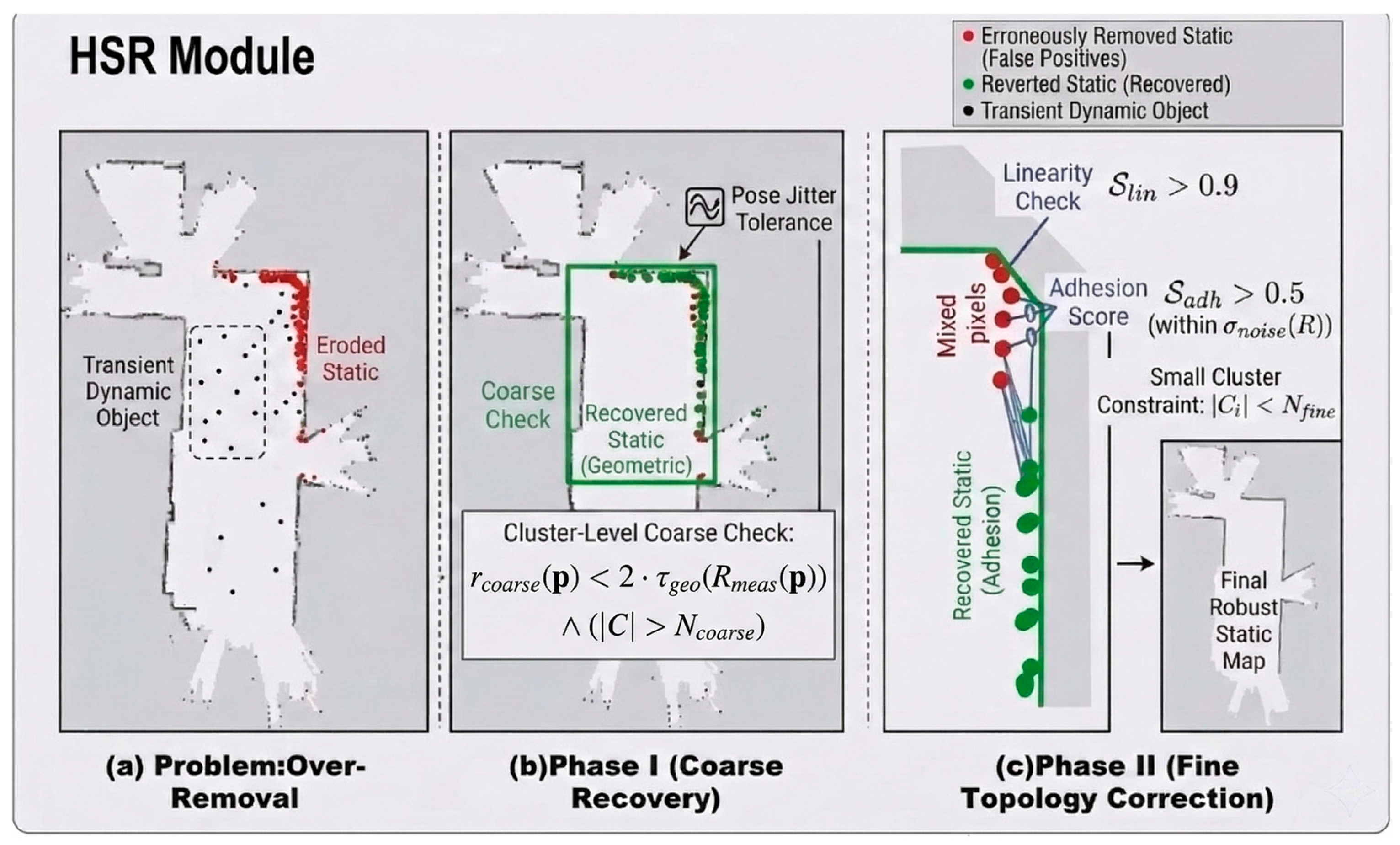
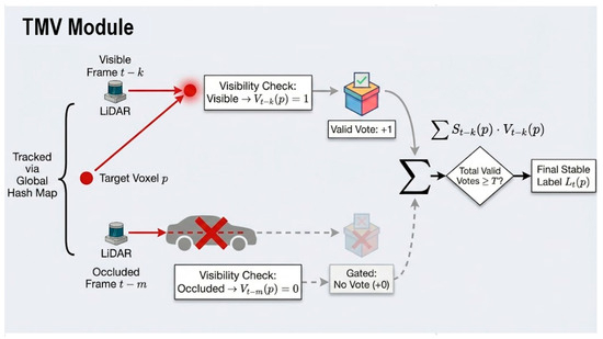
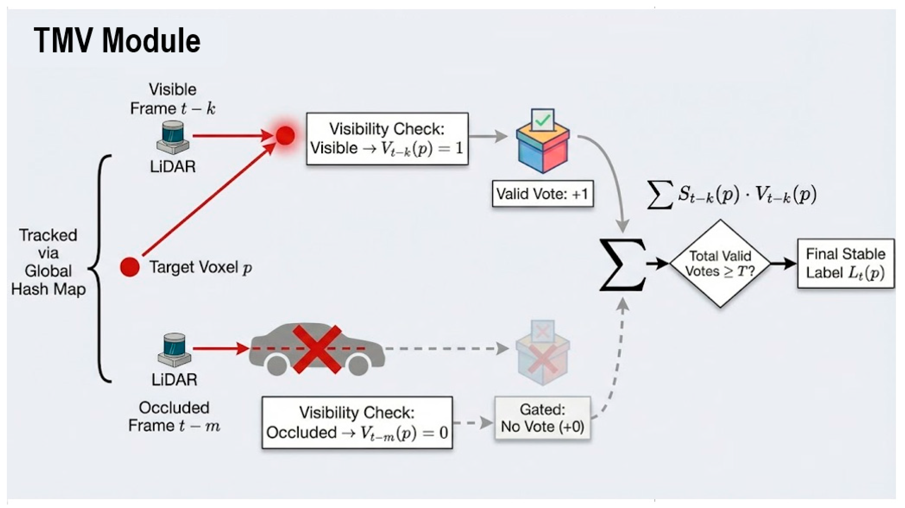
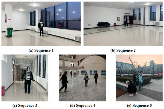
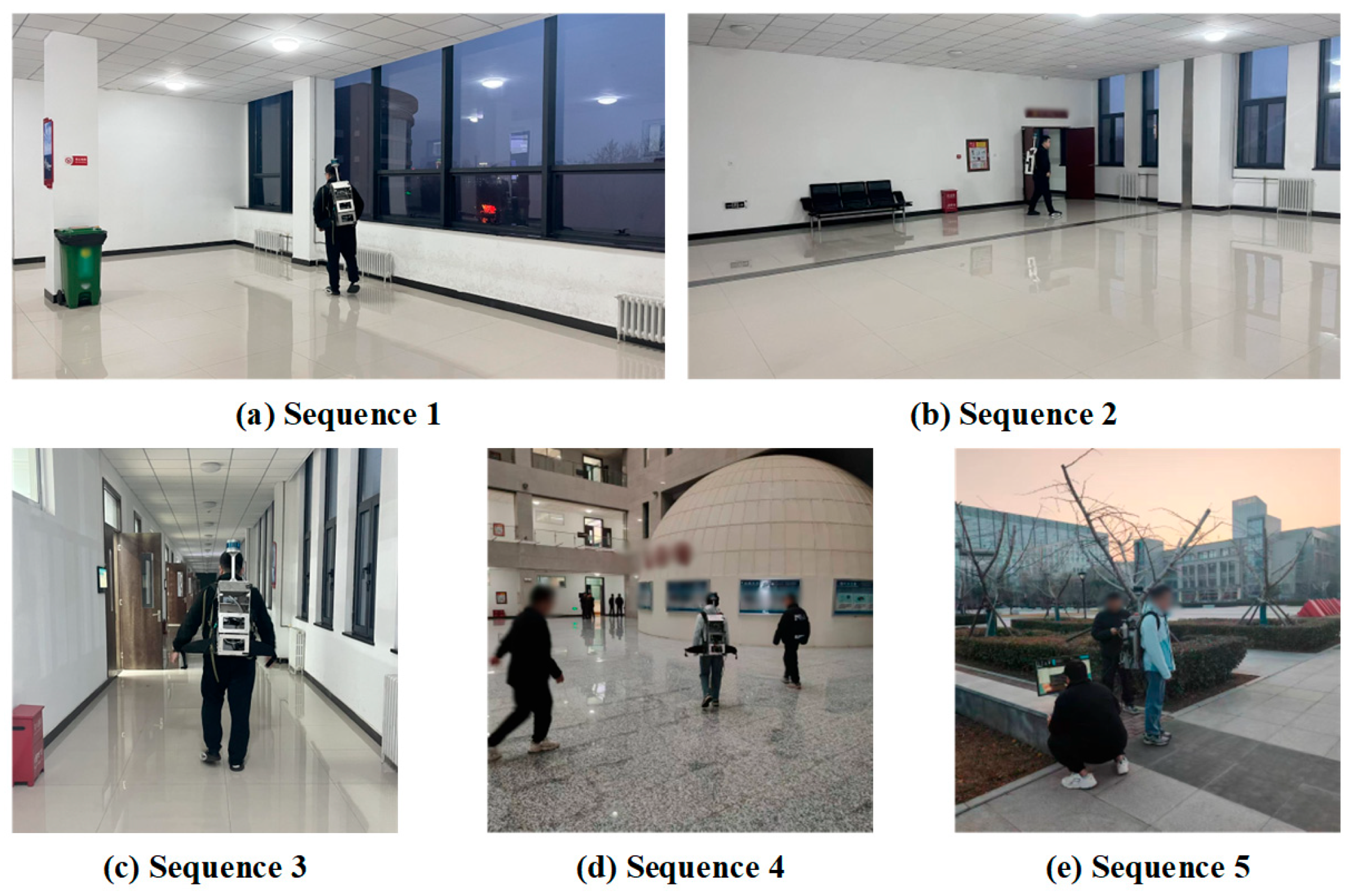
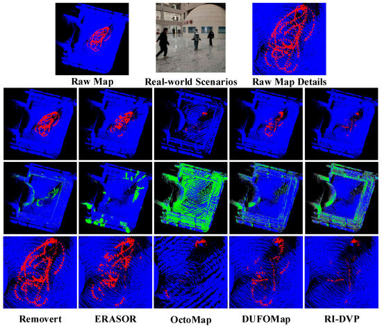
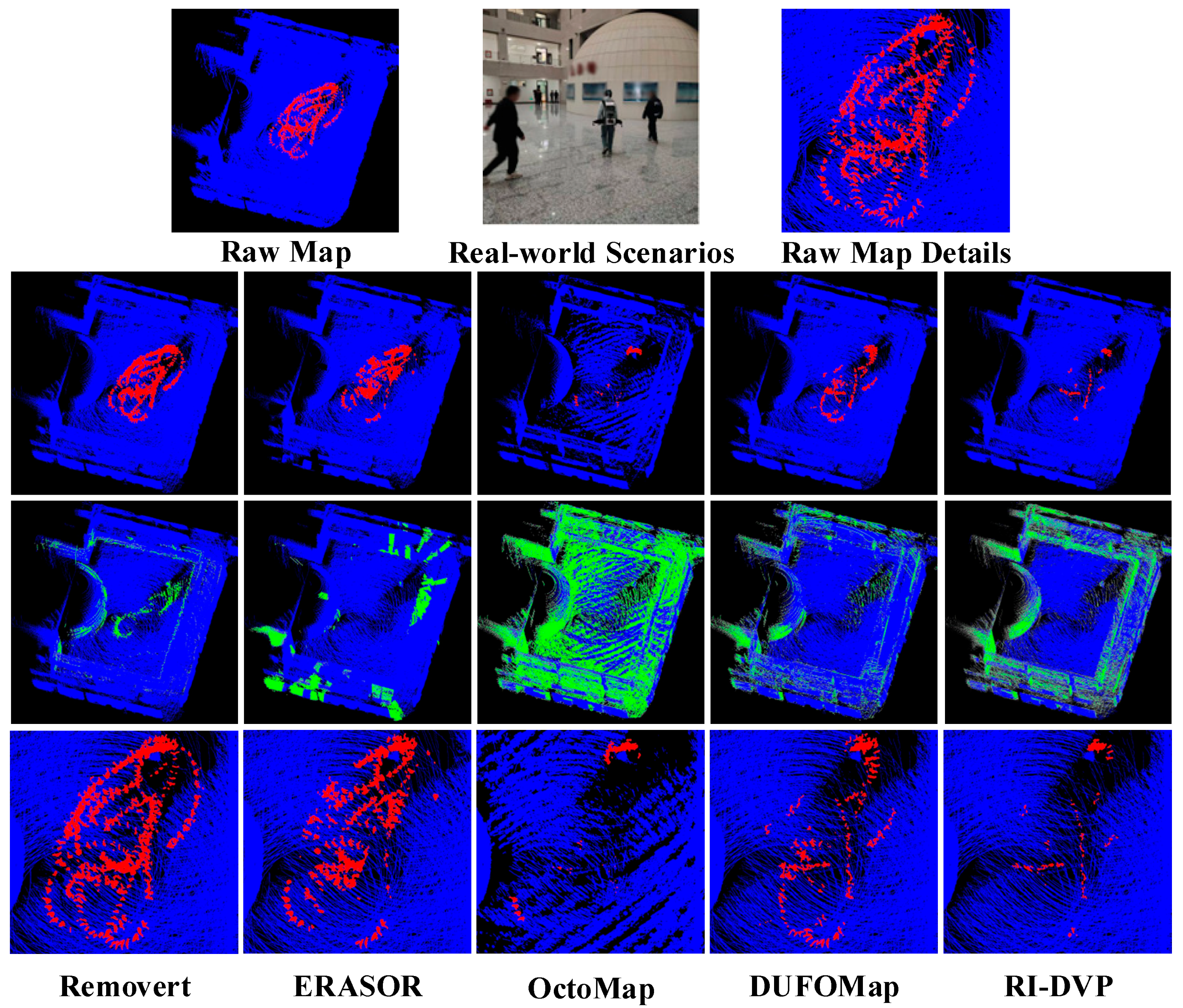
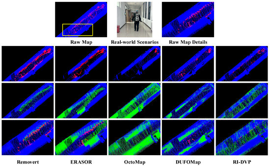
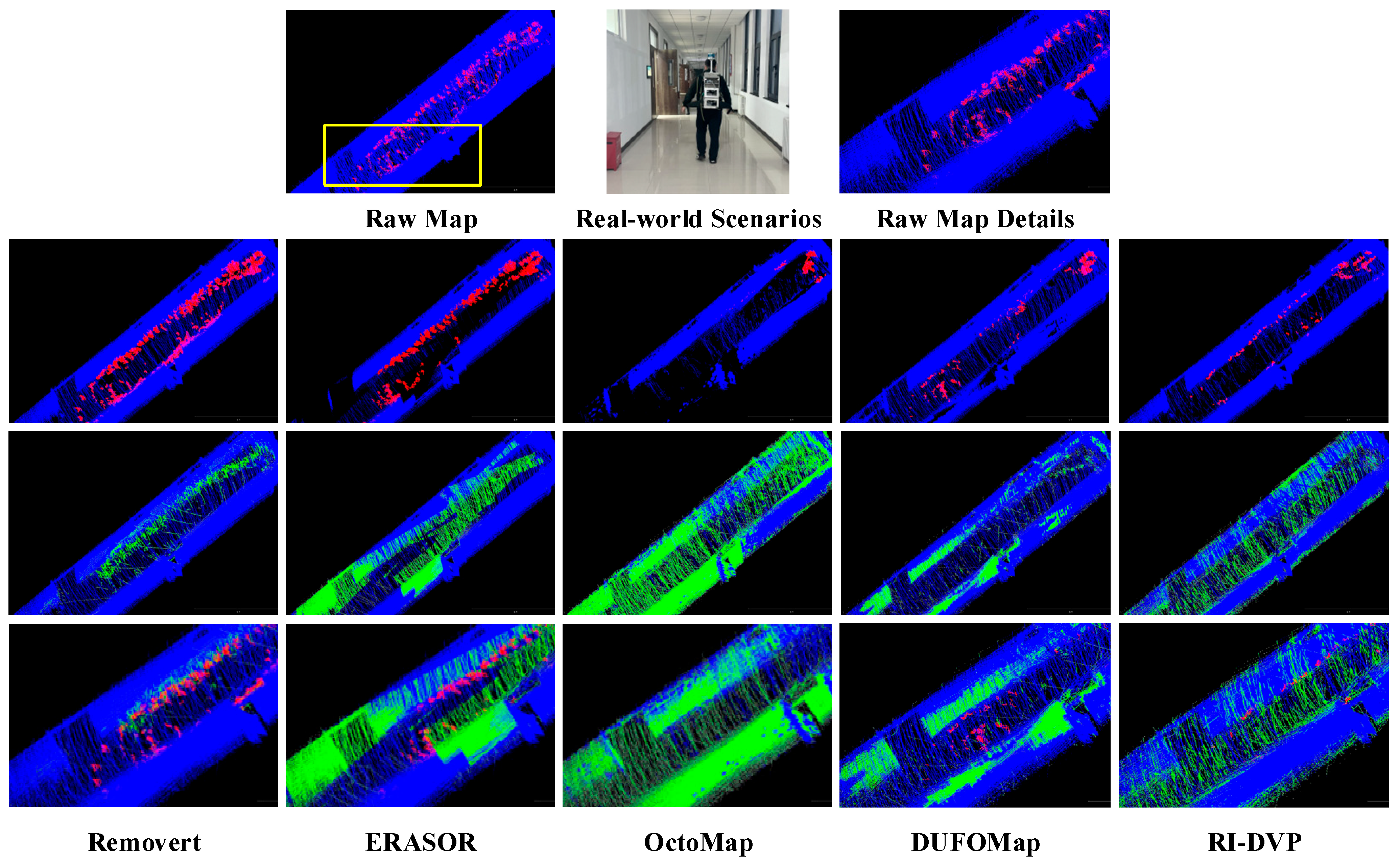
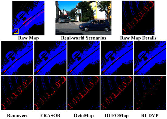
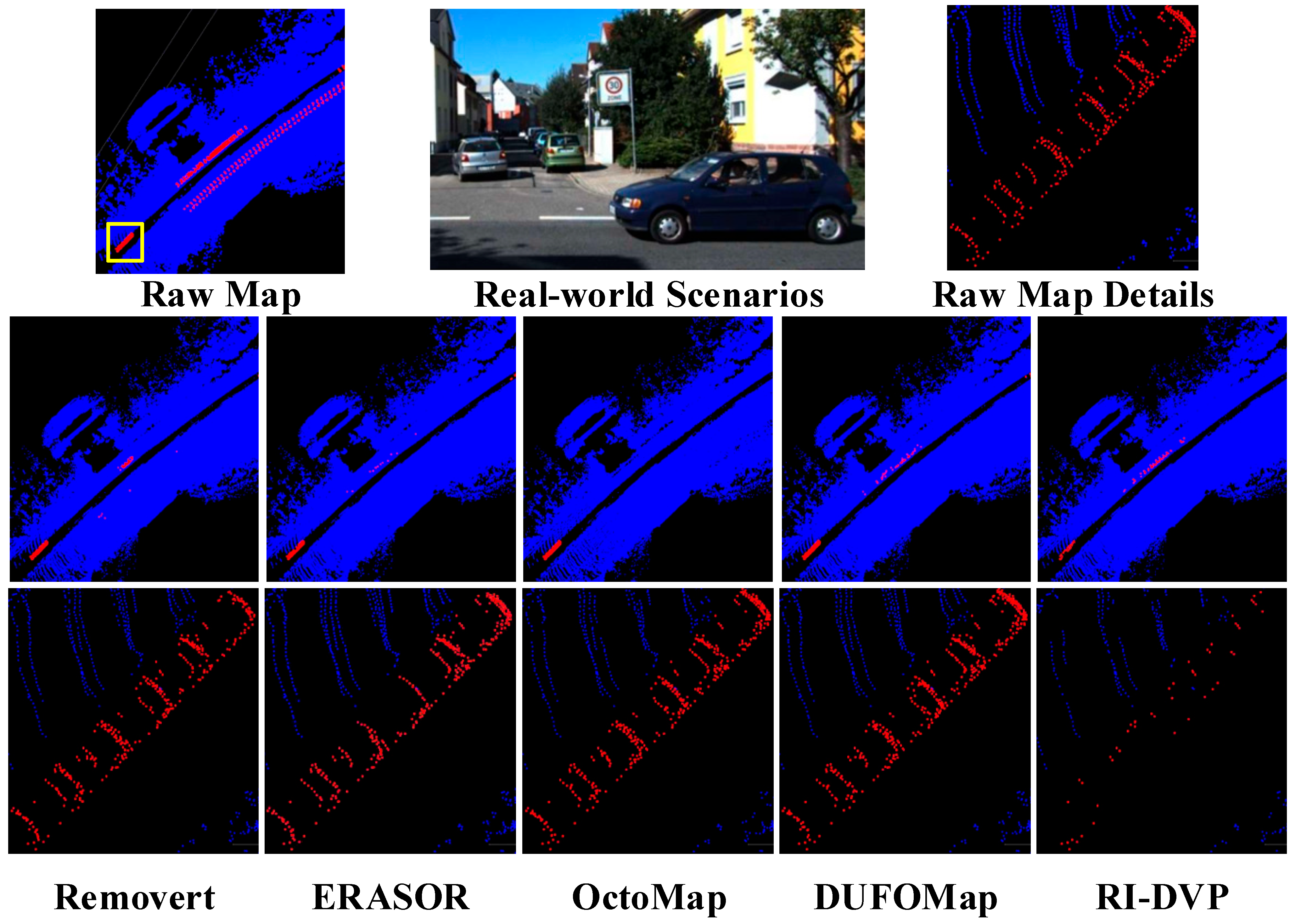

Disclaimer/Publisher’s Note: The statements, opinions and data contained in all publications are solely those of the individual author(s) and contributor(s) and not of MDPI and/or the editor(s). MDPI and/or the editor(s) disclaim responsibility for any injury to people or property resulting from any ideas, methods, instructions or products referred to in the content. |
© 2026 by the authors. Licensee MDPI, Basel, Switzerland. This article is an open access article distributed under the terms and conditions of the Creative Commons Attribution (CC BY) license.