Figure 1.
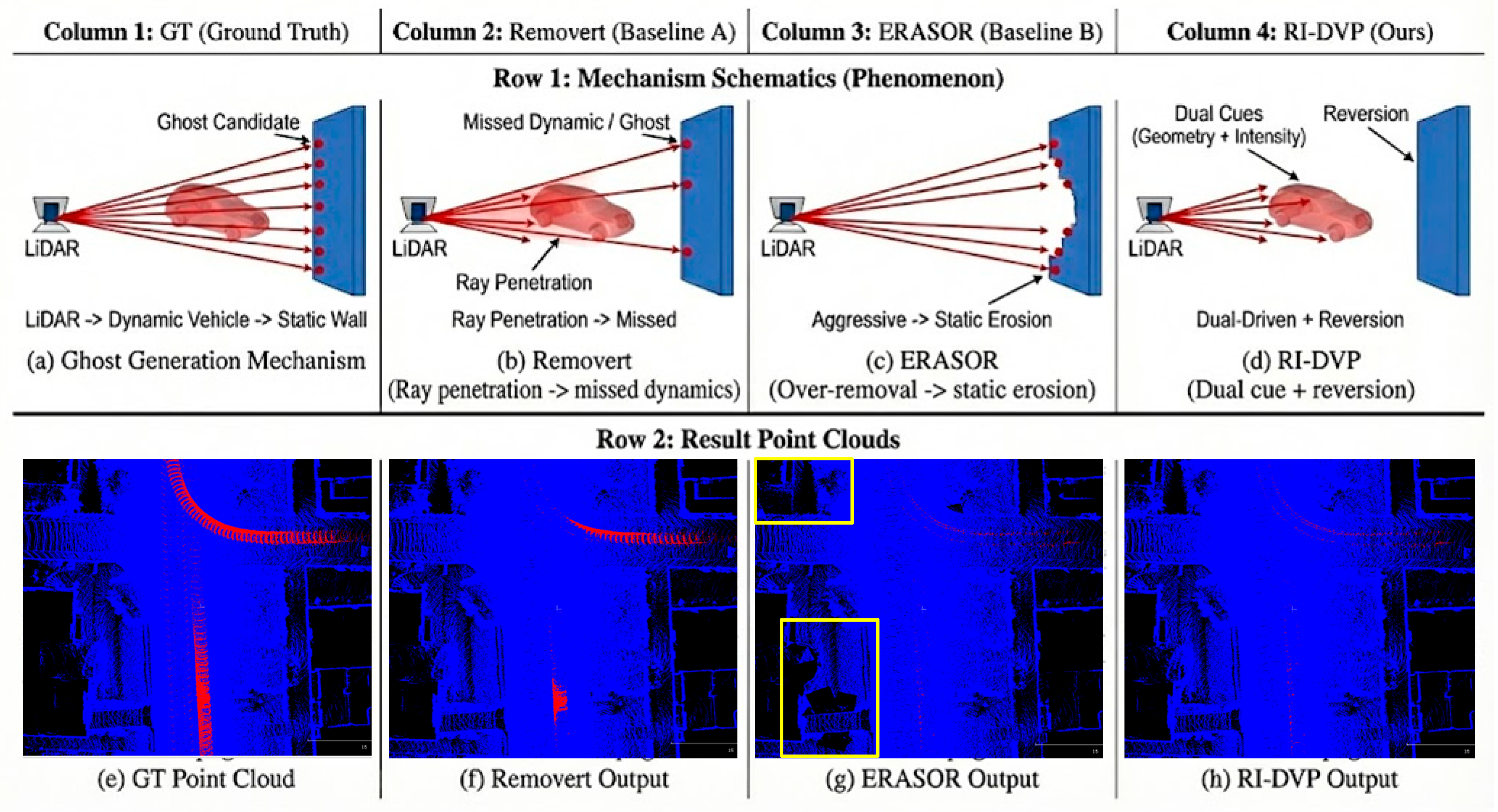
Illustration of the “Sparsity Trap” and qualitative comparison of dynamic artifact removal under sparse LiDAR observations. Top row: mechanism schematics. Bottom row: corresponding point-cloud results on the same scene/ROI and viewpoint. (a,e) Dynamic artifacts arise when sparse rays penetrate a moving object and hit the background, yielding spurious returns in the accumulated map; the GT visualization highlights the regions associated with dynamic artifacts (red). (b,f) A ray-visibility consistency baseline (Removert) may miss such subtle dynamics under sparse observability, leaving dynamic artifacts (red). (c,g) An aggressive geometric baseline (ERASOR) can over-remove points and erode valid static structures (static erosion, as indicated in the yellow box). (d,h) RI-DVP combines calibrated intensity cues with geometric consistency and a reversion step to suppress dynamic artifacts while preserving static scene geometry. Results are shown on SemanticKITTI sequence 05. Red denotes points associated with dynamic artifacts (or flagged/removed regions), and blue denotes retained static structure.
Figure 1.
Illustration of the “Sparsity Trap” and qualitative comparison of dynamic artifact removal under sparse LiDAR observations. Top row: mechanism schematics. Bottom row: corresponding point-cloud results on the same scene/ROI and viewpoint. (a,e) Dynamic artifacts arise when sparse rays penetrate a moving object and hit the background, yielding spurious returns in the accumulated map; the GT visualization highlights the regions associated with dynamic artifacts (red). (b,f) A ray-visibility consistency baseline (Removert) may miss such subtle dynamics under sparse observability, leaving dynamic artifacts (red). (c,g) An aggressive geometric baseline (ERASOR) can over-remove points and erode valid static structures (static erosion, as indicated in the yellow box). (d,h) RI-DVP combines calibrated intensity cues with geometric consistency and a reversion step to suppress dynamic artifacts while preserving static scene geometry. Results are shown on SemanticKITTI sequence 05. Red denotes points associated with dynamic artifacts (or flagged/removed regions), and blue denotes retained static structure.

Figure 2.
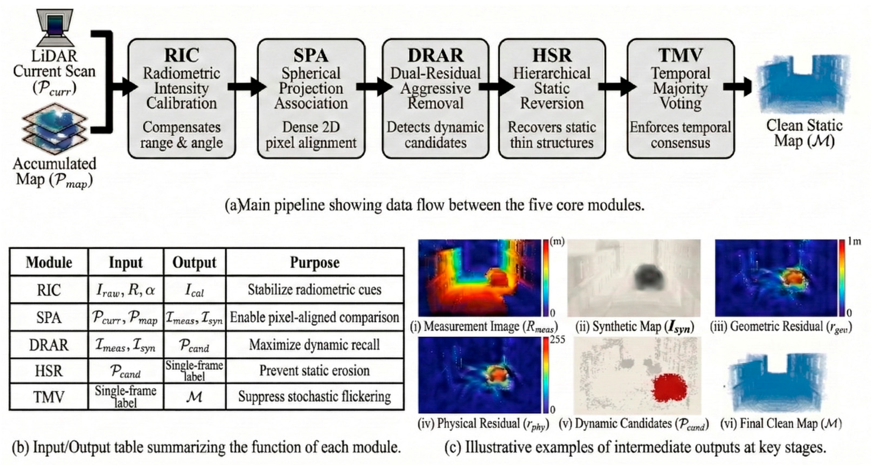
System overview of RI-DVP. (a) Main pipeline and data flow among the five modules: Radiometric Intensity Calibration (RIC), Spherical Projection Association (SPA), Dual-Residual Aggressive Removal (DRAR), Hierarchical Static Reversion (HSR), and Temporal Majority Voting (TMV). The inputs are the current scan and the accumulated map , and the output is the cleaned static map . (b) Input/output summary of each module. (c) Representative intermediate outputs, including the measurement/synthetic images, geometric and radiometric residual maps, dynamic candidates, and the final result. Examples are shown on Custom Sparse Dataset sequence 5.
Figure 2.
System overview of RI-DVP. (a) Main pipeline and data flow among the five modules: Radiometric Intensity Calibration (RIC), Spherical Projection Association (SPA), Dual-Residual Aggressive Removal (DRAR), Hierarchical Static Reversion (HSR), and Temporal Majority Voting (TMV). The inputs are the current scan and the accumulated map , and the output is the cleaned static map . (b) Input/output summary of each module. (c) Representative intermediate outputs, including the measurement/synthetic images, geometric and radiometric residual maps, dynamic candidates, and the final result. Examples are shown on Custom Sparse Dataset sequence 5.
Figure 3.
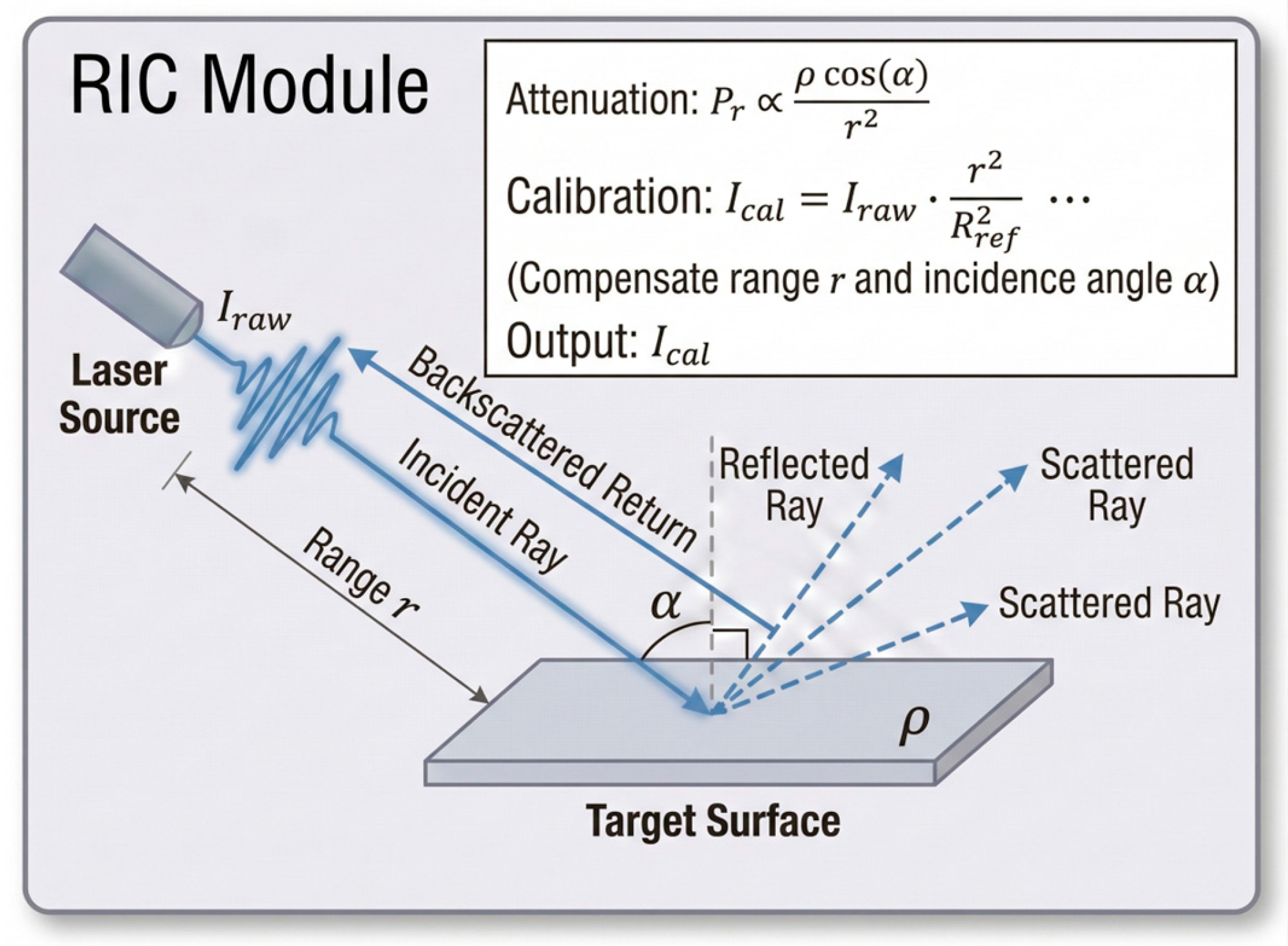
Schematic of the Radiometric Intensity Calibration (RIC) module. The raw LiDAR intensity () is inherently attenuated by the Euclidean range () and the incidence angle () relative to the surface normal. To obtain a more view-consistent intensity proxy related to surface reflectivity (), the RIC module employs a simplified radiometric model to compensate for these geometric variations, thereby outputting a radiometrically consistent intensity ().
Figure 3.
Schematic of the Radiometric Intensity Calibration (RIC) module. The raw LiDAR intensity () is inherently attenuated by the Euclidean range () and the incidence angle () relative to the surface normal. To obtain a more view-consistent intensity proxy related to surface reflectivity (), the RIC module employs a simplified radiometric model to compensate for these geometric variations, thereby outputting a radiometrically consistent intensity ().
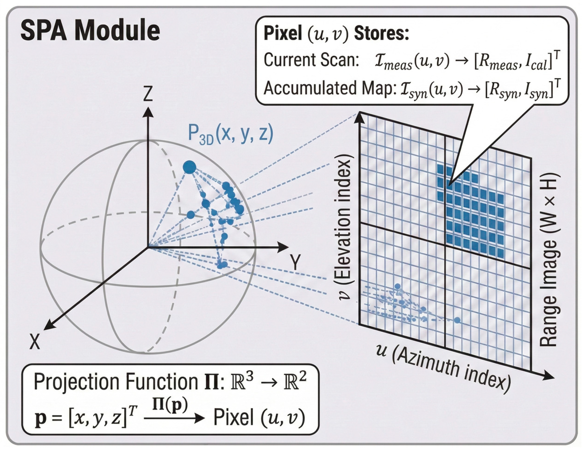
Figure 4.
Schematic of the Spherical Projection Association (SPA) module. To overcome the ambiguity of 3D nearest-neighbor searches in sparse point clouds, the SPA module defines a projection function that maps 3D points into 2D pixel grid indices . This structured representation enables the generation of two pixel-aligned images (Measurement Image and Synthetic Map Image ). Rather than storing spatial coordinates on the axes, each pixel directly stores the observed range and calibrated intensity, allowing for efficient dense-to-dense evaluation at the exact same line-of-sight.
Figure 4.
Schematic of the Spherical Projection Association (SPA) module. To overcome the ambiguity of 3D nearest-neighbor searches in sparse point clouds, the SPA module defines a projection function that maps 3D points into 2D pixel grid indices . This structured representation enables the generation of two pixel-aligned images (Measurement Image and Synthetic Map Image ). Rather than storing spatial coordinates on the axes, each pixel directly stores the observed range and calibrated intensity, allowing for efficient dense-to-dense evaluation at the exact same line-of-sight.
Figure 5.
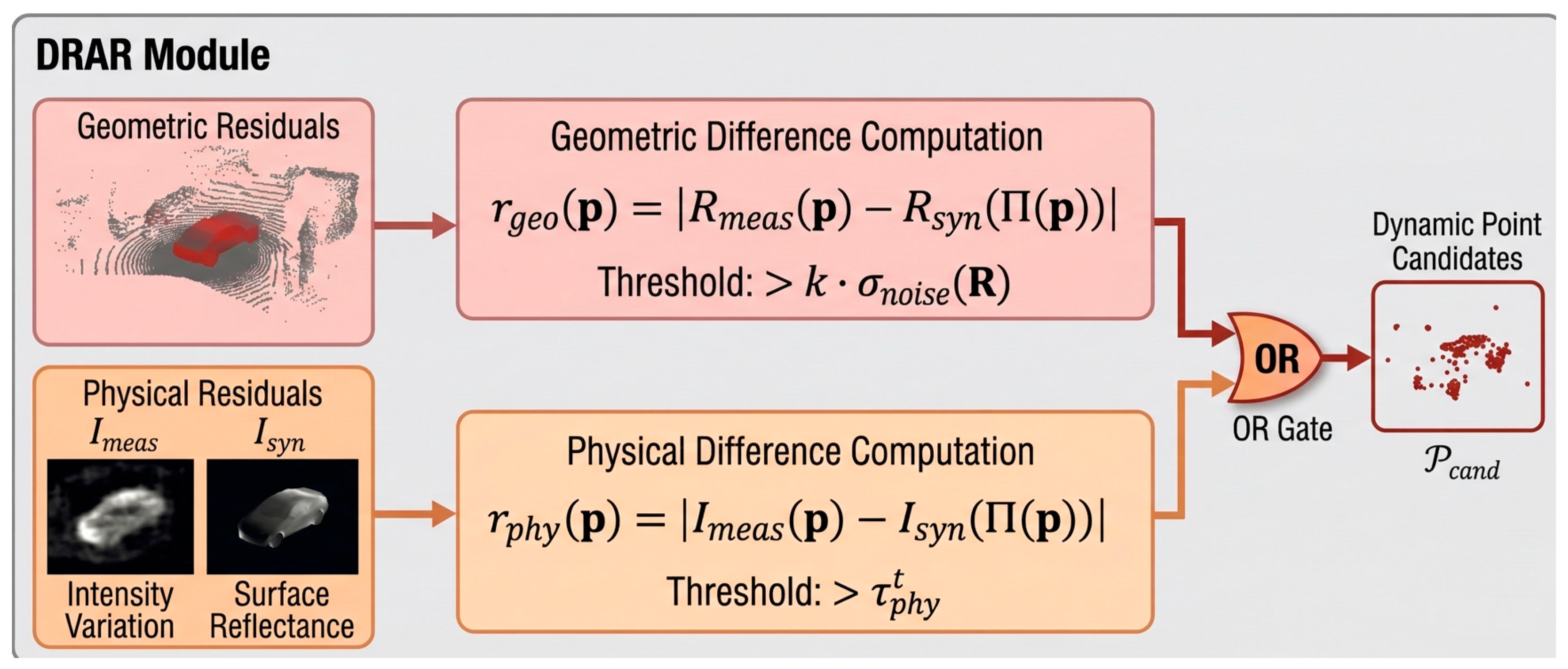
Schematic of the Dual-Residual Aggressive Removal (DRAR) module. Operating on pixel-aligned representations, the module computes two complementary metrics: the geometric residual () capturing spatial occupancy conflicts, and the physical residual () capturing material-level discrepancies. To mitigate the “Sparsity Trap” and boundary mixed-pixel effects, the geometric threshold incorporates a range-dependent spatial uncertainty envelope (). A logical OR gate combines these criteria, prioritizing recall by outputting Candidate Dynamic Points () if a significant anomaly is detected in either the structural or material domain. (Note: For clarity, the pixel association projection is omitted in the schematic formulas; the full rigorous formulation is detailed in Equations (6) and (7). The red point cloud represents the dynamic candidate point cloud.).
Figure 5.
Schematic of the Dual-Residual Aggressive Removal (DRAR) module. Operating on pixel-aligned representations, the module computes two complementary metrics: the geometric residual () capturing spatial occupancy conflicts, and the physical residual () capturing material-level discrepancies. To mitigate the “Sparsity Trap” and boundary mixed-pixel effects, the geometric threshold incorporates a range-dependent spatial uncertainty envelope (). A logical OR gate combines these criteria, prioritizing recall by outputting Candidate Dynamic Points () if a significant anomaly is detected in either the structural or material domain. (Note: For clarity, the pixel association projection is omitted in the schematic formulas; the full rigorous formulation is detailed in Equations (6) and (7). The red point cloud represents the dynamic candidate point cloud.).
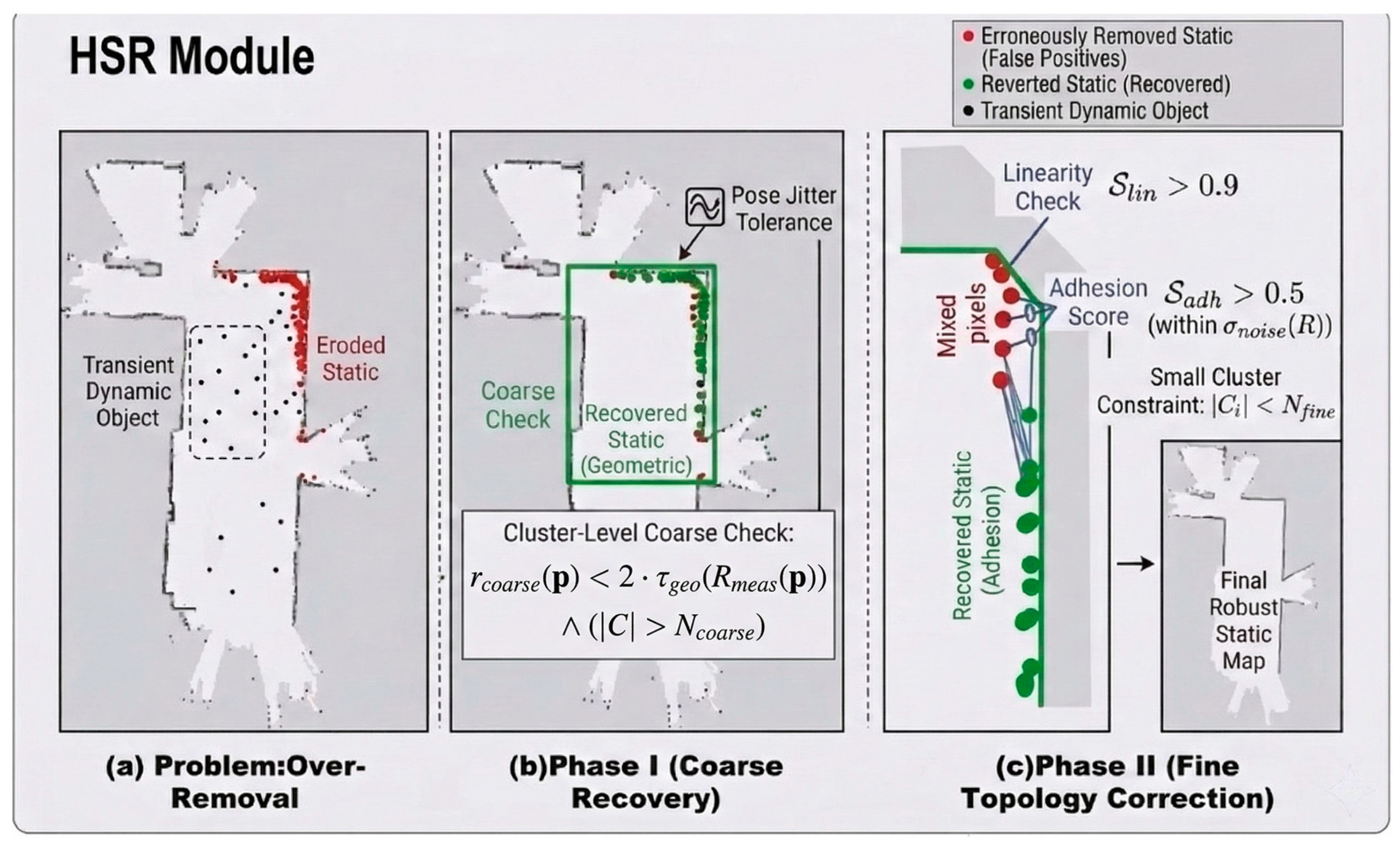
Figure 6.
Schematic of the Hierarchical Static Reversion (HSR) Mechanism. (a) Problem: Aggressive dynamic removal inherently causes static erosion (red points, false positives) due to minor pose jitter and mixed-pixel artifacts around static boundaries. The dashed box indicates the transient dynamic object. (b) Phase I (Coarse Recovery): Taking the dynamic candidates (from DRAR) as input, a coarse-scale geometric check leverages reduced-resolution visibility to tolerate pose errors. Points are reverted if their coarse residual is within a relaxed threshold and they belong to a large cluster (), recovering bulk static structures. (c) Phase II (Fine Topology Correction): Taking the remaining unrecovered candidates from Phase I as input, a fine-scale topology-based correction identifies subtle edge artifacts. Points are recovered only if they form small clusters (), exhibit high linearity (), and are structurally “adhered” to the recovered static map () within a local proximity radius .
Figure 6.
Schematic of the Hierarchical Static Reversion (HSR) Mechanism. (a) Problem: Aggressive dynamic removal inherently causes static erosion (red points, false positives) due to minor pose jitter and mixed-pixel artifacts around static boundaries. The dashed box indicates the transient dynamic object. (b) Phase I (Coarse Recovery): Taking the dynamic candidates (from DRAR) as input, a coarse-scale geometric check leverages reduced-resolution visibility to tolerate pose errors. Points are reverted if their coarse residual is within a relaxed threshold and they belong to a large cluster (), recovering bulk static structures. (c) Phase II (Fine Topology Correction): Taking the remaining unrecovered candidates from Phase I as input, a fine-scale topology-based correction identifies subtle edge artifacts. Points are recovered only if they form small clusters (), exhibit high linearity (), and are structurally “adhered” to the recovered static map () within a local proximity radius .

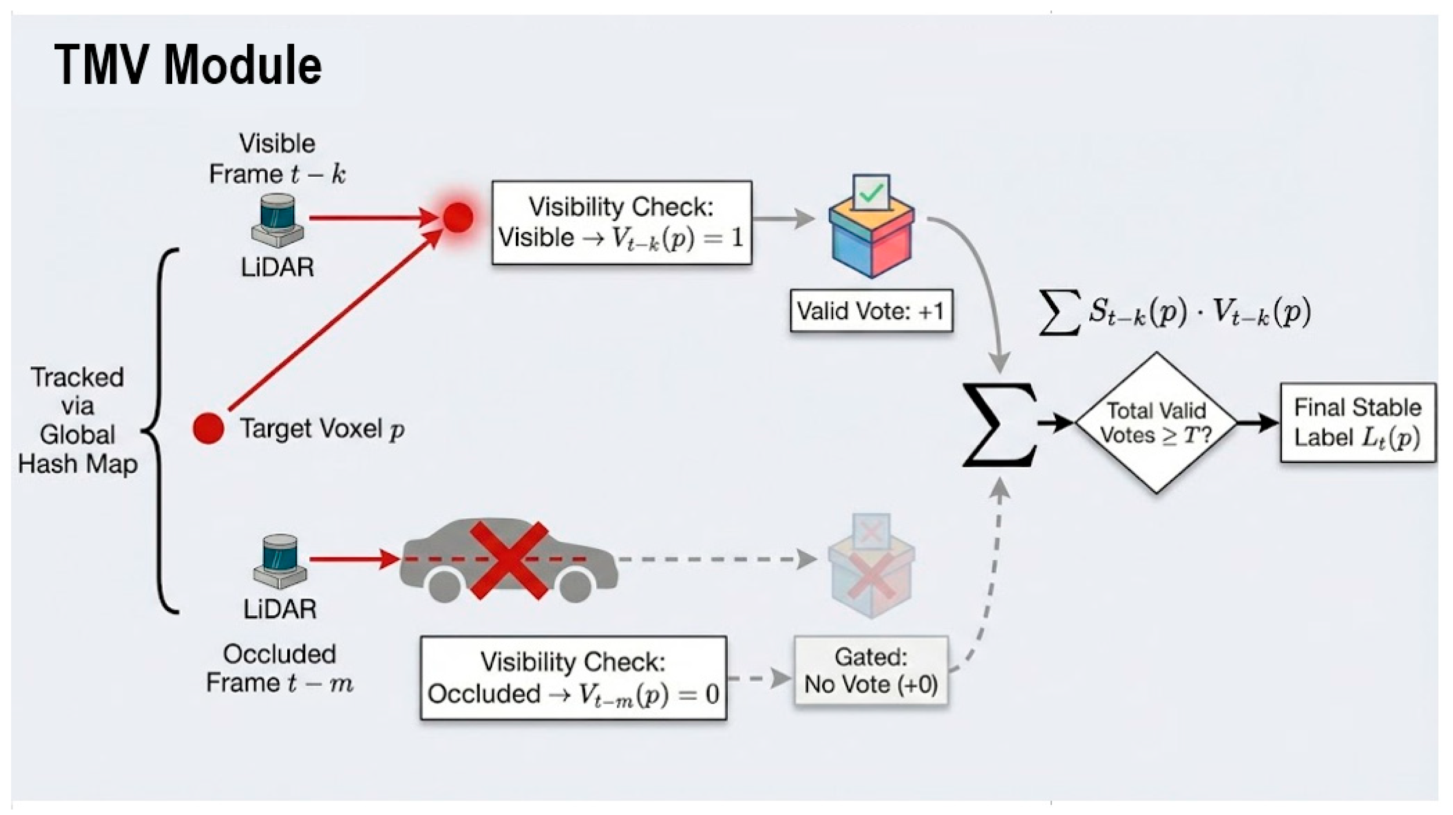
Figure 7.
Schematic of the TMV Module with Visibility-Gated Sliding Window. The framework tracks the historical states of spatial voxels (indexed via global hash map) over a sliding window. To ensure reliability against occlusion, a visibility gating mechanism evaluates ray-casting connectivity. If target voxel is physically occluded in a past frame (e.g., by a vehicle in Frame ), its contribution is gated (, No Vote). Only visible observations () contribute to the accumulated vote count , which is then thresholded against to determine the final stable label . The solid red arrow indicates the visible line-of-sight from the LiDAR to the target voxel, while the dashed grey arrow denotes the occluded path blocked by a dynamic object.
Figure 7.
Schematic of the TMV Module with Visibility-Gated Sliding Window. The framework tracks the historical states of spatial voxels (indexed via global hash map) over a sliding window. To ensure reliability against occlusion, a visibility gating mechanism evaluates ray-casting connectivity. If target voxel is physically occluded in a past frame (e.g., by a vehicle in Frame ), its contribution is gated (, No Vote). Only visible observations () contribute to the accumulated vote count , which is then thresholded against to determine the final stable label . The solid red arrow indicates the visible line-of-sight from the LiDAR to the target voxel, while the dashed grey arrow denotes the occluded path blocked by a dynamic object.
Figure 8.
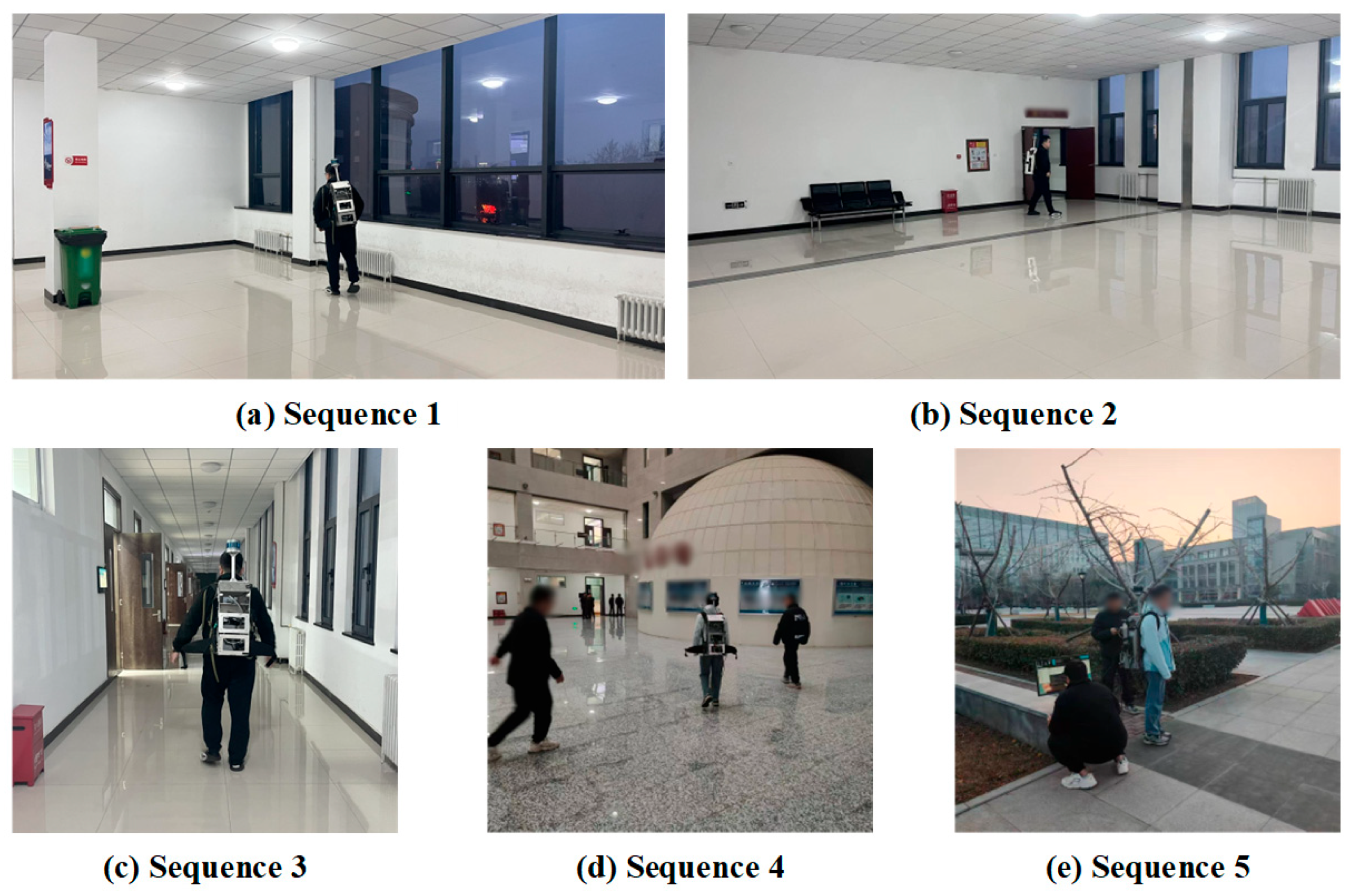
Representative real-world data collection scenarios for the custom VLP-16 sparse dataset. (a,b) Indoor structured spaces (Sequences 1 and 2), providing complex static geometries to evaluate structural preservation. (c) A structured narrow corridor (Sequence 3), which is highly prone to grazing-incidence errors. (d) An indoor open lobby (Sequence 4) presenting severe geometric registration degeneracies due to sparse far-range returns. (e) An outdoor unstructured campus (Sequence 5) featuring large-scale sparse surroundings.
Figure 8.
Representative real-world data collection scenarios for the custom VLP-16 sparse dataset. (a,b) Indoor structured spaces (Sequences 1 and 2), providing complex static geometries to evaluate structural preservation. (c) A structured narrow corridor (Sequence 3), which is highly prone to grazing-incidence errors. (d) An indoor open lobby (Sequence 4) presenting severe geometric registration degeneracies due to sparse far-range returns. (e) An outdoor unstructured campus (Sequence 5) featuring large-scale sparse surroundings.
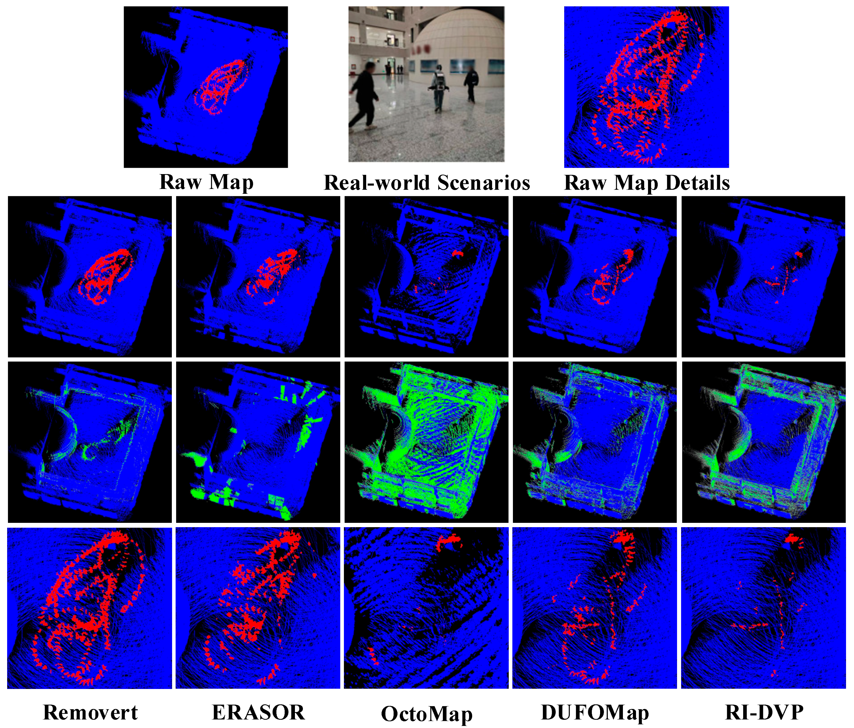
Figure 9.
Qualitative evaluation of dynamic artifact removal in an indoor open environment (Custom Seq 4). Row 1 displays the raw map, the corresponding real-world scenario, and magnified details of the dynamic artifacts, respectively. Row 2 presents the global views of the dynamic artifacts identification results across five algorithms, while Row 3 illustrates the static information loss (erroneously removed static points, typically highlighted in green) in the global view. Row 4 provides magnified details of the dynamic artifacts identification results for each method. In the point clouds, preserved static structures are colored blue, and removed dynamic points are colored red.
Figure 9.
Qualitative evaluation of dynamic artifact removal in an indoor open environment (Custom Seq 4). Row 1 displays the raw map, the corresponding real-world scenario, and magnified details of the dynamic artifacts, respectively. Row 2 presents the global views of the dynamic artifacts identification results across five algorithms, while Row 3 illustrates the static information loss (erroneously removed static points, typically highlighted in green) in the global view. Row 4 provides magnified details of the dynamic artifacts identification results for each method. In the point clouds, preserved static structures are colored blue, and removed dynamic points are colored red.
Figure 10.
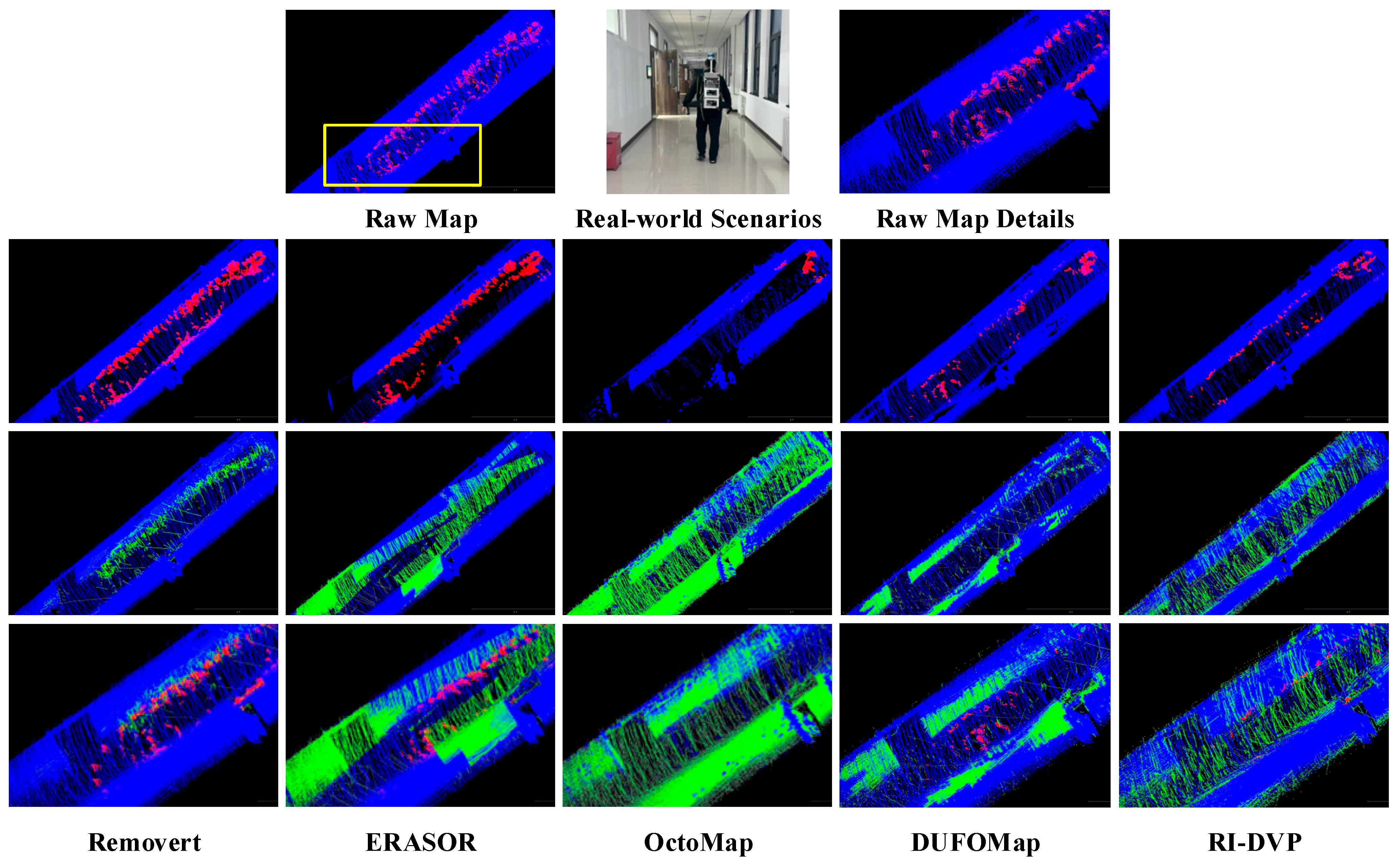
Qualitative evaluation of static structure preservation in a narrow corridor environment (Custom Seq 3). Row 1 presents the raw map, the corresponding real-world scenario, and a magnified view of the key regions of interest (ROIs) within the raw map, as highlighted by the yellow box. Row 2 illustrates the global views of the dynamic artifacts identification results across five algorithms. Row 3 highlights the static information loss in the global view, demonstrating the extent of static erosion (e.g., on walls or floors). Row 4 presents the corresponding map details for the five algorithms to compare their structural preservation capabilities. Preserved static points are indicated in blue, and identified dynamic artifacts are in red, while green points represent static points that were erroneously removed.
Figure 10.
Qualitative evaluation of static structure preservation in a narrow corridor environment (Custom Seq 3). Row 1 presents the raw map, the corresponding real-world scenario, and a magnified view of the key regions of interest (ROIs) within the raw map, as highlighted by the yellow box. Row 2 illustrates the global views of the dynamic artifacts identification results across five algorithms. Row 3 highlights the static information loss in the global view, demonstrating the extent of static erosion (e.g., on walls or floors). Row 4 presents the corresponding map details for the five algorithms to compare their structural preservation capabilities. Preserved static points are indicated in blue, and identified dynamic artifacts are in red, while green points represent static points that were erroneously removed.
Figure 11.
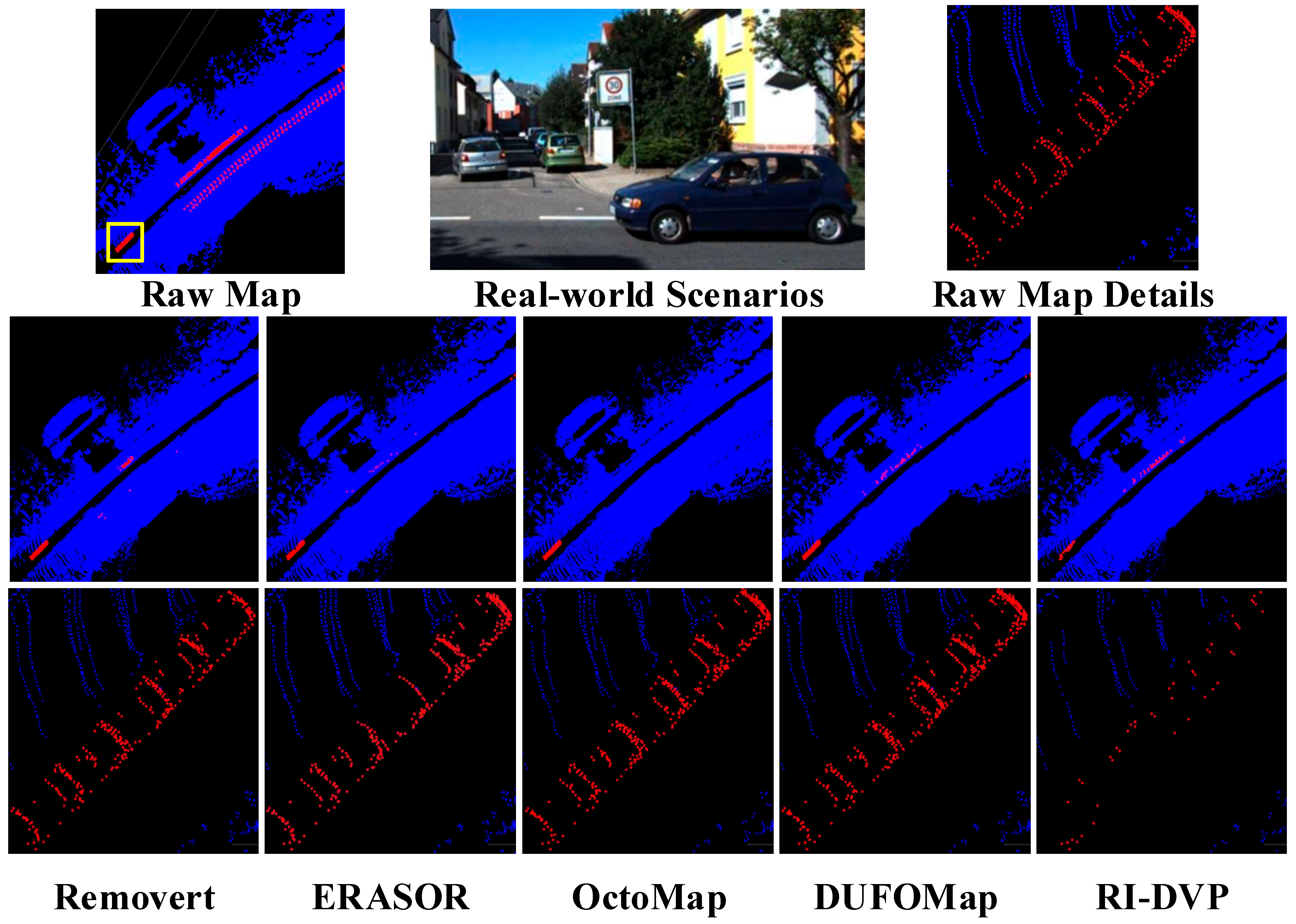
Qualitative evaluation of resolving geometric ambiguity in a highway scenario (SemanticKITTI Seq 01). Row 1 presents the raw map, the corresponding real-world scenario, and a magnified view of the key regions of interest (ROIs) highlighted by the yellow box, which specifically represent sparse dynamic artifacts located at the map boundaries. Row 2 presents the global views of the dynamic artifacts identification results across five algorithms. Row 3 details the specific identification and removal performance targeting the sparse dynamic artifacts at the map edge. The preserved static background is denoted in blue, while the red points correspond to the identified dynamic artifacts.
Figure 11.
Qualitative evaluation of resolving geometric ambiguity in a highway scenario (SemanticKITTI Seq 01). Row 1 presents the raw map, the corresponding real-world scenario, and a magnified view of the key regions of interest (ROIs) highlighted by the yellow box, which specifically represent sparse dynamic artifacts located at the map boundaries. Row 2 presents the global views of the dynamic artifacts identification results across five algorithms. Row 3 details the specific identification and removal performance targeting the sparse dynamic artifacts at the map edge. The preserved static background is denoted in blue, while the red points correspond to the identified dynamic artifacts.
Table 1.
Quantitative results on SemanticKITTI (Urban/Highway Scenarios).
Table 1.
Quantitative results on SemanticKITTI (Urban/Highway Scenarios).
| Methods | 00: Urban Area | 01: Highway | 07: Urban Intersection |
|---|
| SA | DA | AA | SA | DA | AA | SA | DA | AA |
|---|
| Removert | 99.44 | 41.53 | 64.26 | 98.38 | 41.50 | 63.90 | 99.80 | 28.56 | 53.39 |
| ERASOR | 66.70 | 98.54 | 81.07 | 98.38 | 91.95 | 95.11 | 67.10 | 86.18 | 76.04 |
| OctoMap | 68.05 | 99.69 | 82.36 | 57.34 | 99.29 | 75.45 | 85.45 | 87.39 | 86.41 |
| DUFOMap | 99.70 | 89.92 | 94.68 | 93.89 | 91.51 | 92.69 | 96.84 | 80.81 | 88.46 |
| RI-DVP | 87.14 | 98.45 | 92.62 | 84.56 | 96.01 | 90.10 | 93.69 | 84.99 | 89.36 |
Table 2.
Quantitative results on SemanticKITTI (Rural/Unstructured Scenarios).
Table 2.
Quantitative results on SemanticKITTI (Rural/Unstructured Scenarios).
| Methods | 02: Rural T-Junction | 05: Rural Area | 09: Rural Road |
|---|
| SA | DA | AA | SA | DA | AA | SA | DA | AA |
|---|
| Removert | 97.34 | 40.88 | 63.08 | 99.42 | 22.28 | 47.06 | 99.25 | 43.37 | 65.61 |
| ERASOR | 47.48 | 93.28 | 66.55 | 69.40 | 99.06 | 82.91 | 89.05 | 86.20 | 87.61 |
| OctoMap | 60.86 | 97.38 | 76.98 | 66.28 | 99.24 | 81.10 | 76.70 | 90.96 | 83.52 |
| DUFOMap | 72.14 | 89.79 | 80.48 | 95.31 | 87.86 | 91.51 | 96.09 | 82.05 | 88.79 |
| RI-DVP | 79.87 | 93.35 | 86.35 | 87.44 | 97.95 | 92.55 | 87.75 | 91.76 | 89.73 |
Table 3.
Quantitative evaluation on sparse scenarios (Structured Narrow Environment).
Table 3.
Quantitative evaluation on sparse scenarios (Structured Narrow Environment).
| Methods | Seq 1: Indoor Structured Narrow Space | Seq 2: Indoor Structured Space | Seq 3: Structured Narrow Long Corridor |
|---|
| SA | DA | AA | SA | DA | AA | SA | DA | AA |
|---|
| Removert | 99.18 | 17.95 | 42.20 | 99.19 | 12.49 | 35.20 | 99.52 | 10.33 | 32.06 |
| ERASOR | 96.36 | 57.42 | 74.38 | 85.71 | 72.11 | 79.44 | 87.61 | 45.41 | 63.07 |
| OctoMap | 80.27 | 95.29 | 87.46 | 81.51 | 94.38 | 87.71 | 71.81 | 88.72 | 79.82 |
| DUFOMap | 95.51 | 80.94 | 87.92 | 97.36 | 61.76 | 77.54 | 95.49 | 57.13 | 73.86 |
| RI-DVP | 93.30 | 86.45 | 89.81 | 95.46 | 80.69 | 87.76 | 97.76 | 74.11 | 85.12 |
Table 4.
Quantitative evaluation on sparse scenarios (Open Environments).
Table 4.
Quantitative evaluation on sparse scenarios (Open Environments).
| Methods | Seq 4: Indoor Open Space | Seq 5: Outdoor Open Space |
|---|
| SA | DA | AA | SA | DA | AA |
|---|
| Removert | 99.49 | 24.31 | 49.18 | 99.40 | 18.49 | 42.87 |
| ERASOR | 94.38 | 38.45 | 60.24 | 96.41 | 62.04 | 77.34 |
| OctoMap | 76.7 | 88.50 | 82.39 | 74.84 | 92.00 | 82.98 |
| DUFOMap | 95.37 | 78.78 | 86.68 | 96.26 | 50.23 | 69.54 |
| RI-DVP | 87.49 | 89.50 | 88.49 | 83.13 | 87.06 | 85.07 |
Table 5.
Ablation study on Custom Seq 4.
Table 5.
Ablation study on Custom Seq 4.
| Methods | Seq 4: Indoor Open Space |
|---|
| SA | DA | AA |
|---|
| Baseline | 95.15 | 41.21 | 62.61 |
| Aggressive | 78.42 | 91.05 | 84.50 |
| Proposed | 87.49 | 89.50 | 88.49 |
Table 6.
Average runtime comparison (ms/frame).
Table 6.
Average runtime comparison (ms/frame).
| Methods | Seq 01 (64-Beam) | Seq 1 (16-Beam) |
|---|
| High Load | Real-Time Scenario |
|---|
| Removert | 555.32 | 166.42 |
| ERASOR | 390.75 | 23.12 |
| OctoMap | 1234.68 | 222.29 |
| DUFOMap | 80.93 | 24.42 |
| RI-DVP | 288.56 | 65.40 |
Table 7.
Influence of pose source on dynamic-removal performance in Custom Seq 1 (Indoor Structured Narrow Space).
Table 7.
Influence of pose source on dynamic-removal performance in Custom Seq 1 (Indoor Structured Narrow Space).
| Methods | LIO-SAM | NDT-LOAM |
|---|
| SA | DA | AA | SA | DA | AA |
|---|
| Removert | 99.18 | 17.95 | 42.20 | 98.67 | 18.53 | 42.76 |
| ERASOR | 96.36 | 57.42 | 74.38 | 93.65 | 56.84 | 72.96 |
| OctoMap | 80.27 | 95.29 | 87.46 | 69.26 | 95.09 | 81.14 |
| DUFOMap | 95.51 | 80.94 | 87.92 | 92.36 | 80.58 | 86.27 |
| RI-DVP | 93.30 | 86.45 | 89.81 | 91.01 | 84.22 | 89.09 |