A Two-Stage Algorithm for Pan-Asian Haze Mapping with the FY-4A/AGRI Geostationary Imager

Highlights

What are the main findings?

• A two-stage haze mapping algorithm (THMA) is developed using FY-4A/AGRI data, achieving high-precision classification of haze, clouds, and clear air, with robust performance over bright surfaces and in areas of vertically overlapping broken clouds and haze.
• Application to Asia in 2022 reveals distinct spatial–temporal patterns. The annual average number of haze days over China is 51.3, with 45–75 days in autumn/winter over emission-intensive regions and over 75 days in autumn in natural dust-dominated areas like the Taklamakan Desert.

What are the implications of the main findings?

• By extending the traditional binary classification to specifically include haze, the THMA algorithm, developed for application to FY-4A/AGRI data, is designed for seamless application to similar instruments on geostationary satellites, such as FY-4B/C.
• The results confirm the complementary value of satellite remote sensing to ground-based observations for comprehensive haze monitoring, providing data for pollution process analysis and climate research.

Abstract

Haze, as a critical factor affecting regional air quality and human health, necessitates accurate remote sensing identification for pollution monitoring and climate research. This study proposes a two-stage haze mapping algorithm (THMA), based on a backpropagation neural network and a random forest model, which achieves high-precision identification of haze, clouds, and clear air using FY-4A AGRI geostationary satellite data, with small misclassification rates and high F1 scores. Through detailed comparison with CALIOP observations, THMA performs well over most regions over Asia, successfully extending the traditional binary classification task of distinguishing only clouds and clear air. Notably, the model provides good classification capability in vertically overlapping areas of broken clouds and haze, with minimal misclassification even over bright surfaces such as deserts and ice/snow. Statistical analysis for the year 2022 shows that the annual average number of haze days is 51.3 in China. This study confirms the significant complementary value of satellite remote sensing and ground-based observations for haze monitoring.

1. Introduction

Haze refers to a weather phenomenon characterized by air turbidity. The World Meteorological Organization (WMO), defines haze as a suspension in the air of small, dry particles invisible to the naked eye and sufficiently numerous to give the air an opalescent appearance [1]. Haze is formed by the accumulation of aerosol particles during stagnant weather conditions, such as low wind speed, temperature inversion, high relative humidity [2] or emissions of large amounts of aerosol particles such as during dust storms or forest fires [3,4]. The substantial accumulation of aerosols near the Earth’s surface can damage the respiratory system and lead to severe diseases [5,6]. Short-term exposure to fine aerosol particles has been estimated to have led to 1 million premature deaths per year, worldwide, between 2000 and 2019 [7]. Haze can reduce the solar radiation reaching the ground, influencing the Earth’s radiation budget [8,9]. Light attenuation caused by haze also has a significant impact on near-surface visibility, which may lead to traffic congestion and flight delays, and cause direct economic losses [10,11].

Haze is often detected using ground-based measurements, which provide information representative over a relatively small area. The limited spatial representativeness can be improved by the use of satellite sensors for haze detection [12], which provides wider spatial coverage but at the cost of less detailed information. Several attempts have been made to detect haze from satellite sensors, which is hampered by several problems, in particular the effective separation of haze, clouds and clear air (cloud-free with aerosol concentrations too small to be classified as haze). The misclassification of haze as clouds implies that aerosol concentrations are underestimated, whereas, cloud concentrations are overestimated. These under-estimations and over-estimations have consequences for climate related studies, such as aerosol–cloud interaction [13,14], direct and indirect radiative forcing and thus the Earth’s radiation budget [8,9], and the interpretation of meteorological processes [15,16], as well as atmospheric correction in the analysis of satellite observations, the amount of radiation reaching the Earth’ surface influencing the biosphere, etc. In this study we address these problems by the application of a new algorithm to geostationary satellite data.

Geostationary satellites offer high-frequency observations with continuous temporal sampling and broad spatial coverage, making them well suited for characterizing haze evolution. In view of the intended application of the use of satellite data for haze identification, we follow a definition of haze that has been specifically developed for this purpose by Shang et al. [12]. These authors used the aerosol-type climatology developed by Huang et al. [17], based on the analysis of 5 years of CALIPSO (Cloud-Aerosol Lidar and Infrared Pathfinder Satellite Observations) data, from which they selected four types of aerosols (polluted continental, polluted dust, smoke and dust) as the labels for haze identification. The two clean types (clean continental and clean marine) were classified as clear air.

Previous studies have reported that current satellite-based optical sensors, such as MODIS and AHI, tend to misclassify high aerosol concentrations (high aerosol optical depth, or AOD) as cloud [18,19,20,21]. This problem arises because AOD retrieval requires a stringent cloud-masking algorithm to avoid unrealistically high values leading to overestimation of aerosol effects in, e.g., climate studies. Hence the task is not only to identify different aerosol types which determine the occurrence of haze or clear air, but also to discriminate between clouds, haze and clear air.

Many studies have attempted haze detection, requiring effective discrimination between haze (or aerosols) and clouds, including physical algorithms, statistical methods and artificial intelligence-based algorithms. In the early development of physics algorithms, the distinction between aerosols and clouds focused on excluding the cloud as a pixel to be removed, a practice applied in the field of AOD inversion. Therefore, at that time, most physical algorithms were based on direct judgment using fixed or dynamic thresholds of parameters, such as brightness temperature differences [22,23], visible radiation and brightness temperature [18,22], the ratio of visible and near-infrared reflectance [24] or textural characteristics [24]. With the rise of haze events in rapidly industrializing countries, attention shifted to haze detection. Building on the above parameters, studies incorporated NDVI-SWIR [25], normalized difference dust index (NDDI) [26,27], and cloud phase [19] indicators applied to, e.g., the MODIS, VIIRS and AHI sensors to identify pixels with high aerosol loading. Those pixels labeled as “possible cloud” were explicitly identified and marked as haze, reflecting a clearer distinction from clouds. Correspondingly, the overall detection accuracy improved. Early studies using cloud fraction, cloud phase, and cloud-top pressure [19] detected 60–80% of heavily polluted aerosol pixels, while later approaches, incorporating spectral thresholds and elevation as auxiliary criteria, achieved detection accuracies larger than 80% [12,27]. In addition to threshold methods, statistical methods were introduced, including aerosol–cloud differentiation based on radiative transfer simulations under varying viewing geometries and optical thicknesses [28], as well as empirically derived spectral thresholds from manually labeled aerosol and cloud pixels to monitor heavy aerosol pixels [29,30]. Those haze identification results were then applied in image enhancement [31], AOD retrieval [32], and pollution analysis [33].

Machine learning methods such as random forest (RF) [34,35], gradient boosting (XGBoost) [36] and support vector machines (SVM) [37], as well as deep learning [38], have been used to predict aerosol type (e.g., dust, pollutants, mixtures, etc.) based on satellite observations. For example, the RF model improved the accuracy of a physical algorithm in identifying aerosol types from 59% to 72% [35], and the detected aerosol types had similar but more detailed spatial distribution characteristics [39]. Most earlier artificial intelligence (AI) algorithms, machine learning and deep learning tended to only identify aerosol types [35,38,40,41] or only perform cloud/non-cloud classification [42,43,44,45,46]. More recently, AI algorithm development has focused on discrimination between clouds, aerosols and clear air. For example, Robbins et al. [18] developed a Himawari 8 aerosol and cloud mapping algorithm based on a feedforward neural network, focusing on distinguishing between cloud and dense aerosol plumes, with a smaller misclassification ratio for cloud than the official Himawari algorithm. Chen et al. [47] proposed a cloud–aerosol differentiation algorithm based on an extremely randomized trees algorithm. This algorithm integrates two sequential binary classification tasks by first separating satellite pixels into cloudy and cloud-free categories and then identify aerosols in the cloud-free pixels, with a particular focus on mapping the spatial distribution of dust aerosols.

The task of discriminating between clouds, aerosols and clear air has made progress, but still needs more work, in particular as regards the identification of haze and discrimination between haze and clouds. This problem is addressed in the current study, where a two-stage haze mapping algorithm (THMA) is proposed. THMA combines a backpropagation neural network (BPNN) with an RF model. By integrating nonlinear relationship learning of satellite spectral information with robust classifier, the proposed model effectively distinguishes among cloud, haze, and clear air conditions, thereby compensating for the deficiencies of existing binary classification methods in haze recognition and enhancing model generalization in complex atmospheric conditions. This method, along with the data used for training, validation and testing, are described in Section 2. Section 3 presents the results, and the conclusion is elaborated in Section 4.

2. Data and Methodologies

2.1. Data Sets

We used multiple data from satellite and ground-based sources, which were divided into independent sets for model training and evaluation. Specifically, AGRI spectral, geometric, and geographic information served as model inputs, while the CALIPSO VFM (vertical feature mask) products were used as training labels. Surface elevation data were incorporated as an additional input feature. Additionally, AERONET (Aerosol Robotic Network) AOD and ground-based PM_2.5 (mass concentrations of fine particulate matter with diameters smaller than 2.5 μm) measurements were utilized as auxiliary data for haze detection.

2.1.1. FY4A/AGRI Data

FY-4A is the first flight of the FY-4 second generation of China’s geostationary meteorological satellite series. FY-4A was launched on 11 December 2016, to achieve atmospheric monitoring, climate observation, and disaster early warning. The Advanced Geostationary Radiation Imager (AGRI) aboard the FY-4A satellite includes 14 spectral channels (see

Table 1. Band information of AGRI.

Band	Center Wavelength	Bandwidth	Resolution
1	0.47 µm	0.45~0.49 µm	1 km
2	0.65 µm	0.55~0.75 µm	0.5~1 km
3	0.825 µm	0.75~0.90 µm	1 km
4	1.375 µm	1.36~1.39 µm	2 km
5	1.61 µm	1.58~1.64 µm	2 km
6	2.25 µm	2.1~2.35 µm	2~4 km
7	3.75 µm	3.5~4.0 µm	2 km
8	3.75 µm	3.5~4.0 µm	4 km
9	6.25 µm	5.8~6.7 µm	4 km
10	7.1 µm	6.9~7.3 µm	4 km
11	8.5 µm	8.0~9.0 µm	4 km
12	10.7 µm	10.3~11.3 µm	4 km
13	12.0 µm	11.5~12.5 µm	4 km
14	13.5 µm	13.2~13.8 µm	4 km

), comprising 3 visible and near-infrared bands and 11 infrared bands. In this study, we use the normalized radiance, obtained from the digital number by using the calibration coefficients, from 1 January 2022 to 31 December 2022, from 1:00 UTC to 10:00 UTC, to conduct haze detection. This timeframe essentially covers the daytime period in the study area. The AGRI visible and infrared channels have a high spatial resolution ranging from 1 to 4 km, and 4 km resolution data, provided by level 1 data, are used in this study. AGRI data is accessible via https://satellite.nsmc.org.cn/ (accessed on 18 January 2026).

It is noted that the AGRI sensor is sensitive to calibration drift [48,49]. We have accounted for this drift by applying a correction and verified that the drift does not influence the results presented in this study.

2.1.2. CALIPSO VFM Data

CALIPSO is a joint satellite mission launched by NASA (National Aeronautics and Space Administration) and CNES (Centre National d’Études Spatiales) to conduct high-precision monitoring of clouds, atmospheric aerosols, and air quality related to climate change, using lidar. CALIPSO’s primary instrument is the Cloud and Aerosol Lidar with Orthogonal Polarization (CALIOP). In this study, we use the CALIPSO VFM v4-51 standard product, which separates the atmosphere states into three subcategories including ‘Cloud’, ‘Aerosol’, and ‘Clear air’. Excluding ‘not determined’ and ‘other’, the aerosol type is further classified into clean marine, dust, polluted continental, clean continental, polluted dust, and smoke. Also, the cloud type is further subdivided into low overcast, transition stratocumulus, low broken cumulus, altocumulus (transparent), altostratus (opaque), cirrus (transparent), and deep convective (opaque). These atmospheric vertical profiles were obtained along the CALIPSO flight path, with a spatial resolution and coverage determined by the CALIOP laser beam width of around 70 meters at the Earth’s surface and a nominal swath width of 5 km. The vertical resolution is 30 m between −0.5 and 8.2 km, 60 m between 8.2 and 20.2 km and 180 m between 20.2 and 30.1 km. The CALIPSO VFM product is accessible via https://asdc.larc.nasa.gov/project/CALIPSO/CAL_LID_L1-Standard-V4-51_V4-51 (accessed on 18 January 2026). In this data set, the data from 20 October to 8 December 2022 are missing (approximately 50 days) due to observation issues.

2.1.3. Auxiliary Data

The auxiliary data for this study are mainly divided into two categories. One part consists of AOD and PM_2.5 data that provide support for haze identification, while the other part is the static geographic data required for modeling. AOD(λ) is defined as the extinction of solar radiation at wavelength λ integrated over the vertical atmospheric column. Ground-based observations of AOD are available from the AERONET, a global sun/sky photometer network including more than 500 sites [50]. AOD data are publicly available from AERONET (https://aeronet.gsfc.nasa.gov/, accessed on 18 January 2026). Because of the high accuracy (0.015; Eck et al. [26]), AERONET AOD data are used as reference for validation of satellite retrieved AOD. In the current study, AERONET data are used to determine the occurrence of haze.

For comparison, PM_2.5 data were downloaded from the National Urban Air Quality Real-Time Release Platform of the China National Environmental Monitoring Center (CNEMC), managed by the Ministry of Ecology and Environment of China. Data are available from https://air.cnemc.cn:18007/ (accessed on 18 January 2026). The CNEMC website provides hourly mass concentrations for major cities, covering the provincial capitals and representative rural background areas nationwide. In this study we only use the average of the PM_2.5 concentrations between 9:00 and 17:00 Beijing Time (UTC + 8) to represent the daily average, because the AGRI sensor used in this study only provides data during daytime. We calculated the mean concentrations across all stations in a city to mitigate the uneven distribution of stations between different cities. We determined the number of days exceeding PM_2.5 concentrations larger than 35 μg/m³, which is the WHO (World Health Organization) interim target 1 (IT-1) indicating slight pollution, for comparison with the number of haze days determined from satellite observation. Si et al. [25] similarly adopted this threshold in haze detection.

The ETOPO Global Relief Model is a globally gridded elevation data set of topography and deep-sea exposed surface digital elevation model (DEM) data provided by the National Oceanic and Atmospheric Administration (NOAA). In this study, we resampled the 60 arc-second ETOPO2022 data to 4 km resolution as one of the training parameters. ETOPO DEM data are accessible via the following link: https://www.ncei.noaa.gov/products/etopo-global-relief-model (accessed on 18 January 2026).

Spectral indices, Normalized Difference Vegetation Index (NDVI), Normalized Difference Snow Index (NDSI) and Normalized Difference Vegetation Index-Shortwave Infrared (NDVI-SWIR), defined by Equations (S1)–(S3) in the Supplementary Material, based on AGRI band information combinations, are also used in this study.

2.1.4. Data Preprocessing

The collection of labeled pixels for cloud, haze, and clear air is crucial for the development of the THMA. Traditional labeling strategies generally include manual annotation, unsupervised classification, and multi-source data fusion [51,52,53]. However, traditional cloud detection data sets rarely include haze characteristics, which limits their ability to support haze and cloud discrimination. To overcome this limitation, we used the CALIPSO VFM V4-51 product to construct haze labels with a strict spatiotemporal matching strategy. Firstly, we selected the aerosol feature types in the VFM product that meet the haze criteria as the haze labels. Secondly, only feature types with quality assurance flags equal to 3 were used as classification labels for model training. An AGRI pixel was labelled as haze only if the CALIPSO vertical cross-section was cloud-free and the VFM indicated the occurrence of an aerosol type included in the definition of haze (see introduction). An AGRI pixel was labelled as clear air only if the CALIPSO vertical cross-section was cloud-free and the VFM indicated the occurrence of a clean aerosol type (clean continental and clean marine). Only data pairs between the AGRI and CALIPSO footprints with a spatial of distance of less than 0.04° and a temporal difference of less than 15 minutes were retained [54].

Among these three steps, it is difficult to select the aerosol type as the identification criterion for haze. Due to the systematic underestimation of AOD in the CALIOP observations [55,56,57], very few studies have directly used the AOD threshold as a criterion for haze identification. However, previous studies have shown that when haze (which includes natural dust and man-made pollution) occurs, the aerosol type in the CALIPSO VFM product provides clear indications. Jiang et al. [58] reported that the dust aerosol type from the VFM product agrees with high concentrations of particulate matter observed by an unmanned aerial vehicle. The area where this was observed was defined as a dust area with visibility less than 10 km and AOD greater than 0.54, which is consistent with the optical definition of haze proposed by Li et al. [59]. Zhang et al. [60] observed a haze event (extinction coefficient larger than 1 km⁻¹) in Wuhan and the aerosol types over this haze area were polluted continental and polluted dust. Banerjee et al. [61] directly calculated the relative abundance of aerosol types during haze-dominated periods over a span of ten years for each urban hotspot in South and Southeast Asia. They concluded that the dominant aerosol types during haze days in the Southeast Asian region were smoke, dust and polluted dust. Furthermore, Huang et al. [17] conducted a 5-year analysis of aerosol types using CALIPSO data to study the evolution of aerosol characteristics in 13 regions around the world, and directly used polluted continental, polluted dust and smoke as indicators of pollution occurrence. The results of these studies are in good agreement with the definition of haze we selected for the current study, based on Shang et al. [12], as discussed in the Introduction.

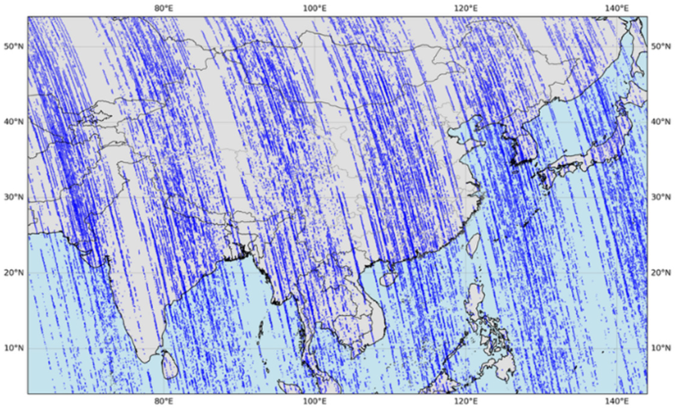
Figure 1 shows the study region and spatial distribution of the AGRI/CALIPSO matched samples during the study period from 1 January 2022 to 31 December 2022 (total 12 months). The study region extended from 2°N to 55°N and 60°E to 140°E, covering parts of East and South Asia with elevations ranging from 0 to 8 km, encompassing a variety of land-cover types including vegetation, water bodies, and bare soil [62]. The matched samples were distributed across most of the research area, and divided into training, validation, and test subsets. The data in February and August were selected to test the model performance, the remaining 10 months of data were used for model training. In the training process, two-thirds of the data were randomly sampled for training, while the remaining one-third was reserved for validation. As a whole, 279,636 matched samples were obtained, of which 150,734 samples were used for training, 75,347 for validation and 53,555 for testing, providing a robust foundation for model training and performance assessment.

2.2. Methodology

2.2.1. THMA Architecture

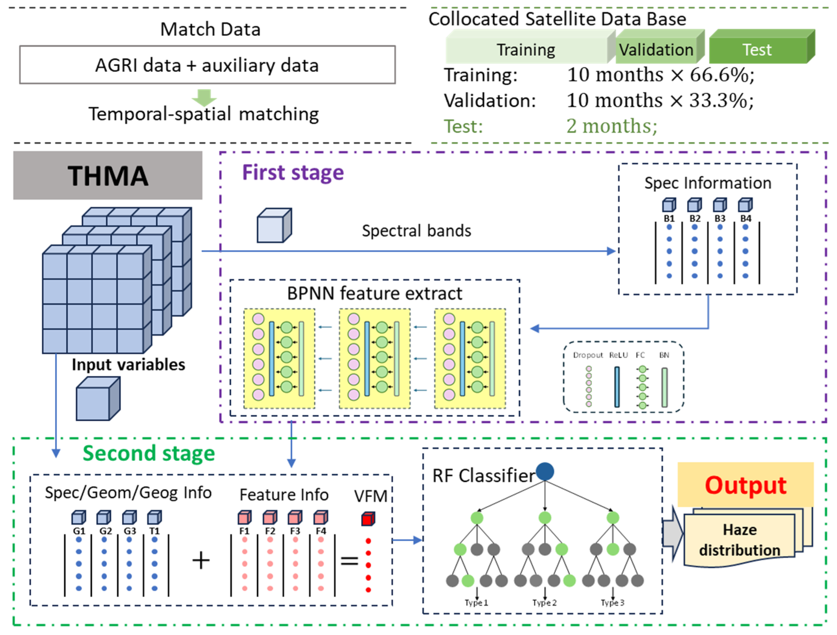
Based on the data sets constructed as described above, a two-stage model, named THMA, was developed for cloud, haze and clear air identification. This model employs a BPNN as the feature builder for nonlinear relationship learning and an RF as the strong classifier. The algorithm flowchart is shown in Figure 2.

As reported by Yan et al. [63], a Bidirectional Recurrent Neural Network can effectively extract features to improve modeling results. Similarly, we use a BPNN designed for feature extraction to construct the THMA first-stage model, which consists of three fully connected hidden layers, containing 64, 32, and 16 neurons, respectively. Each hidden layer employs the rectified linear unit (ReLU) activation function. ReLU enhances the model’s capacity for nonlinear representation by outputting the input value directly if it is positive, and zero otherwise. During training, the model’s parameters are optimized via backpropagation, minimizing a cross-entropy loss function. The Adam optimizer is used for this purpose. Adam adapts the learning rate for each parameter by computing estimates of the first-order moment (the mean) and second-order moment (the uncentered variance) of the gradients, while applying bias correction to these estimates. Key hyperparameters for Adam are set as follows: a learning rate of 0.001, first-moment decay rate of 0.9, second-moment decay rate of 0.999, and a numerical stability term of 1e-8 to ensure stable gradient updates. To monitor the training process, the average loss and average gradient magnitude are computed after each epoch. This helps in assessing the convergence speed and training stability, aiding in the prevention of overfitting to local optima. Collectively, this network, comprising the input, hidden, and output layers, functions as a powerful feature extractor. The fundamental operation within each hidden-layer neuron involves an affine transformation of its inputs, followed by the application of the nonlinear ReLU activation. The iterative backpropagation of the cross-entropy loss continuously refines the model’s weights and biases, enabling the network to learn complex, hierarchical, and discriminative feature representations from the input data.

The second stage is an RF classifier which takes the multi-dimensional features extracted from the first stage, spectral information, combined metrics and geometric and geographical information, as its inputs. This ensemble comprises 200 decision trees to ensure sufficient diversity for variance reduction while maintaining computational efficiency. To mitigate overfitting, each tree is constrained to a maximum depth of 15. Further regularization is applied by requiring a minimum of 10 samples to split an internal node and at least 5 samples to form a leaf node, ensuring that splitting decisions are statistically robust and thereby improving generalization. The model employs standard RF randomization techniques: it utilizes bootstrap aggregating (bagging) to create training subsets by sampling with replacement, and at each node split, it randomly selects a subset of candidate features following the square-root rule. The optimal split is determined by maximizing the reduction in Gini impurity. A fixed random seed of 42 is used for all stochastic processes to ensure reproducibility. Collectively, these hyperparameter settings strike a balance between model complexity, predictive variance, and computational efficiency.

This two-stage model, driven by the top of atmosphere spectral information directly observed by satellites, some combined spectral metrics, and other geometric and geographic information, provides the identification of clear air, cloud, and haze areas.

2.2.2. Performance Metrics

To evaluate our classification results, a set of quantitative metrics is required. In traditional cloud detection algorithms, only two categories, clear and cloud, are included. Consequently, metrics such as false alarm rate (FAR), specificity, precision, miss rate, probability of detection and leakage rate (LR) are usually employed for evaluation [64,65]. In this study, we retained the definitions of FAR and LR used in other studies to represent the proportions of misclassified cloud and clear air pixels, respectively. More specifically, the FAR represents the situation where, in clear air or haze conditions, the THMA model reports the presence of clouds, while LR indicates that the THMA reports the category of clear air in clouds or haze conditions. However, in this study, we have renamed the FAR and LR for such situations as the misclassification rate (MCR) of cloud and clear air. Thus, we define MCR for cloud, clear air and haze condition as follows:

$$MC{R}_{cla}={\displaystyle \frac{ITHM{A}_{Clear} \& VF{M}_{Haze or Cloud}}{Total number of pixel in comparison}},$$

(1)

$$MC{R}_{cld}={\displaystyle \frac{ITHM{A}_{Cloud} \& VF{M}_{Clear or Haze}}{Total number of pixel in comparison}},$$

(2)

$$MC{R}_{haz}={\displaystyle \frac{ITHM{A}_{Haze} \& VF{M}_{CLear or Cloud}}{Total number of pixel in comparison}},$$

(3)

The total MCR is the sum of the three MCRs defined by Equations (1)–(3), where $ITHMA$, $haz$, $cld$ and $cla$ are the abbreviations for the indicator of the THMA, haze, cloud and clear air, respectively. $ITHM{A}_x$ represents the category x predicted by the THMA for a single pixel, where x can be haze, cloud or clear sky. $VF{M}_{y or z}$ represents the category y or z observed by $VFM$ of pixels, where y and z can be haze, cloud or clear sky, different from x. $ITHM{A}_x \& VF{M}_{y or z}$ represent those pixels for which the true category is y or z, while the predicted category of the THMA is x.

In addition to the MCR, confusion matrices, precision, recall and F1 score were used for the assessment of THMA performance.

In a confusion matrix, let $N$ denote the original (unnormalized) confusion matrix, where each element $N_{i,j}$ represents the number of samples belonging to the true class $i$ that are predicted as class $j$. The diagonal elements $N_{i,i}$ indicate correctly classified samples, while the off-diagonal elements reflect misclassifications between different classes. Based on the original confusion matrix, standard evaluation metrics, including precision, recall, and F1 score, are computed for each class.

For a given predicted class $j$, precision measures the proportion of correctly classified samples among all samples predicted as class $j$, and is defined as:

$$Precisio{n}_j={\displaystyle \frac{N_{j,j}}{{{\displaystyle \sum }}_i{N}_{i,j}}}\times 100\%,$$

(4)

For a given true class $i$, recall measures the proportion of correctly classified samples among all samples whose true class is $i$, and is defined as:

$$Recal{l}_i={\displaystyle \frac{N_{i,i}}{{{\displaystyle \sum }}_j{N}_{i,j}}}\times 100\%,$$

(5)

For each class $i$, the F1 score is computed by combining the precision and recall values corresponding to class $i$, where ${\mathrm{Precision}}_i$ denotes the precision obtained when class $i$ is treated as the predicted class. The F1 score is the harmonic mean of precision and recall and is defined as:

$$F1 scor{e}_i={\displaystyle \frac{2\times Precisio{n}_i\times Recal{l}_i}{Precisio{n}_i+Recal{l}_i}},$$

(6)

In addition to these quantitative metrics, a normalized confusion matrix is employed to provide the comprehensive class-wise classification performance. In this row-normalized confusion matrix, each element represents the percentage of samples from a given true class that are assigned to each predicted class, obtained by normalizing the confusion matrix by the total number of samples in each true class.

2.2.3. Ablation Experiment Design

To definitively attribute performance gains to the two-stage architecture and evaluate the contribution of each stage, we conduct an ablation study comparing three models:

• Baseline A (RF-only). An RF classifier trained directly on the original variables. This baseline assesses the gain attributable solely to the BPNN’s feature extraction.
• Baseline B (BPNN-only). A standalone neural network, with the same architecture as the first stage, but capped with a task-specific output layer, was trained end-to-end for classification. This baseline isolates the performance of a purely machine learning approach.
• Proposed Model (BPNN + RF). The full two-stage THMA model, where the RF classifier is trained on the multi-dimensional features learned by the BPNN.

All models were trained and optimized on the same training and validation data sets, and their performances were compared using the metrics defined in Section 2.2.2. A statistically significant superiority of the proposed model over both baselines would validate the synergy of the two-stage design. This structured evaluation provides a holistic view of the model’s effectiveness, robustness, and the unique value of its hierarchical feature-learning and classification pipeline.

3. Results

3.1. Feature Screening

To optimize the input features in the second stage, we employ a recursive screening method based on the feature importance of the RF model [66]. In particular, the feature with the lowest current mean decrease impurity (MDI) score is removed, and the model is retrained. This process is repeated until the model performance shows a significant decline, at which point the feature set is considered the final optimal selection. The model performance is evaluated using Equations (1)–(3). Based on this procedure, the features listed in

Table 2. Input parameters used by THMA at the first and second stage.

	Variables in the First Stage	Variables in the Second Stage
Spectral information	CH1(0.47 µm), CH2(0.65 µm), CH3(0.825 µm), CH4(1.375 µm), CH5(1.61 µm), CH6(2.25 µm), CH8(3.75 µm), CH9(6.25 µm), CH10(7.1 µm), CH11(8.5 µm), CH12(10.7 µm), CH13(12.0 µm), CH14(13.5 µm)
Combined metrics	CH3/CH2, CH3/CH5, CH10-CH12, CH12-CH8, CH12-CH13, NDVI, NDSI, NDVI-SWIR	CH3/CH5, CH10-CH12, CH12-CH8, NDVI, NDSI
Geometric and geographic information	/	SZA, Elevation, Latitude, Longitude
Extracted features	/	N1, N5, N6, N7, N8, N10, N11, N12, N14 1

¹ N1, N2, … N16 are these features extracted from first stages and are partly used in second stage.

were selected as the inputs. The inputs in the second stage were top of atmosphere (TOA) reflectance in 13 spectral bands, NDVI, NDSI and NDVI-SWIR, 4 geometric and geographic variables and 9 features extracted from the first stage.

Through feature screening as described above, we identified several spectral channels and their combined metrics that are critical for haze mapping, based on their distinct physical interactions with atmospheric components. The TOA reflectance in the CH1 band (0.47 µm) demonstrates high sensitivity to Mie scattering by aerosol particles. Under heavy pollution conditions, enhanced scattering by haze particles can substantially increase the reflectance in this band [67]. CH12 (10.7 µm) lies within an atmospheric transmission window, primarily sensing thermal radiation emitted from the Earth’ surface and cloud tops. CH8 (3.75 µm) captures both reflected solar and emitted thermal radiation during daytime, making it effective for detecting low-altitude liquid clouds, ice clouds, and dust [12,68]. Furthermore, CH14 (13.5 µm) is effective for determining effective cloud cover and high-level clouds [68], while the combination of CH13 (12.0 µm) with other brightness temperatures (e.g., 10.7 µm) aids in distinguishing dense aerosol from cloud [69,70]. CH2 (0.65 µm) contributes by assisting in the identification of thick cloud [68]. For the combined metrics, CH3/CH5 can identify clouds over high-albedo deserts but is ineffective over dense forest canopy. CH10-CH12 shows some capability in detecting high- and mid-level clouds over land during early morning and late afternoon. CH12-CH8 is able to detect liquid-phase and ice-phase clouds in low-altitude regions. NDVI and NDSI can be used to distinguish forested land from snow/ice-covered surfaces. While the direct satellite observations and combined metrics described above have clear physical interpretations, other features extracted in the first stage of the THMA represent complex, non-linear transformations. Their specific physical meanings are not easily disentangled, though this does not diminish their potential importance within the model framework. All variables in Stage I contribute to the extracted features, the far-infrared bands exhibit a larger influence.

3.2. Model Accuracy Assessment

3.2.1. Ablation Experiment

To validate the cooperation performance and effectiveness of the two stages in the THMA model, we conducted an ablation experiment as described in Section 2.2.3. The results, i.e., the MCRs for cloud, haze and clear air for each month in the validation and test data sets, are presented in

Table 3. Model performance on the validation and test data set.

		Validation Data Set											Test Data Set
Model	Month	1	3	4	5	6	7	9	11	12	Ave	Total	2	8	Ave	Total
	$MC{R}_{cld}$ (%)	1.87	2.15	2.54	3.58	3.06	2.15	1.72	1.53	1.32	2.24	7.88	2.16	2.45	2.28	13.16
THMA	$MC{R}_{haz}$ (%)	3.02	2.30	3.07	3.63	2.90	2.59	3.71	2.49	2.94	2.96		4.41	7.98	5.83
	$MC{R}_{cla}$ (%)	1.97	2.06	2.56	3.40	2.91	3.06	3.07	3.38	1.40	2.68		5.38	4.56	5.06
	$MC{R}_{cld}$ (%)	1.78	2.62	3.08	3.99	3.77	2.85	1.82	1.53	0.99	2.55	9.97	3.26	2.57	2.99	16.11
RF	$MC{R}_{haz}$ (%)	3.70	2.68	4.28	4.63	4.20	5.02	5.82	3.61	3.37	4.18		4.10	12.09	7.27
	$MC{R}_{cla}$ (%)	3.30	2.91	3.13	3.80	3.67	2.86	3.30	3.79	2.07	3.23		6.89	4.29	5.86
	$MC{R}_{cld}$ (%)	1.47	1.21	1.27	2.17	2.20	2.27	2.33	1.72	1.72	1.79	12.96	1.07	2.34	1.57	14.64
BPNN	$MC{R}_{haz}$ (%)	5.30	5.63	8.78	7.70	6.06	5.45	6.42	6.95	3.59	6.39		6.80	5.04	6.10
	$MC{R}_{cla}$ (%)	4.36	3.61	4.79	5.80	5.58	4.65	6.46	3.61	3.59	4.76		5.01	9.96	6.97
	Sample Num	9053	9271	11,082	7972	7184	8805	9082	7831	5067	/	75,347	32,319	21,236	/	53,555

. The metrics in Table 3 show the good performance of the THMA model for the classification of clouds, haze and clear air, with MCRs averaged over the whole validation data of 2.24%, 2.96%, and 2.68%, respectively. The differences between the $MC{R}_{cld}$, $MC{R}_{haz}$ and $MC{R}_{cla}$, averaged over the whole validation data set of the THMA model are much smaller than those of the RF and BPNN baseline models. The total MCR for the THMA model of 7.88% is substantially smaller than for the RF (9.97%) and for BPNN (12.96%) models, showing the better overall performance of the THMA model. From a monthly perspective, the $MC{R}_{cld}$ of the THMA model varies between 1.32% and 3.58%, which is larger than for the BPNN model with 1.21% to 2.33% and smaller than for the RF model with 0.99% to 3.99%. For haze, the $MC{R}_{haz}$ varies between 2.30% and 3.71% for the THMA model, which is considerably smaller than for the RF model with 2.68% to 5.82% and for the BPNN model with 3.59% to 8.78%. Similarly, the $MC{R}_{cla}$ for the THMA model ranges from 1.40% to 3.40%, which is larger than for the RF model with 2.07% to 3.80%, and smaller than for the BPNN model with 3.59% to 6.46%.

As mentioned in Section 2.1.4, the data in February and August were set aside as test data to assess the generalization capability and stability of the model through the comparison with the accuracy of the validation data set. The performance of the THMA model for these two test months is consistently better than that of the baseline models. Specifically, for the THMA model the $MC{R}_{cld}$, $MC{R}_{haz}$ and $MC{R}_{cla}$ averaged over the whole test data set are 2.28%, 5.83% and 5.06%, respectively. Most of the three MCR metrics for the RF and BPNN models are larger than for the THMA model, except for the $MC{R}_{cld}$ for the BPNN model. In addition, the differences between the $MC{R}_{cld}$, $MC{R}_{haz}$ and $MC{R}_{cla}$ over the whole test data set are smallest for the THMA model. The MCRs for the test data set are slightly higher than for the validation data set, by 0.04%, 2.87% and 2.38% for the $MC{R}_{cld}$, $MC{R}_{haz}$ and $MC{R}_{cla}$ respectively. For comparison, the $MC{R}_{haz}$ for the RF and BPNN models are 7.27% and 6.10%, respectively, while their $MC{R}_{cla}$ are 5.86% and 6.97%. These data show that for both the BPNN and RF models the $MC{R}_{haz}$ and $MC{R}_{cla}$ are higher than for the THMA model applied to the test data set.

3.2.2. Statistical Evaluation of the THMA Model

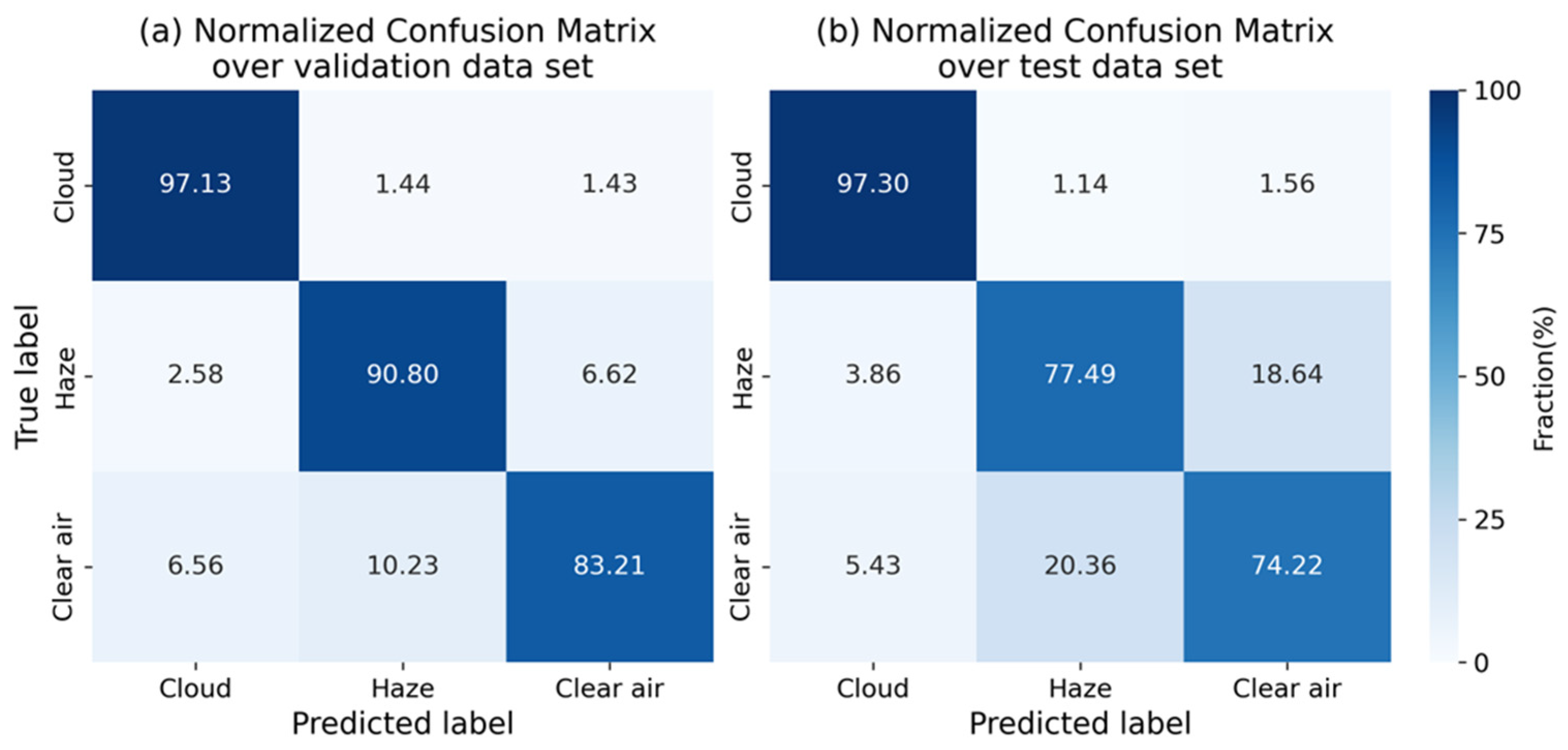
The precision, recall and F1 score in

Table 4. Precision, recall and F1 scores of the THMA model for the validation and test data sets.

	Metrics over Validation Data Set				Metrics over Test Data Set
	Precision %	Recall %	F1 Score	Num 1	Precision %	Recall %	F1 Score	Num 1
Cloud	95.38	97.13	0.96	35,852	95.65	97.30	0.96	27,556
Haze	90.24	90.80	0.91	22,724	75.21	77.49	0.76	12,215
Clear air	87.37	83.21	0.85	16,771	79.07	74.22	0.77	13,784

¹ Number of samples.

show the good performance of the THMA model for both the validation and test data sets, with differences across clouds, haze and clear air. Using the validation data set, the performance of THMA is highly reliable for cloud identification with a precision of 95.38%, a recall of 97.13%, and an F1 score of 0.96. For haze, the precision and recall values are 90.24% and 90.80%, respectively, resulting in an F1 score of 0.91. For clear air the THMA performance is lowest of the three conditions but still very good with a recall of 83.21%, a precision of 87.37% and an F1 score of 0.85. These metrics suggest a higher false negative rate for clear air conditions than for haze or clouds.

Using the test data set, a similar performance is observed with a slight decrease in accuracy, particularly for haze and clear air. For cloud identification, the precision is 95.65%, recall is 97.30%, and the F1 score is 0.96. Thes metrics are comparable to those for the validation data set. In contrast, for haze identification the evaluation using the test data set results in lower performance than for the validation data set, with precision of 75.21% and recall of 77.49%, resulting in an F1 score of 0.76. For clear air identification the metrics are similar to those for haze and smaller for the test data set than for the validation data set.

The normalized confusion matrices for the identification results for the validation and test data sets are presented in Figure 3. For haze samples, a substantial proportion is misclassified as cloud or clear air, which directly contributes to the reduction in recall from 90.80% on the validation data set to 77.49% on the test data set. Similarly, clear air samples are frequently confused with haze, resulting in a recall drop from 83.21% to 74.22%. In contrast, for clouds the recall of 97% for both data sets indicates the good performance of THMA for cloud identification.

3.3. Application of THMA in Two Case Studies

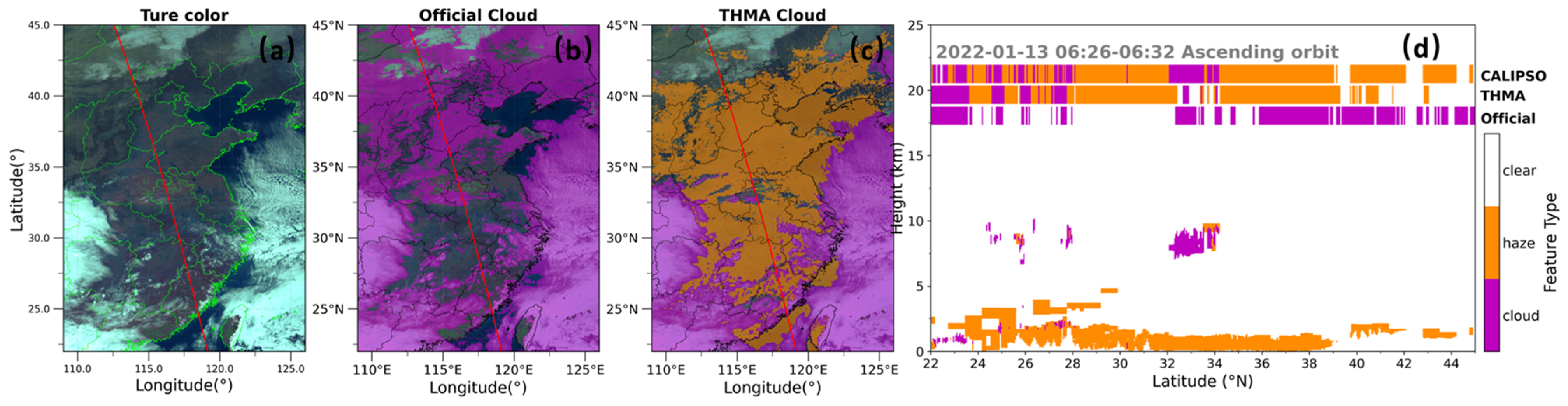
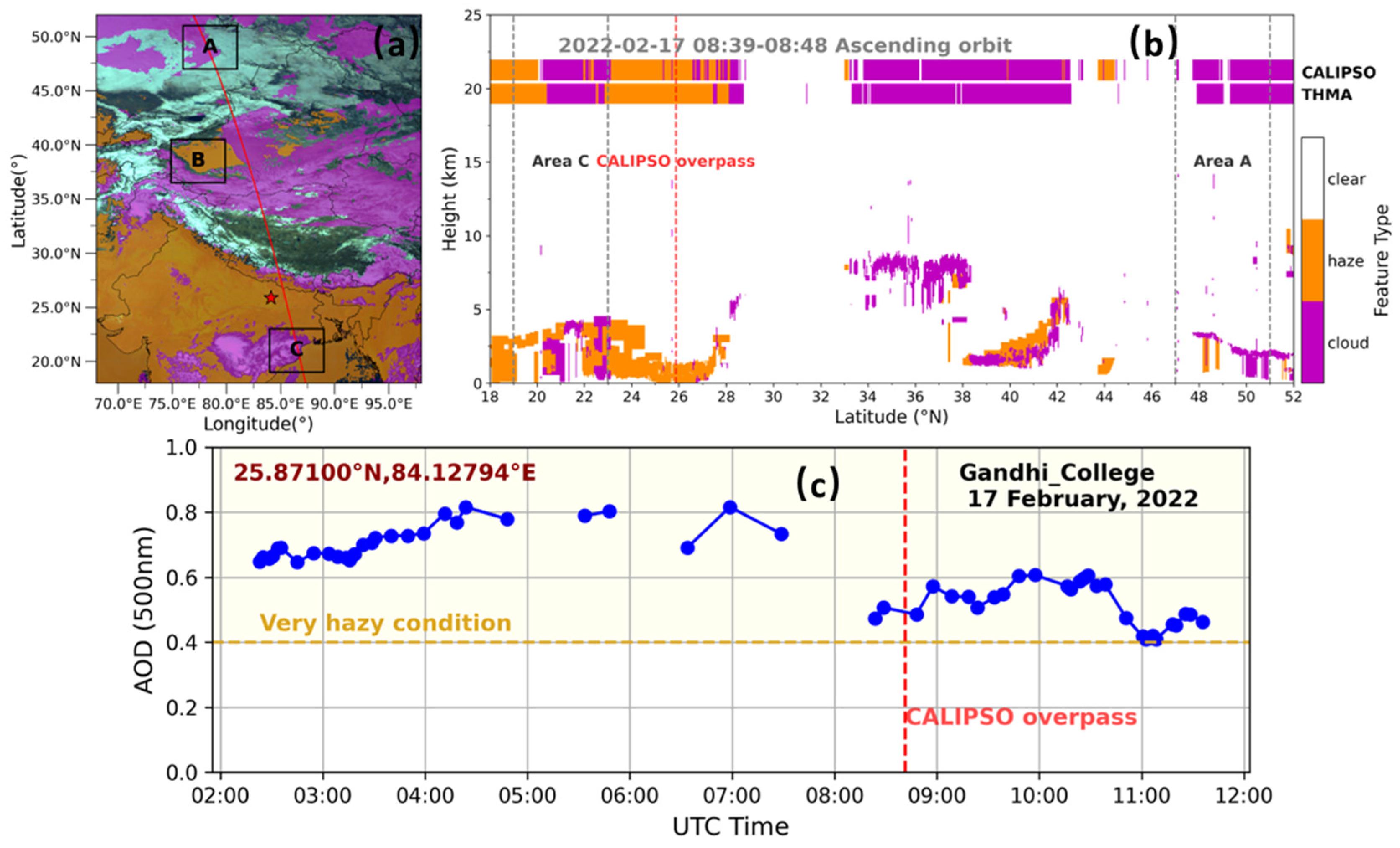
To evaluate the capability of the THMA model in identifying detailed features within AGRI cloud imagery, two representative cases were selected for in-depth analysis. Case I pertains to a severe haze event that occurred in northeastern China in January 2022, impacting areas including southern Hebei, northern Henan, and western Shandong (https://www.cma.gov.cn/zfxxgk/gknr/qxbg/202307/t20230707_5633816.html; accessed on 18 January 2026). A single day (13 January 2022) was chosen for analysis within the region bounded by 110°E–125°E and 22°N–45°N (Figure 4). Case II corresponds to an event on 17 February 2022, analyzed over the area extending from 68°E–95°E and 18°N–52°N (Figure 5). Both cases were selected to coincide with CALIPSO overpasses, ensuring the availability of vertical profile data from the CALIPSO track for validation.

3.3.1. Case I

Figure 4 presents results from the application of the THMA model to AGRI data over northeastern China on 13 January 2022 at 06:15 UTC, with comparisons to the official AGRI cloud mask and the coincident CALIPSO VFM product. The CALIPSO trajectory is indicated by the red line. The official AGRI cloud mask (Figure 4b) shows that the cloud area as identified in this product covers a large part of the study area, with about 1/3 of the area cloud-free, i.e., the dark areas over eastern Hubei, northern Jiangxi, central Anhui, and eastern Jiangsu, as well as some smaller areas in the north of the study area (indicated in dark green and light blue). However, the cloud areas determined by the THMA model are much smaller, and to a large extent confined to the areas which are showing cloud in the true color image (Figure 4c), while the feature over most of the remaining areas is determined to be haze (the orange color).

The CALIOP vertical cross-section in Figure 4d shows a haze layer adjacent to the surface extending over heights of 1–2 km along most of the track between 28°N and 39°N, or above the surface extending over up to 4km at lower latitudes and thin haze layers at about 2 km above the surface north of 40°N. Figure 4d also shows the occurrence of clouds and haze between 7.5 and 10 km. Comparison of the cloud and haze features derived from THMA and CALIOP shows reasonable agreement overall, but with discrepancies south of 28°N and between 32°N and 34°N. At higher latitudes discrepancies are observed between the haze and clear air classification. THMA incorrectly identifies part of the haze layer near 23°N as cloud, and high-altitude clouds near 7.5 km between 32°N and 34.5°N are in part misclassified as clear air or haze. This misclassification of cloud near 7.5 km between 32°N and 34.5°N may be related to the inherent physical properties of high-altitude clouds. Such clouds typically exhibit low optical thickness, resulting in less sensitivity in the visible and infrared bands [68,71]. Moreover, high clouds are mainly composed of ice crystals with complex shapes and variable particle size distributions, leading to pronounced differences in scattering and absorption responses across spectral bands [72,73] and thereby increasing the uncertainty in cloud-type classification. In addition, over ice-covered bright surfaces between 40°N and 44°N, labeled by NDSI in Figure S1, THMA misclassifies haze as clear air (Figure 4d). The AGRI cloud-mask product successfully identifies most of the regions labeled as cloud by THMA. Haze-dominated areas north of 34°N are identified as cloud in the AGRI official product, while also over ice-covered surfaces between 42°N and 45°N, the official product identifies clear air as cloud. The results from this case study show that the determination of the occurrence of haze (with haze defined in Section 2.1.4) by the THMA is in reasonable agreement with CALIPSO VFM results, with 19.05% misclassifications as clear air and 7.00% as cloud. Comparison of the spatial distributions of the AGRI official cloud product and the THMA haze distribution shows that a large proportion of haze is misclassified by the official cloud product.

3.3.2. Case II

Case II shows the application of THMA over a large area including regions in north India, the northwest deserts of China, and the northern snow-covered areas of east Kazakhstan. The distribution of haze and clouds over this area, as determined by application of THMA to AGRI data on 17 February 2022 at 09:00 UTC is presented in Figure 5a. Figure 5b shows the vertical distributions of the cloud, haze and clear air features as deduced form the CALIPSO VFM along the trajectory, with the dominant feature plotted in the horizontal bar at the top. The cloud and haze predicted by THMA along the CALIPSO trajectory are indicated in the second horizontal bar. Figure 5c shows the AOD time series on 17 February 2022 from the Gandhi College AERONET site (25.87°N, 84.31°E). The closest horizontal distance between the Gandhi College site and the CALIOP trajectory (nadir) is 128.53 km (Figure 5a). Figure 5c shows that the AOD at this site was larger than 0.4 which indicates the occurrence of haze [59] and confirms the haze identification by both the THMA (Figure 5a) and the CALIPSO VFM (Figure 5b).

Comparison of the features in Figure 5b shows that the THMA successfully identified haze between 18°N and 20°N and 23.2°N and 27.5°N, as well as the clear sky regions between 29°N and 33°N, 42.5°N and 43.5°N, and 44.5°N and 47.5°N, with only a few cloud/haze misclassifications. A small clear air area was identified as a CALIPSO feature between 20°N and 20.2°N, but not by the THMA. A haze layer extending from close to the surface to heights of approximately 4 km is present between 23°N and 24.5°N, and THMA successfully detected this feature. At latitudes between 24.5°N and 27.5°N, near-surface haze reached up to about 1.5 km, with some sporadic clouds not identified by the THMA, which only shows haze in this area.

In the regions between 20°N and 23.2°N, and between 38°N and 42.5°N, CALIOP observations indicate vertically overlapping clouds and haze, which pose challenges for haze identification by the THMA. In these cases, the cloud features dominate, following the identification scheme explained in the caption of Figure 4, and THMA is only able to identify the presence of haze for a few instances at latitudes between 22°N and 23°N. At latitudes between 26.5°N–28.5°N, only few clouds are observed in the CALIOP data and both the THMA and the CALIPSO VFM identified haze, albeit with some misclassification by THMA.

3.4. Diurnal Variation of Cloud and Haze

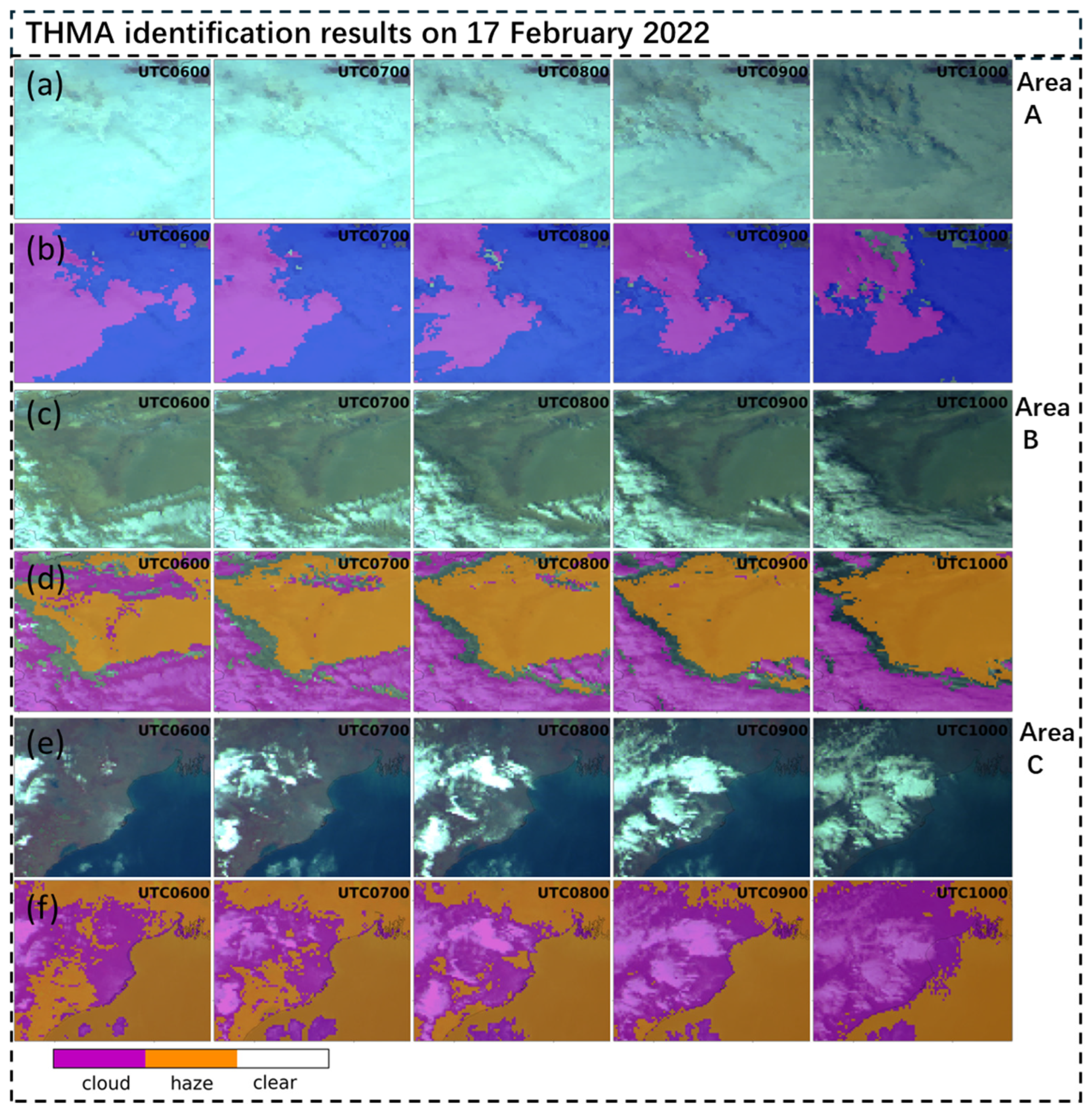
Figure 6 shows the THMA-derived variation of clouds and haze over three areas, indicated in Figure 5 by A, B and C, from 06:00 to 10:00 UTC on 17 February 2022. For each area, two rows of images are presented, with the top row, indicated by (a, c, d), showing true color images and the second row (b, d, e) indicating the THMA-derived cloud, haze and clear air areas indicated with the same color scheme as in Figure 4 and Figure 5. Figure 6a,b shows the results for area A. Area A includes the north of Xinjiang autonomous region in the northwest of China, and neighboring countries. The winters are very cold and the surface is frozen. The NDSI map in Figure S2 shows that the surface was covered with ice. The true color images of the area show that it is difficult to distinct between the ice-covered surface and overlying clouds. The color changes as time progresses (note that the area is located about 3 hours west of Beijing, i.e., local solar time is about UTC + 5) and the scattering angle changes with SZA. The THMA-derived maps show the temporal evolution of the identified features, only cloud (purple) and clear air, overlaid on a base map with NDSI > 0.36, which renders clear air blue. At 06:00 UTC, clouds extend over the western part of area A, narrowing toward the east in a triangular shape where clouds occur only in the middle. In the next few hours, cloud cover in the eastern and southwestern regions shrinks and eventually vanishes, leaving clear air over the underlying ice surface, while in the northwest the cloud area expands eastward between 06:00 and 09:00 UTC, increasingly obscuring the surface until partial dissipation at 10:00 UTC. The comparison between the THMA results and the CALIPSO VFM in Figure 5, at 09:00 UTC, shows that THMA correctly classified cloud and clear air along the CALIPSO track in Area A.

Figure 6c,d focus on an area including the Taklamakan Desert and surrounding mountains. The true color images in row (c) clearly show the occurrence of cloud over the mountain areas in the south, west and, to a lesser extent, in the north. The colors change with increasing SZA which may also influence the cloud identification, while in some areas, such as in the southeast and in the north of the image, the cloud cover clearly evolves. The clouds are well-reproduced by the THMA (row (d)), which also clearly reproduces the haze over the Taklamakan Desert. Furthermore, clear air is identified between the haze and cloud areas. The reason for the occurrence of clear air may be mountains preventing transport, but the investigation of this phenomenon is beyond the scope of the current study. The THMA successfully identifies most visually apparent cloud features, missing only a small number of isolated cloud pixels. Although the southwestern cloud system appears discontinuous in the true-color image, THMA depicts it as a quasi-continuous structure. This indicates that in mixed cloud–haze regions, THMA tends to classify ambiguous or partially cloud-contaminated pixels as cloud, which is consistent with the analysis in Section 3.3.

Figure 6e,f, focus on an area in the northeast of India, including part of the Gulf of Bengal (most of the blue area in row (e)). The true color images in row (e) show that virtually the whole land area was covered by a cloud system that evolved between 06:00 and 10:00 UTC. During this period, the color changed and, visually, the cloud system seems to become smaller. Some smaller clouds are observed in the south of the images, over the ocean. The shading to the southeast of the large cloud system, extending over the ocean, indicates the occurrence of haze. The latter is confirmed by the THMA results in row (f). However, the THMA results also show that the northern part of the visually apparent cloud system is actually haze, while to the south a large haze area is also identified, which during the observation period evolved into cloud. In contrast to the visual observation in row (e), the THMA results indicate an increase of the cloud-covered area, in particular toward the north, and much of the haze evolves into cloud. In the image at 10:00 UTC, all land area is cloud-covered, except for an area in the northeast. Also the smaller clouds in the south of area C, over the ocean, have merged into a larger cloud. The THMA results show that haze occurred over most of the ocean, whereas cloud occurred over most of the land area. The latter is confirmed by the comparison between the THMA results and the CALIPSO VFM (case II, Figure 5).

3.5. Number of Haze Days

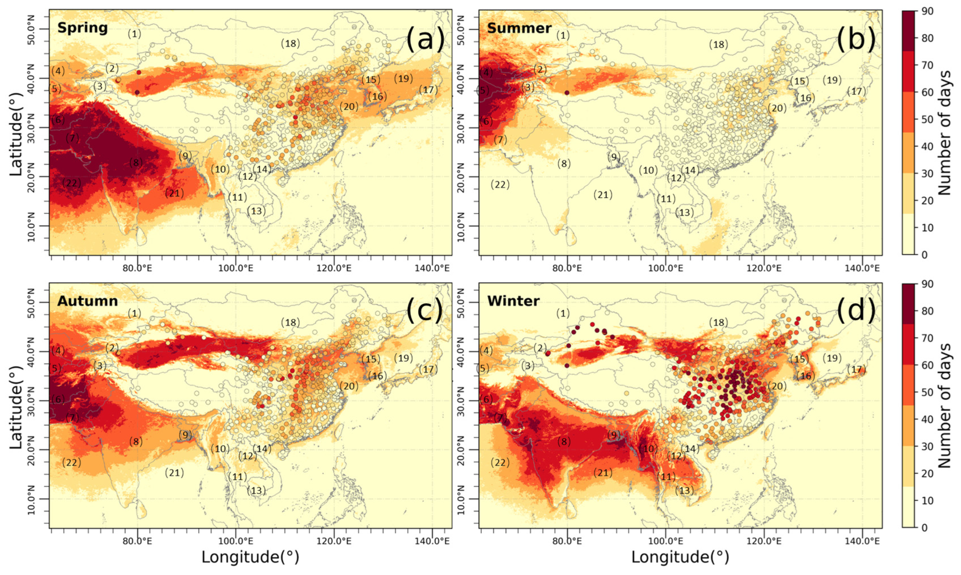
The spatial pattern and seasonal variations of the number of haze days (defined as a day when haze occurs) were studied over an area between about 62°E–144°E, 4°N–54°N, encompassing South and East Asia. The results were compared with city-averaged ground-based observations of PM_2.5, exceeding 35 μg/m³. The results are presented in Figure 7 which shows the spatial distributions of the number of haze days during spring, summer, autumn and winter. The data in Figure 7 show the strong spatiotemporal variation of the number of haze days, with the highest number in the western part of the study area in the spring, summer and autumn, whereas during the winter the highest concentrations are observed over India and China. High numbers of haze days occur over the Taklamakan Desert all year round, but with strong seasonal variation. Although the highest dust storm activity occurs in the spring, apparently the aerosol mass concentration levels are also high in other seasons.

While the seasonal variation of haze is most pronounced over monsoonal Asia, the aerosol concentrations over the vast arid interior of Central and West Asia are high throughout the year, predominantly driven by dust [41,74,75]. Satellite observations indicate that core dust source regions, including southern Afghanistan, Pakistan, and the border areas of Uzbekistan, Turkmenistan, and southern Kazakhstan, experienced more than 75 haze days in 2022, and a similar number of haze days occurred during the summer over western and eastern Uzbekistan, and over eastern Turkmenistan. The haze occurring in these areas is different from the anthropogenic haze in highly populated and industrialized areas such as in eastern China. However, due to the sparse ground-based observations in these areas, the study of haze in these regions relies mostly on satellite and re-analysis data [76,77,78,79]. The THMA, by leveraging the temporal and spatial variations presented by satellites, offers potential for the study of the temporal and spatial evolution of haze in these regions.

Based on the satellite observations in 2022, the core severe haze regions within China, primarily driven by anthropogenic emissions, are concentrated in the densely populated areas including the North China Plain, central China and the Sichuan Basin and in desert areas including the Taklamakan (discussed above) and Gobi Deserts and downwind areas influenced by dust transport. The number of haze days in these areas shows a pronounced seasonal variation tied to meteorological conditions, with the lowest number during the summer monsoon (often smaller than 15 days), a larger number of days in the spring (reaching 30–45 days), and peaks in the stagnant autumn and winter seasons. The numbers of haze days are up to 45–60 days in autumn and up to 45–75 days in winter in the most affected parts of these regions.

Over northern India and the Indo-Gangetic Plain, the number of haze day also shows significant seasonal variation, influenced by both local anthropogenic emissions and natural dust transported from upstream arid regions. The number of haze days exceeds 75 days in the core regions during spring and winter, decreases during the summer monsoon, and grows again to 30–75 days in autumn. This pattern reflects combined effects of pollution and dust influences.

Furthermore, an increase in haze days is observed in parts of Southeast Asia during autumn and winter. In Japan, higher numbers of haze days (45–60 days) are notably confined to the eastern coastal regions in winter, while a springtime increase may be attributed in part to the long-range transport of natural dust from the Asian continent. It is noted that the numbers reported above refer to the study year (2022) and may vary between years.

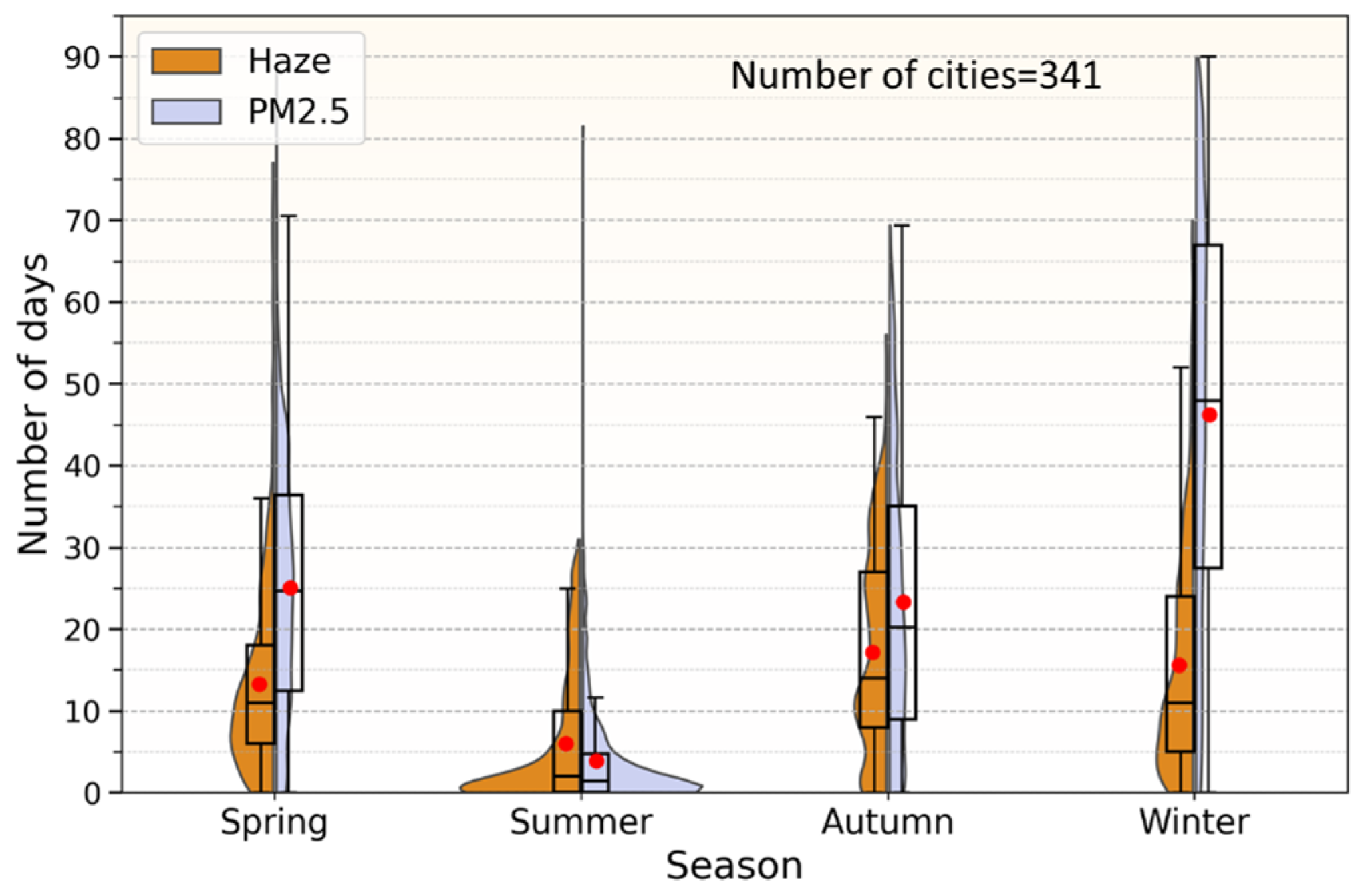
In addition to the THMA-derived number of haze days, PM_2.5-based haze days, derived for major cities in China, are presented in Figure 7. Comparison of the THMA-based and PM_2.5-based number of haze days shows a systematic discrepancy with ground-based stations reporting a higher value. To quantify this difference, Figure 8 and Table S1 provide a statistical comparison of the number of haze days derived from satellite and ground-based measurements for the four different seasons. The data in Table S1 show that in spring, satellite and ground-based estimates average 13.1 and 25.1 days, respectively; in summer, 6.0 versus 3.9 days; and in autumn, 16.9 versus 23.3 days. The most substantial difference occurs in winter, with satellite observations averaging only 15.3 haze days as compared to 46.2 days from ground-based observations. Over the whole year 2022, this results in a total of 51.2 satellite-derived haze days, markedly less than the ground-based total of 98.5 days. From the perspective of data distribution, the violin plots in Figure 8 show that the interquartile range for ground-based observations is substantially larger than that for satellite data in winter, spring, and autumn, indicating greater variability in surface observations. This difference is minimal only in summer. The elongated upper tails of the violin distributions for the PM_2.5 observations, and their absence in the THMA results, confirm the larger number of haze days derived from ground-based observations.

The discrepancy between the numbers of haze days derived from ground-based and satellite observations may be due to both the haze day definitions used and the observation strategy. In the current study, a ground-based haze day is defined using a PM_2.5 > 35 μg/m³ threshold. As a result, the number of haze days identified from ground-based observations is substantially higher than that derived from satellite observations, particularly during autumn and winter. Adopting a higher PM_2.5 concentration threshold in future analyses, such as >55.5 or >75 μg/m³, may improve consistency between satellite-derived and ground-based haze metrics. The observation strategy may be another major factor explaining the systemic underestimation of cloud cover, which obstructs satellite observations. As documented in Figure S3 and the accompanying data, satellite observations are obscured by clouds for an average of 63.6 days per year. This limitation is particularly acute in central and southeastern China, because these regions coincidentally host a high density of ground-based monitoring sites. Consequently, while ground-based measurements in these areas frequently record haze, concurrent cloud cover often prevents its detection from space. In contrast, the cloud-free conditions prevalent in northwestern China allow for more effective satellite monitoring, aligning results more closely with ground truth in those arid regions. Thus, while the satellite approach significantly expands spatial coverage for haze monitoring, especially in data-sparse regions, its efficacy is inherently constrained by cloud interference. This analysis underscores the complementary of satellite and ground-based networks, with the former providing essential broad-scale spatial context and the latter delivering accurate local measurements for all weather conditions.

4. Conclusions

Due to rapid industrial and social development, anthropogenic emissions have led to an increase in air pollution and the associated number of haze days in developing countries, particularly in regions such as eastern and central China and India. Concurrently, climate change has increased the occurrence of extreme weather events, altering the number of haze days caused by dust aerosol. Conventionally, haze monitoring typically relies on ground-based observations, which are limited in spatial coverage and representativeness. Satellite observations, especially from geostationary platforms, offer a valuable alternative by providing continuous, wide-area coverage. In this study, we propose a two-stage model, named THMA, for application to geostationary observations from the FY-4 AGRI sensor. The model first extracts haze-sensitive features using a BPNN, and then performs haze identification based on an RF method. We demonstrate that applying this model to multi-channel FY-4A AGRI observations yields the spatial distribution of haze, clouds, and clear air over Asia in 2022.

The results indicate that THMA effectively mitigates the confusion between haze and clouds inherent in traditional aerosol retrieval algorithms and significantly reduces the misclassification of high aerosol concentrations as cloud. Ablation experiments confirm that the model performs better on both validation and test data sets than the individual baseline models, with misclassification rates for clouds, haze, and clear air of 2.24%, 2.96%, and 2.68% on the validation set, and 2.28%, 5.83%, and 5.06% on the test set, respectively. This indicates that THMA shows good performance on both the validation and test data sets, demonstrating good stability. A detailed comparison with CALIOP observations further shows that THMA performs satisfactorily in classifying clouds, haze, and clear air across most regions, thereby successfully extending the conventional binary cloud-clear classification into a three-category task. Also, the model retains good classification capability in vertically overlapping regions of clouds and haze. However, misclassification occurs occasionally even over bright surfaces such as deserts or ice/snow, and near cloud edges, small haze patches, and broken cloud fields, as discussed in Section 3.3 and observed, for example, in Figure 4b.

Based on observations in 2022, we further analyzed the number of haze days in China. The annual average number of haze days across China was 51.3 days. Haze days over the North China Plain, central China, and the Sichuan Basin ranged in 2022 from 45–60 in autumn and 45–75 in winter, likely due to intensive anthropogenic emissions and frequent stagnant weather conditions in these seasons. In contrast, the number of haze days over the Taklamakan region exceeded 75 in the autumn, which was clearly driven by natural dust. Similarly, high numbers of haze days (over 75) were observed in regions dominated by natural sources, such as Central Asia, Pakistan, and southern Afghanistan. In northern India, where both dust and anthropogenic emissions contribute, haze days reached 45–75 during autumn and winter. The THMA model effectively captures haze distribution and is applicable to large-scale atmospheric monitoring.

This study confirms the capability of the THMA model to identify haze resulting from both anthropogenic and natural emissions, and underscores the importance of large-scale satellite-based haze mapping for aerosol research. Nevertheless, although satellite monitoring offers extensive spatial coverage, it is susceptible to cloud obstruction, which can significantly reduce the detection capability of near-surface haze and lead to lower haze frequency estimates compared to ground-based measurements. This further highlights the complementary value of satellite remote sensing and ground-station observations, and their integration will greatly advance haze analysis and mapping capabilities.

References

1. World Meteorological Organization (WMO). Haze. In International Cloud Atlas; World Meteorological Organization: Geneva, Switzerland; Available online: https://cloudatlas.wmo.int/en/haze.html (accessed on 18 January 2026).
2. Sun, Y.; Chen, C.; Zhang, Y.; Xu, W.; Zhou, L.; Cheng, X.; Zheng, H.; Ji, D.; Li, J.; Tang, X.; et al. Rapid Formation and Evolution of an Extreme Haze Episode in Northern China during Winter 2015. Sci. Rep. 2016, 6, 27151. [Google Scholar] [CrossRef] [Scilit]
3. Neff, J.C.; Reynolds, R.L.; Munson, S.M.; Fernandez, D.; Belnap, J. The Role of Dust Storms in Total Atmospheric Particle Concentrations at Two Sites in the Western U.S. J. Geophys. Res. Atmos. 2013, 118, 11201–11212. [Google Scholar] [CrossRef] [Scilit]
4. Vasilakopoulou, C.N.; Matrali, A.; Skyllakou, K.; Georgopoulou, M.; Aktypis, A.; Florou, K.; Kaltsonoudis, C.; Siouti, E.; Kostenidou, E.; Błaziak, A.; et al. Rapid Transformation of Wildfire Emissions to Harmful Background Aerosol. npj Clim. Atmos. Sci. 2023, 6, 218. [Google Scholar] [CrossRef] [Scilit]
5. Bates, J.T.; Fang, T.; Verma, V.; Zeng, L.; Weber, R.J.; Tolbert, P.E.; Abrams, J.Y.; Sarnat, S.E.; Klein, M.; Mulholland, J.A.; et al. Review of Acellular Assays of Ambient Particulate Matter Oxidative Potential: Methods and Relationships with Composition, Sources, and Health Effects. Environ. Sci. Technol. 2019, 53, 4003–4019. [Google Scholar] [CrossRef] [Scilit] [PubMed]
6. Johnston, F.H.; Henderson, S.B.; Chen, Y.; Randerson, J.T.; Marlier, M.; DeFries, R.S.; Kinney, P.; Bowman, D.M.J.S.; Brauer, M. Estimated Global Mortality Attributable to Smoke from Landscape Fires. Environ. Health Perspect. 2012, 120, 695–701. [Google Scholar] [CrossRef] [Scilit]
7. Yu, W.; Xu, R.; Ye, T.; Abramson, M.J.; Morawska, L.; Jalaludin, B.; Johnston, F.H.; Henderson, S.B.; Knibbs, L.D.; Morgan, G.G.; et al. Estimates of Global Mortality Burden Associated with Short-Term Exposure to Fine Particulate Matter (PM2·5). Lancet Planet. Health 2024, 8, e146–e155. [Google Scholar] [CrossRef] [Scilit]
8. Das, S.K.; Chatterjee, A.; Ghosh, S.K.; Raha, S. An Integrated Campaign for Investigation of Winter-Time Continental Haze over Indo-Gangetic Basin and Its Radiative Effects. Sci. Total Environ. 2015, 533, 370–382. [Google Scholar] [CrossRef] [Scilit]
9. Ehn, M.; Thornton, J.A.; Kleist, E.; Sipilä, M.; Junninen, H.; Pullinen, I.; Springer, M.; Rubach, F.; Tillmann, R.; Lee, B.; et al. A Large Source of Low-Volatility Secondary Organic Aerosol. Nature 2014, 506, 476–479. [Google Scholar] [CrossRef] [Scilit]
10. Bikkina, S.; Andersson, A.; Kirillova, E.N.; Holmstrand, H.; Tiwari, S.; Srivastava, A.K.; Bisht, D.S.; Gustafsson, Ö. Air Quality in Megacity Delhi Affected by Countryside Biomass Burning. Nat. Sustain. 2019, 2, 200–205. [Google Scholar] [CrossRef] [Scilit]
11. Lu, S.; Gong, S.; He, J. Uncertainty Analysis of Spatiotemporal Characteristics of Haze Pollution from 1961 to 2017 in China. Atmos. Pollut. Res. 2020, 11, 310–318. [Google Scholar] [CrossRef] [Scilit]
12. Shang, H.; Chen, L.; Letu, H.; Zhao, M.; Li, S.; Bao, S. Development of a Daytime Cloud and Haze Detection Algorithm for Himawari-8 Satellite Measurements over Central and Eastern China. J. Geophys. Res. Atmos. 2017, 122, 3528–3543. [Google Scholar] [CrossRef] [Scilit]
13. Booth, B.B.B.; Dunstone, N.J.; Halloran, P.R.; Andrews, T.; Bellouin, N. Aerosols Implicated as a Prime Driver of Twentieth-Century North Atlantic Climate Variability. Nature 2012, 484, 228–232. [Google Scholar] [CrossRef] [Scilit]
14. Kulmala, M.; Kontkanen, J.; Junninen, H.; Lehtipalo, K.; Manninen, H.E.; Nieminen, T.; Petäjä, T.; Sipilä, M.; Schobesberger, S.; Rantala, P.; et al. Direct Observations of Atmospheric Aerosol Nucleation. Science 2013, 339, 943–946. [Google Scholar] [CrossRef] [Scilit] [PubMed]
15. Li, J.; Han, Z.; Wu, Y.; Xiong, Z.; Xia, X.; Li, J.; Liang, L.; Zhang, R. Aerosol Radiative Effects and Feedbacks on Boundary Layer Meteorology and PM2.5 Chemical Components during Winter Haze Events over the Beijing-Tianjin-Hebei Region. Atmos. Chem. Phys. 2020, 20, 8659–8690. [Google Scholar] [CrossRef] [Scilit]
16. Zhan, J.; Chang, W.; Li, W.; Wang, Y.; Chen, L.; Yan, J. Impacts of Meteorological Conditions, Aerosol Radiative Feedbacks, and Emission Reduction Scenarios on the Coastal Haze Episodes in Southeastern China in December 2013. J. Appl. Meteorol. Climatol. 2017, 56, 1209–1229. [Google Scholar] [CrossRef] [Scilit]
17. Huang, L.; Jiang, J.H.; Tackett, J.L.; Su, H.; Fu, R. Seasonal and Diurnal Variations of Aerosol Extinction Profile and Type Distribution from CALIPSO 5-year Observations. J. Geophys. Res. Atmos. 2013, 118, 4572–4596. [Google Scholar] [CrossRef] [Scilit]
18. Robbins, D.; Poulsen, C.; Siems, S.; Proud, S. Improving Discrimination between Clouds and Optically Thick Aerosol Plumes in Geostationary Satellite Data. Atmos. Meas. Tech. 2022, 15, 3031–3051. [Google Scholar] [CrossRef] [Scilit]
19. Shang, H.; Chen, L.; Tao, J.; Su, L.; Jia, S. Synergetic Use of MODIS Cloud Parameters for Distinguishing High Aerosol Loadings From Clouds Over the North China Plain. IEEE J. Sel. Top. Appl. Earth Obs. Remote Sens. 2014, 7, 4879–4886. [Google Scholar] [CrossRef] [Scilit]
20. Tan, S.-C.; Zhang, X.; Wang, H.; Chen, B.; Shi, G.-Y.; Shi, C. Comparisons of Cloud Detection among Four Satellite Sensors on Severe Haze Days in Eastern China. Atmos. Ocean. Sci. Lett. 2018, 11, 86–93. [Google Scholar] [CrossRef] [Scilit]
21. Zhang, X.; Wang, H.; Che, H.-Z.; Tan, S.-C.; Shi, G.-Y.; Yao, X.-P. The Impact of Aerosol on MODIS Cloud Detection and Property Retrieval in Seriously Polluted East China. Sci. Total Environ. 2020, 711, 134634. [Google Scholar] [CrossRef] [Scilit]
22. Ackerman, S.; Strabala, K.; Menzel, P.; Frey, R.; Moeller, C.; Gumley, L.; Baum, B.; Seemann, S.W.; Zhang, H. Discriminating Clear-Sky from Cloud with MODIS: Algorithm Theoretical Basis Document (MOD35); MODIS Cloud Mask Team, NASA Goddard Space Flight Center: Greenbelt, MD, USA, 2006. Available online: https://modis-images.gsfc.nasa.gov/_docs/MOD35:MYD35_ATBD_C005.pdf (accessed on 21 January 2026).
23. Martins, J.V.; Tanré, D.; Remer, L.; Kaufman, Y.; Mattoo, S.; Levy, R. MODIS Cloud Screening for Remote Sensing of Aerosols over Oceans Using Spatial Variability. Geophys. Res. Lett. 2002, 29, 1619. [Google Scholar] [CrossRef] [Scilit]
24. Hutchison, K.D.; Iisager, B.D.; Kopp, T.J.; Jackson, J.M. Distinguishing Aerosols from Clouds in Global, Multispectral Satellite Data with Automated Cloud Classification Algorithms. J. Atmos. Ocean. Technol. 2008, 25, 501–518. [Google Scholar] [CrossRef] [Scilit]
25. Si, Y.; Chen, L.; Zheng, Z.; Yang, L.; Wang, F.; Xu, N.; Zhang, X. A Novel Algorithm of Haze Identification Based on FY3D/MERSI-II Remote Sensing Data. Remote Sens. 2023, 15, 438. [Google Scholar] [CrossRef] [Scilit]
26. Eck, T.F.; Holben, B.N.; Reid, J.S.; Dubovik, O.; Smirnov, A.; O’Neill, N.T.; Slutsker, I.; Kinney, P. Wavelength Dependence of the Optical Depth of Biomass Burning, Urban, and Desert Dust Aerosols. J. Geophys. Res. Atmos. 1999, 104, 31333–31349. [Google Scholar] [CrossRef] [Scilit]
27. Shang, H.; Letu, H.; Peng, Z.; Wang, Z. Development of a Daytime Cloud and Aerosol Loadings Detection Algorithm for Himawari-8 Satellite Measurements over Desert. Int. Arch. Photogramm. Remote Sens. Spat. Inf. Sci. 2018, XLII-3/W5, 61–66. [Google Scholar] [CrossRef] [Scilit]
28. Waquet, F.; Cornet, C.; Deuzé, J.-L.; Dubovik, O.; Ducos, F.; Goloub, P.; Herman, M.; Lapyonok, T.; Labonnote, L.C.; Riedi, J.; et al. Retrieval of Aerosol Microphysical and Optical Properties above Liquid Clouds from POLDER/PARASOL Polarization Measurements. Atmos. Meas. Tech. 2013, 6, 991–1016. [Google Scholar] [CrossRef] [Scilit]
29. Sun, L.; Latifovic, R.; Pouliot, D. Haze Removal Based on a Fully Automated and Improved Haze Optimized Transformation for Landsat Imagery over Land. Remote Sens. 2017, 9, 972. [Google Scholar] [CrossRef] [Scilit]
30. Wang, Y.; Chen, L.; Li, S.; Wang, X.; Yu, C.; Si, Y.; Zhang, Z. Interference of Heavy Aerosol Loading on the VIIRS Aerosol Optical Depth (AOD) Retrieval Algorithm. Remote Sens. 2017, 9, 397. [Google Scholar] [CrossRef] [Scilit]
31. Vishwakarma, S.; Anuradha; Punj, D. A novel framework for satellite image dehazing using advanced computational techniques. In Proceedings of the 4th Asian Conference on Innovation in Technology (ASIANCON 2024), Pimpri Chinchwad, India, 23–25 August 2024; pp. 1–7. [Google Scholar] [CrossRef] [Scilit]
32. Mei, L.; Vountas, M.; Gómez-Chova, L.; Rozanov, V.; Jäger, M.; Lotz, W.; Burrows, J.P.; Hollmann, R. A Cloud Masking Algorithm for the XBAER Aerosol Retrieval Using MERIS Data. Remote Sens. Environ. 2017, 197, 141–160. [Google Scholar] [CrossRef] [Scilit]
33. Yan, X.; Shi, W.; Luo, N.; Zhao, W. A New Method of Satellite-Based Haze Aerosol Monitoring over the North China Plain and a Comparison with MODIS Collection 6 Aerosol Products. Atmos. Res. 2016, 171, 31–40. [Google Scholar] [CrossRef] [Scilit]
34. Choi, W.; Lee, H.; Kim, D.; Kim, S. Improving Spatial Coverage of Satellite Aerosol Classification Using a Random Forest Model. Remote Sens. 2021, 13, 1268. [Google Scholar] [CrossRef] [Scilit]
35. Choi, W.; Lee, H.; Park, J. A First Approach to Aerosol Classification Using Space-Borne Measurement Data: Machine Learning-Based Algorithm and Evaluation. Remote Sens. 2021, 13, 609. [Google Scholar] [CrossRef] [Scilit]
36. Awais, M.; Wang, L. Machine Learning Based Aerosol Classification over South and East Asia Using MODIS Top of Atmosphere Reflectance and AERONET-Derived Clusters: A Remote Sensing Approach. Environ. Res. 2026, 288, 123315. [Google Scholar] [CrossRef] [Scilit] [PubMed]
37. Rivas-Perea, P.; Rosiles, J.G.; Cota-Ruiz, J. Statistical and Neural Pattern Recognition Methods for Dust Aerosol Detection. Int. J. Remote Sens. 2013, 34, 7648–7670. [Google Scholar] [CrossRef] [Scilit]
38. Marais, W.J.; Holz, R.E.; Reid, J.S.; Willett, R.M. Leveraging Spatial Textures, through Machine Learning, to Identify Aerosols and Distinct Cloud Types from Multispectral Observations. Atmos. Meas. Tech. 2020, 13, 5459–5480. [Google Scholar] [CrossRef] [Scilit]
39. Lee, J.; Shi, Y.R.; Cai, C.; Ciren, P.; Wang, J.; Gangopadhyay, A.; Zhang, Z. Machine Learning Based Algorithms for Global Dust Aerosol Detection from Satellite Images: Inter-Comparisons and Evaluation. Remote Sens. 2021, 13, 456. [Google Scholar] [CrossRef] [Scilit]
40. Mo, Y.; Yang, X.; Tang, H.; Li, Z. Smoke Detection from Himawari-8 Satellite Data over Kalimantan Island Using Multilayer Perceptrons. Remote Sens. 2021, 13, 3721. [Google Scholar] [CrossRef] [Scilit]
41. Shi, L.; Zhang, J.; Zhang, D.; Igbawua, T.; Liu, Y. Developing a Dust Storm Detection Method Combining Support Vector Machine and Satellite Data in Typical Dust Regions of Asia. Adv. Space Res. 2020, 65, 1263–1278. [Google Scholar] [CrossRef] [Scilit]
42. Segal-Rozenhaimer, M.; Li, A.; Das, K.; Chirayath, V. Cloud Detection Algorithm for Multi-Modal Satellite Imagery Using Convolutional Neural-Networks (CNN). Remote Sens. Environ. 2020, 237, 111446. [Google Scholar] [CrossRef] [Scilit]
43. Shao, Z.; Pan, Y.; Diao, C.; Cai, J. Cloud Detection in Remote Sensing Images Based on Multiscale Features-Convolutional Neural Network. IEEE Trans. Geosci. Remote Sens. 2019, 57, 4062–4076. [Google Scholar] [CrossRef] [Scilit]
44. Shelhamer, E.; Long, J.; Darrell, T. Fully Convolutional Networks for Semantic Segmentation. arXiv 2016, arXiv:1605.06211. [Google Scholar]
45. Wei, J.; Huang, W.; Li, Z.; Sun, L.; Zhu, X.; Yuan, Q.; Liu, L.; Cribb, M. Cloud Detection for Landsat Imagery by Combining the Random Forest and Superpixels Extracted via Energy-Driven Sampling Segmentation Approaches. Remote Sens. Environ. 2020, 248, 112005. [Google Scholar] [CrossRef] [Scilit]
46. Yang, Y.; Sun, W.; Chi, Y.; Yan, X.; Fan, H.; Yang, X.; Ma, Z.; Wang, Q.; Zhao, C. Machine Learning-Based Retrieval of Day and Night Cloud Macrophysical Parameters over East Asia Using Himawari-8 Data. Remote Sens. Environ. 2022, 273, 112971. [Google Scholar] [CrossRef] [Scilit]
47. Chen, B.; Ye, Q.; Zhou, X.; Song, Z.; Ren, Y. Aerosol Classification under Non-Clear Sky Conditions Based on Geostationary Satellite FY-4A and Machine Learning Models. Atmos. Environ. 2024, 339, 120891. [Google Scholar] [CrossRef] [Scilit]
48. Zhong, B.; Ma, Y.; Yang, A.; Wu, J. Radiometric Performance Evaluation of FY-4A/AGRI Based on Aqua/MODIS. Sensors 2021, 21, 1859. [Google Scholar] [CrossRef] [Scilit]
49. He, X.; Li, H.; Zhou, G.; Tian, Z.; Wu, L. Cross-Radiometric Calibration and NDVI Application Comparison of FY-4A/AGRI Based on Aqua-MODIS. Remote Sens. 2023, 15, 5454. [Google Scholar] [CrossRef] [Scilit]
50. Holben, B.N.; Eck, T.F.; Slutsker, I.; Tanré, D.; Buis, J.P.; Setzer, A.; Vermote, E.; Reagan, J.A.; Kaufman, Y.J.; Nakajima, T.; et al. AERONET—A Federated Instrument Network and Data Archive for Aerosol Characterization. Remote Sens. Environ. 1998, 66, 1–16. [Google Scholar] [CrossRef] [Scilit]
51. Aybar, C.; Ysuhuaylas, L.; Loja, J.; Gonzales, K.; Herrera, F.; Bautista, L.; Yali, R.; Flores, A.; Diaz, L.; Cuenca, N.; et al. CloudSEN12, a Global Dataset for Semantic Understanding of Cloud and Cloud Shadow in Sentinel-2. Sci. Data 2022, 9, 782. [Google Scholar] [CrossRef] [Scilit]
52. Romero, A.; Gatta, C.; Camps-Valls, G. Unsupervised Deep Feature Extraction for Remote Sensing Image Classification. IEEE Trans. Geosci. Remote Sens. 2016, 54, 1349–1362. [Google Scholar] [CrossRef] [Scilit]
53. Zhang, J. Multi-Source Remote Sensing Data Fusion: Status and Trends. Int. J. Image Data Fusion 2010, 1, 5–24. [Google Scholar] [CrossRef] [Scilit]
54. Taylor, S.; Stier, P.; White, B.; Finkensieper, S.; Stengel, M. Evaluating the Diurnal Cycle in Cloud Top Temperature from SEVIRI. Atmos. Chem. Phys. 2017, 17, 7035–7053. [Google Scholar] [CrossRef] [Scilit]
55. Kim, M.; Omar, A.H.; Vaughan, M.A.; Winker, D.M.; Trepte, C.R.; Hu, Y.; Liu, Z.; Kim, S. Quantifying the Low Bias of CALIPSO’s Column Aerosol Optical Depth Due to Undetected Aerosol Layers. J. Geophys. Res. Atmos. 2017, 122, 1098–1113. [Google Scholar] [CrossRef] [Scilit] [PubMed]
56. Liu, Z.; Winker, D.; Omar, A.; Vaughan, M.; Kar, J.; Trepte, C.; Hu, Y.; Schuster, G. Evaluation of CALIOP 532 Nm Aerosol Optical Depth over Opaque Water Clouds. Atmos. Chem. Phys. 2015, 15, 1265–1288. [Google Scholar] [CrossRef] [Scilit]
57. Omar, A.H.; Winker, D.M.; Tackett, J.L.; Giles, D.M.; Kar, J.; Liu, Z.; Vaughan, M.A.; Powell, K.A.; Trepte, C.R. CALIOP and AERONET Aerosol Optical Depth Comparisons: One Size Fits None. J. Geophys. Res. Atmos. 2013, 118, 4748–4766. [Google Scholar] [CrossRef] [Scilit]
58. Jiang, H.; He, Q.; Li, R.; Tang, H.; Zhao, Q.; Zhang, H.; Li, J.; Li, Y.; Li, J. Analysis of the Horizontal and Vertical Distribution of a Dust Weather Event in the Tarim Basin Based on Multi-Source Observational Datasets. Atmos. Pollut. Res. 2025, 16, 102455. [Google Scholar] [CrossRef] [Scilit]
59. Li, Z.; Gu, X.; Wang, L.; Li, D.; Xie, Y.; Li, K.; Dubovik, O.; Schuster, G.; Goloub, P.; Zhang, Y.; et al. Aerosol Physical and Chemical Properties Retrieved from Ground-Based Remote Sensing Measurements during Heavy Haze Days in Beijing Winter. Atmos. Chem. Phys. 2013, 13, 10171–10183. [Google Scholar] [CrossRef] [Scilit]
60. Zhang, M.; Ma, Y.; Gong, W.; Zhu, Z. Aerosol Optical Properties of a Haze Episode in Wuhan Based on Ground-Based and Satellite Observations. Atmosphere 2014, 5, 699–719. [Google Scholar] [CrossRef] [Scilit]
61. Banerjee, T.; Shitole, A.S.; Mhawish, A.; Anand, A.; Ranjan, R.; Khan, M.F.; Srithawirat, T.; Latif, M.T.; Mall, R.K. Aerosol Climatology Over South and Southeast Asia: Aerosol Types, Vertical Profile, and Source Fields. J. Geophys. Res. Atmos. 2021, 126, e2020JD033554. [Google Scholar] [CrossRef] [Scilit]
62. Strahler, A.; Muchoney, D.; Borak, J.; Friedl, M.; Gopal, S.; Lambin, E.; Moody, A. MODIS Land Cover Product Algorithm Theoretical Basis Document (ATBD): Version 5.0; Alan Strahler Center for Remote Sensing, Department of Geography, Boston University: Boston, MA, USA, 1999. Available online: https://modis.gsfc.nasa.gov/data/atbd/atbd_mod12.pdf (accessed on 21 January 2026).
63. Yan, X.; Zang, Z.; Li, Z.; Chen, H.W.; Chen, J.; Jiang, Y.; Chen, Y.; He, B.; Zuo, C.; Nakajima, T.; et al. Deep Learning with Pretrained Framework Unleashes the Power of Satellite-Based Global Fine-Mode Aerosol Retrieval. Environ. Sci. Technol. 2024, 58, 14260–14270. [Google Scholar] [CrossRef] [Scilit] [PubMed]
64. Hutchison, K.D.; Iisager, B.D.; Hauss, B. The Use of Global Synthetic Data for Pre-Launch Tuning of the VIIRS Cloud Mask Algorithm. Int. J. Remote Sens. 2012, 33, 1400–1423. [Google Scholar] [CrossRef] [Scilit]
65. Kopp, T.J.; Thomas, W.; Heidinger, A.K.; Botambekov, D.; Frey, R.A.; Hutchison, K.D.; Iisager, B.D.; Brueske, K.; Reed, B. The VIIRS Cloud Mask: Progress in the First Year of S-NPP toward a Common Cloud Detection Scheme. J. Geophys. Res. Atmos. 2014, 119, 2441–2456. [Google Scholar] [CrossRef] [Scilit]
66. Bennett, K.E.; Miller, G.; Busey, R.; Chen, M.; Lathrop, E.R.; Dann, J.B.; Nutt, M.; Crumley, R.; Dillard, S.L.; Dafflon, B.; et al. Spatial Patterns of Snow Distribution in the Sub-Arctic. Cryosphere 2022, 16, 3269–3293. [Google Scholar] [CrossRef] [Scilit]
67. Hsu, N.C.; Tsay, S.C.; King, M.D.; Herman, J.R. Aerosol Properties over Bright-Reflecting Source Regions. IEEE Trans. Geosci. Remote Sens. 2004, 42, 557–569. [Google Scholar] [CrossRef] [Scilit]
68. Ackerman, S.A.; Strabala, K.I.; Menzel, W.P.; Frey, R.A.; Moeller, C.C.; Gumley, L.E. Discriminating Clear Sky from Clouds with MODIS. J. Geophys. Res. Atmos. 1998, 103, 32141–32157. [Google Scholar] [CrossRef] [Scilit]
69. Saunders, R.W.; Kriebel, K.T. An Improved Method for Detecting Clear Sky and Cloudy Radiances from AVHRR Data. Int. J. Remote Sens. 1988, 9, 123–150. [Google Scholar] [CrossRef] [Scilit]
70. Zhang, X.; Zhao, S.-Y.; Tang, R.-X. Improved Daytime Cloud Detection Algorithm in FY-4A’s Advanced Geostationary Radiation Imager. Atmosphere 2025, 16, 1105. [Google Scholar] [CrossRef] [Scilit]
71. Marchand, R.; Ackerman, T.; Smyth, M.; Rossow, W.B. A Review of Cloud Top Height and Optical Depth Histograms from MISR, ISCCP, and MODIS. J. Geophys. Res. Atmos. 2010, 115, 2009JD013422. [Google Scholar] [CrossRef] [Scilit]
72. Baum, B.A.; Yang, P.; Heymsfield, A.J.; Bansemer, A.; Cole, B.H.; Merrelli, A.; Schmitt, C.; Wang, C. Ice Cloud Single-Scattering Property Models with the Full Phase Matrix at Wavelengths from 0.2 to 100 µm. J. Quant. Spectrosc. Radiat. Transf. 2014, 146, 123–139. [Google Scholar] [CrossRef] [Scilit]
73. Macke, A.; Francis, P.N.; McFarquhar, G.M.; Kinne, S. The Role of Ice Particle Shapes and Size Distributions in the Single Scattering Properties of Cirrus Clouds. J. Atmos. Sci. 1998, 55, 2874–2883. [Google Scholar] [CrossRef] [Scilit]
74. Jiang, H.; He, Q.; Zhang, J.; Tang, Y.; Chen, C.; Lv, X.; Zhang, Y.; Liu, Z. Dust Storm Detection of a Convolutional Neural Network and a Physical Algorithm Based on FY-4A Satellite Data. Adv. Space Res. 2022, 69, 4288–4306. [Google Scholar] [CrossRef] [Scilit]
75. Zhang, Z.; Huang, J.; Chen, B.; Yi, Y.; Liu, J.; Bi, J.; Zhou, T.; Huang, Z.; Chen, S. Three-Year Continuous Observation of Pure and Polluted Dust Aerosols Over Northwest China Using the Ground-Based Lidar and Sun Photometer Data. J. Geophys. Res. Atmos. 2019, 124, 1118–1131. [Google Scholar] [CrossRef] [Scilit]
76. Ali, M.A.; Bilal, M.; Wang, Y.; Qiu, Z.; Nichol, J.E.; Mhawish, A.; De Leeuw, G.; Zhang, Y.; Shahid, S.; Almazroui, M.; et al. Spatiotemporal Changes in Aerosols over Bangladesh Using 18 Years of MODIS and Reanalysis Data. J. Environ. Manag. 2022, 315, 115097. [Google Scholar] [CrossRef] [Scilit] [PubMed]
77. Ali, M.A.; Assiri, M.E.; Bilal, M.; Tariq, S.; de Leeuw, G.; Islam, M.N.; Wang, Y.; Alamri, L.; Ghulam, A.S.; Shahid, S. Long-Term PM2.5 Exposure in Bangladesh: Identification of Pollution Hotspots, Trends, Sources and Health Risk Assessment. Air Qual. Atmos. Health 2025, 18, 2229–2246. [Google Scholar] [CrossRef] [Scilit]
78. Bilal, M.; Mhawish, A.; Nichol, J.E.; Qiu, Z.; Nazeer, M.; Ali, M.A.; De Leeuw, G.; Levy, R.C.; Wang, Y.; Chen, Y.; et al. Air Pollution Scenario over Pakistan: Characterization and Ranking of Extremely Polluted Cities Using Long-Term Concentrations of Aerosols and Trace Gases. Remote Sens. Environ. 2021, 264, 112617. [Google Scholar] [CrossRef] [Scilit]
79. Khan, R.; Kumar, K.R.; Zhao, T.; Ullah, W.; De Leeuw, G. Interdecadal Changes in Aerosol Optical Depth over Pakistan Based on the MERRA-2 Reanalysis Data during 1980–2018. Remote Sens. 2021, 13, 822. [Google Scholar] [CrossRef] [Scilit]
Figure 1. Spatial distribution of matched samples between AGRI and CALIOP, blue dots, over the study area, during the period from 1 January 2022 to 31 December 2022.
Remotesensing 18 00737 g001
Figure 2. Flowchart of the THMA.
Remotesensing 18 00737 g002
Figure 3. The normalized confusion matrices for the validation (a) and test (b) data sets, where rows denote true labels and columns denote predicted labels. Values represent percentages normalized by the number of true-class sample counts. Diagonal elements indicate class recall, and off-diagonal elements show misclassification between cloud, haze, and clear air.
Remotesensing 18 00737 g003
Figure 4. Case study I on 13 January 2022. (a) AGRI true color map over the study area, with the red CALIPSO overpass trajectory line between 06:26 and 06:32 UTC; the green lines indicate the administrative boundaries; (b) official AGRI cloud mask over the study area at 06:15 UTC, with the red line indicating the CALIPSO overpass trajectory between 06:26 and 06:32 UTC; (c) application of THMA to the same AGRI data as used in Figure (b) to identify haze, clouds and clear air (see color scale to the right of Figure (d), which is common to all three figures, with the difference that these colors are semi-transparent in Figures (b,c); (d) vertical cross-sections of clouds, haze and clear air as deduced from the CALIPSO VFM along the CALIPSO trajectory, with the latitude of the position of CALIPSO along its ascending trajectory plotted along the horizontal axis. The dominant feature in each profile is indicated in the horizontal bar at the top. The cloud and haze predicted by THMA along the CALIPSO trajectory are indicated in the second horizontal bar. The third horizontal bar from the top is the AGRI official cloud mask. When the CALIPSO VFM identifies a cloud layer in a given profile, the dominant feature in that profile is considered to be cloud. If a haze layer is detected in a given profile and no cloud is present, the dominant feature is classified as haze. If neither cloud nor haze is detected in a given profile, the dominant feature is classified as clear air.
Remotesensing 18 00737 g004
Figure 5. Case study II on 17 February 2022. (a) Haze and cloud distribution predicted by the THMA model applied to AGRI data at 09:00 UTC, with the red line indicating the CALIPSO overpass trajectory. The pink and orange semi-transparent colors indicate cloud and haze derived from THMA, as indicated by the color bar to the right of Figure (b). The three squares numbered A, B and C indicate the 3 cases that will be discussed in Section 3.4. The thin black lines indicate country borders. (b) Vertical cross-sections of clouds, haze and clear air as deduced from the CALIPSO VFM along the CALIPSO trajectory, with the latitude of the position of CALIPSO along its ascending trajectory plotted along the horizontal axis. The dominant feature in each profile is indicated in the horizontal bar at the top (see color bar to the right). The cloud and haze predicted by THMA along the CALIPSO trajectory are indicated in the second horizontal bar. The identification of the dominant feature follows the same scheme as explained in the caption of Figure 4. The vertical gray dashed lines indicate the start and end of the CALIPSO overpasses for Case C and Case A. The red dashed line marks the overpass closest to the AERONET site at Gandhi College (red star in Figure (a)). The CALIPSO overpass was between 08:39 and 08:48 UTC. (c) Temporal variation of the AOD observed at the Gandhi College AERONET site. The yellow dashed line indicates the AOD value for very hazy conditions [59]. The red dash line represents the nearest CALIPSO overpass time on 17 February 2022, at 08:42:12 UTC.
Remotesensing 18 00737 g005
Figure 6. Time series of THMA-derived variation of clouds and haze on 17 February 2022, from 06:00 to 10:00 UTC, over the areas A, B and C shown in Figure 5a. Area A is an ice-covered area, area B includes the Taklamakan Desert and surrounding mountains and area C is located in East India. The 2 top rows refer to area A, followed by areas B and C as indicated at the right. The top rows (a,c,e) for each area show true color images. The bottom rows (b,d,f) show THMA-derived maps with the locations of cloud (magenta), haze (orange) and clear air (transparent) (see color bar at the bottom) overlaid over true color images. In row (b), we overlay haze and cloud maps on a NDSI masked area with NDSI > 0.36, with blue representing the ice/snow background. The THMA results in row (b) show that no haze was detected over area A, only cloud and clear air.
Remotesensing 18 00737 g006
Figure 7. Spatial distributions of the number of haze days during different seasons in 2022 in south and east Asia, as detected by THMA (see color scale to the right). Overlaid circles indicate the locations of PM2.5 observations by the CNEMC, with the color indicating the number of haze days (see color scale to the right), i.e., days when PM2.5 concentrations were larger than 35 μg/m3. The countries marked with numbers in parentheses on the map are (1) Kazakhstan; (2) Kyrgyzstan; (3) Tajikistan; (4) Uzbekistan; (5) Turkmenistan; (6) Afghanistan; (7) Pakistan; (8) India; (9) Bangladesh; (10) Myanmar; (11) Thailand; (12) Laos; (13) Cambodia; (14) Vietnam; (15) North Korea; (16) South Korea; (17) Japan; (18) Mongolia; (19) Japan Sea; (20) Yellow Sea; (21) Bay of Bengal; (22) Arabian Sea.
Remotesensing 18 00737 g007
Figure 8. Violin plots showing the statistical distribution of the number of haze days in major cities over China during different seasons in 2022. The wider the violin, the larger the number of cities that experienced a haze day. The deep orange section on the left represents the number of haze days derived from satellite observations, while the right section shows the number of haze days based on ground-based PM2.5 > 35 μg/m3. Red dots denote the mean values, black lines inside the box indicate the medians, and the box boundaries represent the interquartile ranges.
Remotesensing 18 00737 g008