


Highlights
What are the main findings?
- The fusion of orthogonal-heading very-high-frequency (VHF) SAR imaging results could enrich the scattering characteristics of foliage-penetrating (FOPEN) targets, especially vehicle targets.
- RE is more suitable for measuring the sparse VHF SAR image stack than Shannon entropy.
What are the implications of the main findings?
- Enhancing the detectability of the traditional image stack-based FOPEN motion target detection method by the orthogonal-heading VHF SAR fusion and RE metric.
- Enhancing the computational efficiency of the traditional image stack-based FOPEN motion target detection method by the low-rank sparse decomposition of VHF SAR image stack.
Abstract
This paper presents an orthogonal-heading wavelength-resolution SAR (WRSAR) target detection framework that fuses multi-heading image stacks for foliage-penetrating (FOPEN) vehicle detection. First, a low-rank–sparse decomposition is applied to very-high-frequency (VHF), ultra-wideband (UWB) WRSAR stacks to suppress vegetation clutter and enhance target contrast. The clutter-suppressed sparse stacks acquired from orthogonal headings are then fused to enrich target scattering characteristics. Finally, a Rayleigh-entropy statistic computed on the fused sparse stack is used to represent discontinuous positional changes. Based on the non-negative nature of WRSAR amplitudes for both clutter and FOPEN targets, we introduce a non-negative constrained tensor robust principal component analysis (NCTRPCA) to improve sparsity in the stack components. Furthermore, since Shannon differential entropy has no tunable parameter, we replace Shannon entropy with RE in this work and derive its closed-form expression for the proposed detector. Experiments on the publicly available multi-heading, multi-temporal CARABAS II dataset show that the proposed orthogonal-heading WRSAR fusion achieves higher FOPEN vehicle detection performance than recent state-of-the-art methods while maintaining moderate computational cost.
1. Introduction
Synthetic aperture radar (SAR) is widely employed for surveillance and environmental monitoring owing to coherent imaging, all-weather day-and-night operation, and high spatial resolution. However, conventional microwave-band SAR often struggles to penetrate dense vegetation canopies, limiting observation of the ground surface. To mitigate this limitation, very-high-frequency (VHF) SAR with ultra-wideband (UWB) waveforms commonly termed wavelength-resolution SAR (WRSAR) [1] has been developed. Compared with microwave SAR, WRSAR operates at a longer wavelength with higher fractional signal bandwidths, enabling foliage penetration and achieving wavelength-scale resolution.
Since the scattering is dominated by discrete scatterers whose characteristic dimensions are on the order of the signal wavelength [2], images produced by WRSAR exhibit substantially mitigated speckle. WRSAR is comparatively insensitive to the scatterer with a smaller size than the radar wavelength, thereby reducing foliage-induced false alarms in foliage-penetrating (FOPEN) applications [3]. In WRSAR images, pixels associated with large scatterers, e.g., buildings and trucks, show low statistical variability across different incidence geometries and remain temporally stable [4].
For WRSAR systems, a key application is the detection of vehicles concealed beneath forest canopies. In 2002, the Swedish Defense Research Agency conducted a forested truck detection campaign in northern Sweden using the VHF SAR operating in the 20–90 MHz band [5]. The resulting dataset was made publicly available to spur the development of new FOPEN detection algorithms. Traditional FOPEN detection approaches generally fall into two categories: image pair-based and image stack-based methods. The former uses bi-temporal SAR imagery to identify vehicle appearances or disappearances, whereas the latter exploits multi-temporal stacks to represent the target temporal behavior in the scene, e.g., vehicle motion.
For SAR image pair-based FOPEN detection, the likelihood-ratio-test (LRT) space–time adaptive processing (STAP) method [6] models clutter statistics within the LRT framework, enabling detection at a specified false alarm probability. However, a bivariate Gaussian model often fails to capture the clutter-plus-noise statistics of SAR image pairs. Consequently, bivariate Gamma, Rayleigh, and K distributions have been adopted to achieve more accurate statistical modeling and improved detection performance [7,8]. In addition, the Neyman–Pearson (NP) criterion has been applied together with the bivariate Gamma model to further enhance detection [9]. Recently, Bayesian inference has been used to estimate pixel-wise change probabilities by combining empirical histograms with parametric clutter-plus-noise models, thereby improving detection accuracy [10,11].
For the SAR image stack-based FOPEN detection, several WRSAR change detection methods have been developed using three-acquisition stacks [12,13]. These approaches construct difference-image pairs from the three measurements and apply hypothesis testing with adaptive noise-cancellation to suppress false alarms caused by elongated structures, e.g., rivers and roads. However, the scene is assumed to be unchanged during the first observation interval; thus, three-acquisition stacks cannot reliably capture the positional changes in intermittently moving FOPEN targets. To address this issue, longer-span multi-temporal stacks have been employed to monitor discontinuous motion. Existing techniques on such stacks can be grouped into direct and indirect approaches. The direct approach extracts FOPEN targets independently from each stack element via low-rank decomposition, e.g., tensor robust principal component analysis (TRPCA) [14,15] and then merges detection results to infer temporal behavior. However, this direct approach often suffers from residual clutter and elevated false alarm rates. The indirect approach characterizes intermittently moving targets using the Shannon-entropy (SE) metric computed over the stack [16]. Moreover, SE-based detectors have been specialized in the two-image case to enable image-pair analysis [17].
Recently, deep learning has emerged as another tool for FOPEN target detection. Convolutional neural network (CNN)-based supervised change detection algorithms [18] have been developed for the CARABAS-II dataset, where semantic segmentation networks analyze stack-derived difference images to reduce false alarms and improve detection reliability. In parallel, CNN-based automatic target recognition (ATR) frameworks, often coupled with data augmentation via generative adversarial networks (GANs) [19], have been investigated to mitigate limited labeled data and enhance robustness in low-resolution FOPEN SAR. Similar to the classical target detectors, e.g., the maximum a posteriori (MAP) detector, Neyman–Pearson detector, and constant false alarm rate detector, these modern deep-network detectors are complementary to the decision rule of FOPEN target detection. Importantly, the primary contribution of this paper is not a new detector but an improved change map generation strategy, i.e., a more informative representation of foliage-concealed targets derived from multi-temporal and multi-heading WRSAR stacks. Therefore, we adopt the classical MAP detector as a transparent baseline to validate the effectiveness of the proposed improved stack entropy-based FOPEN target representation. Given that the existing deep-network detector is just based on conventional difference-based FOPEN target representation, we would combine the proposed novel FOPEN target representation method with the deep-network detector for future work.
In this paper, we propose an orthogonal-heading image stack fusion method for FOPEN target detection in WRSAR. To improve the computational efficiency of stack entropy evaluation and respect amplitude non-negativity, we impose non-negative constraints within RTPCA (NCTRPCA) to separate non-negative clutters and non-negative FOPEN targets. To exploit vehicle anisotropy, we fuse orthogonal-heading sparse WRSAR stacks, enriching the backscattering diversity relative to the single-heading view. Since the statistical behavior of the sparse component differs from that of the raw WRSAR image, we adopt the generalized SE metric, i.e., RE (RE) [20], to obtain a more discriminative stack entropy FOPEN target representation. The proposed approach comprises three modules: low-rank decomposition, multi-heading stack fusion, and stack entropy-based detection.
2. Background
2.1. Overview of the CARABAS II Dataset
The dataset originates from a 2002 measurement campaign in northern Sweden and comprises 24 calibrated, side-looking wavelength-resolution SAR (WRSAR) images covering approximately 6 square kilometers. Each image is a 3000 × 2000 matrix. The collection is organized into four missions, each corresponding to a distinct target-deployment scenario. Data were acquired in eight flight passes for each of three nominal headings (135°, 225°, and 230°), spanning a variety of scene types, such as forests, lakes, and man-made structures. Each mission includes 25 camouflaged military vehicles of different sizes concealed by vegetation, providing a public benchmark for evaluating foliage-penetrating (FOPEN) detection algorithms.
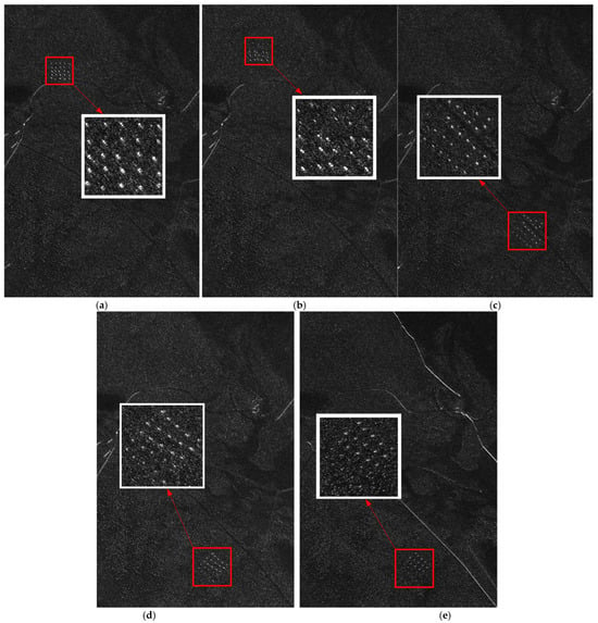
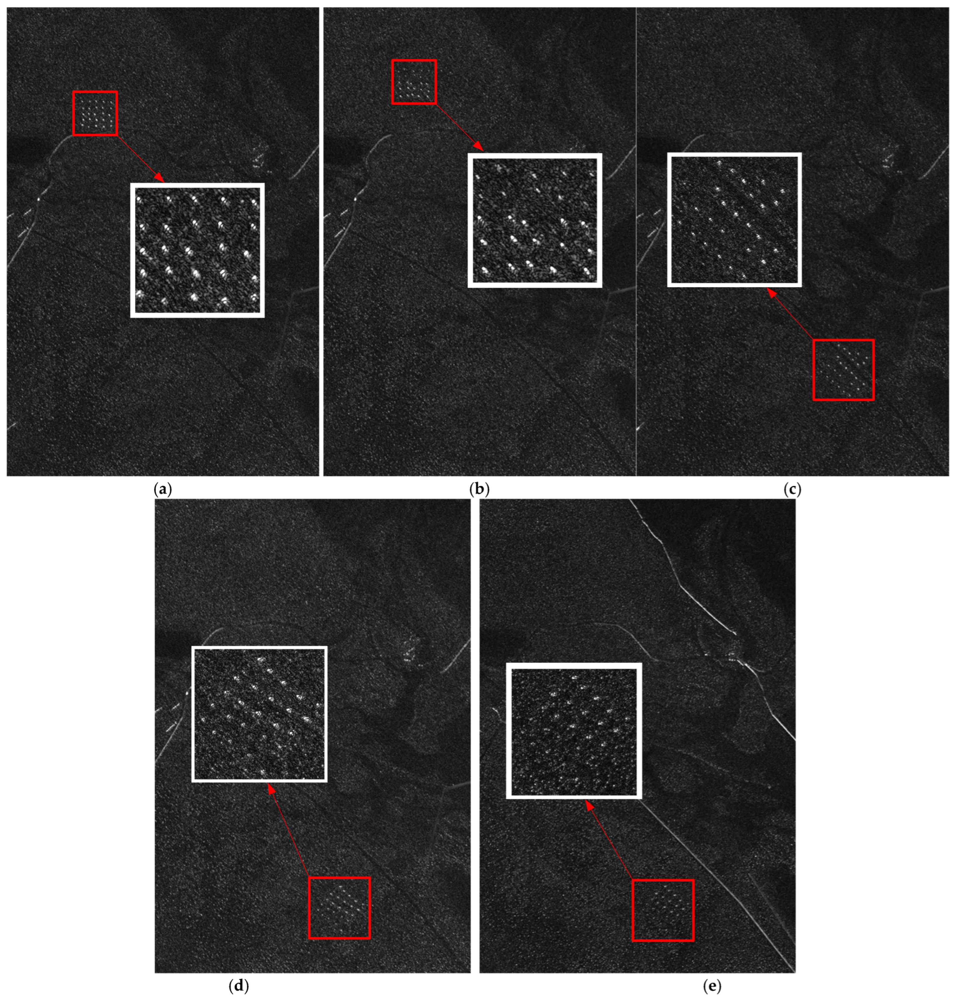
Based on headings, the 24 WRSAR images are grouped into three stacks, so that images within a stack exhibit similar background scattering statistics. Figure 1a–d illustrate vehicle position changes within a single stack, whereas Figure 1d,e highlight differences in the scattering of elongated structures under orthogonal headings.
Figure 1.
Multi-temporal and multi-heading WRSAR examples from the CARABAS-II dataset with 25 vehicle targets marked by the red square and corresponding magnification details. (a). Heading 225°, mission 1; (b) heading 225°, mission 2; (c) heading 225°, mission 3; (d) heading 225°, mission 4; (e) heading 135°, mission 4.
2.2. Multi-Angle SAR Scattering Property
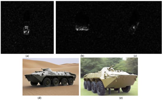
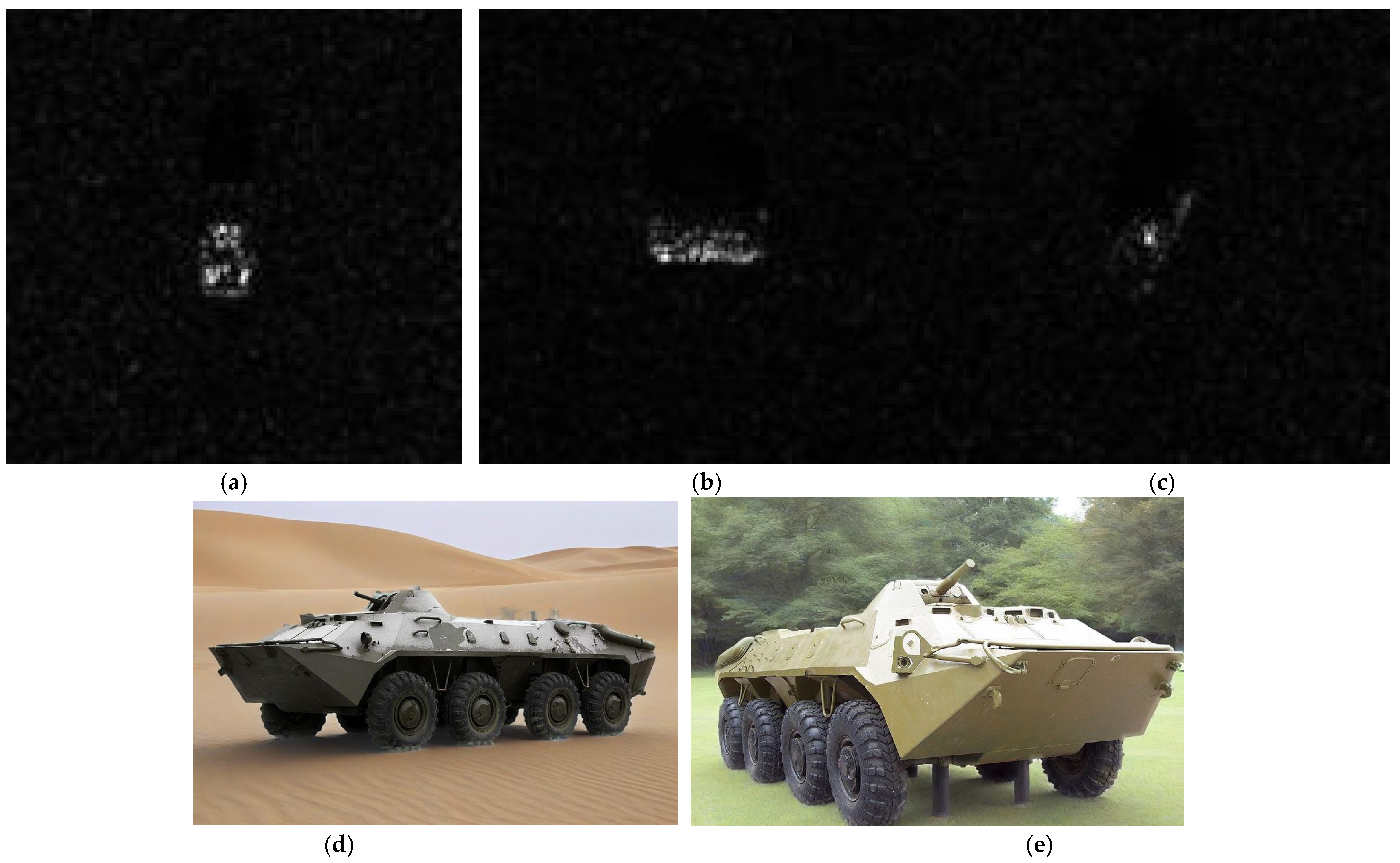
In SAR imagery, vehicle backscatter is highly aspect-dependent [21], where both the spatial distribution of intensity and the locations of bright scattering centers would vary with azimuth angle. This arises from multiple structural components—flat panels, edges, and contours—whose anisotropic reflections produce strong aspect sensitivity. Even small changes in aspect angle would induce marked fluctuations in the observed backscatter. In the MSTAR dataset [22] shown in Figure 2, the apparent shape and brightness distribution of vehicles vary with orientation, accompanied by geometric effects inherent to SAR imaging. When the long axis of the vehicle is parallel to the radar line of sight, e.g., in Figure 2a, foreshortening compresses the returns along range, shortening the apparent length. When the long axis of the vehicle is oriented towards the radar, e.g., in Figure 2b, strong mechanisms such as vehicle–ground dihedral reflections often dominate. At oblique aspects, e.g., in Figure 2c, the corner reflection would weaken, and the roof or wheels would become the primary scattering centers. Additionally, the inherent geometric distortions of SAR imaging, such as layover and shadowing, would cause the upper parts of the vehicle to be displaced forward relative to their actual ground positions and create no-return regions behind the vehicle.
Figure 2.
The multi-angle Ka-band SAR examples of BTR-70 armored vehicles from the MSTAR dataset. (a) Angle 0°; (b) angle 90°; (c) angle 45°; (d,e) optical images.
Wide-angle SAR studies [23] show that expanding the aspect coverage significantly improves the robustness of vehicle detection. Consequently, multi-angle observation offers a direct means to mitigate the limitations of single-angle imaging. By aggregating complementary viewpoints, multi-angle SAR reduces low radar cross-section (RCS) aspect gaps and enhances both target visibility and discrimination from natural clutter. In practice, multi-angle coverage is realized by imaging from different flight headings. Since the vehicle scattering is strongly aspect-dependent, single-view recognition remains challenging. Multi-heading acquisitions could explicitly address this aspect sensitivity.
2.3. WRSAR Image Statistical Property
Building on binary hypothesis testing for WRSAR imagery [9], we decide target presence on a per-pixel basis to separate FOPEN targets from the background. The hypothesis test can be expressed as
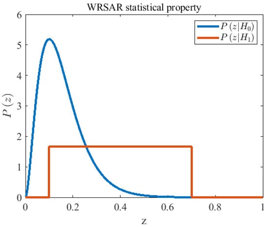
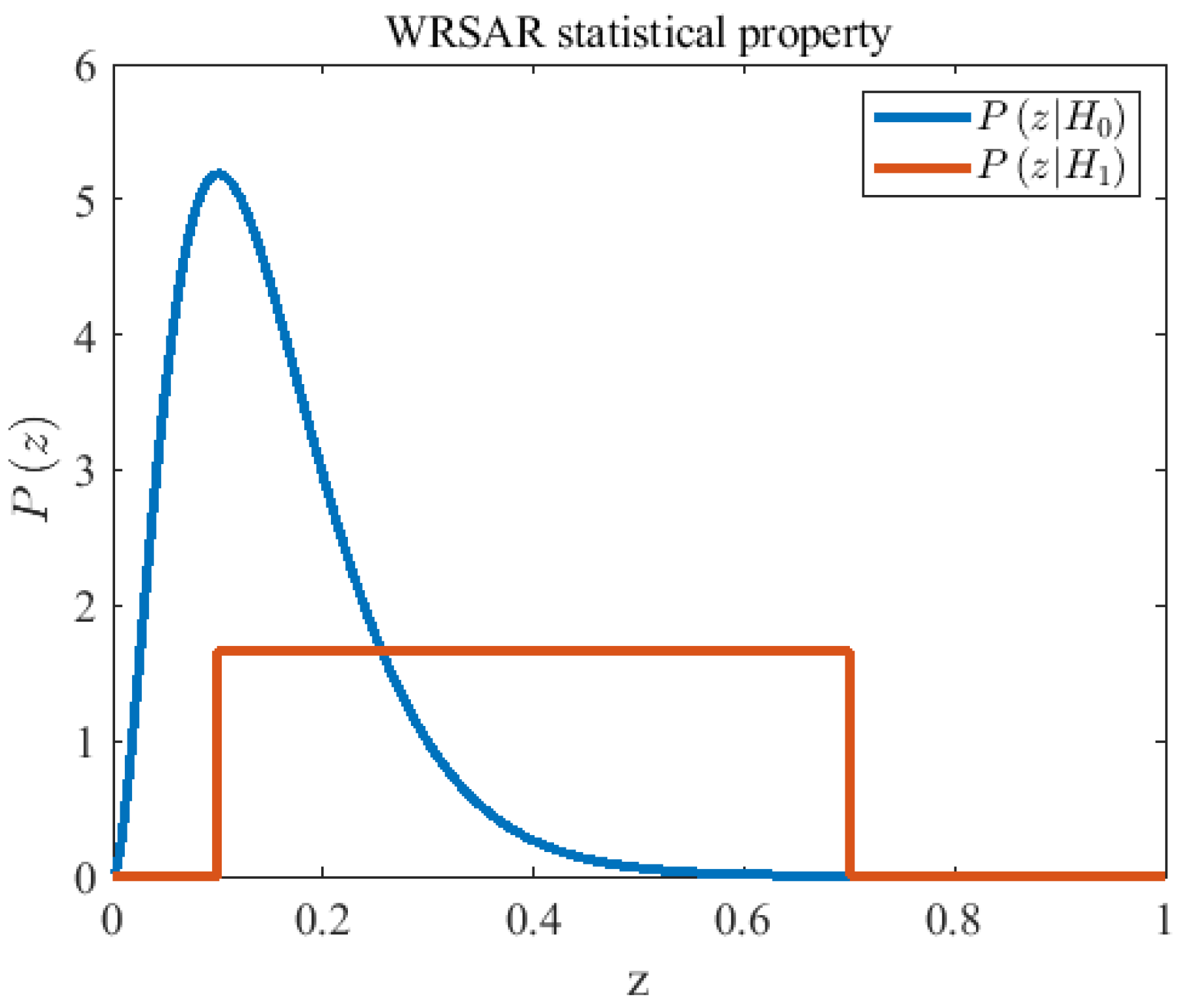
where denotes the observation at a given pixel, is the hypothesis that the evaluated pixel is background-related, is the hypothesis that the evaluated pixel is target-related (change), is related to the target, and is the clutter–noise model, in which is related to the clutter and to the noise. Figure 3 illustrates the class-conditional densities and estimated for the scene of Figure 1a where is approximated by a Gamma distribution, whereas is modeled as uniform over the dynamic range.
Figure 3.
The ideal statistical property of various regions in the WRSAR image.
3. Details About the Proposed Method
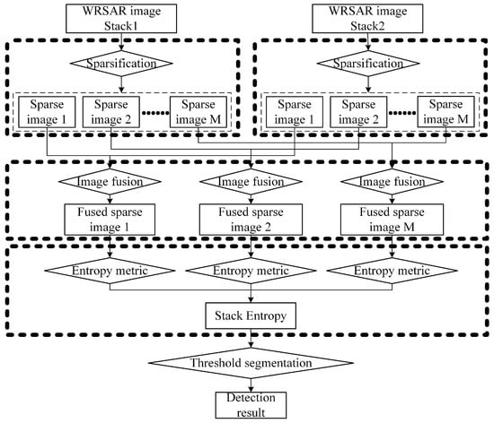
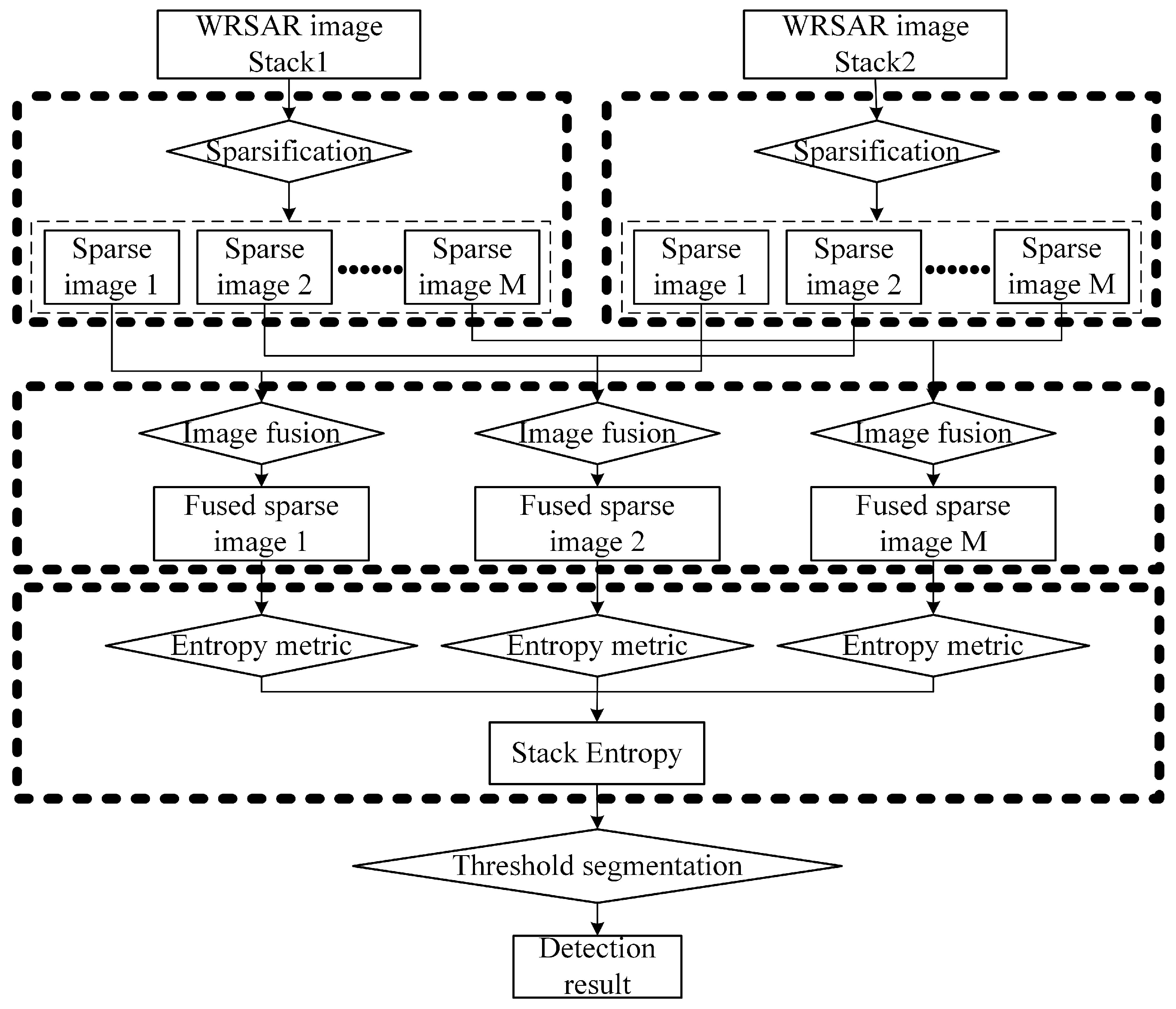
The proposed image stack fusion-based FOPEN vehicle detection (ISFFVD) framework comprises three modules: low-rank decomposition, orthogonal-heading image stack fusion, and stack entropy metrics. The overall pipeline is shown in Figure 4, where the low-rank decomposition module is highlighted in red, the image stack fusion module in green, and the stack entropy module in blue. Compared with the recent image stack-based FOPEN vehicle detection (ISFVD) [16] baseline, ISFFVD is more computationally efficient for the sparsification of WRSAR images; thus, the cost of stack entropy evaluation is substantially reduced. Motivated by the non-negativity of WRSAR amplitudes, we design a non-negative constrained tensor robust principal component analysis (NCTRPCA) to obtain non-negative clutter and target components. To accommodate vehicle anisotropy, ISFFVD fuses orthogonal-heading sparse stacks using Itakura–Saito divergence-based non-negative matrix factorization (IS-NMF), thereby enriching backscattering diversity relative to single-heading views. Finally, unlike the Shannon entropy (SE) used in ISFVD, we evaluate the fused sparse stack by the tunable Rayleigh-entropy (RE) metric to obtain a more flexible and discriminative stack statistic.
Figure 4.
The framework of the proposed ISFFVD.
3.1. Non-Negative Constrained TRPCA
For the WRSAR image stack utilized in the proposed ISFFVD, we consider the image stack as a tensor and implement TRPCA [14] by the tensor strategy, i.e.,
where is the image stack, is a low-rank tensor, and is a sparse tensor. Based on the non-negative property in (2), we should further constrain TRPCA by . In this case, we could obtain and with a tight recovery guarantee through the following optimization problem:
where is the tensor nuclear norm of , which can be computed by the sum of singular values of all frontal slices in , i.e., , where is the th frontal slice of , and is the Fourier transform result of along the tensor direction. The tensor nuclear norm [24] is induced by the tensor–tensor product, which is a generalization of the matrix–matrix product. In addition, the sparse content is computed by summing the absolute values of all contents in with balancing the content between and . According to [16], the value that exactly recovers and under certain assumptions is defined by
To solve (3), we can use the augmented Lagrangian (AL) parameter to rewrite (3) as
where represents the incoherence parameter. This augmented Lagrangian multiplier (ALM) [24] is essentially a joint optimization between variables and ; thus, we can solve it by the alternating direction method of multiplier (ADMM) and non-negative projection (NNP); i.e., the optimization process can be summarized as the following steps:
Considering NCTRPCA is based on the MATLAB 2024 implementations TRPCA in [25] with the same hyperparameter and the WRSAR image stack in this paper is consistent with it in [26], we directly utilize the existing conclusion, i.e., is equal to , . As stopping criteria in [26], we set the update threshold as and the maximum iterations as , i.e.,
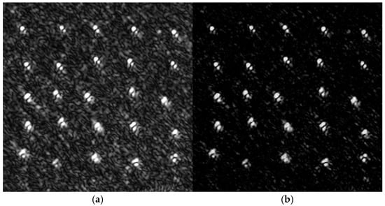
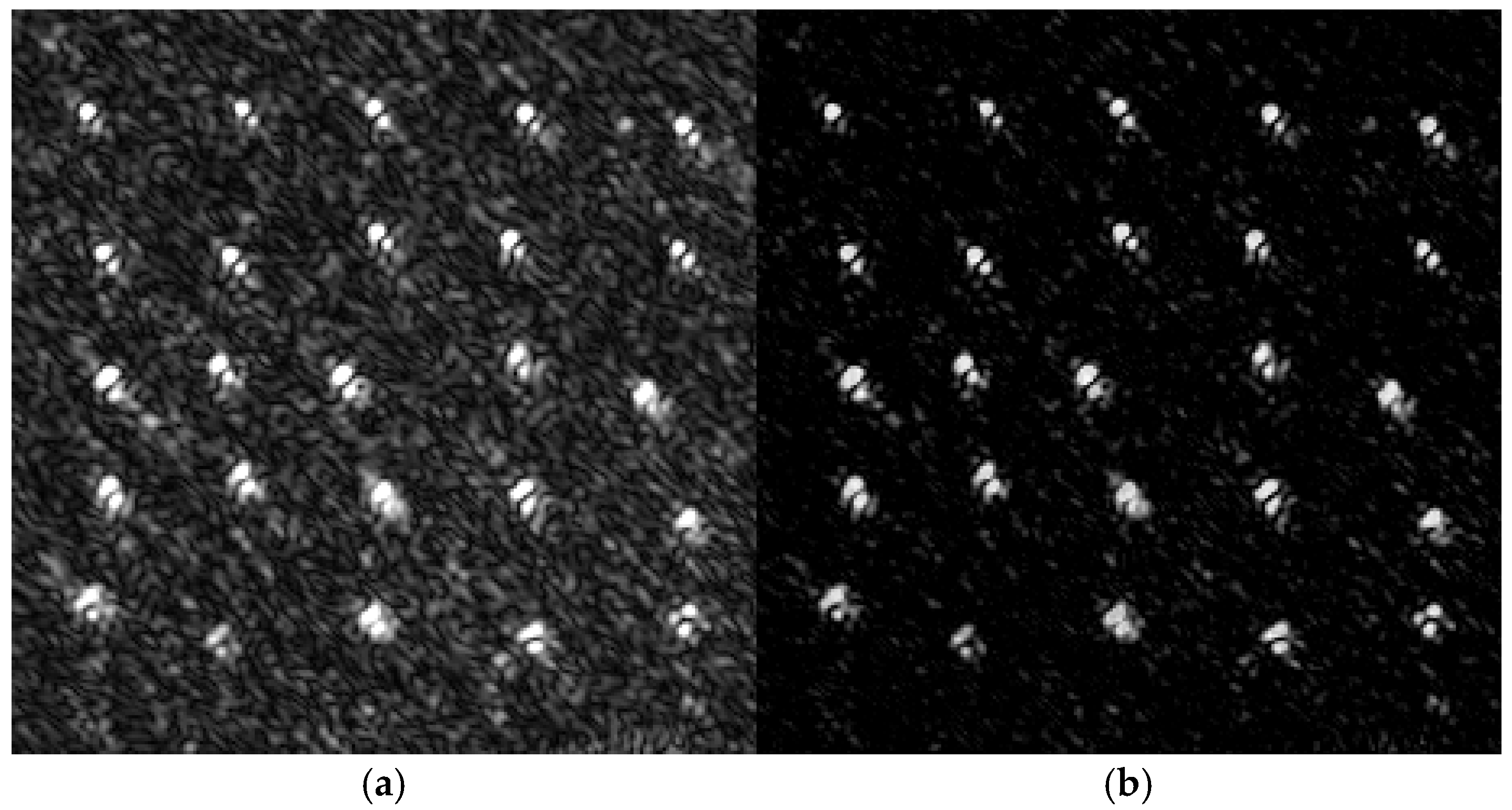
where represents the infinite norm. Figure 5 shows the low-rank matrix factorization result by NCTRPCA. From the sparse rate, i.e., zero-element ratio, we can see that NCTRPCA rapidly increases the sparse rate of WRSAR images.
Figure 5.
The low-rank factorization result of the WRSAR image at heading 225°, mission 2. (a) Original WRSAR image with 0% sparse rate; (b) sparse WRSAR image with about 73.31% sparse rate.
3.2. Itakura–Saito Divergence-Based NMF
After the NCTRPCA-based WRSAR image stack preprocessing, we obtain two orthogonal-heading sparse WRSAR image stacks. To represent the scattering property of FOPEN vehicles comprehensively, we should fuse these sparse image stacks into a new sparse image stack. To avoid overly increasing the computational complexity of the proposed ISFFVD method, we directly conduct the non-negative matrix factorization (NMF) [27] method to fuse sparse image stacks. NMF as an unsupervised matrix analytic method could iteratively extract main features from various images.
NMF is essentially to decompose a large-scale matrix with - dimensional features into two small large-scale matrices, and , such that
where is defined as the basis matrix with the free parameter and is the coefficient matrix that approximately reconstructs the original - dimension feature from the decreased - dimensional feature. As we expand images into several column vectors like and set = 1, the basis matrix could be considered as the fused result of images in . In the traditional compressed sensing, the Frobenius distance could be taken to minimize the reconstruction error , i.e.,
by the multiplicative update rule where is usually a non-sparse matrix.
Regarding the sparse WRSAR image fusion, we select the Itakura–Saito divergence [28], which is widely utilized to analyze the sparse power spectrum, i.e.,
Setting , the partial derivative of (10) can be written as
where represents the dot product and , represents the element-wise exponentiation of . Similar with the Lee–Seung multiplicative update rule, we can optimize and iteratively as
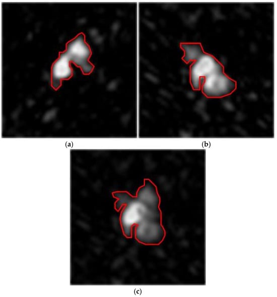
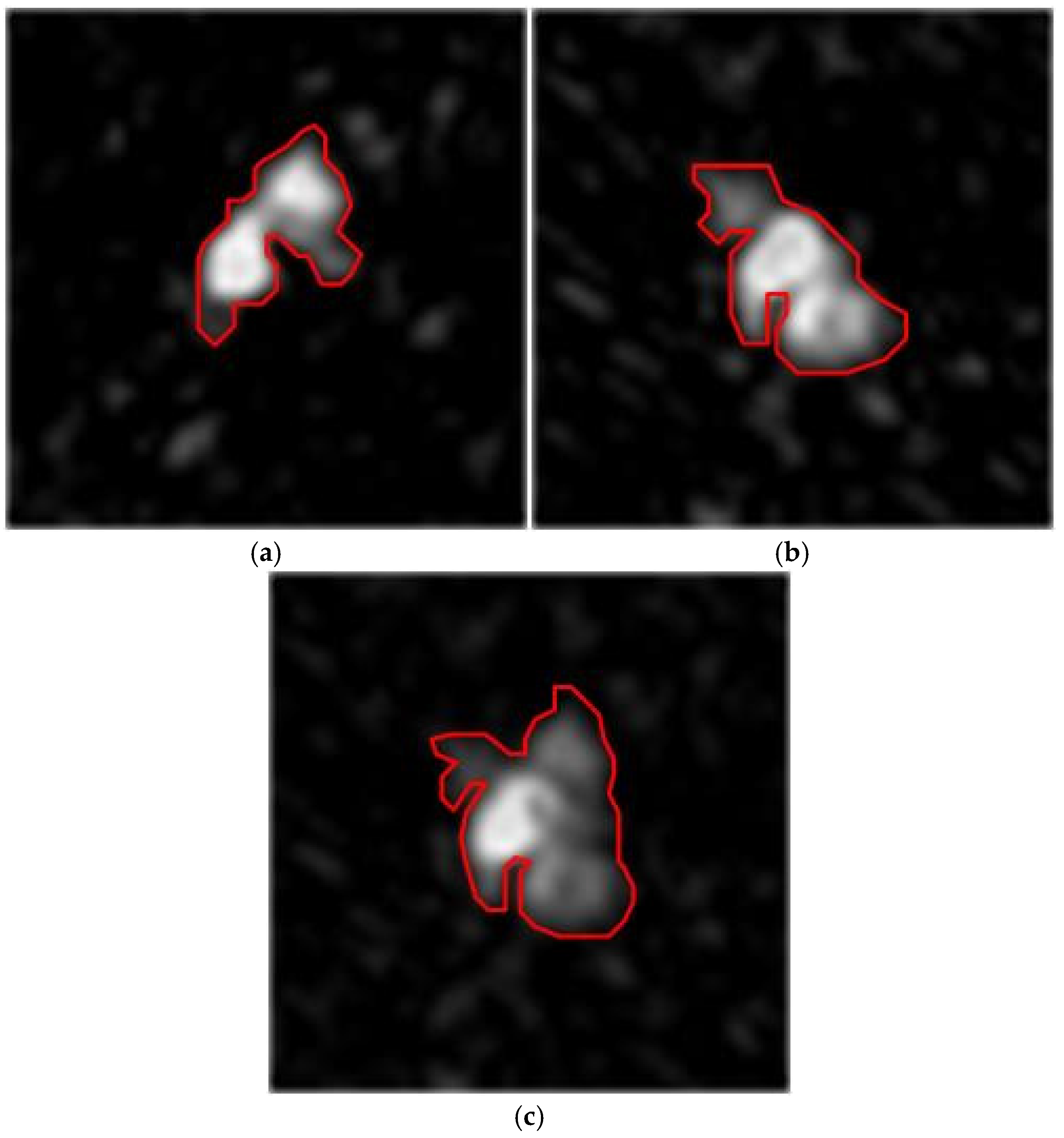
Figure 6 shows the detailed WRSAR imaging result of the vehicle at orthogonal headings, where we sketched the outline of the target with red lines. Figure 6a illustrates the scattering property of the long-axis side of the vehicle, while Figure 6b illustrates the scattering property of the short-axis side of the vehicle. Since the WRSAR system at a single heading only obtains the local scattering property of the target, the vehicle shows a narrow shape in the imaging result. Compared with Figure 6a,b, the fused orthogonal heading could obtain rich scattering properties; thus, the vehicle is comprehensively displayed in Figure 6c.
Figure 6.
Orthogonal-heading WRSAR images with the target coverage area marked in red and their fusion results. (a) Target at heading 225°; (b) target at heading 135°; (c) orthogonal heading fusion result.
3.3. Rényi Entropy-Based Statistic Metric
The stack entropy statistic in the proposed ISFFVD is to compute and compare the entropy of all images in the fused sparse WRSAR image stack. To estimate distribution parameters by the maximum likelihood estimation (MLE), we perform a sliding window traversal of the image pixel according to square-shaped regions of interest (ROIs) of side length centered around each pixel of the image. Set as the size of the ROI. The entropy statistic of the ROI is considered as that of the central pixel, and the side length can be set as the minimum target interval. To calculate the statistical expression of Rényi entropy (RE) in ROIs, we should obtain the parameter of the pixel distribution. In this paper, we give the Gamma distribution-based expression of the RE statistic metric.
Assuming the sample for in ROIs obeys the Gamma distribution, the probability density function is
where is the shape parameter and is the rate parameter. Rewriting (13) to the log-likelihood form, we can obtain
Taking the partial derivative of and setting it to zero, we get
where is the Gamma function and . In addition, taking MLE-based into the partial derivative of , we can acquire
that is to say,
where is the Digamma function. Given that (17) has no analytical solution, we solve it iteratively using the Newton–Raphson method, i.e.,
where is the derivative of and
with the Trigamma function .
Furthermore, we can define RE as
where > 0, , and . Then, we can calculate the integral as
Based on the Gamma integral, we can get
Setting and , we can describe (22) as
Thus,
Taking (24) to (20), we estimate RE as
and it would degenerate into SE as approaches 1.
Based on [29], the difference in RE, i.e., , would converge to the Gaussian distribution, i.e., the sliding region of an ROI satisfies
where are the MLE estimate of the theoretical and is the size of the ROI. For the WSAR image stack in this paper, each ROI includes image slices, which have the same in theory; thus, we can define the theoretical RE in each ROI as
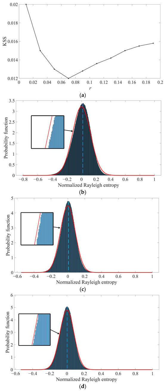
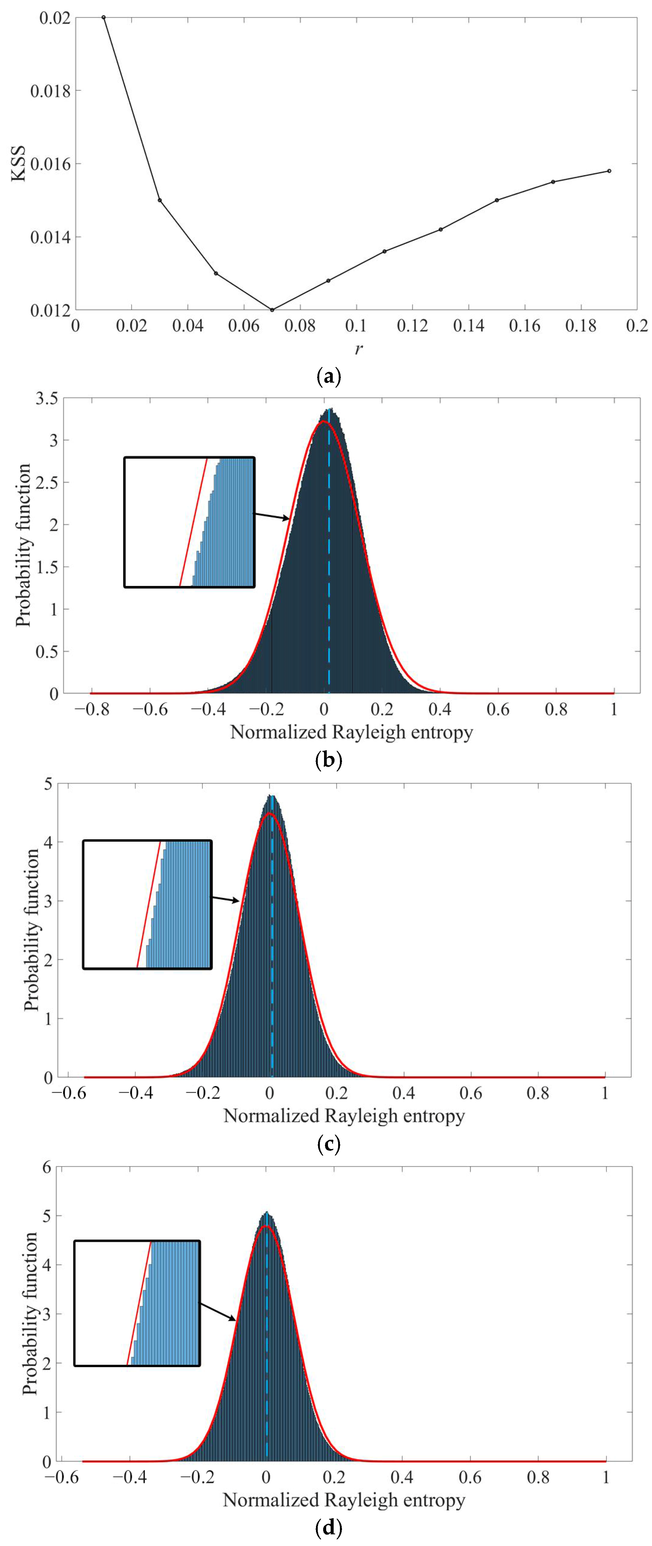
Therefore, based on the sliding window, we estimate the RE of each pixel. In addition, we should select a proper to make the distribution of the estimated RE closer to the ideal Gaussian distribution. Figure 7 illustrates the similarity between the theoretical RE distribution and actual RE distribution of Figure 1a–d, where the theoretical RE distribution, i.e., Gaussian distribution, can be calculated by MLE. Using the exhaustive method, we measure the similarity between the theoretical result and actual result by the Kolmogorov–Smirnov statistic (KSS) [30], e.g., Figure 7a, where a small KSS represents a high similarity. In addition, we can learn from Figure 7b,c that a small or a large would skew the theoretical RE distribution; e.g., and would generate a left-skewed property, where RE at is equal to SE. Under the optimal , we can see that the theoretical RE distribution and estimated RE distribution have a slight skew in Figure 7d. Therefore, the RE at is selected to describe the difference in the WRSAR image stack.
Figure 7.
The similarity of the actual RE statistical distribution and its theoretical Gaussian distribution. (a) KSS with various ; (b) with ; (c) with; (d) with .
Furthermore, the asymptotic variance approximation of the RE is performed by the Delta method [31] to obtain an accurate . This approximation assumes that the MLE estimates of the Gamma distribution parameters satisfy asymptotic normality. Performing a first-order Taylor expansion, we obtain an approximate normality of the estimated RE where its variance is expressed as a quadratic form involving the gradient of the entropy function and the covariance matrix of the parameter estimates, i.e., the inverse Fisher information matrix. Thus, the Delta method-based asymptotic variance can be approximated as follows:
where represents the Fisher information matrix (FIM) [32] of the Gamma distribution, i.e.,
Then, computing the partial derivatives of , we obtain the partial derivative with respect to and as follows:
For brevity, we commonly express (30) as
According to the matrix inversion formula, the covariance matrix of Gamma distribution parameters, i.e., , could be denoted as
Taking (31) and (32) into (28), the asymptotic variance approximation of the RE is
where , and it would transform into the variance approximation of the Shannon entropy as .
In practice, the RE is the general form of the Shannon differential entropy; thus, (25) and (33) can flexibly measure the WRSAR image stack. For simplicity, we will omit the dependence of and in the following. The null and alternative hypotheses of WRSAR images are
Considering the sum of the squares of independent standard normal random variables subject to the chi-square distribution [33], i.e.,
where the approximated can be obtained by (27). Then, we can define the RE-based statistic to represent the position change in vehicles in the WRSAR image stack as
Notably, the distribution of non-zero pixels in the aforementioned sparse WRSAR image stack follows an approximate exponential distribution, i.e., the shape parameter in (13) can be directly set to . In addition, we can also obtain the RE metrics of sparse WRSAR image stack by setting in (25) and (33). Omitting the iterative quasi-Newton estimation of in (19), the process of estimating stack entropy would be simple and efficient.
4. Experimental Result and Analysis
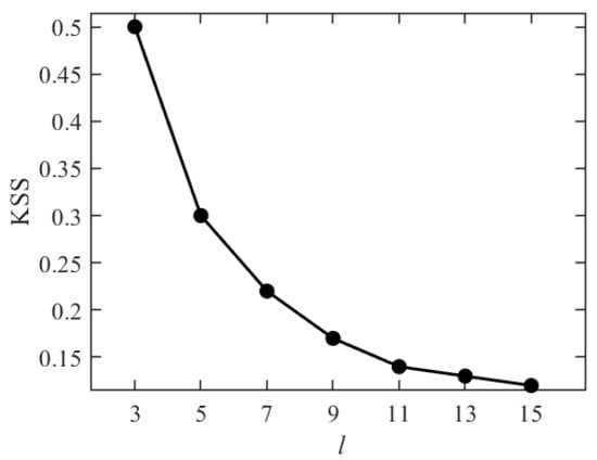
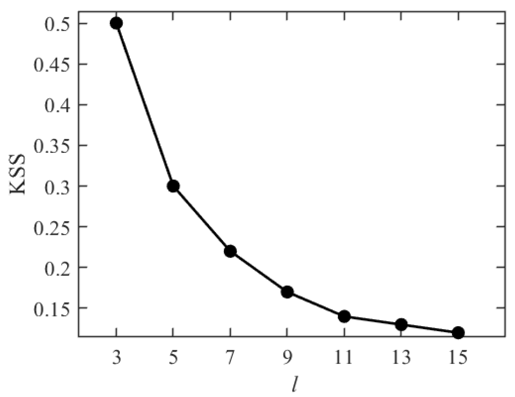
This section reports the WRSAR detection result for the state-of-the-art ISFVD and the proposed ISFVD evaluated by the Rayleigh-entropy metric with . Actually, ISFVD contains the ISFVD with single-stack entropy (ISFVD-SSE) and the ISFVD with median-stack entropy (ISFVD-MSE). Experiments use WRSAR stacks acquired at orthogonal headings (135° and 225°). In addition, each image stack contains four WRSAR images acquired at four different times, and FOPEN military vehicles would move at the time interval. Considering that the minimum inter-vehicle spacing is about 20 pixels and the largest coverage scope of vehicle is 10 × 10, the square region of interest (ROI) side length is set to . Based on the KSS-based sensitivity analysis in Figure 8, the similarity between the actual statistical distribution and the estimated statistical distribution within the ROI tends to stabilize as and the computational complexity of statistical distribution estimation as the increase of . Therefore, is the most appropriate selection in the proposed ISFFVD.
Figure 8.
The sensitivity analysis of ROI size with various side lengths .
4.1. The Stack Entropy Analysis
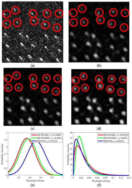
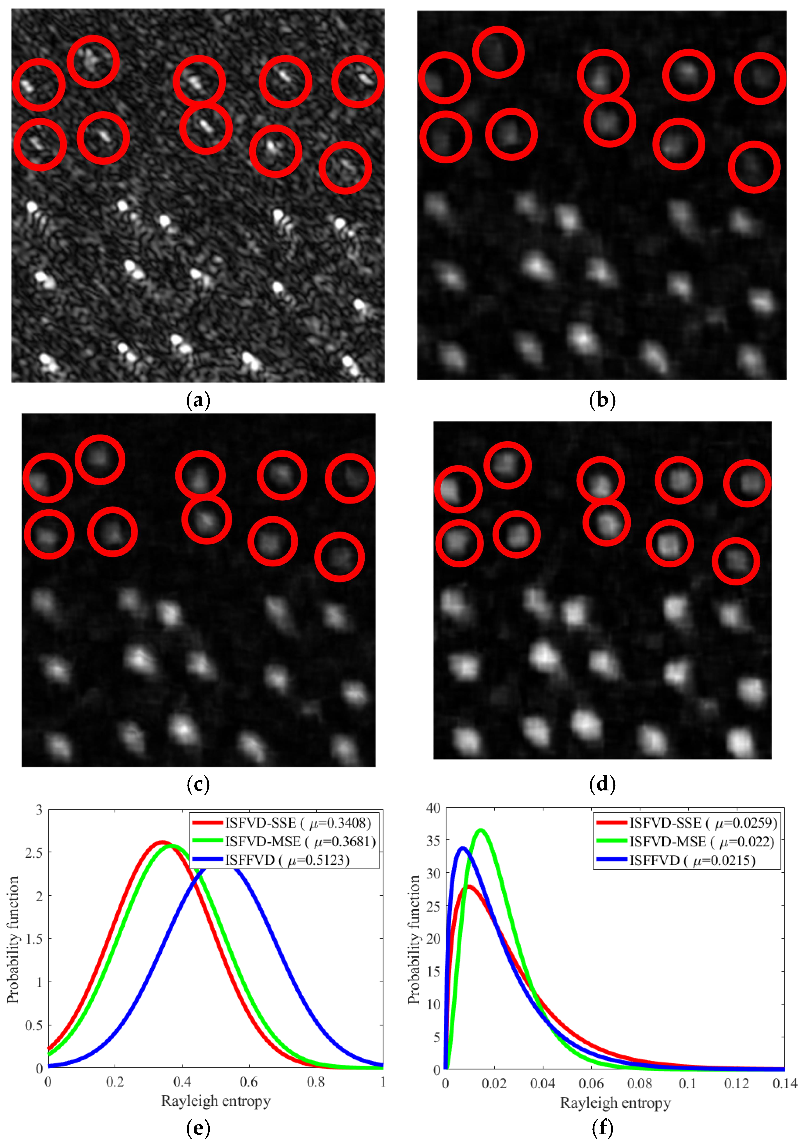
Stack entropy is central to encoding the discontinuous positional changes in FOPEN targets. Compared with the SE statistics used in the state-of-the-art ISFVD methods, i.e., ISFVD-SSE and ISFVD-MSE, the RE metric adopted in ISFFVD provides a more discriminative representation of target motion. ISFVD-SSE computes stack entropy from a single-heading WRSAR stack, whereas ISFVD-MSE takes the median of stack entropies over three headings (135°, 225°, and 230°). In addition, by the sparsification of WRSAR stacks, ISFFVD substantially reduces the computational cost of stack entropy evaluation relative to ISFVD-MSE.
Figure 9 illustrates vehicle representations obtained with ISFVD-SSE, ISFVD-MSE, and ISFFVD. Relative to the original WRSAR image, the stack entropy metric would enlarge the apparent spatial support of FOPEN targets and suppress background clutter and noise; e.g., the target regions marked by red circles in Figure 9b–d occupy more pixels than those in Figure 9a. Figure 9e,f further show the estimated pixel-value distributions for ISFVD-SSE, ISFVD-MSE, and ISFFVD over target and background regions. The probability distribution used to model the background pixels is the Gamma distribution function, and the probability distribution used to model the target pixels is the Gaussian function. The mathematical expectation of each distribution serves as an energy indicator for the corresponding region of interest. Combining these distributions with the visual representations, we can learn that compared with ISFVD-SSE and ISFVD-MSE, ISFFVD significantly enhances the energy of the target region in the representation result and maintains the low energy of the background region; thus, the target in the ISFFVD result, i.e., the red-circle region in Figure 9d, could be clearly represented.
Figure 9.
The image stack entropy-based vehicle representation results in a local area with 10 weakly scattered targets marked by red circles among the 25 targets (a) Original WRSAR image; (b) ISFVD-SSE result; (c) ISFVD-MSE result; (d) proposed ISFFVD result; (e) the target pixel distribution; (f) the background pixel distribution.
4.2. The Detection Result Analysis
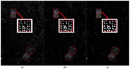
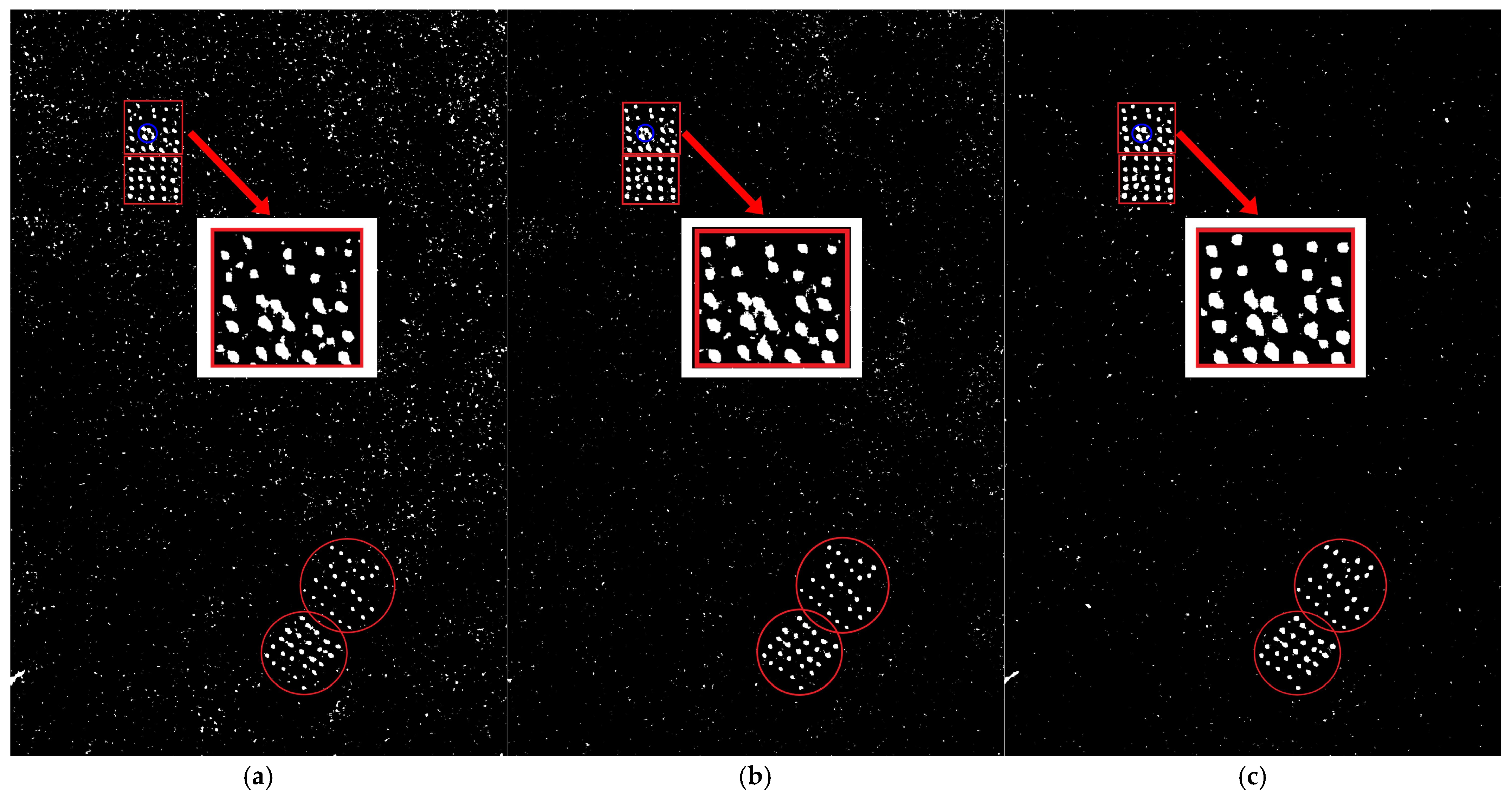
Based on the estimated pixel distribution over targets and background regions, we can perform maximum a posteriori (MAP) criterion on each stack entropy representation to detect FOPEN vehicles where MAP is implemented in a global manner. Figure 10 shows detection results without morphological post-processing. In this scene, 25 military vehicles (five per convoy across five rows) move to four distinct positions over four time instants, highlighted by red boxes. Under the MAP criterion, all three methods, i.e., ISFVD-SSE, ISFVD-MSE, and ISFFVD, successfully detect the vehicles. However, ISFFVD yields fewer false alarms in background areas and preserves sharper target boundaries in local zoom-ins. In contrast, the detection results from ISFVD-SSE and ISFVD-MSE exhibit blurred edges (marked by the blue circle), indicating lower effective spatial resolution capability.
Figure 10.
The FOPEN vehicle detection result from various image stack entropy-based representations according to the MAP criterion. (a) ISFVD-SSE result; (b) ISFVD-MSE result; (c) ISFFVD result.
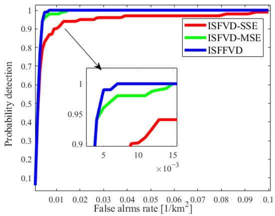
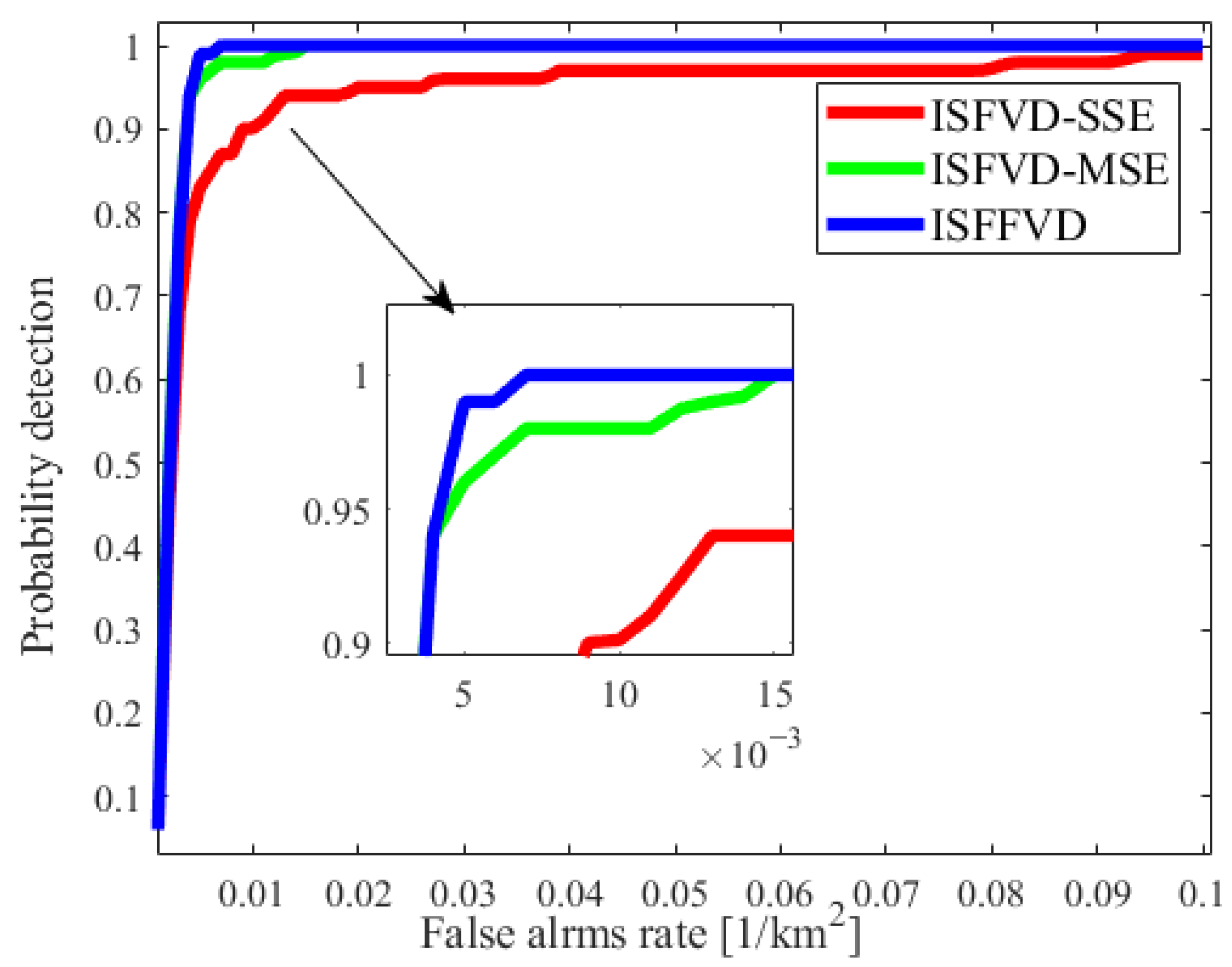
Performance is further summarized via receiver operating characteristic (ROC) curves [34] and parameterized by detection probability (PD) and false alarm rate (FAR). Here, PD denotes the fraction of true targets correctly declared, and FAR denotes the proportion of background pixels falsely declared as targets, normalized per square kilometer. Figure 11 reports ROC curves for ISFVD-SSE, ISFVD-MSE, and ISFFVD over the operating range . Within this range, we can learn that ISFFVD outperforms ISFVD-SSE as and outperforms ISFVD-MSE as . The areas under curves (AUCs) in Table 1 confirm that ISFFVD achieves the largest AUC, indicating superior overall performance.
Figure 11.
ROC curves obtained from ISFVD-SSE, ISFVD-MSE, and ISFFVD methods with and .
Table 1.
The execution time of various methods within different modules.
We also compare the execution time of the three-stack entropy-based FOPEN vehicle detection method in Table 1, where the total time also includes the preprocessing time. ISFFVD consists of three modules—the LRSF module, ISF module, and SEM module—whereas ISFVD-SSE and ISFVD-MSE need only SEM. As shown in Table 1, ISFVD-SSE based on single-heading WRSAR image stack is the fastest, and ISFVD-MSE based on three WRSAR image stacks requires roughly three times longer than ISFVD-SSE. Although ISFFVD includes two additional modules, sparsification produced by LRSF substantially accelerates the subsequent SEM stage (13 s vs. 64 s), and ISF makes ISFFVD require computing Rayleigh entropy for only one fused image stack in the SEM stage. Consequently, the total runtime of ISFFVD is heavier than ISFVD-SSE but markedly lower than ISFVD-MSE. Considering MAP detection results, AUCs, and runtime jointly, ISFFVD offers the best accuracy–efficiency trade-off.
5. Conclusions
This paper introduces orthogonal-heading WRSAR stack fusion into entropy-based FOPEN target detection for the first time, in order to enhance the saliency and energy concentration of concealed targets. The key idea is to apply a low-rank–sparse decomposition to multi-temporal image stacks and to compute the stack entropy directly on the sparse component, thereby preserving discriminative power while markedly reducing computational cost. In addition, Rayleigh entropy is adopted as a generalized alternative to Shannon entropy, which better matches the scattering statistics under dense canopy and yields a more faithful characterization of concealed targets. Experimental results show that the proposed fused-stack detector achieves a higher detection rate with an acceptable overall runtime, striking a favorable balance between accuracy and efficiency. The experimental validation in this paper is conducted on the publicly available CARABAS-II dataset, which is widely used in the VHF-band FOPEN SAR literature. Consequently, the adaptability of the proposed representation to more complex terrains (e.g., mountainous areas, wetlands) and its generalization to other radar systems and acquisition conditions cannot yet be comprehensively verified. We are actively developing the P-band and L-band FOPEN radar system and plan to build a larger self-collected dataset covering diverse terrain types and operational scenarios. Future work will evaluate the proposed change-difference map generation on these datasets and further explore its integration with learning-based detectors.
Author Contributions
Conceptualization, H.Z.; methodology, H.Z.; software, H.Z.; validation, H.Z.; formal analysis, H.Z.; investigation, H.Z.; resources, D.A.; data curation, H.Z.; writing—original draft preparation, H.Z.; writing—review and editing, H.Z.; visualization, H.Z.; supervision, D.A.; project administration, D.A.; funding acquisition, D.A. All authors have read and agreed to the published version of the manuscript.
Funding
This work was supported in part by the National Natural Science Foundation of China under Grant 62271492.
Data Availability Statement
The original data presented in this study can be publicly accessed in the Sensor Data Management System (sdms) of Air Force Research Laboratory (AFRL) at the https://www.sdms.afrl.af.mil/index.php?collection=vhf_change_detection accessed on 20 October 2025 and https://www.sdms.afrl.af.mil/index.php?collection=mstar accessed on 13 November 2025.
Acknowledgments
We would like to thank Daoxiang An for providing financial support.
Conflicts of Interest
The authors declare no conflicts of interest.
References
- Hellsten, H.; Froelind, P.-O.; Gustafsson, A.; Jonsson, T.; Larsson, B.; Stenstroem, G.; Binder, B.T.; Mirkin, M.I.; Ayasli, S. Ultrawideband VHF SAR design and measurements. In Proceedings of the SPIE’S International Symposium on Optical Engineering and Photonics in Aerospace Sensing, Orlando, FL, USA, 4–8 April 1994; SPIE: Bellingham, WA, USA, 1994; Volume 2217, pp. 6–26. [Google Scholar]
- Machado, R.; Vu, V.T.; Pettersson, M.I.; Dammert, P.; Hellsten, H. The stability of UWB low-frequency SAR images. IEEE Geosci. Remote Sens. Lett. 2016, 13, 1114–1118. [Google Scholar] [CrossRef] [Scilit]
- Xie, H.; Zhang, Y.; He, J.; Yi, S.; Zhang, L.; Zhu, N. Foliage-concealed target change detection scheme based on convolutional neural network in low-frequency ultrawideband SAR images. IEEE J. Sel. Top. Appl. Earth Obs. Remote Sens. 2024, 17, 19302–19316. [Google Scholar] [CrossRef] [Scilit]
- Alves, D.I.; Palm, B.G.; Pettersson, M.I.; Vu, V.T.; Machado, R.; Uchoa-Filho, B.F.; Dammert, P.; Hellsten, H. A statistical analysis for wavelength-resolution SAR image stacks. IEEE Geosci. Remote Sens. Lett. 2020, 17, 227–231. [Google Scholar] [CrossRef] [Scilit]
- Hellsten, H.; Ulander, L.M.H.; Gustavsson, A.; Larsson, B. Development of VHF CARABAS II SAR. In Proceedings of the Aerospace/Defense Sensing and Controls, Orlando, FL, USA, 8–12 April 1996; SPIE: Bellingham, WA, USA, 1996; Volume 2747, pp. 48–60. [Google Scholar]
- Alves, D.I. Change detection for low-frequency SAR ground surveillance. IEE Proc.-Radar Sonar Navig. 2005, 1352, 413–420. [Google Scholar]
- Vu, V.T.; Gomes, N.R.; Pettersson, M.I.; Dammert, P.; Hellsten, H. Bivariate gamma distribution for wavelength-resolution SAR change detection. IEEE Trans. Geosci. Remote Sens. 2019, 57, 473–481. [Google Scholar] [CrossRef] [Scilit]
- Gomes, N.R.; Dammert, P.; Pettersson, M.I.; Vu, V.T.; Hellsten, H. Comparison of the Rayleigh and K-distributions for application in incoherent change detection. IEEE Geosci. Remote Sens. Lett. 2019, 16, 756–760. [Google Scholar] [CrossRef] [Scilit]
- Alves, D.I.; Müller, C.; Palm, B.G.; Pettersson, M.I.; Vu, V.T.; Machado, R.; Uchôa-Filho, B.F.; Dammert, P.; Hellsten, H. Neyman-Pearson criterion-based change detection methods for Wavelength-resolution SAR image stacks. IEEE Geosci. Remote Sens. Lett. 2022, 19, 1–5. [Google Scholar] [CrossRef] [Scilit]
- Hellsten, H.; Machado, R.; Pettersson, M.I.; Vu, V.T.; Dammert, P. Experimental results on change detection based on Bayes probability theorem. In Proceedings of the IEEE International Geoscience and Remote Sensing Symposium (IGARSS), Milan, Italy, 26–31 July 2015; pp. 318–321. [Google Scholar]
- Hellsten, H.; Machado, R. Bayesian change analysis for finding vehicle size targets in VHF foliage penetration SAR data. In Proceedings of the IEEE Radar Conference, Johannesburg, South Africa, 27–30 October 2015; pp. 510–515. [Google Scholar]
- Vu, V.T.; Pettersson, M.I.; Machado, R.; Dammert, P.; Hellsten, H. False alarm reduction in wavelength-resolution SAR change detection using adaptive noise canceler. IEEE Trans. Geosci. Remote Sens. 2017, 55, 591–599. [Google Scholar] [CrossRef] [Scilit]
- Vu, V.T.; Pettersson, M.I.; Dammert, P.; Hellsten, H. Two-dimensional data conversion for one-dimensional adaptive noise canceler in low-frequency SAR change detection. IEEE Trans. Aerosp. Electron. Syst. 2018, 54, 2611–2618. [Google Scholar] [CrossRef] [Scilit]
- Ramos, L.P.; Alves, D.I.; Duarte, L.T.; Machado, R.; Pettersson, M.I.; Vu, V.T.; Dammert, P. Change detection in wavelength-resolution SAR image stack based on tensor robust PCA. IEEE Geosci. Remote Sens. Lett. 2024, 21, 1–5. [Google Scholar] [CrossRef] [Scilit]
- Ramos, L.P.; Campos, A.B.; Schwartz, C.; Duarte, L.T.; Alves, D.I.; Pettersson, M.I.; Vu, V.T.; Machado, R. A wavelength-resolution SAR change detection method based on image stack through Robust Principal Component analysis. Remote Sens. 2021, 13, 833. [Google Scholar] [CrossRef] [Scilit]
- Vinholi, J.G.; Silva, P.R.B.d; Alves, D.I.; Machado, R. Enhancing change detection in ultra-wideband VHF SAR imagery: An entropy-based approach with median ground scene masking. IEEE Trans. Geosci. Remote Sens. 2024, 62, 1–15. [Google Scholar] [CrossRef] [Scilit]
- Machado, R.; Vu, V.T.; Pettersson, M.I.; Dammert, P.; Hellsten, H. Change detection in SAR images using hypothesis testing and Shannon entropy based on the Rayleigh distribution. IEEE Trans. Geosci. Remote Sens. 2025, 63, 1–12. [Google Scholar]
- Vinholi, J.G.; Palm, B.G.; Silva, D.; Machado, R.; Pettersson, M.I. Change detection based on convolutional neural networks using stacks of wavelength-resolution synthetic aperture radar images. IEEE Trans. Geosci. Remote Sens. 2022, 60, 1–14. [Google Scholar] [CrossRef] [Scilit]
- Vint, D.; Anderson, M.; Yang, Y.; Ilioudis, C.; Di Caterina, G.; Clemente, C. Automatic target recognition for low resolution foliage penetrating SAR images using CNNs and GANs. Remote Sens. 2021, 13, 596. [Google Scholar] [CrossRef] [Scilit]
- Bobkov, S.G.; Chistyakov, G.P. Entropy Power Inequality for the Rényi Entropy. IEEE Trans. Inf. Theory 2015, 61, 708–714. [Google Scholar] [CrossRef] [Scilit]
- Li, W.; Ma, Y.; Zhang, Y.; Li, B.; Shi, Y.; Chu, L. A multiangle observation and imaging method for UAV swarm SAR based on consensus constraints. IEEE Sens. J. 2025, 25, 4558–4575. [Google Scholar] [CrossRef] [Scilit]
- Liu, Z.; Luo, S.; Wang, Y. Mix MSTAR: A synthetic benchmark dataset for multi-class rotation vehicle detection in large-scale SAR images. Remote Sens. 2023, 15, 4558. [Google Scholar] [CrossRef] [Scilit]
- Li, J.; An, D.; Feng, D.; Xu, J.; Chen, L.; Zhou, Z. Full-angle DEM generation based on repeat-pass L-band CSAR interferometry-theory and experimental results. IEEE Sens. J. 2024, 24, 3301–3316. [Google Scholar] [CrossRef] [Scilit]
- Lu, C.; Feng, Y.; Chen, Y.; Liu, W.; Lin, Z.; Yan, S. Tensor robust principal component analysis with a new tensor nuclear norm. IEEE Trans. Pattern Anal. Mach. Intell. 2020, 42, 925–938. [Google Scholar] [CrossRef] [Scilit]
- Lu, C. Tensor Robust PCA. Available online: https://github.com/canyilu/Tensor-Robust-Principal-Component-Analysis-TRPCA (accessed on 3 October 2022).
- Ramos, L.P.; Alves, D.I.; Duarte, L.T.; Pettersson, M.I.; Machado, R. Robust principal component analysis techniques for ground scene estimation in SAR imagery. IEEE J. Sel. Top. Appl. Earth Obs. Remote Sens. 2023, 15, 9697–9710. [Google Scholar] [CrossRef] [Scilit]
- Lee, D.; Seung, H. Algorithms for non-negative matrix factorization. In Proceedings of the Neural Information Processing Systems (NeurIPS), Denver, CO, USA, 28–30 November 2000; MIT Press: Cambridge, MA, USA, 2000; pp. 1–7. [Google Scholar]
- Bertin, N.; Fevotte, C.; Badeau, R. A tempering approach for Itakura-Saito non-negative matrix factorization. With application to music transcription. In Proceedings of the IEEE International Conference on Acoustics, Speech and Signal Processing (ICASSP), Taipei, Taiwan, 26–31 July 2009; pp. 1545–1548. [Google Scholar]
- Pardo, L.; Morales, D.; Salicrú, M.; Menéndez, M.L. Large sample behavior of entropy measures when parameters are estimated. Commun. Stat. Theory Methods 1997, 26, 483–501. [Google Scholar] [CrossRef] [Scilit]
- Priest, D.J.D. Testing goodness-of-fit for the singly truncated normal distribution using the Kolmogorov-Smirnov statistic. IEEE Trans. Geosci. Remote Sens. 1983, 21, 441–446. [Google Scholar] [CrossRef]
- Beutner, E. Delta method, asymptotic distribution. In Wiley Interdisciplinary Reviews: Computational Statistics; Wiley: Hoboken, NJ, USA, 2023; Volume 16, pp. 1634–1648. [Google Scholar]
- Pakrooh, P.; Pezeshki, A.; Scharf, L.L.; Cochran, D.; Howard, S.D. Analysis of Fisher information and the Cramér-Rao bound for nonlinear parameter estimation after random compression. IEEE Trans. Signal Process. 2015, 63, 6423–6428. [Google Scholar] [CrossRef] [Scilit]
- Salicrú, M.; Menéndez, M.L.; Morales, D.; Pardo, L. Asymptotic distribution of (h,φ)-entropies. Commun. Stat. Theory Methods 1993, 22, 2015–2031. [Google Scholar] [CrossRef] [Scilit]
- Kay, S. Fundamentals of Statistical Signal Processing: Detection Theory; Prentice-Hall: Upper Saddle River, NJ, USA, 1998. [Google Scholar]

Disclaimer/Publisher’s Note: The statements, opinions and data contained in all publications are solely those of the individual author(s) and contributor(s) and not of MDPI and/or the editor(s). MDPI and/or the editor(s) disclaim responsibility for any injury to people or property resulting from any ideas, methods, instructions or products referred to in the content. |
© 2026 by the authors. Licensee MDPI, Basel, Switzerland. This article is an open access article distributed under the terms and conditions of the Creative Commons Attribution (CC BY) license.