


Highlights
What are the main findings?
- Satellite-derived XCO2 exhibits strong hemispheric asymmetry, with fourfold-larger seasonal amplitude in the Northern Hemisphere than in the Southern Hemisphere and a consistent one-month lag of oceanic signals relative to land.
- Despite higher atmospheric CO2 growth rates over coastal regions, sea surface pCO2 increases more slowly there than in the open ocean, indicating a buffering effect of marginal seas.
What are the implications of the main findings?
- Integrating satellite XCO2 with ocean pCO2 enables detection of fine-scale air–sea car-bon dynamics that are not resolved by ocean-only or atmosphere-only approaches.
- Continued increases in atmospheric CO2 may enhance oceanic carbon uptake unevenly across regions, with marginal seas acting as transitional buffers in the global carbon cycle.
Abstract
Satellite remote sensing has revolutionized the monitoring of atmospheric carbon dioxide (CO2) concentrations, yet its integration into studies of air–sea CO2 flux dynamics remains limited. Leveraging high-resolution observations from the Orbiting Carbon Observatory 2 (OCO-2) and Copernicus Marine Environment Monitoring Service (CMEMS), this study investigated the spatiotemporal heterogeneity of atmospheric column-averaged CO2 (XCO2) and sea surface partial pressure of CO2 (pCO2) between 2015 and 2020. Our analysis reveals pronounced latitudinal gradients, with the Northern Hemisphere exhibiting stronger seasonal XCO2 variability (5.67 ± 0.42 ppm annual amplitude) compared to the Southern Hemisphere (1.2 ± 0.18 ppm). Notably, the XCO2 growth rate was marginally higher in the Southern Hemisphere (2.48 ppm yr−1) than the Northern Hemisphere (2.39 ppm yr−1), while coastal regions showed elevated atmospheric CO2 concentrations, but slower pCO2 increases relative to the open ocean, suggesting a buffering capacity of marginal seas. Furthermore, we identified distinct seasonal phasing between land and ocean XCO2, with oceanic signals lagging terrestrial ones by approximately one month. These findings highlight the utility of satellite data in resolving fine-scale air–sea carbon flux dynamics and provide critical insights into how heterogeneous atmospheric CO2 changes propagate across marine systems.
1. Introduction
Since preindustrial times, atmospheric carbon dioxide (CO2) concentrations have continued to rise (growth rate of 5.2 ± 0.02 GtC yr−1), reaching approximately 51% above preindustrial levels. Oceanic CO2 sinks, after slow or negligible growth during 1991–2002, have resumed more rapid increases over the last two decades, with oceanic CO2 sinks of 2.9 ± 0.4 GtC yr−1 over the 2012–2021 decade [1]. During recent decades, global land and ocean carbon sinks have broadly increased in proportion to the rising CO2 emissions, and accumulating evidence suggests that the integrated rate of oceanic CO2 uptake continues to respond to elevated atmospheric CO2 concentrations [2,3]. To improve projections of future climate change, it is therefore essential to better quantify the processes governing CO2 uptake and release by the ocean and terrestrial biosphere, as well as to reduce uncertainties in natural CO2 sources and sinks [4]. Observation-based estimates of air–sea CO2 fluxes are typically derived from the difference between the atmosphere and the ocean, gas solubility, and gas transfer velocity [5,6]. While seasonal variability in air–sea CO2 flux is mainly driven by periodic changes in seawater partial pressure of CO2 (pCO2), the long-term rise in atmospheric CO2 increases near-surface atmospheric pCO2 over the ocean [7,8], reshaping the air–sea CO2 gradient and exerting persistent influence on the ocean uptake [9,10]. Accurately characterizing the trends and variability of both atmospheric and oceanic CO2 is therefore fundamental to understanding carbon-cycle dynamics.
In recent decades, column-averaged dry-air molar fractions of atmospheric CO2 (XCO2) have been obtained from in situ observations, modeling, and remote sensing. In situ observations typically provide high accuracy, but suffer from sparse spatial coverage, resulting in large data gaps over tropical regions, urban areas, and especially the global oceans [11,12]. In contrast, satellite observations uniquely enable long-term, near-global monitoring of atmospheric XCO2 with missions, e.g., the Scanning Imaging Absorption Spectrometer for Atmospheric Mapping, Greenhouse Gas Observing Satellite, and Greenhouse Gases Observing Satellite 2 (GOSAT-2) [13,14,15,16,17]. The National Aeronautics and Space Administration (NASA) launched the Orbiting Carbon Observatory 2 (OCO-2) on 2 July 2014 to provide higher-precision atmospheric XCO2 products [18], which have been widely applied to studies of terrestrial carbon cycle including CO2 at city scale, anthropogenic emissions, and CO2 monitoring [19,20,21,22,23,24]. Recent validation studies demonstrate that post-v10 OCO-2 XCO2 products exhibit strong agreement with Total Carbon Column Observing Network (TCCON) observations over both land and ocean, with globally low and temporally stable biases [25].
Despite these advances, satellite XCO2 observations have been applied predominantly to terrestrial and urban regions, while their potential for oceanic studies and air–sea CO2 flux research remains underutilized. Deng et al. (2016) showed that integrating GOSAT XCO2 observations over both land and ocean significantly improves constraints on regional CO2 flux estimates, highlighting the value of oceanic XCO2 despite its relatively lower precision [26]. Observation-based frameworks integrating ship and aircraft measurements with atmospheric transport models indicate that column-averaged CO2 can robustly capture seasonal, latitudinal, and interannual variability over the open ocean, and that improvements in satellite retrieval algorithms substantially reduce uncertainties, particularly at low latitudes [27]. Oceanic processes also leave a clear imprint on atmospheric CO2 variability: anomalous ocean CO2 uptake during El Niño events alters atmospheric CO2 gradients [28], and 20%–80% of global XCO2 interannual variability has been attributed to air–sea CO2 flux variability, with dominant contributions from low-latitude and Southern Hemisphere midlatitude oceans [29]. Only a limited number of studies have explicitly examined marine applications: Chatterjee et al. indicated that the tropical Pacific Ocean played an early and important role in shaping atmospheric CO2 anomalies during the 2015–2016 El Niño using OCO-2 observations [30]; Morozov et al. reported the detectable impacts of Emiliania huxleyi blooms on XCO2 over the Black Sea [31]; and Kumar et al. found that seasonal cycle amplitudes are twice that of those in the southern and Indian oceanic regions [32]. However, there is still a gap in the analysis of sea–air CO2 variation from an XCO2 perspective.
The period 2015–2020 constitutes a critical window for investigating ocean–atmosphere carbon interactions, as it coincides with rapid growth in anthropogenic CO2 emissions, major improvements in satellite-based CO2 observations, and pronounced climate variability [33]. This timeframe encompasses the transition from one of the most powerful “super El Niño” events on record (2015–2016) to the onset of a rare “triple-dip” La Niña starting in late 2020 [34,35], providing a natural experiment to examine how climate variability modulates air–sea CO2 exchange and ocean carbon uptake. During this period, the global ocean continued to absorb approximately one-quarter of anthropogenic CO2 emissions, but exhibited pronounced interannual variability and emerging regional saturation, particularly in low-latitude and Southern Ocean regions [36]. These features make 2015–2020 a benchmark period for evaluating ocean–atmosphere carbon dynamics and satellite-based CO2 products.
Here, we bridge this gap by integrating high-resolution OCO-2 column-averaged CO2 data and Copernicus Marine Environment Monitoring Service (CMEMS) partial pressure of CO2 products to analyze spatiotemporal patterns of CO2 in the atmosphere and surface ocean from 2015 to 2020. In this study, we used atmospheric CO2 concentration data and oceanic pCO2 data from multisource satellite data. Then, we analyzed the seasonal time series of these products and calculated the regional growth rates of atmospheric CO2 over land and ocean to investigate their differences across regions. We aimed to better understand the linkages between atmospheric CO2 variability and surface ocean carbon dynamics.
2. Materials and Methods
2.1. Satellite XCO2 from OCO-2
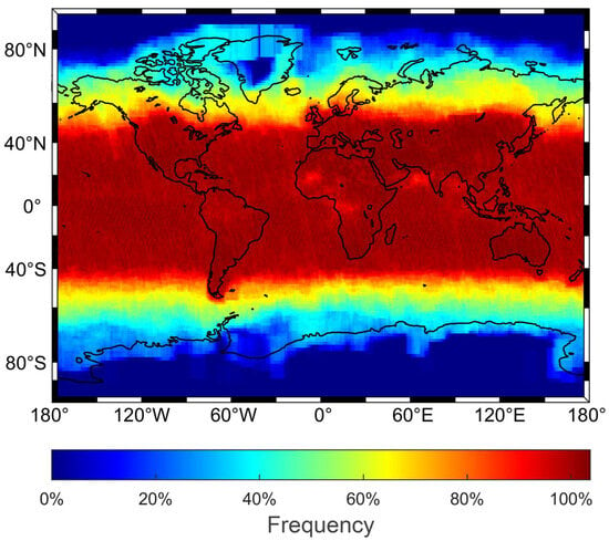
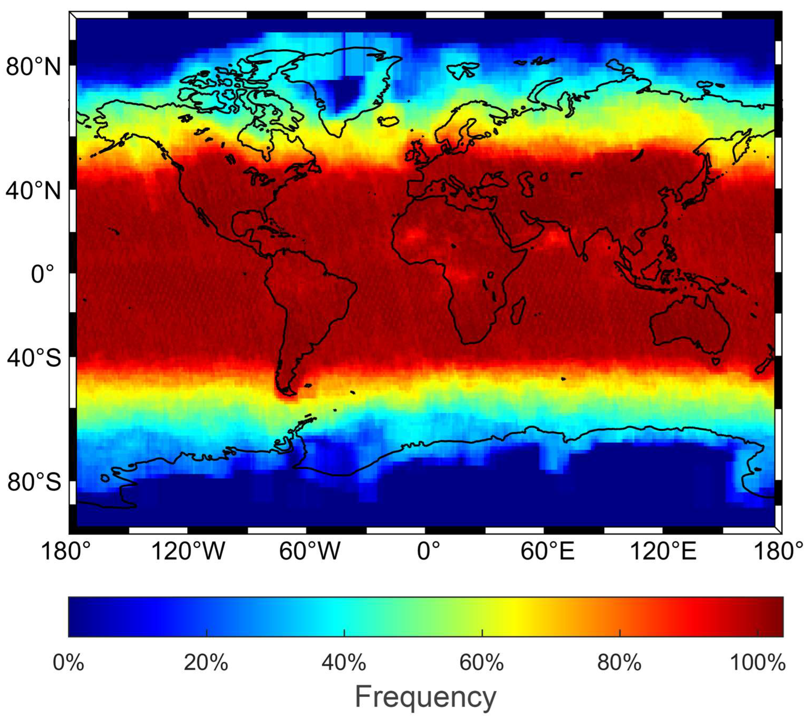
The NASA satellite OCO-2, designed to collect global measurements with sufficient precision, coverage, and resolution to help tackle regional-scale sources and sinks of CO2, was launched on 2 July 2014 [18]. Sampling at about 1:30 p.m. local time, OCO-2 operates in a sun-synchronous orbit and provides detailed descriptions of its ground-track repeat cycle (~16 days) [37]. We used the dataset NASA OCO-2 Level 2 Full-Physics Bias-Corrected XCO2 Daily Aggregated Product (V11, DOI: 10.5067/70K2B2W8MNGY), derived from these spectra using a physics-based retrieval method [38]. Across multiple validation studies, OCO-2 XCO2 retrievals agree well with ground-based TCCON measurements, exhibiting small biases (e.g., globally aggregated bias ≤ 0.20 ppm in v11.1 data with −0.03 ± 0.85 ppm in land nadir/glint) and high correlation (r ≈ 0.91), with typical RMSE values in the order of ~0.8–1.5 ppm, highlighting the robust consistency between satellite and TCCON observations [25,39,40,41,42]. The original product has a spatial resolution of 2.25 km × 1.29 km with quality flags. After removing low-quality data using observation quality flags, we gridded the raw OCO-2 along-track measurements into monthly 1° × 1° averages (the detailed processing procedure is provided in the Supplementary Material), then filled data gaps in sparsely populated grids through spatial interpolation where at least neighboring grids contained valid observations. Then, we obtained a monthly average XCO2 with spatial resolution of 1° from January 2015 to December 2020. However, due to the constraints of the sun-synchronous orbit and retrieval quality, data gaps exist in high-latitude regions above 65° (Figure 1).
Figure 1.
Sample frequency distribution of XCO2 observations during 2015 to 2020. The color represents the total for months that data are available.
2.2. CarbonTracker2019
The CarbonTracker2019 model is an inverse model that provides global atmospheric CO2 estimates with 2° latitude 3° longitude spatial resolution by the global TM5 model [43,44]. The model incorporates in situ measurements of atmospheric CO2 concentrations from the towers, aircraft air core [45], and surface measurement platforms distributed over 460 global stations. CarbonTracker resolves differences in spliced data resolutions by resampling all inputs to a common temporal framework before assimilation, ensuring consistent and comparable inversion results. For the CarbonTracker2019 considered in this analysis, we used the original CarbonTracker2019B version, released in May 2020 [44], but it was only updated to March 2019 (available at https://gml.noaa.gov/ccgg/carbontracker/CT2019B/download.php (accssed on 1 November 2025)). To expand the data to December 2020, we used the CarbonTracker near-real-time CT-NRT.v2022-1). The column-averaged XCO2 is derived from the CarbonTracker three-dimensional CO2 fields, thus representing a model-based product. The original product has a spatial resolution of 1° × 1° and is provided at a daily temporal frequency, and we aggregated into monthly averages.
2.3. Sea Surface pCO2
We used the monthly pCO2 fields with a 1° × 1° resolution generated by the CMEMS during 2015 to 2020 (available at https://data.marine.copernicus.eu/product/MULTIOBS_GLO_BIO_CARBON_SURFACE_MYNRT_015_008 (accessed on 13 September 2025)), which provides monthly reconstructions of key surface carbonate system variables, including surface ocean pCO2. The product is generated using a multi-observation neural-network approach trained on SOCAT in situ measurements and environmental predictors [46,47]. The predictors are chemical, biological, and physical variables commonly associated with variations in sea surface pCO2, including sea surface temperature, sea surface salinity, XCO2, sea surface height, mixed-layer depth, and chlorophyll a. An ensemble of 100 feedforward neural network models was used to reconstruct over the global surface ocean. This dataset shows good fitness with a mean bias close to zero, a root mean square error of 20.48 µatm, and a coefficient of determination of 0.76 at the global scale. The yearly bias drops during the following years and fluctuates around zero from 1994 onwards [46]. The original data are provided on a 0.25° × 0.25° grid and were bilinearly interpolated to a 1° × 1° regular grid to ensure consistency with other datasets and to facilitate regional analysis.
2.4. Regional Division
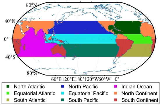
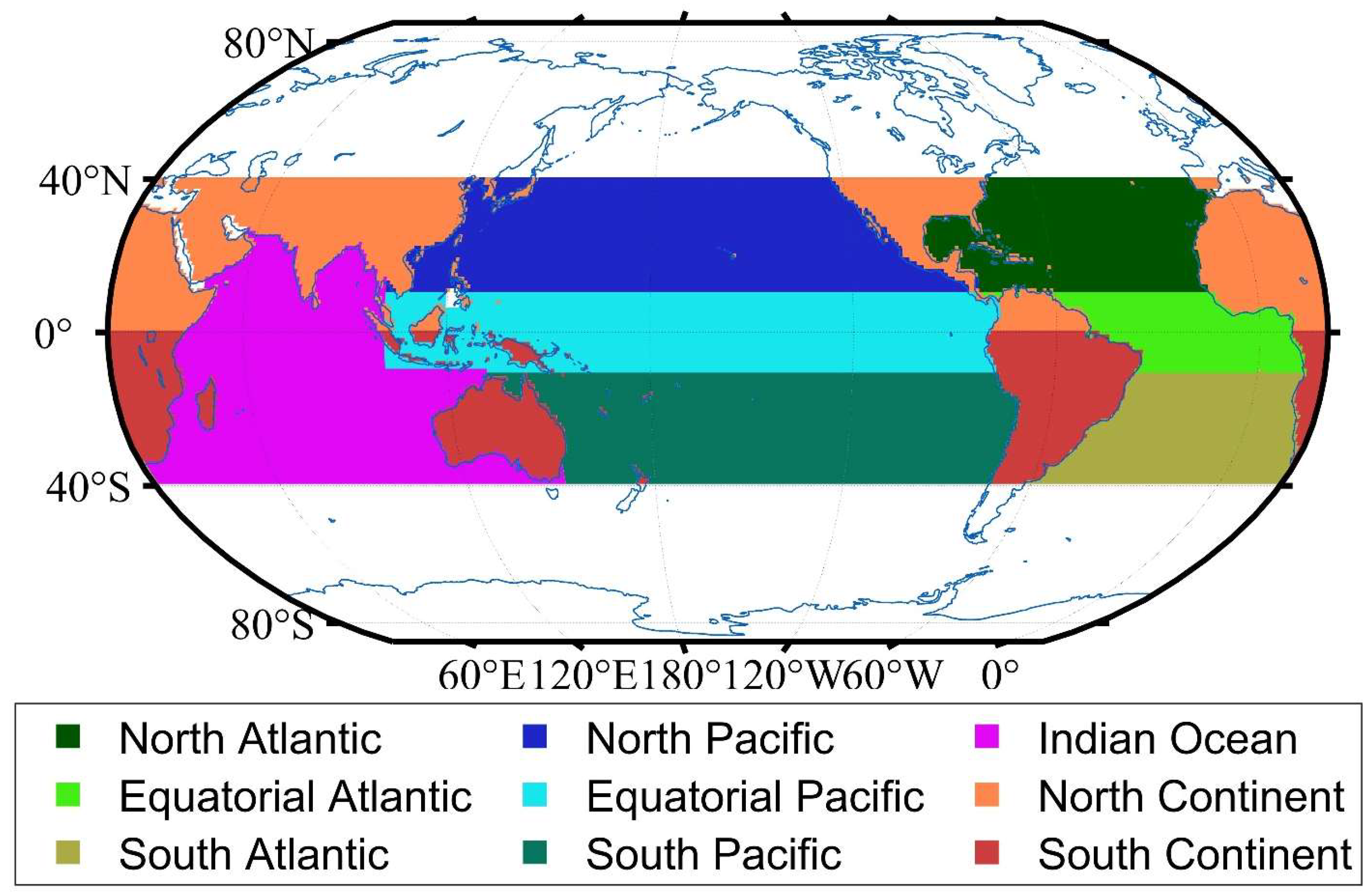
To analyze regional differences in variability in atmospheric and oceanic CO2 across low-latitude regions (40°S–40°N), the ocean was divided into seven geographical units. This segmentation is based on a simplified version of the Longhurst biogeographical provinces [48], which delineate oceanic regions according to physical forcing, biological structure, and biogeochemical regimes. The Longhurst system is defined based on physical–biological characteristics such as mixed-layer dynamics, nutrient regimes, and phytoplankton distributions, which are closely linked to air–sea CO2 exchange and surface ocean carbon variability. The Longhurst system comprises over 50 provinces, but for the purpose of large-scale carbon flux analysis, we aggregated adjacent provinces with similar climatic and oceanographic characteristics into broader, statistically robust regions, as shown in Figure 2.
Figure 2.
Location of the 9 regions. Colors are used solely to distinguish between regions. The regions include North Atlantic, Equatorial Atlantic, South Atlantic, North Pacific, Equatorial Pacific, South Pacific, Indian Ocean, North Continent, and South Continent.
2.5. Deseasonalization and Estimation of Mean Trends
To quantify the long-term increase and suppress short-term seasonal variability, we first applied a deseasonalization procedure to the monthly time series. For each grid cell, the monthly climatological mean was calculated based on the full study period (e.g., 2015–2020), representing the mean seasonal cycle. These climatological values were then subtracted from the corresponding monthly observations to produce deseasonalized residuals, which retain interannual and long-term signals while minimizing seasonal influences from biospheric activity and atmospheric transport. Thus, we performed regression analysis using the deseasonalized data to quantify long-term trends over the time series.
The six-year mean trend was subsequently estimated by performing an ordinary least squares linear regression on the deseasonalized monthly XCO2 data over time. The slope of the fitted line, expressed per year, represents the average annual increase over the study period. Additionally, for high-latitude grid cells lacking winter data, our deseasonalization procedure primarily targets seasonal cycles in spring, summer, and autumn. The resulting six-year mean trends derive from these seasons, with only statistically significant increasing trends (p < 0.05) retained after rigorous filtering. This approach is consistent with established methods used in trend detection and enables spatial comparison of growth patterns across different regions.
3. Results
3.1. Seasonal Variation in XCO2
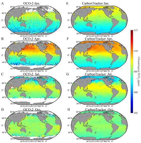
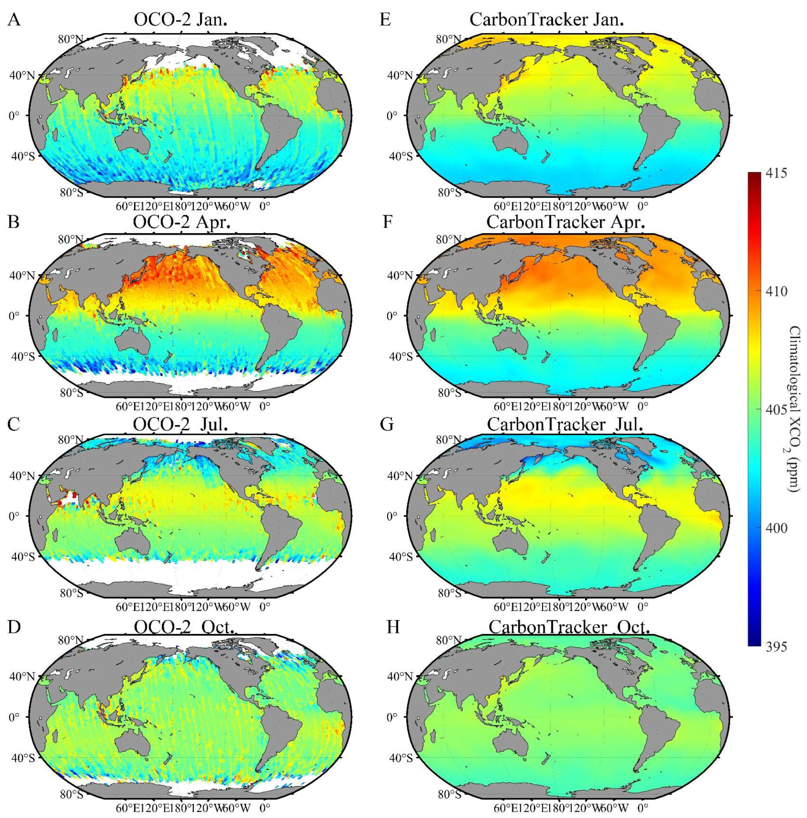
Figure 3 shows the spatial distribution of the seasonal XCO2 from OCO-2 observation and CarbonTracker2019 modeling during 2015 to 2020. There is good agreement in XCO2 seasonal variation estimated by modeling and observed by OCO-2, especially over the Northern Hemisphere, with high XCO2 exhibited in April. However, the model overestimates the XCO2 in January (approximately 2~3 ppm) in the Northern Hemisphere. The larger discrepancies between OCO-2 and CarbonTracker in winter and spring likely reflect OCO-2’s stronger sensitivity to enhanced atmospheric transport and seasonally intensified ocean carbon uptake, which are partially smoothed in inversion-based products [49]. Based on previous validation studies, satellite and model XCO2 products complement each other and emphasize the importance of region-specific error assessment frameworks for data assimilation and climate applications [50,51,52]. Overall, from both the OCO-2 observation and CarbonTracker2019 modeling, we can see the significant seasonal variations in XCO2 in both hemispheres, especially in the Northern Hemisphere. A previous study found that CarbonTracker2013 failed to estimate the seasonal variation amplitude in the high-latitude region (46°N–53°N) of both the Northern Hemisphere and the Southern Hemisphere [50]. However, in our study, we observed that the seasonal variation amplitude in the Southern Hemisphere was improved in CarbonTracker2019 when compared to OCO-2 observations. This improvement contributes to a more accurate representation of the spatial distribution of XCO2. Therefore, for XCO2 during 2010–2014, which cannot be measured by OCO-2, we also took CarbonTracker2019 as an auxiliary instrument in this study.
Figure 3.
Spatial distribution of the seasonal mean XCO2 (with unit of ppm) over 2015–2020 observed by OCO-2.
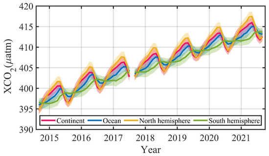
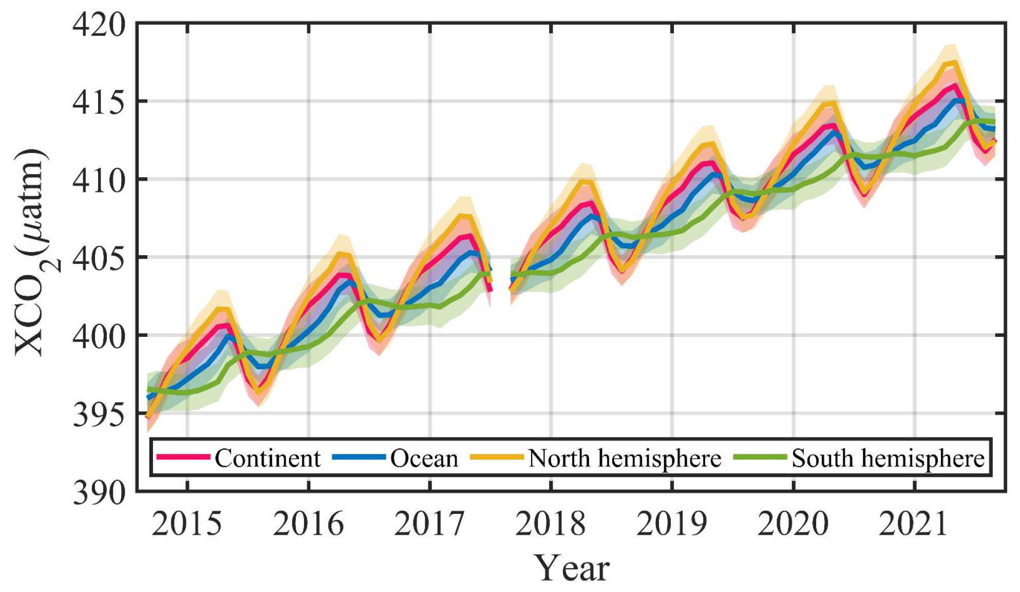
In addition, we calculated the temporal mean values for different regions, as shown in Figure 4. The average standard deviations are 0.76 ppm for continent, 0.60 ppm for ocean, 0.57 ppm for the Northern Hemisphere, and 0.39 ppm for the Southern Hemisphere. The coefficient of variation across these regions ranges between 0.29% and 0.56%. There are quite different seasonal variations in XCO2 from OCO-2 observations in the Northern Hemisphere and the Southern Hemisphere (Figure 4). The XCO2 exhibits larger seasonal variation amplitudes in the Northern Hemisphere than in the Southern Hemisphere, consistent with the results reported by a previous study [53], which still represent the dominant seasonal cycles in 2015–2020. The XCO2 in the Northern Hemisphere increases from September to the following April and decreases from May to August. However, in the Southern Hemisphere, XCO2 increases from February to July and decreases from August to the following January. Moreover, we found that the magnitude of the annual amplitude in the Northern Hemisphere (5.67 ± 0.42 ppm) is more than four times larger than in the Southern Hemisphere (1.2 ± 0.18 ppm). Previous investigation also showed that the magnitude of seasonal variability in XCO2 was much smaller in the Southern Hemisphere than the Northern Hemisphere [54]. These discrepancies in seasonal variation magnitudes result in higher seasonal XCO2 gap between the two hemispheres. Besides the difference in seasonal variation between the two hemispheres, there are also some differences in the XCO2 seasonal variation between land and ocean. We can clearly see that the seasonal variation in the ocean has a one-month delay after the variation in the land, which is likely due to differences in the seasonal cycles of air–sea and land CO2 fluxes, as well as the influence of prevailing westerly winds and subsequent atmospheric adjustment processes [55,56,57,58], yielding a total transport and mixing timescale of ~3–5 weeks. Second, the magnitude of the seasonal variation in XCO2 in the land is about 1.5 ppm larger than in the ocean. Due to the strong buffering capacity of marine carbonate systems [59] and the out-of-phase seasonal variability of thermal and non-thermal drivers of sea surface pCO2, oceanic CO2 fluxes exhibit relatively weak seasonality.
Figure 4.
Long-term monthly mean XCO2 from OCO-2 observations from the continent (red), ocean (blue), Northern Hemisphere (yellow), and Southern Hemisphere (green). All curves represent monthly averaged values, and the shaded areas indicate the associated uncertainties.
3.2. Seasonal Variation in Sea Surface pCO2
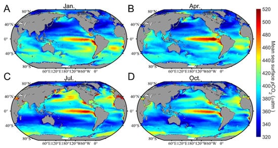
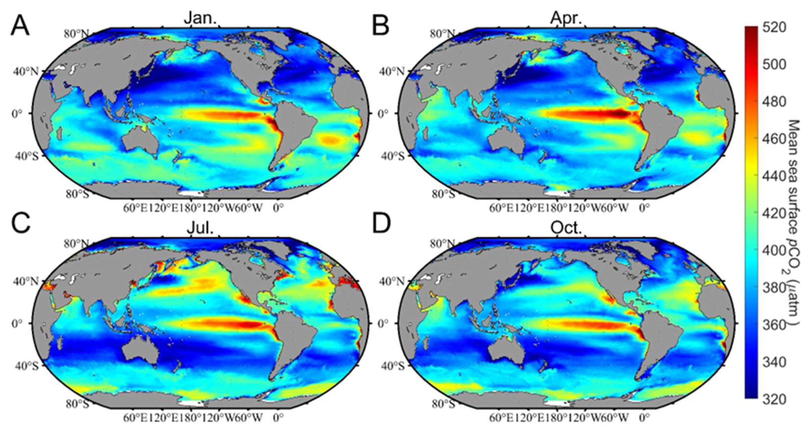
We similarly plotted the seasonal distribution of the climatological sea surface pCO2 for 2015–2020 generated by CMEMS (Figure 5). The spatial distribution of sea surface pCO2 is more complex compared to the atmosphere. Atmospheric CO2 usually shows a simple latitudinal variation; however, sea surface pCO2 exhibits a restricted east–west variation at the same latitude. Global ocean pCO2 varies greatly (over 200 μatm), with maximum values occurring in the equatorial Pacific and minimum values occurring in the midlatitudes. High sea surface pCO2 values (>500 µatm) are mainly observed in the eastern equatorial Pacific and Atlantic, where persistent wind-driven upwelling supplies carbon-rich subsurface waters to the surface, and are further enhanced by reduced CO2 solubility under high sea surface temperatures [9,60]. The summer maximum of sea surface pCO2 in the North Pacific is largely controlled by thermal effects and seasonal mixed-layer shoaling, which dominate over biological CO2 uptake after the spring bloom [9,61,62]. High values of pCO2, close or even higher than atmospheric levels, are found around tropics, which were deemed CO2 sources in previous studies [63,64,65]. The northern midlatitudes generally have very low pCO2 values, usually lower than 380 µatm, with clearly higher values in the east, and a similar pattern can be found in the South Pacific. The Arctic acts as a vital sink, with low pCO2 values in the 325–360 µatm range.
Figure 5.
Spatial distribution of seasonal mean sea surface pCO2 (with unit of μatm) over 2015–2018 generated by CMEMS.
As for seasonal variation, in most middle and low latitudes, the highest pCO2 values are observed during the warmest months and lowest in the coldest months. This seasonal trend is particularly pronounced in the Mediterranean Sea and Eastern Pacific Ocean, where the seasonal pCO2 amplitude can reach 70 µatm. Long-term increases in seasonal pCO2 amplitudes, especially in subtropical and Southern Ocean regions, have been linked to the continued uptake of anthropogenic CO2 [66]. However, in subarctic regions, the highest pCO2 is found in the winter, such as in the Bering Sea and Baltic Sea. Long-term increases in seasonal pCO2 amplitudes, especially in subtropical and Southern Ocean regions, have been linked to the continued uptake of anthropogenic CO2 [66]. In addition, although the Arctic plays a vital part as a global ocean sink (approximately 60%), high pCO2 values have been observed in coastal waters, especially in the east Siberian shelves [64,67]. This high pCO2 could be highly influenced by the discharge of highly oversaturated riverine waters. The open ocean at low and midlatitudes in the Northern Hemisphere exhibits high summer (July) and low winter (January), and this seasonal variation is more pronounced in marginal seas that are closely associated with human activities, such as the Gulf of St. Lawrence and the Persian Gulf. The marginal seas, on the other hand, usually have higher pCO2 than the adjacent oceans (e.g., the coastal Chilean and the Okhotsk Sea). In this basin north of the Equator, April, May, and June are the months with the highest pCO2, and the seasonal variations do not exceed 30 µatm. In contrast, the seasonal cycle is quite pronounced in the Indian Ocean south of the Equator (∼50 µatm).
3.3. Long-Term Changes in the Air–Sea Carbon Cycle
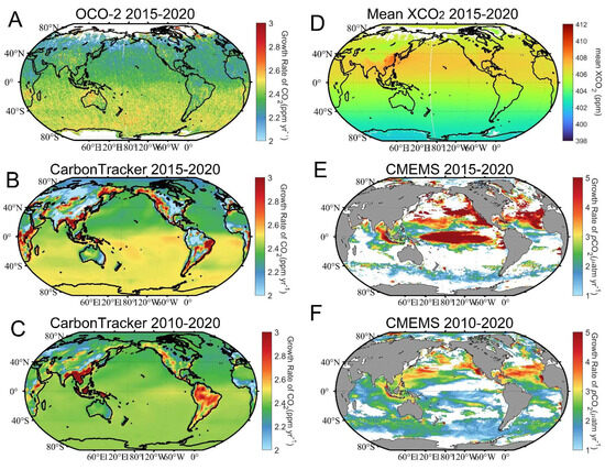
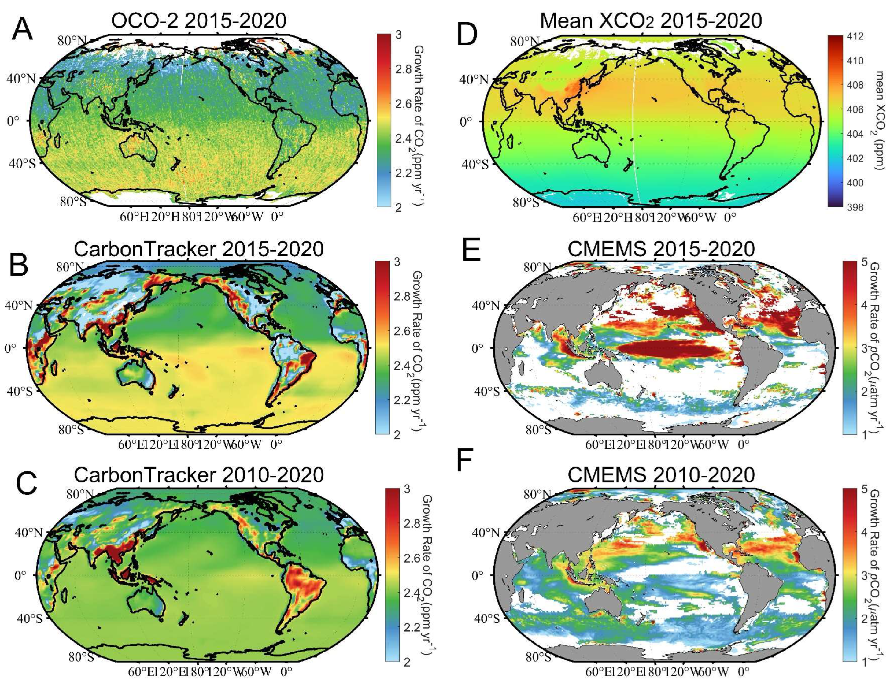
Figure 6 shows the mean 6-year trend of the atmospheric XCO2 and sea surface pCO2. The increasing rate from CarbonTracker2019 is significant in continental regions, for example, the North Pacific coastal region and Southeast Asia, while this result is not evident based on satellite XCO2. In addition, during 2015–2020, the XCO2 consistently increased from 398.85 ± 2.28 ppm to 415.97 ± 2.26 ppm by global average. However, the mean annual increasing trend is slightly different between the two hemispheres during 2015 to 2020. The XCO2 from OCO-2 and CarbonTracker2019 both exhibit a slightly lower six-year mean trend in the Northern Hemisphere (2.39 ppm yr−1) compared to the Southern Hemisphere (2.48 ppm yr−1) (Figure 6A,B). In addition, since the OCO-2 monthly average results are generated by gridding the data along the orbit, there are some spots in the gridded results due to the intra-month variation. However, this hemispheric difference disappears when we calculate the CO2 growth rate for 2010–2020 in the same way (Figure 6C). Therefore, we speculate that after the record 2009–2010 increase between hemispheres [68], the north–south atmospheric difference decreased in 2015–2020. This decline may have come from the increase in the carbon sink of the Northern Hemisphere terrestrial ecosystem, the continued increased uptake in the Southern Hemisphere Ocean [69], and the spontaneous cross-hemispheric transport of CO2 caused by the difference in the north–south gradient (Figure 6D). While Figure 6D illustrates the general pattern of the north–south gradient and associated transport, we recognize that it alone does not fully capture the complexity of these dynamics. Annual variability is quite different in the oceans, with the most noticeable increases in 2015–2020 occurring in equatorial regions and the Northern Hemisphere midlatitude regions (larger than 5 μatm yr−1), with other regions typically showing moderate increases (2~3 μatm yr−1) or no significant changes over this period (Figure 6E). This may be related to the exceptionally strong El Niño event in 2016. Additionally, it is noteworthy that the 6-year trend may be sensitive to interannual variability, and the selection of starting years could introduce biases to the study. Throughout 2010–2020, sea surface pCO2 shows a clear upward trend, with the Northern Hemisphere (approximately 2.4 μatm yr−1) rising at a significantly higher rate than the Southern Hemisphere (approximately 1.8 μatm yr−1), and the maximum rate of increase occurs in the 30–40 latitude band of the Northern Hemisphere. The fastest pCO2 growth rates occur in the North Atlantic, likely driven by warming-induced reduced CO2 solubility and increased Revelle factor values, while the Southern Ocean shows comparatively weaker growth because Ekman upwelling brings old, low-anthropogenic-CO2 waters to the surface and strong winds enhance mixing, diluting the anthropogenic signal. An enhanced period of the Southern Ocean carbon sink occurs after 2000, which is a determinant of the variations in the global ocean carbon sink [69,70,71]. Additionally, previous results demonstrate that even within the Northern Hemisphere atmosphere, Southern Hemisphere ocean fluxes are the dominant source of variability in XCO2 [29]. Therefore, the explanation for the interhemispheric gradient variation may involve a trend in the Southern Hemisphere ocean CO2 uptake. We fully acknowledge that the relatively short period analyzed (2015–2020) may be affected by decadal-scale variability. We regard this as an important caveat of our current study and intend to assess such longer-term influences when more extended satellite time series become available.
Figure 6.
Spatial distribution of the growth rate for XCO2 (with unit of ppm yr−1) during 2015–2020 generated by (A) OCO-2 and (B) CarbonTracker2019, and (C) the growth rate during 2010–2020 generated by CarbonTracker2019. (D) Climatology-averaged XCO2 during 20152020 generated by OCO-2. Spatial distribution of the growth rate for surface pCO2 (with unit of μatm yr−1) generated by CMEMS during (E) 2015–2020 and (F) 2010–2020. Grid cells with p > 0.01 are left blank.
4. Discussion
4.1. Variation Changes in the Regional Sectors
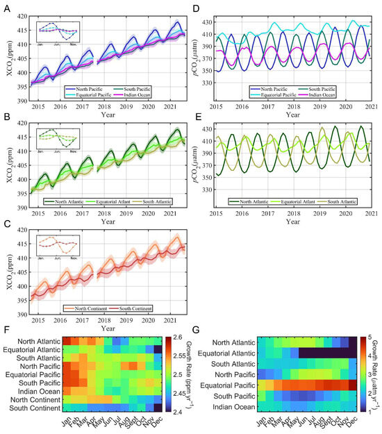
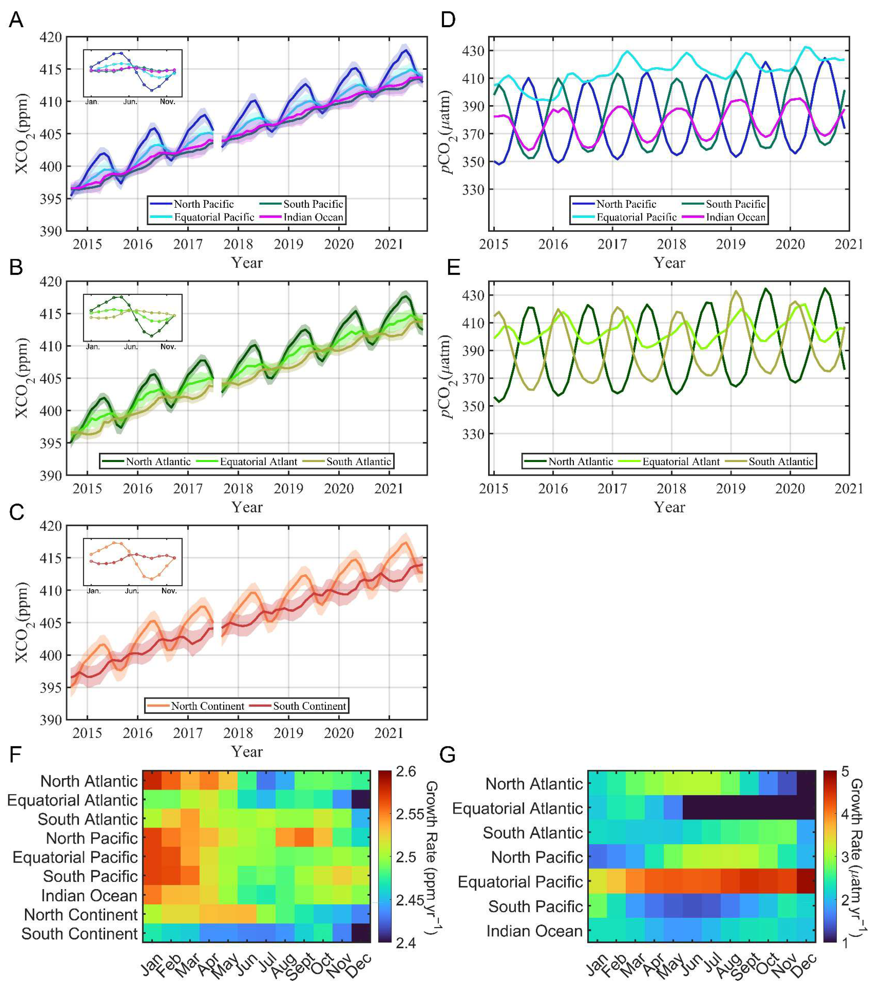
To gain a better understanding of the temporal variation in different regions, we divided the area between 40°S and 40°N into 9 regions based on geographical location and latitude: North Atlantic, Equatorial Atlantic, South Atlantic, North Pacific, equatorial Pacific, South Pacific, Indian Ocean, North Continent, and South Continent. Although east–west gradients exist—especially in the equatorial Pacific due to upwelling—the zonal variability is secondary to the dominant seasonal signal in our study context. Therefore, our regional partitioning primarily considers the influence of different latitudinal zones. We calculated the monthly atmospheric CO2 concentration (Figure 7A–C) and sea surface pCO2 (Figure 7D,E) in the corresponding regions from 2015 to 2020. In general, the atmospheric CO2 concentration increases in a steady trend in all nine regions (Table 1), with the fastest growth rate in the South Pacific and South Atlantic regions. The average standard deviations across these regions range between 0.79 ppm and 1.58 ppm.
Figure 7.
Temporal variation in XCO2 in different regions: (A) Pacific Ocean and Indian Ocean, (B) Atlantic Ocean, and (C) continent. Temporal variation in sea surface pCO2 in different regions: (D) Pacific Ocean and Indian Ocean and (E) Atlantic Ocean. Mean regional growth rate for (F) XCO2 and (G) sea surface pCO2.
Table 1.
Growth rate (ppm yr−1) (all p-value < 0.01) and seasonal variation (ppm) in different regions. The seasonal variability algorithm is detailed in the Supplementary Information.
The difference in growth rates between the Northern Hemisphere and Southern Hemisphere is more pronounced in the oceans than in the continents, while the Atlantic Ocean is the ocean with the most pronounced north–south difference.
To remove the effect of the long-term changing trend, we divide the XCO2 variability into long-term trend and net seasonal amplitude (the upper-right panel of Figure 7F,G). The regional variations indicate more details of the seasonal fluctuation in that those of the Indian Ocean are more consistent with the Southern Hemisphere, exhibiting a nonsignificant seasonal amplitude and a slight peak in June. However, the equatorial Pacific and Atlantic are more like the seasonal cycle in the Northern Hemisphere, reaching a net seasonal peak in May and a bottom in August. Moreover, unlike all other regions, the Southern shows two peaks of XCO2 in June and October during the year. If the decrease in February–March comes from the uptake of CO2 by the terrestrial ecosystem during the summer’s high productivity, the other decrease in August may indicate the uptake of seawater during the winter. This ocean sink can also be reconfirmed in the variability in XCO2 over the Southern Atlantic Ocean and Southern Pacific Ocean in October. This may imply that with horizontal diffusion and atmospheric circulation, there is also a significant effect on XCO2 over land due to oceanic uptake in the Southern Hemisphere winter.
To further explain these seasonal patterns, we compared the seasonal cycle of XCO2/pCO2 with marine biological activity using MODIS-derived chlorophyll a as a proxy for primary productivity [72,73]. In regions with strong seasonal phytoplankton blooms (e.g., North Atlantic and North Pacific), chlorophyll-a peaks during spring–summer coincide with pronounced pCO2 reductions, supporting the role of biological CO2 uptake in driving seasonal pCO2 variability. In contrast, equatorial regions show weaker seasonal chlorophyll variations and a more complex pCO2 pattern dominated by upwelling and physical mixing, which weakens the biological control.
The mean 6-year trend of CO2 in the two hemispheres is completely different in seawater and in the atmosphere. Although the atmospheric rate of increase differs in different regions, both the whole atmospheric CO2 concentrates show greater variability from January to March. Although this difference is less than 0.2 ppm yr−1 (approximately one-tenth of the trend), the long-term persistence of this trend will lead to larger seasonal variability between the two hemispheres. At the same time, this seasonal difference in growth rate is not found for sea surface pCO2, which shows much larger variability with unclear trends. This is probably due to the fact that the period of this study (2015 to 2020) is not sufficient to capture the correct pattern of pCO2 growth in different months, and we will conduct an extended study when more data are available.
4.2. Variation Changes for the Coastal Oceans
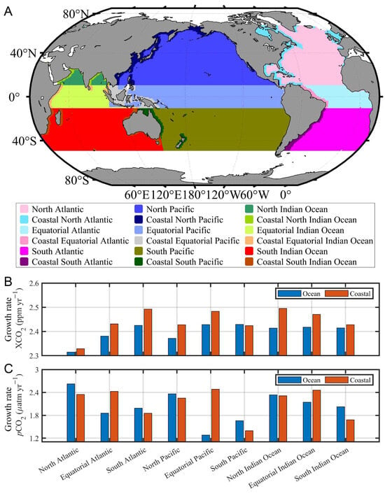
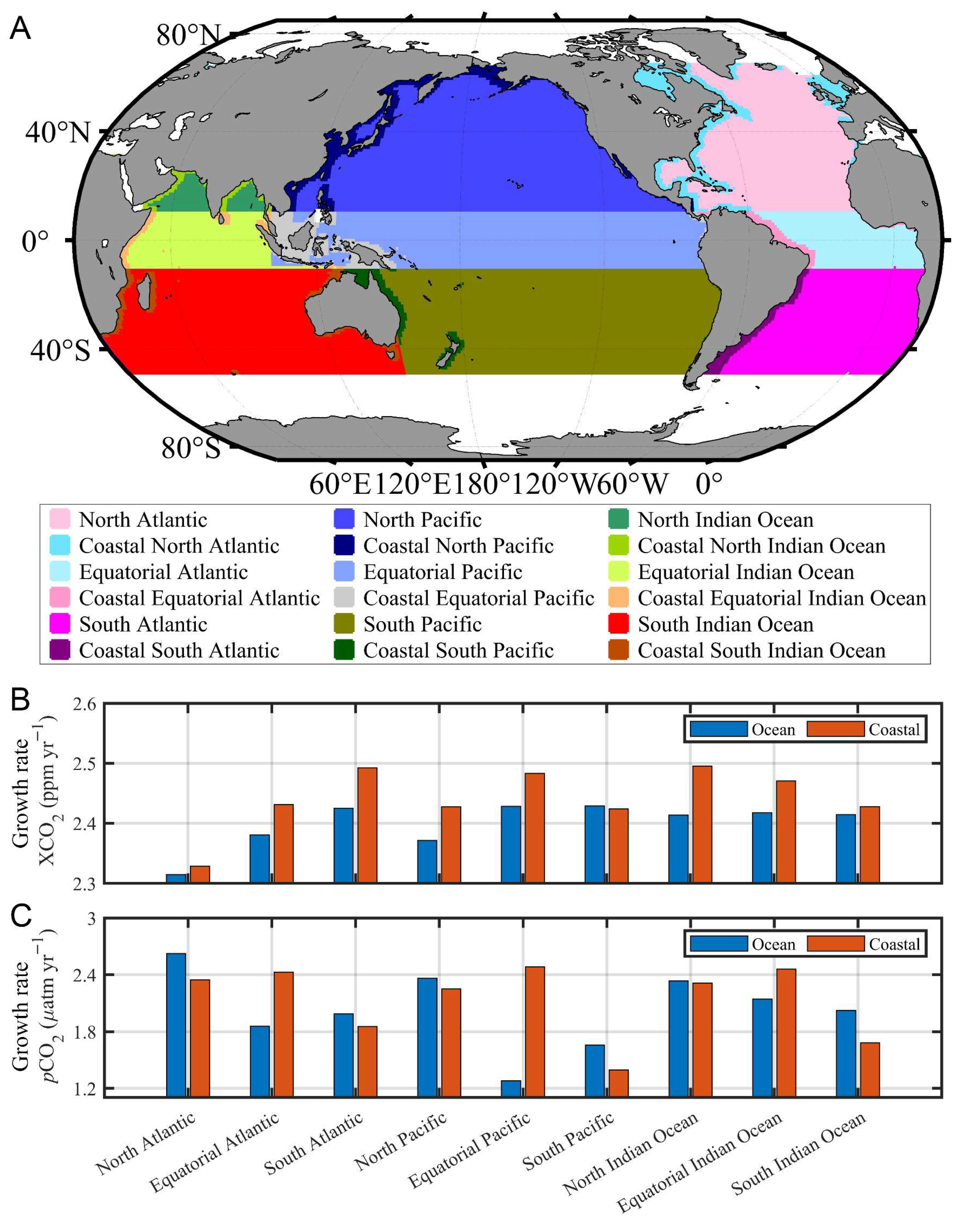
In our study, we found more detailed distinctions after further analyzing the nearshore and open ocean individually. The atmospheric XCO2 is rising significantly more rapidly in marginal and coastal regions than open oceans at the same latitude. In contrast, sea surface pCO2 midlatitude coastal waters show similar or lower growth rates than open oceans at the same latitude. Thus, we hypothesize that anthropogenic emissions cause rapidly increasing atmospheric CO2, resulting in a CO2 growth rate that is more significant over marginal sea, which is closer to land. Due to the stronger biological effect and buffering capacity of marginal sea—characterized by enhanced primary productivity and higher total alkalinity that stabilize seawater pCO2—a large fraction of the CO2 sinks at marginal sea [74,75,76,77]. However, in the equatorial region (including the Atlantic, Pacific, and Indian Oceans), sea surface pCO2 in open oceans exhibits faster growth rates than coastal waters (Figure 8C). The faster open-ocean pCO2 increase reflects ENSO-driven upwelling and warming, whereas coastal waters were mitigated by higher biological uptake and stronger mixing/terrestrial influences.
Figure 8.
(A) Location of marginal seas and open oceans (divided by the 200 m isobath). Long time-series growth rates of regional atmospheric XCO2 (B) and sea surface pCO2 (C) in the open ocean and marginal seas (including nearshore waters) during 2015 to 2020.
Another interesting finding is that during 2015 to 2020, seawater pCO2 increases significantly faster in all equatorial sea areas than in marginal sea areas at the same latitude. The most notable difference occurs in the equatorial Pacific, where the open ocean is higher by about 1.2 μatm yr−1 than the coastal. During strong El Niño events, the tropical Pacific Ocean also plays an important role, as it is the source of atmospheric CO2 and equatorial upwelling brings CO2-rich water from the inner ocean to the surface [30]. This equatorial upwelling in the eastern and central Pacific is suppressed, reducing the supply of CO2 to the surface. The reduction in ocean-to-atmosphere CO2 fluxes should help slow the growth in atmospheric CO2.
4.3. Variation Changes for the Low-Latitude Southern Hemisphere Ocean
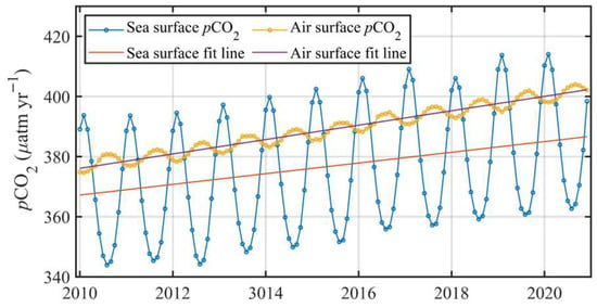
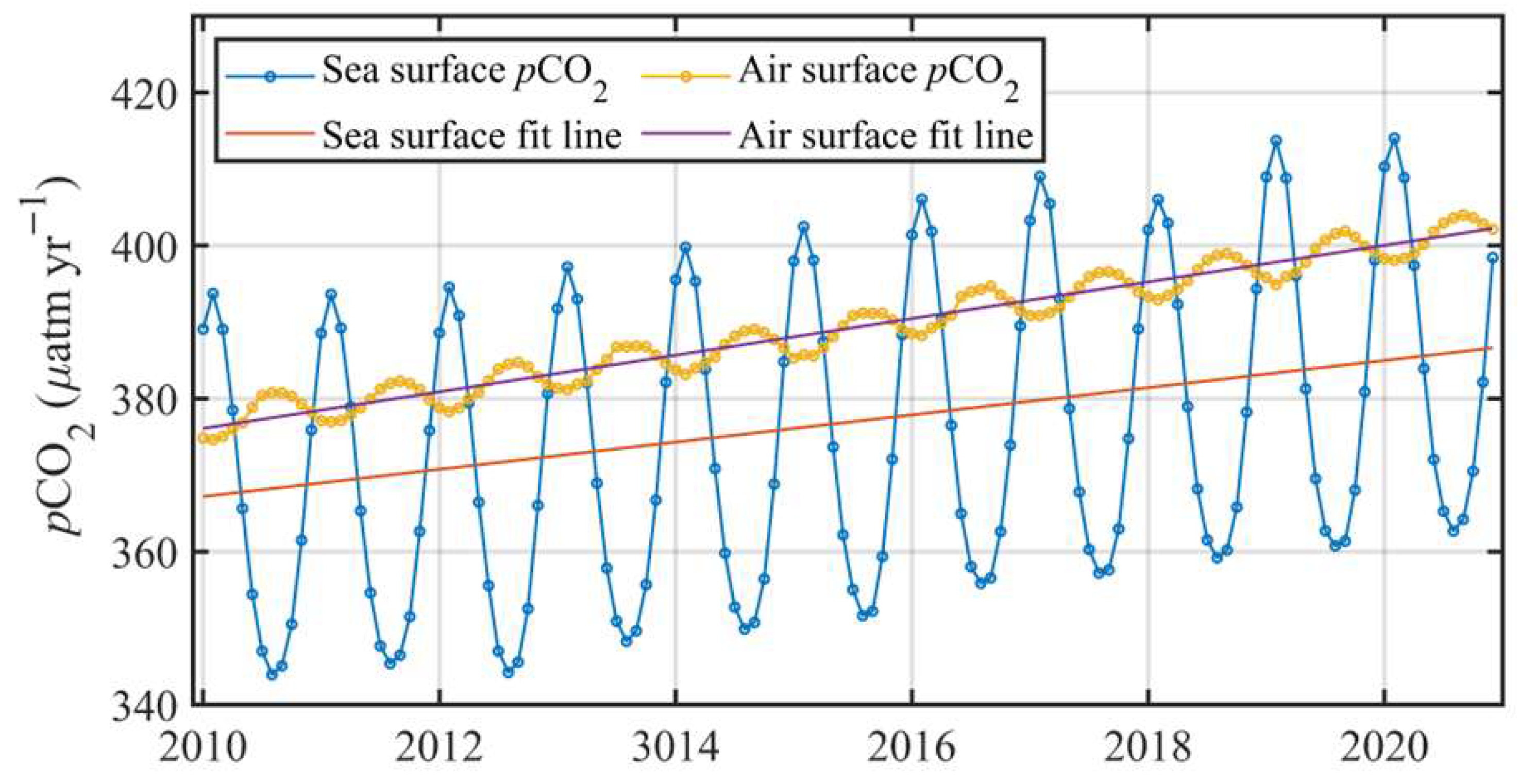
To better understand atmospheric control of the enhancement of the low-latitude Southern Hemisphere ocean CO2 sink, we compared the temporal evolution of sea surface pCO2 with the corresponding atmospheric pCO2 at latitudes of 10–40°S during 2010–2020 (Figure 9). Atmospheric pCO2 was converted from XCO2 and adjusted to saturated water vapor pressure using concurrent atmospheric pressure and sea surface temperature, ensuring consistency with the sea surface conditions.
Figure 9.
Monthly sea surface pCO2 of seawater and atmosphere at the low-latitude Southern Hemisphere ocean air–sea interface from 2010 to 2020.
Our results show that both atmospheric and oceanic pCO2 increased over the study period; however, the growth rate of atmospheric pCO2 exceeded that of sea surface pCO2. As a consequence, the air–sea pCO2 difference exhibited a persistent and monotonic increase, from 8.9 µatm in 2010 to 15.6 µatm in 2020. This widening gradient indicates a progressively stronger thermodynamic driving force for oceanic CO2 uptake (equivalent sea surface atmospheric pCO2 and error analysis are provided in the Supplementary Information).
The slower increase in sea surface pCO2 relative to the atmosphere suggests that oceanic buffering processes—such as physical mixing, air–sea gas exchange, and biological carbon uptake—partially dampened the atmospheric CO2 signal at the ocean surface. Under these conditions, the rapid rise in atmospheric CO2 acts as an external force that enhances the air–sea CO2 flux into the ocean, even in the absence of a corresponding acceleration in oceanic pCO2 growth. Therefore, the intensified low-latitude Southern Hemisphere CO2 sink during 2010–2020 can be primarily attributed to the increasing atmospheric CO2 burden rather than changes in oceanic carbon chemistry alone.
5. Conclusions
During the last few decades, global land and ocean carbon sinks have increased in proportion to the increase in CO2 emissions. Although we have gained a better understanding of atmospheric CO2 concentrations with the development of satellite technology, there are still few air–sea CO2 flux studies that focus on the effects of atmospheric changes on air–sea fluxes. Previous studies have often considered only the influence of sea surface pCO2 on sea–air carbon fluxes, while our analysis highlights the potential of atmospheric XCO2 observations to complement oceanic CO2 trend assessments.
This study leverages high-resolution satellite observations from OCO-2 and CMEMS to unravel the spatiotemporal heterogeneity of atmospheric XCO2 and sea surface pCO2 between 2015 and 2020. By integrating OCO-2 XCO2 with CMEMS pCO2 products, we demonstrate the potential of satellite remote sensing to characterize the spatiotemporal variability of CO2 in the atmosphere–ocean interface. Our approach overcomes traditional limitations of sparse in situ data, enabling robust analysis of seasonal and long-term trends on a global scale. We validate the possibility of using OCO-2 remote sensing data for time-series studies, and the high spatial resolution of atmospheric CO2 data provides an opportunity for us to ascend into the understanding of CO2 changes. We found that there are significant seasonal variations in the distribution of both atmospheric XCO2 and seawater. Atmospheric XCO2 has a clear latitudinal distribution with seasonal variation that mainly occurs in the Northern Hemisphere, and the magnitude of the annual amplitude in the Northern Hemisphere (5.67 ± 0.42 ppm) is more than four times that of the Southern Hemisphere (1.2 ± 0.18 ppm). Moreover, the misaligned CO2 peaks between the Northern and Southern Hemisphere promote the hemispheric movement of CO2, causing CO2 to be transported from the Northern Hemisphere to the Southern Hemisphere in summer.
We also analyzed the growth rate of CO2 in the atmosphere and at surface seawater, which indicated that the mean long-term trend of CO2 in the two hemispheres is completely different in seawater and in the atmosphere. Atmospheric CO2 concentrations show greater variability from January to March, which causes larger seasonal fluctuations. Additionally, the Southern Continent shows two seasonal peaks of XCO2, occurring in June and October. The June peak likely corresponds to increased uptake by terrestrial ecosystems during the high-productivity austral summer, while the October peak may reflect enhanced CO2 uptake by the adjacent ocean during the austral winter. In addition, coastal atmospheric CO2 concentrations tend to be higher than in the open ocean, but sea surface pCO2 tends to increase at a slightly lower rate than in the open ocean, indicating that marginal seas act as a better transition zone, taking up atmospheric CO2 from terrestrial sources without a rapid rise in sea surface pCO2. It is worth considering how the continued rise in atmospheric CO2 has an impact on oceanic uptake.
The launch of next-generation CO2 monitoring satellites (e.g., TANSAT-2, GOSAT-GW) will further enhance our ability to track anthropogenic and natural carbon fluxes. In addition, with the advancement of various observational techniques, eliminating systematic biases among different data sources and constructing a long-term, consistent, and continuous XCO2 dataset will facilitate a clearer understanding of air–sea CO2 exchange. Greater use of multi-satellite synergy is recommended to better capture ocean–atmosphere interactions, particularly during climate anomalies such as El Niño. While this study did not include in-depth calculations of air–sea carbon fluxes, future work will focus on more quantitative assessments. In terms of strengths and limitations, our study benefits from the long-term, high-resolution satellite datasets that provide broad spatial coverage and enable the analysis of both seasonal dynamics and long-term trends. However, one limitation is the uncertainties associated with XCO2 retrievals, such as those introduced by clouds, aerosols, or surface reflectance. The average standard deviations for hemispheric regions range between 0.39 ppm and 0.67 ppm (coefficient of variation ranges between 0.29% and 0.56%). Although OCO-2 data products include bias correction and quality filtering and are validated against in situ measurements, the confidence bounds of aggregated XCO2 averages remain an area for future improvement. In addition, extending the research to the current period represents a valuable direction and will be prioritized in our future studies.
Supplementary Materials
The following supporting information can be downloaded at: https://www.mdpi.com/article/10.3390/rs18040630/s1. References [78,79] are cited in the supplementary materials.
Author Contributions
Conceptualization, P.C.; writing—original draft, S.Z.; writing—review and editing, P.C., Z.Z., H.H., and D.P. All authors have read and agreed to the published version of the manuscript.
Funding
This research was funded by an Open Research Fund of Technology Innovation Center for South China Sea Remote Sensing, Surveying and Mapping Collaborative Application, Ministry of Natural Resources (RSSMCA-2024-B015), Open Research Fund of Bejing Institute of Space Mechanics & Electricity, China Academy of Space Technology (AIRSE202402), National Natural Science Foundation of China (4240060663; 42406176; 42322606; 42276180; 61991453), Special Fund for Basic Scientific Research, Second Institute of Oceanography, Ministry of Natural Resources (JG2025), Independent Research Fund of State Key Laboratory of State Key Laboratory of Satellite Ocean Environment Dynamics, Second Institute of Oceanography, Ministry of Natural Resources (SOEDZZ2528), Open Research Fund of State Key Laboratory of Physical Oceanography, Institute of Oceanographic Instrumentation, Qilu University of Technology (Shandong Academy of Sciences) (2025hyqzsKF01), China Postdoctoral Science Foundation (2023M740809), National Key Research and Development Program of China (2022YFB3901702; 2022YFB3901703; 2022YFB3902603), Key Special Project for Introduced Talents Team of Southern Marine Science and Engineering Guangdong Laboratory (GML2021GD0809), Key R&D Program of Shandong Province, China (2023ZLYS01), and Major Innovation Project of Science, Education and Industry Integration Pilot Project of Qilu University of Technology (Shandong Academy of Sciences) (2025ZDYS01).
Data Availability Statement
Dataset available on request from the authors. The raw data supporting the conclusions of this article will be made available by the authors on request.
Acknowledgments
We thank NOAA, CMEMS, and GML for providing valuable datasets, and we also thank SOCAT for collecting and processing the released carbonate products.
Conflicts of Interest
The authors declare no conflicts of interest. The funders had no role in the design of the study; in the collection, analyses, or interpretation of data; in the writing of the manuscript; or in the decision to publish the results.
Abbreviations
The following abbreviations are used in this manuscript.
| CO2 | carbon dioxide |
| OCO-2 | Orbiting Carbon Observatory 2 |
| CMEMS | Copernicus Marine Environment Monitoring Service |
| XCO2 | column-averaged CO2 |
| pCO2 | partial pressure of CO2 |
| NASA | National Aeronautics and Space Administration |
| GOSAT-2 | Greenhouse Gases Observing Satellite 2 |
| TCCON | Total Carbon Column Observing Network |
References
- Friedlingstein, P.; Jones, M.W.; O’Sullivan, M.; Andrew, R.M.; Bakker, D.C.; Hauck, J.; Le Quéré, C.; Peters, G.P.; Peters, W.; Pongratz, J. Global carbon budget 2021. Earth Syst. Sci. Data 2022, 14, 1917–2005. [Google Scholar] [CrossRef] [Scilit]
- Ballantyne, A.á.; Alden, C.á.; Miller, J.á.; Tans, P.á.; White, J. Increase in observed net carbon dioxide uptake by land and oceans during the past 50 years. Nature 2012, 488, 70–72. [Google Scholar] [CrossRef] [Scilit] [PubMed]
- McKinley, G.A.; Fay, A.R.; Lovenduski, N.S.; Pilcher, D.J. Natural variability and anthropogenic trends in the ocean carbon sink. Annu. Rev. Mar. Sci. 2017, 9, 125–150. [Google Scholar] [CrossRef] [Scilit]
- Peiro, H.; Crowell, S.; Schuh, A.; Baker, D.F.; O’Dell, C.; Jacobson, A.R.; Chevallier, F.; Liu, J.; Eldering, A.; Crisp, D. Four years of global carbon cycle observed from the Orbiting Carbon Observatory 2 (OCO-2) version 9 and in situ data and comparison to OCO-2 version 7. Atmos. Chem. Phys. 2022, 22, 1097–1130. [Google Scholar] [CrossRef] [Scilit]
- Weiss, R.F. Carbon dioxide in water and seawater: The solubility of a non-ideal gas. Mar. Chem. 1974, 2, 203–215. [Google Scholar] [CrossRef] [Scilit]
- Wanninkhof, R. Relationship between wind speed and gas exchange over the ocean revisited. Limnol. Oceanogr. Methods 2014, 12, 351–362. [Google Scholar] [CrossRef] [Scilit]
- Arroyo, M.C.; Fassbender, A.J.; Carter, B.R.; Edwards, C.A.; Fiechter, J.; Norgaard, A.; Feely, R.A. Dissimilar sensitivities of ocean acidification metrics to anthropogenic carbon accumulation in the Central North Pacific Ocean and California Current Large Marine Ecosystem. Geophys. Res. Lett. 2022, 49, e2022GL097835. [Google Scholar] [CrossRef] [Scilit]
- Schuster, U.; McKinley, G.A.; Bates, N.; Chevallier, F.; Doney, S.C.; Fay, A.R.; González-Dávila, M.; Gruber, N.; Jones, S.; Krijnen, J. An assessment of the Atlantic and Arctic sea–air CO 2 fluxes, 1990–2009. Biogeosciences 2013, 10, 607–627. [Google Scholar] [CrossRef] [Scilit]
- Takahashi, T.; Sutherland, S.C.; Wanninkhof, R.; Sweeney, C.; Feely, R.A.; Chipman, D.W.; Hales, B.; Friederich, G.; Chavez, F.; Sabine, C. Climatological mean and decadal change in surface ocean pCO2, and net sea–air CO2 flux over the global oceans. Deep Sea Res. Part II Top. Stud. Oceanogr. 2009, 56, 554–577. [Google Scholar] [CrossRef] [Scilit]
- Wanninkhof, R.; Park, G.-H.; Takahashi, T.; Sweeney, C.; Feely, R.; Nojiri, Y.; Gruber, N.; Doney, S.C.; McKinley, G.A.; Lenton, A. Global ocean carbon uptake: Magnitude, variability and trends. Biogeosciences 2013, 10, 1983–2000. [Google Scholar] [CrossRef] [Scilit]
- Bousquet, P.; Ciais, P.; Miller, J.; Dlugokencky, E.J.; Hauglustaine, D.; Prigent, C.; Van der Werf, G.; Peylin, P.; Brunke, E.-G.; Carouge, C. Contribution of anthropogenic and natural sources to atmospheric methane variability. Nature 2006, 443, 439. [Google Scholar] [CrossRef] [Scilit] [PubMed]
- Eldering, A.; Wennberg, P.O.; Viatte, C.; Frankenberg, C.; Roehl, C.M.; Wunch, D. The Orbiting Carbon Observatory-2: First 18 months of science data products. Atmos. Meas. Tech. 2017, 10, 549–563. [Google Scholar] [CrossRef] [Scilit]
- Buchwitz, M.; Schneising, O.; Burrows, J.; Bovensmann, H.; Reuter, M.; Notholt, J. First direct observation of the atmospheric CO 2 year-to-year increase from space. Atmos. Chem. Phys. 2007, 7, 4249–4256. [Google Scholar] [CrossRef] [Scilit]
- Bovensmann, H.; Burrows, J.; Buchwitz, M.; Frerick, J.; Noël, S.; Rozanov, V.; Chance, K.; Goede, A. SCIAMACHY: Mission objectives and measurement modes. J. Atmos. Sci. 1999, 56, 127–150. [Google Scholar] [CrossRef] [Scilit]
- Yokota, T.; Yoshida, Y.; Eguchi, N.; Ota, Y.; Tanaka, T.; Watanabe, H.; Maksyutov, S. Global concentrations of CO2 and CH4 retrieved from GOSAT: First preliminary results. Sola 2009, 5, 160–163. [Google Scholar] [CrossRef] [Scilit]
- Cogan, A.; Boesch, H.; Parker, R.; Feng, L.; Palmer, P.; Blavier, J.F.; Deutscher, N.M.; Macatangay, R.; Notholt, J.; Roehl, C. Atmospheric carbon dioxide retrieved from the Greenhouse gases Observing SATellite (GOSAT): Comparison with ground-based TCCON observations and GEOS-Chem model calculations. J. Geophys. Res. Atmos. 2012, 117. [Google Scholar] [CrossRef] [Scilit]
- Joiner, J.; Yoshida, Y.; Vasilkov, A.; Middleton, E. First observations of global and seasonal terrestrial chlorophyll fluorescence from space. Biogeosciences 2011, 8, 637–651. [Google Scholar] [CrossRef] [Scilit]
- Crisp, D. Measuring Atmospheric Carbon Dioxide from Space with the Orbiting Carbon Observatory-2 (OCO-2); SPIE: Bellingham, WA, USA, 2015; Volume 9607. [Google Scholar]
- Lei, R.; Feng, S.; Danjou, A.; Broquet, G.; Wu, D.; Lin, J.C.; O’Dell, C.W.; Lauvaux, T. Fossil fuel CO2 emissions over metropolitan areas from space: A multi-model analysis of OCO-2 data over Lahore, Pakistan. Remote Sens. Environ. 2021, 264, 112625. [Google Scholar] [CrossRef] [Scilit]
- Shekhar, A.; Chen, J.; Paetzold, J.C.; Dietrich, F.; Zhao, X.; Bhattacharjee, S.; Ruisinger, V.; Wofsy, S.C. Anthropogenic CO2 emissions assessment of Nile Delta using XCO2 and SIF data from OCO-2 satellite. Environ. Res. Lett. 2020, 15, 095010. [Google Scholar] [CrossRef] [Scilit]
- Hakkarainen, J.; Ialongo, I.; Tamminen, J. Direct space-based observations of anthropogenic CO2 emission areas from OCO-2. Geophys. Res. Lett. 2016, 43, 11400–11406. [Google Scholar] [CrossRef] [Scilit]
- Fu, P.; Xie, Y.; Moore, C.E.; Myint, S.W.; Bernacchi, C.J. A Comparative Analysis of Anthropogenic CO2 Emissions at City Level Using OCO-2 Observations: A Global Perspective. Earth’s Future 2019, 7, 1058–1070. [Google Scholar] [CrossRef] [Scilit]
- Liu, D.; Lei, L.; Guo, L.; Zeng, Z.-C. A Cluster of CO2 Change Characteristics with GOSAT Observations for Viewing the Spatial Pattern of CO2 Emission and Absorption. Atmosphere 2015, 6, 1695–1713. [Google Scholar] [CrossRef] [Scilit]
- Sheng, M.; Lei, L.; Zeng, Z.-C.; Rao, W.; Zhang, S. Detecting the Responses of CO2 Column Abundances to Anthropogenic Emissions from Satellite Observations of GOSAT and OCO-2. Remote Sens. 2021, 13, 3524. [Google Scholar] [CrossRef] [Scilit]
- Das, S.; Kiel, M.; Laughner, J.; Osterman, G.; O’Dell, C.W.; Taylor, T.E.; Fisher, B.; Chevallier, F.; Deutscher, N.M.; Dubey, M.K.; et al. Comparisons of the v11.1 Orbiting Carbon Observatory-2 (OCO-2) XCO2 Measurements With GGG2020 TCCON. Earth Space Sci. 2025, 12, e2024EA003935. [Google Scholar] [CrossRef] [Scilit]
- Deng, F.; Jones, D.B.; O’Dell, C.W.; Nassar, R.; Parazoo, N.C. Combining GOSAT XCO2 observations over land and ocean to improve regional CO2 flux estimates. J. Geophys. Res. Atmos. 2016, 121, 1896–1913. [Google Scholar] [CrossRef] [Scilit]
- Müller, A.; Tanimoto, H.; Sugita, T.; Machida, T.; Nakaoka, S.-i.; Patra, P.K.; Laughner, J.; Crisp, D. New approach to evaluate satellite derived XCO2 over oceans by integrating ship and aircraft observations. Atmos. Chem. Phys. 2021, 21, 8255–8271. [Google Scholar] [CrossRef] [Scilit]
- Liao, E.; Resplandy, L.; Liu, J.; Bowman, K.W. Amplification of the ocean carbon sink during El Niños: Role of poleward Ekman transport and influence on atmospheric CO2. Glob. Biogeochem. Cycles 2020, 34, e2020GB006574. [Google Scholar] [CrossRef] [Scilit]
- Guan, Y.; McKinley, G.A.; Fay, A.R.; Doney, S.C.; Keppel-Aleks, G. Ocean-driven interannual variability in atmospheric CO2 quantified using OCO-2 observations and atmospheric transport simulations. Front. Mar. Sci. 2024, 11, 1272415. [Google Scholar] [CrossRef] [Scilit]
- Chatterjee, A.; Gierach, M.; Sutton, A.; Feely, R.; Crisp, D.; Eldering, A.; Gunson, M.; O’Dell, C.; Stephens, B.; Schimel, D. Influence of El Niño on atmospheric CO2 over the tropical Pacific Ocean: Findings from NASA’s OCO-2 mission. Science 2017, 358, eaam5776. [Google Scholar] [CrossRef] [Scilit]
- Morozov, E.; Kondrik, D.; Chepikova, S.; Pozdnyakov, D. Atmospheric columnar CO2 enhancement over E. huxleyi blooms: Case studies in the North Atlantic and Arctic waters. Труды Карельскoгo научнoгo центра Рoссийскoй академии наук Transactions of the Karelian Research Centre of the Russian Academy of Sciences. 2019, 3, 28–33. [Google Scholar] [CrossRef] [Scilit]
- Ravi Kumar, K.; Prabir, K.P.; Kondapalli Niranjan, K.; Naveen, C.; Raju, A.; Rama Krishna, K. Spatio-temporal variability of XCO2 over Indian region inferred from Orbiting Carbon Observatory (OCO-2) satellite and Chemistry Transport Model. Atmos. Res. 2022, 269, 106044. [Google Scholar] [CrossRef] [Scilit]
- Crowell, S.; Baker, D.; Schuh, A.; Basu, S.; Jacobson, A.R.; Chevallier, F.; Liu, J.; Deng, F.; Feng, L.; McKain, K.; et al. The 2015–2016 carbon cycle as seen from OCO-2 and the global in situ network. Atmos. Chem. Phys. 2019, 19, 9797–9831. [Google Scholar] [CrossRef] [Scilit]
- Lim, Y.K.; Kovach, R.M.; Pawson, S.; Vernieres, G. The 2015/2016 El Niño Event in Context of the MERRA-2 Reanalysis: A Comparison of the Tropical Pacific with 1982/1983 and 1997/1998. J. Clim. 2017, 30, 4819–4842. [Google Scholar] [CrossRef] [Scilit]
- Chen, H.-C.; Tseng, Y.-H.; Huang, J.-H.; Juang, P.-H. Understanding the driving mechanisms behind triple-dip La Niñas: Insights from the prediction perspective. npj Clim. Atmos. Sci. 2025, 8, 143. [Google Scholar] [CrossRef] [Scilit]
- Gruber, N.; Clement, D.; Carter, B.R.; Feely, R.A.; van Heuven, S.; Hoppema, M.; Ishii, M.; Key, R.M.; Kozyr, A.; Lauvset, S.K.; et al. The oceanic sink for anthropogenic CO2 from 1994 to 2007. Science 2019, 363, 1193–1199. [Google Scholar] [CrossRef] [Scilit]
- L'Ecuyer, T.S.; Jiang, J.H. Touring the atmosphere aboard the A-Train. Physics Today 2010, 63, 36–41. [Google Scholar] [CrossRef] [Scilit]
- Jacobs, N.; O’Dell, C.W.; Taylor, T.E.; Logan, T.L.; Byrne, B.; Kiel, M.; Kivi, R.; Heikkinen, P.; Merrelli, A.; Payne, V.H.; et al. The importance of digital elevation model accuracy in XCO2 retrievals: Improving the Orbiting Carbon Observatory 2 Atmospheric Carbon Observations from Space version 11 retrieval product. Atmos. Meas. Tech. 2024, 17, 1375–1401. [Google Scholar] [CrossRef] [Scilit]
- Wunch, D.; Wennberg, P.O.; Osterman, G.; Fisher, B.; Naylor, B.; Roehl, C.M.; O’Dell, C.; Mandrake, L.; Viatte, C.; Kiel, M.; et al. Comparisons of the Orbiting Carbon Observatory-2 (OCO-2) XCO2 measurements with TCCON. Atmos. Meas. Tech. 2017, 10, 2209–2238. [Google Scholar] [CrossRef] [Scilit]
- Wu, L.; Hasekamp, O.; Hu, H.; Landgraf, J.; Butz, A.; aan de Brugh, J.; Aben, I.; Pollard, D.F.; Griffith, D.W.T.; Feist, D.G.; et al. Carbon dioxide retrieval from OCO-2 satellite observations using the RemoTeC algorithm and validation with TCCON measurements. Atmos. Meas. Tech. 2018, 11, 3111–3130. [Google Scholar] [CrossRef] [Scilit]
- Fang, J.; Chen, B.; Zhang, H.; Dilawar, A.; Guo, M.; Liu, C.; Liu, S.a.; Gemechu, T.M.; Zhang, X. Global Evaluation and Intercomparison of XCO2 Retrievals from GOSAT, OCO-2, and TANSAT with TCCON. Remote Sens. 2023, 15, 5073. [Google Scholar] [CrossRef] [Scilit]
- Taylor, T.E.; O’Dell, C.W.; Baker, D.; Bruegge, C.; Chang, A.; Chapsky, L.; Chatterjee, A.; Cheng, C.; Chevallier, F.; Crisp, D.; et al. Evaluating the consistency between OCO-2 and OCO-3 XCO2 estimates derived from the NASA ACOS version 10 retrieval algorithm. Atmos. Meas. Tech. 2023, 16, 3173–3209. [Google Scholar] [CrossRef] [Scilit]
- Krol, M.; Houweling, S.; Bregman, B.; Van den Broek, M.; Segers, A.; Van Velthoven, P.; Peters, W.; Dentener, F.; Bergamaschi, P. The two-way nested global chemistry-transport zoom model TM5: Algorithm and applications. Atmos. Chem. Phys. 2005, 5, 417–432. [Google Scholar] [CrossRef] [Scilit]
- Jacobson, A.R.; Schuldt, K.N.; Miller, J.B.; Oda, T.; Tans, P.; Andrews, A.; Mund, J.; Ott, L.; Collatz, G.J.; Aalto, T. CarbonTracker documentation CT2019 release. Glob. Monit. Lab.-Carbon Cycle Greenh. Gases 2020. CarbonTracker CT2019. Model published by NOAA Earth System Research Laboratory, Global Monitoring Division. Version CT2019. [Google Scholar] [CrossRef]
- Karion, A.; Sweeney, C.; Tans, P.; Newberger, T. AirCore: An innovative atmospheric sampling system. J. Atmos. Ocean. Technol. 2010, 27, 1839–1853. [Google Scholar] [CrossRef] [Scilit]
- Chau, T.T.T.; Gehlen, M.; Chevallier, F. A seamless ensemble-based reconstruction of surface ocean pCO2 and air–sea CO2 fluxes over the global coastal and open oceans. Biogeosciences 2022, 19, 1087–1109. [Google Scholar] [CrossRef] [Scilit]
- Denvil-Sommer, A.; Gehlen, M.; Vrac, M.; Mejia, C. LSCE-FFNN-v1: A two-step neural network model for the reconstruction of surface ocean pCO2 over the global ocean. Geosci. Model Dev. 2019, 12, 2091–2105. [Google Scholar] [CrossRef] [Scilit]
- Longhurst, A.R. Toward an ecological geography of the sea. In Ecological Geography of the Sea; Academic Press: Cambridge, MA, USA, 2007; pp. 1–17. [Google Scholar]
- Mitchell, K.A.; Doney, S.C.; Keppel-Aleks, G. Characterizing Average Seasonal, Synoptic, and Finer Variability in Orbiting Carbon Observatory-2 XCO2 Across North America and Adjacent Ocean Basins. J. Geophys. Res. Atmos. 2023, 128, e2022JD036696. [Google Scholar] [CrossRef] [Scilit]
- Mustafa, F.; Bu, L.; Wang, Q.; Ali, M.A.; Bilal, M.; Shahzaman, M.; Qiu, Z. Multi-year comparison of CO2 concentration from NOAA carbon tracker reanalysis model with data from GOSAT and OCO-2 over Asia. Remote Sens. 2020, 12, 2498. [Google Scholar] [CrossRef] [Scilit]
- Zhang, S.; Bai, Y.; He, X.; Huang, H.; Zhu, Q.; Gong, F. Comparisons of OCO-2 satellite derived XCO2 with in situ and modeled data over global ocean. Acta Oceanol. Sin. 2021, 40, 136–142. [Google Scholar] [CrossRef] [Scilit]
- Chen, Y.; Cheng, J.; Song, X.; Liu, S.; Sun, Y.; Yu, D.; Fang, S. Global-scale evaluation of xco2 products from gosat, oco-2 and carbontracker using direct comparison and triple collocation method. Remote Sens. 2022, 14, 5635. [Google Scholar] [CrossRef] [Scilit]
- Muraleedharan, K.; Chandra, A.B.; Nayak, R.K.; Patel, N.R.; Dadhwal, V.K. Seasonal and inter-annual variability of atmosphere CO2 based on NOAA Carbon Tracker analysis and satellite observations. J. Indian Soc. Remote Sens. 2018, 46, 309–320. [Google Scholar]
- Deutscher, N.M.; Sherlock, V.; Mikaloff Fletcher, S.E.; Griffith, D.W.T.; Notholt, J.; Macatangay, R.; Connor, B.J.; Robinson, J.; Shiona, H.; Velazco, V.A.; et al. Drivers of column-average CO2 variability at Southern Hemispheric Total Carbon Column Observing Network sites. Atmos. Chem. Phys. 2014, 14, 9883–9901. [Google Scholar] [CrossRef] [Scilit]
- Jacob, D.J. Introduction to Atmospheric Chemistry; Cambridge University Press: Cambridge, UK, 1999. [Google Scholar]
- Holzer, M.; Boer, G.J. Simulated changes in atmospheric transport climate. J. Clim. 2001, 14, 4398–4420. [Google Scholar] [CrossRef] [Scilit]
- Lin, J.C.; Gerbig, C.; Wofsy, S.C.; Andrews, A.E.; Daube, B.C.; Grainger, C.A.; Stephens, B.B.; Bakwin, P.S.; Hollinger, D.Y. Measuring fluxes of trace gases at regional scales by Lagrangian observations: Application to the CO2 Budget and Rectification Airborne (COBRA) study. J. Geophys. Res. Atmos. 2004, 109, D15304. [Google Scholar] [CrossRef] [Scilit]
- Stouffer, R.J. Time scales of climate response. J. Clim. 2004, 17, 209–217. [Google Scholar] [CrossRef] [Scilit]
- Wang, Z.; Li, X.; Song, J.; Zhong, G.; Liu, S.; He, Z.; Ma, J.; Yuan, H.; Duan, L. A new indicator can assess absorption capacity for carbon dioxide and ocean acidification. Commun. Earth Environ. 2025, 6, 401. [Google Scholar] [CrossRef] [Scilit]
- Takahashi, T.; Sutherland, S.C.; Sweeney, C.; Poisson, A.; Metzl, N.; Tilbrook, B.; Bates, N.; Wanninkhof, R.; Feely, R.A.; Sabine, C.; et al. Global sea–air CO2 flux based on climatological surface ocean pCO2, and seasonal biological and temperature effects. Deep Sea Res. Part II Top. Stud. Oceanogr. 2002, 49, 1601–1622. [Google Scholar] [CrossRef] [Scilit]
- Sutton, A.J.; Wanninkhof, R.; Sabine, C.L.; Feely, R.A.; Cronin, M.F.; Weller, R.A. Variability and trends in surface seawater pCO2 and CO2 flux in the Pacific Ocean. Geophys. Res. Lett. 2017, 44, 5627–5636. [Google Scholar] [CrossRef] [Scilit]
- Bates, N.R. Interannual variability of oceanic CO2 and biogeochemical properties in the Western North Atlantic subtropical gyre. Deep Sea Res. Part II Top. Stud. Oceanogr. 2001, 48, 1507–1528. [Google Scholar] [CrossRef] [Scilit]
- Borges, A.V.; Delille, B.; Frankignoulle, M. Budgeting sinks and sources of CO2 in the coastal ocean: Diversity of ecosystems counts. Geophys. Res. Lett. 2005, 32. [Google Scholar] [CrossRef] [Scilit]
- Brandt, J.; Silver, J.D.; Frohn, L.M.; Geels, C.; Gross, A.; Hansen, A.B.; Hansen, K.M.; Hedegaard, G.B.; Skjth, C.A.; Villadsen, H. An integrated model study for Europe and North America using the Danish Eulerian Hemispheric Model with focus on intercontinental transport of air pollution. Atmos. Environ. 2012, 53, 156–176. [Google Scholar] [CrossRef] [Scilit]
- Laruelle, G.G.; Lauerwald, R.; Pfeil, B.; Regnier, P. Regionalized global budget of the CO2 exchange at the air-water interface in continental shelf seas. Glob. Biogeochem. Cycles 2015, 28. [Google Scholar] [CrossRef] [Scilit]
- Rodgers, K.B.; Schwinger, J.; Fassbender, A.J.; Landschützer, P.; Yamaguchi, R.; Frenzel, H.; Stein, K.; Müller, J.D.; Goris, N.; Sharma, S. Seasonal variability of the surface ocean carbon cycle: A synthesis. Glob. Biogeochem. Cycles 2023, 37, e2023GB007798. [Google Scholar] [CrossRef] [Scilit]
- Bates, N.R.; Mathis, J.T. The Arctic Ocean marine carbon cycle: Evaluation of air-sea CO2 exchanges, ocean acidification impacts and potential feedbacks. Biogeosciences 2009, 6, 2433–2459. [Google Scholar] [CrossRef] [Scilit]
- Francey, R.J.; Frederiksen, J.S. The 2009–2010 step in atmospheric CO2 interhemispheric difference. Biogeosciences 2016, 13, 873–885. [Google Scholar] [CrossRef] [Scilit]
- Landschützer, P.; Gruber, N.; Haumann, F.A.; Rödenbeck, C.; Bakker, D.C.; Van Heuven, S.; Hoppema, M.; Metzl, N.; Sweeney, C.; Takahashi, T. The reinvigoration of the Southern Ocean carbon sink. Science 2015, 349, 1221–1224. [Google Scholar] [CrossRef] [Scilit]
- Gruber, N.; Landschützer, P.; Lovenduski, N.S. The variable Southern Ocean carbon sink. Annu. Rev. Mar. Sci. 2019, 11, 159–186. [Google Scholar] [CrossRef] [Scilit]
- Gruber, N.; Bakker, D.C.; DeVries, T.; Gregor, L.; Hauck, J.; Landschützer, P.; McKinley, G.A.; Müller, J.D. Trends and variability in the ocean carbon sink. Nat. Rev. Earth Environ. 2023, 4, 119–134. [Google Scholar] [CrossRef] [Scilit]
- Behrenfeld, M.J.; O’Malley, R.T.; Siegel, D.A.; McClain, C.R.; Sarmiento, J.L.; Feldman, G.C.; Milligan, A.J.; Falkowski, P.G.; Letelier, R.M.; Boss, E.S. Climate-driven trends in contemporary ocean productivity. Nature 2006, 444, 752–755. [Google Scholar] [CrossRef] [Scilit]
- Sarmiento, J.L.; Gloor, M.; Gruber, N.; Beaulieu, C.; Jacobson, A.R.; Mikaloff Fletcher, S.E.; Pacala, S.; Rodgers, K. Trends and regional distributions of land and ocean carbon sinks. Biogeosciences 2010, 7, 2351–2367. [Google Scholar] [CrossRef] [Scilit]
- Yang, Z.; Yang, X.; Zhang, C.; Jin, Y.; Hu, X.; Zhou, X.; Zhuang, T.; Ning, J.; Zeng, J.; Yu, P. Seasonal variability of sea surface pCO2 and air-sea CO2 flux in a high turbidity coastal ocean in the vicinity of the East China Sea. Front. Mar. Sci. 2025, 12, 1580318. [Google Scholar] [CrossRef] [Scilit]
- Roobaert, A.; Regnier, P.; Landschützer, P.; Laruelle, G.G. A novel sea surface pCO2-product for the global coastal ocean resolving trends over 1982–2020. Earth Syst. Sci. Data 2024, 16, 421–441. [Google Scholar] [CrossRef] [Scilit]
- Watanabe, K.; Tokoro, T.; Moki, H.; Kuwae, T. Contribution of marine macrophytes to pCO2 and DOC variations in human-impacted coastal waters. Biogeochemistry 2024, 167, 831–848. [Google Scholar] [CrossRef] [Scilit]
- Mathis, M.; Lacroix, F.; Hagemann, S.; Nielsen, D.M.; Ilyina, T.; Schrum, C. Enhanced CO2 uptake of the coastal ocean is dominated by biological carbon fixation. Nat. Clim. Change 2024, 14, 373–379. [Google Scholar] [CrossRef] [Scilit]
- Weiss, R.F. The solubility of nitrogen, oxygen and argon in water and seawater. Deep Sea Res. Oceanogr. Abstr. 1970, 17, 721–735. [Google Scholar] [CrossRef] [Scilit]
- Wanninkhof, R. Relationship between wind speed and gas exchange over the ocean. J. Geophys. Res. Ocean. 1992, 97, 7373–7382. [Google Scholar] [CrossRef] [Scilit]

Disclaimer/Publisher’s Note: The statements, opinions and data contained in all publications are solely those of the individual author(s) and contributor(s) and not of MDPI and/or the editor(s). MDPI and/or the editor(s) disclaim responsibility for any injury to people or property resulting from any ideas, methods, instructions or products referred to in the content. |
© 2026 by the authors. Licensee MDPI, Basel, Switzerland. This article is an open access article distributed under the terms and conditions of the Creative Commons Attribution (CC BY) license.