Impact of Planet Fusion Surface Reflectance Data on Crop Biomass and Carbon Budget Estimates Within the AgriCarbon-EO Processing Chain

Highlights

What are the main findings?

• We obtain a reduction in uncertainty and bias on estimates of maize and cover crop biomass by assimilating both Sentinel-2 and PlanetFusion data in Agricarbon-EO, compared to assimilating Sentinel-2 data alone
• The combined use of Sentinel-2 and PlanetFusion data in AgriCarbon-EO did not improve CO₂ flux estimates for winter wheat
• The accuracy of the biomass estimates was more strongly affected by the spectral resolution of the satellite data than by their availability

What is the implication of the main finding?

• Potentially more accurate biomass estimates in regions with important cloud cover and enhanced operationality of the approach by assimilating both PlanetFusion data with Sentinel-2 data in AgriCarbon-EO

Abstract

Remote sensing is commonly employed in agriculture for crop monitoring and environmental studies. However, the accuracy of satellite-based products is impacted by image frequency, spectral sensibility and density, and cloud cover. This study evaluates the impact of assimilating Planet Fusion (PF) data into the AgriCarbon-EO (ACEO) crop modeling chain, alone or combined with Sentinel-2 (S2) data, compared to assimilating (S2) data only. Parallel experiments were conducted using PF data alone, or PF data in addition to S2 data in the simulations. Satellite data are used to estimate the Green Leaf Area Index (GLAI), CO₂ flux dynamics, biomass and yields of winter wheat, maize and cover crops in south-west France. We analyzed the data availability and spectral resolution impact when using PF alone, a combination of PF and S2 data, and S2 alone. We demonstrate that PF’s lack of red-edge spectral information can lead to GLAI overestimation during vegetation growth. This is mitigated by applying a statistical correction derived from S2-based GLAI. Assimilating both S2 and PF reduces the Root Mean Square Error (RMSE) and bias for biomass estimates by 19.75 g.m⁻² and 117.78 g.m⁻², respectively, in maize and by 2.15 g.m² and 13.19 g.m⁻² in cover crops, compared to using S2 data alone. However, it did not improve wheat CO₂ flux components estimates. We show that the crop biomass accuracy is more strongly affected by the spectral resolution than by image frequency. The synergistic use of S2 and PF data demonstrates potential for improving biomass accuracy, particularly in cloud-prone regions.

1. Introduction

In 2019, the Agriculture, Forestry and Other Land Use (AFOLU) sector accounted for 13 Gt CO₂eq emissions [1], yet it also holds significant potential for sequestering CO₂ in soil organic matter through carbon farming practices [2,3,4,5]. However, the implementation of these practices faces significant economic constraints, and their impacts may take years to manifest [1,6,7]. Coherent national and international agricultural policies must rely on large-spatial-scale reports of carbon farming practices impacts on CO₂ sequestration [8,9], to effectively quantify soil organic carbon (SOC) stock changes [10,11,12]. Large-spatial-scale monitoring has the potential to improve the consistency and quality of the carbon farming practices needed to generate reliable quality carbon credits, for which the industrial demand is increasing [13].

However, the sequestration of atmospheric CO₂ in the soil results from complex interactions between climate, soil properties, biodiversity and land management [14]. This complexity poses a challenge for accurately estimating carbon budget components, which calls for reliable, robust and precise monitoring approaches. Frameworks taking into account environmental factors as well as land management practices to measure, report and verify (MRV) SOC stock changes in croplands through models such as RothC [15], or DAYCENT [16] have seen increasing usage over recent years [17,18]. Nevertheless, the credibility of such soil-centered or ecosystem modelling approaches to monitor SOC accurately at large spatial scale is being questioned [19,20].

Satellite optical remote sensing is recommended in MRV frameworks [5,18,21] due to the large spatial coverage and regular revisit frequency. They are commonly used for mapping cropland, agricultural practices, and crop biomass [22,23,24,25,26,27], which impact SOC stock changes through carbon inputs to the soil. Crop growth and phenology are typically monitored with vegetation indexes, such as the Normalized Difference Vegetation Index (NDVI) or Leaf Area Index (LAI) [28]. Vegetation indexes derived from remote sensing can also be used to constrain agronomic models to more accurately assess carbon budget components such as in SAFYE-CO2 [29,30] or AgriCarbon-EO [12,31]. However, the use of optical remote sensing products faces constraints that can affect the precision of carbon budget component estimations [32]. Cloud cover and shadows over certain periods reduce the number of available images, leading to larger temporal gaps and increased uncertainty in the estimation of biophysical products assimilated into crop models.

This is the case in AgriCarbon-EO [12], a recent processing chain relying on S2 data assimilation in a crop model for estimating carbon budget components in croplands. First, AgriCarbon-EO estimates GLAI via the inversion of the radiative transfer model PROSAIL [33] through a Bayesian framework. Then, the GLAI time series are used to calibrate some of the SAFYE- CO2 crop model parameters related to light use efficiency, phenology and biomass partitioning [29,30], to inform the computation of the crop carbon budget components through the same Bayesian framework. AgriCarbon-EO has been applied to winter wheat crops in France using S2 and Landsat-8 input data [12] as well as in Ukraine [31]. The AgriCarbon-EO-based estimation of crop carbon budget components and associated uncertainties are affected by satellite data availability, and high uncertainties have been observed during extended periods of persistent cloud cover [12].

A possible solution to this issue is a product such as Planet Fusion (PF), a commercial remote sensing product with a 3 m spatial resolution and a daily availability [34]. PF results from the inter-calibration, harmonization, and fusion of PlanetScope (PS), Sentinel-2 (S2), Landsat-8/9 (L8/L9), MODIS, and VIIRS images. Clouds and cloud-shadow-affected pixels are identified using temporally driven functionality. They are then gap-filled using an elaborate approach that takes advantage of multi-sensor clear-sky observations from both before and after the date of interest.

This study aims to quantify the impact of integrating PF surface reflectance data alone or in combination with S2 into the AgriCarbon-EO processing chain for estimating CO₂ flux components, i.e., net ecosystem exchange (NEE), gross primary production (GPP), and ecosystemic respiration (Reco), as well as crop production components (aboveground biomass (AGB), and yield). This was compared against outputs obtained using S2 data alone for wheat, maize, and cover crops in southwest France. AgriCarbon-EO simulation outputs, derived from PF alone, PF combined with S2 and S2 data alone, are compared and validated against ground-based data. The objectives of this study are:

(1)

to assess the impact of the difference in the number of spectral bands between S2 (10 bands) and PF (4 bands) for estimating CO₂ flux components and crop production.

(2)

to estimate the impact of the difference in temporal resolution between PF (daily) and S2 (every five days) for estimating CO₂ flux components and crop production.

(3)

to assess the impact of assimilating PF alone or both PF and S2 data in ACEO instead of S2 alone on the accuracy of the components of the carbon budget.

2. Materials and Methods

2.1. Study Area

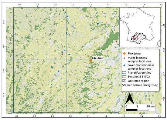
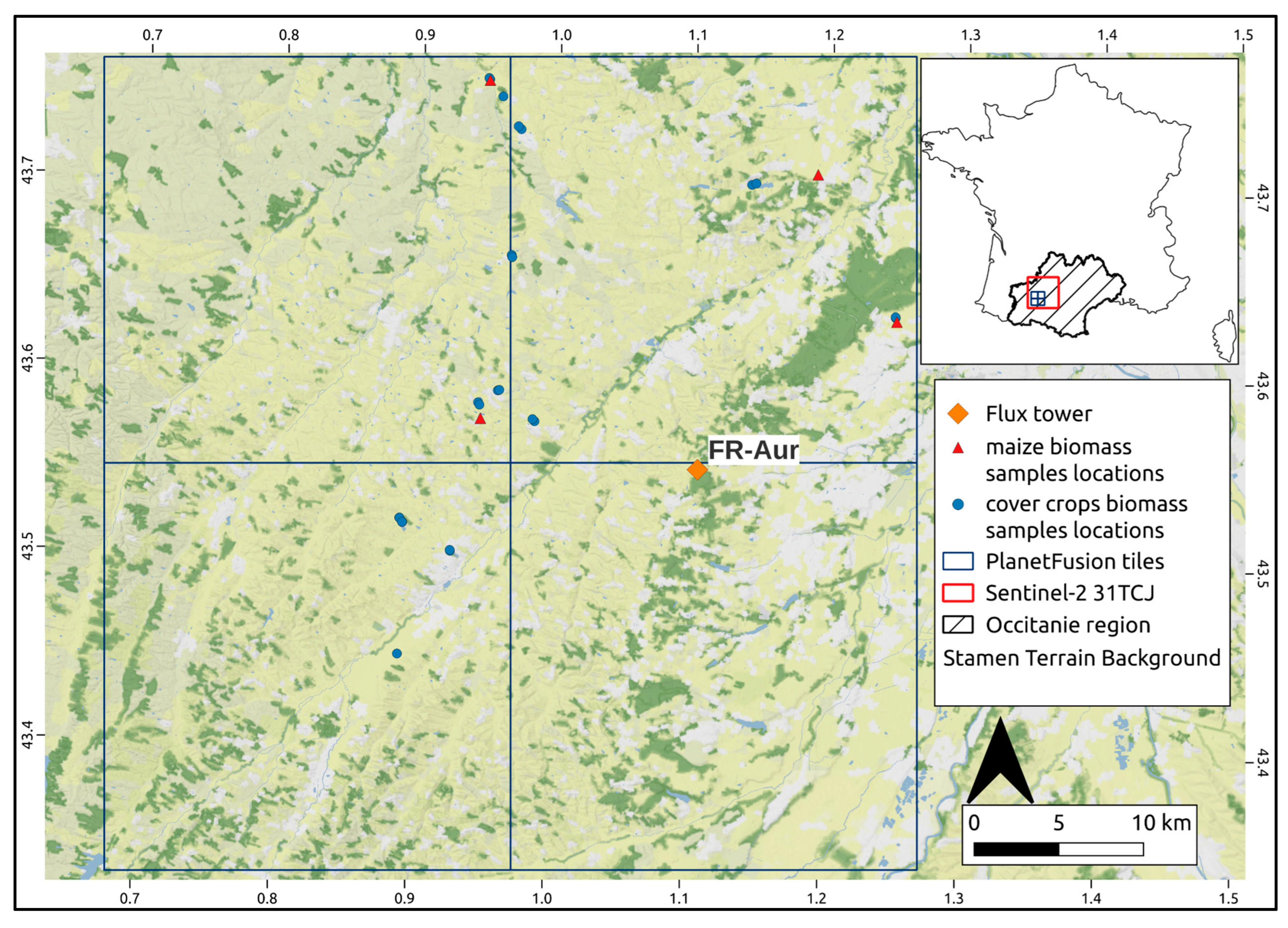
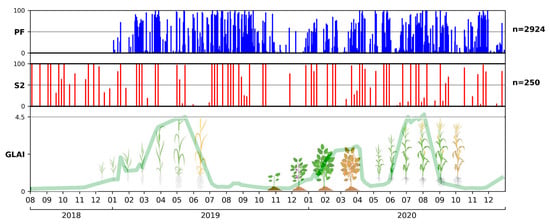
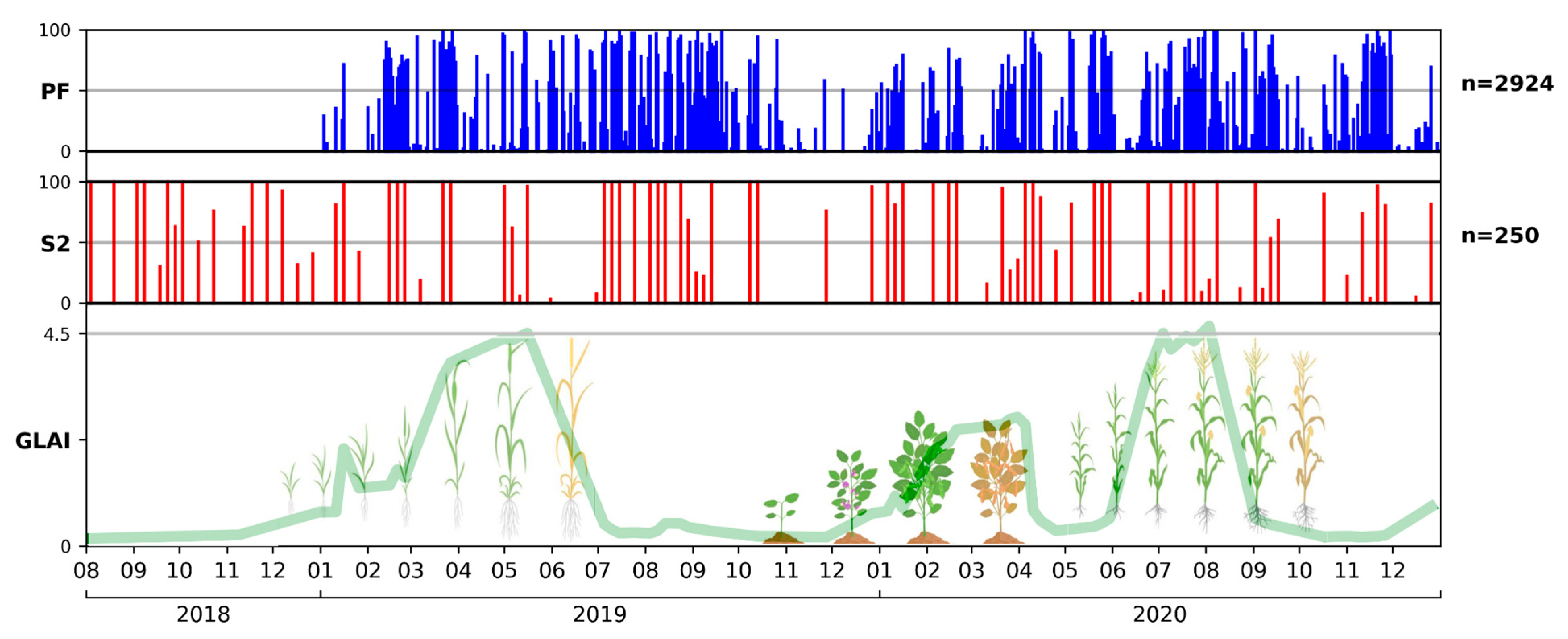
The area of interest is located in the Occitanie region (south-west France) and corresponds to 4 PF UTM tiles (13E-200N, 13E-201N, 14E-200N, and 14E-201N), which are located in the south-west part of the S2 tile 31TCJ (Figure 1). The study period, from 1 January 2019 to 31 December 2020, was selected based on the availability of PF data supplied to Netcarbon by Planet Labs (Planet Labs PBC, San Francisco, CA, USA). Cumulative annual precipitation and mean annual temperature are 758.4 mm and 13.6 °C in 2019, respectively [35], and 624.6 mm and 13.2 °C in 2020, respectively [36]. Cloud cover in this region is typically low in summer and variable between fall and spring, facilitating multitemporal optical remote sensing analysis of vegetation development (Figure 2). The study area is mainly occupied by crop fields (~90%), with winter wheat being the main crop, covering approximately 30% of the cultivated area. The agriculture in the Occitanie region represents 31% of the national soft wheat production, 36% of the national maize production, and 14% of the national fava bean production [37]. Consequently, we chose to analyze winter wheat, maize and fava bean cover crops. Winter wheat is typically sown in autumn (between mid-October and mid-November) and harvested in July of the next year. Maize is sown in April or May and harvested in September (silage maize) or October (grain maize) of the same year. Winter cover crops (e.g., fava bean, phacelia) are typically cultivated after a winter wheat crop and before a maize crop (sown in September or October and destroyed between December and April of the next year). Figure 2 shows the vegetation cycles of a typical winter wheat–cover crop–maize crop rotation.

Figure 1. Map of the area of interest. Stamen Terrain Background, the Planet Fusion tile limits, locations of the FR-Aur ICOS flux measurement site, of the maize AGB measurements (4 fields), and of the cover crops AGB measurements (19 fields). The map of France shows the location of the Planet Fusion tiles within the Sentinel-2 31TCJ tile limits, and the area of the Occitanie region.

Figure 2. Percentage of pixels kept after the pre-processing filter for each day over the 4 Planet Fusion tiles (top), percentage of cloud-free pixels in the Sentinel-2 31TCJ tile data located in the bounding box of the 4 Planet Fusion tiles (center), and schematic representation of a winter wheat–cover crop–maize agricultural cycle from the end of 2018 to the end of 2020 with the GLAI estimates computed from a field with this cropping cycle (bottom).

2.2. Remote Sensing Data

This study investigates the impact of assimilating optical remote sensing data (PF) with higher spatial and temporal resolutions into AgriCarbon-EO, compared to the reference S2 data, for estimating CO₂ flux components (NEE, GPP, Reco) and crop production (AGB, yield). A summary of the spectral band characteristics of S2 and PF data and availability of the remote sensing data used in this study is shown in Table 1 and Figure 2, respectively.

Table 1. Sentinel-2 and Planet Fusion spectral band characteristics.

	Sentinel-2	Planet Fusion
Band Name	Wavelength [µm] (Resolution [m])	Wavelength [µm] (Resolution [m])
Blue	447–545 (10)	450–510 (3)
Green	537–582 (10)	530–590 (3)
Red	645–683 (10)	640–670 (3)
Red-edge 1	694–713 (10, resampled)
Red-edge 2	731–749 (10, resampled)
Red-edge 3	768–796 (10, resampled)
NIR	762–907 (10)
NIR2	848–881 (10, resampled)	850–880 (3)
SWIR1	1542–1756 (10, resampled)
SWIR2	2081–2323 (10, resampled)
Availability	5 days	daily

2.2.1. Planet Fusion Data

Planet Labs provided Netcarbon with PF v.1.0.0 data for an area covering four PF tiles (731 images per tile, totaling 2924 images) in 2022. PF aims to deliver radiometrically and geometrically harmonized, sensor-agnostic surface reflectance data from the PlanetScope (PS) constellation. The PS constellation, comprising three CubeSat generations, has historically faced interoperability and cross-calibration challenges due to radiometric differences among its 150+ sensors [38]. PF adopts an implementation of the CESTEM algorithm to harmonize and inter-calibrate multi-constellation data streams from PS, S2, L8/L9, MODIS and VIIRS [34,39]. PF uses the Framework for Operational Radiometric Correction for Environmental Monitoring (FORCE) [40] to generate a harmonized Sentinel-2 and Landsat 8/9 BRDF adjusted SR product to be used as the calibration target during the CESTEM-based harmonization step. The resulting PF product (PF-SR) is delivered daily with a 3 m resolution and for 4 spectral bands (Table 1). A temporally driven functionality is used for cloud and cloud shadow identification and masked pixels are gap-filled using available multi-source imagery close to the date of interest with spatial and temporal interpolation techniques [34]. Each PF-SR product comes with a quality assurance (PF-QA) product that includes traceability information about the scene data used for PF-SR pixel creation and gap-filling, cloud mask labels, and pixel-level uncertainty estimates for each spectral band. The PF processing underwent significant refinements between the v1.0.0 used in this article, and the current v1.4.0. The pixel reflectance uncertainty is strongly related to the period of time between the latest clear-sky observation data and the PF date of interest [34]. To ensure PF data accurately represents crop cycle evolution, pixels are pre-processed by filtering out those with 100% gap-fill indicated by PF-QA, or where observation data used for gap-filling are more than 15 days from the PF image date of interest. Pixels for which the PF-QA indicated cloud and cloud shadow presence are also filtered out.

2.2.2. Sentinel-2 Data

S2 imagery is extensively used in agricultural remote sensing [41]. Given the demonstrated robustness of LAI retrieval from PROSAIL inversion using Sentinel-2 data [42], S2-derived estimates are considered our reference in this study. Top of Canopy L2A S2 reflectances are retrieved from the Thematic Center for Continental Surfaces (THEIA) platform, with the MAJA processing chain [43] for atmospheric correction and cloud masking applied. The spectral bands 5, 6, 7 and 8a are re-sampled from 20 m to 10 m resolution using the nearest neighbor method. The bands 1, 9 and 10, originally at 60 m resolution and designated for cloud screening and atmospheric correction, are excluded from this study. The resulting S2 data used in this study then have 10 spectral bands (Table 1) from 400 to 2500 nm at 10 m resolution.

2.3. Validation Datasets

Validation of AgriCarbon-EO’s estimates for CO₂ flux and crop production components (i.e., NEE, GPP, Reco, AGB and yield) relies on several datasets, as presented in Table 2. These datasets are extracted from the Environmental Information System (SIE) database maintained by the Centre d’Etudes Spatiales de la BIOsphère (CESBIO) [44].

Table 2. Summary of the CO₂ flux and dry aboveground biomass validation datasets.

Year	Crop	N° Fields	AGB Samples	Flux Measurements
2019	Wheat	1	0	1
2020	Maize	4	22	0
2020	Cover crops	19	29	0

2.3.1. CO₂ Fluxes

CO₂ fluxes data collected at our experimental site allow to quantify the CO₂ absorption by plants (photosynthesis, GPP) and CO₂ released by plants (autotrophic respiration, Ra) and soil organisms (heterotrophic respiration, Rh), as well as the net CO₂ flux (NEE) resulting from those processes. Combined with carbon exports (harvested biomass) and carbon imports as organic matter, CO₂ flux data enable the computation of the net annual crop carbon budget. The CO₂ flux data (GPP, Reco, which is the sum of Ra and Rh, as well as NEE) are retrieved from the Auradé (FR-Aur) cropland flux site belonging to the Integrated Carbon Observation System (ICOS). FR-Aur is located in the south-west of Toulouse (Figure 1). Net CO₂ fluxes are measured using the Eddy Covariance method [45], which employs a 3D sonic anemometer and an open-path infrared gas analyzer, as described by [10]. The NEE (gC.m⁻².d⁻¹) is then partitioned into GPP and Reco according to the method described in [10] and adapted from [46]. The conservative approach of [10], which positions the flux tower mast at the field center to optimize its footprint and filters data where more than 10% of the flux signal originates from outside the field, ensures that measured fluxes are representative of the field. Accordingly, AgriCarbon-EO flux estimates are averaged at the field scale before validation against in situ data. The quality of the observed flux components is assessed with the quality flags from the FLUXNET archive (https://fluxnet.org/). As the flux measurements are computed and recorded every 30 min, their values and associated quality flags are aggregated to a daily time step prior to the comparison with daily AgriCarbon-EO estimates. Daily values containing over 50% low-quality data are excluded from the statistical analysis. The CO₂ fluxes are analyzed over a winter wheat cropping year (1 October 2018 to 30 September 2019).

2.3.2. Dry Aboveground Biomass

The Elementary Sampling Unit (ESU) protocol [29] is employed to measure dry AGB in maize and fava bean fields. The ESU protocol consists of sampling the aboveground vegetation over one or two square meters (i.e., sub samples) at five locations in an area of 10 × 10 m. The sub samples are collected in a cross pattern within the 10 m × 10 m square. Each sample is weighted in the field (fresh biomass). Then, the sample collected at the center of the cross is oven dried to measure dry AGB in the lab. The mean and standard deviation of ESU dry AGB (g.m⁻²) are then calculated by applying the relative humidity measured for the central sample to the other four sub samples. The coordinates of the ESU are measured with a GPS at the location of the central sub sample. In 2020, the maize AGB was measured in four fields within the footprint of the PF tiles during two periods (July and September). Regarding cover crops, a field campaign was conducted in 2020 (over 19 fields between January and April).

Since in situ AGB values are estimated over a 10 m × 10 m square, AGB estimates and uncertainties from PF simulations are averaged over a 3 pixels × 3 pixels matrix, with the central pixel aligned with the ESU coordinates.

2.4. The Agricarbon-EO Processing Chain

AgriCarbon-EO v.1.0.1 [12] is a processing chain that estimates cropland carbon and water budget components, including AGB, yield, and the daily dynamics of CO₂ fluxes (NEE, GPP, Reco), evaporation, transpiration, and soil water content. A detailed description of the chain can be found in [12]. The processing is achieved in four steps.

The first step involves pre-processing initialization based on a land cover map, followed by automatic download and preparation of the processing database (weather, soil, satellite, and activity data).

The second step is the estimation of the GLAI dynamics and uncertainties from the satellite data by inversion of the PROSAIL radiative transfer model [33], through a spatial Bayesian approach (BASALT) combining normalized importance sampling and look-up tables (LUT). The priors used for this step (Table 3) are crop-specific for wheat and maize, and are sourced from [47]. Crop-specific parameters in PROSAIL inversion address equifinality by constraining the parameter space to realistic biophysical ranges (e.g., LAI, chlorophyll concentration, leaf angle) unique to each species. For cover crops, a non-specific parameterization [12] is used, as the studied area encompasses a mix of several species (i.e., fava bean, phacelia, and others). To ensure the retrieval of the GLAI, chlorophyll contents are limited to the highest concentrations. The soil brightness is influenced by the soil moisture index (psoil), as the soil brightness scaling term (rsoil) is set to 1 for each parametrization. The GLAI retrieval by PROSAIL inversion requires solar and satellite zenith and azimuth angles for each satellite image. The Planet Fusion SR data represent Normalized BRDF Adjusted Reflectances (NBAR) as the Landsat 8/9 and Sentinel-2 data used for cross-calibration have been normalized to nadir view [34]. As the PlanetScope sensors are near-nadir viewing natively (~4° field of view), the satellite view angle can be assumed to be zero. The PF data do not include corrections for sun angles and, as information on solar angles are not provided in the provided version of the PF metadata, the solar angles are computed.

Table 3. PROSAIL prior parameters configuration used in the Bayesian inversion. Wheat and maize priors from [47], cover crop priors from [12].

Name	Description	Unit	Wheat Priors (Uniform, [min max])	Maize Priors (Uniform, [min max])	Cover Crop Priors (Uniform, [min max])
N	Leaf structure parameter	-	[1, 3]	[1, 3]	[1, 2]
mean_LA	Mean Leaf Angle	°	[70, 80]	[70, 80]	[45, 65]
Cab	Chlorophyll a + b concentration	µg.m−2	[60, 80]	[60, 80]	[60, 80]
Car	Carotenoid concentration	µg.m−2	[5, 20]	[5, 20]	[5, 20]
cm	Leaf thickness	g.m−2	[0, 0.005]	[0, 0.005]	GLAI × 0.004 + [−0.02, 0.02]
GLAI	Green Leaf Area Index	m2.m−2	[0, 7]	[0, 7]	[0, 7]
psoil	Soil moisture index	-	[0, 1]	[0, 1]	[0, 1]
cw	Leaf water content	µg.m−2	[0.018, 0.02]	[0.016, 0.02]	0.01
hspot	Hotspot parameter	-	[0, 0.4]	[0, 0.4]	0.1

The image acquisition time is set to 10:20 AM UTC, to align as closely as possible with the S2 image acquisition time. Solar zenith and azimuth angles are computed using the formulas from [48,49] respectively. The PF-QA provides relative pixel uncertainty for each spectral band, linked to the observation images used for gap-filling, and a clear-sky uncertainty of 3% [34]. This relative uncertainty is included into the Bayesian framework to compute the PF GLAI uncertainties in the PROSAIL inversion. The PF-QA uncertainties were incorporated the same way Sentinel-2 reflectance uncertainties were incorporated in the PROSAIL inversion in [12], with the intent to allow a likelihood computation taking account of the reflectance uncertainties. As such, the equation of the log-likelihood is as follows [12] (Equation (1)):

$$log{L}_{i,j} =\sum (-0.5log(2\pi {({\sigma }_{i,j})}^2)) -(v_{i,j} - {\mu }_{i,j}^2)/(2{\sigma }_{i,j})$$

(1)

where $v$ is the simulated reflectances with PROSAIL value, $\mu$ and $\sigma$ are the mean and standard deviation of the observed reflectances by the satellites at top of canopy (after atmospheric corrections), respectively, j is the index for each simulated band, and i is the index for the model run.

The third step involves assimilating the estimated GLAI time series into the SAFYE-CO2 agronomic model [29,30] to estimate crop production and carbon budget components (NEE, GPP, Reco, AGB, yield) dynamics, also using the BASALT method. Prior parameters used for the different crop species in this study are taken from [12]. The weather data (daily average air temperature, cumulative global incoming solar radiation, daily potential evapotranspiration, and cumulative rainfall) used in this step are collected from the ERA5-Land database [50] through the dedicated API. ERA5-Land provides semi-hourly information on a ~9 km spatial grid.

The last step is the creation of maps of the biophysical variables of interest and their associated uncertainties over the area of interest.

2.5. Statistical Matching of Planet Fusion and Sentinel-2 Based GLAI

Spectral information in the red-edge region (700 to 800 nm) is known to enhance the accuracy of vegetation biophysical variable retrieval [42,51,52,53]. This is attributed to chlorophyll and leaf scattering, which more strongly reflect light in this spectral region [54]. LAI estimations lacking red-edge spectral information tend to overestimate low LAI values compared to field observations [55]. Since PF data lack red-edge spectral information, a statistical correction using cumulative density function (CDF) matching is applied to PF-based GLAI data to mitigate potential overestimation of low GLAI. CDF matching, also known as histogram matching, consists of matching the pixel value distribution of an input image (PF) to the pixel distribution of a target image (S2). Input and target GLAI CDFs are computed, and then the input GLAI value at a given threshold is mapped to the target GLAI value with the same probability.

Correcting all PF GLAI estimations requires a S2 CDF for each day of the simulation, which implies a S2-derived GLAI distribution every day. To compute a pseudo S2-based GLAI distribution for a date between two S2 image dates, the daily differences between the date of interest (DOI) and the two closest S2 dates (DOI_S2_prior and DOI_S2_posterior) are first calculated (Equations (2) and (3)):

$$D1 =DOI -DOI\_S2\_prior$$

(2)

$$D2=DOI\_S2\_posterior-DOI$$

(3)

The GLAI distribution for the date of interest (GLAI_i) is then computed as the weighted mean of the GLAI distributions from the closest prior and posterior S2 dates (GLAI_S2_prior and GLAI_S2_posterior, respectively). The inverse of the daily distances serves as weight, ensuring that GLAI estimates from the closest date received the highest weighting (Equation (4)):

$$GLA{I}_i = {\displaystyle \frac{GLAI\_S2\_prior/D1 + GLAI\_S2\_posterior/D2}{1/D1 + 1/D2}}$$

(4)

This results in an S2-based GLAI distribution for each day of the simulation. The CDFs of these GLAI distributions (hereafter referred to as correction CDFs) are computed from the probability density function (PDF) of the S2-derived GLAI distribution, which in our case is a histogram of GLAI values with 700 bins (ranging from 0.00 to 6.99, with a 0.01 step). The CDF is then calculated as the cumulative sum of the percentages of the PDF values at each bin (Equation (5)):

$$CDF= \sum _{n=0}^{n=6.99}{\displaystyle \frac{PDF}{nGLAI}}$$

(5)

This process results in a correction CDF for each day of the simulation. These correction CDFs are then integrated into the AgriCarbon-EO processing chain to correct PF GLAI estimations following the PROSAIL inversion step.

CDF values of the PF-based GLAI data are computed following Equation (5) and matched to the corresponding correction CDF for each day of simulation. Given a GLAI value X, the input probability P_i(X) is related to the target probability P_t(X′). The matching procedure can thus be written as (Equation (6)):

$$X’ = {Pt}^{-1}Pi\left(X\right)$$

(6)

This results in a corrected PF-based GLAI matched to S2-derived GLAI for the same date. CDF matching is applied at the field scale (i.e., each simulated field in the ACEO simulation has its own CDF).

2.6. Analysis of Planet Fusion’s Impact on AgriCarbon-EO’s Simulations

This study aims to compare CO₂ flux components and crop production estimations derived from AgriCarbon-EO using PF data only, against estimations based on S2 data only, and derived from the combined use of PF and S2 data. Several aspects are evaluated, including differences in radiometric/spectral resolution (10 spectral bands for S2 data vs. 4 for PF data) and image availability (every five days for S2 data vs. daily for PF data). Simulations based on S2 and PF data are hereafter referred to as S2-10bds and PF_daily, respectively, while simulations using the corrected PF GLAI estimates are referred to as PF_corr_daily. We evaluated the solutions using standard evaluation metrics: R², RMSE, and bias.

To analyze the impact of the number of spectral bands in the PROSAIL inversion, GLAI estimates from S2-10bds, S2 limited to the native 10 m spectral bands (S2-4bds), PF_daily, and PF_corr_daily are retrieved from 50 randomly distributed 30 m × 30 m squares for each crop type and compared. GLAI means and standard deviations (std) are compared for each crop according to crop phase (emergence, maximum growth, and senescence). Winter wheat emergence is set between 1 January 2019 and 28 February 2019 (to avoid the effect of the lack of PF data in 2018), maximum growth between 1 March 2019 and 30 April 2019, and senescence between 1 May 2019 and 30 June 2019. As cover crops are destroyed before they reach senescence, their periods of development are set between 1 November 2019 and 31 December 2019 (emergence), 1 January 2020 and 29 February 2020 (growth), and 1 March and 30 April (maximum growth). Maize phases are set between 1 May 2020 and 30 June 2020 (emergence), 1 July 2020 and 31 August 2020 (maximum growth), and 1 September and 31 October (senescence).

We then compare the NEE, GPP, Reco and AGB estimates from S2-10bds, PF_daily, and PF_corr_daily to estimate the impact of the spectral difference and temporal availability.

The combined use of S2 and PF data in comparison with the use of S2 or PF data alone is evaluated by comparing CO₂ flux and AGB estimates from two additional simulations (S2_PF, and S2_PF_corr) with S2-10bds, PF_daily and PF_corr_daily estimates. PF data are averaged to a 10 m grid in those simulations.

Comparisons of Net Ecosystem Productivity (NEP, the cumulated NEE over a cropping year), and yield estimations (AGB × harvest index) are also made at the scale of one PF tile for winter wheat in 2019, and maize in 2020. The Registre Parcellaire Graphique (RPG) issued by the Institut National Geographique (IGN) is used to retrieve the cropland maps in the PF tile areas. The harvest index was set to 0.45 for winter wheat, and 0.49 for maize. Each distribution normality is tested with the Shapiro–Wilk test, and the Levene test is conducted to estimate variance homogeneity. For each variable, global difference significance between all distributions is tested with a one-way ANOVA if all distributions are found to be normal and all variance homogenous. The Welch test is used if the variances are heterogeneous. If the distributions are found not normal, the Kruskal–Wallis test is conducted. Post hoc comparisons are conducted if the preceding tests yield significant results.

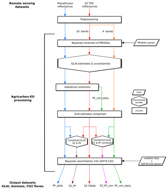
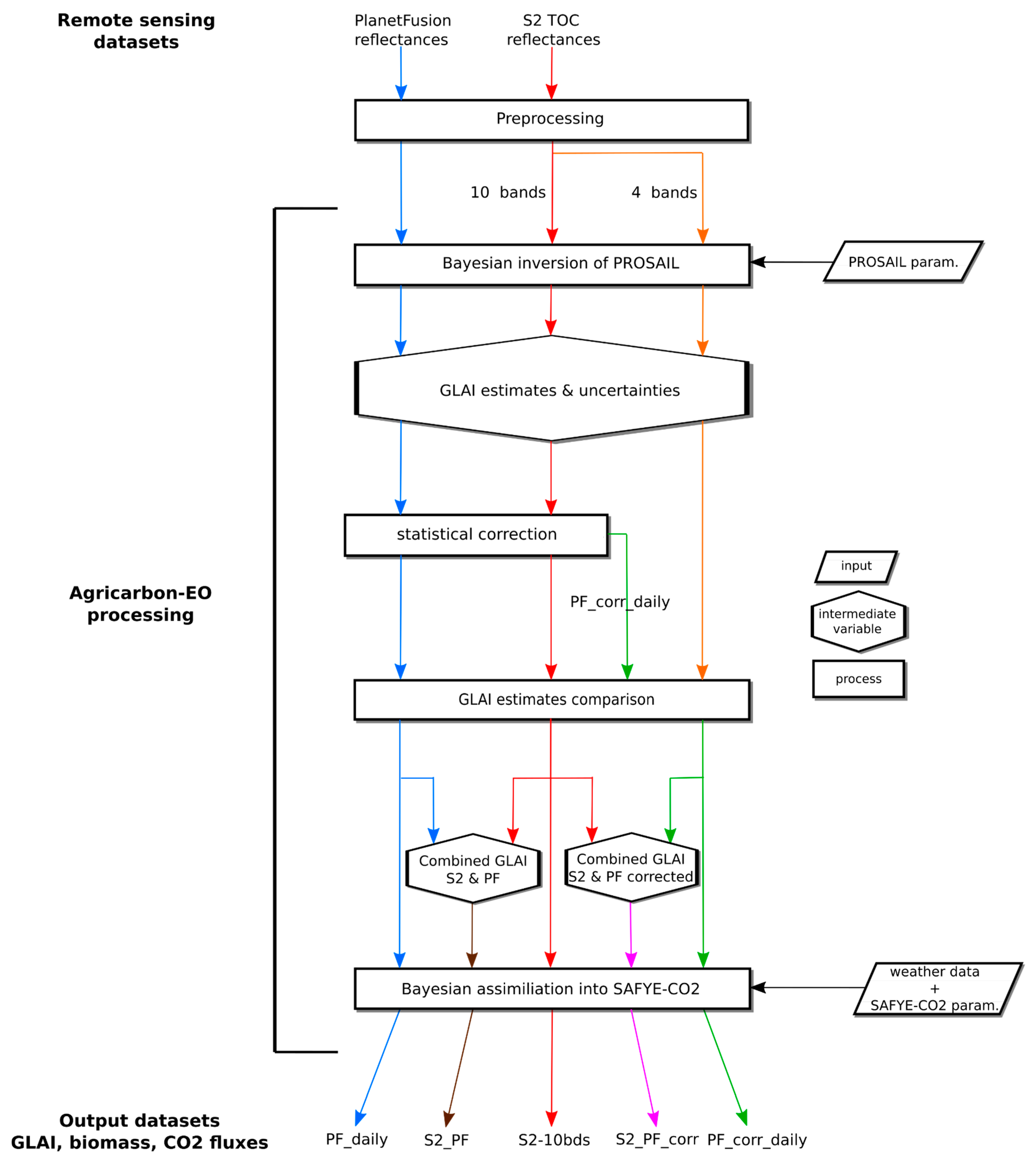
A summary of the workflow with the aim of each image type simulation is shown in Figure 3.

Figure 3. Diagram showing the workflow and comparative datasets obtained using Planet Fusion, Sentinel-2 with 4 and 10 bands spectral bands, along with the combined use of Sentinel-2 and Planet Fusion.

3. Results

3.1. Comparison of GLAI Estimates

Table 4 presents GLAI derived from S2-10bds, S2-4bds, PF_daily, and PF_corr_daily simulations. GLAI values obtained with four band simulations (PF_daily and S2-4bds) are highest across all crop phases. The largest mean differences are observed during the winter wheat and cover crop emergence periods between S2-10bds and PF_daily (0.8 m².m⁻² and 0.9 m².m⁻², respectively). Most of the highest mean GLAI estimates are obtained using PF_daily. The statistically corrected estimates closely align with S2-10bds GLAI, with exceptions during winter wheat senescence (3.82 m².m⁻² with S2-10bds, and 2.31 m².m⁻² with PF_corr_daily), and maize maximum growth (3.19 m².m⁻² with S2-10bds, and 2.41 m².m⁻² with PF_corr_daily). The scarcity of usable S2 data in June 2019 and August 2020 strongly impacts the statistical correction’s performance during those periods.

Table 4. Mean and Std of GLAI distributions from the PROSAIL inversion over the emergence, maximum growth and senescence crop phases in winter wheat fields in 2019 (50 samples), cover crop fields in 2019 and 2020 (50 samples for each year), and maize fields in 2020 (50 samples). The highest GLAI mean estimates for each crop period are indicated in bold.

Crop	Period	S2-10bds Mean ± Std	S2-4bds Mean ± Std	PF_Daily Mean ± Std	PF_Corr_Daily Mean ± Std
winter wheat	emergence	1.21 ± 1.12	1.61 ± 1.29	2.11 ± 1.01	1.22 ± 0.78
	max growth	2.59 ± 0.92	2.81 ± 0.85	2.85 ± 0.76	2.74 ± 0.99
	senescence	3.82 ± 0.69	3.91 ± 0.53	3.15 ± 0.85	2.31 ± 1.46
cover crop	emergence	1.19 ± 1.60	0.91 ± 0.82	1.99 ± 1.58	1.84 ± 1.50
	growth	2.36 ± 1.91	1.78 ± 1.20	2.99 ± 1.17	2.88 ± 1.16
	max growth	1.38 ± 1.95	1.13 ± 1.34	1.63 ± 1.37	1.62 ± 1.37
maize	emergence	1.06 ± 1.01	1.23 ± 1.11	1.27 ± 0.98	1.08 ± 0.89
	max growth	3.19 ± 0.77	3.36 ± 0.73	2.81 ± 0.52	2.41 ± 0.99
	senescence	1.39 ± 1.11	2.02 ± 1.42	1.71 ± 1.02	0.93 ± 0.83

3.2. Evaluation of CO₂ Fluxes

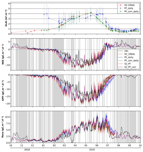
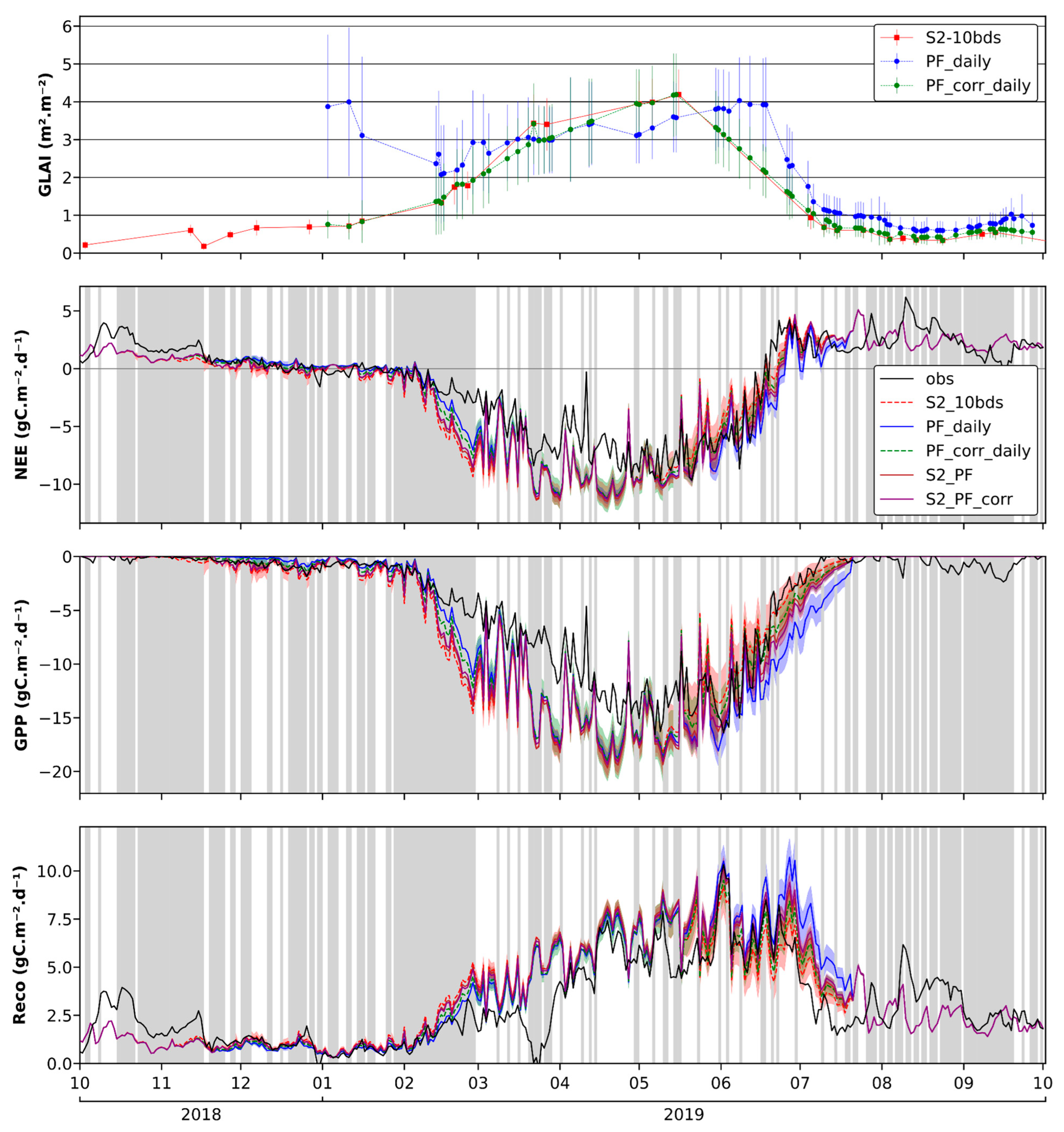
Figure 4 illustrates GLAI dynamics from the PROSAIL inversion for S2-10bds, PF_daily, and PF_corr_daily, alongside spatially averaged daily CO₂ flux (NEE, GPP, Reco) outputs from S2-10bds, PF_daily, PF_corr_daily, and S2_PF simulations. Simulated CO₂ flux components are compared against the flux derived from in situ measurements at the FR-Aur site. Corresponding statistics for the winter wheat cycle (30 November 2018 to 5 July 2019) are presented in Table 5.

Figure 4. GLAI dynamics from the PROSAIL inversion obtained with S2-10bds, PF_daily, PF_corr_daily, S2_PF and S2_PF_corr (top), and time series of winter wheat NEE, GPP and Reco (bottom) at the FR-Aur site in 2018–2019, and from AgriCarbon-EO S2-10bds, PF_daily, PF_corr_daily, S2_PF, and S2_PF_corr. Regarding the CO₂ flux components, the colored line surface represents the mean and standard deviation of the posterior distribution, and the black solid line the CO₂ fluxes observations at FR-Aur. Gray vertical bars indicate the days during which more than 50% of the observation data are gap-filled.

Table 5. Statistics for the NEE, GPP and Reco in FR-Aur over the wheat cycle (30 November 2018 to 5 July 2019). The highest R² and the lowest RMSE and bias scores for each flux measurement are indicated in bold.

	Statistic	S2-10bds	PF_Daily	PF_Corr_Daily	S2_PF	S2_PF_Corr
NEE (gC.m−2.d−1)	R2	0.72	0.76	0.76	0.75	0.77
	RMSE	2.52	2.49	2.34	2.57	2.49
	Bias	0.94	1.34	0.99	1.33	1.31
GPP (gC.m−2.d−1)	R2	0.75	0.82	0.82	0.82	0.83
	RMSE	3.40	3.52	3.08	3.54	3.45
	Bias	1.61	2.35	1.65	2.30	2.31
Reco (gC.m−2.d−1)	R2	0.80	0.84	0.85	0.85	0.86
	RMSE	1.29	1.54	1.19	1.40	1.42
	Bias	−0.66	−1.01	0.66	−0.97	−0.99

Overall, simulated NEE, GPP and Reco dynamics accurately reproduce flux tower observations during emergence, parts of the growing season (March 2019), and senescence. However, NEE and GPP are underestimated in April and May, prior to maximum crop development, compared to measurements, probably partly because the emergence date was set late (in January) to overcome the lack of PF data in 2018. Despite this lack of PF data in 2018 (Figure 2), PF_daily and PF_corr_daily CO₂ fluxes and GPP simulations are, overall, very similar to the other simulations.

Periods with the poorest fit correspond to dates flagged as low quality (i.e., over 50% of data are gap-filled on those dates) and are excluded from statistical computations. GPP and Reco observation data from mid-March to April 2019, resulting from a previously reported parsing error [12], are excluded from statistical computation.

Flux dynamics from PF simulations appear to fit better than S2 simulations during the early growth phase (February–March 2019), despite abnormally high GLAI values (>2 m².m⁻²) and associated uncertainties in PF_daily estimates during this period. However, due to gap-filled observation data during this period, the superior performance of the PF_daily simulation cannot be definitively confirmed. The dynamic difference between S2-10bds and PF_daily stems from variations in GLAI estimation during the PROSAIL inversion in AgriCarbon-EO. Simulated GLAI dynamics show a strong overestimation with PF_daily estimates compared to S2 ones, except in May and June 2019. The statistical correction generally improves GLAI dynamics but slightly underestimates PF GLAI estimates compared to S2 GLAI between March and May 2019. The limited availability of S2 data during this period may prevent the correction CDF from accurately representing the field’s growth rate and heterogeneity. During senescence, the statistical correction aligns with the S2 GLAI dynamic but shows a gradually decreasing GLAI in June 2019, also attributable to the lack of S2 data during this period.

For the late senescence (June 2019) and post-harvest (July-August 2019) phases, S2-10bds-based net CO₂ flux estimates show a better fit with observed flux than PF_daily estimates (likely due to overestimated GLAI, ~1 m².m⁻²). Net CO₂ flux estimates from PF_corr_daily, S2_PF, and S2_PF_corr simulations fall between S2-10bds and PF_daily simulations throughout the crop cycle. During the growth phase, net CO₂ flux simulations based on PF_corr_daily dynamics are closer to PF_daily dynamics, while S2_PF dynamics are closer to S2-10bds. During senescence, both PF_corr_daily and S2_PF are closer to S2-10bds dynamics than to PF_daily dynamics.

The statistics in Table 5 show similar scores for NEE, GPP, and Reco between S2-10bds and PF_corr_daily. PF_daily, S2_PF, and S2_PF_corr exhibit similar R² values but higher RMSE and bias scores for NEE, GPP, and Reco compared to S2-10bds and PF_corr_daily. The elevated RMSE and bias scores for PF_daily, S2_PF, and S2_PF_corr are attributed to flux estimations during senescence, particularly in late May, June, and early July 2019, which deviate more significantly from observed values than S2-10bds and PF_corr_daily estimates during the same period. For S2_PF and S2_PF_corr, SAFYE-CO2 flux estimates during this period are exclusively driven by GLAI from PF data due to significant cloud cover precluding S2 data availability over the FR-Aur field, thus explaining the similar statistical scores with PF_daily. PF_corr_daily exhibits the best R² and RMSE scores for all fluxes, and the best bias score for Reco, during the winter wheat cycle.

Figure 4 and Table 5 indicate that using PF imagery, with or without correction, does not significantly improve the accuracy of CO₂ flux component estimates compared to S2 imagery.

3.3. Validation of Dry Aboveground Biomass Estimates

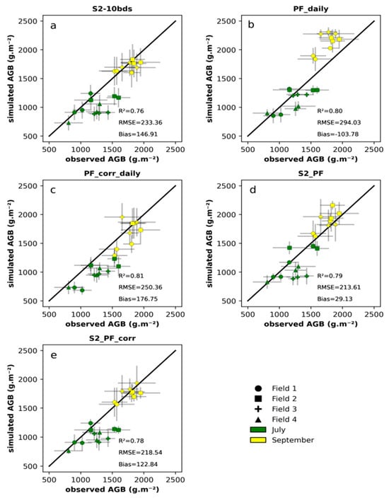
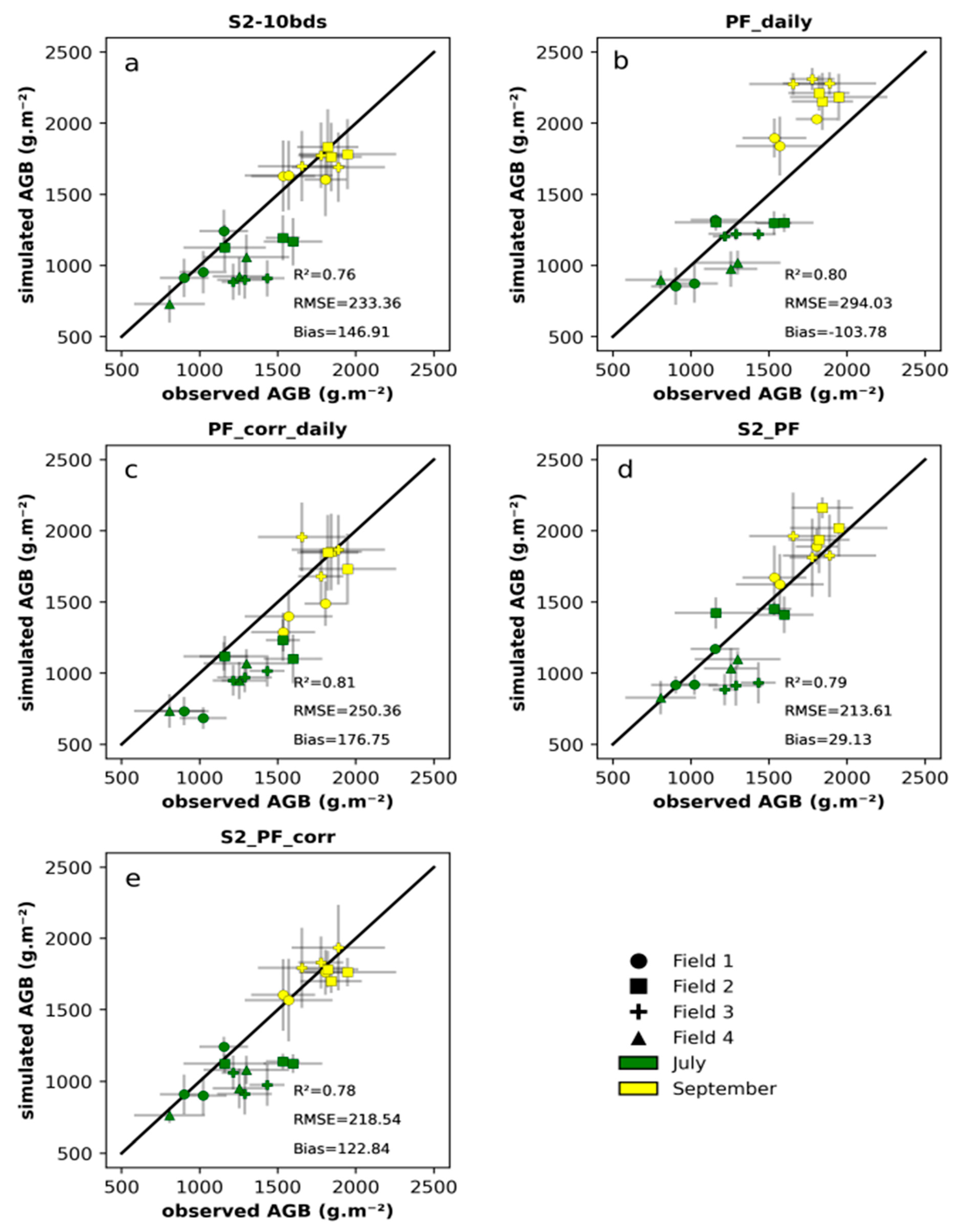
Figure 5 presents scatterplots of observed maize AGB versus simulated AGB for four fields in 2020. AGB observations were conducted during two field campaigns (July 2020, and September 2020, shortly before harvest). Associated statistics are shown in each scatter plot corresponding to the different modeling exercises (e.g., assimilating PF only).

Figure 5. Scatter plots of the simulated maize dry aboveground biomass (AGB) obtained from simulations using S2-10bds (a), PF_daily (b), PF_corr_daily (c), S2_PF (d) and S2_PF_corr (e) versus in situ dry aboveground biomass measured in four fields in 2020.

Overall, statistics demonstrate a good fit, with R² ranging from 0.76 (S2-10bds, Figure 5a) to 0.81 (PF_corr_daily, Figure 5c). PF_daily (Figure 5b) and PF_corr_daily (Figure 5c) simulations yield the most correlated results, with R² values of 0.80 and 0.81, respectively. However, their RMSE (294.03 and 250.36 g.m⁻², respectively) and bias (−103.78 and 176.75 g.m⁻², respectively) scores are higher than those of S2-10bds (RMSE = 233.36 g.m⁻², bias = 146.91 g.m⁻²). For PF_daily estimates, this is attributed to AGB overestimation in September, stemming from a higher GLAI estimation (~1 m².m⁻²) compared to S2-10bds estimates (~0.5 m².m⁻²). While this overestimation is corrected in the PF_corr_daily estimates, the statistical correction underestimates AGB values in July for field n°1, leading to slightly higher RMSE and bias scores than S2-10bds. This underestimation results from decreasing GLAI estimates in early August 2020 in the PF_corr_daily simulation, causing an earlier simulated senescence compared to the S2-10bds simulation, which occurred around mid-August 2020 for this field. This premature senescence is caused by the lack of available S2 data between the beginning of August 2020 (when GLAI ~3 m².m⁻²) and September 2020 (when GLAI ~0.7 m².m⁻²). The statistical correction gradually decreases GLAI estimates between these dates, which may not accurately reflect actual conditions.

The S2_PF and S2_PF_corr simulations (Figure 5d,e) demonstrate very good statistics, with R² scores (0.79 and 0.78, respectively) close to PF_daily (0.80) and PF_corr_daily (0.81). They also exhibit the lowest RMSE (213.61 and 218.54 g.m⁻², respectively) among all simulations, and S2_PF shows the lowest bias score (29.13 g.m⁻²).

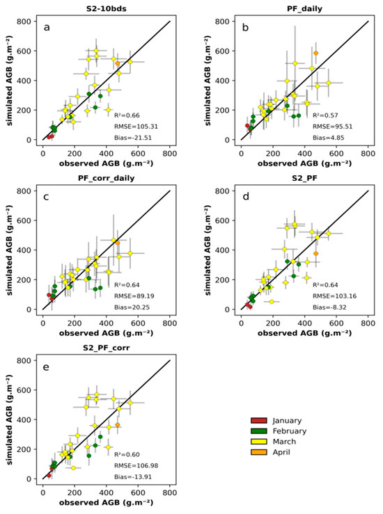
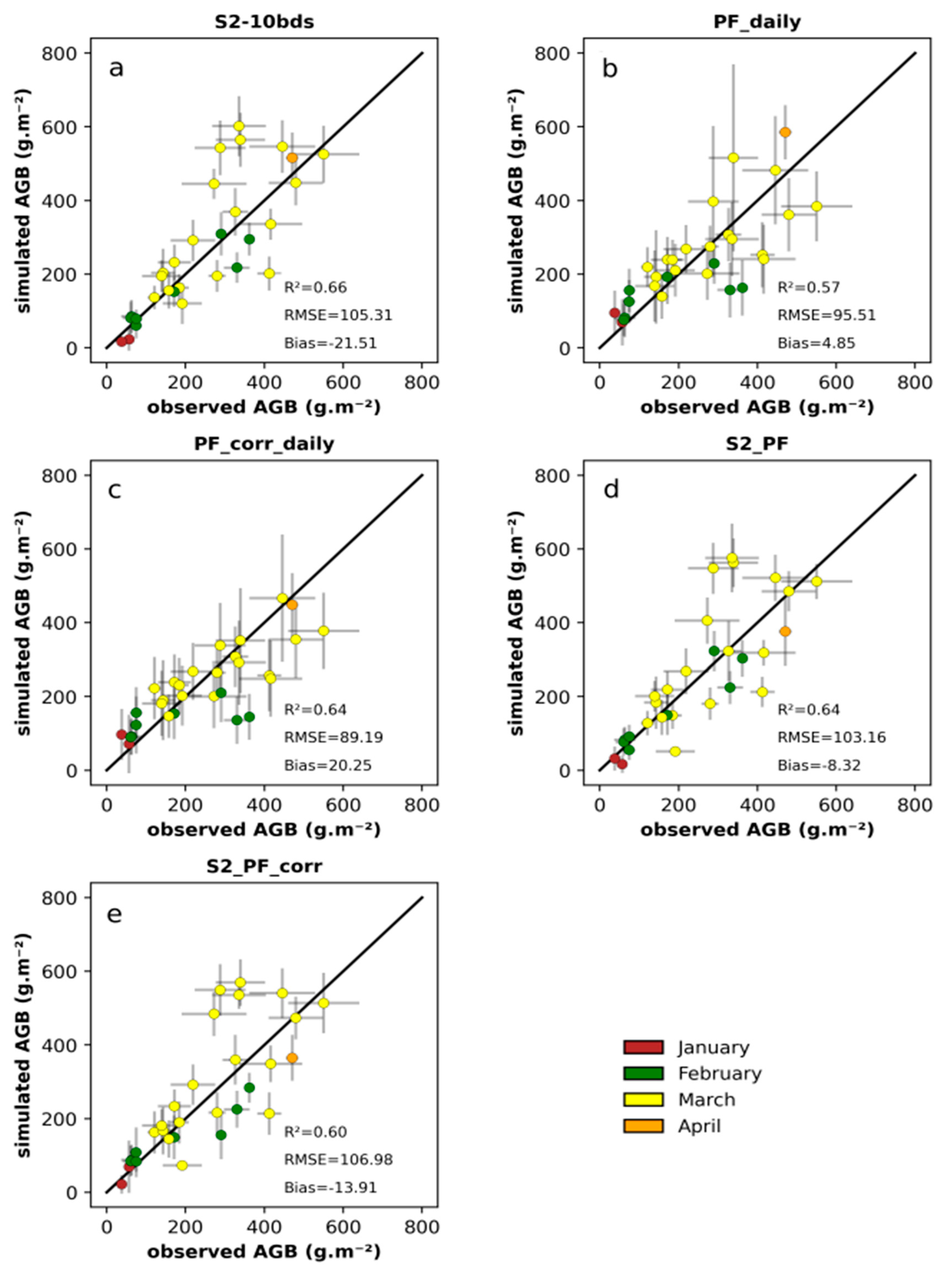
Figure 6 presents scatterplots of observed cover crop AGB versus simulated AGB in 2020. AGB observations were collected during several field campaigns (January, February, March, and April, shortly before destruction). Associated statistics are shown in each scatter plot. Overall, the statistics indicate a good fit, with R² ranging from 0.57 (PF_daily, Figure 6b) to 0.66 (S2-10bds, Figure 6a).

Figure 6. Scatter plots of the simulated cover crop dry aboveground biomass (AGB) obtained from simulations using S2-10bds data (a), PF_daily (b), PF_corr_daily (c), S2_PF (d), and S2_PF_corr (e) versus in situ dry aboveground biomass measured in 19 fields in 2020.

S2-10bds (Figure 6a) yields the most correlated results, with R² at 0.66. However, it also exhibits the second highest RMSE (105.31 g.m⁻²) and the highest negative bias (−21.51 g.m⁻²), attributed to the overestimation of some simulated AGB in March 2020 due to a lack of usable S2 data during that month. Consequently, SAFYE-CO2 simulates continuous vegetation growth during this period, which may not reflect actual conditions. PF_daily (Figure 6b) shows the lowest R² (0.57), the second lowest RMSE (95.51 g.m⁻²) and the lowest bias (4.85 g.m⁻²). Simulated AGB exhibits higher uncertainties than other simulations, stemming from the greater uncertainties in GLAI estimates from the PROSAIL inversion, which could not constrain the SAFYE-CO2 simulation with low uncertainties as effectively as S2-10bds. The statistical correction yielded similar statistical results to S2-10bds (R² = 0.64, RMSE = 89.19 g.m⁻², bias = 20.25 g.m⁻²), along with lower simulated AGB uncertainties.

Overestimation of some simulated AGB values in March 2020 is also obvious in S2_PF (Figure 6d) and S2_PF_corr (Figure 6e). This similarity is attributed to the higher PF GLAI uncertainties from the PROSAIL inversion, which prevented the SAFYE-CO2 simulation from deviating from the S2-10bds forcing. However, while these simulations exhibit similar R² (0.64 and 0.60, respectively) and RMSE (103.16 g.m⁻² and 106.98 g.m⁻², respectively) to S2-10bds, they also demonstrate lower bias (−8.32 g.m⁻² and −13.91 g.m⁻², respectively).

Figure 5 and Figure 6 indicate that ACEO simulations using PF data alone (native or corrected) do not yield improved AGB estimation accuracy compared to simulations with S2. However, incorporating S2 with PF imagery in a simulation reduces RMSE and bias compared to simulations with S2 alone.

3.4. Intercomparison of NEP and Yield Estimates

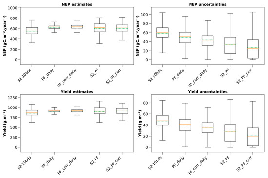
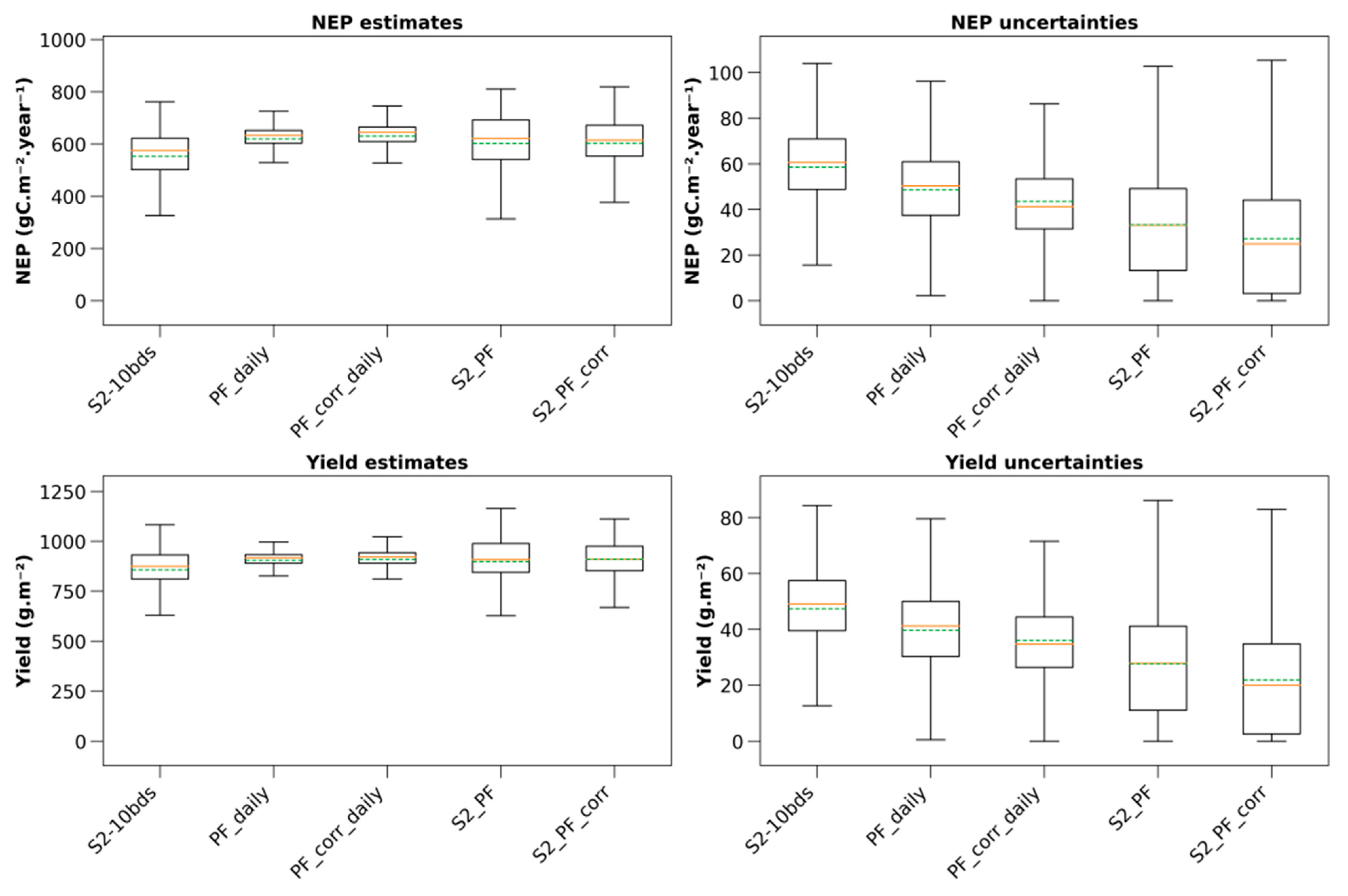
Figure 7 presents the estimates and associated uncertainties of NEP, yield and AGB for winter wheat in 2019 at the scale of the area covered by one of the PF tiles used in this study (Figure 1), covering 1813 fields. The NEP is computed from 1 October 2018 to 30 September 2019.

Figure 7. NEP estimates and associated uncertainties (top row), and yield estimates and associated uncertainties (bottom row) for 1813 winter wheat fields located in the area extent of one of the four PF tiles in 2019. Orange lines in the boxplots represent the medians and dashed green lines the means.

NEP estimates means are similar between all simulations (between 553.08 gC.m⁻².year⁻¹ (S2-10bds) and 630.19 gC.m⁻².year⁻¹ (PF_corr_daily)), which is also the case regarding the medians (between 575.43 gC.m⁻².year⁻¹ (S2-10bds) and 645.53 gC.m⁻².year⁻¹ (PF_corr_daily)). NEP estimates variabilities are also similar between all simulations (between 300 and 820 gC.m⁻².year⁻¹), with PF_daily and PF_corr_daily showing the smallest variabilities (between 500 and 750 gC.m⁻².year⁻¹ for both simulations). A similar observation can be made regarding the yield, as the estimates means (between 856.83 g.m⁻² (S2-10bds) and 910.62 g.m⁻² (S2_PF_corr)) and medians (between 874.79 g.m⁻² (S2-10bds) and 921.59 g.m⁻² (PF_corr_daily)) are also similar. Yield estimate variabilities are also similar (between 625 and 1170 g.m⁻²), with PF_daily and PF_corr_daily exhibiting the smallest variabilities (between 800 and 1050 g.m⁻² for both simulations). These smaller variabilities stem from the unavailability of PF data in late 2018 (Figure 2), although this did not significantly impact mean and median estimates compared to other simulations.

All NEP and yield estimate distributions show a non-normal distribution (Shapiro p-values << 0.05 for all distributions). Pairwise comparisons reveal that all NEP distributions are significantly different (Bonferroni p-values << 0.05), except for PF_daily and S2_PF, and for S2_PF and S2_PF_corr (Bonferroni p-values = 1 for both). For yield, pairwise comparisons indicate that all yield distributions are significantly different (Bonferroni p-values << 0.05).

Uncertainties for both variables show similar tendencies (NEP uncertainties: means between 27.21 gC.m⁻².year⁻¹ (S2_PF_corr) and 58.52 gC.m⁻².year⁻¹ (S2-10bds); medians between 24.95 gC.m⁻².year⁻¹ (S2_PF_corr) and 60.62 gC.m⁻².year⁻¹ (S2-10bds). Yield uncertainties: means between 21.86 g.m⁻² (S2_PF_corr) and 47.35 g.m⁻² (S2-10bds); medians between 19.92 g.m⁻² (S2_PF_corr) and 49.05 g.m⁻² (S2-10bds)). Uncertainty variabilities are generally consistent across all simulations for each variable (0–110 gC.m⁻².year⁻¹ for NEP, and 0–90 g.m⁻² for yield).

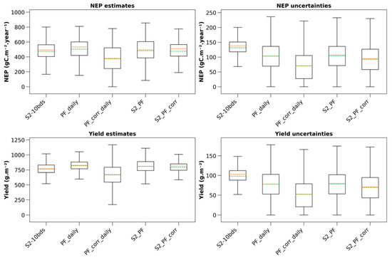
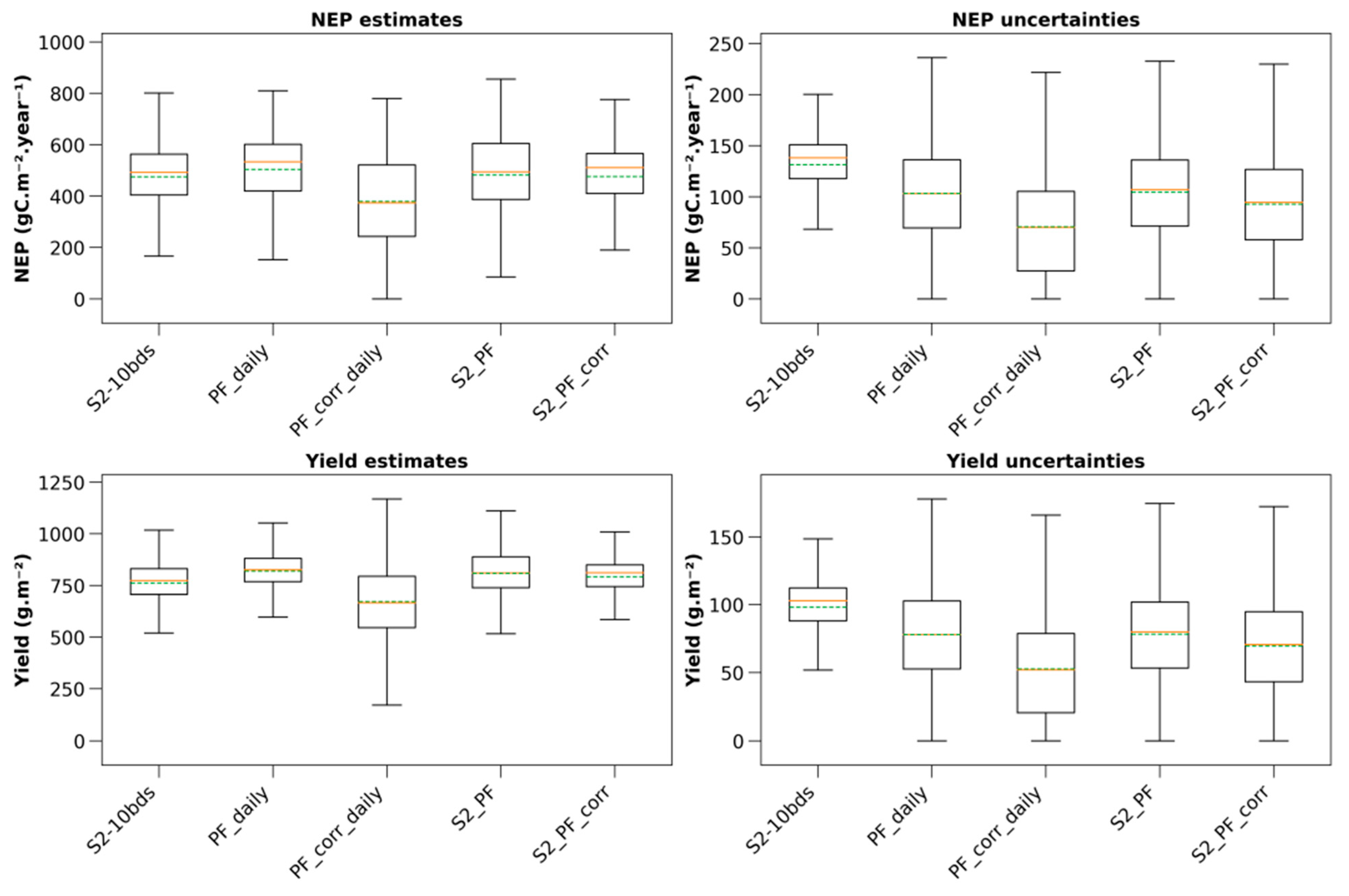
Figure 8 presents the regional estimates and standard deviations of NEP and yield for maize in 2020 at the scale of the area covered by one of the PF tiles used in this study (Figure 1), covering 384 fields. The NEP is computed from 1 January 2020 to 31 December 2020.

Figure 8. NEP estimates and associated uncertainties (top row), and yield estimates and associated uncertainties (bottom row) for 384 maize fields located in the area extent of one of the four PF tiles in 2020. Orange lines in the boxplots represent the medians and dashed green lines the means.

Similar to the winter wheat results (Figure 7), mean NEP estimates are comparable across all simulations (ranging from 379.46 gC.m⁻².year⁻¹ for PF_corr_daily to 504.06 gC.m⁻².year⁻¹ for PF_daily), as are the medians (from 373.98 gC.m⁻².year⁻¹ for PF_corr_daily to 533.49 gC.m⁻².year⁻¹ for PF_daily). NEP estimate variabilities are also similar across all simulations (between 80 and 860 gC.m⁻².year⁻¹), except for PF_corr_daily, which shows minimal values at 0 gC.m⁻².year⁻¹. A similar observation applies to yield estimate means (between 672.04 g.m⁻² for PF_corr_daily and 818.91 g.m⁻² for PF_daily) and medians (between 666.45 g.m⁻² for PF_corr_daily and 825.75 g.m⁻² for PF_daily). Yield estimates variabilities are also similar (between 500 and 1170 g.m⁻²), except for PF_corr_daily, which shows minimal values at 171 g.m⁻².

All NEP and yield estimate distributions exhibit non-normal distribution (Shapiro p-values << 0.05 for all distributions). Pairwise comparisons indicate that all NEP distributions are significantly different (Bonferroni p-values << 0.05), except for PF_daily and PF_corr_daily (Bonferroni p-value = 0.37). For yield, pairwise comparisons reveal that all yield distributions are significantly different (Bonferroni p-values << 0.05).

Uncertainties for both variables show similar tendencies (NEP uncertainties: means between 70.60 gC.m⁻².year⁻¹ (PF_corr_daily) and 131.40 gC.m⁻².year⁻¹ (S2-10bds); medians between 70.06 gC.m⁻².year⁻¹ (PF_corr_daily) and 138.12 gC.m⁻².year⁻¹ (S2-10bds). Yield uncertainties: means between 52.70 g.m⁻² (PF_corr_daily) and 98.16 g.m⁻² (S2-10bds); medians between 51.94 g.m⁻² (PF_corr_daily) and 102.93 g.m⁻² (S2-10bds)). Uncertainty variabilities are generally consistent across all simulations for each variable (0–240 gC.m⁻².year⁻¹ for NEP, and 0–180 g.m⁻² for yield), except for S2-10bds, which exhibits the smallest uncertainty variabilities (68.25–200.37 gC.m⁻².year⁻¹ for NEP, and 51.80–148.50 g.m⁻² for yield).

Figure 7 and Figure 8 demonstrate that incorporating PF data with S2 data as the input for simulations not only yields similar estimate distributions and variability compared to using S2 data alone but also reduces estimate uncertainties.

4. Discussion

4.1. Impact of Temporal Frequency of Satellite Data

The goal of our study is to evaluate the impact of assimilating PF data instead of S2 alone into the Agricarbon-EO processing. Estimates of winter wheat CO₂ flux components (NEE, GPP, Reco), maize and cover crop biomass, and winter wheat and maize yield, were obtained with PF data alone, or in combination with S2 data, and compared with estimates obtained with S2 data alone.

Not all PF data at our disposal are used as input in the simulations. This is due to the preliminary filtering of the PF data based on the PF-QA products (Section 2.2). The PF product is designed to optimally leverage the daily potential of PS images [34]. While PF data are produced daily and are gap-free, PF-SR pixel quality varies depending on the temporal distance between the satellite observation (from PS, L8, or S2) and the date of the daily PF product. This difference between the date of acquisition and the daily PF product can extend to weeks during prolonged cloud cover. This affects the uncertainty of pixel reflectance, and, consequently, for crop monitoring, daily PF reflectance values may not accurately represent crop growth status. Solely relying on daily PF data for crop monitoring may therefore lead to biased biophysical variable estimations and a poor statistical fit when compared to ground observation data.

Moreover, the results show that increasing the amount of satellite data in an ACEO simulation does not improve the accuracy of the estimates, but it does increase the precision, with a reduction in RMSE and bias in comparison to simulations using S2 data alone. This is in accordance with [12], which found that reducing the number of exploited satellite images in a simulation has little impact on the mean AGB estimates, but it does degrade the AGB standard deviation.

4.2. Impact of Spectral Band Sampling on the GLAI Retrieval

GLAI estimations from S2-4bds show an overestimation of GLAI during the growth phase compared to estimations obtained with S2-10bds (Table 4). This observation is consistent with other studies. Ref. [55] investigated the impact of S2 bands on GAI estimation using BV-NNET [56], reporting a similar overestimation when GAI is estimated solely with S2 10 m bands (i.e., bands 2, 3, 4, and 8, identical to those used in S2-4bds). They demonstrate that this overestimation is corrected by adding red-edge and SWIR bands to the S2 10 m bands. Similarly, ref. [52] highlights the importance of the S2 red-edge band for retrieving vegetation biophysical indicators. Ref. [57] indicates that the red-edge and SWIR bands are the most relevant for LAI estimation from S2 data using non-parametric regression algorithms. Ref. [51] shows that six spectral bands in the visible and near-infrared range, including two in the red-edge area, are sufficient to estimate LAI with an acceptable RMSE.

For PF data, PF_daily GLAI estimates exhibit a similar PROSAIL-derived GLAI overestimation during the growth phase. However, applying the statistical correction reduces this overestimation to align with S2-10bds GLAI estimates (Table 4). This overestimation contradicts the performance of the Planet CubeSat-based LAI product [58]. Nevertheless, the creation of this product relies on S2 LAI estimates obtained through PROSAIL inversion to mitigate LAI prediction uncertainty, which is more consistent with the corrected PF GLAI estimates in this study. Similarly, ref. [59] relies on S2 LAI (computed with BV-NNET) to retrieve daily PS LAI estimates following the reference-based approach from [60,61], fusing S2 and PF images to estimate LAI in wheat fields, and their fusion product does not overestimate wheat LAI. This performance difference compared to our study can be attributed to their use of a linear interpolation method for data fusion and LAI estimation with vegetation indices.

Unfortunately, despite exhibiting similar trends to the literature, GLAI estimates cannot be validated against in situ data due to a lack of available data in this area.

4.3. Impact of Assimilating PF Data on CO₂ Fluxes and Production

Similarly to [12], the NEE, GPP and Reco of winter wheat at the FR-Aur field in 2019 are simulated (Figure 4 and Table 5). The range of performance statistics (Table 5) falls within those reported by [12,29]. Performance based on PF_corr_daily and S2-10bds are similar, except for the GPP R², indicating that PF data’s temporal frequency does not significantly improve carbon budget component estimation compared to using S2 data alone. PF_corr_daily demonstrates better NEE, GPP and Reco estimation performance compared to non-corrected PF_daily when contrasted with S2-10bds simulations (Figure 4 and Table 5). These results highlight the importance of red-edge bands for GLAI estimation with multispectral remote sensing data and underscore the necessity of a statistical correction when retrieving biophysical variables from a four-band satellite product such as PF using a radiative transfer model.

Despite a lack of PF data in 2018, PF-based simulations exhibit very similar dynamics to the other simulations. GPP overestimation between February and April 2019 can be attributed to two factors. First, most observation data during this period, particularly in February 2019, are gap-filled. The gap-filling procedure performs less effectively over extended periods [62], impacting the quality of in situ data. Second, a NEE partitioning error occurred in March 2019, as the observed Reco is inconsistent with this time of year. This partitioning error may also affect GPP observation values. Our results from the S2-10bds simulation show comparable R², RMSE, and bias to those reported by [12]. Despite not demonstrating a significant accuracy improvement, it nonetheless indicates that using a crop-specific PROSAIL parameterization can enhance NEE, GPP and Reco estimation accuracy. However, NEE, GPP and Reco estimation is conducted over a single field and a single year, which severely limits the generalizability of this result.

For maize AGB (Figure 5), simulations based on PF_daily and PF_corr_daily show higher R² but also higher RMSE values than the S2-10bds simulation, with a strong overestimation of maize AGB in September using PF_daily data. This indicates that a very high image frequency does not necessarily compensate for the lack of spectral information. Ref. [63] compares rice ponding date estimation using S2 or PF images, finding that PF image frequency can compensate for the lack of spectral information. However, the approach relies on vegetation indices, which differs from the present study, and the study focuses on detecting a management practice rather than retrieving a vegetation biophysical parameter. Ref. [64] compares S2 and PF imagery for spring wheat yield estimation using the SAFY model [65], finding that increased temporal resolution (i.e., higher satellite image frequency) results in higher R² and lower RMSE and bias. However, their results indicate poor performances, with R² ranging between 0.45 and 0.49. In this study, the combined use of S2 and PF GLAI estimates (S2_PF and S2_PF_corr) improves AGB accuracy, particularly with S2_PF, which exhibits a significant bias reduction and the lowest RMSE score compared to other simulations.

Similar conclusions can be drawn from the cover crop biomass simulations (Figure 6). However, estimates obtained with PF_daily show lower performance with an R² of 0.57, consistent with other studies estimating cover crop biomass using PS data [66,67]. The lower performance of AGB simulation for cover crops based on PF data is attributed to higher GLAI uncertainties from the PROSAIL inversion, which affects the forcing of SAFYE-CO2 estimates.

At a large spatial scale (Figure 7 and Figure 8), mean and median NEP and yield estimates are similar across simulations for each crop type, despite significant differences in most NEP and yield distributions from pairwise comparisons. The absence of PF data in 2018 led to a reduction in wheat NEP and yield variabilities in PF_daily and PF_corr_daily but does not significantly alter the mean and median estimates compared to other simulations. Regarding the uncertainty estimations, the variability is similar for all simulations in both crops, but the means and medians of both S2_PF and S2_PF_corr are the lowest. Winter wheat NEP estimations are also slightly higher than those observed across Europe [68]. The elevated NEP and AGB values in our study are attributed to 2019 being an exceptional year for winter wheat in France, with a mean national yield rate of 79.2 q.ha⁻¹ and a 12.6% increase in yield production compared to the 2014–2018 mean [69]. The maize yield results are in accordance with the regional statistics [70]. Maize NEP estimations are higher than those reported for various silage maize sites in Europe by [68], but align with those of [71]. Ref. [68] attribute their lower maize NEP estimates to the lack of irrigation at the eddy covariance sites in their studies, which may have impacted crop growth.

4.4. Limitations and Perspectives

The statistical correction applied to PF GLAI estimates shows limitations, as it may not accurately represent crop growth variability, or potential pathogen impacts, between S2 data that are weeks apart due to cloud cover. If harvest or destruction dates coincide with periods of S2 data unavailability, the statistical correction does not enable the more precise estimation of these dates. This statistical correction is also highly dependent on the quality of the S2 data.

Regarding the representativity of our study, NEE, GPP and Reco simulations were compared to data collected on a single field over one year. This limits the generalization of the analysis concerning the impact of PF data on the simulation of these variables with ACEO. For maize AGB, the comparison with in situ data is conducted over only four fields, which is likely not representative of the maize fields in the region compared to the analysis for cover crops that involves 19 fields. The representativity of the results is also limited by the spatial extend of the available PF tiles used in this study, which is approximately a quarter of the S2 31TCJ tile (Figure 1), and the available measurement data in this area. The ability of the SAFYE-CO2 crop model to simulate CO₂ fluxes was already addressed in [29] (over two flux sites, and four years of measurements each), and in [72] (over twelve sites in Europe, and 35 site-years in total). The ability of SAFYE-CO2 and ACEO to simulate biomass has already been assessed in [12,29] on winter wheat, in [30] on sunflowers, and in [73] on winter cover crops.

The impact of spatial resolution on the accuracy of GLAI, carbon budget components, and AGB is not investigated in this study. This is because no validation data are available to compare outcomes obtained at a 3 m resolution (with PF data) to those obtained at a 10 m resolution (with S2 data). A higher spatial resolution has the potential to improve the accuracy of intra-field variability and thus presents an interesting opportunity for more precise carbon budget component estimations.

The impact of missing satellite data is also not investigated in this study, as conclusions related to this area would lack representativity, as only one S2 tile was used, and the period of interest lasts for just two years.

5. Conclusions

This study evaluates the impacts of integrating Planet Fusion data into the AgriCarbon-EO processing chain, alone or in addition to the already integrated Sentinel-2 data. Field scale CO₂ fluxes (NEE, GPP, Reco), biomass, and yield of winter wheat, maize, and cover crops were estimated. Additionally, net annual cumulative fluxes and yield estimations for winter wheat and maize are compared at a regional scale. The effects of spectral differences and temporal frequency between PF and S2 data on AgriCarbon-EO simulations are analyzed.

The results indicate that the lower spectral resolution of PF data had a stronger impact on aboveground biomass estimation than its image frequency. The higher temporal frequency of the PF data does not compensate for their lack of spectral resolution compared to the S2 data. Implementing a statistical correction to align PF-derived GLAI estimates with S2-derived GLAI does not significantly improve the accuracy of net CO₂ flux components and biomass estimations. Regarding CO₂ fluxes, the combined use of S2 and PF data did not improve estimates compared to results obtained with S2 alone. However, the combined use of S2 and PF data for maize and cover crop biomass estimates resulted in reduced statistical bias and standard deviation compared to the use of S2 data alone, demonstrating promising potential for maize and cover crop monitoring in more clouded areas.

References

- Intergovernmental Panel On Climate Change (Ipcc). Climate Change 2022—Impacts, Adaptation and Vulnerability: Working Group II Contribution to the Sixth Assessment Report of the Intergovernmental Panel on Climate Change, 1st ed.; Cambridge University Press: Cambridge, UK, 2023. [Google Scholar]
- Paustian, K.; Lehmann, J.; Ogle, S.; Reay, D.; Robertson, G.P.; Smith, P. Climate-Smart Soils. Nature 2016, 532, 49–57. [Google Scholar] [CrossRef] [Scilit]
- Chabbi, A.; Lehmann, J.; Ciais, P.; Loescher, H.W.; Cotrufo, M.F.; Don, A.; San Clements, M.; Schipper, L.; Six, J.; Smith, P.; et al. Aligning Agriculture and Climate Policy. Nat. Clim. Change 2017, 7, 307–309. [Google Scholar] [CrossRef] [Scilit]
- Minasny, B.; Malone, B.P.; McBratney, A.B.; Angers, D.A.; Arrouays, D.; Chambers, A.; Chaplot, V.; Chen, Z.-S.; Cheng, K.; Das, B.S.; et al. Soil Carbon 4 per Mille. Geoderma 2017, 292, 59–86. [Google Scholar] [CrossRef] [Scilit]
- Paustian, K.; Collier, S.; Baldock, J.; Burgess, R.; Creque, J.; DeLonge, M.; Dungait, J.; Ellert, B.; Frank, S.; Goddard, T.; et al. Quantifying Carbon for Agricultural Soil Management: From the Current Status toward a Global Soil Information System. Carbon Manag. 2019, 10, 567–587. [Google Scholar] [CrossRef] [Scilit]
- Pellerin, S.; Bamière, L.; Launay, C.; Martin, R.; Schiavo, M.; Angers, D.; Augusto, L.; Balesdent, J.; Basile-Doelsch, I.; Bellassen, V.; et al. Stocker du Carbone Dans les Sols Français. Quel Potentiel au Regard de L’objectif 4 Pour 1000 et à Quel Coût? Quae: Versailles, France, 2020. [Google Scholar]
- Mandal, A.; Majumder, A.; Dhaliwal, S.S.; Toor, A.S.; Mani, P.K.; Naresh, R.K.; Gupta, R.K.; Mitran, T. Impact of Agricultural Management Practices on Soil Carbon Sequestration and Its Monitoring through Simulation Models and Remote Sensing Techniques: A Review. Crit. Rev. Environ. Sci. Technol. 2022, 52, 1–49. [Google Scholar] [CrossRef] [Scilit]
- Sharma, M.; Kaushal, R.; Kaushik, P.; Ramakrishna, S. Carbon Farming: Prospects and Challenges. Sustainability 2021, 13, 11122. [Google Scholar] [CrossRef] [Scilit]
- Kyriakarakos, G.; Petropoulos, T.; Marinoudi, V.; Berruto, R.; Bochtis, D. Carbon Farming: Bridging Technology Development with Policy Goals. Sustainability 2024, 16, 1903. [Google Scholar] [CrossRef] [Scilit]
- Béziat, P.; Ceschia, E.; Dedieu, G. Carbon Balance of a Three Crop Succession over Two Cropland Sites in South West France. Agric. For. Meteorol. 2009, 149, 1628–1645. [Google Scholar] [CrossRef] [Scilit]
- Smith, P.; Lanigan, G.; Kutsch, W.L.; Buchmann, N.; Eugster, W.; Aubinet, M.; Ceschia, E.; Béziat, P.; Yeluripati, J.B.; Osborne, B.; et al. Measurements Necessary for Assessing the Net Ecosystem Carbon Budget of Croplands. Agric. Ecosyst. Environ. 2010, 139, 302–315. [Google Scholar] [CrossRef] [Scilit]
- Wijmer, T.; Al Bitar, A.; Arnaud, L.; Fieuzal, R.; Ceschia, E. AgriCarbon-EO v1.0.1: Large-Scale and High-Resolution Simulation of Carbon Fluxes by Assimilation of Sentinel-2 and Landsat-8 Reflectances Using a Bayesian Approach. Geosci. Model Dev. 2024, 17, 997–1021. [Google Scholar] [CrossRef] [Scilit]
- Oldfield, E.E.; Eagle, A.J.; Rubin, R.L.; Rudek, J.; Sanderman, J.; Gordon, D.R. Crediting Agricultural Soil Carbon Sequestration. Science 2022, 375, 1222–1225. [Google Scholar] [CrossRef] [Scilit] [PubMed]
- Stockmann, U.; Adams, M.A.; Crawford, J.W.; Field, D.J.; Henakaarchchi, N.; Jenkins, M.; Minasny, B.; McBratney, A.B.; Courcelles, V.D.R.D.; Singh, K.; et al. The Knowns, Known Unknowns and Unknowns of Sequestration of Soil Organic Carbon. Agric. Ecosyst. Environ. 2013, 164, 80–99. [Google Scholar] [CrossRef] [Scilit]
- Jenkinson, D.; Andrew, S.P.S.; Lynch, J.M.; Goss, M.J.; Tinker, P.B. The Turnover of Organic Carbon and Nitrogen in Soil. Philos. Trans. R. Soc. Lond. B Biol. Sci. 1990, 329, 361–368. [Google Scholar] [CrossRef] [Scilit]
- Parton, W.J.; Hartman, M.; Ojima, D.; Schimel, D. DAYCENT and Its Land Surface Submodel: Description and Testing. Glob. Planet. Change 1998, 19, 35–48. [Google Scholar] [CrossRef] [Scilit]
- Paustian, K.; Larson, E.; Kent, J.; Marx, E.; Swan, A. Soil C Sequestration as a Biological Negative Emission Strategy. Front. Clim. 2019, 1, 8. [Google Scholar] [CrossRef] [Scilit]
- Smith, P.; Soussana, J.; Angers, D.; Schipper, L.; Chenu, C.; Rasse, D.P.; Batjes, N.H.; Van Egmond, F.; McNeill, S.; Kuhnert, M.; et al. How to Measure, Report and Verify Soil Carbon Change to Realize the Potential of Soil Carbon Sequestration for Atmospheric Greenhouse Gas Removal. Glob. Change Biol. 2020, 26, 219–241. [Google Scholar] [CrossRef] [Scilit]
- Popkin, G. Shaky Ground. Science 2023, 381, 370–373. [Google Scholar] [CrossRef] [Scilit]
- Dupla, X.; Bonvin, E.; Deluz, C.; Lugassy, L.; Verrecchia, E.; Baveye, P.C.; Grand, S.; Boivin, P. Are Soil Carbon Credits Empty Promises? Shortcomings of Current Soil Carbon Quantification Methodologies and Improvement Avenues. Soil Use Manag. 2024, 40, e13092. [Google Scholar] [CrossRef] [Scilit]
- Batjes, N.H.; Ceschia, E.; Heuvelink, G.B.M.; Demenois, J.; Le Maire, G.; Cardinael, R.; Arias-Navarro, C.; Van Egmond, F. Towards a Modular, Multi-Ecosystem Monitoring, Reporting and Verification (MRV) Framework for Soil Organic Carbon Stock Change Assessment. Carbon Manag. 2024, 15, 2410812. [Google Scholar] [CrossRef] [Scilit]
- Pinter, P.J., Jr.; Hatfield, J.L.; Schepers, J.S.; Barnes, E.M.; Moran, M.S.; Daughtry, C.S.T.; Upchurch, D.R. Remote Sensing for Crop Management. Photogramm. Eng. Remote Sens. 2003, 69, 647–664. [Google Scholar] [CrossRef] [Scilit]
- Atzberger, C. Advances in Remote Sensing of Agriculture: Context Description, Existing Operational Monitoring Systems and Major Information Needs. Remote Sens. 2013, 5, 949–981. [Google Scholar] [CrossRef] [Scilit]
- Bégué, A.; Arvor, D.; Bellon, B.; Betbeder, J.; De Abelleyra, D.; P. D. Ferraz, R.; Lebourgeois, V.; Lelong, C.; Simões, M.; R. Verón, S. Remote Sensing and Cropping Practices: A Review. Remote Sens. 2018, 10, 99. [Google Scholar] [CrossRef] [Scilit]
- Chen, Y.; Guerschman, J.P.; Cheng, Z.; Guo, L. Remote Sensing for Vegetation Monitoring in Carbon Capture Storage Regions: A Review. Appl. Energy 2019, 240, 312–326. [Google Scholar] [CrossRef] [Scilit]
- Weiss, M.; Jacob, F.; Duveiller, G. Remote Sensing for Agricultural Applications: A Meta-Review. Remote Sens. Environ. 2020, 236, 111402. [Google Scholar] [CrossRef] [Scilit]
- Do Nascimento Bendini, H.; Fieuzal, R.; Carrere, P.; Clenet, H.; Galvani, A.; Allies, A.; Ceschia, É. Estimating Winter Cover Crop Biomass in France Using Optical Sentinel-2 Dense Image Time Series and Machine Learning. Remote Sens. 2024, 16, 834. [Google Scholar] [CrossRef] [Scilit]
- Gao, F.; Zhang, X. Mapping Crop Phenology in Near Real-Time Using Satellite Remote Sensing: Challenges and Opportunities. J. Remote Sens. 2021, 2021, 8379391. [Google Scholar] [CrossRef] [Scilit]
- Pique, G.; Fieuzal, R.; Al Bitar, A.; Veloso, A.; Tallec, T.; Brut, A.; Ferlicoq, M.; Zawilski, B.; Dejoux, J.-F.; Gibrin, H.; et al. Estimation of Daily CO2 Fluxes and of the Components of the Carbon Budget for Winter Wheat by the Assimilation of Sentinel 2-like Remote Sensing Data into a Crop Model. Geoderma 2020, 376, 114428. [Google Scholar] [CrossRef] [Scilit]
- Pique, G.; Fieuzal, R.; Debaeke, P.; Al Bitar, A.; Tallec, T.; Ceschia, E. Combining High-Resolution Remote Sensing Products with a Crop Model to Estimate Carbon and Water Budget Components: Application to Sunflower. Remote Sens. 2020, 12, 2967. [Google Scholar] [CrossRef] [Scilit]
- Antonenko, V.; Bitar, A.A.; Danylenko, I.; Wijmer, T.; Colin, J.; Dejoux, J.-F.; Lefebvre, A.; Knibbe, M.; Ceschia, E.; Gascoin, S. Impact of the Russian Invasion on Wheat Biomass in Ukraine. Environ. Res. Lett. 2024, 19, 124027. [Google Scholar] [CrossRef] [Scilit]
- Wu, B.; Zhang, M.; Zeng, H.; Tian, F.; Potgieter, A.B.; Qin, X.; Yan, N.; Chang, S.; Zhao, Y.; Dong, Q.; et al. Challenges and Opportunities in Remote Sensing-Based Crop Monitoring: A Review. Natl. Sci. Rev. 2023, 10, nwac290. [Google Scholar] [CrossRef] [Scilit]
- Jacquemoud, S.; Verhoef, W.; Baret, F.; Bacour, C.; Zarco-Tejada, P.J.; Asner, G.P.; François, C.; Ustin, S.L. PROSPECT+SAIL Models: A Review of Use for Vegetation Characterization. Remote Sens. Environ. 2009, 113, S56–S66. [Google Scholar] [CrossRef] [Scilit]
- Planet Fusion Team. Planet Fusion Monitoring Technical Specification, Surface Reflectance, version 1.3.0 2024; Planet Fusion Team: San Francisco, CA, USA, 2021. [Google Scholar]
- Normales et Records Climatologiques 2018–2019 à Saint-Hilaire-Infoclimat. Available online: https://www.infoclimat.fr/climatologie/normales-records/2018-2019/saint-hilaire/valeurs/000LZ.html (accessed on 29 January 2026).
- Normales et Records Climatologiques 2019–2020 à Saint-Hilaire-Infoclimat. Available online: https://www.infoclimat.fr/climatologie/normales-records/2019-2020/saint-hilaire/valeurs/000LZ.html (accessed on 29 January 2026).
- Carretier, D.; Lagarde, S. AGRISCOPIE-Édition 2021 Occitanie 2021. Available online: https://region-occitanie.cerfrance.fr/upload/files/document/6310724e3342b6.02794806_60e4130995071_brochure_agriscopie_2021_occitanie_chambre_regionale_agriculture_et_cerfrance_juin_2021_bd.pdf (accessed on 29 January 2026).
- Frazier, A.E.; Hemingway, B.L. A Technical Review of Planet Smallsat Data: Practical Considerations for Processing and Using PlanetScope Imagery. Remote Sens. 2021, 13, 3930. [Google Scholar] [CrossRef] [Scilit]
- Houborg, R.; McCabe, M.F. A Cubesat Enabled Spatio-Temporal Enhancement Method (CESTEM) Utilizing Planet, Landsat and MODIS Data. Remote Sens. Environ. 2018, 209, 211–226. [Google Scholar] [CrossRef] [Scilit]
- Frantz, D. FORCE—Landsat + Sentinel-2 Analysis Ready Data and Beyond. Remote Sens. 2019, 11, 1124. [Google Scholar] [CrossRef] [Scilit]
- Segarra, J.; Buchaillot, M.L.; Araus, J.L.; Kefauver, S.C. Remote Sensing for Precision Agriculture: Sentinel-2 Improved Features and Applications. Agronomy 2020, 10, 641. [Google Scholar] [CrossRef] [Scilit]
- Xie, Q.; Dash, J.; Huete, A.; Jiang, A.; Yin, G.; Ding, Y.; Peng, D.; Hall, C.C.; Brown, L.; Shi, Y.; et al. Retrieval of Crop Biophysical Parameters from Sentinel-2 Remote Sensing Imagery. Int. J. Appl. Earth Obs. Geoinf. 2019, 80, 187–195. [Google Scholar] [CrossRef] [Scilit]
- Hagolle, O.; Colin, J.; Coustance, S.; Kettig, P.; D’Angelo, P.; Auer, S.; Doxani, G.; Desjardins, C. SENTINEL-2 SURFACE REFLECTANCE PRODUCTS GENERATED BY CNES AND DLR: METHODS, VALIDATION AND APPLICATIONS. ISPRS Ann. Photogramm. Remote Sens. Spat. Inf. Sci. 2021, V-1-2021, 9–15. [Google Scholar] [CrossRef] [Scilit]
- SIE-Variables. Available online: https://sie.cesbio.omp.eu/variables.php (accessed on 29 January 2026).
- Baldocchi, D.D. Assessing the Eddy Covariance Technique for Evaluating Carbon Dioxide Exchange Rates of Ecosystems: Past, Present and Future. Glob. Change Biol. 2003, 9, 479–492. [Google Scholar] [CrossRef] [Scilit]
- Reichstein, M.; Falge, E.; Baldocchi, D.; Papale, D.; Aubinet, M.; Berbigier, P.; Bernhofer, C.; Buchmann, N.; Gilmanov, T.; Granier, A.; et al. On the Separation of Net Ecosystem Exchange into Assimilation and Ecosystem Respiration: Review and Improved Algorithm. Glob. Change Biol. 2005, 11, 1424–1439. [Google Scholar] [CrossRef] [Scilit]
- Wang, J.; Lopez-Lozano, R.; Weiss, M.; Buis, S.; Li, W.; Liu, S.; Baret, F.; Zhang, J. Crop Specific Inversion of PROSAIL to Retrieve Green Area Index (GAI) from Several Decametric Satellites Using a Bayesian Framework. Remote Sens. Environ. 2022, 278, 113085. [Google Scholar] [CrossRef] [Scilit]
- Walraven, R. Calculating the Position of the Sun. Sol. Energy 1978, 20, 393–397. [Google Scholar] [CrossRef] [Scilit]
- Blanc, P.; Wald, L. On the Effective Solar Zenith and Azimuth Angles to Use with Measurements of Hourly Irradiation. Adv. Sci. Res. 2016, 13, 1–6. [Google Scholar] [CrossRef] [Scilit]
- Muñoz-Sabater, J.; Dutra, E.; Agustí-Panareda, A.; Albergel, C.; Arduini, G.; Balsamo, G.; Boussetta, S.; Choulga, M.; Harrigan, S.; Hersbach, H.; et al. ERA5-Land: A State-of-the-Art Global Reanalysis Dataset for Land Applications. Earth Syst. Sci. Data 2021, 13, 4349–4383. [Google Scholar] [CrossRef] [Scilit]
- Weiss, M.; Baret, F.; Myneni, R.B.; Pragnère, A.; Knyazikhin, Y. Investigation of a Model Inversion Technique to Estimate Canopy Biophysical Variables from Spectral and Directional Reflectance Data. Agronomie 2000, 20, 3–22. [Google Scholar] [CrossRef] [Scilit]
- Delegido, J.; Verrelst, J.; Alonso, L.; Moreno, J. Evaluation of Sentinel-2 Red-Edge Bands for Empirical Estimation of Green LAI and Chlorophyll Content. Sensors 2011, 11, 7063–7081. [Google Scholar] [CrossRef] [Scilit]
- Frampton, W.J.; Dash, J.; Watmough, G.; Milton, E.J. Evaluating the Capabilities of Sentinel-2 for Quantitative Estimation of Biophysical Variables in Vegetation. ISPRS J. Photogramm. Remote Sens. 2013, 82, 83–92. [Google Scholar] [CrossRef] [Scilit]
- Horler, D.N.H.; Dockray, M.; Barber, J. The Red Edge of Plant Leaf Reflectance. Int. J. Remote Sens. 1983, 4, 273–288. [Google Scholar] [CrossRef] [Scilit]
- Delloye, C.; Weiss, M.; Defourny, P. Retrieval of the Canopy Chlorophyll Content from Sentinel-2 Spectral Bands to Estimate Nitrogen Uptake in Intensive Winter Wheat Cropping Systems. Remote Sens. Environ. 2018, 216, 245–261. [Google Scholar] [CrossRef] [Scilit]
- Weiss, M.; Baret, F. Evaluation of Canopy Biophysical Variable Retrieval Performances from the Accumulation of Large Swath Satellite Data. Remote Sens. Environ. 1999, 70, 293–306. [Google Scholar] [CrossRef] [Scilit]
- Verrelst, J.; Rivera, J.P.; Veroustraete, F.; Muñoz-Marí, J.; Clevers, J.G.P.W.; Camps-Valls, G.; Moreno, J. Experimental Sentinel-2 LAI Estimation Using Parametric, Non-Parametric and Physical Retrieval Methods—A Comparison. ISPRS J. Photogramm. Remote Sens. 2015, 108, 260–272. [Google Scholar] [CrossRef] [Scilit]
- Johansen, K.; Ziliani, M.G.; Houborg, R.; Franz, T.E.; McCabe, M.F. CubeSat Constellations Provide Enhanced Crop Phenology and Digital Agricultural Insights Using Daily Leaf Area Index Retrievals. Sci. Rep. 2022, 12, 5244. [Google Scholar] [CrossRef] [Scilit]
- Akumaga, U.; Gao, F.; Anderson, M.; Dulaney, W.P.; Houborg, R.; Russ, A.; Hively, W.D. Integration of Remote Sensing and Field Observations in Evaluating DSSAT Model for Estimating Maize and Soybean Growth and Yield in Maryland, USA. Agronomy 2023, 13, 1540. [Google Scholar] [CrossRef] [Scilit]
- Gao, F.; Anderson, M.; Kustas, W.; Wang, Y. Simple Method for Retrieving Leaf Area Index from Landsat Using MODIS Leaf Area Index Products as Reference. J. Appl. Remote Sens. 2012, 6, 063554. [Google Scholar] [CrossRef] [Scilit]
- Sadeh, Y.; Zhu, X.; Dunkerley, D.; Walker, J.P.; Zhang, Y.; Rozenstein, O.; Manivasagam, V.S.; Chenu, K. Fusion of Sentinel-2 and PlanetScope Time-Series Data into Daily 3 m Surface Reflectance and Wheat LAI Monitoring. Int. J. Appl. Earth Obs. Geoinf. 2021, 96, 102260. [Google Scholar] [CrossRef] [Scilit]
- Moffat, A.M.; Papale, D.; Reichstein, M.; Hollinger, D.Y.; Richardson, A.D.; Barr, A.G.; Beckstein, C.; Braswell, B.H.; Churkina, G.; Desai, A.R.; et al. Comprehensive Comparison of Gap-Filling Techniques for Eddy Covariance Net Carbon Fluxes. Agric. For. Meteorol. 2007, 147, 209–232. [Google Scholar] [CrossRef] [Scilit]
- Brinkhoff, J.; Houborg, R.; Dunn, B.W. Rice Ponding Date Detection in Australia Using Sentinel-2 and Planet Fusion Imagery. Agric. Water Manag. 2022, 273, 107907. [Google Scholar] [CrossRef] [Scilit]
- Manivasagam, V.S.; Sadeh, Y.; Kaplan, G.; Bonfil, D.J.; Rozenstein, O. Studying the Feasibility of Assimilating Sentinel-2 and PlanetScope Imagery into the SAFY Crop Model to Predict Within-Field Wheat Yield. Remote Sens. 2021, 13, 2395. [Google Scholar] [CrossRef] [Scilit]
- Duchemin, B.; Maisongrande, P.; Boulet, G.; Benhadj, I. A Simple Algorithm for Yield Estimates: Evaluation for Semi-Arid Irrigated Winter Wheat Monitored with Green Leaf Area Index. Environ. Model. Softw. 2008, 23, 876–892. [Google Scholar] [CrossRef] [Scilit]
- Breunig, F.M.; Galvão, L.S.; Dalagnol, R.; Dauve, C.E.; Parraga, A.; Santi, A.L.; Della Flora, D.P.; Chen, S. Delineation of Management Zones in Agricultural Fields Using Cover–Crop Biomass Estimates from PlanetScope Data. Int. J. Appl. Earth Obs. Geoinformation 2020, 85, 102004. [Google Scholar] [CrossRef] [Scilit]
- Swoish, M.; Da Cunha Leme Filho, J.F.; Reiter, M.S.; Campbell, J.B.; Thomason, W.E. Comparing Satellites and Vegetation Indices for Cover Crop Biomass Estimation. Comput. Electron. Agric. 2022, 196, 106900. [Google Scholar] [CrossRef] [Scilit]
- Ceschia, E.; Béziat, P.; Dejoux, J.F.; Aubinet, M.; Bernhofer, C.; Bodson, B.; Buchmann, N.; Carrara, A.; Cellier, P.; Di Tommasi, P.; et al. Management Effects on Net Ecosystem Carbon and GHG Budgets at European Crop Sites. Agric. Ecosyst. Environ. 2010, 139, 363–383. [Google Scholar] [CrossRef] [Scilit]
- Statistique Agricole Annuelle 2019-Données Définitives|Agreste, La Statistique Agricole. Available online: https://agreste.agriculture.gouv.fr/agreste-web/disaron/Chd2011/detail/ (accessed on 29 January 2026).
- Occitanie, D. Bilan 2020 Grandes Cultures: Une Année 2020 Marquée par des Conditions Climatiques Défavorables-Agreste Conjoncture n°1-Janvier 2021. Available online: https://draaf.occitanie.agriculture.gouv.fr/bilan-2020-grandes-cultures-une-annee-2020-marquee-par-des-conditions-a5654.html (accessed on 29 January 2026).
- Verma, S.B.; Dobermann, A.; Cassman, K.G.; Walters, D.T.; Knops, J.M.; Arkebauer, T.J.; Suyker, A.E.; Burba, G.G.; Amos, B.; Yang, H.; et al. Annual Carbon Dioxide Exchange in Irrigated and Rainfed Maize-Based Agroecosystems. Agric. For. Meteorol. 2005, 131, 77–96. [Google Scholar] [CrossRef] [Scilit]
- Wijmer, T. Estimation des Composants des Bilans de Carbone et de l’eau des Cultures: Une Approche Haute Résolution par Assimilation de Données Optiques Dans un Modèle de Culture; Université de Toulouse: Toulouse, France, 2024. [Google Scholar]
- Wijmer, T.; Fieuzal, R.; Dejoux, J.F.; Al Bitar, A.; Tallec, T.; Ceschia, E. Carbon Benefits and Water Costs of Cover Crops by Assimilating Sentinel-2 and Landsat-8 Images in a Crop Model. Remote Sens. 2025, 17, 3290. [Google Scholar] [CrossRef] [Scilit]
Disclaimer/Publisher’s Note: The statements, opinions and data contained in all publications are solely those of the individual author(s) and contributor(s) and not of MDPI and/or the editor(s). MDPI and/or the editor(s) disclaim responsibility for any injury to people or property resulting from any ideas, methods, instructions or products referred to in the content. |
© 2026 by the authors. Licensee MDPI, Basel, Switzerland. This article is an open access article distributed under the terms and conditions of the Creative Commons Attribution (CC BY) license.