


Highlights
What are the main findings?
- Design of four processing modules for multi-source data fusion, turbulence preprocessing, turbulence intermittency, and LLJ identification, thereby overcoming the limitation of single-source observations in LLJ research.
- A multi-source observation fused LLJ-2Stage machine learning prediction model is developed, enabling accurate prediction of low-level jet occurrence, core height, and intensity.
- Net radiation and sensible heat flux are identified as dominant factors for LLJ occurrence and structural changes. The intensity of turbulence intermittency provides important guidance for locating the LLJ core height.
What are the implications of the main findings?
- A more complete background field is provided for the characterization of boundary layer processes.
- A new technical tool is offered for low altitude aviation safety, wind farm operation optimization and other related applications in the lower atmosphere.
- The contribution of boundary-layer-turbulence-structure parameters to LLJ evolution is quantitatively revealed. The results support the development of LLJ prediction methods constrained by boundary layer physical mechanisms.
Abstract
Low-level jets (LLJs) are common strong wind structures in the atmospheric boundary layer. They have important impacts on aviation safety, wind energy utilization and pollutant dispersion. However, the formation mechanisms of LLJs are complex. Traditional parameterization schemes and numerical models still show limitations in forecasting LLJ occurrence and resolving their structures. In this study, wind lidar, near-surface turbulence and gradient meteorological observations from the Semi-Arid Climate and Environment Observatory of Lanzhou University are combined to construct a multi-source low-level dataset. Four processing modules are designed, including multi-source data fusion, turbulence preprocessing, turbulence intermittency metrics and LLJ identification, to overcome the constraints of single-platform observations. Six commonly used machine learning algorithms (LightGBM, XGBoost, CatBoost, K-nearest neighbors, Balanced Random Forest, and ExtraTrees) are compared. A two-stage classification–regression framework is then adopted. LightGBM is used for LLJ occurrence, and CatBoost is used for LLJ height and intensity, to build an LLJ-2Stage prediction system. The system performs automatic LLJ identification and predicts jet intensity and core height. For LLJ occurrence, the harmonic-mean F1-score of precision and recall reaches 0.820. The coefficient of determination R2 is 0.643 for height prediction and 0.794 for intensity prediction. Both the classification and regression parts show good accuracy and stability. The SHAP method is further applied to assess model interpretability and to identify key predictors that control LLJ occurrence, height and intensity. Results indicate that thermal variables, such as net radiation (Rn) and sensible heat flux (H), dominate LLJ occurrence and structural changes. The strength of turbulence intermittency provides valuable supplementary information for locating the LLJ core height. Two representative nocturnal LLJ cases further show a consistent near-surface evolution during the LLJ period, with enhanced TKE and reduced H, followed by a gradual recovery after decay, while Rn remains persistently low, consistent with the SHAP-indicated effects. The proposed framework predicts LLJ occurrence and structural evolution and is of significance for improving understanding of boundary layer processes, air-pollution control, wind energy utilization and low-level aviation safety.
1. Introduction
Low-level jets (LLJs) in the atmospheric boundary layer are local wind speed maxima in the lower troposphere. They are characterized by strong vertical wind shear above and below the jet core and a nose-shaped wind profile [1,2,3,4]. LLJs influence many sectors of society. They are closely linked to low-level aviation safety [5,6]. They also modify near-surface wind resources and thus affect wind power generation [7,8]. In addition, LLJs can alter transport and dispersion pathways of pollutants within the boundary layer [9,10]. Reliable prediction of LLJ occurrence and structural evolution is therefore crucial for improving understanding of boundary layer processes, air-pollution control, wind-energy utilization and low-level safety.
LLJ formation and evolution are tightly linked to boundary layer structure and turbulence. At night, radiative cooling driven by net longwave radiation loss increases stability and leads to frictional decoupling or release of turbulent stress. This process accelerates the near-surface flow and can trigger or intensify LLJs through inertial oscillations [11,12,13]. Meanwhile, turbulence modulates LLJ intensity and core height through the vertical transport of momentum and energy, whereas the strong wind shear between the jet core and the surface can in turn enhance near-surface turbulence and alter its mixing efficiency [14,15]. Under strongly stable conditions, gravity waves and other sub-mesoscale disturbances can also trigger intermittent bursts of near-surface turbulence, intensifying mass and energy exchange and thereby modifying LLJ intensity and core height [16]. Consequently, both the occurrence frequency and the structure of LLJs are highly sensitive to the surface energy budget: the partitioning of net radiation and sensible heat flux regulates stability and the strength of turbulent mixing and thus influences LLJ occurrence, intensity, and core height [13,17,18,19,20,21,22]. Given the pronounced nonstationarity, nonlinearity, and intermittency of the processes described above, existing parameterization schemes still show biases in representing low-level wind structure and turbulence evolution, so new physical and data-fusion methods that resolve multiscale coupling and intermittency are urgently needed to improve LLJ simulation and prediction.
Machine learning methods have strong capabilities in data processing and complex pattern recognition. They can capture nonlinear relationships between meteorological variables and offer flexible modeling, fast response and high adaptability, which give them high potential for atmospheric applications [23,24]. Boundary layer processes dominated by turbulence are inherently nonlinear and stochastic, so many studies have applied machine learning to boundary layer problems [25]. Pelliccioni et al. [26] showed that neural networks could estimate the Obukhov length and mixing layer height. Hou et al. [27] proposed a hybrid Transformer and convolutional neural network (CNN) model to gap-fill a turbulent heat flux database over the Tibetan Plateau. Kwong et al. [28] used a neural network based on chaotic oscillators to predict LLJs near Hong Kong International Airport. BenMoshe et al. [29] used the k-nearest neighbors (KNN) method to predict urban wind flow patterns. Bai et al. [25] used the XGBoost algorithm to accurately predict atmospheric boundary layer height. These studies indicate that machine learning has the potential to support the analysis and prediction of LLJs. It should be noted that the key controlling factors of LLJs are not physically unknown; LLJ occurrence and structure are closely related to the background wind field and wind-profile shape, stratification stability, turbulent mixing and downward momentum transport, and differences in underlying surface conditions [19,30]. Therefore, a feature set with clear physical meaning can be derived to represent the key environmental conditions controlling LLJs. However, these factors often interact in a complex nonlinear manner, making it difficult for traditional analytical models or empirical relationships to adequately characterize LLJ height, intensity, thickness, and their evolution [31]. Consequently, machine learning provides a feasible pathway for LLJ prediction.
In recent years, remote-sensing observations such as ground-based Doppler wind lidars and wind profiler radars have been widely used to reveal boundary layer wind-field structures and the height, intensity, and evolution of low-level jets (LLJs) [32]. Compared with conventional surface-station observations, remote sensing can characterize LLJ height, intensity, thickness, and their temporal evolution with higher temporal continuity and finer vertical resolution, providing more direct evidence for understanding boundary layer structure [33,34]. However, many remote-sensing-based LLJ studies still focus primarily on wind-profile features, and the combined use of turbulence fluxes, stability, and turbulence intermittency information remains limited. In a complex, nonstationary and intermittent boundary layer, the predictability of LLJs is directly constrained by observational capability and the degree of data fusion. Eddy-covariance systems can measure high-frequency turbulent fluctuations and provide reliable estimates of fluxes, turbulent kinetic energy and other key variables [35]. However, their installation height is limited, so they cannot directly characterize the LLJ nose and the shear layer above it. In contrast, wind lidars offer high temporal and spatial resolution, high accuracy and good portability and are widely used to observe boundary layer wind and turbulence [36,37,38]. Yet there are still uncertainties in quantifying turbulence under intermittent and nonstationary conditions [39]. Many existing LLJ studies rely on single-lidar observations, and the associated turbulence and intermittency are not fully characterized [34]. No single instrument can simultaneously resolve all relevant heights and scales. Integrated observations and multi-source data fusion frameworks are therefore needed to better describe LLJ turbulence coupling and its evolution [40]. Traditional boundary layer theory has difficulty predicting LLJ occurrence and evolution because of two-way LLJ–turbulence feedbacks, intermittency and observational limitations.
To address the above issues, this study leverages multi-source coordinated observations at the Semi-Arid Climate and Environment Observatory of Lanzhou University (SACOL) on the Loess Plateau to construct an LLJ-oriented fused dataset and prediction framework. The main innovations are as follows. First, we take wind-profile features from a scanning Doppler wind lidar as the core information source, while fusing eddy-covariance flux variables and stability parameters. We further introduce turbulence intermittency indices, such as local intermittent strength of turbulence (LIST) and the intermittency strength (IS), enabling the model to characterize how LLJ–turbulence coupling under nonstationary and intermittent boundary layer conditions affects jet occurrence and structural variations. Second, we compare six commonly used machine learning algorithms and develop a two-stage learning system that decomposes LLJ prediction into event identification followed by regression of structural parameters, thereby achieving LLJ occurrence detection and quantitative prediction of core height and intensity. Finally, we apply SHAP-based interpretability analysis to identify the dominant controlling factors and examine their consistency with the underlying physical mechanisms, highlighting the added value of multi-source fusion in improving both predictive skill and physical interpretability.
The remainder of this paper is organized as follows. Section 2 introduces the study area, datasets, preprocessing procedures, machine learning methods and evaluation metrics. Section 3 presents the LLJ identification results, the LLJ-2Stage prediction performance and the SHAP analysis. Section 4 provides conclusions and discussion.
2. Data and Methods
2.1. Site and Data Sources
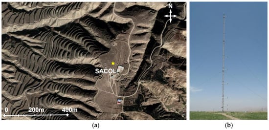
The observations used in this study were collected at the Semi-Arid Climate and Environment Observatory of Lanzhou University (SACOL). The site is located in Gansu Province, China (35°94′N, 104°13′E) at an elevation of 1965.8 m. The region has a semi-arid climate. The surrounding area is characterized by typical Loess Plateau terrain. The surface is dominated by natural grassland with little human disturbance and is representative of the topography and land cover of the semi-arid Loess Plateau. The site location and underlying surface conditions are shown in Figure 1.
Figure 1.
(a) Topography around SACOL obtained from Google Earth. The yellow star marks the location of the observation site. (b) Boundary layer meteorological tower.
SACOL is equipped with multiple ground-based instruments. These instruments provide the three-dimensional structure of the boundary layer and support observations of LLJ occurrence and structure. A 32.5 m meteorological gradient tower is installed at the site, as shown in Figure 1b. Wind speed sensors (014A-L, Met One, Grants Pass, OR, USA), air temperature and humidity sensors (HMP45C-L, Vaisala, Vantaa, Finland), and wind direction sensors (034B-L, Met One) are mounted at 1, 2, 4, 8, 12 and 32 m. These sensors continuously measure near-surface profiles of wind, temperature and humidity.
An eddy-covariance (EC) system is installed at 10 m on the tower. The system consists of a three-dimensional ultrasonic anemometer (CSAT3, Campbell Scientific, Co., Logan, UT, USA) and an open-path infrared gas analyzer (LI-7500, LI-COR Biosciences, Lincoln, NE, USA). The EC system samples three-dimensional wind, temperature and CO2/H2O scalar fluctuations at 10 Hz. The sensor heads are oriented 75° east of north.
A scanning Doppler wind lidar (DWL) is deployed at the base of the tower. The DWL operates in DBS-5 (five beam) mode. It scans in four orthogonal azimuth directions with a fixed elevation angle and includes one vertical beam to obtain radial wind speed from multiple directions. In this experiment, the DWL used an elevation angle of 60°, a range of 103 to 7846 m, and a range resolution of 30 m (about 299 range gates). The single beam temporal resolution was about 6.5 s, and one full scan took about 33 s. This study used horizontal wind speed and wind direction profiles below 2000 m (80 levels in total).
2.2. Multi-Source Fused Low-Level Meteorological Dataset
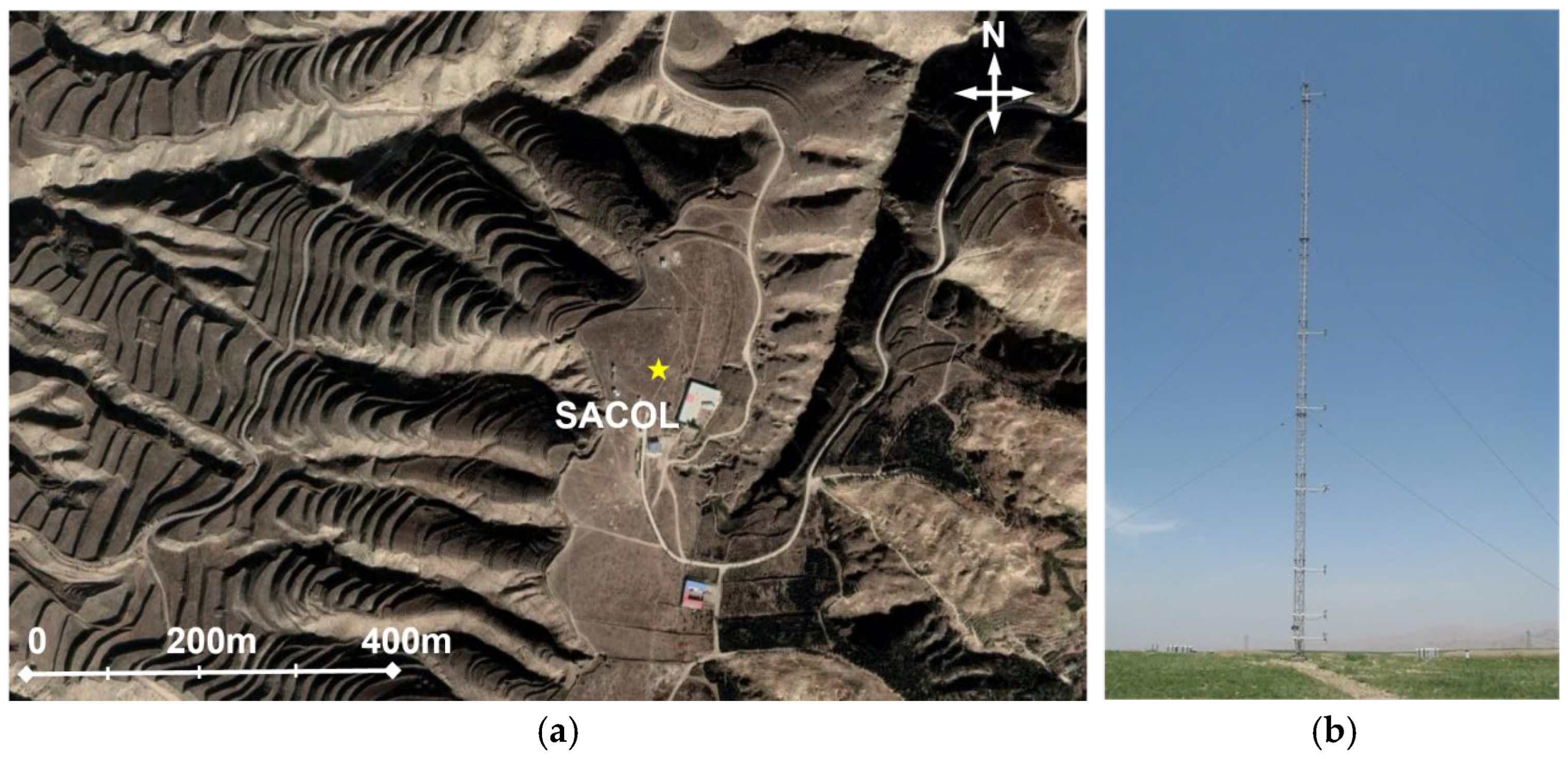
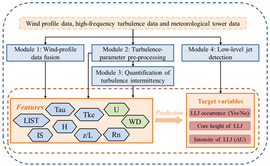
To account for differences in data quality and spatiotemporal resolution among eddy-covariance, tower gradient and Doppler wind lidar observations, four preprocessing modules were designed (Figure 2). A unified multi-source fused dataset of low-level meteorological variables was constructed as follows.
Figure 2.
Flowchart of low-level meteorological data fusion and processing.
(1) Radar tower wind profile fusion: After spike removal and basic quality control, lidar wind profiles and tower wind speed and wind direction data were aligned within a common 30 min time window. Fused 30 min mean wind fields below 2000 m were then obtained. Net radiation (Rn) was directly obtained from the meteorological tower measurements.
(2) Turbulence preprocessing: The EddyPro software (Advanced mode, Version 6.2.1, LI-COR Biosciences, Inc., USA) was used for turbulence quality control and preprocessing, including despiking, double rotation and mean trend removal. The calculation formulas for sensible heat flux (H), turbulent kinetic energy (TKE), the stability parameter (z/L), and momentum flux (Tau) are as follows:
(3) Quantification of turbulence intermittency: Intermittency indices (LIST and IS) were calculated to describe nonstationary and intermittent characteristics.
(4) LLJ identification: Following the LLJ identification method proposed by Bonner [1], LLJ events were automatically detected from the fused wind profiles. The maximum wind speed Umax in the vertical profile of horizontal wind and the minimum adjacent wind speed Umin above Umax were first determined. The wind speed difference was defined as ΔU = Umax − Umin. An LLJ event was identified if a structure with Umax > 10 m/s and ΔU > 3 m/s existed below 2000 m, or if a structure with Umax > 6 m/s and ΔU > 2 m/s existed below 300 m.
Based on these procedures, an integrated feature set was constructed, including wind speed vectors, turbulence fluxes and stability parameters, and turbulence intermittency indices. The LLJ identification module then provided the target variables for machine learning modeling: LLJ occurrence (classification), LLJ core height zmax (m), and LLJ intensity ΔU. This dataset offered a unified and physically interpretable input for the subsequent LLJ-2Stage occurrence detection, height and intensity regression, and SHAP-based identification of dominant controlling factors.
To better represent turbulence intermittency during LLJ formation and evolution, Module 3 used the SMT algorithm to calculate two intermittency indices, LIST and IS [41,42]. Ren et al. [41,42] developed and improved the SMT algorithm based on the Hilbert–Huang transform. The algorithm automatically separates and reconstructs sub-mesoscale motions and turbulent motions for each 30 min window. It yields three-component turbulent fluctuations (Uturb′, Vturb′, Wturb′) and sub-mesoscale fluctuations (Usmeso′, Vsmeso′, Wsmeso′). Turbulent kinetic energy (TKE) and sub-mesoscale kinetic energy (SKE) are then calculated, where SKE represents the kinetic energy of sub-mesoscale motions and TKE represents the kinetic energy of turbulent motions.
On this basis, Ren et al. [41,43] defined two indices to quantify turbulence intermittency: the local intermittent strength of turbulence (LIST) and the intermittency strength (IS). These two indices describe intermittency from the perspectives of turbulent kinetic energy and sub-mesoscale kinetic energy, respectively. The definitions of LIST and IS can be calculated as follows:
The SMT algorithm and the LIST and IS indices have been applied to studies of turbulence intermittency over different underlying surfaces, including homogeneous surfaces [43], arid complex terrain [44,45], polar regions [46] and urban surfaces [43,47].
2.3. Machine Learning Methods and Evaluation Metrics
A two-step modelling strategy was adopted. The first step (classification) determined whether an LLJ event occurred. The second step (regression) predicted the LLJ core height zₘₐₓ(m) and intensity ΔU for the samples with LLJ occurrence.
To evaluate the suitability of machine learning for LLJ prediction, six commonly used algorithms were compared under a unified data splitting and evaluation procedure: LightGBM [48], XGBoost [49], CatBoost [50], k-nearest neighbors (KNN) [51], Balanced Random Forest [52], and ExtraTrees [53]. The models with the best validation performance were selected to construct the two-stage LLJ-2Stage prediction system.
For the classification task, the evaluation metrics were precision, recall, F1-score and PR-AUC. For the regression tasks, the evaluation metrics were the mean absolute error (MAE) and the coefficient of determination (R2). All metrics were computed and analyzed on the independent test set.
Precision is defined as the proportion of true LLJ occurrences among all samples predicted as “occurrence”. Higher precision indicates fewer false alarms. Recall is the proportion of correctly detected LLJ occurrences among all true LLJ samples. Higher recall indicates fewer missed events. The F1-score is the harmonic mean of precision and recall. A higher F1-score indicates better overall classification performance. PR-AUC (average precision, AP) is the area under the precision–recall (PR) curve (range 0–1). A larger PR-AUC indicates stronger overall detection capability.
MAE is the mean absolute difference between predicted and observed values. It reflects the average magnitude of prediction errors; smaller MAE indicates more accurate and robust regression performance. R2 is the fraction of the observed variance explained by the model. It measures the goodness of fit; values closer to 1 indicate higher explanatory power.
2.4. SHAP-Based Interpretability Method
SHAP (Shapley Additive Explanations) is a method that is widely used as a tool for interpreting various machine learning models [54]. The SHAP value (Shapley value) is a way to distribute contributions in team cooperation. For a prediction model and an input feature vector , the SHAP value is the contribution of feature to the prediction, and it is calculated by the following formula:
Here, is the set of features, and is a subset of features that does not contain feature . The function denotes the prediction of a model trained using only the features in subset, and the function denotes the prediction of a model trained using the full feature set. By summing over all possible feature subsets , is obtained. The SHAP value of a feature can be positive or negative. A positive value indicates that this feature increases the prediction, while a negative value indicates that this feature decreases the prediction. At the same time, the magnitude of the absolute value of the SHAP value represents the importance of the feature for the prediction result, and a larger absolute value indicates a stronger influence of the feature.
3. Results
3.1. Characteristics of LLJs over the Loess Plateau Underlying Surface
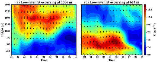
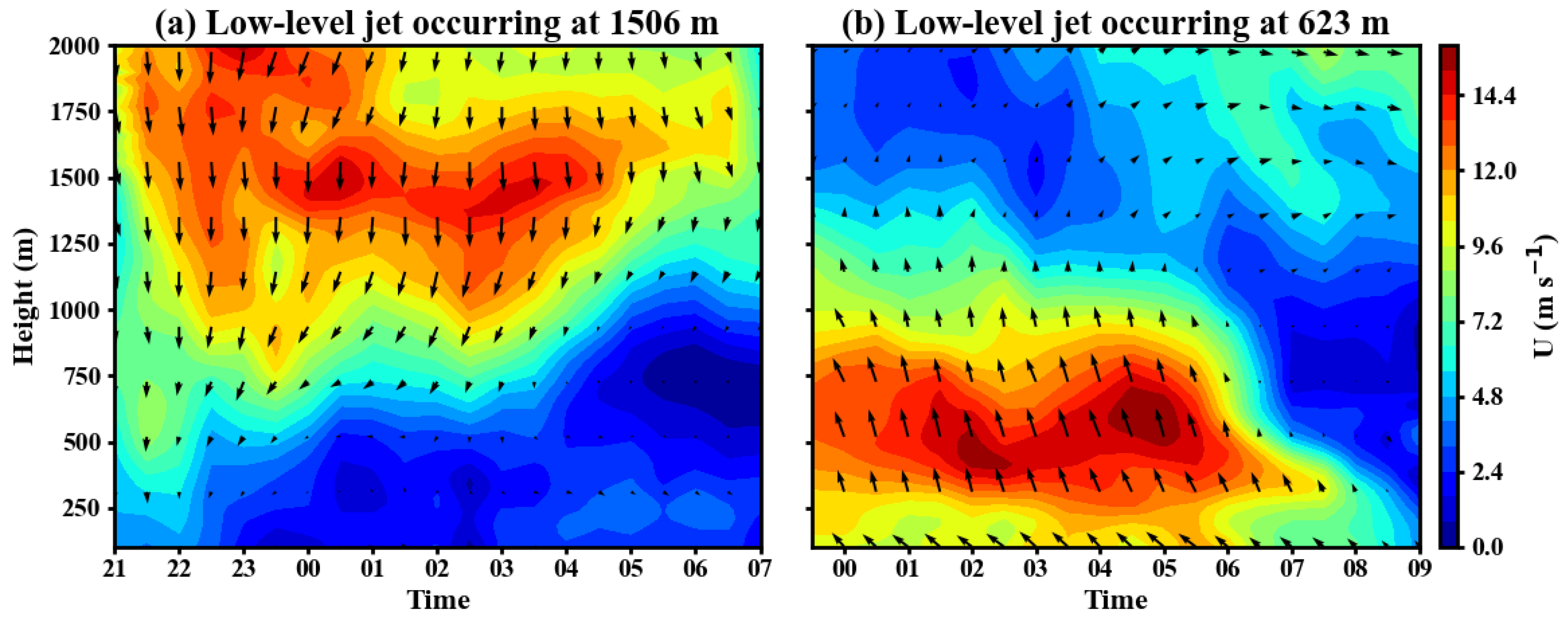
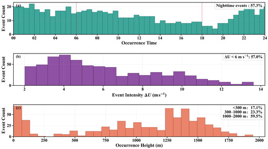
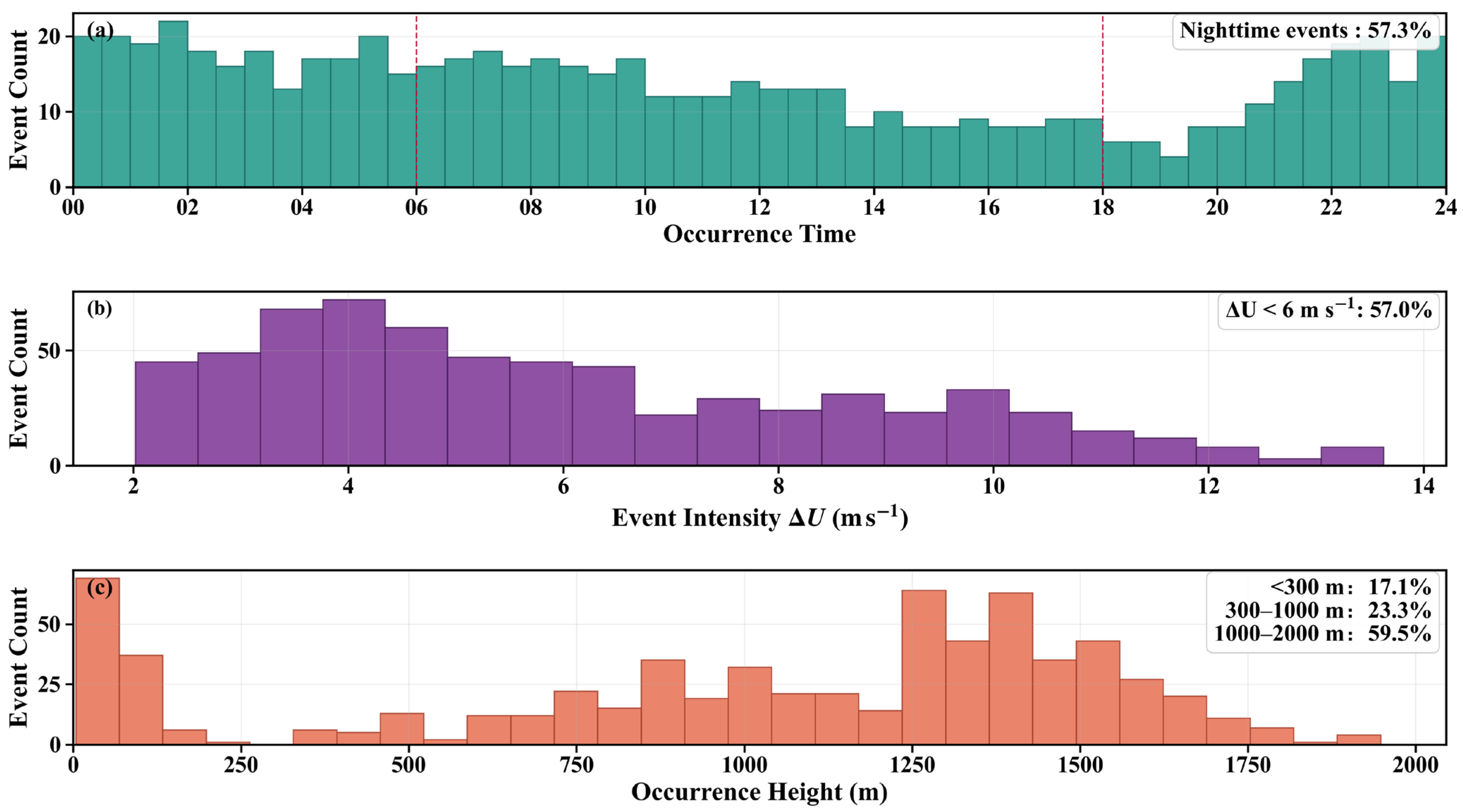
A total of 4204 half hourly samples were obtained at the SACOL site in winter (November and December 2023) and spring (April 2024). A total of 662 LLJ samples were identified, and the occurrence frequency accounted for about 15.75% of all samples. Figure 3 directly shows two identified LLJ cases. The two LLJs show obvious jet cores at 1506 m and 623 m, respectively, and the wind speed above the jet core decreases rapidly, forming a typical nose-shaped profile. The maximum wind speed and its vertical shear both satisfy the LLJ identification criteria used in this study, indicating that the identified cases are consistent with the definition of LLJs. Statistical results show that LLJs over the Loess Plateau occur mainly at night. As shown in Figure 4a, nocturnal LLJs account for about 57.3% of LLJs. In terms of intensity, LLJs over the Loess Plateau are mainly of weak to moderate strength. As shown in Figure 4b, samples with LLJ wind shear ΔU < 6 m/s account for about 57%. In terms of height, as shown in Figure 4c, LLJs are mainly concentrated in the 1000–2000 m layer, accounting for about 59.5% of LLJs.
Figure 3.
Color-shaded plots of LLJ’s horizontal wind speed as a function of time and height. (a) Case on 3 April 2024 at 04:00, with core height 1506 m and ΔU of 11.47 m/s. (b) Case on 12 April 2024 at 04:00, with core height 623 m and ΔU of 6.94 m/s.
Figure 4.
Statistics of LLJ occurrence. (a) Distribution of LLJ occurrence at different times of day with a 30 min interval; higher bars indicate more LLJs at that time. (b) Distribution of LLJ intensity (ΔU). (c) Distribution of LLJ occurrence height.
To assess the regional representativeness of our samples, we compared the above characteristics with the LLJ climatology over China derived from long-term radiosonde observations from 2011 to 2017. Yan et al. [55] reported that LLJs accounted for about 19.4% of the total samples, with pronounced seasonal variability. In particular, the occurrence frequency in Northwestern China was the lowest in winter, and LLJs generally tended to occur at night. They also showed that the jet-core height over China typically ranged from 600 to 1300 m, while plateau regions exhibited higher jet-core heights. In this context, the SACOL LLJs in our study, which were predominantly nocturnal and of weak-to-moderate intensity, are qualitatively consistent with the long-term national statistics. The jet-core heights concentrated around 1000 to 2000 m further reflect the regional feature of an overall upward shift of the jet layer associated with the elevated terrain of the Loess Plateau. It should be emphasized that our samples covered only winter and spring and were based on 30 min data and specific identification criteria. Therefore, a slightly lower occurrence frequency than that reported in multi-year radiosonde climatologies is a reasonable difference arising from the analyzed period and methodological choices, and it does not affect our characterization of LLJ structure and spatiotemporal variability over this region.
3.2. Comparison of LLJ Occurrence Prediction
Given the relatively low proportion of LLJ occurrences in the dataset, the classification task exhibited a significant class imbalance problem. To avoid sampling bias and ensure comparability, stratified random sampling was used in the classification stage to split the data into training and test sets with a ratio of 80% to 20%, while keeping the proportion of LLJ events in each subset consistent with that in the full dataset. In the regression stage, only samples with LLJ occurrence were modeled. Conventional random sampling was applied, with the same 80% and 20% split between the training and test sets. We used a unified configuration across models (500 trees/boosting rounds, depth 10, shrinkage 0.05 for boosting, and five neighbors for kNN). Except for these key settings, other hyperparameters were kept at default values in each library. With this design, we did not perform extensive, model-specific hyperparameter optimization; instead, we report results under the above unified configuration, focusing on the methodological contribution of the proposed two-stage framework.
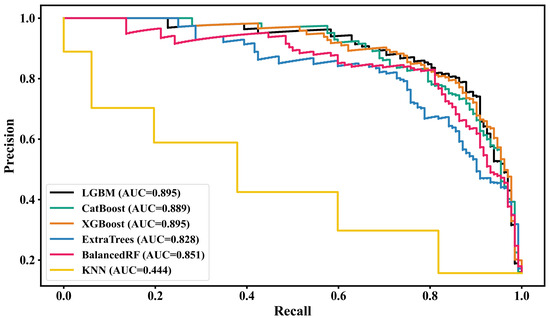
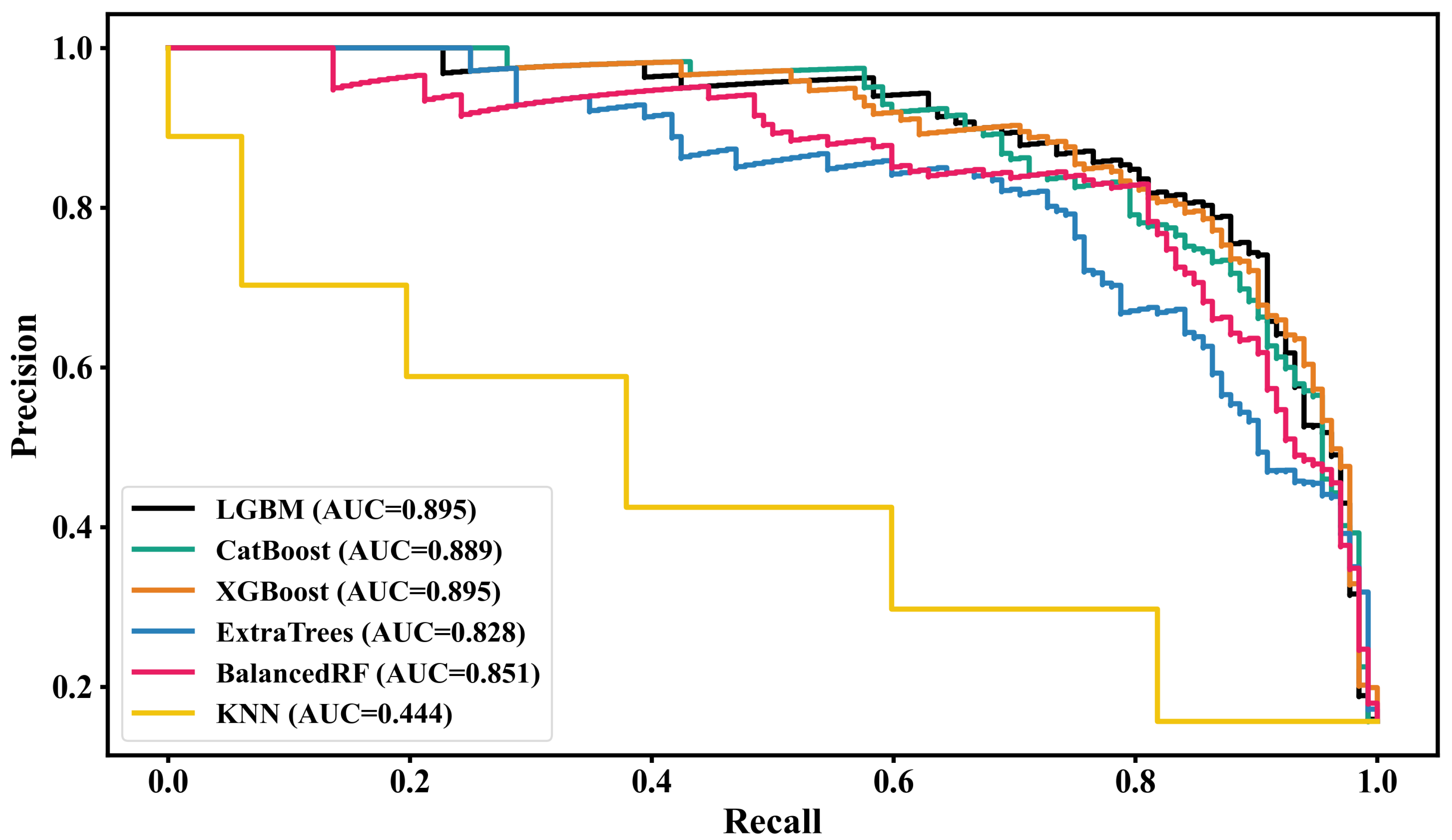
Under a unified data and evaluation setting, the performance of six classification models for LLJ occurrence identification was compared. As shown in Table 1, LGBM showed the best overall performance, with the highest precision of 0.847 and a good recall of 0.795, leading to the highest F1-score of 0.820. This indicates that the model can effectively capture most LLJ occurrences while minimizing false alarms. Operationally, its relatively balanced precision and recall make it a practical baseline for wind energy alerting or low-altitude wind-risk awareness. Compared with LGBM, the F1-scores of XGBoost and CatBoost were 0.816 and 0.798, respectively, and their overall performance was slightly inferior. ExtraTrees attained the highest precision (0.864) among all models, but its recall was much lower (0.530), indicating a conservative behavior that triggered alerts mainly when the signals were very clear, resulting in fewer false alarms but more missed events. Balanced Random Forest achieved the highest recall (0.909) but a lower precision (0.588), reflecting a stronger emphasis on detecting the minority class at the expense of more false alarms, likely due to its class-balancing sampling strategy. KNN performed the worst (F1 = 0.461), mainly because distance-based discrimination becomes less reliable in a high-dimensional feature space, leading to unstable decision boundaries and limited robustness. Overall, these results highlight the advantage of LGBM in balancing precision and recall under nonlinear relationships and class-imbalanced conditions.
Table 1.
Performance comparison of different machine learning models in the LLJ occurrence classification task (precision, recall, F1-score).
The PR curves in Figure 5 further support the above conclusions. The curves of LGBM and XGBoost maintain higher precision in the medium to high recall range and are located above those of the other models. CatBoost ranks second: it is slightly better in the high precision region but drops markedly in the high recall region. ExtraTrees mainly occupies the region with high precision and low recall, and its precision decreases rapidly as recall increases. BalancedRF extends obviously into the very high recall region but with a marked drop in precision. The KNN curve declines significantly overall. The shapes of the curves are basically consistent with the ordering of the numerical scores in Table 1, indicating that LGBM maintains better classification performance across different thresholds. Overall, the LGBM model had the highest F1-score and a stable PR-curve shape, balancing high precision and high recall and enabling effective prediction of LLJ occurrence.
Figure 5.
Comparison of precision–recall (PR) curves of different machine learning models for low-level jet (LLJ) occurrence identification. The horizontal axis is recall, which denotes the proportion of LLJ events that are correctly identified among all true LLJ occurrences. The vertical axis is precision, which denotes the proportion of truly LLJ samples among those classified as LLJ by the model. Each curve corresponds to one classification model. The value in brackets in the legend is the area under the PR curve (AUC) on the test set; a larger value indicates better overall identification performance. It can be seen that the curves of LGBM, CatBoost and XGBoost are closer to the upper right corner, indicating better performance than ExtraTrees and BalancedRF, while KNN performs the worst.
Building on the PR-curve comparison, we additionally report precision and recall at two representative probability thresholds, the default threshold of 0.5 and the threshold that maximizes F1, to provide concrete operating points. At the default threshold of 0.5, LGBM and XGBoost remained well balanced, with LGBM achieving a precision of 0.847 and a recall of 0.795 and XGBoost achieving a precision of 0.807 and a recall of 0.826. At the F1-optimal threshold, LGBM attained the highest F1 of 0.832 at a threshold of 0.223 with a precision of 0.803 and a recall of 0.864, while XGBoost yielded F1 0.825 at a threshold of 0.422 with a precision of 0.796 and a recall of 0.856. CatBoost reached its best balance at a higher threshold of 0.560, maintaining a precision of 0.827 with a recall of 0.795, indicating a more conservative operating point. From an operational perspective, under a higher threshold, CatBoost is a suitable example for wind energy applications that prefer conservative alerting, whereas LGBM under its F1-optimal threshold is a suitable example for safety-oriented aviation monitoring that prioritizes higher event-detection sensitivity.
3.3. Comparison of LLJ Height and Intensity Predictions
The height of LLJs (jet core height) and their intensity (represented by the wind shear ΔU) are key physical properties for evaluating their potential hazard. They are also core variables in flight safety assurance and boundary layer dynamics research. Accurate prediction of LLJ height and intensity is therefore of great importance. On the basis of the classification module, a second-stage regression module was introduced, and prediction modelling was carried out for samples with LLJ occurrence, in order to avoid the influence of non-LLJ samples on the regression results. The performance of the six selected machine learning models in regression prediction was evaluated and compared.
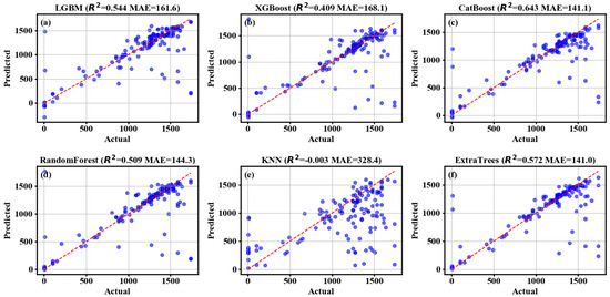
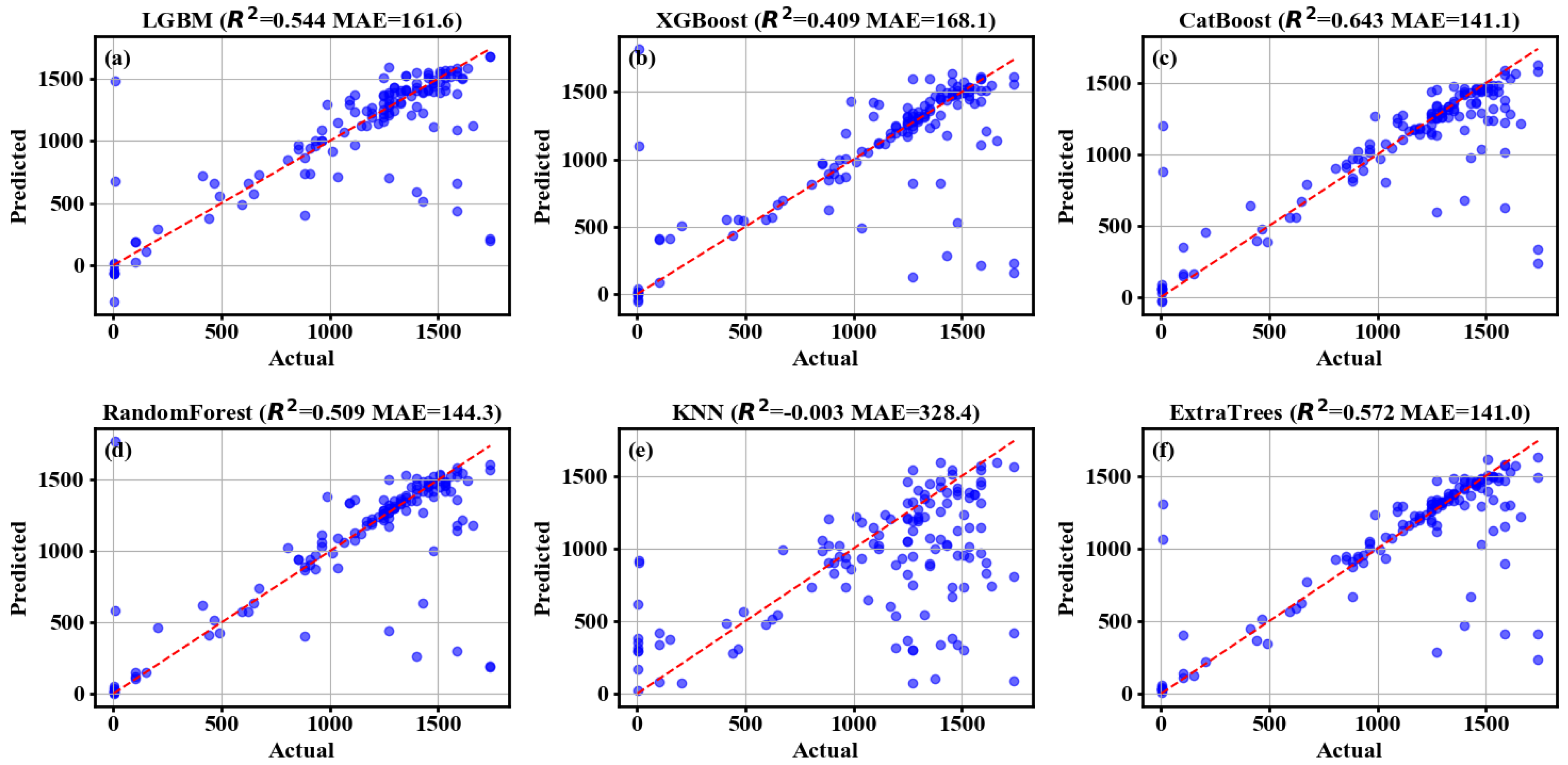
For the LLJ height prediction task (as shown in Figure 6), the performance differences among the models were relatively small. The CatBoost model performed best, with a height MAE of 141.1 m and R2 of 0.643. In contrast, although ExtraTrees had a slightly better MAE of 141.0 m, its R2 was only 0.572, indicating lower prediction accuracy. The errors of LGBM and RandomForest were clearly larger, with R2 values of 0.544 and 0.509, and their accuracy was slightly inferior to that of ExtraTrees and CatBoost, reaching only a moderate level. The performance of XGBoost was average, with an MAE of 168.1 m and R2 of 0.409, indicating relatively poor prediction skill. The instance-based KNN model performed the worst and could no longer effectively learn the complex mapping between jet height and its influencing factors.
Figure 6.
Scatter plots of the relationship between predicted and observed LLJ height (height, unit: m) for the six machine learning models. Panels (a–f) correspond to LGBM, XGBoost, CatBoost, RandomForest, KNN and ExtraTrees, respectively, and a 1:1 reference line is used as the baseline.
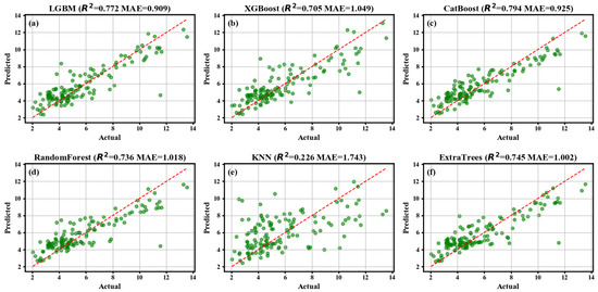
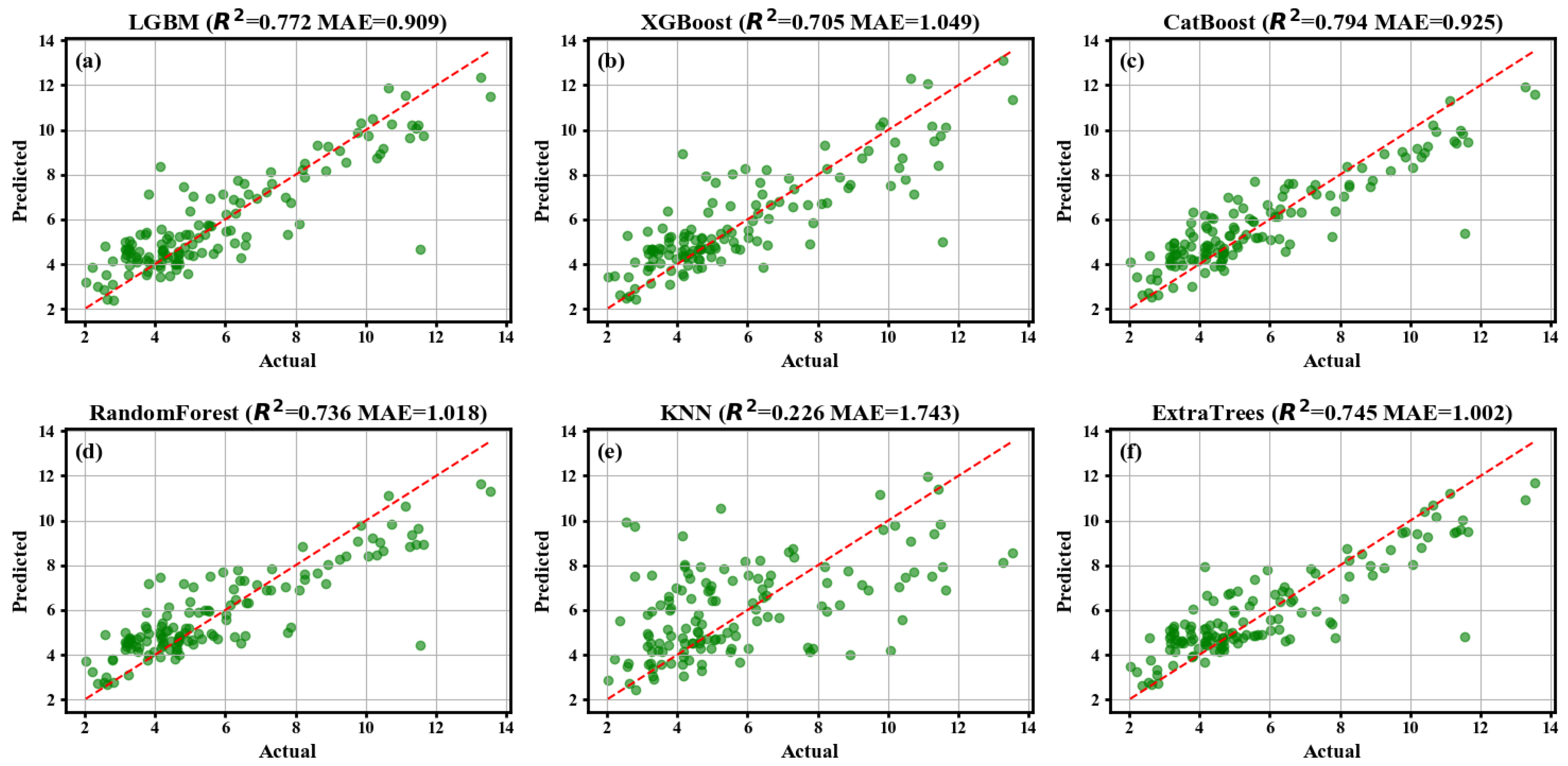
For LLJ intensity prediction (as shown in Figure 7), there were obvious performance differences among the models. The CatBoost model showed the highest accuracy, with an intensity MAE of 0.925 m/s and R2 of 0.794. LGBM and ExtraTrees ranked second, with R2 values of 0.772 and 0.745 and MAE values of 0.909 m/s and 1.002 m/s, respectively, and their prediction performance was slightly inferior to CatBoost. The errors of RandomForest and XGBoost were relatively larger, with R2 decreasing to 0.736 and 0.705, respectively. KNN performed the worst, with an intensity MAE of 1.743 m/s and R2 of only 0.226. Overall, CatBoost achieved the best performance in intensity prediction, whereas the prediction accuracy of the other models was relatively low.
Figure 7.
Scatter plots of the relationship between predicted and observed LLJ intensity (ΔU, unit: m/s) for the six machine learning models. Panels (a–f) correspond to LGBM, XGBoost, CatBoost, RandomForest, KNN and ExtraTrees, respectively, and a 1:1 reference line is used as the baseline.
3.4. LLJ-2Stage Prediction System Architecture and Results
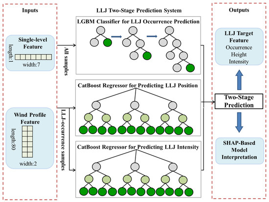
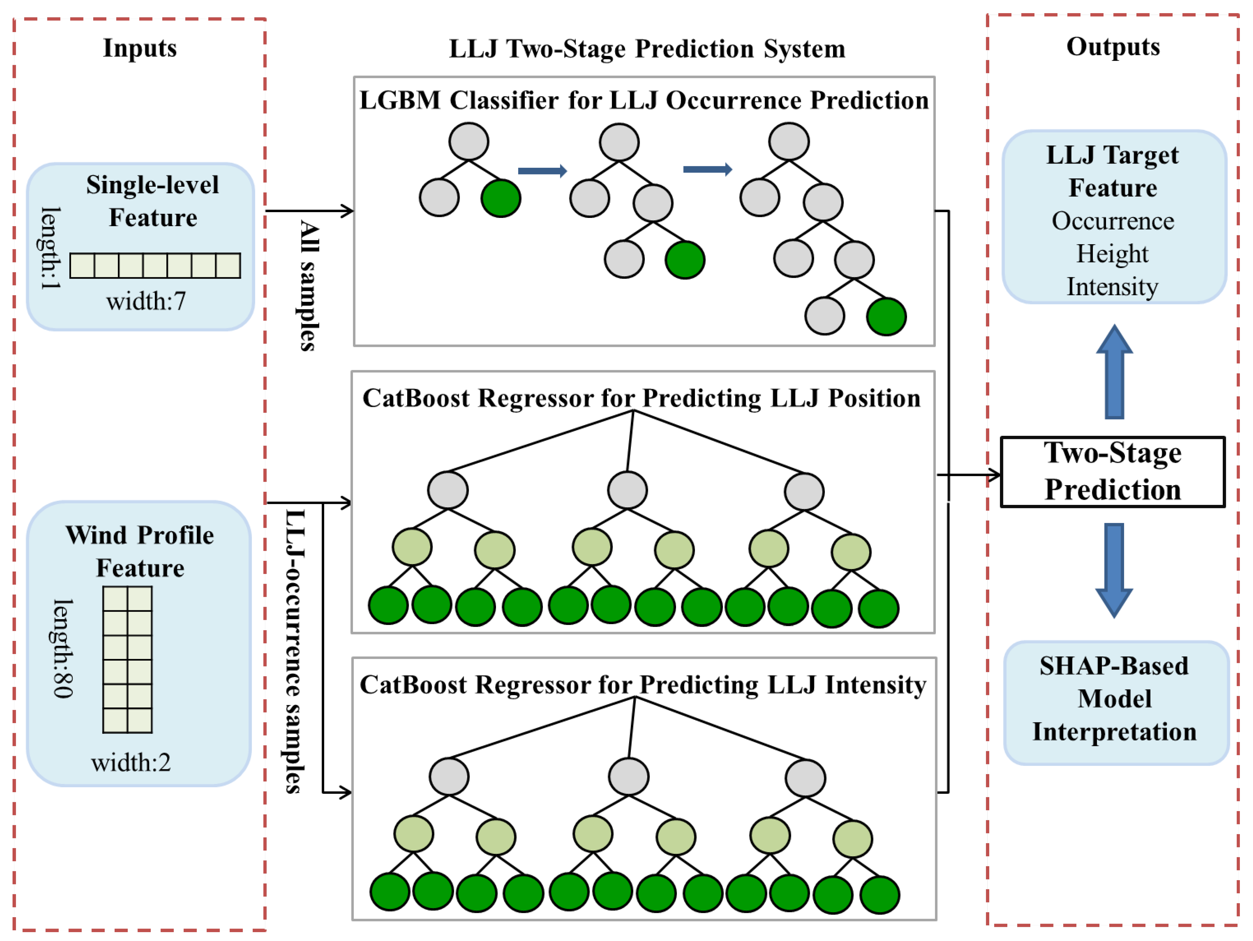
Based on the comparison results of the six machine learning methods, this study constructed an LLJ-2Stage prediction system, as shown in Figure 8. In the first stage of the LLJ-2Stage model, it is determined whether an LLJ event exists at the target time. In the second stage, the LLJ core height and LLJ intensity (ΔU) are predicted separately. Different models were selected for different prediction targets. LLJ occurrence prediction used the LightGBM model, which had the highest F1-score (0.820). The height prediction task used the CatBoost model (R2 = 0.643, MAE = 141.1 m). The intensity prediction task also used the CatBoost model (R2 = 0.794, MAE = 0.925 m/s). In this way, the advantages of each algorithm in its corresponding task were fully utilized, and the reliability of predicting key LLJ characteristics was improved.
Figure 8.
Flowchart of the LLJ-2Stage prediction system.
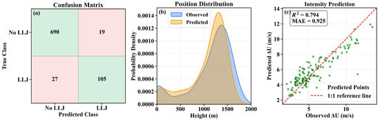
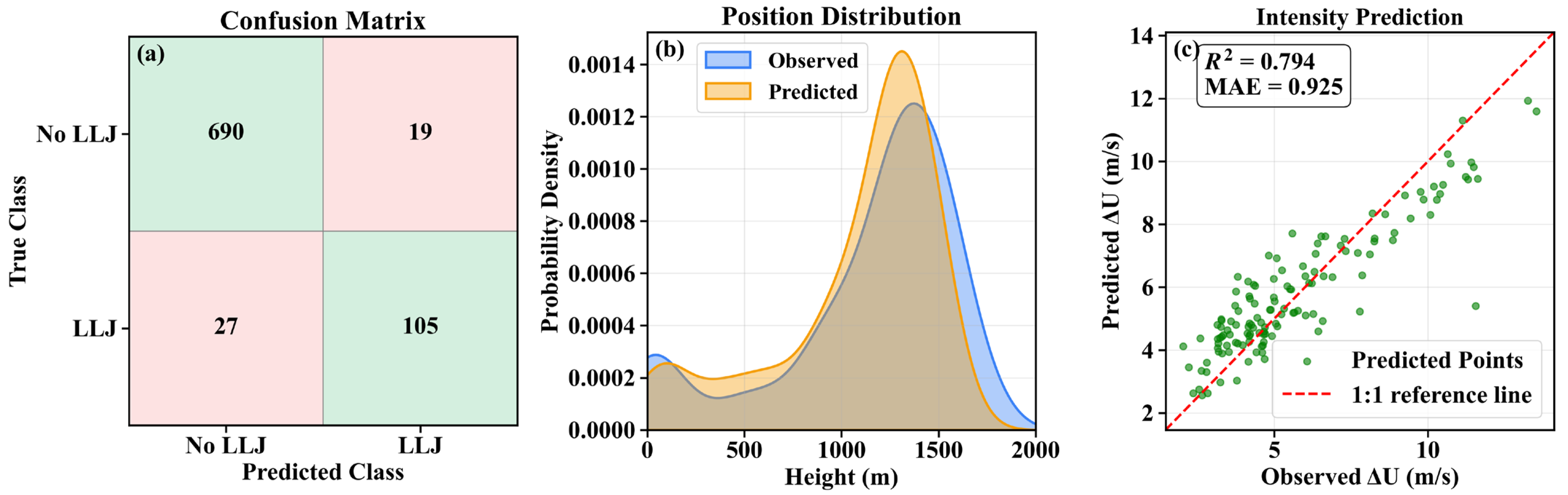
To provide a comprehensive and intuitive description of the LLJ-2Stage model, Figure 9 shows the overall performance of the LLJ-2Stage model. As shown in Figure 9a, the model can accurately identify the sample categories in most cases. Our occurrence identification model achieved Precision = 0.847, Recall = 0.795, F1 = 0.820. Compared with the NN-based LLJ alerting approach of Kwong et al. [28], which reported a correct prediction rate of 72% and a false-alarm rate of 27%, our classifier yielded higher overall performance and a lower false-alarm tendency under our evaluation metrics. For the minority class of LLJ occurrence, the model still maintained a high identification ability. For LLJ height prediction, the correlation coefficient was R2 = 0.643. As shown in Figure 9b, the model predictions matched the observed distribution very well in the overall trend and could accurately reproduce the main height range of LLJ occurrence. As seen in Figure 9c, the scatter points are concentrated near the regression fitting line and overall show a linear correlation. The correlation coefficient was R2 = 0.794, the MAE was 0.925 m/s, and the error was within a reasonable range. To highlight the added value of multi-source data fusion, we further used the LLJ two-stage model to compare performance using wind-profile remote-sensing features only versus using the fused feature set adopted in this study (figure omitted). The results showed that the model trained with the fused dataset, which additionally included flux variables, stability parameters, and intermittency indices, achieved similar performance for LLJ occurrence prediction to the configuration using wind-profile features alone. For core-height prediction, the fused-feature configuration performed noticeably better below 1000 m, whereas no clear improvement was found for LLJ cores above 1000 m. This suggests that turbulence-related information derived mainly from near-surface observations provides limited constraints on higher-elevation jets. For intensity prediction, the fused-feature configuration yielded better performance, with R2 increasing from 0.766 to 0.794. In summary, the model shows high accuracy and stability in predicting LLJ occurrence and structural evolution and has good application prospects.
Figure 9.
Overall performance of the LLJ-2Stage model. (a) Confusion matrix obtained from the classification part of the LLJ-2Stage model. (b) Kernel density estimation (KDE) of observed and predicted LLJ heights. (c) Scatter plot of observed and predicted LLJ intensity (ΔU) (R2 = 0.794, MAE = 0.925 m/s); the red dashed line is the ideal 1:1 reference line.
3.5. Machine Learning Interpretability Analysis
Although machine learning models show excellent performance in LLJ identification and feature prediction, their black-box nature limits the physical interpretation of the basis for model decisions. In order to determine the main driving factors that affect LLJ occurrence and structural evolution and to examine the consistency between these driving factors and theoretical understanding, the SHAP (Shapley Additive Explanations) method was introduced in this study to visualize the important input features of the model and their directions of influence.
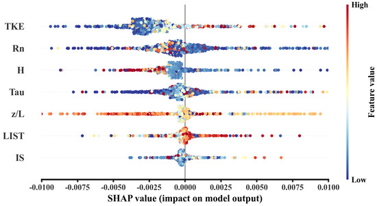
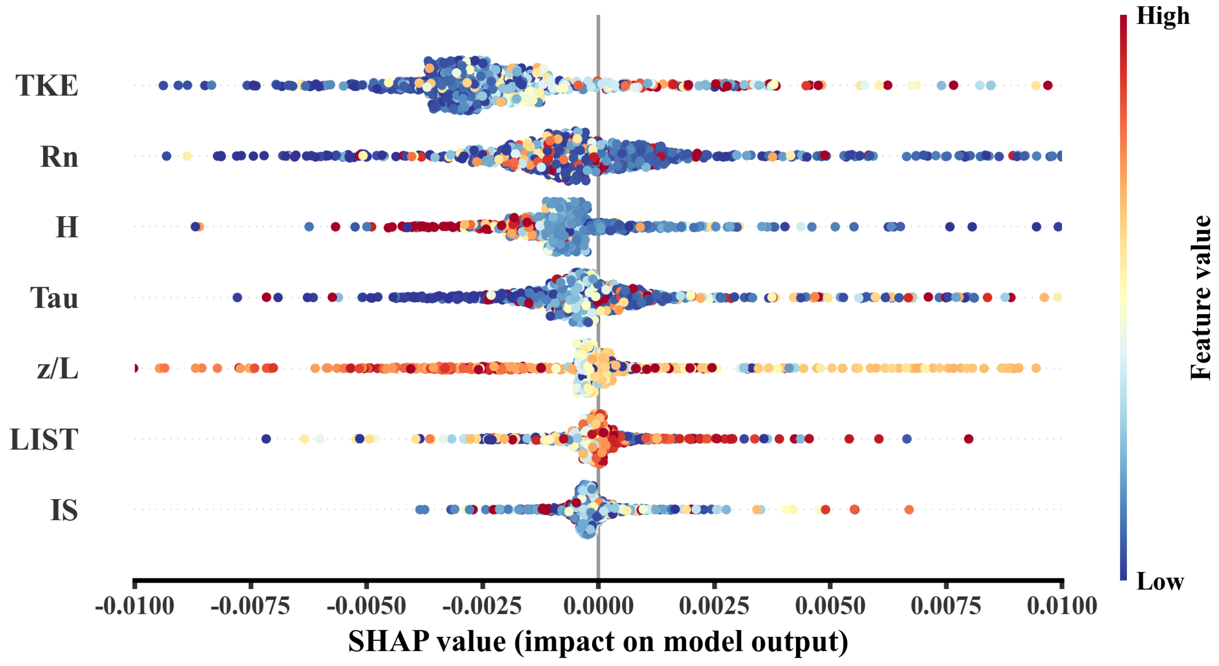
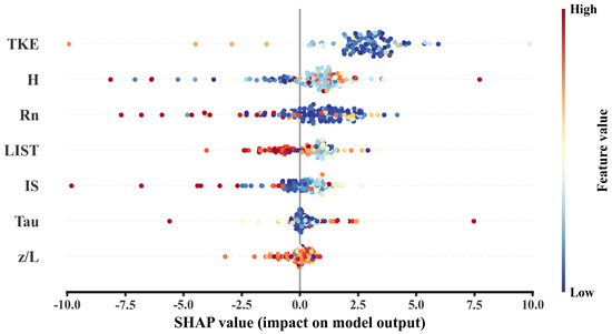
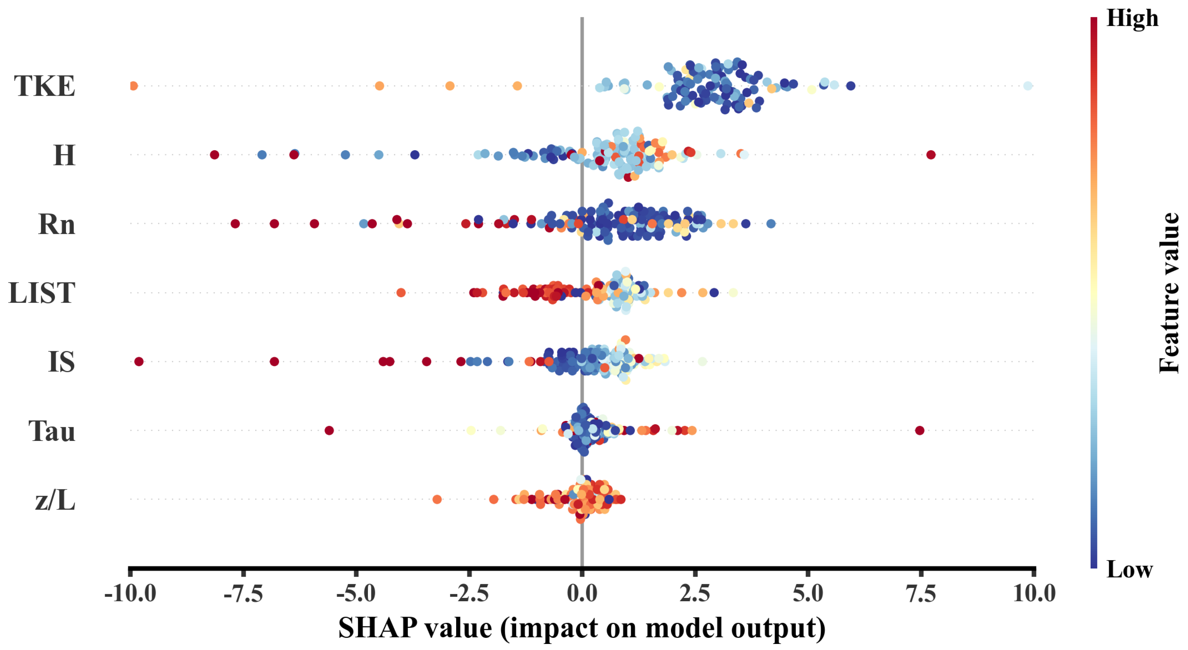
The analysis showed that, in the classification task of whether a jet occurs (Figure 10), the variable on which the model relied most when judging the occurrence of LLJs was turbulent kinetic energy TKE, followed by net radiation Rn and sensible heat flux H. TKE had the largest impact on the classification results. Samples with higher TKE often corresponded to positive SHAP contributions to the LLJ-occurrence prediction, indicating that enhanced near-surface turbulence was correlated with a higher model-predicted probability of LLJ occurrence. After TKE, the thermal factor that the model valued most was net radiation Rn. Under low Rn conditions, the corresponding SHAP values for the model output were mainly positive, indicating that LLJs were more easily triggered, which is consistent with the mechanism that nocturnal stable stratification induced by radiative cooling favors inertial oscillations and jet formation. Sensible heat flux H ranked third. Its SHAP distribution was overall similar to that of Rn: low H or downward sensible heat flux corresponded to positive contributions, reflecting that surface cooling and strengthened stable stratification are more favorable for the generation of LLJs. LIST and IS ranked sixth and seventh in relative importance. Low LIST produced a certain positive contribution to the model output, which is consistent with boundary layer observations that turbulent burst periods are prone to be accompanied by sudden jets. This indicates that, after TKE, fluxes and z/L have already characterized the main turbulence background, the additional intermittency information has a relatively weak influence on the judgment of LLJ occurrence.
Figure 10.
Scatter plots of SHAP-based feature importance for LLJ occurrence prediction.
In the prediction task of jet occurrence height, the most important feature in the model was turbulent kinetic energy TKE. Figure 11 shows that samples with high TKE make positive contributions to the predicted height, indicating that enhanced near-surface turbulence tends to raise the jet core height. Sensible heat flux H ranked second. When H was close to zero, the SHAP values for height prediction were relatively small; negative H or very low H corresponded to obvious negative contributions, indicating that stronger surface cooling favors a lower jet core. Net radiation Rn was the third most important feature. Its SHAP distribution showed that moderate Rn corresponded to relatively large positive contributions to the predicted height, whereas very low or very high Rn values corresponded to smaller or even negative contributions. This suggests that when radiative forcing is not extremely weak or extremely strong, LLJs are more likely to appear at higher levels. LIST and IS ranked fourth and fifth in relative importance. This suggests that the intermittency indices provide valuable supplementary information for locating the LLJ core height. Specifically, higher LIST values were more frequently associated with negative SHAP contributions, implying a tendency toward a lower predicted core height under strongly intermittent conditions, whereas lower intermittency tended to contribute in weakly positive way to the predicted height. Overall, in this task, the model mainly relied on TKE, Rn and H to capture variations in LLJ height, while the intermittency indices played an auxiliary role.
Figure 11.
Scatter plots of SHAP-based feature importance for LLJ height prediction.
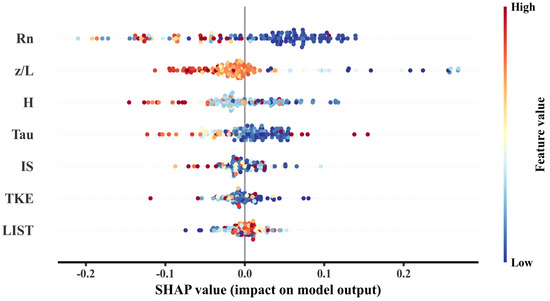
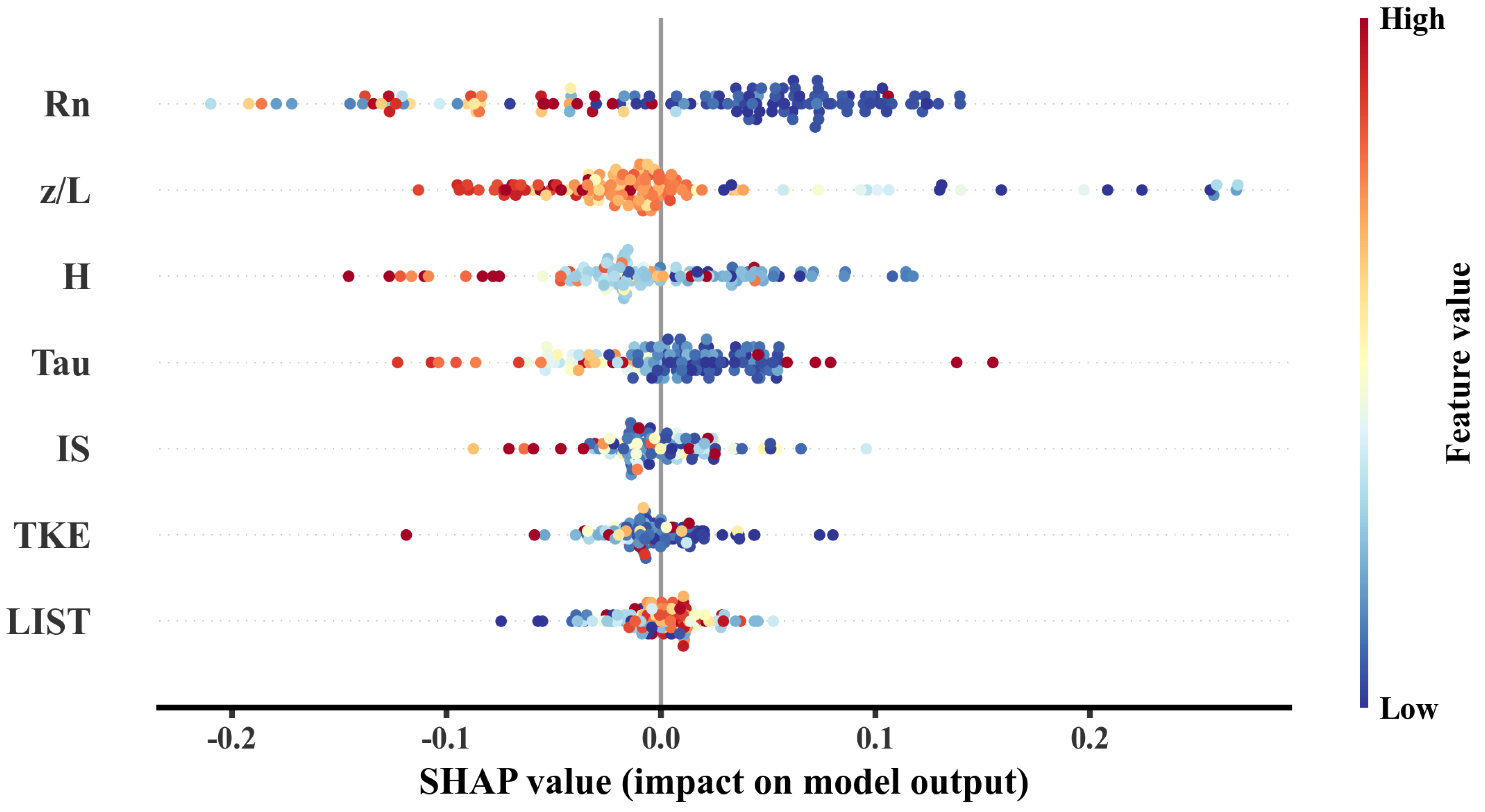
In the prediction task of jet intensity (ΔU) (Figure 12), the feature that the model valued most was net radiation Rn. Its SHAP distribution showed that samples with high Rn were mainly concentrated near zero or negative SHAP values, indicating that strong radiative forcing tends to reduce the predicted jet intensity, whereas low Rn conditions correspond to positive SHAP contributions and favor stronger jets. The second most important feature was the stability parameter z/L. When z/L was close to neutral, the corresponding SHAP values of ΔU were relatively small; as z/L became more positive, the SHAP values showed an overall increasing trend, which means that strongly stable stratification is more conducive to the formation of large ΔU. Sensible heat flux H ranked third. Negative H or small H corresponded to positive SHAP values of ΔU, while large positive H corresponded to negative SHAP values, reflecting that downward sensible heat flux and near-surface cooling favor a stronger jet. In comparison, IS ranked fifth in importance, and LIST ranked seventh. Their SHAP values were generally closer to zero with a smaller overall spread, suggesting that their contributions to jet intensity prediction are relatively limited. Nevertheless, IS and LIST still exhibited discernible positive and negative variations, indicating that information on nonstationary and intermittent turbulence can provide supplementary cues for locating the jet intensity, with a role that appears more consistent with subtle modulation on top of the dominant thermodynamic and stability background. Turbulent kinetic energy TKE and turbulent-momentum-flux-related quantities also contributed to the ΔU prediction, but their feature importance rankings were lower, and the additional information that they provided was limited. Overall, in the ΔU prediction, the model mainly relied on Rn, z/L and H to capture changes in LLJ intensity, with turbulence momentum and intermittency indices playing auxiliary corrective roles.
Figure 12.
Scatter plots of SHAP-based feature importance for LLJ intensity prediction.
Combining the results of the three SHAP plots, it can be seen that, under the current feature and sample configuration, the model mainly relies on turbulent kinetic energy TKE, net radiation Rn and sensible heat flux H when judging whether an LLJ occurs. When near-surface turbulence is strong and radiative cooling is enhanced, LLJs are more likely to be judged as occurring. In the height prediction, the model mainly relies on TKE, Rn and H to capture changes in LLJ height, with intermittency indices playing an auxiliary role; in the ΔU prediction, the model mainly relies on Rn, z/L and H to capture changes in LLJ intensity. The intensity of turbulence intermittency provides valuable supplementary information for locating the LLJ core height.
3.6. Temporal Evolution of Key Meteorological Factors Influencing LLJs
While the SHAP analysis above identifies the key predictors and their statistical contributions to the model decisions, it does not, by itself, provide a process-oriented view of how the boundary layer evolves during individual LLJ events. To complement the model interpretation and to strengthen the physical perspective, we further present representative nocturnal LLJ cases and examine the temporal evolution of key variables before, during, and after the events. This case-based analysis helps connect the SHAP-identified predictors to physically interpretable boundary layer processes associated with LLJ onset, maintenance, and decay.
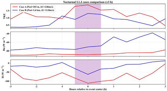
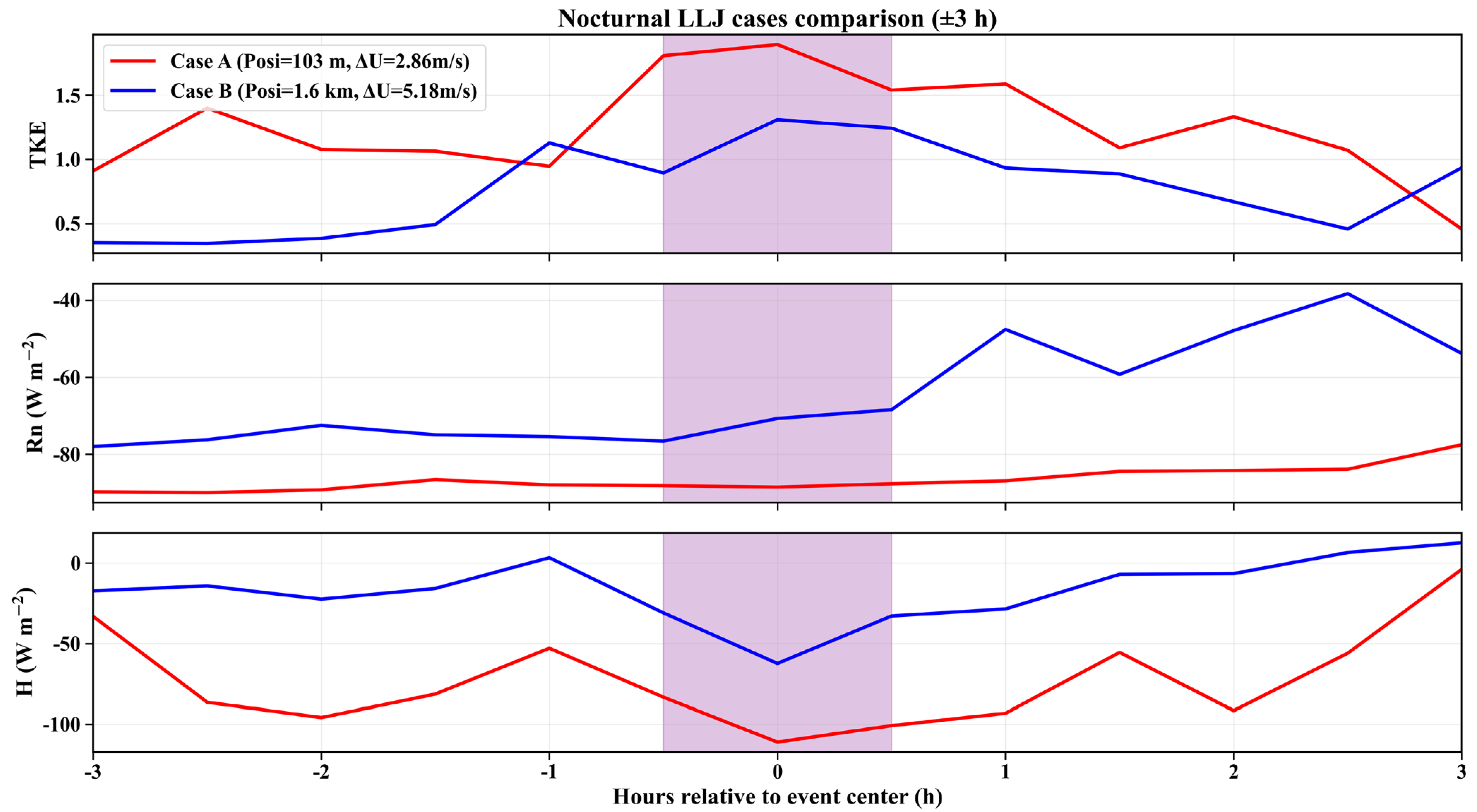
Based on the SHAP interpretability analysis of the classification model, turbulent kinetic energy (TKE), net radiation (Rn), and sensible heat flux (H) make the largest contributions to discriminating whether an LLJ occurs. These variables represent key physical processes, including turbulence intensity, nocturnal radiative cooling, and near-surface thermal exchange, respectively. Therefore, we selected TKE, Rn, and H as the core variables for the case analysis to characterize the evolution of the physical environment before, during, and after LLJ events. Two representative LLJ cases were chosen: Case A was a shallow and relatively weak LLJ with a jet-core height of about 103 m and an intensity of ΔU ≈ 2.86 m/s, occurring during 22:00–23:00 on 8 December 2023; Case B was an elevated and strong LLJ with a jet-core height of about 1.6 km and an intensity of ΔU ≈ 4.63 m/s, occurring during 21:00–22:00 on 10 November 2024. Both cases occurred at night and represent typical nocturnal LLJ structures near the surface and aloft, respectively, thereby capturing representative contrasts across different core-height and intensity regimes. For comparison, Figure 13 is centered on the event midpoint (set to zero time) and shows the evolution of TKE, Rn, and H within a ±3 h window, with the LLJ period shaded.
Figure 13.
Temporal evolution of turbulent kinetic energy (TKE), net radiation (Rn), and sensible heat flux (H) for two nocturnal LLJ cases within ±3 h relative to the event center (0 h). Case A and Case B are shown by the red and blue lines. The purple shaded area denotes the identified LLJ period.
The comparison indicates that both cases occur under a typical nocturnal background within the event window. Net radiation remains negative throughout (Rn < 0), indicating persistent radiative cooling, while sensible heat flux is mostly negative or close to zero (H ≤ 0), suggesting a near-surface stable stratification. This behavior is consistent with the SHAP-indicated influence directions in Section 3.5, namely, that higher TKE and lower Rn and H are often associated with positive contributions to the model-predicted probability of LLJ occurrence. Meanwhile, during the LLJ period, both cases show a consistent near-surface signal, with enhanced TKE and reduced H, followed by a gradual return toward the pre-event level after the LLJ ends, whereas Rn continues to remain low.
4. Discussion
In this section, we first clarify the incremental contributions and added value of the proposed data-fusion strategy and the two-stage machine learning prediction system relative to existing LLJ studies. We then discuss the limitations of the present work and finally provide an outlook on future research directions.
From a remote-sensing perspective, ground-based Doppler wind lidars and wind profiler radars can depict boundary layer wind-field structures with high temporal continuity and fine vertical resolution, making them key data sources for identifying and characterizing LLJs. Many previous studies have used continuous wind-profile information from Doppler wind lidars and other remote-sensing instruments to detect LLJs and to describe their occurrence statistics and evolution. However, under nonstationary and intermittent boundary layer conditions, relying on wind-profile features alone is often insufficient to fully represent the impacts of turbulence processes and the stability background on LLJ formation, maintenance, and abrupt changes. The main value of this study lies in combining remote-sensing wind-profile information with eddy-covariance turbulence statistics, stability parameters, and turbulence intermittency indices to construct a fused multi-source feature set. With this feature set, we developed a two-stage machine learning framework that enables more accurate prediction of LLJ occurrence and quantitative estimation of core height and intensity. We further applied SHAP-based interpretability analysis to identify the dominant controlling factors and to examine their consistency with the underlying physical mechanisms, thereby highlighting the added value of fusing remote-sensing wind profiles with turbulence-related observations for LLJ prediction and interpretation.
Nevertheless, this study has limitations and a clearly defined scope of applicability. First, the dataset was from a single site, SACOL, and was mainly limited to a few months in winter and spring; therefore, the present work should be regarded as a case study for the Loess Plateau under winter and spring conditions. This design is helpful for validating the proposed framework using a relatively complete observational suite, but it also implies that regional representativeness and seasonal applicability may be influenced by differences in surface properties, terrain elevation, and large-scale circulation backgrounds. Meanwhile, in Section 3.1, we compared the key LLJ statistics identified at SACOL with radiosonde-based climatological statistics over China, showing overall consistency in nocturnal dominance, occurrence frequency, and jet core height distributions. This comparison supports the reasonableness of our LLJ samples to some extent; however, it remains a statistical consistency check, and the transfer performance of the model across regions, seasons, and observing systems still needs independent validation using multiple sites and multi-season datasets.
Beyond spatiotemporal sampling, LLJ identification and statistics are also constrained by the vertical coverage and resolution of the observing system. The Doppler wind lidar used in this study provided wind profile coverage from 103 to 7846 m and had a minimum effective detection height; therefore, ultra LLJs with cores below 103 m may be missed. To mitigate this issue, we fused wind speed and wind direction measurements from the 32.5 m gradient tower with the lidar wind profiles to partially compensate for the lack of observations below 103 m. However, an observational gap remains between 32 and 103 m, and jets with cores in this layer may not be captured, which could lead to an underestimation of ultra LLJ occurrence and a slight upward bias in the estimated core height statistics. Accordingly, our conclusions mainly apply to LLJs within the current observational height range. When applying the approach to other observing systems or environments, the identification thresholds and feature construction should be adapted and reassessed according to the minimum detection height and low-level coverage of the target system. In the future, additional observations that fill the near-surface gap would help reduce potential systematic impacts associated with missed ultra LLJs.
In addition, turbulence information in this study was mainly derived from near-surface eddy-covariance observations, reflecting a common challenge in boundary layer meteorology: how to effectively characterize and predict high altitude phenomena across the atmospheric column based on surface or lower-level measurements. Near-surface stability, turbulence intensity, and intermittency can affect LLJ formation and maintenance through mechanisms such as turbulent mixing and downward momentum transport; thus, these quantities provide physically meaningful predictors in a statistical sense and form an important basis for the physical insights offered by the proposed data fusion strategy and interpretability analysis. However, it should be acknowledged that near-surface turbulence information alone may be insufficient to represent LLJ types that are more strongly controlled by processes aloft or synoptic scale forcing, which can limit model generalization and forecasting robustness under complex weather systems. Therefore, at the current stage, the proposed framework is more suitable for LLJ scenarios dominated by local boundary layer processes and surface influences. In the future, incorporating information such as synoptic scale circulation backgrounds and mesoscale environmental fields into the feature set could further enhance the model’s generalization capability and forecasting robustness under complex weather systems.
5. Conclusions
Low-level jets (LLJs) are common, strong wind structures in the atmospheric boundary layer. They have important impacts on flight safety, wind energy utilization and pollutant dispersion. In view of the limitations caused by LLJ–turbulence two-way feedback, intermittency and observational constraints, this study used multi-source observations from the Semi-Arid Climate and Environment Observatory of Lanzhou University (SACOL) over the Loess Plateau. Four processing modules were designed: multi-source data fusion, turbulence preprocessing, turbulence intermittency and LLJ identification. On this basis, a comprehensive feature system suitable for analyzing complex LLJ processes that are nonstationary, nonlinear and intermittent was constructed. The system included wind speed vectors, turbulent fluxes and stability parameters, and turbulence intermittency indices.
Six commonly used machine learning models were compared. LightGBM was selected as the best model for LLJ occurrence prediction. CatBoost was selected as the best model for LLJ height prediction and LLJ intensity prediction. On this basis, an LLJ-2Stage prediction system was constructed. In the first stage, LightGBM was used to determine whether an LLJ occurred, and stable occurrence identification performance was obtained (F1 = 0.820). In the second stage, CatBoost was applied to samples with LLJ occurrence to predict LLJ height and LLJ intensity. This realized a complete prediction from LLJ occurrence to the characterization of height and intensity. The overall errors of the model were within a reasonable range, and the scatter plots showed good agreement between predicted and observed values. These results demonstrate that the system can meet the requirements for predicting LLJ occurrence and, after LLJ onset, predicting LLJ height and intensity.
Finally, the SHAP method was used for the interpretability analysis. The results revealed the effects of different features on LLJs. Under the current feature and sample configuration, when determining whether an LLJ occurred, the model mainly relied on turbulent kinetic energy (TKE), net radiation (Rn) and sensible heat flux (H). When predicting LLJ height, the model mainly relied on TKE, Rn and H to capture changes in LLJ height. When predicting ΔU, the model mainly relied on Rn, z/L and H to capture changes in LLJ intensity. The intensity of turbulence intermittency provided valuable supplementary information for locating the LLJ core height. Beyond the global SHAP-based interpretation, the case-based analysis provided a process-oriented perspective on boundary layer evolution during LLJ events. Specifically, during the LLJ period, both cases showed a consistent near-surface signal with enhanced TKE and reduced H, followed by a gradual return toward the pre-event level after the LLJ ended, whereas Rn continued to remain low, supporting the physical consistency of the identified predictors.
Author Contributions
Conceptualization, Y.R. and H.Z.; methodology, M.C.; software, M.C.; validation, M.C.; formal analysis, M.C. and Y.R.; investigation, M.C., J.L., X.C. and P.T.; resources, Y.R. and L.Z.; data curation, M.C. and W.T.; writing—original draft preparation, M.C.; writing—review and editing, Y.R., H.Z. and W.W.; visualization, M.C.; supervision, Y.R.; project administration, Y.R.; funding acquisition, Y.R. All authors have read and agreed to the published version of the manuscript.
Funding
This research was jointly funded by grant from Guangdong Basic and Applied Basic Research Foundation (2025B1515520002), Beijing Science and Technology Program Project (Z241100009124014), National Natural Science Foundation of China (42475184, 42305071, 42375185) and the Longyuan Youth Talent Project.
Data Availability Statement
Data used in this study are available from the corresponding author upon request.
Conflicts of Interest
The authors declare no conflicts of interest.
Abbreviations
The following abbreviations are used in this manuscript:
| LLJ | Low-Level Jet |
| SHAP | Shapley Additive Explanations |
| SACOL | Semi-Arid Climate and Environment Observatory of Lanzhou University |
| LIST | Local Intermittent Strength of Turbulence |
| IS | Intermittency Strength |
| SMT | Separation and Reconstruction of Sub-Mesoscale and Turbulent Motions |
| H | Sensible Heat Flux |
| z/L | Dimensionless stability parameter |
| TKE | Turbulent Kinetic Energy |
| Tau | Momentum flux |
| Rn | Net Radiation |
| ML | Machine Learning |
References
- Bonner, W.D. Climatology of the Low Level Jet. Mon. Weather Rev. 1968, 96, 833–850. [Google Scholar] [CrossRef] [Scilit]
- Baas, P.; Bosveld, F.C.; Klein Baltink, H.; Holtslag, A.A.M. A Climatology of Nocturnal Low-Level Jets at Cabauw. J. Appl. Meteorol. Climatol. 2009, 48, 1627–1642. [Google Scholar] [CrossRef] [Scilit]
- Smith, E.N.; Gibbs, J.A.; Fedorovich, E.; Klein, P.M. WRF Model Study of the Great Plains Low-Level Jet: Effects of Grid Spacing and Boundary Layer Parameterization. J. Appl. Meteorol. Climatol. 2018, 57, 2375–2397. [Google Scholar] [CrossRef] [Scilit]
- Carroll, B.J.; Demoz, B.B.; Delgado, R. An Overview of Low-Level Jet Winds and Corresponding Mixed Layer Depths during PECAN. J. Geophys. Res. Atmos. 2019, 124, 9141–9160. [Google Scholar] [CrossRef] [Scilit]
- Wittich, K.-P.; Hartmann, J.; Roth, R. On Nocturnal Wind Shear with a View to Engineering Applications. Bound.-Layer Meteorol. 1986, 37, 215–227. [Google Scholar] [CrossRef] [Scilit]
- Kim, J.-H.; Sharman, R.; Strahan, M.; Scheck, J.W.; Bartholomew, C.; Cheung, J.C.H.; Buchanan, P.; Gait, N. Improvements in Nonconvective Aviation Turbulence Prediction for the World Area Forecast System. Bull. Am. Meteorol. Soc. 2018, 99, 2295–2311. [Google Scholar] [CrossRef] [Scilit]
- Lampert, A.; Bernalte Jimenez, B.; Gross, G.; Wulff, D.; Kenull, T. One-Year Observations of the Wind Distribution and Low-Level Jet Occurrence at Braunschweig, North German Plain. Wind Energy 2016, 19, 1807–1817. [Google Scholar] [CrossRef] [Scilit]
- Weide Luiz, E.; Fiedler, S. Spatiotemporal Observations of Nocturnal Low-Level Jets and Impacts on Wind Power Production. Wind Energy Sci. 2022, 7, 1575–1591. [Google Scholar] [CrossRef] [Scilit]
- Angevine, W.M.; Tjernström, M.; Žagar, M. Modeling of the Coastal Boundary Layer and Pollutant Transport in New England. J. Appl. Meteorol. Climatol. 2006, 45, 137–154. [Google Scholar] [CrossRef] [Scilit]
- Chen, R.; Tomassini, L. The Role of Moisture in Summertime Low-Level Jet Formation and Associated Rainfall over the East Asian Monsoon Region. J. Atmos. Sci. 2015, 72, 3871–3890. [Google Scholar] [CrossRef] [Scilit]
- Blackadar, A.K. Boundary Layer Wind Maxima and Their Significance for the Growth of Nocturnal Inversions. Bull. Am. Meteorol. Soc. 1957, 38, 283–290. [Google Scholar] [CrossRef] [Scilit]
- Quint, D.; Lundquist, J.K.; Rosencrans, D. Simulations suggest offshore wind farms modify low-level jets. Wind Energy Sci. 2025, 10, 117–142. [Google Scholar] [CrossRef] [Scilit]
- de Jong, E.; Quon, E.; Yellapantula, S. Mechanisms of Low-Level Jet Formation in the U.S. Mid-Atlantic Offshore. J. Atmos. Sci. 2024, 81, 31–52. [Google Scholar] [CrossRef] [Scilit]
- Fedorovich, E.; Gibbs, J.A.; Shapiro, A. Numerical Study of Nocturnal Low-Level Jets over Gently Sloping Terrain. J. Atmos. Sci. 2017, 74, 2813–2834. [Google Scholar] [CrossRef] [Scilit]
- Yang, B.; Finn, D.; Rich, J.; Gao, Z.; Liu, H. Effects of Low-Level Jets on Near-Surface Turbulence and Wind Direction Changes in the Nocturnal Boundary Layer. J. Geophys. Res. Atmos. 2023, 128, e2022JD037657. [Google Scholar] [CrossRef] [Scilit]
- Ding, J.; Ren, Y.; Zhang, H.; Chang, H.; Hu, Z.; Liang, J.; Zhang, K.; Wang, S.; Cao, X.; Tian, P.; et al. Mechanism of Turbulence Structure Evolution in the Nocturnal Boundary Layer during the Interaction of Low-Level Jet and Internal Gravity Waves: Based on Full Boundary Layer Turbulence Observations. J. Geophys. Res. Atmos. 2025, 130, e2024JD042106. [Google Scholar] [CrossRef] [Scilit]
- Kaiser, A.; Vercauteren, N.; Krumscheid, S. Sensitivity of the Polar Boundary Layer to Transient Phenomena. Nonlinear Process. Geophys. 2024, 31, 45–60. [Google Scholar] [CrossRef] [Scilit]
- Mahrt, L. Stably Stratified Atmospheric Boundary Layers. Annu. Rev. Fluid Mech. 2014, 46, 23–45. [Google Scholar] [CrossRef] [Scilit]
- van de Wiel, B.J.H.; Moene, A.F.; Steeneveld, G.J.; Baas, P.; Bosveld, F.C.; Holtslag, A.A.M. A Conceptual View on Inertial Oscillations and Nocturnal Low-Level Jets. J. Atmos. Sci. 2010, 67, 2679–2689. [Google Scholar] [CrossRef] [Scilit]
- Shapiro, A.; Chiappa, J.; Parsons, D.B. Diurnally Varying Ekman Layer in a Rossby Wave. J. Atmos. Sci. 2024, 81, 519–543. [Google Scholar] [CrossRef] [Scilit]
- Céspedes, J.; Kotthaus, S.; Preissler, J.; Toupoint, C.; Thobois, L.; Drouin, M.-A.; Dupont, J.-C.; Faucheux, A.; Haeffelin, M. The Paris Low-Level Jet During PANAME 2022 and Its Impact on the Summertime Urban Heat Island. Atmos. Chem. Phys. 2024, 24, 11477–11496. [Google Scholar] [CrossRef] [Scilit]
- Su, L.; Lu, C.; Yuan, J.; Wang, X.; He, Q.; Xia, H. Measurement Report: The Promotion of the Low-Level Jet and Thermal Effects on the Development of the Deep Convective Boundary Layer at the Southern Edge of the Taklimakan Desert. Atmos. Chem. Phys. 2024, 24, 10947–10963. [Google Scholar] [CrossRef] [Scilit]
- LeCun, Y.; Bengio, Y.; Hinton, G. Deep Learning. Nature 2015, 521, 436–444. [Google Scholar] [CrossRef] [Scilit] [PubMed]
- Jordan, M.I.; Mitchell, T.M. Machine Learning: Trends, Perspectives, and Prospects. Science 2015, 349, 255–260. [Google Scholar] [CrossRef] [Scilit] [PubMed]
- Bai, J.; Wei, W.; Zhang, H.; Che, H. Prediction of Planetary Boundary Layer Height Using a Machine Learning Approach. Trans. Atmos. Sci. 2025, 48, 404–416. [Google Scholar] [CrossRef]
- Pelliccioni, A.; Poli, U.; Agnello, P.; Coni, A. Application of Neural Networks to Model the Monin–Obukhov Length and the Mixed-Layer Height from Ground-Based Meteorological Data. WIT Trans. Ecol. Environ. 1999, 29, 1055–1064. [Google Scholar]
- Hou, Q.; Gao, Z.; Lu, M.; Yu, Y. A Hybrid Transformer-CNN Model for Interpolating Meteorological Data on the Tibetan Plateau. Atmosphere 2025, 16, 431. [Google Scholar] [CrossRef] [Scilit]
- Kwong, K.M.; Wong, M.H.Y.; Liu, J.N.K.; Chan, P.W. An Artificial Neural Network with Chaotic Oscillator for Wind Shear Alerting. J. Atmos. Ocean. Technol. 2012, 29, 1518–1531. [Google Scholar] [CrossRef] [Scilit]
- BenMoshe, N.; Fattal, E.; Leitl, B.; Arav, Y. Using Machine Learning to Predict Wind Flow in Urban Areas. Atmosphere 2023, 14, 990. [Google Scholar] [CrossRef] [Scilit]
- Stensrud, D.J. Importance of Low-Level Jets to Climate: A Review. J. Clim. 1996, 9, 1698–1711. [Google Scholar] [CrossRef] [Scilit]
- Banta, R.M. Stable-boundary-layer regimes from the perspective of the low-level jet. Acta Geophys. 2008, 56, 58–87. [Google Scholar] [CrossRef] [Scilit]
- Roots, M.; Sullivan, J.T.; Demoz, B. Mid-Atlantic nocturnal low-level jet characteristics: A machine learning analysis of radar wind profiles. Atmos. Meas. Tech. 2025, 18, 1269–1282. [Google Scholar] [CrossRef] [Scilit]
- Rausch, T.; Cañadillas, B.; Hampel, O.; Simsek, T.; Tayfun, Y.B.; Neumann, T.; Siedersleben, S.; Lampert, A. Wind Lidar and Radiosonde Measurements of Low-Level Jets in Coastal Areas of the German Bight. Atmosphere 2022, 13, 839. [Google Scholar] [CrossRef] [Scilit]
- Tuononen, M.; O’Connor, E.J.; Sinclair, V.A.; Vakkari, V. Low-Level Jets over Utö, Finland, Based on Doppler Lidar Observations. J. Appl. Meteorol. Climatol. 2017, 56, 2577–2594. [Google Scholar] [CrossRef] [Scilit]
- Hicks, B.B.; Baldocchi, D.D. Measurement of Fluxes Over Land: Capabilities, Origins, and Remaining Challenges. Bound.-Layer Meteorol. 2020, 177, 365–394. [Google Scholar] [CrossRef] [Scilit]
- Wildmann, N.; Bodini, N.; Lundquist, J.K.; Bariteau, L.; Wagner, J. Estimation of Turbulence Dissipation Rate from Doppler Wind Lidars and In Situ Instrumentation for the Perdigão 2017 Campaign. Atmos. Meas. Tech. 2019, 12, 6401–6423. [Google Scholar] [CrossRef] [Scilit]
- Liu, Z.; Barlow, J.F.; Chan, P.-W.; Fung, J.C.H.; Li, Y.; Ren, C.; Mak, H.W.L.; Ng, E. A Review of Progress and Applications of Pulsed Doppler Wind LiDARs. Remote Sens. 2019, 11, 2522. [Google Scholar] [CrossRef] [Scilit]
- Tzadok, T.; Ronen, A.; Rostkier-Edelstein, D.; Agassi, E.; Avisar, D.; Berkovic, S.; Manor, A. Profiling the Planetary Boundary Layer Wind with a StreamLine XR Doppler LiDAR: Comparison to In-Situ Observations and WRF Model Simulations. Remote Sens. 2022, 14, 4264. [Google Scholar] [CrossRef] [Scilit]
- Wildmann, N.; Päschke, E.; Roiger, A.; Mallaun, C. Towards Improved Turbulence Estimation with Doppler Wind Lidar Velocity-Azimuth Display (VAD) Scans. Atmos. Meas. Tech. 2020, 13, 4141–4158. [Google Scholar] [CrossRef] [Scilit]
- Ren, X.; Zhao, L.; Ma, Y.; Wu, J.; Zhou, F.; Jia, D.; Zhao, D.; Xin, J. Remote Sensing of Planetary Boundary Layer Thermodynamic and Material Structures over a Large Steel Plant, China. Remote Sens. 2023, 15, 5104. [Google Scholar] [CrossRef] [Scilit]
- Ren, Y.; Zhang, H.; Wei, W.; Wu, B.; Cai, X.; Song, Y. Effects of Turbulence Structure and Urbanization on the Heavy Haze Pollution Process. Atmos. Chem. Phys. 2019, 19, 1041–1057. [Google Scholar] [CrossRef] [Scilit]
- Ren, Y.; Zhang, H.; Zhang, L.; Liang, J. Quantitative Description and Characteristics of Submeso Motion and Turbulence Intermittency. Q. J. R. Meteorol. Soc. 2023, 149, 1726–1744. [Google Scholar] [CrossRef] [Scilit]
- Ren, Y.; Zhang, H.; Wei, W.; Wu, B.; Liu, J.; Cai, X.; Song, Y. Comparison of the Turbulence Structure during Light and Heavy Haze Pollution Episodes. Atmos. Res. 2019, 230, 104645. [Google Scholar] [CrossRef] [Scilit]
- Wei, Z.; Zhang, L.; Ren, Y.; Wei, W.; Zhang, H.; Cai, X.; Song, Y.; Kang, L. Characteristics of the Turbulence Intermittency and Its Influence on the Turbulent Transport in the Semi-Arid Region of the Loess Plateau. Atmos. Res. 2021, 249, 105312. [Google Scholar] [CrossRef] [Scilit]
- Chang, H.; Ren, Y.; Zhang, H.; Liang, J.; Cao, X.; Tian, P.; Li, J.; Bi, J.; Zhang, L. The Characteristics of Turbulence Intermittency and Its Impact on Surface Energy Imbalance over Loess Plateau. Agric. For. Meteorol. 2024, 354, 110088. [Google Scholar] [CrossRef] [Scilit]
- Liu, C.; Yang, Q.; Shupe, M.D.; Ren, Y.; Peng, S.; Han, B.; Chen, D. Atmospheric Turbulent Intermittency over the Arctic Sea-Ice Surface during the MOSAiC Expedition. J. Geophys. Res. Atmos. 2023, 128, e2023JD038639. [Google Scholar] [CrossRef] [Scilit]
- Ju, T.; Wu, B.; Zhang, H.; Wang, Z.; Liu, J. Impacts of Boundary layer Structure and Turbulence on the Variations of PM2.5 during Fog–Haze Episodes. Bound.-Layer Meteorol. 2022, 183, 469–493. [Google Scholar] [CrossRef] [Scilit]
- Ke, G.; Meng, Q.; Finley, T.; Wang, T.; Chen, W.; Ma, W.; Ye, Q.; Liu, T.-Y. LightGBM: A Highly Efficient Gradient Boosting Decision Tree. In Proceedings of the 31st Conference on Neural Information Processing Systems (NIPS 2017), Long Beach, CA, USA, 4–9 December 2017; pp. 3149–3157. [Google Scholar]
- Chen, T.; Guestrin, C. XGBoost: A Scalable Tree Boosting System. In Proceedings of the 22nd ACM SIGKDD International Conference on Knowledge Discovery and Data Mining, San Francisco, CA, USA, 13–17 August 2016; pp. 785–794. [Google Scholar] [CrossRef] [Scilit]
- Prokhorenkova, L.; Gusev, G.; Vorobev, A.; Dorogush, A.V.; Gulin, A. CatBoost: Unbiased Boosting with Categorical Features. In Proceedings of the 32nd Conference on Neural Information Processing Systems (NeurIPS 2018), Montréal, QC, Canada, 3–8 December 2018; pp. 6638–6648. [Google Scholar]
- Cover, T.M.; Hart, P.E. Nearest Neighbor Pattern Classification. IEEE Trans. Inf. Theory 1967, 13, 21–27. [Google Scholar] [CrossRef] [Scilit]
- Chen, C.; Liaw, A.; Breiman, L. Using Random Forest to Learn Imbalanced Data; Technical Report 666; Department of Statistics, University of California: Berkeley, CA, USA, 2004. [Google Scholar]
- Geurts, P.; Ernst, D.; Wehenkel, L. Extremely Randomized Trees. Mach. Learn. 2006, 63, 3–42. [Google Scholar] [CrossRef] [Scilit]
- Lundberg, S.M.; Lee, S.-I. A Unified Approach to Interpreting Model Predictions. In Proceedings of the 31st Conference on Neural Information Processing Systems (NeurIPS 2017), Long Beach, CA, USA, 4–9 December 2017; pp. 4765–4774. [Google Scholar]
- Yan, Y.; Cai, X.; Wang, X.; Miao, Y.; Song, Y. Low-Level Jet Climatology of China Derived from Long-Term Radiosonde Observations. J. Geophys. Res. Atmos. 2021, 126, e2021JD035323. [Google Scholar] [CrossRef] [Scilit]

Disclaimer/Publisher’s Note: The statements, opinions and data contained in all publications are solely those of the individual author(s) and contributor(s) and not of MDPI and/or the editor(s). MDPI and/or the editor(s) disclaim responsibility for any injury to people or property resulting from any ideas, methods, instructions or products referred to in the content. |
© 2026 by the authors. Licensee MDPI, Basel, Switzerland. This article is an open access article distributed under the terms and conditions of the Creative Commons Attribution (CC BY) license.