Leveraging Sentinel-2 Temporal Resolution for Accurate Identification of Crops in Highly Fragmented Agricultural Landscapes

Highlights

What are the main findings?

• Dimensionality reduction using principal component analysis combined with Fourier decomposition of vegetation index time-series models crop phenology dynamics.
• A novel metric for assessing plot-level classification confidence is presented.

What are the implications of the main findings?

• The proposed integrated approach enables reliable automatic identification of crops in highly fragmented agricultural landscapes.
• Associating classification results with a plot-level confidence metric enhances decision-making in agricultural monitoring.

Abstract

Identifying crops at the plot level is essential for developing effective agricultural management policies across diverse scales. The agricultural landscape of the Comunitat Valenciana (CV) region in Spain is characterized by a high density of small plots and a wide variety of crops, ranging from rice fields to vine and tree orchards, the latter being the predominant type. This fragmentation poses challenges for current crop monitoring using satellite imagery provided by the Sentinel-2 (S2) mission, largely because its relatively low spatial resolution results in pixels overlapping field boundaries. However, this study proposes a methodological approach that exploits the high temporal resolution of S2 to help overcome these limitations and automatically classify the six most representative crop types in this fragmented landscape. The study analyzed temporal variations in the correlation structure of common spectral indices over the year, leading to the selection of the Normalized Difference Moisture Index (NDMI), Normalized difference Red Edge Index (NDRE), and Plant Senescence Reflectance Index (PSRI) for complementary information. Fourier coefficients of a year time series of these indices served as inputs for a random forest classifier. Relative importance of indices for the classification was also assessed. Additionally, a new metric for classification confidence at plot level is introduced. This metric enables strategies to balance between classification precision and the proportion of classified plots. The model achieved an overall accuracy of 86.85% and a kappa index of 0.82 without considering classification confidence levels. Applying a 70% confidence threshold increased overall accuracy to 93.44% and the kappa index to 0.91 at a cost of 16.19% of plots unclassified.

1. Introduction

Research on land use and land cover classification using remote sensing has traditionally focused on large-scale land cover types, such as forests, grasslands, croplands, wetlands, water bodies, and urban areas [1,2]. However, satellite imagery for crop monitoring has gained significant interest [3], as crop identification is crucial for managing agricultural lands. The European Union (EU) through the European Space Agency (ESA) has advanced these efforts with the Copernicus Programme, offering new capabilities for effective crop detection and monitoring. The Sentinel-2 mission (S2) provides high-resolution image time series with spatial (10–20 m), spectral (13 bands), and temporal (up to 5 days) resolutions, ideal for capturing the seasonal dynamics of crops [4].

Furthermore, the Common Agricultural Policy’s “check by monitoring” strategy [5] seeks to reduce on-site inspections [6,7,8], thus stimulating numerous studies on crop detection using satellite imagery [9].

In 2020, the European Union’s 157 million hectares of utilized agricultural area were divided among 9.1 million holdings [10], illustrating the highly fragmented nature of its agricultural landscape. This fragmentation is exemplified in Spain’s Comunitat Valenciana (CV) region, where farming is predominantly managed by smallholders. While the average size of holdings in Spain is 26 hectares, in CV it drops to just 6 hectares [11]. Nearly 80% of them are smaller than 5 hectares and are often split into multiple non-contiguous plots, resulting in an average plot size of less than 1 hectare. This fragmentation adds more significant challenges for crop type identification and monitoring.

Although tree crops represent a significant part of the agricultural landscapes within the EU, few studies have focused specifically on classifying these crop types. According to Orynbaikyzy et al. [12], tree crops are not among the ten most-studied crop types, despite their distinctive characteristics and cultivation practices. Tree crops present significant challenges for optical remote sensing, as they all exhibit a large amount of within-class variability in their appearance, planting layout, and density [13]. The difficulty is further amplified with evergreen crops, which retain their foliage year-round and exhibit minimal spectral differences between species, making them particularly difficult to distinguish. Moreover, accurate identification of planting frames in tree crops requires high spatial resolution, as their dense canopies often obscure the ground, hindering the detection of individual trees or rows. The complex structure of tree crops, characterized by varying heights, canopy types, and shadowing effects, further complicates classification. Together, these factors render tree crop identification more difficult than that of other crop types using optical sensors. Consequently, accurate classification of tree crop types remains problematic without substantial reliance on field knowledge [14].

Spectral indices (SIs) are widely utilized to monitor vegetation growth, water bodies, and fire regimes. These indices combine two or more spectral bands to highlight specific spectral properties that are related to key ecological and environmental processes, enabling tracking and analysis of dynamic changes across the landscape. A standardized catalogue of spectral indices can be found in [15]. Because the phenological cycles of crops produce distinct temporal patterns in image reflectance, SIs change over time. Therefore, automated crop classification can benefit from time-series analysis [16]. However, time-series analysis in remote sensing is data-intensive, high-dimensional, and must account for both noise and redundancy. Moreover, reflectance values and SIs are often highly correlated, which exacerbates the “curse of dimensionality.” Dimensionality reduction techniques are frequently applied to reduce redundancy and extract essential features, improving computational efficiency and revealing meaningful patterns [17]. Harmonic analysis, or Fourier analysis, decomposes a time-dependent periodic phenomenon (such as the temporal evolution of spectral indices) into sinusoidal functions [18]. Jakubauskas et al. [19] used the Fourier decomposition of the Normalized Difference Vegetation Index (NDVI) time series to develop a crop classification method.

In addition, crop classification can be conducted at the pixel level or at the object level. In the latter, groups of pixels corresponding to distinct objects are treated as single units, which often improves accuracy when objects are substantially larger than the pixel size [20,21]. When a spatial database is available, agricultural plots can serve as predefined objects, obviating the need for image segmentation. In plot-based classification, statistical descriptors (i.e., mode, mean, etc.) summarize the population of pixels within each plot. However, boundary pixels frequently contain artifacts (fences, walls, roads, adjacent crops, spontaneous vegetation, or bare soil), an issue that is especially acute in highly fragmented landscapes, where borders constitute a considerable proportion of each plot. We therefore mask edge pixels prior to plot-level aggregation to reduce mixed-pixel and adjacency effects.

Among widely used supervised machine learning (ML) classifiers are decision trees [22], k-nearest neighbors [23], support vector machines [24], and random forests [25]. Recent advances in deep learning have delivered strong predictive performance for remote-sensing classification, including time-series models. However, these approaches often reduce interpretability, complicating attribution and communication to end users [26]. In contrast, classical ML combined with explicit temporal descriptors (e.g., Fourier or harmonic terms, seasonal composites) can offer a favorable balance between accuracy, computational efficiency, and interpretability, increasing methodological transparency and operational simplicity.

Furthermore, classification confidence metrics have become increasingly common. The estimated probability of membership in the most probable class can be used as an indicator of confidence [27,28]. However, this approach often fails to capture valuable information about classification uncertainty [29]. The distance-to-second-cluster approach [30], which compares the distance to the assigned class and the distance to the second-most likely class, has been proposed to overcome this issue. Hermosilla et al. [31] and Prasad and Arora [32] used similar approaches to estimate classification confidence.

This paper introduces a methodology for automatic crop identification at the plot level, specifically tailored to highly fragmented agricultural landscapes in the Comunitat Valenciana (CV). In such mosaics of small, irregular parcels, boundary pixels constitute a substantial share of each plot relative to the 10 m spatial resolution of Sentinel-2 (S2) and often capture mixed or non-crop elements. Accordingly, we apply a dedicated edge-masking step that removes boundary pixels prior to aggregation. The workflow leverages the temporal resolution of S2: (i) we compute widely used spectral indices on year-long image series and examine their correlation structure using PCA biplots on six bimonthly composites per tile to retain a minimally redundant, agronomically interpretable subset; (ii) for each retained index, we derive pixel-level Fourier descriptors (first four harmonics) to encode crop-specific phenology; and (iii) we train a random forest to produce per-pixel class probabilities for the six target crops. Although modeling occurs at the pixel level, plots from our database serve as predefined objects. Final plot-level labels are obtained by aggregating pixel-level membership probabilities and counting pixels within each plot to derive a plot-level confidence score, enabling explicit trade-offs between classification precision and coverage by filtering out low-confidence plots. Consistent with this object-centric objective, training–testing splitting and accuracy assessment are conducted at the plot level.

This study makes four methodological contributions aimed at plot-level crop identification in highly fragmented landscapes, as follows.

(i)

Spatial filtering for edge artifacts. We introduce a simple, operational edge-masking strategy that mitigates the 10 m Sentinel-2 resolution constraint by excluding boundary pixels, ensuring that only inner (crop) pixels inform classification.

(ii)

Correlation-informed SI selection. We repurpose Principal Component analysis (PCA) biplots as an a priori feature-screening tool, selecting a minimally redundant, agronomically interpretable subset of spectral indices.

(iii)

Phenology-aware temporal encoding. We leverage Fourier decomposition to transform SI time series into a compact set of coefficients that capture dominant phenological dynamics, improving computational efficiency without sacrificing seasonal information.

(iv)

Plot-level confidence for decision support. We develop a plot-level confidence metric by aggregating pixel-wise class probabilities within each plot, enabling explicit precision–coverage trade-offs that support operational decision-making and resource prioritization.

These elements jointly deliver an interpretable, operational pipeline that aligns with end-user needs while maintaining competitive accuracy.

2. Materials and Methods

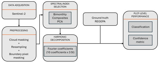
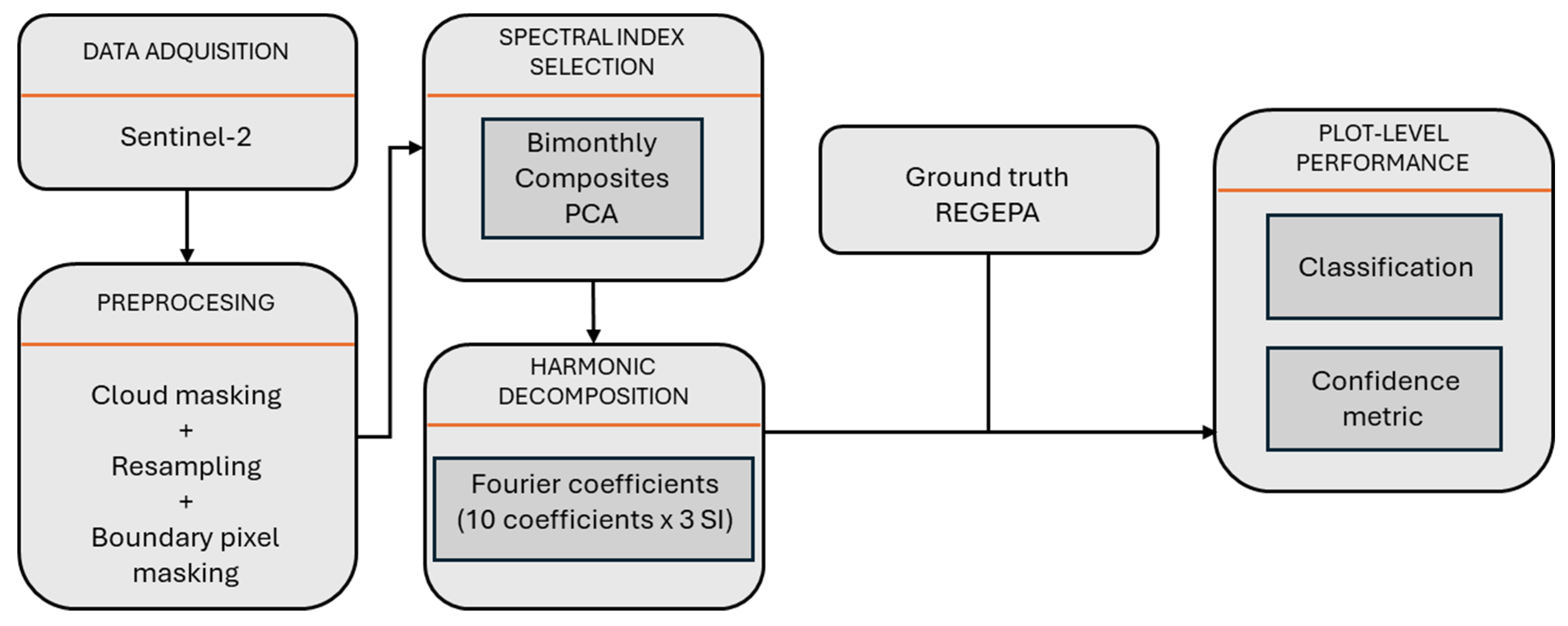
Figure 1 shows the workflow of the methodological approach carried out in the study.

Figure 1. Flowchart of the overall methodology.

2.1. Study Area

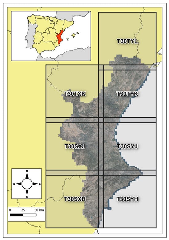
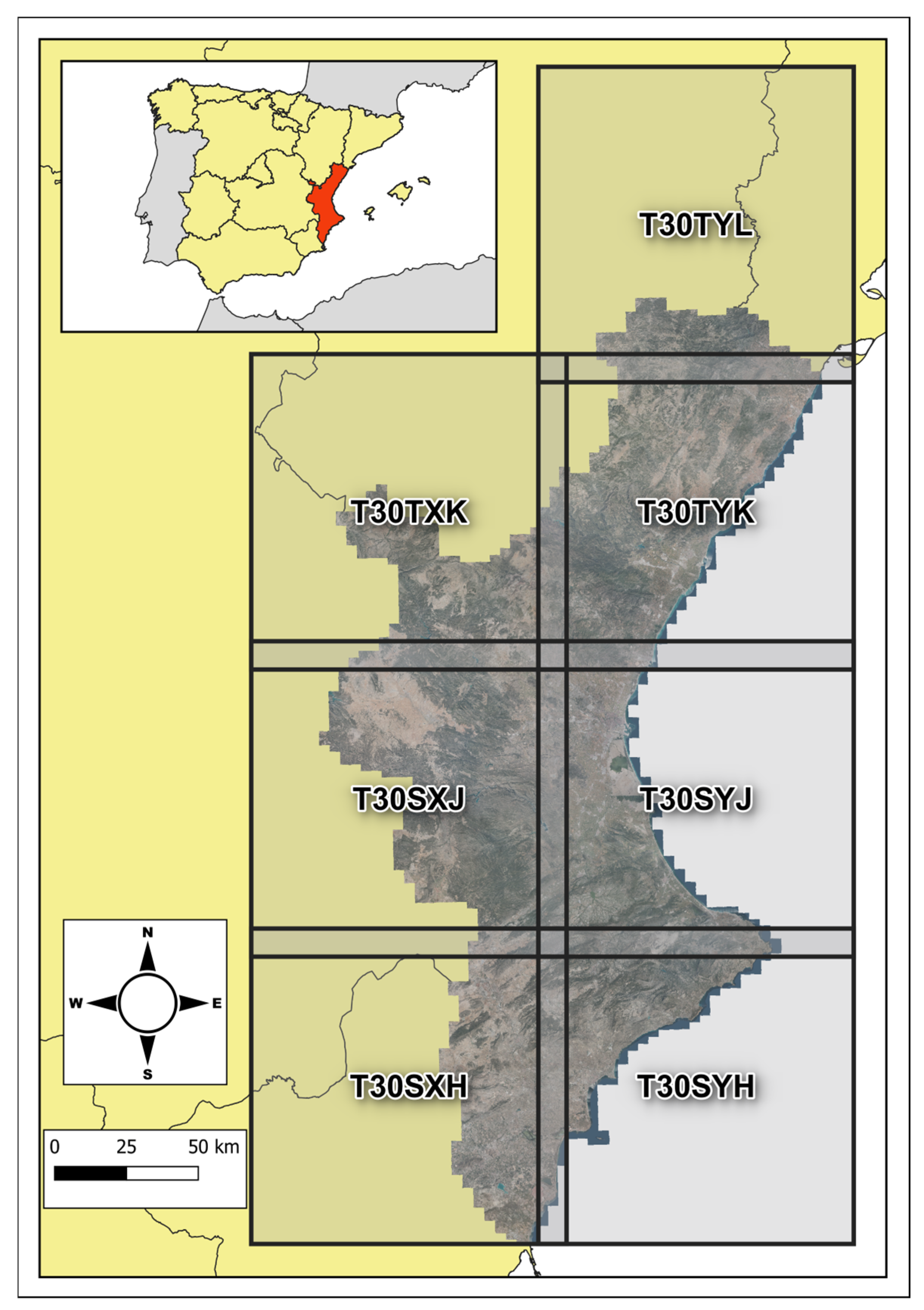
The study area selected was the entire CV, located in the east of Spain. The overlapping S2 tiles include 30TYL, 30TXK, 30TYK, 30SXJ, 30SYJ, 30SXH, and 30SYH (Figure 2). Covering an area of approximately 23,250 km², agricultural land comprises 37.4% of the region [33]. This area represents a typical Mediterranean agricultural landscape, with the dominant crops being citrus, almond, olive, vine and persimmon orchards, and rice fields. The average size of plots under study was 0.89 ± 1.10 ha (mean ± standard deviation).

Figure 2. Location of the study area and the overlapping Sentinel-2 tiles.

2.2. Ground Truth and Data Preprocessing

Ground-truth labels were obtained in 2023 from the Registro de Explotaciones Agrícolas de la Comunitat Valenciana (REA-CV), the regional geospatial register that integrates with Spain’s national agricultural registry (SIEX, Sistema de Información de Explotaciones Agrícolas y Ganaderas y de la Producción Agraria) and is maintained by the Valencian regional government [34,35]. The spatial boundaries of plots correspond to the official SIGPAC (Sistema de Información Geográfica de Parcelas Agrícolas) [36], while REA-CV provides the associated agronomic and descriptive attributes. The registry is updated annually via farmer declarations aligned with the Common Agricultural Policy and is subject to administrative checks and on-site inspections, which support the reliability of these labels.

Plots smaller than 0.3 ha [37] and those planted with less represented species (fewer than 10,000 plots in the study area) were removed from the study. Each remaining plot was assigned to one of 6 predefined classes (citrus (CI), almond (AL), olive (OL), vineyard (VI), persimmon (PE), and rice (RI)) based on the planted species in REA-CV. Each class encompassed all varieties of the selected species, with the citrus class including all mandarin and orange varieties. It is important to highlight that these classes include both permanent and seasonal crops, as well as evergreen and deciduous species. Among the permanent crops, trees in CI and OL classes are evergreen, while AL, VI, and PE are deciduous. RI corresponds to a seasonal, herbaceous crop.

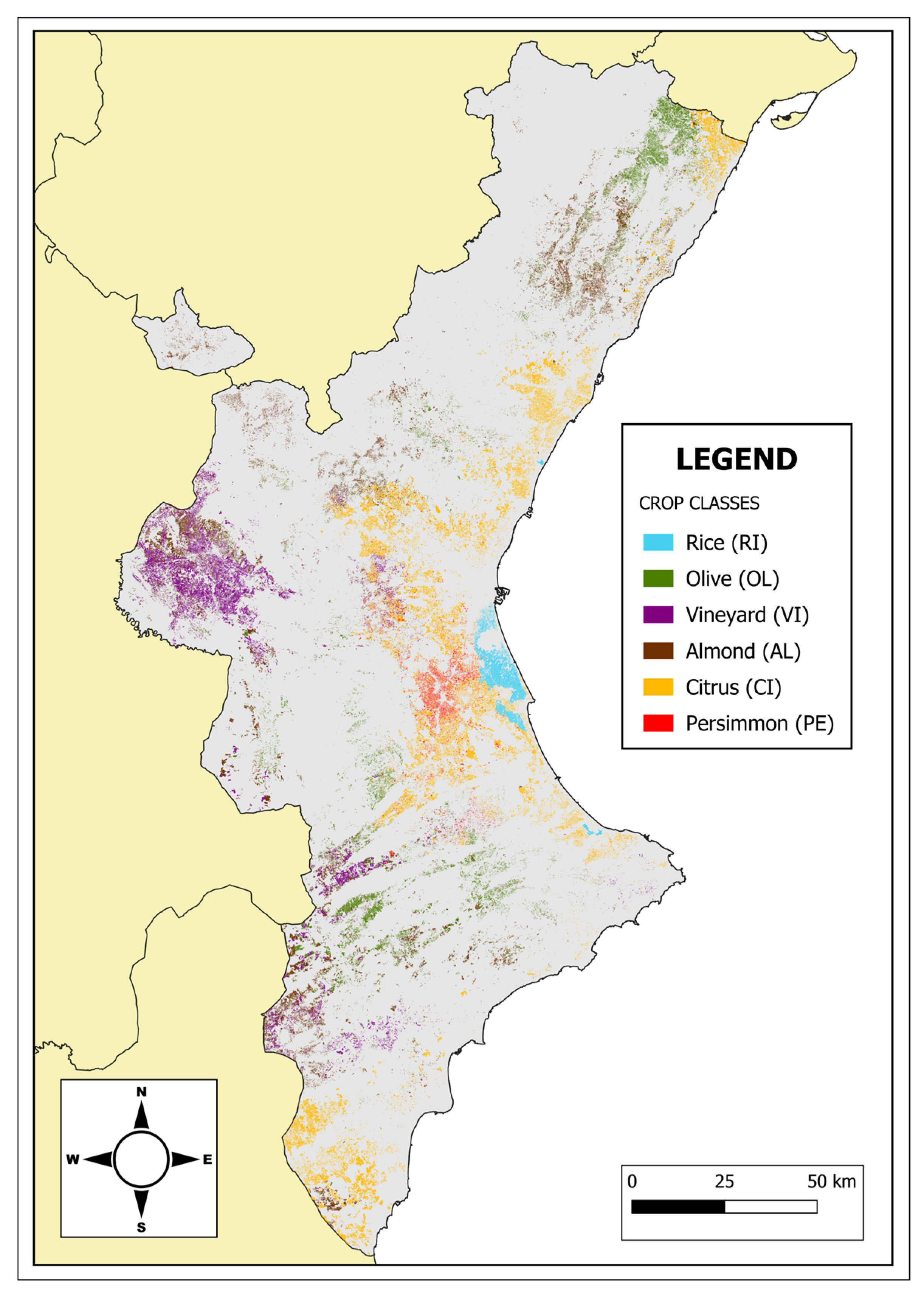
At the end of this process, a georeferenced database with 274,482 labeled plots was obtained. Figure 3 illustrates the REA-CV plots included in the study area, and Table 1 provides a summary of the number and size distribution of individual fields in each class.

Figure 3. Ground-truth data distribution over the study area after preprocessing.

Table 1. Summary of ground-truth data. Plot size is reported as mean ± standard deviation.

Class	Number of Plots	Plot Size (ha)
Rice (RI)	11,178	1.04 ± 1.14
Olive (OL)	53,569	0.79 ± 0.96
Vineyard (VI)	37,155	1.09 ± 1.25
Almond (AL)	54,217	0.99 ± 1.51
Citrus (CI)	103,939	0.85 ± 0.87
Persimmon (PE)	14,424	0.62 ± 0.52

Satellite data access and all subsequent preprocessing computations were conducted using the Google Earth Engine (GEE) cloud-computing platform (https://earthengine.google.com) [38]. Using the harmonized Sentinel-2 surface reflectance (Level 2A) product (COPERNICUS/S2_SR_HARMONIZED), a time-filtered image collection was generated to represent a single agricultural year (1 September 2022 to 31 August 2023). Only images with less than 30% cloudy pixels were included. Given that the study area overlaps seven S2 tiles, separate collections were created for each tile, resulting in a total of 517 images.

Cloud and cloud-shadow pixels were masked in all images using a conservative approach, as the study area generally experiences clear skies with minimal cloud cover throughout the year. Masks combined the cloud, cloud shadow, and thin cirrus classes from the Scene Classification (SCL) band of the L2A processing level with pixels having a cloud probability above 30% from the S2 Cloud Probability product (COPERNICUS/S2_CLOUD_PROBABILITY). All 20 m bands were finally resampled to 10 m resolution using bilinear interpolation.

High landscape fragmentation poses a major challenge for crop identification because plot boundary pixels provide very noisy information (e.g., fences, roads, or overlapping adjacent crops) and represent a relatively high proportion of the plot. For this reason, pixels not entirely contained within the plot’s defining polygon were masked, mitigating the limitations of Sentinel-2′s spatial resolution. This approach is particularly relevant in highly fragmented landscapes such as ours, where approximately 40% of pixels are located at plot edges. By excluding these pixels from the analysis, we ensure that the classification relies on pixels representing exclusively the crop. It is worth noting that this exclusion even implies that 601 plots were removed from the analysis due to their small size or because they had an elongated and narrow shape. Data in Table 1 do not include these plots.

2.3. Spectral Index Selection

Eleven spectral indices (Table 2) were selected to make explicit a set of design criteria aligned with our study goals: (i) to cover complementary biophysical domains relevant to the target classes: greenness/structure (NDVI, EVI, NDRE), soil-adjusted greenness for partial canopy cover (SAVI, OSAVI, OSAVIrd), canopy water status (NDMI, NDMI2, MSI, MSI2), and senescence (PSRI); (ii) to ensure Sentinel-2 readiness, deriving every index directly from MSI bands without ancillary parameters; (iii) to preserve interpretability in agronomic and phenological terms; (iv) to maintain operational simplicity, favoring closed-form indices with robust behavior across seasons; and (v) to maximize spectral coverage while limiting redundancy, which we subsequently examined using PCA. This criteria-driven selection provided a compact, yet complementary panel of indices for downstream modeling.

Table 2. SIs calculated on the reference dataset. For S2 Multispectral Instrument, $\rho$ Blue is band 2, $\rho$Red is band 4, $\rho$Rededge is band 6, $\rho$NIR is band 8, $\rho$SWIR1 is band 11, and $\rho$SWIR2 is band 12.

Spectral Index	Acronym	Formula	Reference
Normalized Difference Vegetation Index	NDVI	${\displaystyle \frac{{\rho }_{NIR}-{\rho }_{Red}}{{\rho }_{NIR}+{\rho }_{Red}}}$	[39]
Normalized Difference Red Edge Index	NDRE	${\displaystyle \frac{{\rho }_{NIR}-{\rho }_{Rededge}}{{\rho }_{NIR}+{\rho }_{Rededge}}}$	Adapted from [40]
Enhanced Vegetation Index	EVI	$2.5{\displaystyle \frac{{\rho }_{NIR}-{\rho }_{Red}}{\left({\rho }_{NIR}+6{\rho }_{Red}-7.5{\rho }_{Blue}\right)+1}}$	[41]
Soil Adjusted Vegetation Index	SAVI	${\displaystyle \frac{{\rho }_{NIR}-{\rho }_{Red}}{{\rho }_{NIR}+{\rho }_{Red}+0.5}}(1+0.5)$	[42]
Optimized Soil-Adjusted Vegetation Index	OSAVI	${\displaystyle \frac{{\rho }_{NIR}-{\rho }_{Red}}{{\rho }_{NIR}+{\rho }_{Red}+0.5}}(1+0.5)$	[43]
Optimized Soil-Adjusted Vegetation Index (Red edge)	OSAVIrd	${\displaystyle \frac{{\rho }_{NIR}-{\rho }_{Rededge}}{{\rho }_{NIR}+{\rho }_{Rededge}+0.16}}(1+0.16)$
Normalized Difference Moisture Index	NDMI	${\displaystyle \frac{{\rho }_{NIR}-{\rho }_{SWIR1}}{{\rho }_{NIR}+{\rho }_{SWIR1}}}$	Adapted from [44] *
Normalized Difference Moisture Index-2	NDMI2	${\displaystyle \frac{{\rho }_{NIR}-{\rho }_{SWIR2}}{{\rho }_{NIR}+{\rho }_{SWIR2}}}$
Moisture Stress Index	MSI	${\displaystyle \frac{{\rho }_{SWIR1}}{{\rho }_{NIR}}}$	[45]
Moisture Stress Index-2	MSI2	${\displaystyle \frac{{\rho }_{SWIR2}}{{\rho }_{NIR}}}$
Plant Senescence Reflectance Index	PSRI	${\displaystyle \frac{{\rho }_{Red}-{\rho }_{Blue}}{{\rho }_{Rededge}}}$	[46]

* The authors referred to this index as NDWI in the original paper.

It is well known that SIs in agricultural scenes are often highly correlated, leading to redundant information. Principal component analysis (PCA) [47,48] was applied to assess SI correlation structure and identify those SIs that provided complementary, less correlated information. Six bimonthly image composites (September–October, November–December, January–February, March–April, May–June and July–August) were created for each tile image collection to examine whether these correlation structures varied over time. Bimonthly images from the same period of each tile were merged into a single image representing the entire study area. Subsequently, the principal components (PCs) of the eleven-dimensional space were computed for each image. PCs are new orthogonal (uncorrelated) variables that are linear combinations of the original ones, ordered by explained variance.

Biplots were used to visually represent the correlations among SIs and their contributions to the PCs. In these plots, SIs appear as vectors from the origin. Their direction and length indicate the correlation and strength of each SI’s contribution to the PCs. Thus, vectors close to each other indicate correlated, redundant information, while near-orthogonal vectors indicate uncorrelated, complementary information. Biplots displaying the first three PCs were analyzed, from which three SIs (NDMI, NDRE, and PSRI) were selected for their minimal redundancy and high relevance.

While random forests are typically robust to multicollinearity in terms of predictive performance, strong correlations among spectral indices can make importance estimates unstable and hinder attribution. To prioritize interpretability, we applied this a priori, correlation-informed selection based on PCA biplots computed on six bimonthly composites per tile. By examining the geometry of SI vectors in the first three principal components across periods, we retained indices that contributed complementary, near-orthogonal information. It is important to remark that PCA was used only as an exploratory tool: the classifier was trained on the original indices rather than on transformed components. This procedure reduced redundancy and computational load while preserving a compact, agronomically and phenologically interpretable feature set, ensuring the classifier received complementary information (see Section 3.1 for examples).

These analyses were conducted using R v4.2.2 [49]. PCA was performed with the default “stats” package, biplots were generated with “factoextra” v1.0.7 [50], and data wrangling was performed using “dplyr” v1.1.4 [51].

2.4. Fourier Approximation of Time Series

As described in Section 2.2, each image collection is a temporal sequence of images within its respective tile. The three selected SIs (NDMI, NDRE, and PSRI) were calculated on each image of the collections. As a result, three image arrays were generated, one per SI, namely image arrays 1, 2, and 3 (IA1, IA2, IA3). In such images, each pixel was a 1×N array, where N is the number of images in the collection, thus representing the variation of the SI over time of each pixel.

Time series can be decomposed in harmonic terms using Fourier analysis to identify dominant periodic (seasonal) patterns of data [18,19]. Each harmonic term captures a specific frequency pattern within the series. The first harmonic can be associated with cycles with a unimodal pattern, i.e., a unique SI peak over one agricultural year. The second harmonic is related to phenological cycles with a bimodal pattern, and higher-order terms reflect higher periodicities.

Complex time series can be reconstructed with a limited number of harmonic terms, because each term accounts for a portion of the total variance of the original series. For instance, in annual crops with unimodal seasonal behavior, approximately 95% of the variance can be explained by the first four harmonics and around 90% in crops with bimodal patterns [19]. In this work, we used the first four harmonics to reconstruct spectral-index time series, aiming to capture dominant seasonal phenology while attenuating high-frequency noise. The 1st–2nd harmonics represent annual and semiannual components, and the 3rd–4th harmonics summarize sub-seasonal dynamics without reproducing short-term fluctuations. This choice follows the common observation that the first 3–5 harmonics explain most of the variance in vegetation time series [19]. In preliminary exploration, reconstructions with three harmonics appeared oversmoothed, whereas five harmonics tended to track short-lived perturbations. Four harmonics provided the most faithful seasonal trajectory. For consistency and interpretability, the order was fixed a priori for all indices and tiles, yielding a compact, phenology-aware descriptor for downstream classification.

The Fourier approximation of the temporal series in our study was expressed by Equation (1):

$$f\left(x\right)=c_0+c_{1}x+\sum _{n=1}^4{a}_n\cos \left(2\pi nx\right)+b_n\sin \left(2\pi nx\right)$$

(1)

where n represents the frequency of the harmonic term, and $c_0$, $c_1$, $a_n$, and $b_n$ are the harmonic coefficients. $c_0$ and $c_1$ are the coefficients for the constant and linear terms that define the baseline and trend, and $a_n$ and $b_n$, are the coefficients for the cosine and sine terms, which determine the amplitude and phase of the sinusoidal waves. These coefficients were calculated at the pixel level by fitting the time series of each pixel of IA1, IA2, and AI3 to $f\left(x\right)$ using ordinary least squares regression. Consequently, three new image arrays were created, each pixel composed of a 1 × 10 array and each array component being the values of the 10 harmonic coefficients. Array images were flattened and then joined to form a single image composed of 30 bands (10 coefficients per 3 SI). This process was applied to the 7 image collections, and the final images of the collections were merged to form a single image of the entire study area. The ground-truth class was added as a new band, assigning the corresponding class value to all the pixels inside each plot. The Fourier decomposition of the time series was conducted using GEE.

2.5. Classifier

Among the different supervised classification algorithms available, random forest (RF) was selected. This is an ensemble learning method that combines multiple decision trees to make more accurate predictions. RF creates a collection of decision trees where every decision tree is trained independently with a random subset of the complete training data and its nodes are split considering a random subset of the variables incorporated into the classifier. Such randomness helps reduce overfitting and enhances the model’s generalization ability. For classification tasks, the final assignation is given by the most frequent class obtained from all decision trees in the ensemble.

The training–testing procedure was carried out using Spyder v5 [52], an integrated development environment (IDE) written in and for Python [53]. The Python version used was 3.12.5.

RF was implemented using the “scikit-learn” module [54]. The number of features per split was set to the square root of the total number of features. The minimum number of samples required to be at a leaf node was set to 1. The maximum depth of the tree was not set, so the number of nodes per tree was not limited. Out-of-bag (OOB) samples were allowed to be used to estimate the generalization score. The optimal number of trees was estimated by building a pixel-level classifier with 80% of the training samples and plotting the overall accuracy and the OOB error over the remaining 20% of samples (validation subset). The classifier was run with an increasing number of trees: 1, 5, and 10 from 20 to 100 in steps of 20, and from 200 to 500 in steps of 100. Considering the outcome (Section 3.3), 200 trees were considered optimal.

To address class imbalance (Table 1), an equal number of training plots was selected for each class, preventing bias toward the majority class (citrus). The number of training plots was set to 7000 per class, ensuring that the minority class (RI) retained at least 40% of its plots for testing. Consequently, 42,000 plots were used for training, with the remaining 232,482 plots reserved for testing.

Feature importance indicates how much each input feature influences the model’s predictions. In this study, the importance of the input features (SI Fourier coefficients) was assessed using a permutation strategy, where each feature’s contribution was evaluated by comparing the model’s accuracy with and without that feature. Specifically, the values of each feature were randomly permuted, meaning that the original order of the feature’s values was scrambled, thereby disrupting the relationship between that feature and the target variable, while the values of the other features remained unchanged. The model was then reevaluated for each permutation. To ensure reliable results, this process was repeated 10 times for each feature, providing a consistent measure of its impact on model performance.

2.6. Confidence Metrics at Pixel and Plot Level

The probability of a pixel belonging to each one of the classes was estimated by counting the relative numbers of trees voting for each class. Then, the pixel was initially assigned the class having the highest probability. However, in a second step, all pixels whose maximum probability was lower than twice the second-highest probability were masked, and thus pixels with less confidence in class assignment were removed from subsequent calculations. Consequently, some of the study plots were removed after this process, since there were no pixels left in them that fulfilled the rule.

Each plot was assigned a class by computing the mode of the unmasked pixels inside its perimeter. In a subsequent step, a confidence metric at a plot level ($C_o$) was calculated following Equation (2):

$$C_o=100 \mu w$$

(2)

$$\mu =M/T$$

(3)

$$w=f\left(r\right)=f(T/I)$$

(4)

where µ is the ratio of the number of mode-class unmasked pixels (M) versus the total number of unmasked pixels inside the plot (T) (Equation (3)), and w is a weighting factor ranging from 0 to 1, related to the ratio of (T) versus the initial number of pixels inside the plot before masking (I) (Equation (4)). w weights were arbitrarily defined in 0.1 steps (Table 3). For instance, for a plot with r ∈ [0.1, 0.2[, the confidence level of the plot was reduced by half (w = 0.5). Furthermore, when r > 0.5, the confidence level of the plot was not reduced (w = 1).

Table 3. w values as a function of r.

r Values	w Value
r < 0.1	0
0.1 ≤ r < 0.2	0.5
0.2 ≤ r < 0.3	0.6
0.3 ≤ r < 0.4	0.7
0.4 ≤ r < 0.5	0.8
r > 0.5	1

2.7. Performance Assessment

The accuracy of the classifier was assessed by computing the confusion matrix and several standard measures derived from it [55], such as the overall accuracy (OA), the producer’s and the user’s accuracy (PA and UA respectively), and the kappa index (k) [56].

With an established confidence metric for plot-level class assignment, we examined how increasing the confidence threshold impacted classification accuracy. Naturally, raising this threshold reduces the number of plots eligible for classification. Section 3.5 illustrates this trade-off, showing overall classifier accuracy at various confidence levels and the corresponding percentage of plots remaining eligible for classification.

3. Results

3.1. Spectral Index Selection

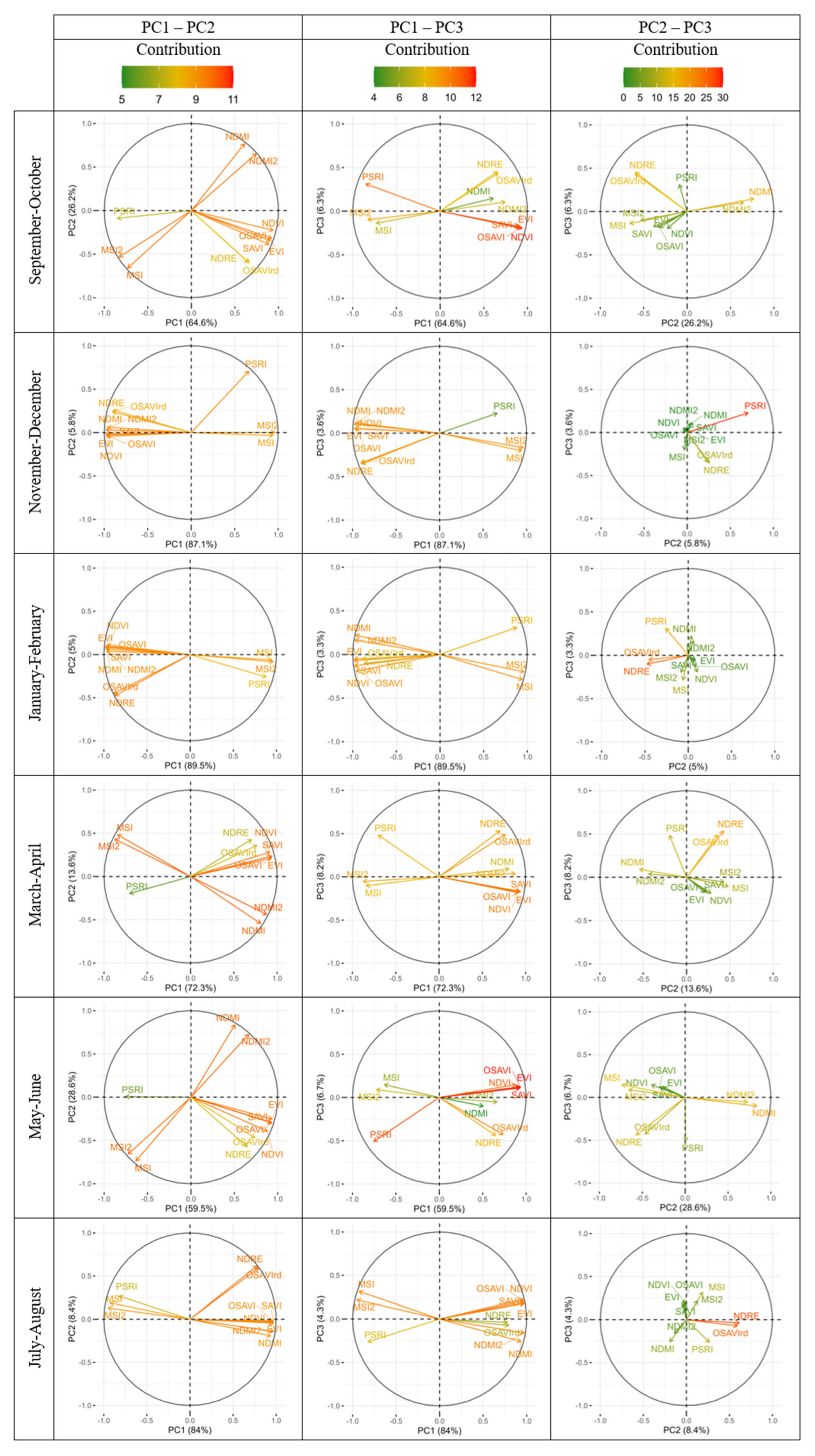
This section presents the results of the vegetation index selection using PCA, as described in Section 2.3. Figure 4 displays biplots for each two-month period, plotting SI against pairs of the first three principal components (PCs). These PCs capture a substantial portion of the variance within each period. For example, in September–October, they explain 97.1% of the variance, with PC1, PC2, and PC3 accounting for 64.6%, 26.2%, and 6.3% of the variance, respectively.

Figure 4. Bimonthly biplots of first 3 PCs of all SIs defined in Table 2.

Biplots of PC1 and PC2 (left column) illustrate slight variations in the correlation structures of SIs over time, though some consistent patterns are evident. The vegetation indices, termed Group A, can be further divided into Group A.1 (NDVI, EVI, SAVI, OSAVI) and Group A.2 (OSAVI_RD and NDRE). Both subgroups are closely associated and highly correlated with PC1, yet Group A.2 shifts away from Group A.1, contributing more to PC2 during certain periods, such as January–February and July–August. Notably, Group A.2 indices incorporate red-edge band information.

The moisture indices, termed Group B, can be divided into Group B.1 (NDMI and NDMI2) and Group B.2 (MSI, MSI2), which are approximately 180° apart, indicating a strong negative correlation. In some bimonthly periods, like September–October, March–April, and May–June, Group B correlates with PC2. However, in November–December, January–February, and July–August, Group B.2 shifts closer to Group A.1, contributing more to PC1, a trend that aligns with a decrease in Group A.2′s contribution to PC1 during these months.

PSRI, a commonly used senescence index, is expected to show a negative correlation with Group A indices. This pattern is observable in January–February and July–August, when PSRI is positioned near Group B.2. However, in other periods, PSRI behaves somewhat differently, correlating with PC1 across most periods except November–December, when it aligns more closely with PC2. The contribution of each SI to the variance explained by PC1 and PC2 ranges from 5% to 11%.

Biplots of PC1 and PC3 (central column) show fewer temporal variations in SI correlation structures. In these plots, groups A.1 and B.1 are positioned closer together, while Group B.2 lies approximately 180° opposite B.1, all correlated with PC1. Both PSRI and Group A.2, though close to Groups B.2 and A.1, respectively, exhibit slightly stronger correlations with PC3 than other indices. SI contributions to the variance explained by PC1 and PC3 remain in the range from 4% to 12%.

Biplots of PC2 and PC3 (right column) reveal that indices in Group A.1 contribute minimally to the joint variance explained by these components. Group A.2 shows a notable contribution, mostly correlating with PC2. Group B.1 also aligns with PC2 in periods like September–October and May–June. PSRI is generally correlated with PC3, except during the November–December period. Contributions of SIs to the variance explained by PC2 and PC3 have a wider range, from 0% to 30%.

These biplots indicate strong correlations among SIs within the same groups. Therefore, three SIs were chosen for subsequent calculations, each representing a different group, to streamline our classification models by using a few uncorrelated variables. From Group A, we selected NDRE (A.2), which captures variations in correlation structures over time. From Group B, we selected NDMI (B.1) due to its stronger correlation with PC2 during certain bimonthly periods. PSRI was also selected for its distinct behavior relative to other indices. These SIs act as proxies for key vegetation parameters: moisture (NDMI), vigor (NDRE), and senescence (PSRI). Examples of biplots that effectively display the orthogonality and thus the uncorrelated information of these three indices include the PC1–PC2 biplots for September–October, March–April, and May–June.

3.2. Fourier Approximation of Time Series

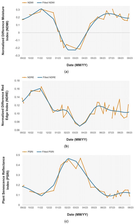
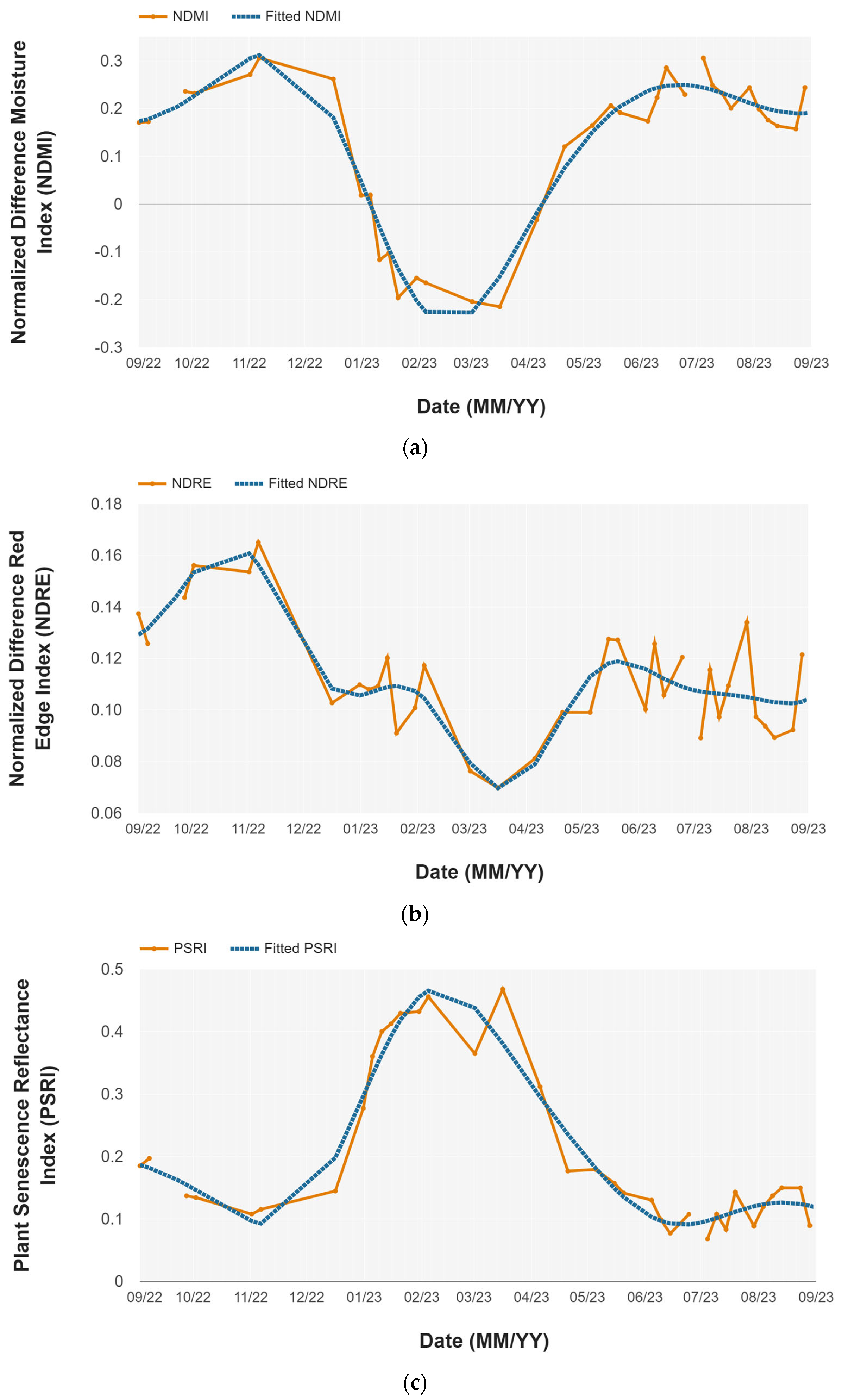
Figure 5 illustrates the temporal evolution of NDMI, NDRE, and PSRI for a randomly selected pixel in the persimmon class (PE). The Fourier decomposition provides a good approximation of the observed values. Table 4 shows that all classes were well fitted, with average root mean square errors (RMSE) at the pixel level of approximately 0.02, 0.01, and 0.02 for NDMI, NDRE, and PSRI, respectively, except for the rice class (RI), where RMSE values were higher (0.11, 0.03, and 0.09, respectively). It is worth noting that although the RMSE for NDMI and PSRI was higher, these indices also exhibited a larger range of variation.

Figure 5. Example of time-series fitting for a sample pixel in the PE class using Fourier decomposition (a) NDMI, (b) NDRE, and (c) PSRI. Observed values (orange continuous line) and fitted (blue dashed line).

Table 4. RMSE (mean ± 2 standard errors) between the fitted Fourier series and the observed time series for each index depending on the class.

Class	NDMI	NDRE	PSRI
Rice (RI)	0.10932 ± 0.00048	0.03139 ± 0.00035	0.08650 ± 0.00215
Olive (OL)	0.02196 ± 0.00006	0.01663 ± 0.00004	0.02718 ± 0.00005
Vineyard (VI)	0.02225 ± 0.00006	0.01432 ± 0.00003	0.02936 ± 0.00008
Almond (AL)	0.02460 ± 0.00007	0.01576 ± 0.00004	0.03074 ± 0.00007
Citrus (CI)	0.02459 ± 0.00004	0.01396 ± 0.00002	0.02361 ± 0.00003
Persimmon (PE)	0.03048 ± 0.00015	0.01419 ± 0.00005	0.02862 ± 0.00009

For evaluation of the Fourier fits, RMSE was computed between the fitted harmonic function and the observed SI time series after cloud/shadow masking (Section 2.2), using only valid observations at their original time stamps. Because the reconstruction is restricted to the first four harmonics, it retains the dominant seasonal component while suppressing non-periodic, high-frequency variability. Within this setup, RMSE serves as a meaningful measure of phenological signal extraction quality, indicating how closely the truncated harmonic model tracks the seasonal dynamics.

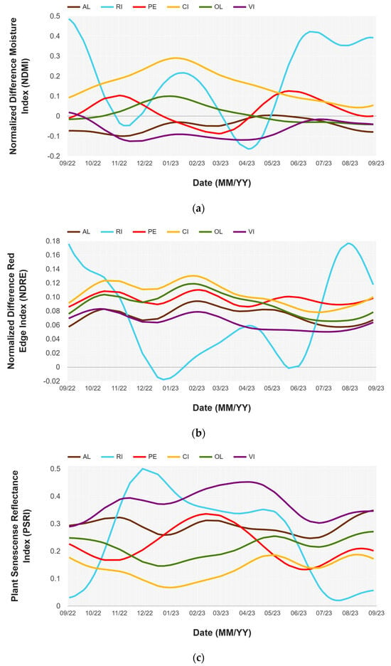
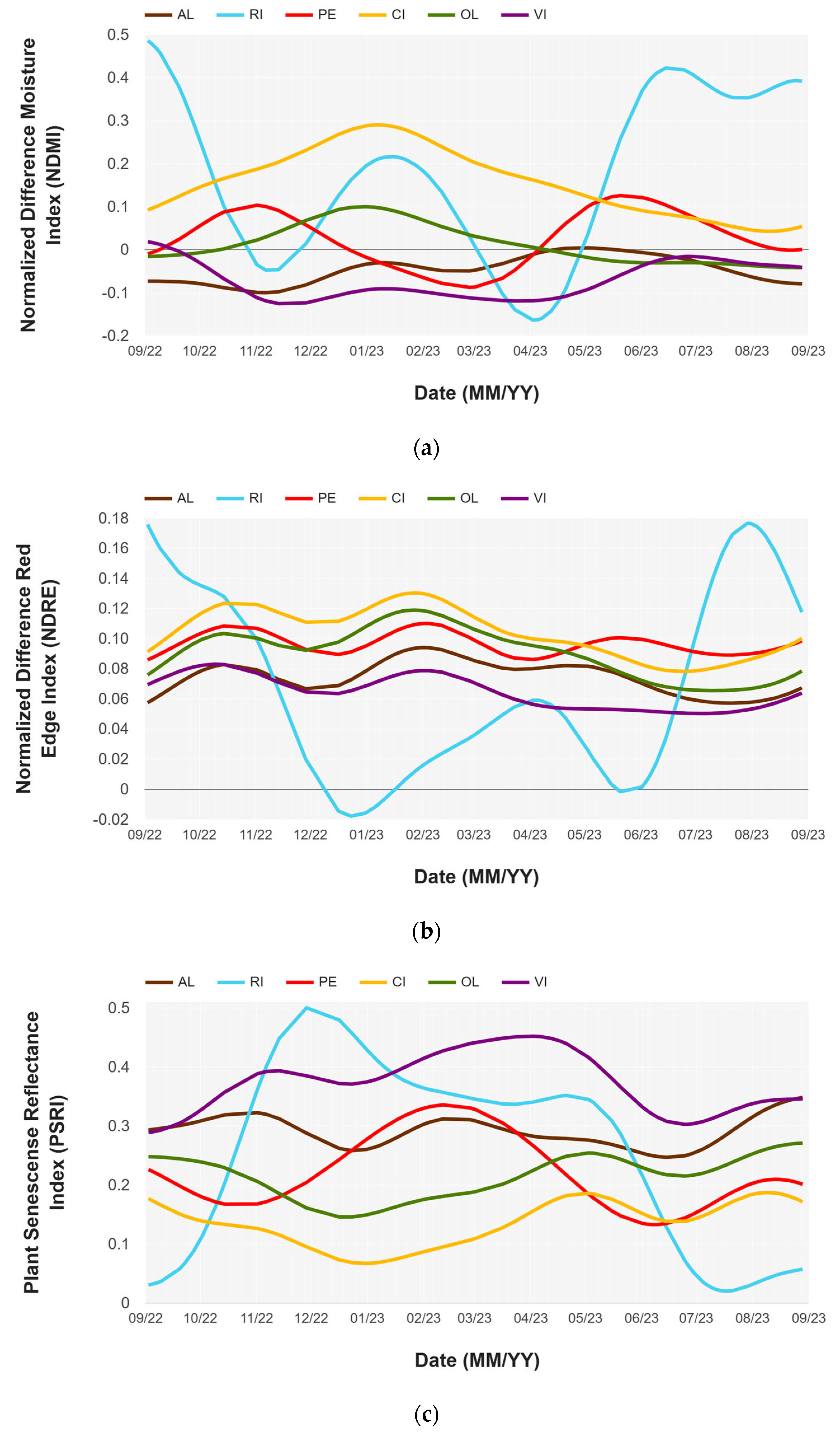
Graphs like those in Figure 6 can be created by averaging the harmonic-derived time series of each SI across the studied classes. Overall, the fitted time series exhibit distinct patterns depending on the class, indicating specific time windows where major differences emerge.

Figure 6. Average harmonic-derived time series of (a) NDMI, (b) NDRE, and (c) PSRI for each class. Only plots within the 30SYJ tile were considered.

The most distinct pattern is seen in the RI class, which differs notably from other classes across all three indices. This difference is primarily due to rice being the only annual, non-woody crop in the study. Its unique phenology and management practices set it apart. NDMI values remain high from May through early September, corresponding to the period when fields are flooded. NDRE peaks at the end of September, just before harvest, while PSRI reaches its highest values between November and February, as the straw residue left after harvest decomposes in the fields.

The remaining crop classes exhibit similar seasonal patterns, though some distinctions are more apparent in the NDMI evolution (Figure 6a). CI and OL classes display a unimodal pattern, with a peak from late autumn to winter (November to March), followed by reduced values in the summer. CI shows higher NDMI values and a broader range of variation throughout the year. The AL and VI classes have similar patterns with minimal seasonal variation, both exhibiting the lowest NDMI values among all classes, although almond-class values are slightly elevated in winter and spring. The PE class, however, follows a bimodal pattern, peaking in November and again in May, with a distinct low point in March.

Figure 6b illustrates NDRE variation across crop classes, showing consistent patterns among woody classes with minimal seasonal variation. This steady behavior aligns with expectations for the evergreen CI and OL classes, but is more surprising for deciduous tree classes like AL, PE, and VI, where greater differentiation between leafy and leafless seasons might be anticipated. Among woody classes, CI and OL display the highest NDRE values, followed by PE, while AL and VI exhibit the lowest values.

The PSRI variation patterns shown in Figure 6c appear to be inversely related to those of NDRE (Figure 6b), but with greater separability among classes. Here, the VI and AL classes have the highest PSRI values, while OL and CI classes have the lowest. The PE class, displaying a bimodal pattern like NDMI (Figure 6a), reaches its highest PSRI value in March.

Overall, CI and OL classes consistently present the highest NDMI and NDRE values and the lowest PSRI values throughout the year, reflecting their evergreen nature. Although both classes show similar trends, the CI class often registers higher values, likely due to its denser canopy. Among the deciduous tree classes, AL and VI stand out with the lowest NDMI and NDRE values and the highest PSRI values, with VI values being particularly distinct. PE-class patterns fall between these extremes, while the RI class exhibits unique patterns entirely distinct from the other classes.

3.3. Optimal Number of Trees and Feature Importance

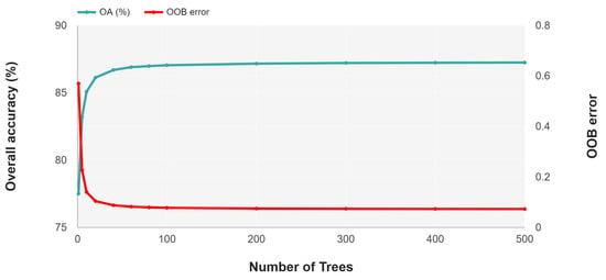
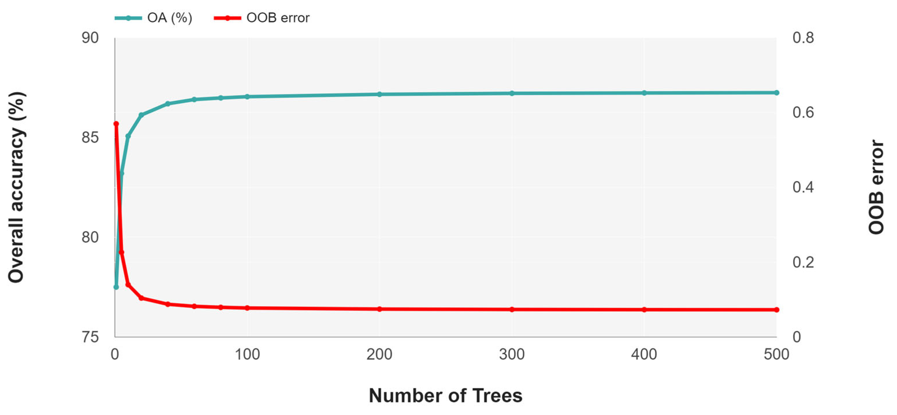
Figure 7 displays the overall accuracy (OA) achieved by the classifier on the validation subset, alongside the out-of-bag (OOB) error, as the number of trees in the random forest model increases. As shown, both the OA and the OOB error stabilize after reaching 100–200 trees, indicating that further increases in the number of trees beyond 200 are unlikely to result in significant changes in these performance metrics.

Figure 7. Influence of the number of decision trees on the OA and the OOB error achieved by the classifier.

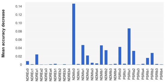
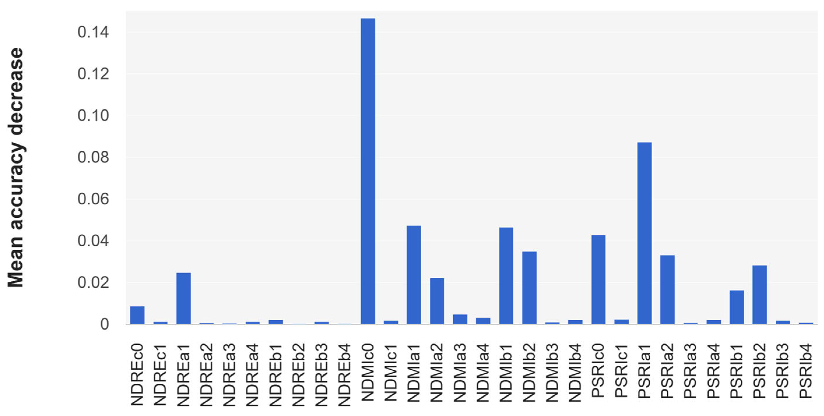
Figure 8 illustrates the importance of each input feature, showing the mean accuracy decrease when a particular feature is excluded from the model. For each of the three selected indices (NDMI, NDRE, and PSRI), each input feature represents one of the calculated Fourier coefficients by fitting the time series of each index to Equation (1) (Section 2.4). Letters after the index name refer to the coefficients c₀, c₁, a_i, and b_i.

Figure 8. Importance of the input features (SI Fourier coefficients). Letters after the index name refer to the coefficients c₀, c₁, a_i, and b_i in Equation (1).

The most important predictors are those derived from the NDMI and PSRI. The input feature whose permutation generates the greatest decrease in accuracy is NDMIc0 (c₀ for the NDMI), the baseline value for the time series over which the harmonics oscillate. Other important predictors are the features related to the first two harmonics (NDMIa1, NDMIa2, NDMIb1 and NDMIb2). This aligns with Figure 6a, where the variations observed in the classes throughout the time series refer mainly to unimodal and bimodal patterns. For the PSRI, the most important coefficients are the same as for the NDMI, although with slightly less importance.

In contrast, NDRE seems to offer less relevant information, as permuted features derived from it do not significantly impact the classifier’s accuracy. This observation is consistent with the findings in Figure 6b, where, as previously noted, most of the woody classes show similar patterns for this index.

3.4. Classification Performance

As described in Section 2.6, all pixels with a maximum membership probability lower than twice the second-highest probability were masked. As a result, 0.45% of the plots under study (1052 plots) were excluded from classification at the plot level, as all pixels within these plots were masked.

Table 5 shows the confusion matrix and performance values at the plot level obtained by the classifier (OA = 86.85% and k = 0.82). It demonstrates that 99.95% of RI, 81.85% of OL, 93.53% of VI, 86.31% of AL, 86.59% of CI, and 90.19% of PE were correctly classified. Exclusion errors were around 10% for all classes, except for RI, where there was virtually no exclusion error, and for OL, where the exclusion error was close to 20%. AL contributed the most to this percentage of exclusion error (around 11% out of 20%). Similarly, OL contributed the most to the exclusion errors for AL (around 9% out of 14%). These two classes were also the primary contributors to the exclusion errors in CI (around 6% for OL and around 4% for AL, out of 13%).

Table 5. Confusion matrix and performance values (OA and kappa) of the classifier. Classes: rice (RI), olive (OL), vineyard (VI), almond (AL), citrus (CI), and persimmon (PE).

		Ground Truth						Total	UA (%)
		RI	OL	VI	AL	CI	PE
Classified	RI	4175	6	12	9	29	1	4232	98.65
	OL	0	37900	435	4036	5944	95	48410	78.29
	VI	1	611	28139	1624	1056	94	31525	89.26
	AL	0	5250	1223	40518	4227	236	51454	78.75
	CI	1	2288	100	285	83576	300	86550	96.56
	PE	0	247	175	475	1684	6678	9259	72.12
Total		4177	46302	30084	46947	96516	7404	OA = 86.85%
PA (%)		99.95	81.85	93.53	86.31	86.59	90.19	k = 0.82

There were more notable differences between classes in user accuracies (UAs). The highest UAs were achieved by RI and CI classes: 98.65% of the plots classified as rice were correctly identified, and the same applied to 96.56% of citrus orchards. The UAs for the OL and AL classes were 78.29% and 78.75%, respectively. Inclusion errors for AL were mainly due to confusion with the OL and CI classes (around 10% and 8% out of 21%, respectively). Inclusion errors for OL were primarily due to confusion with AL and CI (around 8% and 12% out of 22%, respectively). AL and CI also contributed significantly to the inclusion errors in the vineyard class (around 5% and 3% out of 11%, respectively). The lowest UA was 72.12%, achieved by PE, where around 18% of orchards classified as persimmons were actually planted with citrus.

This inter-class confusion can be largely attributed to the overlap of phenological patterns in the spectral indices analyzed (Figure 6), particularly NDMI and PSRI, from which the most important predictors were derived. For both indices, the time series of AL and OL exhibit substantial overlap from April to October, with maximum differences not exceeding 0.2 points for NDMI and 0.1 points for PSRI. Larger differences are observed between AL and CI, especially during winter, when AL, being a deciduous crop, has no leaves, whereas CI remains evergreen. However, from April onwards, once both crops present foliage, these differences diminish notably. OL and CI also show highly similar seasonal patterns in both indices. CI tends to have higher NDMI and lower PSRI values, presumably due to its denser canopy, but these differences may not be large enough to allow the classifier to fully separate them. Regarding PE, despite having distinct seasonal trajectories relative to CI, both classes substantially overlap from May to November, which likely explains why some CI plots are misassigned to the PE class.

It is also important to note that Figure 6 displays the average harmonic-derived time series from only one of the seven analyzed tiles, and variability among plots is expected. Not all plots within a given crop class necessarily follow the mean temporal pattern, and some individual plots may resemble the trajectories of other classes. These cases are the most likely contributors to the observed inclusion errors.

Overall, the separability among the AL, OL, and CI classes was lower than that between the other classes. As expected, RI exhibited the highest separability due to its distinct phenological cycle and its status as the only non-woody crop.

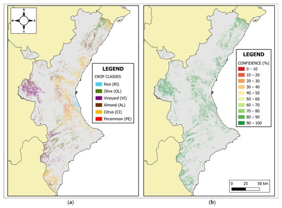
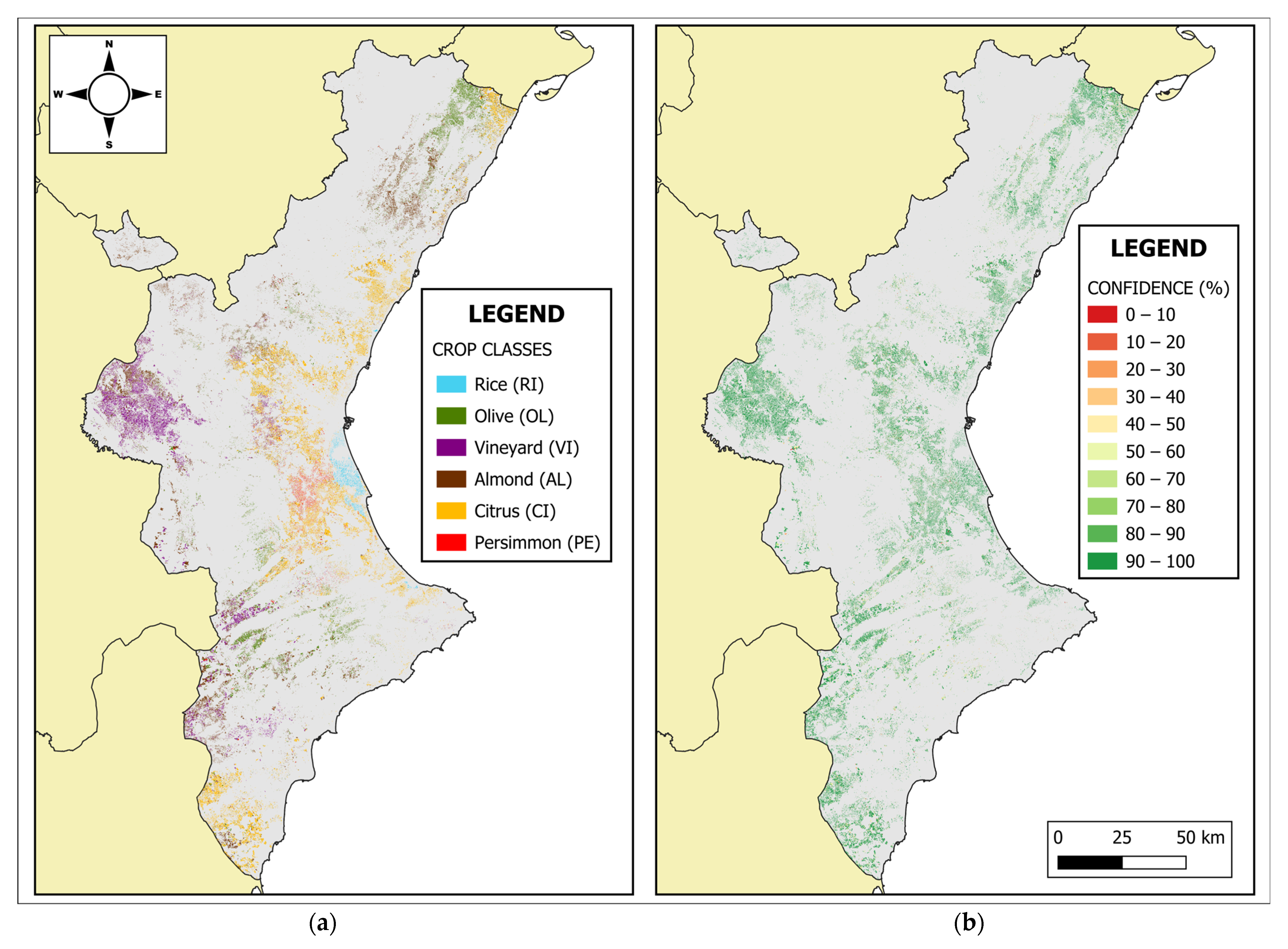
Figure 9 shows the classification map obtained for the testing set, along with the associated classification confidence map. Overall classification confidence is high, as indicated by the predominance of green values.

Figure 9. Classification map (a) and associated confidence level (b) for the testing set.

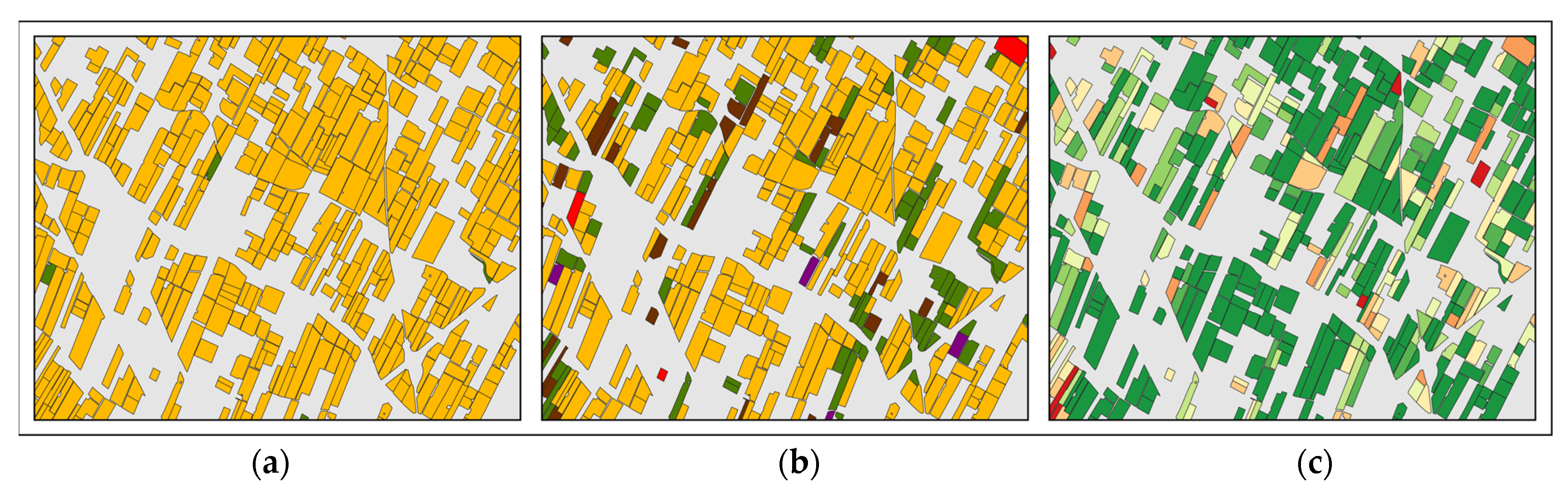
To visually highlight the exclusion errors associated with the citrus class, a citrus-growing area of approximately 7.5 km² in the far northeast of the CV is zoomed in for illustration. Figure 10 presents the ground truth (Figure 10a), the classification map (Figure 10b), and the confidence levels (Figure 10c) for this area. As previously explained, misclassifications involving the OL and AL classes were the primary sources of error (Figure 10b). The figure also demonstrates how misclassified orchards tend to have lower classification confidence values (Figure 10c), showcasing the usefulness of confidence levels in supporting decision-making.

Figure 10. (a) Ground truth, (b) classification result and (c) confidence level for a citrus-growing area in the northeast of CV. Colors in (a,b) correspond to those in the legend of Figure 9a. Colors in (c) correspond to those in the legend of Figure 9b.

3.5. Effect of the Confidence Level in Plot Classification

The confidence map provides an operational control to balance classification accuracy and the proportion of plots acted upon. By selecting a threshold, regional authorities can estimate effort (number of plots, staff, logistics), prioritize inspections (inspecting first plots where the classified crop disagrees with the declaration and confidence is high), and streamline screening (for low-confidence cases, photo interpretation is typically sufficient). Plots verified on-site can be incorporated into future training to improve model robustness, while plots left uninspected retain acceptable accuracy under the chosen threshold. This makes the metric directly useful for resource allocation and risk-based monitoring in real agricultural workflows.

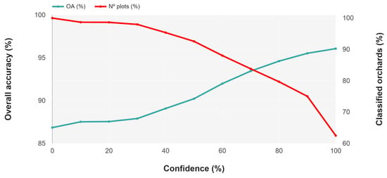
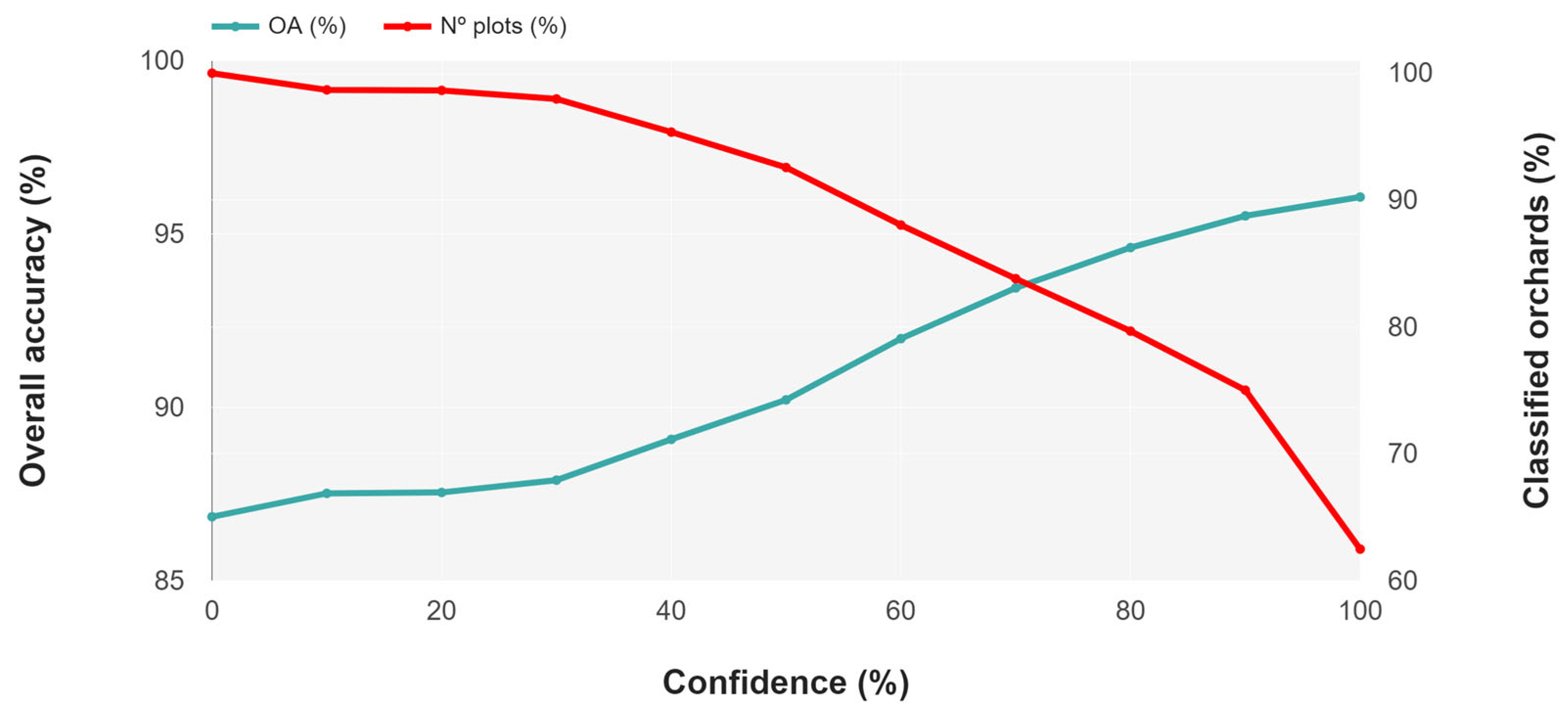
Figure 11 illustrates the relationship between overall accuracy (OA) and the confidence level applied to plot-class assignments, as defined in Section 2.6. As the confidence threshold increases, plots with a confidence level below the threshold are excluded from classification, which in turn reduces the percentage of plots classified.

Figure 11. OA and percentage of classified plots as a function of the confidence level.

At a 0% confidence level, all plots are eligible for classification, resulting in a mean OA of 86.85%. Conversely, when the confidence level is set to 100%, only 62.5% of the plots are classified, but the mean OA increases to 96.06%. Notably, both trends show accelerated changes once the confidence level exceeds 50%. However, the rate of decrease in the percentage of classified plots (from 100% to 62.5%) is more pronounced than the rate of increase in OA (from 86.85% to 96.06%).

This highlights a key trade-off in plot classification: while higher confidence levels yield higher OA, they also result in fewer plots being classified. Since unclassified plots would require additional effort for class assignment, such as expert decisions based on orthophotos or use of supplementary data, it is crucial to find an optimal balance between classification accuracy and the percentage of classified plots.

Table 6 demonstrates the application of the proposed classification scheme in a specific scenario with a 70% plot-classification confidence level. At this threshold, the overall accuracy (OA) increases from 86.85% to 93.44%, but 16.19% of plots become unclassified.

Table 6. Variation in classifier performance when setting a 70% threshold for plot-class confidence level compared to no threshold.

Class	Number of Plots (No Threshold/70%)	Plot Loss (%)	Producer’s Accuracy (No Threshold/70%)
RI	4177/4175	0.05	99.95/99.95
OL	46,302/35,064	24.27	81.85/88.33
VI	30,084/27,892	7.29	93.53/97.02
AL	46,947/37,986	19.09	86.31/93.22
CI	965,16/82,146	14.89	86.59/94.06
PE	7404/6696	9.56	90.19/94.97
Overall	231,430/193,959	16.19	89.74 ± 5.2/94.59 ± 3.2

It is important to note that the percentage of unclassified plots varies across the different classes. OL, AL, and CI classes exhibit the highest percentage of unclassified orchards. Consequently, these classes show significant improvements in their PAs. This result aligns with the high levels of confusion observed in the confusion matrix for these classes, where misclassification was more frequent.

4. Discussion

This section discusses the key aspects of this work, which are related to the management of redundant information, the advantages of using time series, how class imbalance has been addressed, the importance of using only inner pixels for classification, and the use of plot-level classification strategies. Moreover, the consequences of classification confidence metrics and the importance of properly tackling these with spatial correlations are considered. Then, results are compared with other works. Finally, a critical assessment of the method is presented, including proposed further research.

Given the known high correlations among SI, PCA was employed to identify those indices that provide complementary, low-redundancy information over time. NDMI, NDRE, and PSRI were selected as a result of this analysis. The complementary nature of these indices is supported by the fact that NDMI relates to moisture content, including water stress [44], NDRE is linked to canopy chlorophyll content [40], and PSRI is related to senescence, since it reflects the ratio between carotenoids and chlorophyll [46]. Such indices have proven effective for biophysical parameter retrieval and vegetation monitoring by other authors [57]. Similarly, previous work [58] also utilized the synergy between vegetation and moisture indices to detect abandoned citrus crops.

Time-series analysis, leveraging the relatively high temporal resolution of S2 products (5-day revisit), has proven effective for distinguishing crop phenology, particularly between deciduous crops, such as almond, vineyard, and persimmon, that display marked seasonal changes, and evergreen crops, like citrus and olive, with more stable vegetation signals throughout the year. However, S2′s limited spatial resolution in certain bands (20 m) poses a limitation in highly fragmented landscapes, such as the one in this study. Higher spatial resolution for these indices would likely improve classification performance by enabling finer discrimination of closely spaced plots.

Temporal variations in spectral information are increasingly used for automatic detection of crops [16]. Unlike approaches that use raw time series [4,59] or monthly/bimonthly composites [60,61] as input variables, our method applies harmonic functions to the data, using Fourier coefficients for an initial pixel-level classification. This is similar to Jakubauskas et al. [19], although they used the amplitude and phase angles of the harmonic components. A key advantage of the proposed approach is an important reduction in data dimensionality: in this study, 517 Sentinel-2 images (about 74 per tile), of which only the Blue, Green, Red, RedEdge, NIR, SWIR1 and SWIR2 bands were used (as shown in Table 2) were condensed into a single image with 30 bands (10 coefficients x three spectral indices). Such dimensionality reduction enhances computational efficiency and data manageability without compromising essential temporal information.

The proportion and spatial distribution of crops in highly fragmented landscapes can vary significantly. Classifiers trained on balanced datasets are reported to outperform those trained on unbalanced datasets [62,63]. In this study, citrus was the majority class, accounting for twice as many samples as the next-largest classes (almond and olive) and almost 10 times those of the rice and persimmon classes. To address this imbalance, 7000 plots per class were used for training, preventing the classifier from being biased toward the majority class (citrus).

Furthermore, a plot classification was implemented using a geodatabase that defines the spatial boundaries of each plot, considering only pixels that were entirely within these boundaries. This strategy reduces noise, especially in highly fragmented landscapes like the one in this study, where about 40% of pixels were located at plot edges. The plot classification was then based on pixel-class statistics, as done in previous studies, but with an added classification confidence metric, as explained below.

We propose a new method to define plot-class assignation confidence. Plots were assigned to the mode class of unmasked pixels, and a confidence measure was calculated based on the relative number of mode pixels within each plot and the ratio of unmasked to total pixels. Existing studies that incorporate confidence metrics typically apply them at the pixel level, using class-membership probabilities or similar indicators [27,28,29,30,31,32]. However, since our classification results are provided at the plot level, a confidence metric at this same level was necessary. To the best of our knowledge, this plot-level classification confidence metric is novel and not contemplated by previous work. Beyond methodological considerations, the metric has practical implications for regional administrations. Specifically, it can be used to anticipate resource allocation and optimize field validation campaigns, enabling decision-makers to balance classification accuracy and the percentage of classified plots.

On the other hand, spatial correlation is a crucial aspect of remote sensing, but is often overlooked. This issue is related to Tobler’s law, which states that nearby pixels are more similar than those farther apart. The distribution and quantity of training samples significantly impact model performance. Ignoring spatial dependencies between training and testing sets can lead to overestimations of a model’s generalization capabilities. Therefore, testing was conducted using an independent set of samples obtained through design-based probability sampling, as recommended by Olofsson et al. [64]. The training–testing split was conducted at the plot level to avoid testing with contiguous pixels. However, obtaining homogeneously distributed plots is challenging due to the non-random distribution of crops, which often results in autocorrelated clusters. This effect is particularly noticeable in the RI, VI, and PE classes, which are concentrated in specific regions, as seen in Figure 3 and Figure 9a.

In this study, the overall accuracy (OA) over six crop classes was 86.85%. This accuracy is slightly lower than that reported by Sitokonstantinou et al. [7], who achieved 91.30% OA at the pixel level with nine classes using a support vector machine, and Campos-Taberner et al. [6], who reported 91.18% OA with ten classes using a boosting trees algorithm. However, the accuracy is higher than the 83.73% OA achieved by Sarvia et al. [65], who used a random forest algorithm for a five-class classification at the pixel level. Nevertheless, it is important to highlight that accuracy figures at pixel and field levels are not comparable. Moreover, these figures depend on the number and distribution of the classes in the scenes, so here they are mentioned for relative reference only.

Our approach also includes a method to balance classification confidence and the percentage of classified plots to improve accuracy. At a 70% classification confidence level, OA increased to 93.44% at the cost of 16.19% of plots being unclassified. These results outperform those reported by Schmedtmann and Campagnolo [66], who used a support vector machine classifier and achieved a 68.1% OA with a reliability threshold of 80%, which increased to 84.1%, but reduced the proportion of classified plots to 55.4%. While the results are important, the primary goal of this work was to develop a comprehensive approach for automatic crop-type identification in fragmented agricultural landscapes.

The classification accuracy of the proposed algorithm can be influenced by various factors, such as agricultural practices that affect canopy dynamics. Although crop management practices in the study area are fairly uniform, there are variations in factors like irrigation methods, soil moisture maintenance, fertilization, and pruning techniques. Differences in soil characteristics and meteorological conditions (precipitation and temperature) may also influence classification results.

While this paper focuses on developing an objective approach to information selection and treatment, the methodology can easily be applied to other classification algorithms, such as support vector machines, Bayesian classifiers, or neural networks. These alternative algorithms could also incorporate similar classification confidence metrics.

Further research is needed to assess the robustness of the classification method in different temporal (year-to-year) and spatial contexts. Extending the analysis to additional regions (e.g., France) would further test generalization. The French Registre Parcellaire Graphique (RPG), the national parcel-level GIS used to administer Common Agricultural Policy, publishes anonymized parcel polygons with an annual main-crop code at national scale. It is also compiled from farmers’ annual CAP declarations and released on an annual basis. However, practical integration in our pipeline requires (i) harmonizing crop taxonomies and (ii) aligning phenological calendars, which are out of the scope of this paper and reserved for future work.

Additionally, the classifier’s performance could be enhanced by incorporating uncorrelated data from sources like Sentinel-1 or texture features derived from very-high-resolution imagery. In this sense, Morell-Monzó et al. [67] highlight the utility of submeter-resolution imagery for capturing spatial patterns in fruit crop planting frames. Texture features from aerial images or very-high-resolution data, such as PNOA (Spanish National Aerial Orthophotography Plan), could prove valuable for crop classification.

5. Conclusions

This work presents a methodological approach for crop identification at plot level in highly fragmented agricultural landscapes, such as the one in the Comunitat Valenciana region. The method combines temporal and spatial features as inputs into an original land cover classification procedure, offering solutions to key challenges in crop-type detection using remote-sensing data. These challenges include the management of redundant information, the use of temporal data, class imbalance, pixel- and plot-level classification, and the use and development of classification confidence metrics.

Principal component analysis allowed for a reduction in redundancy from spectral indices. From a set of 11 spectral indices, only 3 were selected after analyzing the temporal variations in their correlation structures. The suitability of Fourier coefficients as time-series descriptors was proven, capturing the evolution of crop phenology and reducing data dimensionality. The model achieved overall accuracy of 86.85% and a kappa index of 0.82. Producer accuracy values were above 80% and user accuracy values were above 70% for all classes. The proposed classification confidence metric allowed for a balance between classification accuracy and the percentage of classified plots. For instance, when applying a confidence threshold of 70%, the overall accuracy increased to 93.44% and the kappa index to 0.91, at a cost of having 16.19% of plots unclassified.

This study provides a solid foundation for improving crop classification in Comunitat Valenciana and other fragmented agricultural landscapes, supporting cloud-based workflows using platforms like Google Earth Engine. It shows promising results for plot distribution monitoring, potentially helping in the development of policies for more effective crop management.

References

- Basheer, S.; Wang, X.; Farooque, A.A.; Nawaz, R.A.; Liu, K.; Adekanmbi, T.; Liu, S. Comparison of Land Use Land Cover Classifiers Using Different Satellite Imagery and Machine Learning Techniques. Remote Sens. 2022, 14, 4978. [Google Scholar] [CrossRef] [Scilit]
- Fu, Y.; Zhang, Y. Research on temporal and spatial evolution of land use and landscape pattern in Anshan City based on GEE. Front. Environ. Sci. 2022, 10, 988346. [Google Scholar] [CrossRef] [Scilit]
- Segarra, J.; Buchaillot, M.L.; Araus, J.L.; Kefauver, S.C. Remote Sensing for Precision Agriculture: Sentinel-2 Improved Features and Applications. Agronomy 2020, 10, 641. [Google Scholar] [CrossRef] [Scilit]
- Vuolo, F.; Neuwirth, M.; Immitzer, M.; Atzberger, C.; Ng, W. How much does multi-temporal Sentine-2 data improve crop type classification? Int. J. Appl. Earth Obs. Geoinf. 2018, 72, 122–130. [Google Scholar] [CrossRef] [Scilit]
- European Union. Commission Implementing Regulation (EU) 2018/746 of 18 May 2018 Amending Implementing Regulation (EU) No 809/2014 as Regards Modification of Single Applications and Payment Claims and Checks. Available online: https://www.legislation.gov.uk/cy/eur/2018/746/introduction (accessed on 12 November 2024).
- Campos-Taberner, M.; García-Haro, F.J.; Martinez, B.; Sanchez-Ruiz, S.; Gilabert, M.A. A Copernicus Sentinel-1 and Sentinel-2 Classification Framework for the 2020+ European Common Agricultural Policy: A Case Study in València (Spain). Agronomy 2019, 9, 556. [Google Scholar] [CrossRef] [Scilit]
- Sitokonstantinou, V.; Papoutsis, I.; Kontoes, C.; Lafarga Arnal, A.; Armesto Andrés, A.P.; Garraza Zurbano, J.A. Scalable parcel-based crop identification scheme using Sentinel-2 data time-series for the monitoring of the common agricultural policy. Remote Sens. 2018, 10, 911. [Google Scholar] [CrossRef] [Scilit]
- Vajsová, B.; Fasbender, D.; Wirnhardt, C.; Lemajic, S.; Devos, W. Assessing Spatial Limits of Sentinel-2 Data on Arable Crops in the Context of Checks by Monitoring. Remote Sens. 2020, 12, 2195. [Google Scholar] [CrossRef] [Scilit]
- Phiri, D.; Simwanda, M.; Salekin, S.; Nyirenda, V.R.; Murayama, Y.; Ranagalage, M. Sentinel-2 Data for Land Cover/Use Mapping: A Review. Remote Sens. 2020, 12, 2291. [Google Scholar] [CrossRef] [Scilit]
- Eurostat. Farms and Farmland in the European Union—Statistics. Available online: https://ec.europa.eu/eurostat/statistics-explained/index.php?title=Farms_and_farmland_in_the_European_Union_-_statistics#Farms_in_2020 (accessed on 12 November 2024).
- INE—Instituto Nacional de Estadística. Censo Agrario (Agricultural Census). Available online: https://www.ine.es/censoagrario2020/presentacion/index.htm (accessed on 12 November 2024).
- Orynbaikyzy, A.; Gessner, U.; Conrad, C. Crop type classification using a combination of optical and radar remote sensing data: A review. Int. J. Remote Sens. 2019, 40, 6553–6595. [Google Scholar] [CrossRef] [Scilit]
- Aksoy, S.; Yalniz, I.Z.; Tasdemir, K. Automatic Detection and Segmentation of Orchards Using Very High Resolution Imagery. IEEE Trans. Geosci. Remote Sens. 2012, 50, 3117–3131. [Google Scholar] [CrossRef]
- Bégué, A.; Arvor, D.; Bellon, B.; Betbeder, J.; De Abelleyra, D.; Ferraz, R.P.D.; Lebourgeois, V.; Lelong, C.; Simões, M.; Verón, S.R. Remote Sensing and Cropping Practices: A Review. Remote Sens. 2018, 10, 99. [Google Scholar] [CrossRef] [Scilit]
- Montero, D.; Aybar, C.; Mahecha, M.D.; Martinuzzi, F.; Söchting, M.; Wieneke, S. A standardized catalogue of spectral indices to advance the use of remote sensing in Earth system research. Sci. Data 2023, 10, 197. [Google Scholar] [CrossRef] [Scilit] [PubMed]
- Gómez, C.; White, J.C.; Wulder, M.A. Optical remotely sensed time series data for land cover classification: A review. ISPRS J. Photogramm. Remote Sens. 2016, 116, 55–72. [Google Scholar] [CrossRef] [Scilit]
- Ashraf, M.; Anowar, F.; Setu, J.H.; Chowdhury, A.I.; Ahmed, E.; Islam, A.; Al-Mamun, A. A Survey on Dimensionality Reduction Techniques for Time-Series Data. IEEE Access 2023, 11, 42909–42923. [Google Scholar] [CrossRef] [Scilit]
- Olsson, L.; Eklundh, L. Fourier series for analysis of temporal sequences of satellite sensor imagery. Int. J. Remote Sens. 1994, 15, 3735–3741. [Google Scholar] [CrossRef] [Scilit]
- Jakubauskas, M.E.; Legates, D.R.; Kastens, J.H. Harmonic analysis of time-series AVHRR NDVI data. Photogramm. Eng. Remote Sens. 2001, 67, 461–470. [Google Scholar]
- Blaschke, T. Object based image analysis for remote sensing. ISPRS J. Photogramm. Remote Sens. 2010, 65, 2–16. [Google Scholar] [CrossRef] [Scilit]
- Ma, L.; Li, M.; Ma, X.; Cheng, L.; Du, P.; Liu, Y. A review of supervised object-based land-cover image classification. ISPRS J. Photogramm. Remote Sens. 2017, 130, 277–293. [Google Scholar] [CrossRef] [Scilit]
- Breiman, L.; Friedman, J.; Olshen, R.A.; Stone, C.J. Classification and Regression Trees; Taylor & Francis: London, UK, 1984. [Google Scholar]
- Cover, T.; Hart, P. Nearest neighbor pattern classification. IEEE Trans. Inf. Theory 1967, 13, 21–27. [Google Scholar] [CrossRef] [Scilit]
- Cortes, C.; Vapnik, V. Support Vector Network. Mach. Learn. 1995, 20, 273–297. [Google Scholar] [CrossRef] [Scilit]
- Breiman, L. Random forests. Mach. Learn. 2001, 45, 5–32. [Google Scholar] [CrossRef] [Scilit]
- Montavon, G.; Samek, W.; Müller, K.R. Methods for interpreting and understanding deep neural networks. Digit. Signal Process. 2018, 73, 1–15. [Google Scholar] [CrossRef] [Scilit]
- McIver, D.K.; Friedl, M.A. Estimating pixel-scale land cover classification confidence using nonparametric machine learning methods. IEEE Trans. Geosci. Remote Sens. 2001, 39, 1959–1968. [Google Scholar] [CrossRef] [Scilit]
- Colditz, R.R.; Schmidt, M.; Conrad, C.; Hansen, M.C.; Dech, S.W. Land cover classification with coarse spatial resolution data to derive continuous and discrete maps for complex regions. Remote Sens. Environ. 2011, 115, 3264–3275. [Google Scholar] [CrossRef] [Scilit]
- Loosvelt, L.; Peters, J.; Skriver, H.; Lievens, H.; Van Coillie, F.M.; De Baets, B.; Verhoest, N.E. Random Forests as a tool for estimating uncertainty at pixel-level in SAR image classification. Int. J. Appl. Earth Obs. Geoinf. 2012, 19, 173–184. [Google Scholar] [CrossRef] [Scilit]
- Mitchell, S.W.; Remmel, T.K.; Csillag, F.; Wulder, M.A. Distance to second cluster as a measure of classification confidence. Remote Sens. Environ. 2008, 112, 2615–2626. [Google Scholar] [CrossRef] [Scilit]
- Hermosilla, T.; Bastyr, A.; Coops, N.C.; White, J.C.; Wulder, M.A. Mapping the presence and distribution of tree species in Canada’s forested ecosystems. Remote Sens. Environ. 2022, 282, 113276. [Google Scholar] [CrossRef] [Scilit]
- Prasad, M.S.; Arora, M.K. A simple measure of confidence for fuzzy land-cover classification from remote-sensing data. Int. J. Remote Sens. 2014, 35, 8122–8137. [Google Scholar] [CrossRef] [Scilit]
- Portal Agrari. Informe del Sector Agrario Valenciano 2023 (2023 Valencian Agricultural Sector Report). Conselleria de Agricultura, Desarrollo Rural, Emergencia Climática y Transición Ecológica. Available online: https://portalagrari.gva.es/es/pye/informes-del-sector-agrario-valenciano (accessed on 12 November 2024).
- Real Decreto 1054/2022, de 27 de Diciembre, por el que se Establece y Regula el Sistema de Información de Explotaciones Agrícolas y Ganaderas y de la Producción Agraria, Así Como el Registro Autonómico de Explotaciones Agrícolas y el Cuaderno Digital de Explotación Agrícola. Boletín Oficial del Estado 2022, 312, 188946–188966. Available online: https://www.boe.es/diario_boe/txt.php?id=BOE-A-2022-23054 (accessed on 15 January 2026).
- Generalitat Valenciana—Dades Obertes. Sistema de Información Geográfica de Parcelas Agrícolas de la Comunitat Valenciana (SIGPAC 2025). 2025. Available online: https://datos.gob.es/es/catalogo/a10002983-sistema-de-informacion-geografica-de-parcelas-agricolas-de-la-comunitat-valenciana-sigpac-2025 (accessed on 15 January 2026).
- Fondo Español de Garantía Agraria (FEGA). SIGPAC (Sistema de Información Geográfica de Parcelas Agrícolas)—Sistemas de Gestión y Control de la PAC. 2025. Available online: https://www.fega.gob.es/es/pepac-2023-2027/sistemas-gestion-y-control/sigpac (accessed on 15 January 2026).
- Vajsová, B.; Fasbender, D.; Wirnhardt, C.; Lemajic, S.; Sima, A.; Astrand, P. Applicability Limits of Sentine-2 Data Compared to Higher Resolution Imagery for CAP Checks by Monitoring; JRC Technical Report: JRC115564; Publications Office of the European Union: Luxembourg, 2019; ISBN 978-92-76-01935-0. [Google Scholar] [CrossRef]
- Gorelick, N.; Hancher, M.; Dixon, M.; Ilyushchenko, S.; Thau, D.; Moore, R. Google Earth Engine: Planetary-scale geospatial analysis for everyone. Remote Sens. Environ. 2017, 202, 18–27. [Google Scholar] [CrossRef] [Scilit]
- Tucker, C.J. Red and photographic infrared linear combinations for monitoring vegetation. Remote Sens. Environ. 1979, 8, 127–150. [Google Scholar] [CrossRef] [Scilit]
- Gitelson, A.A.; Merzlyak, M.N. Quantitative estimation of chlorophyll-a using reflectance spectra: Experiments with autumn chestnut and maple leaves. J. Photochem. Photobiol. B Biol. 1994, 22, 247–252. [Google Scholar] [CrossRef] [Scilit]
- Huete, A.R.; Didan, K.; Miura, T.; Rodriguez, E.P.; Gao, X.; Ferreira, L.G. Overview of the radiometric and biophysical performance of the MODIS vegetation indices. Remote Sens. Environ. 2002, 83, 195–213. [Google Scholar] [CrossRef] [Scilit]
- Huete, A.R. A soil-adjusted vegetation index (SAVI). Remote Sens. Environ. 1988, 25, 295–309. [Google Scholar] [CrossRef] [Scilit]
- Rondeaux, G.; Steven, M.; Baret, F. Optimization of soil-adjusted vegetation indices. Remote Sens. Environ. 1996, 55, 95–107. [Google Scholar] [CrossRef] [Scilit]
- Gao, B.C. NDWI—A normalized difference water index for remote sensing of vegetation liquid water from space. Remote Sens. Environ. 1996, 58, 257–266. [Google Scholar] [CrossRef] [Scilit]
- Rock, B.N.; Vogelmann, J.E.; Williams, D.L. Field and airborne spectral characterization of suspected acid deposition damage in red spruce (Picea rubens) from Vermont. In Proceedings of the 11th International Symposium on Machine Processing of Remotely Sensed Data, West Lafayette, Indiana, 16–18 October 1973; Purdue University: West Lafayette, Indiana, 1985; pp. 71–81. [Google Scholar]
- Merzlyak, M.N.; Gitelson, A.A.; Chivkunova, O.B.; Rakitin, V.Y. Non-destructive optical detection of pigment changes during leaf senescence and fruit ripening. Physiol. Plant. 1999, 106, 135–141. [Google Scholar] [CrossRef] [Scilit]
- Pearson, K.F.R.S. On lines and planes of closest fit to systems of points in space. Lond. Edinb. Dublin Philos. Mag. J. Sci. 1901, 2, 559–572. [Google Scholar] [CrossRef] [Scilit]
- Jolliffe, I.T. Principal Component Analysis, 1st ed.; Springer Series in Statistics; Springer: New York, NY, USA, 1986; pp. 129–155. [Google Scholar] [CrossRef] [Scilit]
- R Core Team. R: A Language and Environment for Statistical Computing, v4.2.2; R Foundation for Statistical Computing: Vienna, Austria, 2022; Available online: https://www.R-project.org/ (accessed on 12 November 2024).
- Kassambara, A.; Mundt, F. R Package, version 1.0.7; factoextra: Extract and Visualize the Results of Multivariate Data Analyses. 2020. Available online: https://CRAN.R-project.org/package=factoextra (accessed on 12 November 2024).
- Wickham, H.; François, R.; Henry, L.; Müller, K.; Vaughan, D. R Package, version 1.1.4.; dplyr: A Grammar of Data Manipulation. 2023. Available online: https://cran.r-project.org/web/packages/dplyr/index.html (accessed on 12 November 2024).
- Raybaut, P. Spyder-Documentation. 2009. Available online: https://pythonhosted.org/ (accessed on 12 November 2024).
- Van Rossum, G.; Drake, F.L., Jr. Python Reference Manual, Centrum Voor Wiskunde en Informatica Amsterdam. 1995. Available online: https://ir.cwi.nl/pub/5008 (accessed on 12 November 2024).
- Pedregosa, F.; Varoquaux, G.; Gramfort, A.; Michel, V.; Thirion, B.; Grisel, O.; Blondel, M.; Prettenhofer, P.; Weiss, R.; Dubourg, V.; et al. Scikit-learn: Machine Learning in Python. J. Mach. Learn. Res. 2011, 12, 2825−2830. [Google Scholar]
- Congalton, R.G. A review of assessing the accuracy of classifications of remotely sensed data. Remote Sens. Environ. 1991, 37, 35–46. [Google Scholar] [CrossRef] [Scilit]
- Cohen, J.A. Coefficient of Agreement for Nominal Scales. Educ. Psychol. Meas. 1960, 20, 37–46. [Google Scholar] [CrossRef] [Scilit]
- Chaves, M.E.D.; Picoli, M.C.A.; Sanches, I.D. Recent Applications of Landsat 8/OLI and Sentinel-2/MSI for Land Use and Land Cover Mapping: A Systematic Review. Remote Sens. 2020, 12, 3062. [Google Scholar] [CrossRef] [Scilit]
- Morell-Monzó, S.; Sebastiá-Frasquet, M.T.; Estornell, J.; Moltó, E. Detecting abandoned citrus crops using Sentinel-2 time series. A case study in the Comunitat Valenciana region (Spain). ISPRS J. Photogramm. Remote Sens. 2023, 201, 54–66. [Google Scholar] [CrossRef] [Scilit]
- Feng, S.; Zhao, J.; Liu, T.; Zhang, H.; Zhang, Z.; Guo, X. Crop Type Identification and Mapping Using Machine Learning Algorithms and Sentinel-2 Time Series Data. IEEE J. Sel. Top. Appl. Earth Obs. Remote Sens. 2019, 12, 3295–3306. [Google Scholar] [CrossRef] [Scilit]
- Luo, C.; Liu, H.; Lu, L.; Liu, Z.; Kong, F.; Zhang, X. Monthly composites from Sentinel-1 and Sentinel-2 images for regional major crop mapping with Google Earth Engine. J. Integr. Agric. 2021, 20, 1944–1957. [Google Scholar] [CrossRef] [Scilit]
- Tatsumi, K.; Yamashiki, Y.A.; Torres, M.A.; Taipe, C.L. Crop classification of upland fields using Random forest of time-series Landsat 7 ETM+ data. Comput. Electron. Agric. 2015, 115, 171–179. [Google Scholar] [CrossRef] [Scilit]
- Zheng, W.; Jin, M. The Effects of Class Imbalance and Training Data Size on Classifier Learning: An Empirical Study. SN Comput. Sci. 2020, 1, 71. [Google Scholar] [CrossRef] [Scilit]
- Xie, J.; Qiu, Z. The effect of imbalanced data sets on LDA: A theoretical and empirical analysis. Pattern Recognit. 2007, 40, 557–562. [Google Scholar] [CrossRef] [Scilit]
- Olofsson, P.; Foody, G.M.; Herold, M.; Stehman, S.V.; Woodcock, C.E.; Wulder, M.A. Good practices for estimating area and assessing accuracy of land change. Remote Sens. Environ. 2014, 148, 42–57. [Google Scholar] [CrossRef] [Scilit]
- Sarvia, F.; Xausa, E.; De Petris, S.; Cantamessa, G.; Borgogno-Mondino, E.A. A Possible Role of Copernicus Sentinel-2 Data to Support Common Agricultural Policy Controls in Agriculture. Agronomy 2021, 11, 110. [Google Scholar] [CrossRef] [Scilit]
- Schmedtmann, J.; Campagnolo, M.L. Reliable crop identification with satellite imagery in the context of common agriculture policy subsidy control. Remote Sens. 2015, 7, 9325–9346. [Google Scholar] [CrossRef] [Scilit]
- Morell-Monzó, S.; Estornell, J.; Sebastiá-Frasquet, M.T. Assessing the capabilities of high-resolution spectral, altimetric and textural descriptors for mapping the status of citrus parcels. Comput. Electron. Agric. 2023, 204, 107504. [Google Scholar] [CrossRef] [Scilit]
Disclaimer/Publisher’s Note: The statements, opinions and data contained in all publications are solely those of the individual author(s) and contributor(s) and not of MDPI and/or the editor(s). MDPI and/or the editor(s) disclaim responsibility for any injury to people or property resulting from any ideas, methods, instructions or products referred to in the content. |
© 2026 by the authors. Licensee MDPI, Basel, Switzerland. This article is an open access article distributed under the terms and conditions of the Creative Commons Attribution (CC BY) license.