


Highlights
What are the main findings?
- Appropriate fractional orders can strengthen the relationship between hyperspectral reflectance and LMA, outperforming traditional integer-order and non-derivative preprocessing.
- The integration of FOD-enhanced spectra and the 1D-CNN could achieve superior prediction accuracy and robust cross-species generalization.
What are the implications of the main findings?
- Combining FOD with 1D-CNNs enhances weak and overlapping spectral responses and better learns cross-species spectral variability, thus enabling more accurate LMA prediction from hyperspectral data.
- The proposed approach offers a robust pathway for applying airborne and satellite hyperspectral images in crop monitoring and ecological assessment across heterogeneous scenes.
Abstract
Leaf mass per area (LMA) plays an important role in vegetation productivity, carbon cycling, and remote sensing-based ecosystem monitoring. However, remotely predicting LMA from hyperspectral reflectance remains challenging due to the weak and strongly overlapping spectral response of LMA and spectral variability across species. To address these limitations, this study proposed an integrated framework that combines a fractional-order spectral derivative (FOD) with a one-dimensional convolutional neural network (1D-CNN) to enhance LMA prediction accuracy and cross-species generalization. Leaf hyperspectral reflectance was processed using FOD with 0–2 orders, and the relationship between FOD-enhanced spectra and LMA was analyzed. Model performance was assessed using (i) overall prediction accuracy by an 8:2 random split between training and test sets, and (ii) cross-species generalization through leave-one-species-out validation. The results demonstrated that the 1D-CNN using a 1.5-order derivative achieved the best performance (R2 = 0.85; RMSE = 11.57 g/m2), outperforming common machine-learning models including partial least squares regression (PLSR), random forest (RF), and support vector regression (SVR). The proposed method also demonstrated great generalization in cross-species prediction. These results indicate that integrating FOD with 1D-CNN effectively enhances LMA-related spectral information and improves LMA prediction across various species. It provides a promising pathway for applying airborne and satellite hyperspectral images in vegetation biochemical parameter mapping, crop monitoring, and ecological assessment.
1. Introduction
Leaf mass per area (LMA), one of the most important vegetation parameters, plays a key role in monitoring crop growth, understanding plant physiological processes, and assessing ecosystem functions [1,2]. LMA can reflect the health status and crop growth conditions, which serves as a key indicator for precision fertilization and irrigation management [3,4,5]. LMA is closely related to plant stress resistance and species adaptability and contributes to our understanding of the response mechanisms of vegetation to environmental changes [6]. Therefore, accurately obtaining LMA is of great significance for agricultural management and ecological monitoring.
Hyperspectral remote sensing has been widely applied for predicting vegetation biochemical parameters because its high spectral resolution and the information of continuous wavelength [7,8]. Compared to the traditional chemical analysis, hyperspectral remote sensing can obtain LMA non-destructively and efficiently [9]. Unique spectral response characteristics of LMA are primarily observed in the near-infrared and short-wave infrared regions. Building a prediction model based on hyperspectral remote sensing has become an important way to predict LMA [10,11].
The prediction methods include statistical models, physical models, and hybrid models [12]. Statistical modeling methods predict LMA by establishing an empirical relationship between the spectra and LMA. It can be divided into parametric and non-parametric regression methods. Parametric regression methods predict LMA by constructing simple functional models [13]. Non-parametric regression methods are capable of characterizing complex nonlinear relationships between spectral information and LMA [14]. Physical models are based on radiative transfer theory [15]. LMA can be predicted using radiative transfer models, such as PROSPECT and PROSAIL [16]. Hybrid models generate simulated data using physical models to calibrate statistical or machine-learning models, such as partial least squares regression (PLSR), random forest (RF), and support vector regression (SVR) [17,18].
However, LMA prediction remains a challenging task and still faces several difficulties. On the one hand, the composition of LMA is complex and the spectral response signal of LMA is weak [11]. And the sensitive bands of LMA are easily influenced by other biochemical parameters such as water content and chlorophyll, which cause its information characteristics to be masked or interfered [19,20]. On the other hand, differences in the spectral response of LMA across species lead to reduced prediction accuracy and limited generalization ability [21]. Therefore, it is urgent to develop a prediction strategy that strengthens spectral representation and improves the accuracy of hyperspectral remote sensing in predicting LMA across species.
Spectral derivative analysis is one of the potential methods to enhance the spectral representation of LMA [22,23]. Among them, the traditional integer-order derivative approach has seen widespread use in the prediction of vegetation parameters, which can enhance spectral changes, separate overlapping features, and weaken background interference to a certain extent [24]. However, such methods usually neglect the incremental information between spectral curves, which may lead to the loss of effective spectral features. This limitation is especially evident when dealing with target parameters like LMA that have a weak spectral response and smooth variations [25,26].
The fractional-order derivative (FOD) as a generalized form of traditional integer-order derivative can explore the weak changes and potential features of the spectra [27]. Previous studies have shown that FOD has significant advantages in enhancing the morphological details of spectral curves, suppressing high-frequency noise and analyzing overlapping absorption features. This technique has achieved promising results in predicting vegetation parameters such as water status, nitrogen content, and chlorophyll [28,29,30]. Compared to raw spectra and the spectra processed with integer-order derivatives, the spectra processed with FOD can better retain sensitive information and enhance the predictive performance of the model [31,32]. However, the potential of FOD processing to improve cross-species prediction of LMA is still unclear.
In addition, one-dimensional convolutional neural networks (1D-CNNs) have gained increasing attention for constructing hyperspectral prediction models compared to traditional machine-learning approaches [33,34]. The models possess the advantages of end-to-end feature learning ability and strong adaptability to high-dimensional nonlinear data [35,36]. 1D-CNNs can directly operate on spectral sequences and automatically extract deep features, which avoids complex feature selection and manual interventions [37]. Previous studies showed that 1D-CNNs performed excellent prediction accuracy for chlorophyll content and soil properties [38,39,40,41]. However, it is still unclear whether 1D-CNN could play to its advantages in prediction tasks of cross-species LMA with a weak spectral response.
Therefore, this study aims to explore whether integrating FOD with a 1D-CNN could enhance the accuracy and generalization of cross-species LMA prediction. The objectives of this study include: (1) to develop an LMA prediction model based on a 1D-CNN integrated with FOD; (2) to analyze the correlation between the FOD spectra of 0–2 orders and LMA; (3) to evaluate the proposed model’s prediction accuracy and generalization capability by cross-species leaf datasets; (4) to compare the performance of the proposed model with common machine-learning methods, such as PLSR, RF, and SVR. It provides a transferable framework for robust LMA prediction from hyperspectral data.
2. Materials and Methods
2.1. Experimental Data of Leaf Samples Across Species
The dataset was collected from Madingley Wood and its surrounding areas in the suburban region of Cambridge, United Kingdom (52°13′2.16″N, 0°2′55″E). It consisted of the LMA values and spectral reflectance (350–2500 nm) of 224 leaf samples from eight tree species. The tree species included Acer campestre (field maple), Acer pseudoplatanus (sycamore), Betula pubescens (birch), Corylus avellana (hazel), Crataegus monogyna (hawthorn), Fraxinus excelsior (ash), Quercus robur (oak), and Ulmus glabra (elm). Healthy leaves were collected from 108 randomly selected trees. The branches of each species were randomly divided into 28 sample sets. The leaf area of the subset from each sample set was determined by analyzing photos captured at a fixed height using ImageJ software. The subset of leaves was placed in an oven at 70 °C for 48 h to determine its dry mass. LMA values were computed by dividing the dry mass of each leaf by its measured area. For each sample set, 13 leaves were randomly selected from branches for spectral measurements. The mean spectrum of these 13 leaves was calculated and paired with the corresponding LMA value of the sample set. A FieldSpec 3 field spectrometer was used to measure reflectance. The measured reflectance ranged from 350 to 2500 nm at 1 nm intervals. The original data used in the study are publicly available for download at https://doi.org/10.6084/m9.figshare.16909330.v1 (accessed on 31 October 2025) [42].
2.2. Construction of 1D-CNN Model Integrated FOD Spectra
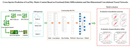
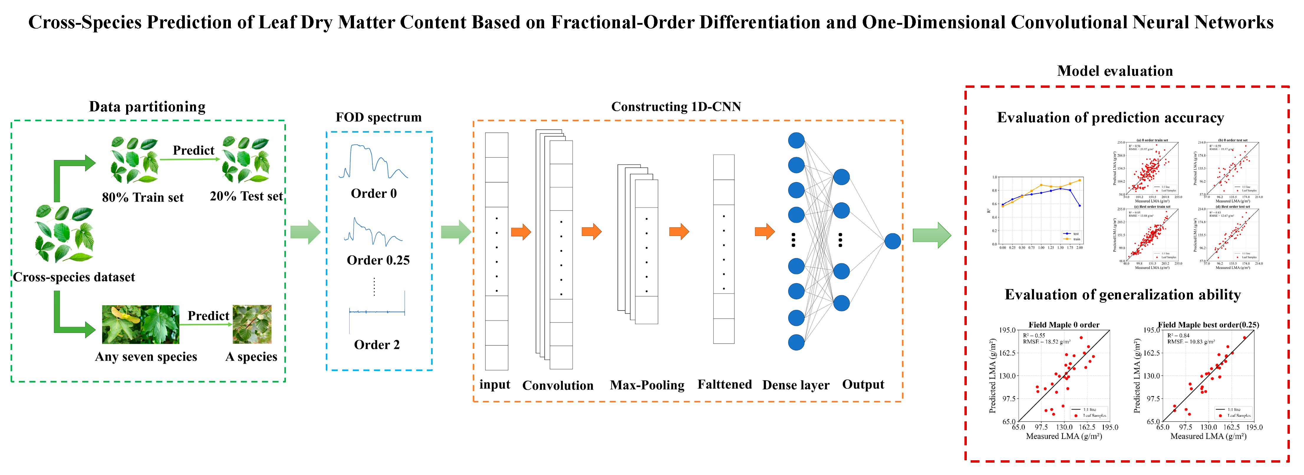
The construction of the proposed 1D-CNN model integrated with FOD spectra in this study consists of two steps. First, the spectral data were preprocessed using FOD with orders from 0 to 2 in steps of 0.25. Second, the 1D-CNN model was designed based on the AlexNet architecture. Figure 1 illustrates the workflow of the proposed method in this study. The CNN model used in this study was implemented in Python with the PyTorch framework. It was run on a GPU platform with Ubuntu 24.04.3 LTS, equipped with an Intel® Xeon® CPU E5-2609 v4 @ 1.70 GHz, 16 GB DDR4 (2667 MHz) memory, and an NVIDIA GeForce GTX 1080 Ti graphics card. The software environment included Python 3.12.8, PyTorch 2.5.0, and CUDA 12.4.
Figure 1.
The workflow of the proposed method.
2.2.1. Fractional-Order Spectral Derivative Algorithm
In this study, a Fourier transform-based FOD method was employed to obtain additional information from the hyperspectral data. This method is more flexible than traditional integer-order derivatives [43]. It not only highlights the changing trend of the spectra but also better preserves the important features related to LMA [44].
The theoretical foundation of FOD stems from the equivalent representation of derivatives in the Fourier domain [45]. For a function defined in the wavelength domain, its Fourier transform is denoted as . The integer-order derivatives in the Fourier domain can be expressed as the product of the spectrum and . When the derivative order is extended from an integer to a real number , the Fourier-domain definition of fractional-order derivatives is obtained as shown in Equation (1).
Here, denotes the FOD of the function with order which can be a non-integer. The result is restored to the wavelength domain via the inverse Fourier transform.
In terms of frequency response, the core of the FOD is to apply an amplification factor of magnitude to each frequency component [46].
This amplification factor determines the degree of enhancement of different frequency components during the transformation process. As α increases, high-frequency components are amplified more strongly, helping to highlight spectral details; when α is small, low-frequency components dominate, thus smoothing the spectrum and reducing noise. Therefore, the fractional-order parameter α is the sole core control parameter of the FOD method, allowing continuous adjustment from smoothing to sharpening [47].
In practical calculations, hyperspectral data are represented as discrete spectra sampled at equal band intervals. FOD is implemented in the frequency domain using the Fast Fourier Transform (FFT) and then recovered to the original wavelength domain using the inverse Fourier transform. Since a small imaginary component may be introduced during numerical calculations, only the real part of the final result is retained to ensure consistency with the original real-valued spectrum. Compared to traditional difference methods, FOD does not rely on a sliding window, thereby avoiding boundary errors and numerical instability [48]. Moreover, derivatives of different orders can be flexibly obtained by adjusting the fractional order . In this study, was set to 0, 0.25, 0.5, 0.75, 1, 1.25, 1.5, 1.75, and 2.
2.2.2. Construction of 1D-CNN Model
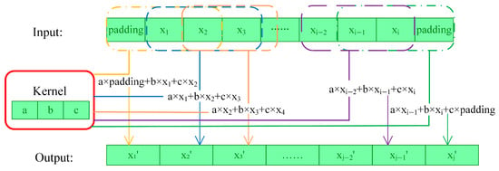
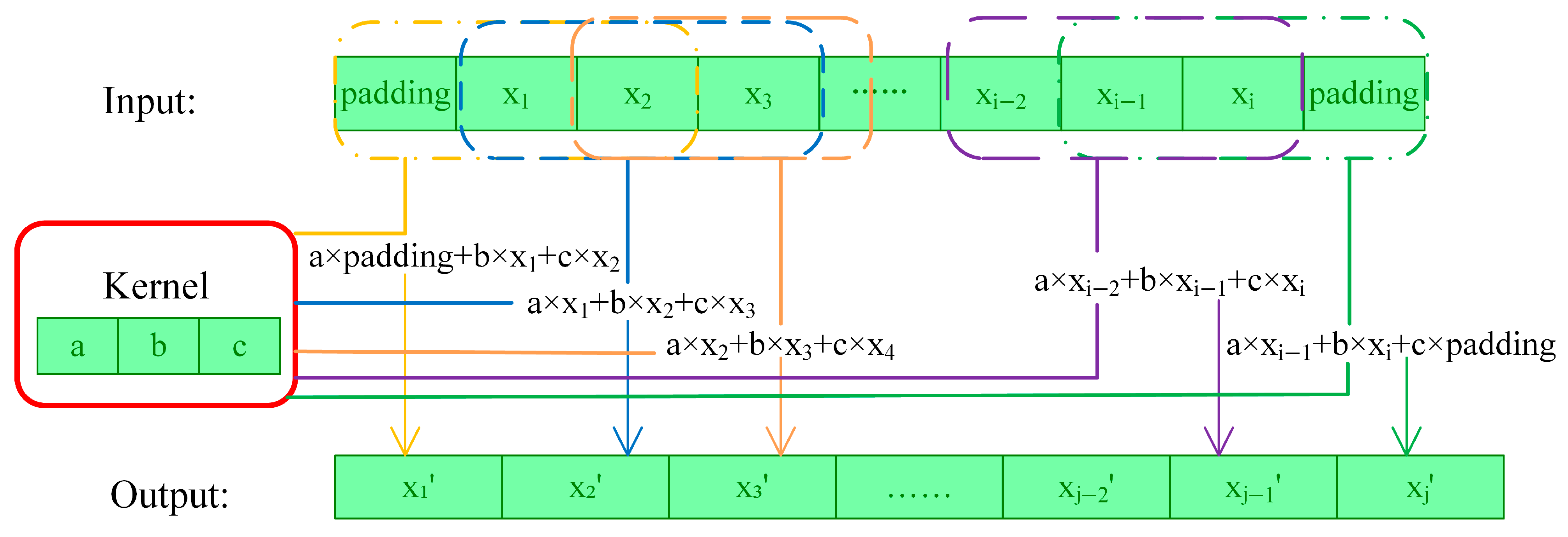
This study aims to predict LMA by constructing a regression model based on a 1D-CNN model. A 1D-CNN model suitable for hyperspectral reflectance is built. Due to its lightweight nature and excellent performance, AlexNet was chosen as the base framework for the proposed model. The input to the model is hyperspectral reflectance corresponding to each sample. The wavelength range of the spectra is 350–2500 nm, with a spectral resolution of 1 nm. Each sample contains 2151 bands. These bands form a one-dimensional array. The spectral data are reshaped into a tensor of size 1 × 2151. The tensor is fed into the model as input. The output of the model is the LMA value corresponding to each sample. Five one-dimensional convolutional layers form the feature extraction module. The numbers of channels for each layer are 96, 256, 384, 384, and 256. There are convolutional kernels with sizes of 11, 5, 3, 3, and 3. Table 1 presents all parameters of the 1D-CNN model and the convolution process is shown in Figure 2.
Table 1.
All parameters of the proposed 1D-CNN model.
Figure 2.
The process of one-dimensional convolution. (Each color used in the figure represents a single convolution sliding window and its corresponding output position).
Each convolutional layer is followed by the ReLU activation function. The computation of ReLU is expressed by Equation (3).
Max-pooling layers are added following the first two convolutional layers and the third convolutional layer. Max-pooling layer is used to perform downsampling. This aids in reducing the feature map size. The feature maps output by the convolutional layers are flattened. The flattened features are input into two fully connected layers. Each fully connected layer contains 4096 neurons. Dropout layers are inserted between each fully connected layer to prevent overfitting. The fully connected module is used to integrate high-level features. Finally, we predict the LMA by a linear output node. The loss function used is the mean squared error (MSE). The model parameters are optimized during training to minimize the error between the predicted and actual measured LMA. The MSE loss function is defined by Equation (4).
Here, and represent the actual measured and predicted LMA of the -th sample and denotes the number of all samples.
During model training, GPU acceleration is prioritized for computation, while the CPU is used when the GPU is unavailable. Network parameters are updated using the Adam optimizer with an initial learning rate of 1 × 10⁻⁴, and no learning rate decay strategy is employed during training. The maximum number of training epochs is set to 400, and the batch size is fixed at 32.
2.3. Model Evaluation and Comparison
2.3.1. Experimental Strategies
This study assesses how well the model predicts LMA and generalizes across different species. The evaluation is conducted from two aspects. On the one hand, all samples are randomly divided into training and test subsets with an 8:2 split to assess the model’s prediction performance on the entire dataset. On the other hand, the model’s generalization is tested by examining its prediction performance on species not included in the training set. A dataset including eight different species is used in this study. In every experiment, a single species is chosen for testing, while the other seven species serve as the training dataset. Based on this selection strategy, eight experimental strategies are designed as shown in Table 2.
Table 2.
Experimental strategies for cross-species generalization evaluation.
2.3.2. Model Evaluation Metrics
Model performance was quantitatively assessed using the coefficient of determination (R2) and the root mean square error (RMSE), two standard metrics frequently employed in regression analysis. R2 focuses on assessing the fit quality.
Here, represents the actual measured LMA, denotes the predicted LMA, and stands for the mean of the actual measured LMA.
RMSE measures the difference between the model-predicted LMA and the observed LMA. RMSE indicates how accurately the model predicts values. A lower RMSE value indicates a smaller prediction error of the model.
Here, represents the actual measured LMA, denotes the predicted LMA, and n stands for the number of leaf samples.
2.3.3. Model Comparison
To assess the prediction capability of the proposed 1D-CNN model, three machine-learning methods were used for comparison, including PLSR, RF, and SVR. PLSR is widely applied in the prediction task between spectra and LMA. It can perform feature extraction and dimensionality reduction. This makes it especially suitable for scenarios with limited sample size but high-dimensional spectral data [49]. RF is a powerful ensemble learning algorithm that can effectively model complex nonlinear relationships. It is also stable against input noise and outliers. In many studies, RF has been widely applied to the inversion of remote sensing data to predict LMA. It has shown stable and high-precision performance [50,51]. Using a kernel function, SVR transforms spectral data into a multidimensional feature space. This enables it to capture nonlinear associations between spectral data and the predicted variable while mitigating the impact of outliers. It has long been recognized as an effective method for nonlinear spectral modeling [52]. In this study, the PLSR, RF, and SVR models were configured with fixed and representative hyperparameters. This ensures a fair comparison of model performance on datasets with different fractional derivatives. The PLSR model was configured with two latent variables. The RF model consisted of 100 decision trees with a maximum depth of 5. The SVR model used a radial basis function (RBF) kernel to capture the nonlinear relationship between spectral features and the target variable, with a penalty parameter C of 100, an adaptive kernel width, and an ε-insensitive loss parameter of 0.2.
This study processes spectra using FOD and splits data 8:2 into training and test sets. All machine-learning models are trained. The best test performance of each model across orders is selected and compared with 1D-CNN at its optimal order to evaluate prediction accuracy. Then, data are divided by species to assess generalization. Models are trained and tested following the strategies in Table 2. The best performance of each traditional model under each strategy is compared with the 1D-CNN results. This comparison enables the evaluation of 1D-CNN’s cross-species generalization ability.
3. Results
3.1. Statistical Analysis of LMA Across Species
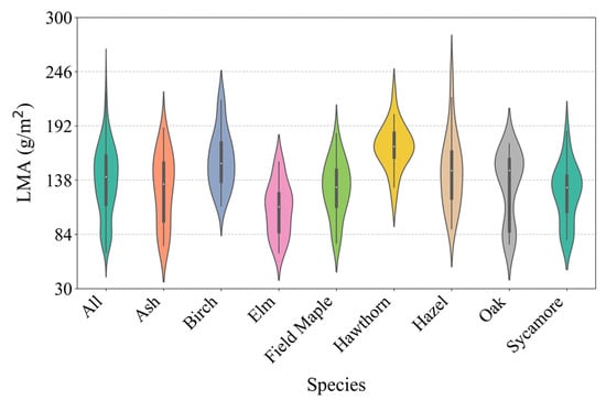
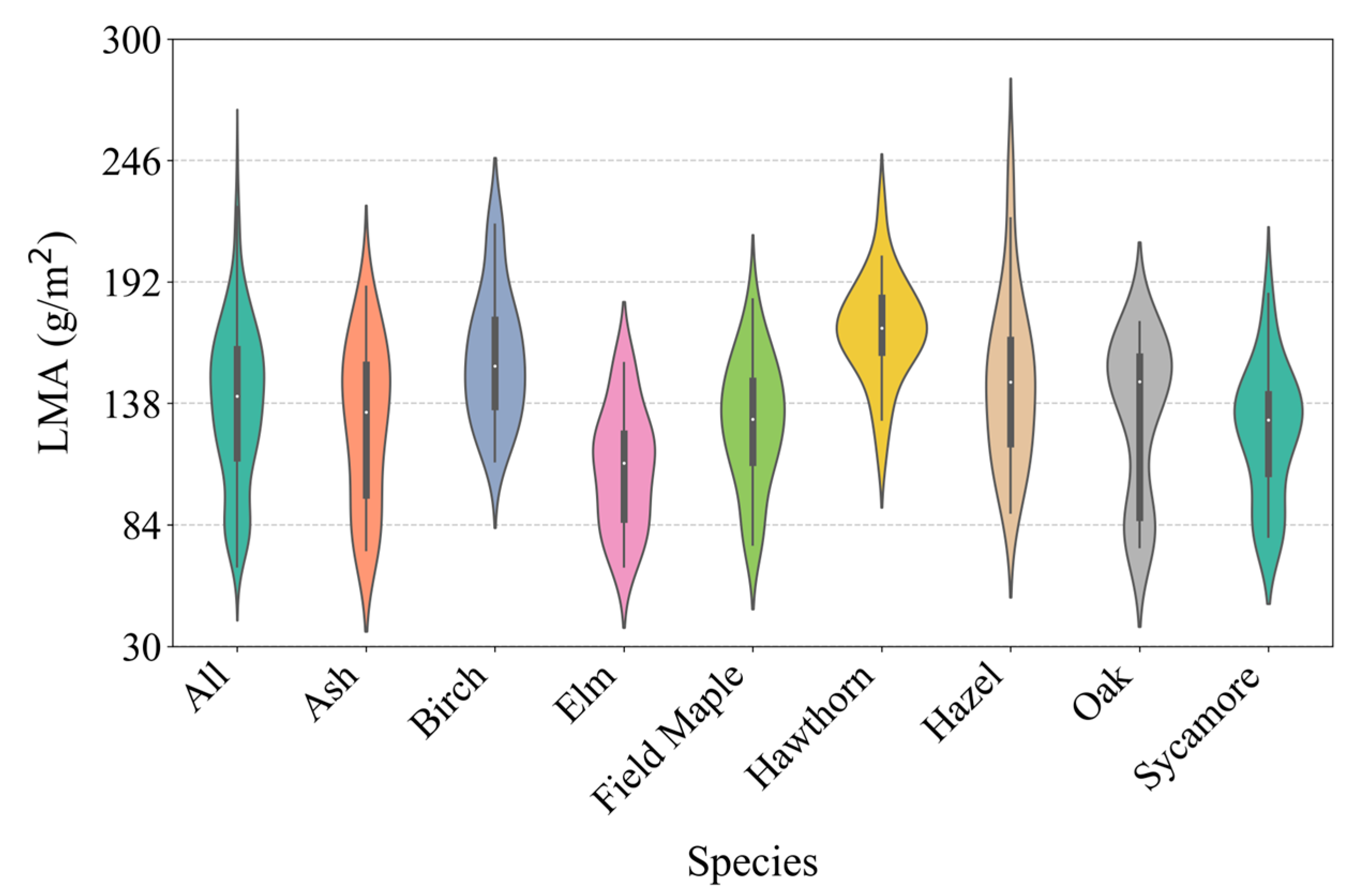
Table 3 summarizes the statistical characteristics of the LMA of different tree species, including sample size, minimum, maximum, mean, median, and standard deviation. Figure 3 shows the distribution of LMA across different species. The overall dataset contained 224 samples, with 28 samples for each species. The overall LMA ranged from 65.46 to 244.68 g/m2, indicating significant differences in LMA among different tree species.
Table 3.
Statistical characteristics of LMA for all samples across species.
Figure 3.
Violin plots of LMA distributions across species. “All” represents the entire set of samples combined from all species.
From the perspective of LMA distributions, the lower and upper bounds of LMA differed markedly among tree species. The minimum LMA was lowest in Elm at 65.46 g/m2 and highest in Hawthorn at 115.10 g/m2, corresponding to an approximately 1.76-fold difference. The minimum LMA values for Elm, Ash, Oak, Field Maple, and Sycamore fell within the range of 65.46–78.64 g/m2. In contrast, the minimum values for Hazel, Birch, and Hawthorn were all above 89.52 g/m2, indicating significantly higher lower bounds of LMA. Regarding maximum values, Hazel showed the highest LMA at 244.68 g/m2 and Elm the lowest at 155.98 g/m2, with an approximate 1.57-fold difference. Hazel, Hawthorn, and Birch all exhibited maximum LMA values exceeding 217 g/m2.
In terms of mean and median, Hawthorn had the highest average LMA at 171.04 g/m2, while Elm had the lowest at only 109.24 g/m2. Based on average values, tree species can be divided into three groups: the high-LMA group included Hawthorn and Birch, with an average LMA of no less than 158 g/m2; the medium-LMA group included Hazel, Oak, Ash, Field Maple, and Sycamore, with average values mainly ranging from 124.99 to 144.67 g/m2; and the low-LMA group included only Elm. The Hawthorn distribution showed a very small difference between its mean and median, indicating a nearly symmetrical distribution. In contrast, the Birch distribution had a median slightly lower than its mean, suggesting a slight right skewness. In terms of dispersion, Hazel exhibited the largest standard deviation, reaching 35.87 g/m2, whereas Hawthorn showed a lower standard deviation of 22.72 g/m2. By comparison, the standard deviations of Hawthorn, Elm, and Sycamore were all no greater than 26.99 g/m2, indicating relatively concentrated LMA distributions.
3.2. Analysis of FOD Spectra
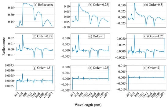
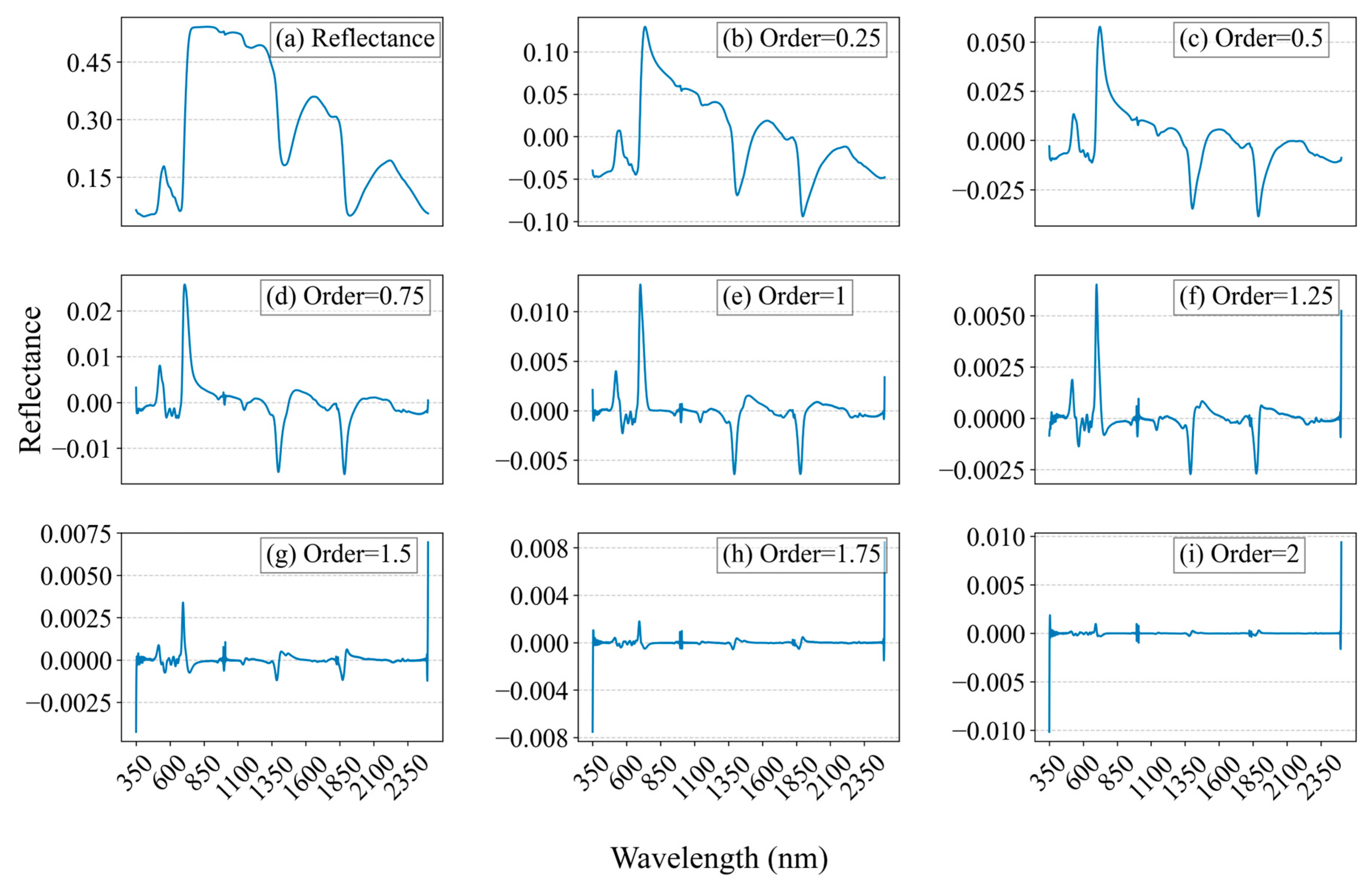
To explore the performance of the FOD algorithm, FOD ranging from 0 to 2 orders at 0.25 steps was applied to raw spectra, as shown in Figure 4. The study found that the 0 order spectra exhibited distinct reflectance peaks and two absorption troughs in the NIR and SWIR regions. When the derivative order ranged from 0.75 to 1.25, these three reflectance peaks and two absorption troughs in the NIR and SWIR regions became sharper and more pronounced. As the order increased to between 1.5 and 2.0, these peaks and troughs gradually weakened and eventually disappeared. Specifically, the reflectance of the 0-order derivative spectra peaked at 750 nm and 1660 nm, with troughs at 700, 1450, and 1950 nm. At the 0.25 order, the first peak sharpened and trough differences decreased. At the 0.5–1.25 orders, the first peak and troughs sharpened further. At the 1.5–2 orders, most features weakened, leaving spectra nearly flat except at 350 nm and 2500 nm.
Figure 4.
FOD spectra at different orders. Derivative orders are incremented from 0 to 2 in steps of 0.25. The blue curve denotes the mean spectra derived from all samples.
3.3. Correlation Analysis Between FOD and LMA
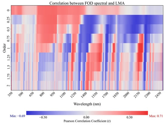
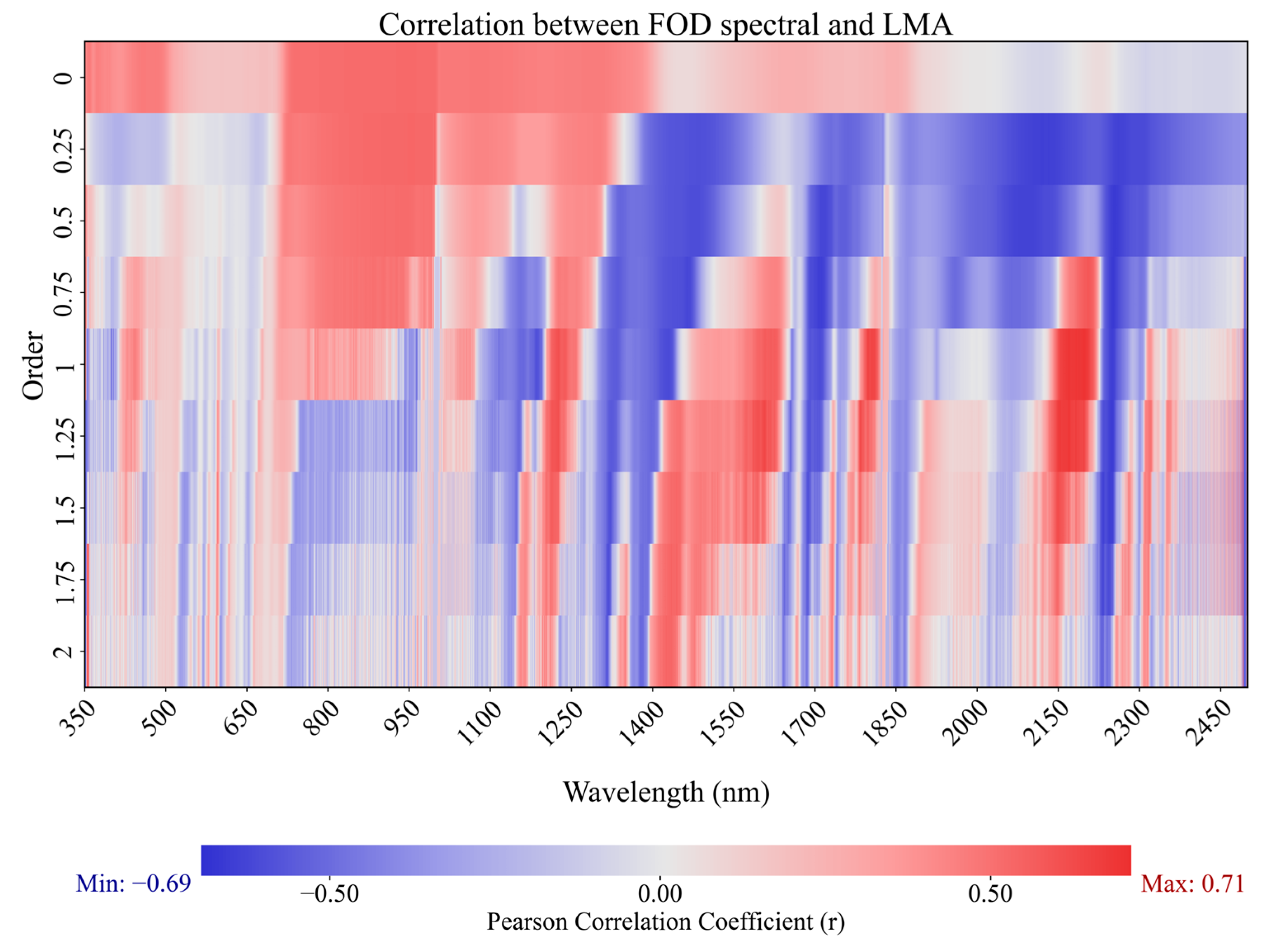
The Pearson correlation coefficients (r) between FOD spectra and LMA were calculated and are presented as a heatmap in Figure 5. The spectral range was 350–2500 nm. The FOD orders ranged from 0 to 2 with a step size of 0.25. The results showed that as the derivative order increased, the overall correlation with LMA gradually strengthened and the high-correlation spectral regions became more scattered.
Figure 5.
Pearson correlation heat map between LMA and FOD spectra across different derivative orders.
Specifically, under the 0 order, r ranged from −0.09 to 0.52, with strong correlations in 350–500 nm and 750–1300 nm. Increasing the order to 0.25–0.75 enhanced negative correlations and revealed alternating positive and negative bands, especially in 800–1000 nm and 2100–2250 nm. At the 1–1.5 orders, the results showed the greatest variety of correlations, with strong positive bands near 1800 and 2250 nm and negative bands near 1650 and 2250 nm. When the order was 1.75–2, the range of r narrowed to −0.57 to 0.61. The positive correlations decreased.
3.4. Prediction Accuracy of the 1D-CNN Model
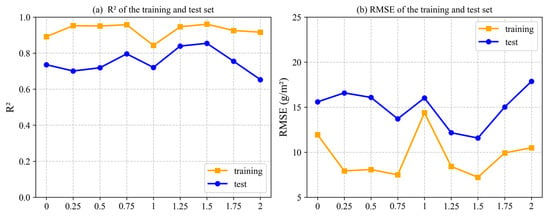
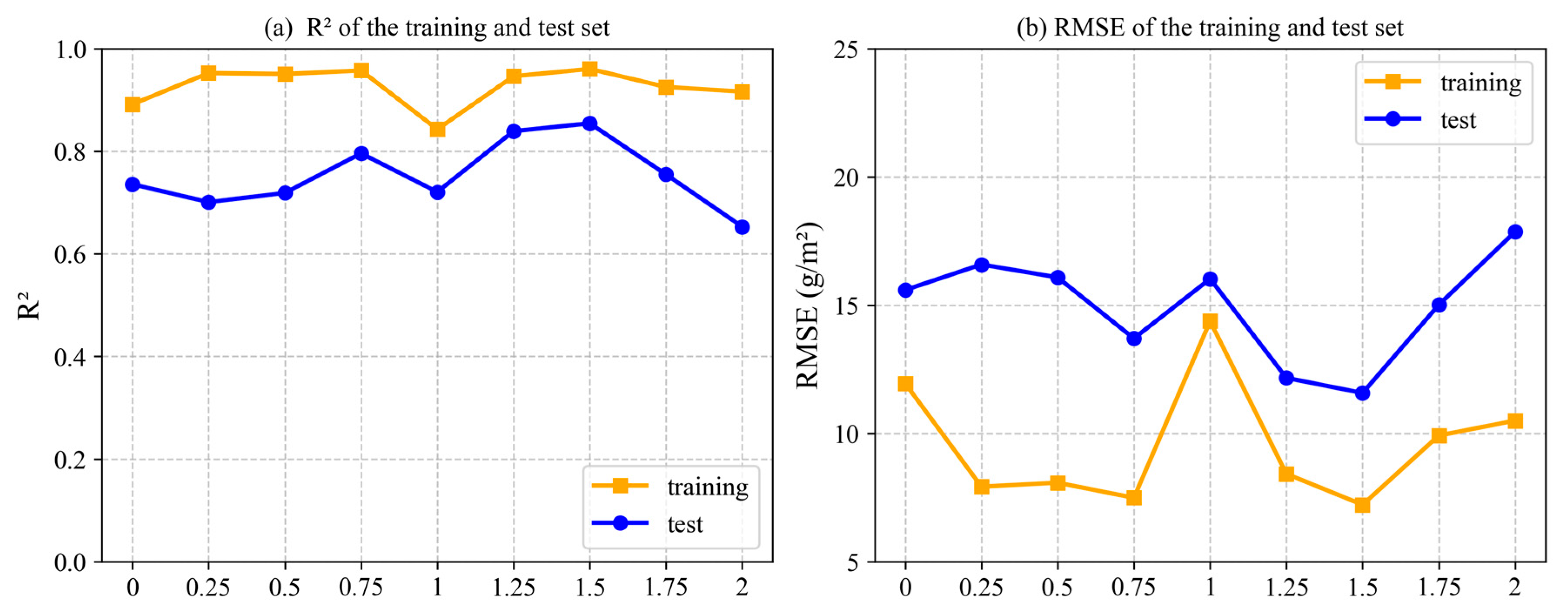
The prediction accuracy of 1D-CNN model was investigated in the 0–2 orders and is illustrated in Figure 6. The trend of R2 with respect to increasing FOD order is presented in panel (a). For the training set, R2 generally rose, dropping at the 1 order and peaking at the 1.5 order. For the test set, R2 increased with minor fluctuations, reaching a maximum at the 1.5 order before declining. RMSE in training gradually decreased, fluctuated around the 1 order, then minimized at the 1.5 order. In testing, RMSE slightly rose, decreased at the 0.75 order, increased at the 1 order, reached a minimum at the 1.5 order, and then increased, showing FOD’s impact on prediction accuracy. These results indicated that FOD processing markedly improved model prediction, with the greatest enhancement observed at the 1.5 order. Compared to conventional integer-order derivatives, FOD provided better prediction accuracy for LMA. Considering both R2 and RMSE, the 1.5 order was identified as the best FOD order for the 1D-CNN model.
Figure 6.
Prediction accuracy of the 1D-CNN model on FOD spectra in 0–2 orders.
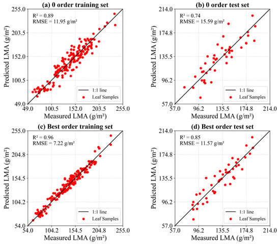
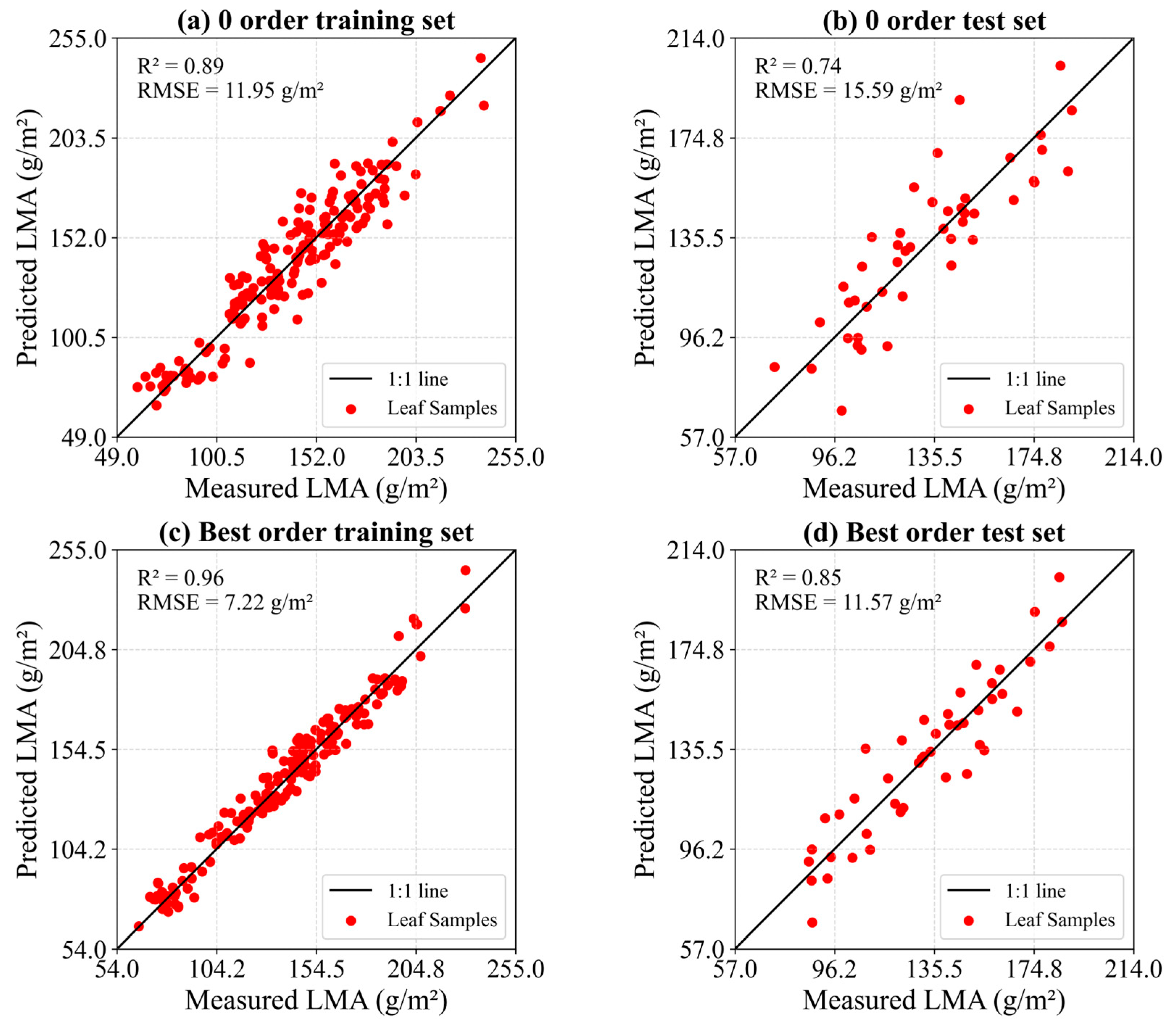
Figure 7 shows scatter plots of predicted versus measured LMA under the 0 and optimal (1.5) orders. At the 0 order, the model showed an R2 of 0.89 for training and 0.74 for testing, accompanied by an RMSE of 11.95 g/m2 and 15.59 g/m2. The application of the 1.5 order improved R2 to 0.96 for training and 0.85 for testing, with the corresponding RMSEs dropping to 7.22 g/m2 and 11.57 g/m2. The application of the 1.5 order led to predicted value aligning more closely with the 1:1 line, reflecting better concordance between predicted and measured LMA. The model accuracy was clearly improved, and the prediction results at the 1.5 order were significantly better than those at the 0 order.
Figure 7.
Scatter plots of measured vs. predicted LMA for the 1D-CNN model on training and test sets at 0 order and the best order (1.5 order).
3.5. Generalization Performance of the 1D-CNN Model
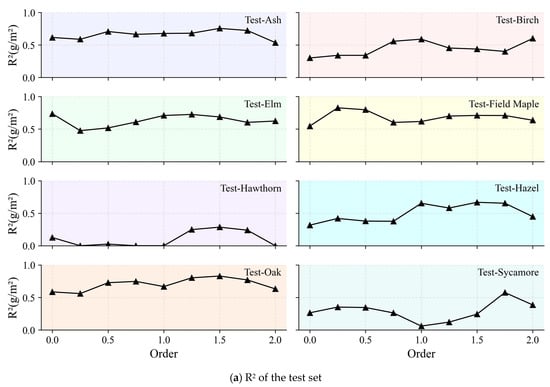
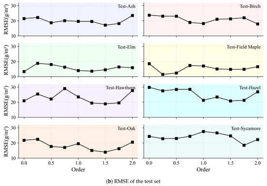
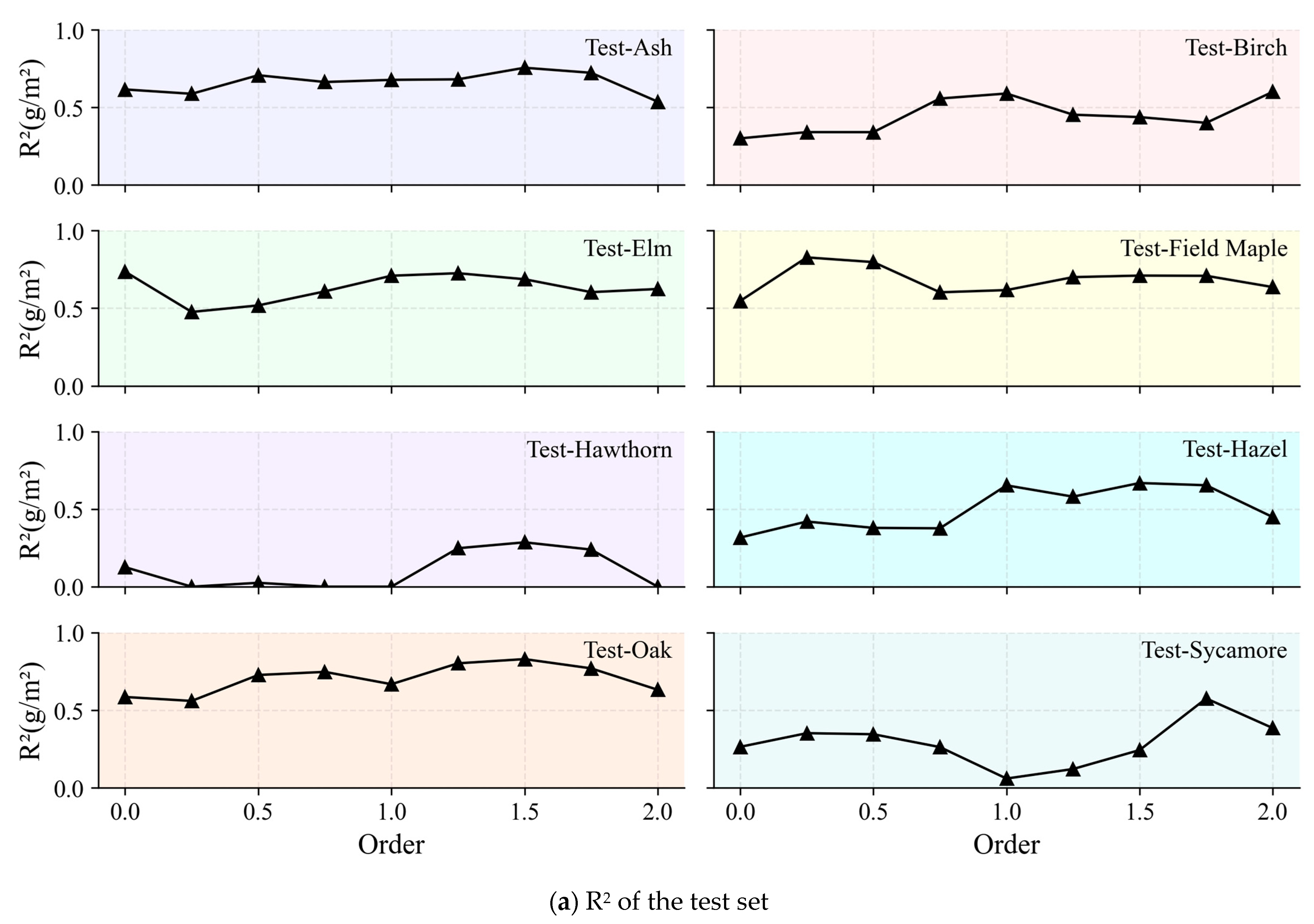
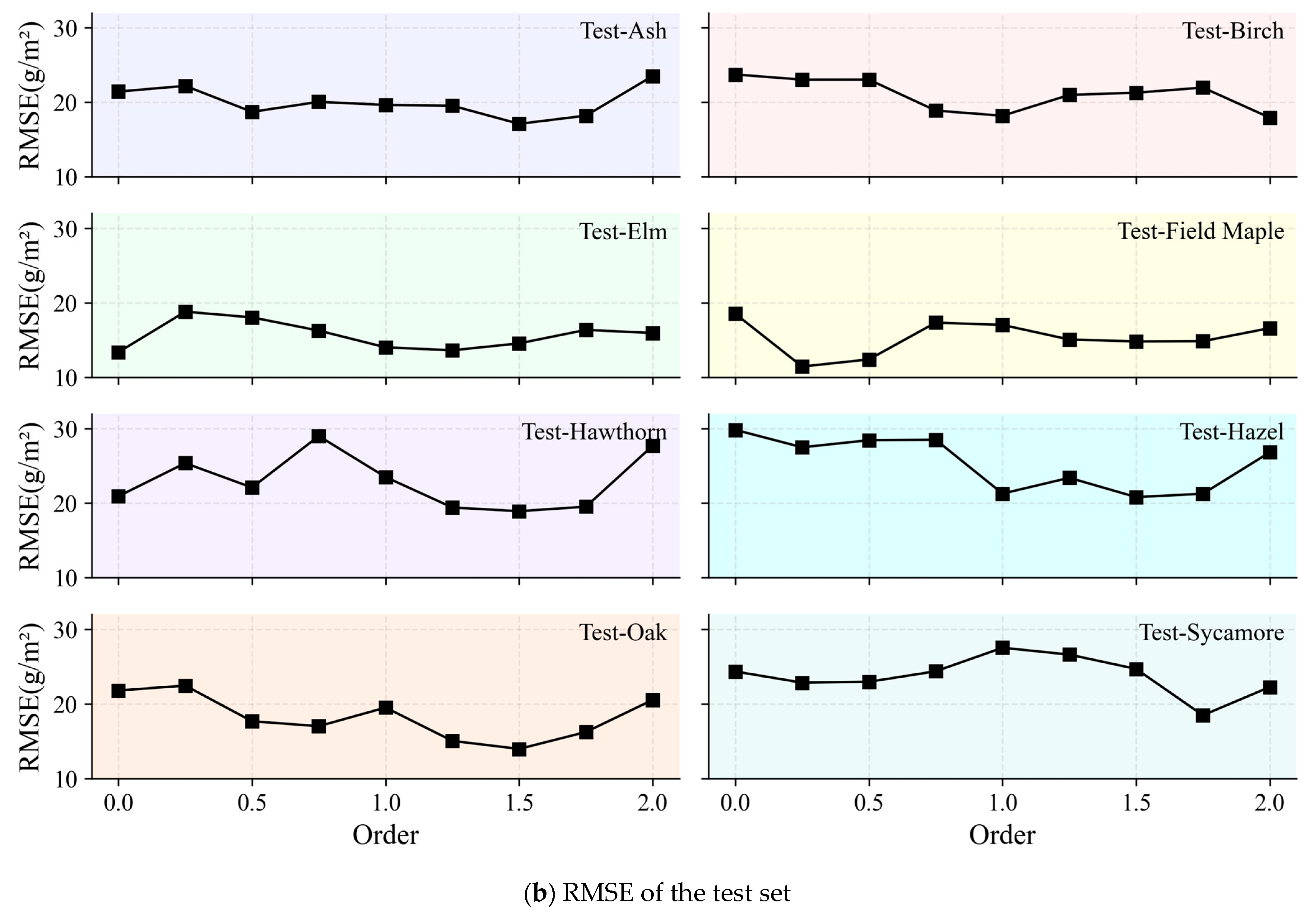
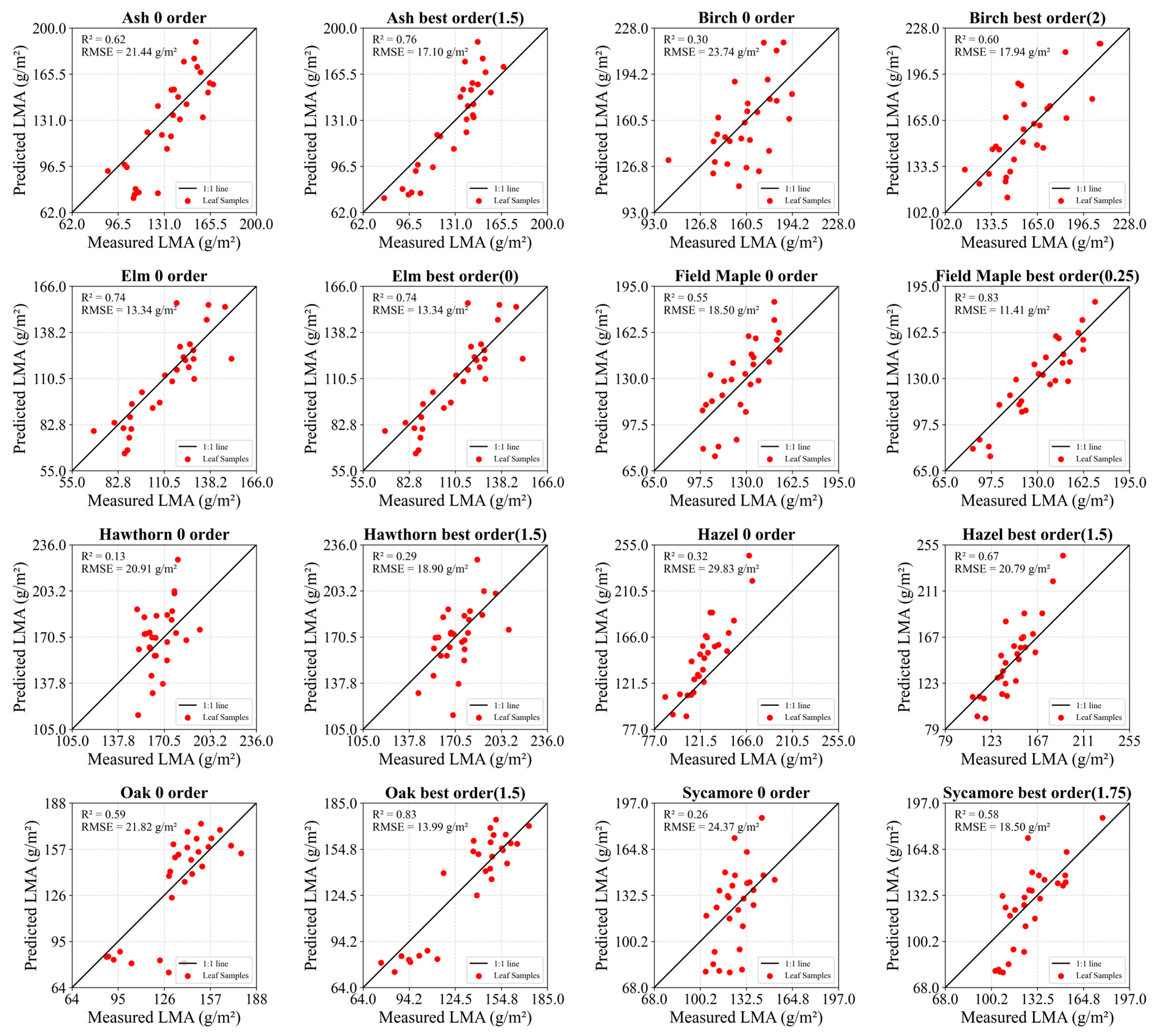
To evaluate the generalization performance of the 1D-CNN model, the results of eight experimental strategies are presented in Figure 8 and Figure 9. The figures show that FOD enhanced model performance. For the seven experimental strategies excluding Test-Elm, prediction accuracy at the best order outperformed that under the 0 order. In the Test-Elm experimental strategy, the prediction accuracy at the 0 order was the highest, but only slightly better than that at the 1.25 order.
Figure 8.
Prediction results of the 1D-CNN with FOD spectra for eight experimental strategies. (a) R2 of the test set. (b) RMSE of the test set.
Figure 9.
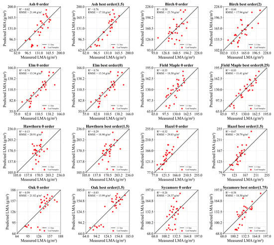
Scatter plots of measured and predicted LMA for eight experimental strategies at the 0 order and the best order. The species above each subplot represent the predicted species, with the optimal order given in parentheses (e.g., “Ash 0 order” indicates the Test-Ash strategy under the 0 order).
Among all strategies, Test-Ash, Test-Elm, Test-Field Maple, and Test-Oak showed particularly strong results. In Test-Ash, the model achieved its best performance at the 1.5 order. The R2 increased to 0.76 and the RMSE dropped to 17.10 g/m2. When the order was 0, the model’s prediction results showed an R2 of 0.62 and an RMSE of 21.44 g/m2. Compared to the 0 order, the 1.5 order improved R2 by 0.14 and reduced RMSE by 4.34 g/m2. In Test-Elm, the best result was obtained at the 0 order. The R2 reached 0.74 and the RMSE was 13.34 g/m2. The R2 was 0.73 and the RMSE was 13.60 g/m2 at the 1.25 order. The model’s prediction result at the 0 order was only 0.01 higher than that at the 1.25 order, and their RMSE values were also very close. The highest predictive accuracy for Test-Field Maple was obtained at the 0.25 order. The R2 rose to 0.83 and the RMSE decreased to 11.41 g/m2. Compared to the 0 order, the model at the 0.25 order showed an improvement of 0.28 in R2 and a reduction of 7.09 g/m2 in RMSE. In Test-Oak, the best result occurred at the 1.5 order. The R2 improved to 0.83 and the RMSE dropped to 13.99 g/m2. Compared to the model performance at the 0 order, the model at the 1.5 order improved by 0.24 in R2 and reduced RMSE by 7.83 g/m2.
3.6. Prediction Accuracy of the Comparison Models
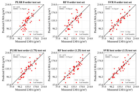
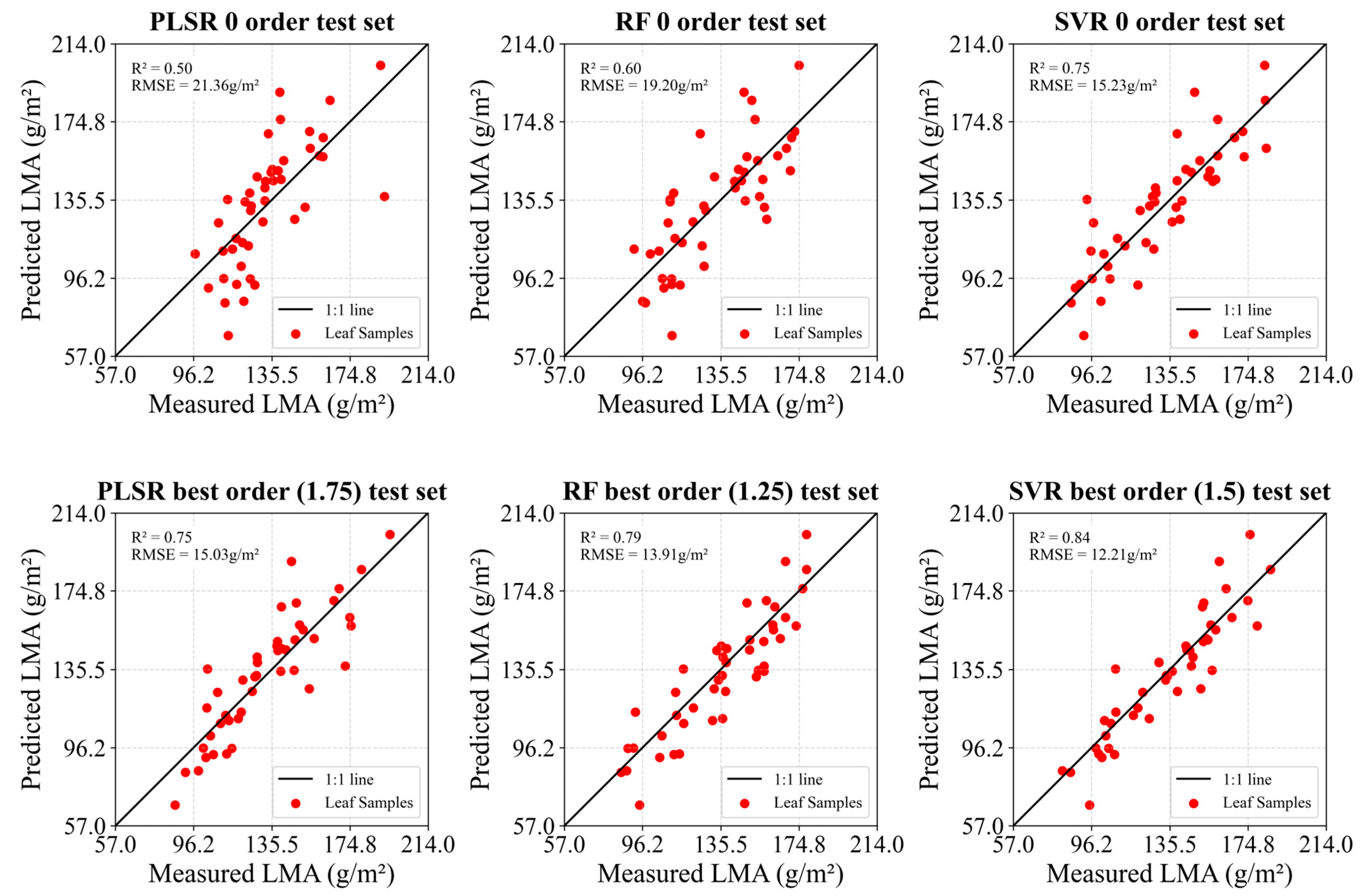
Figure 10 presents scatterplots of predicted and measured LMA on the test set for three machine-learning models (PLSR, RF, and SVR). In the figure, the results for each model at the 0 order and their best orders are arranged from top to bottom, with different models displayed from left to right.
Figure 10.
Scatter plots of measured and predicted LMA for the 0 order and the optimal orders in the PLSR, RF, and SVR models. The corresponding optimal order is indicated in brackets.
At the 0 order, SVR achieved the best prediction performance on the test set, with an R2 of 0.75 and an RMSE of 15.23 g/m2. The test set results for PLSR showed an R2 of 0.50 and an RMSE of 21.36 g/m2, whereas RF achieved an R2 of 0.60 with an RMSE of 19.20 g/m2. That indicated that SVR had the highest predictive accuracy without differential processing. All models showed improvement at their best orders. Among the traditional models, SVR achieved the best performance at the 1.5 order, with an R2 of 0.84 and an RMSE of 12.21 g/m2. Nevertheless, the proposed 1D-CNN model outperformed all compared models, with an R2 of 0.85 and an RMSE of 11.57 g/m2 on the test set at the best order of 1.5, which demonstrated better accuracy. Although R2 was only 0.01 higher than SVR, the scatter plot showed that SVR had an obvious overestimation at high values.
3.7. Generalization Performance of Comparison Models
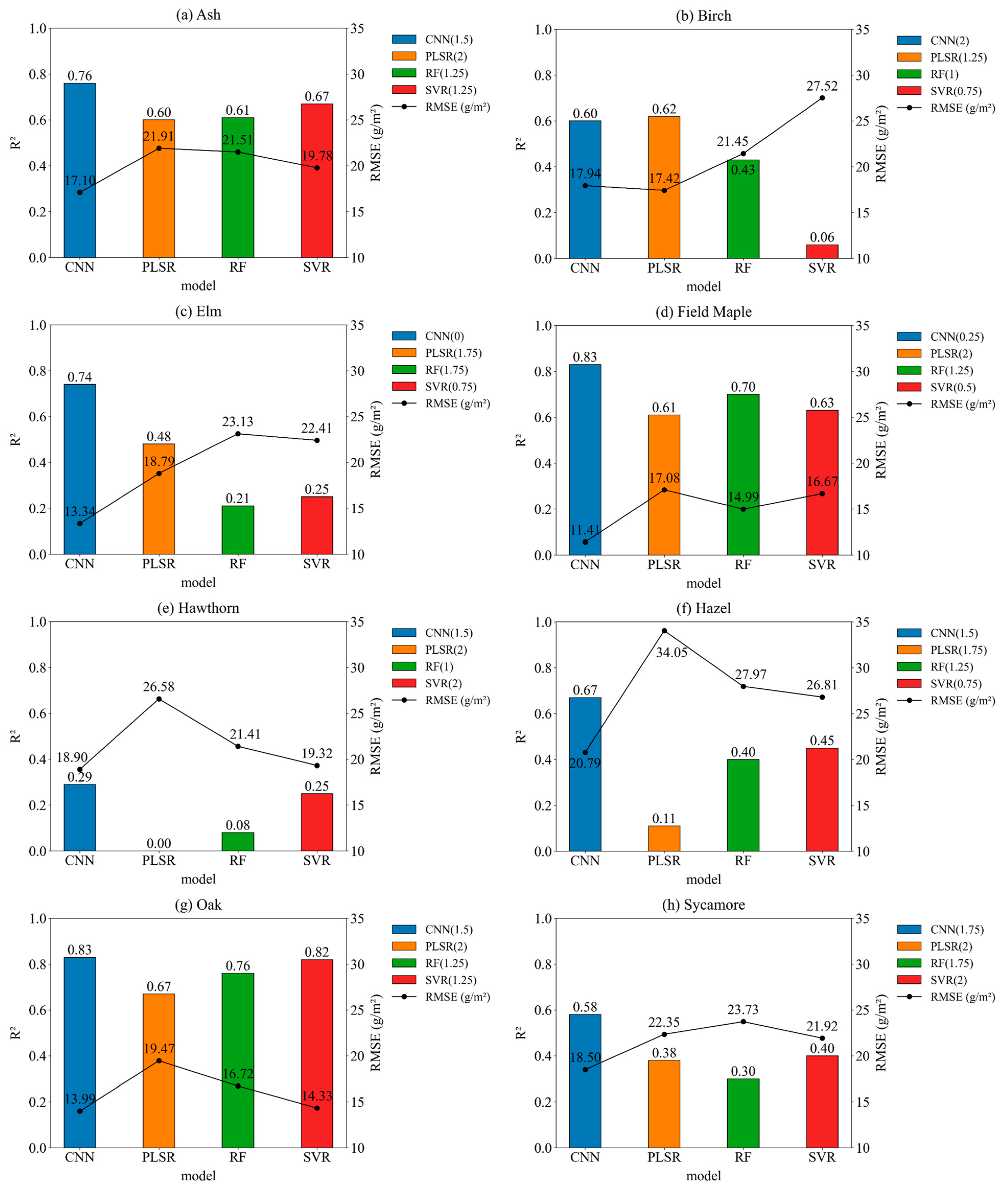
In terms of generalization performance, the 1D-CNN model was compared with PLSR, RF, and SVR by predicting cross-species LMA, as shown in Figure 11. The 1D-CNN model displays improved generalization capability.
Figure 11.
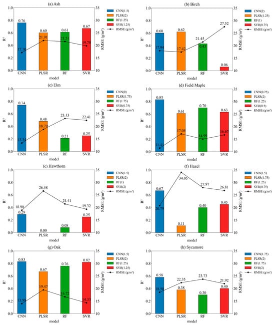
R2 and RMSE of 1D-CNN, PLSR, RF, and SVR models under eight experimental strategies for LMA prediction. Each subplot represents one experimental strategy (e.g., Ash denotes the Test-Ash strategy). The legend in the upper right indicates the model names and the optimal order for each strategy.
Among the eight cross-species experiments, CNN significantly outperformed all traditional models in seven groups: Test-Ash, Test-Elm, Test-Field Maple, Test-Hawthorn, Test-Hazel, Test-Oak, and Test-Sycamore. In Test-Ash, the best predictive performance of CNN was an R2 of 0.76 and an RMSE of 17.10 g/m2, while SVR achieved an R2 of 0.67 and an RMSE of 19.78 g/m2. CNN performed better than SVR. In Test-Elm, CNN achieved its best performance with an R2 of 0.74 and an RMSE of 13.34 g/m2, whereas PLSR reached an R2 of 0.48 and an RMSE of 18.79 g/m2. CNN outperformed PLSR. In Test-Field Maple, the best predictive performance of CNN was an R2 of 0.83 and an RMSE of 11.41 g/m2. RF achieved an R2 of 0.70 and an RMSE of 14.99 g/m2. CNN performed better than RF. CNN also showed higher accuracy in Test-Hawthorn, Test-Hazel, Test-Oak, and Test-Sycamore. In the remaining group, although CNN did not always achieve the highest accuracy, it still demonstrated a stable performance. In Test-Birch, CNN achieved a best predictive performance with an R2 of 0.58 and an RMSE of 18.43 g/m2, while PLSR achieved an R2 of 0.62 and an RMSE of 17.42 g/m2. PLSR performed slightly better than CNN.
3.8. Sensitive Bands for Different Species
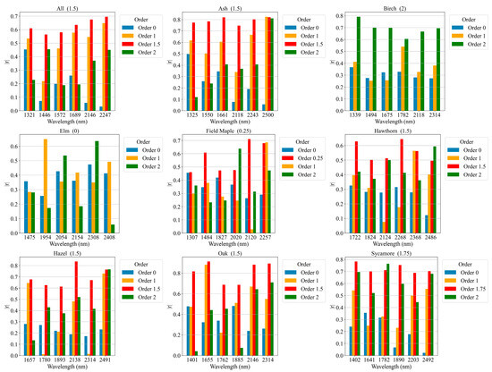
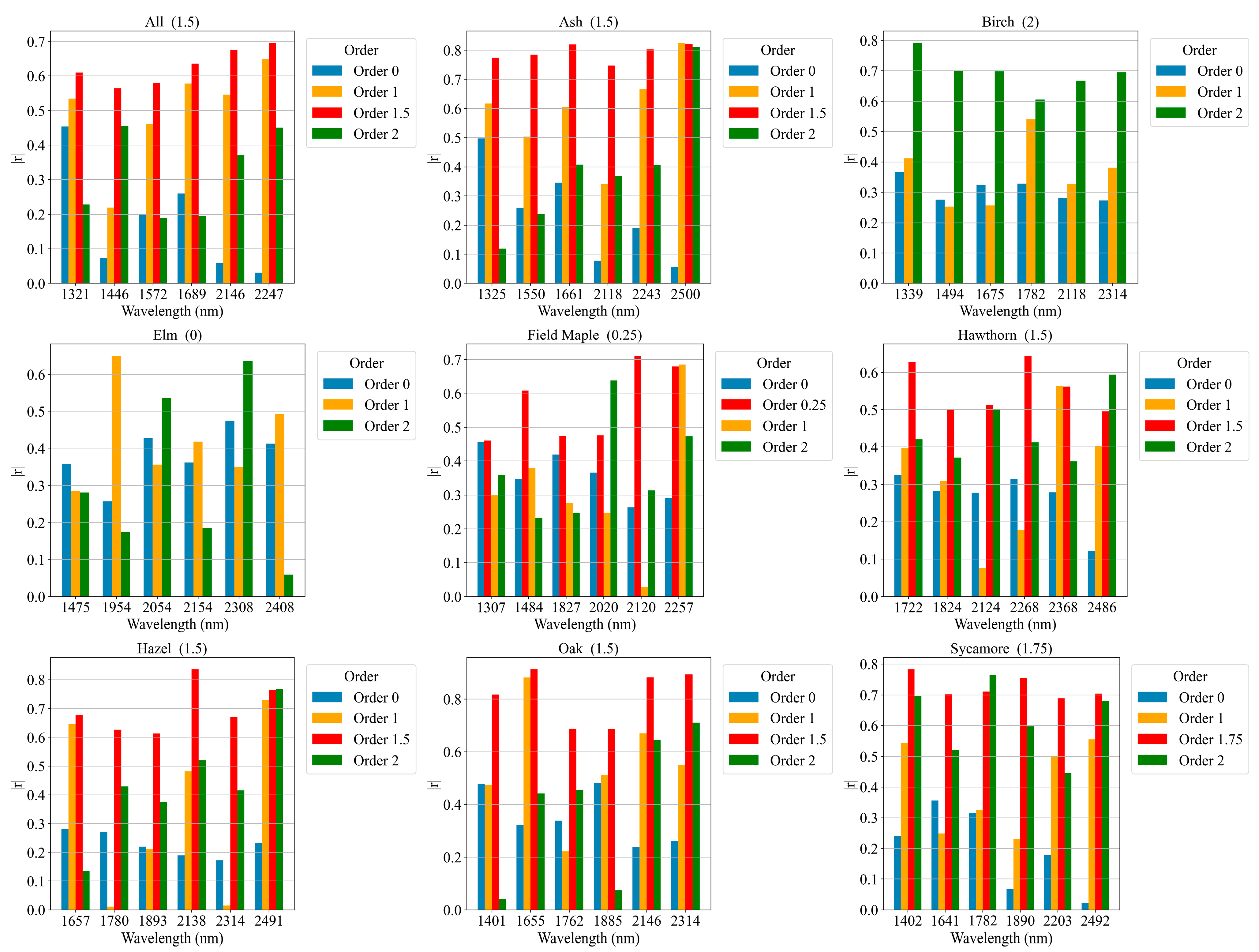
In this study, sensitive bands were extracted from the entire dataset as well as from each species. The absolute Pearson correlation coefficients (|r|) linking spectral reflectance and LMA were calculated for the best order and integer orders (0, 1, and 2). The identified sensitive bands were illustrated in Figure 12. Applying FOD processing notably increased the correlation between spectral reflectance and LMA in the sensitive bands, as shown in Figure 12. For the entire dataset, the best order was 1.5, with |r| values in six sensitive bands (1321, 1446, 1572, 1689, 2146, 2247 nm) ranging from 0.56 to 0.69, all higher than integer orders. Similar advantages were observed at the species level: in Oak, all sensitive bands had a higher |r| at the best order; in Ash, Hazel, and Sycamore, five bands showed the same; and in Field Maple and Hawthorn, four bands did.
Figure 12.
Bar graphs of the absolute Pearson correlation coefficients (|r|) between FOD sensitive bands and LMA for the entire dataset (All) and individual species. Each subplot title indicates the predicted species and its optimal order (e.g., All (1.5) for the entire dataset, Ash (1.5) for the Ash species in the Test-Ash strategy).
4. Discussion
4.1. Effectiveness of FOD for LMA Prediction
FOD with appropriate orders could better enhance important spectral information and effectively suppress noise than traditional first- or second-order derivatives [53]. This study demonstrated that FOD-processed hyperspectral data outperformed traditional integer-order derivatives in terms of LMA prediction. The 1.5-order derivative processing achieved the best accuracy (R2 = 0.85, RMSE = 11.57 g/m2), surpassing first- and second-order preprocessing. The optimal order varied by models and datasets. For the 1D-CNN model, the optimal derivative order was 1.5 for the entire dataset, whereas orders of 0.25 and 1.75 were optimal for Test-Field Maple and Test-Sycamore, respectively. PLSR, RF, and SVR achieved their best performance on the entire dataset at derivative orders of 1.75, 1.25, and 1.5, respectively. Several studies have demonstrated that preprocessing hyperspectral data with FOD can improve the prediction accuracy of leaf biochemical parameters [54,55]. Zhuang et al. applied FOD for spectral preprocessing in the prediction of leaf chlorophyll fluorescence parameters, achieving an R2 of approximately 0.71 which was higher than that obtained without FOD [56]. Li et al. showed that FOD-based spectral preprocessing improved the prediction of grape leaf chlorophyll content compared with the original spectra [57].
FOD processing can significantly enhance the correlation between sensitive bands and LMA. Although the sensitive bands vary slightly among different species, their overall distributions are generally consistent. Cheng et al. reported that 1368 nm, 1639 nm, and 2133 nm are particularly sensitive to LMA [19]. In this study, the sensitive bands of Ash, Birch, Oak, and Sycamore were close to 1368 nm and 1629 nm, while the sensitive bands of all eight species were located near 2133 nm. Maire et al. identified 1490 nm and 2260 nm as sensitive bands for LMA [58]. Correspondingly, the sensitive bands of Birch, Elm, and Field Maple in this study were close to 1490 nm, whereas those of Field Maple and Hawthorn were close to 2260 nm. These sensitive bands are associated with the absorption features of the main biochemical constituents of LMA, including cellulose, lignin, proteins, and starch. The slight differences in sensitive wavelength positions among studies may result from variations in sample types or measurement environments.
4.2. Advantages of FOD-Based 1D-CNN
1D-CNN models have the characteristics of high prediction accuracy and strong generalization ability, which are mainly attributed to its end-to-end automatic feature learning ability [59]. 1D-CNN can automatically extract key local features from hyperspectral data, leverage correlations between adjacent bands, and capture intrinsic multi-scale structures, effectively reducing noise [60]. In addition, the pooling layer integrates information and reduces dimensionality, enhancing robustness, mitigating overfitting, and improving generalization across species and environments [61]. Relying on these strengths, the proposed FOD–1D-CNN framework exhibits clear advantages over traditional LMA prediction approaches in both prediction accuracy and cross-species generalization.
Across the entire dataset, FOD–1D-CNN achieved the best overall performance, with R2 = 0.85 and RMSE = 11.57 g/m2, representing an increase in R2 of up to 10% compared with the baseline methods. In most cross-species experimental strategies (e.g., Test-Ash, Test-Elm, Test-Field Maple, Test-Hawthorn, Test-Hazel, Test-Oak, and Test-Sycamore), FOD–1D-CNN consistently surpassed others. These improvements indicate that the combination of FOD and convolutional feature extraction is better suited to capture key spectral signals of LMA than linear or tree-based models. Previous studies have shown that CNN models outperform traditional machine-learning models in predicting leaf biochemical parameters [62,63,64,65]. For example, the study by Wang et al. demonstrated that CNN models increased the prediction accuracy of leaf pigment content by 25% compared with traditional machine-learning models [66]. Gallo et al. also reported that CNN models outperformed traditional machine-learning models in estimating maize canopy nitrogen and chlorophyll content [67]. The results of this study are consistent with previous findings and further demonstrate the advantage of CNN-based models for LMA prediction.
4.3. Limitations and Future Prospects
In this study, the accuracy and generalization performance of FOD–1D-CNN models were specifically investigated in cross-species leaves. This dataset with eight temperate broadleaf woody species spans a wide range of leaf morphologies and LMA values. Thus, it provides a representative sample dataset for evaluating the accuracy and generalization ability of the FOD–1D-CNN model. Cross-species validation was implemented in a leave-one-species-out strategy. The results showed that the FOD–1D-CNN consistently achieved higher R2 and lower RMSE in most experiments, demonstrating its great generalization ability to unseen species. It should be noted that all selected leaf species in this study belong to temperate deciduous broad-leaved trees. Future work should extend to a broader range of vegetation types to further evaluate the model’s generalization ability. The proposed FOD–1D-CNN framework is also promising for extension to airborne and spaceborne hyperspectral images for large-scale LMA mapping.
5. Conclusions
LMA is an important functional trait that is closely associated with plant growth, resource-use efficiency, and ecosystem functioning. While hyperspectral remote sensing offers a non-destructive means of predicting LMA, its application across species is limited by two persistent challenges: low signal specificity due to overlapping biochemical parameters, and limited model performance resulting from spectral variability among species. Aiming to address these challenges, a novel cross-species LMA prediction framework was proposed by integrating FOD with 1D-CNN. This study demonstrated that integrating FOD with 1D-CNN can significantly enhance LMA prediction using hyperspectral data. The 1.5-order derivative achieved the highest accuracy, with R2 = 0.85 and RMSE = 11.57 g/m2, and outperformed both zero-order and integer-order derivatives. The FOD-1D-CNN outperformed traditional machine-learning models (PLSR, RF, and SVR) in both overall accuracy and cross-species generalization. It should be noted that this study only used temperate deciduous broad-leaved species, and future work will extend the proposed FOD–1D-CNN framework to more diverse vegetation types and airborne/spaceborne hyperspectral data for large-scale LMA mapping.
Author Contributions
Conceptualization, L.X., S.S. (Shijie Shan), Q.G., W.J., S.S. (Shuo Shi) and Y.C.; methodology, L.X., S.S. (Shijie Shan) and Q.G.; software, S.S. (Shijie Shan); validation, L.X., Q.G., W.J., S.S. (Shuo Shi) and Y.C.; formal analysis, L.X., S.S. (Shijie Shan) and Q.G.; investigation, L.X., S.S. (Shijie Shan) and Q.G.; resources, L.X., S.S. (Shijie Shan), Q.G., W.J., S.S. (Shuo Shi) and Y.C.; data curation, L.X., S.S. (Shijie Shan) and Q.G.; writing—original draft preparation, L.X. and S.S. (Shijie Shan); writing—review and editing, L.X., S.S. (Shijie Shan), Q.G., W.J., S.S. (Shuo Shi) and Y.C.; visualization, S.S. (Shijie Shan); supervision, L.X., Q.G., W.J., S.S. (Shuo Shi) and Y.C.; project administration, L.X., S.S. (Shuo Shi) and Y.C.; funding acquisition, S.S. (Shijie Shan) and Q.G. All authors have read and agreed to the published version of the manuscript.
Funding
The research was funded by the Technology Research and Development Program of Tianjin (No. 24YDTPJC00060), and the Graduate Student Scientific Research and Innovation Program of Tianjin Chengjian University (No. 2025YKC095).
Data Availability Statement
The original data presented in the study are openly available in FigShare at https://doi.org/10.6084/m9.figshare.16909330.v1 or reference [68].
Acknowledgments
We sincerely acknowledge the open access provided by the following resources: the publicly available dataset, AlexNet, PyTorch, and Python.
Conflicts of Interest
The authors declare no conflicts of interest.
Abbreviations
The following abbreviations are used in this manuscript:
| LMA | Leaf mass per area |
| FOD | Fractional-order derivatives |
| 1D-CNN | One-dimensional convolutional neural network |
| PLSR | Partial least squares regression |
| RF | Random forest |
| SVR | Support vector regression |
| |r| | Absolute Pearson correlation coefficients |
| r | Pearson correlation coefficients |
| R2 | Coefficient of determination |
| RMSE | Root mean square error |
References
- Shi, H.Y.; Jiang, J.Y.; Jacquemoud, S.; Xiao, Z.Q.; Ma, M.G. Estimating leaf mass per area with leaf radiative transfer model. Remote Sens. Environ. 2023, 286, 113444. [Google Scholar] [CrossRef] [Scilit]
- Gara, T.W.; Rahimzadeh-Bajgiran, P.; Darvishzadeh, R. Forest Leaf Mass per Area (LMA) through the Eye of Optical Remote Sensing: A Review and Future Outlook. Remote Sens. 2021, 13, 3352. [Google Scholar] [CrossRef] [Scilit]
- Fei, S.; Xiao, S.; Xu, D.; Shu, M.; Sun, H.; Feng, P.; Xiao, Y.; Ma, Y. Improved random patches and model transfer for deriving leaf mass per area across multispecies from spectral reflectance. Comput. Electron. Agric. 2024, 218, 108745. [Google Scholar] [CrossRef] [Scilit]
- Yang, B.; Lin, H.; He, Y.H. Data-Driven Methods for the Estimation of Leaf Water and Dry Matter Content: Performances, Potential and Limitations. Sensors 2020, 20, 5394. [Google Scholar] [CrossRef] [Scilit]
- Mutanga, O.; Masenyama, A.; Sibanda, M. Spectral saturation in the remote sensing of high-density vegetation traits: A systematic review of progress, challenges, and prospects. ISPRS J. Photogramm. Remote Sens. 2023, 198, 297–309. [Google Scholar] [CrossRef] [Scilit]
- Nardini, A. Hard and tough: The coordination between leaf mechanical resistance and drought tolerance. Flora 2022, 288, 152023. [Google Scholar] [CrossRef] [Scilit]
- Zhang, Y.; Migliavacca, M.; Penuelas, J.; Ju, W. Advances in hyperspectral remote sensing of vegetation traits and functions. Remote Sens. Environ. 2021, 252, 112121. [Google Scholar] [CrossRef] [Scilit]
- Zhang, X.N.; Xu, H.C.; She, Y.H.; Hu, C.; Zhu, T.Z.; Wang, L.L.; Wu, L.Q.; You, C.C.; Ke, J.; Zhang, Q.Q.; et al. Improving the prediction performance of leaf water content by coupling multi-source data with machine learning in rice (Oryza sativa L.). Plant Methods 2024, 20, 48. [Google Scholar] [CrossRef] [Scilit]
- Kothari, S.; Hobbie, S.E.; Cavender-Bares, J. Rapid estimates of leaf litter chemistry using reflectance spectroscopy. Can. J. For. Res. 2024, 54, 978–991. [Google Scholar] [CrossRef] [Scilit]
- Féret, J.B.; le Maire, G.; Jay, S.; Berveiller, D.; Bendoula, R.; Hmimina, G.; Cheraiet, A.; Oliveira, J.C.; Ponzoni, F.J.; Solanki, T.; et al. Estimating leaf mass per area and equivalent water thickness based on leaf optical properties: Potential and limitations of physical modeling and machine learning. Remote Sens. Environ. 2019, 231, 110959. [Google Scholar] [CrossRef] [Scilit]
- Chen, Y.; Sun, J.; Wang, L.; Shi, S.; Gong, W.; Wang, S.; Tagesson, T. Optimized Estimation of Leaf Mass per Area with a 3D Matrix of Vegetation Indices. Remote Sens. 2021, 13, 3761. [Google Scholar] [CrossRef] [Scilit]
- Zhang, Z.C.; Xin, Q.C.; Li, W.J. Machine Learning-Based Modeling of Vegetation Leaf Area Index and Gross Primary Productivity Across North America and Comparison with a Process-Based Model. J. Adv. Model. Earth Syst. 2021, 13, e2021MS002802. [Google Scholar] [CrossRef] [Scilit]
- Beyaztas, U.; Shang, H.L. A comparison of parameter estimation in function-on-function regression. Commun. Stat.-Simul. Comput. 2022, 51, 4607–4637. [Google Scholar] [CrossRef] [Scilit]
- De Peppo, M.; Taramelli, A.; Boschetti, M.; Mantino, A.; Volpi, I.; Filipponi, F.; Tornato, A.; Valentini, E.; Ragaglini, G. Non-Parametric statistical approaches for leaf area index estimation from Sentinel-2 Data: A multi-crop assessment. Remote Sens. 2021, 13, 2841. [Google Scholar] [CrossRef] [Scilit]
- Zhang, C.; Wu, L.; Zheng, C.; Gkioulekas, I.; Ramamoorthi, R.; Zhao, S. A differential theory of radiative transfer. ACM Trans. Graph. (TOG) 2019, 38, 1–16. [Google Scholar] [CrossRef] [Scilit]
- Sinha, S.K.; Padalia, H.; Dasgupta, A.; Verrelst, J.; Rivera, J.P. Estimation of leaf area index using PROSAIL based LUT inversion, MLRA-GPR and empirical models: Case study of tropical deciduous forest plantation, North India. Int. J. Appl. Earth Obs. Geoinf. 2020, 86, 102027. [Google Scholar] [CrossRef] [Scilit] [PubMed]
- Qin, G.; Wu, J.; Li, C.; Meng, Z. Comparison of the hybrid of radiative transfer model and machine learning methods in leaf area index of grassland mapping. Theor. Appl. Climatol. 2024, 155, 2757–2773. [Google Scholar] [CrossRef] [Scilit]
- Mahajan, G.R.; Das, B.; Murgaokar, D.; Herrmann, I.; Berger, K.; Sahoo, R.N.; Patel, K.; Desai, A.; Morajkar, S.; Kulkarni, R.M. Monitoring the foliar nutrients status of mango using spectroscopy-based spectral indices and PLSR-combined machine learning models. Remote Sens. 2021, 13, 641. [Google Scholar] [CrossRef] [Scilit]
- Cheng, T.; Rivard, B.; Sánchez-Azofeifa, A.G.; Féret, J.-B.; Jacquemoud, S.; Ustin, S.L. Deriving leaf mass per area (LMA) from foliar reflectance across a variety of plant species using continuous wavelet analysis. ISPRS J. Photogramm. Remote Sens. 2014, 87, 28–38. [Google Scholar] [CrossRef] [Scilit]
- He, C.; Sun, J.; Chen, Y.; Wang, L.; Shi, S.; Qiu, F.; Wang, S.; Yang, J.; Tagesson, T. PROSPECT-GPR: Exploring spectral associations among vegetation traits in wavelength selection for leaf mass per area and water contents. Sci. Remote Sens. 2023, 8, 100100. [Google Scholar] [CrossRef] [Scilit]
- Kothari, S.; Beauchamp-Rioux, R.; Blanchard, F.; Crofts, A.L.; Girard, A.; Guilbeault-Mayers, X.; Hacker, P.W.; Pardo, J.; Schweiger, A.K.; Demers-Thibeault, S.; et al. Predicting leaf traits across functional groups using reflectance spectroscopy. New Phytol. 2023, 238, 549–566. [Google Scholar] [CrossRef] [Scilit] [PubMed]
- Serbin, S.P.; Singh, A.; McNeil, B.E.; Kingdon, C.C.; Townsend, P.A. Spectroscopic determination of leaf morphological and biochemical traits for northern temperate and boreal tree species. Ecol. Appl. 2014, 24, 1651–1669. [Google Scholar] [CrossRef] [Scilit]
- Nian, Y.; Su, X.X.; Yue, H.; Zhu, Y.J.; Li, J.; Wang, W.Q.; Sheng, Y.L.; Ma, Q.; Liu, J.K.; Li, X.W. Estimation of the rice aboveground biomass based on the first derivative spectrum and Boruta algorithm. Front. Plant Sci. 2024, 15, 1396183. [Google Scholar] [CrossRef] [Scilit]
- Wen, H.; Zhang, Y.; Wang, X.; Wang, R.; Wu, W.; Dong, J. Inversion study of the meadow steppe above-ground biomass based on ground and airborne hyperspectral data. Geocarto Int. 2024, 39, 2370304. [Google Scholar] [CrossRef] [Scilit]
- Zhuang, J.; Wang, Q. Estimating Leaf Chlorophyll Fluorescence Parameters Using Partial Least Squares Regression with Fractional-Order Derivative Spectra and Effective Feature Selection. Remote Sens. 2025, 17, 833. [Google Scholar] [CrossRef] [Scilit]
- Zhang, D.; Tiyip, T.; Ding, J.L.; Zhang, F.; Nurmemet, I.; Kelimu, A.; Wang, J.Z. Quantitative Estimating Salt Content of Saline Soil Using Laboratory Hyperspectral Data Treated by Fractional Derivative. J. Spectrosc. 2016, 2016, 1081674. [Google Scholar] [CrossRef] [Scilit]
- Zhang, A.; Yin, S.; Wang, J.; He, N.; Chai, S.; Pang, H. Grassland Chlorophyll Content Estimation from Drone Hyperspectral Images Combined with Fractional-Order Derivative. Remote Sens. 2023, 15, 5623. [Google Scholar] [CrossRef] [Scilit]
- Abulaiti, Y.; Sawut, M.; Maimaitiaili, B.; Chunyue, M. A possible fractional order derivative and optimized spectral indices for assessing total nitrogen content in cotton. Comput. Electron. Agric. 2020, 171, 105275. [Google Scholar] [CrossRef] [Scilit]
- Tuerxun, N.; Zheng, J.; Wang, R.; Wang, L.; Liu, L. Hyperspectral estimation of chlorophyll content in jujube leaves: Integration of derivative processing techniques and dimensionality reduction algorithms. Front. Plant Sci. 2023, 14, 1260772. [Google Scholar] [CrossRef] [Scilit] [PubMed]
- Zununjan, Z.; Turghan, M.A.; Sattar, M.; Kasim, N.; Emin, B.; Abliz, A. Combining the fractional order derivative and machine learning for leaf water content estimation of spring wheat using hyper-spectral indices. Plant Methods 2024, 20, 97. [Google Scholar] [CrossRef] [Scilit]
- Yang, C.; Feng, M.; Bai, J.; Sun, H.; Bi, R.; Song, L.; Wang, C.; Zhao, Y.; Yang, W.; Xiao, L.; et al. Hyperspectral estimation of chlorophyll density in winter wheat using fractional-order derivative combined with machine learning. Front. Plant Sci. 2024, 15, 1492059. [Google Scholar] [CrossRef] [Scilit]
- Serbin, S.P.; Wu, J.; Ely, K.S.; Kruger, E.L.; Townsend, P.A.; Meng, R.; Wolfe, B.T.; Chlus, A.; Wang, Z.; Rogers, A. From the Arctic to the tropics: Multibiome prediction of leaf mass per area using leaf reflectance. New Phytol. 2019, 224, 1557–1568. [Google Scholar] [CrossRef] [Scilit]
- Justo, J.A.; Ghiţă, A.; Kováč, D.; Garrett, J.L.; Georgescu, M.-I.; Gonzalez-Llorente, J.; Ionescu, R.T.; Johansen, T.A. Semantic Segmentation in Satellite Hyperspectral Imagery by Deep Learning. IEEE J. Sel. Top. Appl. Earth Obs. Remote Sens. 2025, 18, 273–293. [Google Scholar] [CrossRef] [Scilit]
- Guerri, M.F.; Distante, C.; Spagnolo, P.; Bougourzi, F.; Taleb-Ahmed, A. Deep learning techniques for hyperspectral image analysis in agriculture: A review. ISPRS Open J. Photogramm. Remote Sens. 2024, 12, 100062. [Google Scholar] [CrossRef] [Scilit]
- Bera, S.; Shrivastava, V.K.; Chandra Satapathy, S. Advances in Hyperspectral Image Classification Based on Convolutional Neural Networks: A Review. Comput. Model. Eng. Sci. 2022, 133, 219–250. [Google Scholar] [CrossRef] [Scilit]
- Li, S.; Liang, L.; Zhang, S.; Zhang, Y.; Plaza, A.; Wang, X. End-to-End Convolutional Network and Spectral-Spatial Transformer Architecture for Hyperspectral Image Classification. Remote Sens. 2024, 16, 325. [Google Scholar] [CrossRef] [Scilit]
- Liu, Y.; Zhou, S.; Han, W.; Liu, W.; Qiu, Z.; Li, C. Convolutional neural network for hyperspectral data analysis and effective wavelengths selection. Anal. Chim. Acta 2019, 1086, 46–54. [Google Scholar] [CrossRef] [Scilit]
- Li, W.; Wang, Y.; Yu, Y.; Liu, J. Application of Attention-Enhanced 1D-CNN Algorithm in Hyperspectral Image and Spectral Fusion Detection of Moisture Content in Orah Mandarin (Citrus reticulata Blanco). Information 2024, 15, 408. [Google Scholar] [CrossRef] [Scilit]
- Pourdarbani, R.; Sabzi, S.; Rohban, M.H.; Hernández-Hernández, J.L.; Gallardo-Bernal, I.; Herrera-Miranda, I.; García-Mateos, G. One-Dimensional Convolutional Neural Networks for Hyperspectral Analysis of Nitrogen in Plant Leaves. Appl. Sci. 2021, 11, 11853. [Google Scholar] [CrossRef] [Scilit]
- Ye, Z.; Tan, X.; Dai, M.; Chen, X.; Zhong, Y.; Zhang, Y.; Ruan, Y.; Kong, D. A hyperspectral deep learning attention model for predicting lettuce chlorophyll content. Plant Methods 2024, 20, 22. [Google Scholar] [CrossRef] [Scilit] [PubMed]
- Nofrizal, A.Y.; Sonobe, R.; Yamashita, H.; Seki, H.; Mihara, H.; Morita, A.; Ikka, T. Evaluation of a One-Dimensional Convolution Neural Network for Chlorophyll Content Estimation Using a Compact Spectrometer. Remote Sens. 2022, 14, 1997. [Google Scholar] [CrossRef] [Scilit]
- Chen, L.; Zhang, Y.; Nunes, M.H.; Stoddart, J.; Khoury, S.; Chan, A.H.Y.; Coomes, D.A. Predicting leaf traits of temperate broadleaf deciduous trees from hyperspectral reflectance: Can a general model be applied across a growing season? Remote Sens. Environ. 2022, 269, 112767. [Google Scholar] [CrossRef] [Scilit]
- Wang, J.; Li, F.; Wang, L.; He, J. Multi-Directional Dual-Window Method Using Fractional Optimal-Order Fourier Transform for Hyperspectral Anomaly Detection. Remote Sens. 2025, 17, 1321. [Google Scholar] [CrossRef] [Scilit]
- Feng, S.; Zhao, D.X.; Guan, Q.; Li, J.P.; Liu, Z.Y.; Jin, Z.Y.; Li, G.M.; Xu, T.Y. A deep convolutional neural network-based wavelength selection method for spectral characteristics of rice blast disease. Comput. Electron. Agric. 2022, 199, 107199. [Google Scholar] [CrossRef] [Scilit]
- Kaur, K.; Jindal, N.; Singh, K. Fractional Fourier Transform based Riesz fractional derivative approach for edge detection and its application in image enhancement. Signal Process. 2021, 180, 107852. [Google Scholar] [CrossRef] [Scilit]
- Cui, Y.Q.; Li, C.C.; Li, Y.C. Estimation of Wheat Biomass Using Hyperspectral Data, Wavelet Transform, and Fractional-Order Derivative. Appl. Ecol. Environ. Res. 2024, 22, 4417–4440. [Google Scholar] [CrossRef] [Scilit]
- Cai, M.; Li, C. Numerical Approaches to Fractional Integrals and Derivatives: A Review. Mathematics 2020, 8, 43. [Google Scholar] [CrossRef] [Scilit]
- Conejero, J.A.; Franceschi, J.; Picó-Marco, E. Fractional vs. Ordinary Control Systems: What Does the Fractional Derivative Provide? Mathematics 2022, 10, 2719. [Google Scholar] [CrossRef] [Scilit]
- Burnett, A.C.; Anderson, J.; Davidson, K.J.; Ely, K.S.; Lamour, J.; Li, Q.; Morrison, B.D.; Yang, D.; Rogers, A.; Serbin, S.P. A best-practice guide to predicting plant traits from leaf-level hyperspectral data using partial least squares regression. J. Exp. Bot. 2021, 72, 6175–6189. [Google Scholar] [CrossRef] [Scilit]
- Dlamini, M.; Chirima, G.; Sibanda, M.; Adam, E.; Dube, T. Characterizing Leaf Nutrients of Wetland Plants and Agricultural Crops with Nonparametric Approach Using Sentinel-2 Imagery Data. Remote Sens. 2021, 13, 4249. [Google Scholar] [CrossRef] [Scilit]
- Li, D.; Hu, Q.; Zhang, J.; Dian, Y.; Hu, C.; Zhou, J. Leaf Nitrogen and Phosphorus Variation and Estimation of Citrus Tree under Two Labor-Saving Cultivation Modes Using Hyperspectral Data. Remote Sens. 2024, 16, 3261. [Google Scholar] [CrossRef] [Scilit]
- Verrelst, J.; Malenovsky, Z.; Van der Tol, C.; Camps-Valls, G.; Gastellu-Etchegorry, J.P.; Lewis, P.; North, P.; Moreno, J. Quantifying Vegetation Biophysical Variables from Imaging Spectroscopy Data: A Review on Retrieval Methods. Surv. Geophys. 2019, 40, 589–629. [Google Scholar] [CrossRef] [Scilit]
- Jin, J.; Wang, Q. Hyperspectral indices developed from the low order fractional derivative spectra can capture leaf dry matter content across a variety of species better. Agric. For. Meteorol. 2022, 322, 109007. [Google Scholar] [CrossRef] [Scilit]
- Liu, Y.; Fan, Y.; Fan, J.; Yue, J.; Chen, R.; Ma, Y.; Bian, M.; Yang, F.; Feng, H. Combining multiple spectral preprocessing and wavelength optimization methods improves potato aboveground biomass estimation. Inf. Process. Agric. 2025, 12, 511–521. [Google Scholar] [CrossRef] [Scilit]
- Fu, C.; Tian, A.; Zhu, D.; Zhao, J.; Xiong, H. Estimation of salinity content in different saline-alkali zones based on machine learning model using FOD pretreatment method. Remote Sens. 2021, 13, 5140. [Google Scholar] [CrossRef] [Scilit]
- Zhuang, J.; Wang, Q. Hyperspectral indices developed from fractional-order derivative spectra improved estimation of leaf chlorophyll fluorescence parameters. Plants 2024, 13, 1923. [Google Scholar] [CrossRef] [Scilit]
- Li, Y.; Xu, X.; Wu, W.; Zhu, Y.; Yang, G.; Yang, X.; Meng, Y.; Jiang, X.; Xue, H. Hyperspectral Estimation of Chlorophyll Content in Grape Leaves Based on Fractional-Order Differentiation and Random Forest Algorithm. Remote Sens. 2024, 16, 2174. [Google Scholar] [CrossRef] [Scilit]
- Le Maire, G.; François, C.; Soudani, K.; Berveiller, D.; Pontailler, J.-Y.; Bréda, N.; Genet, H.; Davi, H.; Dufrêne, E. Calibration and validation of hyperspectral indices for the estimation of broadleaved forest leaf chlorophyll content, leaf mass per area, leaf area index and leaf canopy biomass. Remote Sens. Environ. 2008, 112, 3846–3864. [Google Scholar] [CrossRef] [Scilit]
- Rawat, W.; Wang, Z. Deep Convolutional Neural Networks for Image Classification: A Comprehensive Review. Neural Comput. 2017, 29, 2352–2449. [Google Scholar] [CrossRef] [Scilit] [PubMed]
- Zhang, L.; Zhang, L.; Du, B. Deep Learning for Remote Sensing Data: A Technical Tutorial on the State of the Art. IEEE Geosci. Remote Sens. Mag. 2016, 4, 22–40. [Google Scholar] [CrossRef] [Scilit]
- LeCun, Y.; Bengio, Y.; Hinton, G. Deep learning. Nature 2015, 521, 436–444. [Google Scholar] [CrossRef] [Scilit] [PubMed]
- Keskes, M.I. Review of The Current State of Deep Learning Applications in Agriculture. arXiv 2025. [Google Scholar] [CrossRef] [Scilit]
- El Sakka, M.; Mothe, J.; Ivanovici, M. Images and CNN applications in smart agriculture. Eur. J. Remote Sens. 2024, 57, 2352386. [Google Scholar] [CrossRef] [Scilit]
- Kalita, I.; Bhattacharjee, S.; Saharia, M. Advancements in Medicinal Plant Research: Harnessing Artificial Intelligence, Machine Learning, Deep Learning, and Bioinformatics. In Biotechnology, Multiple Omics, and Precision Breeding in Medicinal Plants; CRC Press: Boca Raton, FL, USA, 2025; pp. 135–145. [Google Scholar]
- Rashid, M.; Bari, B.S.; Yusup, Y.; Kamaruddin, M.A.; Khan, N. A comprehensive review of crop yield prediction using machine learning approaches with special emphasis on palm oil yield prediction. IEEE Access 2021, 9, 63406–63439. [Google Scholar] [CrossRef] [Scilit]
- Wang, Z.; Xu, D. Deep Learning-Based Prediction of Multi-Species Leaf Pigment Content Using Hyperspectral Reflectance. Remote Sens. 2025, 17, 3293. [Google Scholar] [CrossRef] [Scilit]
- Gallo, I.; Boschetti, M.; Rehman, A.U.; Candiani, G. Self-supervised convolutional neural network learning in a hybrid approach framework to estimate chlorophyll and nitrogen content of maize from hyperspectral images. Remote Sens. 2023, 15, 4765. [Google Scholar] [CrossRef] [Scilit]
- Litong, C. Raw Leaf Trait and Spectral Data. Figshare. 2021. Available online: https://figshare.com/articles/dataset/Raw_leaf_trait_and_spectral_data/16909330/1 (accessed on 31 October 2025).

Disclaimer/Publisher’s Note: The statements, opinions and data contained in all publications are solely those of the individual author(s) and contributor(s) and not of MDPI and/or the editor(s). MDPI and/or the editor(s) disclaim responsibility for any injury to people or property resulting from any ideas, methods, instructions or products referred to in the content. |
© 2026 by the authors. Licensee MDPI, Basel, Switzerland. This article is an open access article distributed under the terms and conditions of the Creative Commons Attribution (CC BY) license.