Assimilation of Remote Sensing Data into the DSSAT Model for Soybean Yield Estimation

Highlights

What are the main findings?

• Simultaneously using remotely sensed Leaf Area Index (LAI) and Leaf Nitrogen Accumulation (LNA) as state variables in the DSSAT model improved the accuracy of soybean yield estimations, outperforming the use of a single parameter (either LAI or LNA alone).
• During the optimization process of state variables and the simulation of yield, it was proved that using the Nash–Sutcliffe efficiency coefficient (NSE) as the optimization function is feasible.

What are the implications of the main findings?

• By assimilating hyperspectral remote sensing data with crop growth models, this research contributes a practical framework for enhanced monitoring of soybean growth parameters (e.g., LAI and LNA) and yield prediction, which is applicable to precision agriculture and decision support systems.
• The integration of multiple physiological and biochemical parameters (e.g., LAI and LNA) proves more effective than the use of a single parameter, offering important insights for future research in remote sensing and model assimilation, with potential for extension to other crops or environmental conditions.

Abstract

Crop growth and yield are determined by multiple factors, including genotype, environment, and their interactions. The assimilation of remote sensing data with crop growth modeling represents a significant trend for crop monitoring and yield estimation. This study aims to explore an effective data fusion method for estimating soybean yield by utilizing canopy remote sensing data and crop growth models. Based on field experiment data, remote sensing retrieval models for the leaf area index (LAI) and leaf nitrogen accumulation (LNA) were developed using the Principal Component Analysis–Ridge Regression (PCA–Ridge) algorithm. Using remotely sensed estimates as state variables in the DSSAT model, the results indicated that, compared with using only the LAI (V_LAI) or only LNA (V_LNA), the accuracy of soybean yield estimation was superior when both the LAI and LNA (V_LAI+LNA) were used as state variables. Additionally, the Nash–Sutcliffe efficiency (NSE) coefficient was a viable optimization function in optimizing the state variables. In conclusion, these results indicate that assimilating two key physiological and biochemical parameters for soybean, derived from hyperspectral data, with crop growth models provides a viable approach for enhancing the precision of estimating the LAI, LNA, and yield.

1. Introduction

Soybean plays a critical role in global food production and security. Soybean yield is a highly complex trait determined by multiple factors, including genotype, environment, and their interactions [1,2]. The accurate estimation of soybean yield is crucial for optimizing agricultural management, enabling early planning of agricultural markets, and ensuring socio-economic stability [3,4]. Consequently, there is an urgent need to develop advanced methods for estimating soybean growth and yield.

Remote sensing technology not only provides timely and large-scale data sources for crop yield estimation but also enables regional-scale yield assessment [5]. However, it can only acquire information on the crop surface and barely reveal the internal processes of yield calculation. Furthermore, being susceptible to weather conditions, remote sensing cannot achieve complete monitoring throughout the entire crop growing season [6,7]. Crop growth models are mechanistic models based on physio-ecological processes, capable of quantitatively describing crop growth, development, and yield formation. By simulating crop physiological processes to predict yield, they exhibit a high degree of applicability and rationality [8,9,10]. However, they usually rely on a large number of precise field input parameters and have limited spatial applicability [11]. Consequently, a synergistic approach should be implemented. The integration of remote sensing technology and data assimilation enables both the dynamical constraint of crop models and the calibration of critical parameters, contributing to more accurate and spatially detailed yield forecasts.

Currently, the integration of remote sensing technology with crop growth models has achieved significant progress in crop yield prediction. In a study predicting maize yield in the Huang-Huai-Hai Plain, the Four-Dimensional Variational (4DVar) method was employed to assimilate the leaf area index (LAI) as a state variable into the crop growth model. This approach produces relatively accurate predictions of the LAI and yield for summer maize at the vegetative tasseling (VT) stage [12]. A study predicting the yields of sugar beet, tomato, and wheat in the Mediterranean’s Capitanata plain (Puglia region) employed a 2010–2011 LAI image time-series as state variables in the AQUATER system, with the findings indicating a significant improvement in yield forecasts for sugar beet and tomato, but only a marginal improvement for wheat [13]. By applying an assimilation process for HJ-1A/B satellite images within the DSSAT model, a study conducted in the central winter wheat-producing area of China’s Huang-Huai-Hai Plain successfully achieved regional-scale wheat yield estimation [14]. Therefore, using the LAI as a state variable in crop yield simulation generally improves the accuracy of the LAI simulation itself, thus leading to more accurate crop yield estimates. However, this approach does not account for the influence of other state variables on the final yield. In the Australian National Variety Trials, plant nitrogen accumulation (PNA) and LAI were incorporated as state variables into the APSIM-PROSAIL model, improving estimation accuracy for nitrogen content, the LAI, biomass, and yield [15]. By employing hyperspectrally derived biomass and canopy cover as state variables, research using the AquaCrop model achieved reliable yield estimates [16]. A similar conclusion was reached in a wheat yield estimation study conducted at the Xiaotangshan Experimental Site in Beijing, China. The simultaneous assimilation of the LAI and canopy nitrogen accumulation (CNA) as state variables improved estimations of both grain nitrogen content and yield compared with the assimilation of a single state variable [17]. Collectively, these studies indicate that simultaneously using the LAI and leaf nitrogen accumulation (LNA) as state variables can further improve the accuracy of crop yield simulations compared to assimilating a single state variable.

For assimilating state variables into crop growth models, parameter optimization is a critical step for improving prediction accuracy, as it directly affects the model’s applicability and reliability. Traditional parameter optimization methods often focus on the static fitting of model yield outputs, neglecting the evaluation of its dynamic processes throughout the entire growth cycle. In hydrological modeling, the Nash–Sutcliffe efficiency (NSE) coefficient has been widely proven to be the benchmark for assessing the dynamic goodness-of-fit between model simulations and observed values [18]. The key strength of the NSE lies in its strong ability to simulate the dynamics of the entire process, particularly its sensitivity to key features such as peak values [19,20]. The system architectures of crop growth processes and hydrological processes share notable similarities. State variables simulated via crop growth models, such as the LAI and LNA, exhibited temporal response patterns similar to those of hydrological variables [21,22]. When estimating soybean biophysical parameters using the PROSAIL canopy radiative transfer model, the introduction of the NSE enhanced the performance of the Genetic Algorithm (GA) in multispectral data inversion, demonstrating particularly excellent results for LAI estimation [23]. In a study on LAI estimation for major crops in Southern Germany (Neusling, Lower Bavaria), different optimization functions yielded comparable estimation accuracies, and the NSE coefficient performed well during model validation [24]. Therefore, the NSE coefficient can serve as a practical optimization function for enhancing the simulation accuracy of crop yield in crop growth models.

Relevant studies primarily focused on the selection and combination of state variables and the integration of remote sensing data with crop models to improve yield prediction accuracy. Limited research has focused on the selection of optimization parameters in model assimilation algorithms and crop yield prediction using dual-state-variable fusion methods. Therefore, this study aims to (i) identify suitable vegetation spectrum for predicting the soybean LAI and LNA; (ii) explore and compare the estimation accuracy of using a single state variable (LAI or LNA) versus dual state variables (both LAI and LNA); (iii) evaluate the accuracy of soybean yield prediction when using the NSE as the optimization function.

2. Materials and Methods

2.1. Experimental Site

The crop growth experiments were conducted in 2021 at the Jilin University Agricultural Experiment Station (43°56′04.100″N, 125°14′19.000″E), located in Changchun, China. Changchun is situated in the heart of the Songliao Plain in Northeast China, within the mid-latitude north temperate zone of the Northern Hemisphere, characterized by a temperate continental humid monsoon climate. During the crop growing season, the mean annual air temperature is 20.46 °C. The yearly precipitation shows considerable inter-annual variation and is predominantly concentrated in the summer months, with an average value of 751 mm. The predominant soil type is brown soil, characterized by a topsoil layer of medium fertility.

2.2. Experimental Content

A field experiment was conducted in 2021, with sowing taking place on 17 May. The experimental area was divided into three replicated blocks separated by two-meter buffer zones. Each replicated block contained a couple of plots with different nitrogen fertilizer treatments. Each plot covered an area of 300 m² approximately and was separated from adjacent plots by one-meter buffer rows. The experiment selected the Jiyu 203 (semi-determinate growth habit) variety. The experiment included 13 nitrogen fertilizer treatments (Table 1). During the soybean growing season, weeds and pests were effectively controlled; no irrigation was applied. All other field management practices were carried out in accordance with local conventional practices.

Table 1. Soybean cultivars and planting management information during 2021 and 2020.

Soybean Cultivars	Planting Date	Nitrogen Level (kg/ha)	Phosphorus Level (kg/ha)	Potassic Level (kg/ha)	Plant Densities (Plants/ha)
Jiyu 201	17 May 2021	0, 5, 10, 15, 20, 25, 30, 35, 40, 45, 50, 65, 75	400	100	80,000
Jiyu 609	22 May 2020	0	0	0	potted test
Jiyu 609	22 May 2020	42	288	96	potted test
Jiyu 609	22 May 2020	42	575	48	potted test
Jiyu 609	22 May 2020	84	288	48	potted test
Jiyu 609	22 May 2020	84	575	0, 48, 144	potted test
Jiyu 609	22 May 2020	84	288, 863	96	potted test
Jiyu 609	22 May 2020	167	0	96	potted test
Jiyu 609	22 May 2020	0, 42, 84, 126	575	96	potted test

A pot (with a depth of 40 cm, a diameter of 30 cm, and containing 25 kg of dried soil per pot) experiment was conducted in 2020, with sowing on 22 May. The cultivar of Jiyu 609 (indeterminate growth habit). Three fertilizing factors were included in the experiment: nitrogen, phosphorus, and potassium. For each factor, four fertilizing amount levels were considered. Based on this design, 14 combinations of fertilizing treatment (Table 1) were conducted with 30 replicates per combination. Then, a once-for-all fertilizing method was applied. Weeds were controlled regularly throughout the growing period, and no irrigation was applied.

2.3. Data Collection and Presentation

2.3.1. Fundamental Data

The model was driven by foundational data, including meteorology, soil properties, and field management practices. Daily meteorological variables (minimum and maximum temperatures, sunshine hours, and precipitation) were obtained from a nearby weather station maintained by the China Meteorological Administration (http://data.cma.cn). Solar radiation was estimated from sunshine hours using the Ångström formula.

Before the experiment began, soil samples were collected and analyzed at depths of 2, 15, 33, 89, and 147 cm, respectively, for the subsequent usage in the DSSAT model. The soil profile was characterized by its texture, bulk density, hydraulic properties (permanent wilting point, field capacity, and saturated water content), and chemical attributes (soil organic carbon, inorganic nitrogen, and pH) [25].

2.3.2. Canopy Hyperspectral Reflectance Data

Hyperspectral data were collected using a FieldSpec 3 Hi-Res Pro portable field spectroradiometer (ASD Inc., Boulder, CO, USA), with a spectral range of 350–2500 nm. The spectral resolution was 1.4 nm in the 350–1000 nm range and 2.0 nm in the 1000–2500 nm range. From May to October 2021, when measuring the spectral characteristics of the soybean canopy, the sensor probe was placed 30 cm away from the soybean canopy and conducted a vertical measurement. Due to the large amount of observed data, the measurement was carried out under the condition of natural light (9:00–14:00). The specific measurement dates were 23 June, 8 July, 13 July, 22 July, 8 August, 19 August, 30 August, and 12 September. These sampling dates adequately represented the entire soybean growing season. The canopy spectral reflectance of each experimental plot was measured in three replications. Each replication was based on 10 consecutive scans, and the mean spectrum derived from these 30 scans per plot was utilized as the final canopy spectral data for subsequent analysis. Before each set of canopy spectral measurements, a calibration was performed using a standard white reference panel with near-Lambertian reflectance, and the calibration was performed every 30 min. After the spectral data collection, Savitzky–Golay smoothing (with a window size of 13 points and a quadratic polynomial) and preprocessing were carried out. The specific conversion method is as follows:

$$R_s={\displaystyle \frac{{DN}_s}{{DN}_{wb}}}\times R_{wb}$$

(1)

where $R_s$ is the soybean canopy spectral reflectance; $R_{wb}$ is the spectral reflectance of the standard white reference panel; ${DN}_s$ and ${DN}_{wb}$ are the radiance (DN values) of the soybean canopy and the standard white reference panel, respectively.

2.3.3. Plant Measurement Data

Soybean leaf area was measured using an intelligent leaf area measurement system (YMJ-CH). Following the same plants sampled for spectral data, the LAI per plant was obtained by averaging all measured leaves from that plant. The final LAI for an experimental plot was calculated as the mean value from three such plants.

In addition, leaves from the corresponding plants were collected and oven-dried to calculate the leaf dry weight ($LDW$) per unit ground area. The leaf nitrogen concentration ($LNC$) was determined using the micro-Kjeldahl method. The leaf nitrogen accumulation ($LNA$) was then calculated based on leaf biomass and nitrogen concentration, using the following formula:

$$LNA=LNC\times LDW$$

(2)

Finally, grain yield was measured at physiological maturity. Within each experimental plot, three 1 m² subplots were randomly selected from areas with uniform crop growth. All plants within each subplot were harvested, threshed, and the grains were weighed. The grain moisture content was immediately determined using a portable moisture meter (Kett Electric Laboratory, Tokyo, Japan). The average grain weight and moisture content from the three subplots per experimental plot were used to calculate the yield per unit area at a standard moisture content, using the following formula:

$$Yield={\displaystyle \frac{Grain\times \left(1-W_c\right)}{\left(1-13.5\%\right)}}$$

(3)

where $Yield$ denotes the grain yield in kilograms (kg); $Grain$ represents the fresh grain weight in kilograms (kg); and $W_c$ is the grain moisture content (%).

2.4. Description of the Model and Method

2.4.1. The DSSAT CROPGRO–Soybean Model

The DSSAT model (DSSAT V4.6.1.0, https://dssat.net/, accessed on 31 May 2018) is a widely used crop modeling system in agriculture. It integrates data on climate, soil, crop cultivar characteristics, and field management practices to dynamically simulate crop growth, development, physiological processes, and final yield formation. Featuring modules for numerous crops such as rice, wheat, maize, and soybean, the model facilitates the day-by-day simulation of critical growth processes underpinned by biophysical processes, such as photosynthesis, nutrient acquisition, soil water balance, and phenology. This capability provides a quantitative analysis of how different factors influence crop productivity.

In DSSAT, the expansion and senescence of the soybean leaf area are simulated on a per-plant basis. Leaf area expansion is primarily driven by the thermal time (growing degree days) at each developmental stage and strongly modulated by the plant’s nitrogen status. Canopy biomass accumulation is calculated based on the simulated LAI, solar radiation, and a cultivar-specific light extinction coefficient. Simulating leaf nitrogen accumulation (LNA) in DSSAT requires a holistic modeling approach. Crop nitrogen demand is governed by the current biomass and its critical nitrogen concentration. Throughout the growth cycle, the dynamic allocation and remobilization of absorbed nitrogen among different organs is a critical mechanism for accurately simulating LNA in soybeans. Ultimately, the dynamics of the simulated LAI and LNA are collectively regulated through the interplay of soybean cultivar genetic parameters, soil water and nitrogen conditions, and meteorological factors.

2.4.2. LAI and LNA Estimation Method with Remote Sensing

Principal Component Analysis–Ridge Regression (PCA–Ridge) is particularly well-suited for research involving high-dimensional, strongly correlated (multicollinear) data with relatively limited sample sizes, such as spectral quantitative modelling. Compared to ordinary least squares/multiple linear regression, PCA projects highly correlated spectral variables onto a small number of mutually orthogonal principal component spaces. This significantly reduces dimensionality and redundant correlations, thereby enhancing the stability of regression models [26,27]. Building upon this, ridge regression incorporates an L2 regularization term into the least squares objective to decrease the coefficients. This approach can suppress coefficient variance, reduce overfitting risk, and enhance generalization capability when the design matrix is ill-posed or near-collinear [28,29]. Additionally, compared to tree models such as random forests, ridge regression has the advantage of a simpler model structure, fewer hyperparameters, and greater interpretability, typically yielding more stable and reproducible estimates in small-sample scenarios. This method has been extensively employed in spectral calibration/chemometrics to enhance prediction robustness and noise resistance [30]. Consequently, PCA–Ridge regression was selected as the estimation model for LAI and LNA remote sensing measurements in this study.

In this study, the PCA–Ridge model was established using Python (Python 3.11). The spectral reflectance values of different wavelengths (350–1339 nm) are used as independent variables, while the LAI and LNA of the observed soybeans are regarded as dependent variables. First, to project the original high-dimensional and highly correlated band features onto a small number of mutually orthogonal principal component spaces, the spectral variables were subjected to PCA dimensionality reduction (number of principal components $(k\in \{10,15,20,25,30\}$), thereby achieving dimensionality reduction and collinearity removal. Subsequently, ridge regression fitting was performed on the principal component scores (ridge regression regularization coefficient $(\alpha \in \{0.1,1,10,50,100\}$), incorporating an L2 regularization term into the least squares objective function to decrease regression coefficients. This addressed the issue of non-orthogonality/ near-collinear design matrices, while reducing the risk of overfitting and enhancing generalization capability. Within each random stratified split (test set proportion 0.25, repeated 500 times without replacement), the optimal k and $\alpha$ were selected via leave-one-out cross-validation on the training set. Final metrics reported on the original LAI and LNA scales comprise $R^2$, $RMSE$, and $RPD$, with results presented as mean ± standard deviation across 500 runs.

$$Z=\widetilde{X{P}_k}$$

(4)

$$\underset{{\mathsf{\beta }}_0,\mathsf{\beta }}{\mathrm{m}\mathrm{i}\mathrm{n}}\sum _{i=1}^n{\left(y_i-{\mathsf{\beta }}_0-z_i^{\mathrm{\top }\mathsf{\beta }}\right)}^2+\mathsf{\alpha }\sum _{j=1}^k{\mathsf{\beta }}_j^2$$

(5)

$$y^{\ast }=\log \left(\max \left(y,{10}^{-8}\right)\right), \widehat{y}=\exp \left(\widehat{y^{\ast }}\right)$$

(6)

where $\tilde{X}\in R^{n\times p}$ denotes the spectral independent variable matrix (where n represents the number of samples and p denotes the number of bands/features); $P_k\in R^{p\times k}$ denotes the loading matrix for PCA (composed of the first k principal component directions), where k represents the number of principal components retained; $Z\in R^{n\times k}$ denotes the principal component score matrix, where $z_i\in R^k$ represents the i-th row of Z (the principal component score vector for the i-th sample).

$y_i$ denotes the observed LAI for the i-th sample; ${\beta }_0$ is the intercept term; $\beta ={\left[{\beta }_1,\dots ,{\beta }_k \right]}^T$ denotes the regression coefficient vector, ${\beta }_j$ denotes the coefficient corresponding to the j-th principal component; $\alpha \ge 0$ is the ridge regression regularization parameter.

$y^{\ast }$ denotes the logarithmically transformed target variable, defined as $y^{\ast }=\mathrm{l}\mathrm{o}\mathrm{g}\left(\mathrm{m}\mathrm{a}\mathrm{x}\left(y, {10}^{-8}\right)\right)$; ${\widehat{y}}^{\ast }$ denotes the model’s predicted value in the logarithmic space; $\widehat{y}=\mathrm{e}\mathrm{x}\mathrm{p}\left({\widehat{y}}^{\ast }\right)$ denotes the predicted LAI scaled back to the original scale; $\mathrm{l}\mathrm{o}\mathrm{g}\left(·\right)$ denotes the logarithmic function; $\mathrm{e}\mathrm{x}\mathrm{p}\left(·\right)$ denotes the exponential function; $\mathrm{m}\mathrm{a}\mathrm{x}\left(·\right)$ is employed to prevent taking the logarithm of zero.

2.4.3. The Data Assimilation Method

The Classical Particle Swarm Optimization (PSO) algorithm is an evolutionary computation technique proposed by Eberhart and Kennedy, inspired by the social behavior of bird flocking [31]. However, it is sensitive to parameter tuning and prone to premature convergence on complex multimodal functions. The Standard Particle Swarm Optimizer 2011 (SPSO2011) discards the explicit velocity attribute, instead utilizing a core mechanism based on geometric position reconstruction within the search space, which markedly improves its balance between exploration and exploitation and robustness [32]. This algorithm has been frequently adopted for optimizing crop models.

In SPSO2011, massless particles serve as the solution candidates, and their update is based on the geometric reconstruction of particle positions within the search space. Each particle possesses a fitness value determined through the optimization function and accordingly records its personal best position (pbest) and the global best position (gbest) found so far by the entire swarm, which represents the collective experience of the population. The subsequent movement of a particle is determined by calculating the geometric centroid of three key points: its personal best position (pbest), the global best position (gbest), and the current position of a randomly selected neighboring particle. A new position for the particle is then generated by randomly sampling a point within a hypersphere of adaptive size centered on this centroid. This process iterates until the global optimum is identified.

Figure 1 illustrates the workflow required for estimating the soybean LAI, LNA, and yield by integrating plant-level hyperspectral remote sensing data into the DSSAT model. To evaluate the effectiveness of different state variables involved in the assimilation process, three assimilation strategies were adopted: (i) using only the LAI as the state variable (V_LAI), (ii) using only LNA as the state variable (V_LNA), and (iii) using both the LAI and LNA as state variables (V_LAI+LNA). The specific assimilation strategy is as follows:

Figure 1. Data assimilation strategies.

(1)

The initial values were assigned to the particles. The initial conditions used were the sensitive parameters of the DSSAT-CROPGRO-Soybean model (Table 2). The range of parameter R1PPO is derived from the reference [33], while the ranges of other parameters are derived from the DSSAT reference manual.

Table 2. Calibration ranges of the model parameters.

Parameters	Definition of Trait	Range	Unit
R1PPO	Increase in day length sensitivity after anthesis.	0.18–0.60	h
CSDL	Critical short-day length below which reproductive development progresses with no daylength effect.	11.8–14.6	h
PPSEN	Slope of the relative response of development to photoperiod with time.	0.10–0.39	h−1
EM-FL	Time between plant emergence and flower appearance.	9.0–23.5	days
SIZLF	Maximum size of full leaf (three leaflets).	180–240	cm2
WTPSD	Maximum weight per seed.	0.15–0.22	g

(2)

The DSSAT executable was run using RStudio software (RStudio 2025.5.0.496 and R 4.5.1), and set the PSO parameters (the number of seeds is 30, the maximum number of iterations is 200, the number of particles is 25, the maximum number of stagnant iterations is 40, the social learning factor and the social learning factor are both 2.0, and the convergence tolerance and relative tolerance are 1 × 10⁻⁸). The simulated time-series values of the LAI and LNA were retrieved.

(3)

The PCA–Ridge method was employed for the remote sensing retrieval of the LAI and LNA. Spectral models for LAI and LNA were developed.

(4)

The fitness function (Formulas (7)–(9)) was constructed. This function comprised the LAIr and LNAr simulated via the DSSAT model and the LAIs and LNAs obtained through remote sensing inversion. This function determines the optimal input parameters of the model. In assimilation strategies with only one state variable (V_LAI or V_LNA), the cost function was formulated based on that single variable (LAI or LNA). Furthermore, for the assimilation strategy involving both variables (V_LAI+LNA), both were utilized to construct the fitness function.

$$V_{LAI}=1-{\displaystyle \frac{{\sum }_{i=1}^n{\left({LAIs}_i-{\overline{LAIs}}_i\right)}^2-{\sum }_{i=1}^n{\left({LAIs}_i-{\overline{LAIr}}_i\right)}^2}{{\sum }_{i=1}^n{\left({LAIs}_i-{\overline{LAIs}}_i\right)}^2}}$$

(7)

$$V_{LNA}=1-{\displaystyle \frac{{\sum }_{i=1}^n{\left({LNAs}_i-{\overline{LNAs}}_i\right)}^2-{\sum }_{i=1}^n{\left({LNAs}_i-{\overline{LNAr}}_i\right)}^2}{{\sum }_{i=1}^n{\left({LNAs}_i-{\overline{LNAs}}_i\right)}^2}}$$

(8)

$$V_{LNA+LNA}=V_{LAI}+V_{LNA}$$

(9)

(5)

In each iteration, the values of the gbest and pbest were updated by changing the position of each particle.

(6)

The iterative process either terminated or continued cycling. Each particle’s position was updated. If the maximum number of iterations had not been reached, the process returned to Step (2). Upon completing the final iteration, the results for the soybean LAI, LNA, and yield were output.

2.4.4. Result Accuracy Verification Method

The performance of the LAI and LNA estimation models derived from remote sensing was assessed using the coefficient of determination ($R^2$), root mean square error ($RMSE$), and residual predictive deviation ($RPD$). These metrics collectively evaluate the correlation, precision, and predictive ability relative to data variability, respectively. Their calculation formulas are described below:

$$R^2=1-{\displaystyle \frac{\sum _{i=1}^n{\left({\widehat{y}}_i-y_i\right)}^2}{\sum _{i=1}^n{\left(y_i-\overline{y}\right)}^2}}$$

(10)

$$RMSE=\sqrt{{\displaystyle \frac{\sum _{i=1}^n{\left(y_i-{\widehat{y}}_i\right)}^2}{n}}}$$

(11)

$$RPD={\displaystyle \frac{\sqrt{\sum _{i=1}^n{\left(y_i-\overline{y}\right)}^2/n}}{\sqrt{\sum _{i=1}^n{\left(y_i-{\widehat{y}}_i\right)}^2/n}}}$$

(12)

A comprehensive evaluation of the DSSAT model’s performance in simulating soybean yield was conducted using predictive error metrics ($R^2$, $RMSE$) and the index of agreement ($d$). The calculation for the index of agreement ($d$) is described below:

$$d=1-{\displaystyle \frac{{\sum }_{i=1}^n{\left({\widehat{y}}_i-y_i\right)}^2}{{\sum }_{i=1}^n{\left(\left|{\widehat{y}}_i-\overline{y}\right|+\left|y_i-\overline{y}\right|\right)}^2}}$$

(13)

where $y_i$ is the measured value of the sample, ${\widehat{y}}_i$ is the corresponding estimated value from the model, $\overline{y}$ is the mean of the measured values, and $n$ is the total number of samples.

3. Results

3.1. Estimating LAI and LNA with Spectrum

Figure 2a,d present the PCA results for canopy hyperspectral data from 2021 and 2020. The curves exhibit a characteristic pattern of “rapid decline in the early phase followed by a gradual plateau in the later phase”, indicating that a small number of principal components can summarize the primary spectral information. The sample point distributions in Figure 2b,e exhibit a distinct spreading trend, and the directions of LAI and LNA in the PC space are not entirely consistent, reflecting differences in spectral responses between structural and nitrogen-related information. Figure 2c,f reveal significant peak-trough variations in the visible-red edge-near-infrared band, suggesting this spectral region contributes more prominently to LAI/LNA information.

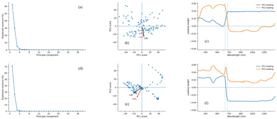
Figure 2. Canopy hyperspectral PCA for 2021 (a–c) and 2020 (d–f): explained variance (a,d), PC scores with LAI/LNA directions (b,e), and PC loading spectra (c,f).

Table 3 demonstrates that the Estimating model for LAI exhibits high fitting accuracy and consistent training-to-test performance in both 2021 and 2020, with stable test set performance indicating strong generalization capabilities. Table 4 shows that the Estimating model for LNA also achieves good prediction levels, but its inter-year error variation is more pronounced, exhibiting lower stability than LAI. The results demonstrate that the PCA–Ridge model exhibits greater stability and reliability in small-sample scenarios.

Table 3. The results of the spectral model for predicting the LAI.

Year	Dataset	n	R2	RMSE	RPD
2021	Training	78	0.95 ± 0.01 1	0.35 ± 0.04	4.73 ± 0.68
	Test	24	0.86 ± 0.06 1	0.53 ± 0.12	3.26 ± 0.75
2020	Training	73	0.94 ± 0.01 1	0.21 ± 0.03	4.21 ± 0.60
	Test	25	0.90 ± 0.04 1	0.26 ± 0.05	3.47 ± 0.66

¹ Represents p < 0.01.

Table 4. The results of the spectral model for predicting the LNA.

Year	Dataset	n	R2	RMSE (kg/ha)	RPD
2021	Training	78	0.93 ± 0.02 1	7.58 ± 0.96	3.79 ± 0.53
	Test	24	0.88 ± 0.05 1	9.56 ± 2.07	3.09 ± 0.68
2020	Training	73	0.95 ± 0.01 1	1.68 ± 0.24	4.85 ± 0.73
	Test	25	0.90 ± 0.05 1	2.36 ± 0.49	3.52 ± 0.89

¹ Represents p < 0.01.

3.2. The LAI and LNA Simulation with Remote Sensing Data Assimilation

The LAI and LNA derived from hyperspectral estimation were set as state variables in the DSSAT model simulation process. The DSSAT model was optimized using the PSO algorithm to simulate soybean LAI. The results demonstrated that employing both the LAI and LNA (V_LAI+LNA) as state variables consistently achieved optimal and reliable LAI simulation performance. The comparison between scatter points and the 1:1 line (Figure 3) indicates that when using V_LAI and V_LAI+LNA, simulated LAI values generally align well with observed measurements, with samples predominantly clustered near the 1:1 line. In contrast, the V_LNA approach exhibits more pronounced deviations (primarily overestimations) and increased dispersion in the medium-to-high LAI range, indicating that treating LNA as the sole state variable imposes relatively weak constraints on LAI. Quantitative analysis (Table 5) indicated that all simulation methods achieved a high accuracy standard, with R² exceeding 0.82 and d never falling below 0.95. For both 2021 and 2020 soybean varieties, the method using LAI and LNA (V_LAI+LNA) as state variables performed very well. In 2021, V_LAI+LNA achieved the highest explanatory power (R² = 0.93) and excellent consistency (d = 0.98). This result was comparable to using only LAI (V_LAI) (R² = 0.93, d = 0.98) and demonstrated low error (RMSE = 0.46). In 2020, V_LAI+LNA also produced strong results (R² = 0.85, d = 0.96, RMSE = 0.37), closely matching V_LAI (R² = 0.87, RMSE = 0.35). While V_LAI had a lower RMSE in 2020, V_LAI+LNA demonstrated more balanced performance across both years, with no significant drop in any key metric. V_LAI+LNA consistently outperformed the V_LNA method across all evaluation metrics for both years (R² = 0.90 and 0.82, RMSE = 0.74 and 0.40, d = 0.96 and 0.95). Thus, the combined LAI and LNA method (V_LAI+LNA) can simulate LAI reliably, performing as well as the univariate models (V_LAI/V_LNA) and possibly offering better stability.

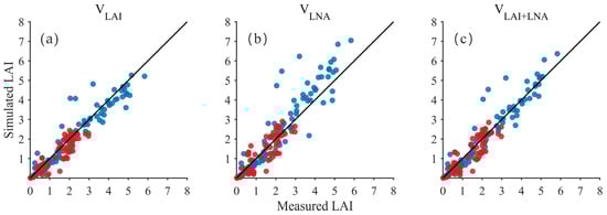
Figure 3. Relationship between simulated and measured LAI values (Black line: 1:1 Line; Blue dots: 2021 year; Red dots: 2020 year) for: (a) LAI as the state variable (V_LAI); (b) LNA as the state variable (V_LNA); (c) both LAI and LNA as state variables (V_LAI+LNA).

Table 5. The relationships between the simulated and measured LAI values.

Methods	Year	n	R2	RMSE	d
VLAI	2021	104	0.93 1	0.46	0.98
	2020	98	0.87 1	0.35	0.96
VLNA	2021	104	0.90 1	0.74	0.96
	2020	98	0.82 1	0.40	0.95
VLAI+LNA	2021	104	0.93 1	0.47	0.98
	2020	98	0.85 1	0.37	0.96

¹ Represents p < 0.01.

In addition, the results of the LNA simulation were compared using these three methods (V_LAI, V_LNA, and V_LAI+LNA). In the low LNA range (approximately 0–25), simulated values from all three methods generally align with observed values along the 1:1 line (Figure 4), indicating that each method effectively reproduces the fundamental trend of LNA variation. As LNA increases, the dispersion notably grows. However, the point clouds from the V_LNA method remain relatively closer to the 1:1 line and exhibit smaller deviations in the medium-to-high value range, suggesting that the V_LNA method enhances consistency in the high-value segment. The visual trend was confirmed by quantitative metrics in Table 6, which summarizes the validation statistics for simulating LNA using three methods (V_LAI, V_LNA, and V_LAI+LNA) across two soybean varieties in 2020 and 2021. The results indicate that the simultaneous use of LAI and LNA as state variables (V_LAI+LNA) is a viable approach for estimating LNA. Although the V_LNA method using only LNA as the state variable achieved the highest accuracy in both years (R² = 0.96 and 0.76, RMSE = 7.26 kg/ha and 5.53 kg/ha), the approach using both LAI and LNA as state variables (V_LAI+LNA) also performed well, significantly outperforming the method using only LAI as a state variable (V_LAI). Crucially, the simulated values from the V_LAI+LNA method show high consistency with observed values, as evidenced by the sustained high R² values (0.95 in 2021 and 0.72 in 2020) and consistency index d (0.97 in 2021 and 0.90 in 2020). Meanwhile, the RMSE of the V_LAI+LNA method (8.59 kg/ha in 2021 and 5.65 kg/ha in 2020) remained at a low level, showing only a slight difference compared to the V_LNA method. In summary, the method of simultaneously treating LAI and LNA as state variables (V_LAI+LNA) provides a reliable, accurate, and operationally feasible strategy for estimating LNA.

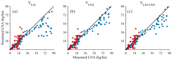
Figure 4. Relationship between simulated and measured LNA values (Black line: 1:1 Line; Blue dots: 2021 year; Red dots: 2020 year) for: (a) LAI as the state variable (V_LAI); (b) LNA as the state variable (V_LNA); (c) both LAI and LNA as state variables (V_LAI+LNA).

Table 6. The relationships between the simulated and measured values of LNA.

Methods	Year	n	R2	RMSE (kg/ha)	d
VLAI	2021	104	0.84 1	14.38	0.91
	2020	98	0.67 1	6.45	0.87
VLNA	2021	104	0.96 1	7.26	0.98
	2020	98	0.76 1	5.53	0.91
VLAI+LNA	2021	104	0.95 1	8.59	0.97
	2020	98	0.72 1	5.65	0.90

¹ Represents p < 0.01.

3.3. The Estimation of Yield

Based on remote sensing data from the soybean growth stages in 2020 and 2021, the DSSAT-CROPGRO-Soybean model was optimized to achieve effective simulation of soybean yield. Figure 5 displays the scatter plot relationship between simulated and measured yields under three methods (V_LAI, V_LNA+LNA). Compared to univariate methods, the scatter points for the V_LAI+LNA method are more concentrated near the 1:1 line with smaller deviations, indicating that the V_LAI+LNA method achieved higher consistency and lower dispersion across the two-year sample. Table 7 presents the yield outcomes obtained from simulations using three distinct state variable methods (V_LAI, V_LNA, and V_LAI+LNA) for the years 2020 and 2021. Overall, the method using both LAI and LNA as state variables (V_LAI+LNA) performed best over the two years. In 2021, the V_LAI+LNA method achieved satisfactory simulation results (R² = 0.89, RMSE = 127.05 kg/ha, d = 0.95). In 2020, the V_LAI+LNA method also yielded satisfactory simulation results (R² = 0.84, RMSE = 192.23 kg/ha, d = 0.86). In contrast, the performance of the V_LAI and V_LNA methods varied across different years. The V_LAI method yielded an R² value of 0.60 in 2020 and 0.51 in 2021, with RMSE ranging from 211.08 to 257.66 kg/ha. The V_LNA method performed notably well in 2020 (R² = 0.85, RMSE = 206.60 kg/ha) but declined in 2021 (R² = 0.55, RMSE = 281.37 kg/ha). The results indicate that the V_LAI+LNA approach yields simulation values closer to observational data and demonstrates higher overall consistency compared to the V_LAI and V_LNA methods.

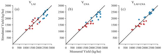
Figure 5. Relationship between simulated and measured yield values (Black line: 1:1 Line; Blue dots: 2021 year; Red dots: 2020 year) for: (a) LAI as the state variable (V_LAI); (b) LNA as the state variable (V_LNA); (c) both LAI and LNA as state variables (V_LAI+LNA).

Table 7. The relationships between the simulated and measured values of yield.

Methods	Year	n	R2	RMSE (kg/ha)	d
VLAI	2021	13	0.51 1	257.66	0.82
	2020	14	0.60 1	211.08	0.87
VLNA	2021	13	0.55 1	281.37	0.78
	2020	14	0.85 1	206.60	0.83
VLAI+LNA	2021	13	0.89 1	127.05	0.95
	2020	14	0.84 1	192.23	0.86

¹ Represents p < 0.01.

3.4. Yield Simulation Using RRMSE as the Optimization Function

In this study, the relative root mean square error (RRMSE) was also employed as an optimization function to simulate soybean yield [34]. As shown in Table 8, the simulated yields and measured yields were compared for different optimization function methods (NSE and RRMSE). When optimized using the NSE function (Table 7), the V_LAI+LNA method achieved a high goodness-of-fit (R² = 0.89 in 2021) and low error (RMSE = 127.05 kg/ha in 2021), demonstrating good consistency (d = 0.95). When using RRMSE as the optimization function (Table 8), it also demonstrated robust performance, particularly in 2021 (R² = 0.77, RMSE = 177.74 kg/ha, d = 0.92). However, the performance of the V_LAI and V_LNA methods varied across different years and optimization functions. When NSE is the objective function, the V_LNA method performed well in 2020 (R² = 0.85) but poorly in 2021 (R² = 0.55); under RRMSE optimization, the V_LNA method showed moderate performance in 2020 (R² = 0.75) but poor performance in 2021 (R² = 0.63). Furthermore, a comparison of these two optimization functions indicates that simulations using NSE as the optimization function for the V_LAI+LNA method typically yielded higher R² values and lower RMSE values than those using RRMSE as the optimization function. However, the RRMSE-based approach still produced reliable results, suggesting that employing NSE as the optimization function is feasible for soybean yield simulations.

Table 8. The production simulation results are using RRMSE as the optimization function.

Methods	Year	n	R2	RMSE (kg/ha)	d
VLAI	2021	13	0.75 1	238.60	0.86
	2020	14	0.54 1	245.52	0.83
VLNA	2021	13	0.63 1	253.08	0.83
	2020	14	0.75 1	194.09	0.85
VLAI+LNA	2021	13	0.77 1	177.74	0.92
	2020	14	0.50 1	229.00	0.83

¹ Represents p < 0.01.

4. Discussion

In the studies employing spectral inversion to estimate soybean LAI and LNA, hyperspectral data offer distinct advantages. Their continuous narrow spectral bands enable more precise characterization of leaf and canopy absorption and scattering properties, alongside spectral responses associated with components such as pigments, proteins, and nitrogen. This provides a more comprehensive information foundation for the quantitative estimation of LAI and LNA [35,36]. Existing research and reviews also indicate that LAI and LNA often exhibit heightened sensitivity in the visible-red edge-near-infrared region, with red edge information proving particularly crucial for the combined characterization of structural and pigmentary signals [37]. Unlike approaches relying on a limited number of spectral bands to construct vegetation indices, this study directly employs the full spectral range of reflectance from 350–1339 nm as input for modeling. Given the characteristics of hyperspectral data, including high dimensionality, information redundancy, and strong band-to-band correlations, direct modeling risks instability and overfitting. Consequently, dimensionality reduction and feature extraction are required to compress redundant information and enhance model robustness [38]. In the studies concerning crop trait inversion, feature compression based on methods such as PCA, combined with regularized regression employing L2 penalties (such as ridge regression and its extended forms) to stabilize estimates and enhance generalization capability, constitutes a common and effective technical approach [39]. Therefore, in estimating LAI and LNA within this study, while fully utilizing full-spectral hyperspectral information, dimensionality reduction and regularization effectively mitigate instability arising from high-dimensional strong correlations. This enables the model to maintain robust stability and predictive capability even under conditions of small sample sizes and strongly correlated spectral bands.

For the LAI simulation, the approach using both the LAI and LNA as state variables (V_LAI+LNA) achieved comparable accuracy to using the LAI alone (V_LAI), but significantly outperformed the method using only LNA as the state variable (V_LNA). This finding indicates that within the DSSAT model framework, the LAI itself serves as the most direct and sensitive state variable for simulation. Previous research has similarly demonstrated that assimilating LAI observations alone can provide the most effective constraint for model optimization [23]. For LNA simulation, the results from using both the LAI and LNA as state variables (V_LAI+LNA), while not achieving the optimal accuracy of using LNA alone (V_LNA), were significantly superior to those using only the LAI (V_LAI). This indicates that LNA is a more deeply embedded biochemical state variable driven by multiple factors. When only the LAI was used as the state variable (V_LAI), the model failed to accurately capture LNA dynamics due to the absence of direct nitrogen constraints, resulting in it achieving the poorest accuracy. For yield simulation, the method simultaneously employing the LAI and LNA as state variables (V_LAI+LNA) achieved the best performance, as it concurrently constrained two core physiological dimensions governing yield potential. When only the LAI was used as the state variable (V_LAI), the model effectively simulated canopy light interception and biomass accumulation processes; however, it failed to accurately represent the photosynthetic efficiency governed by leaf nitrogen status [40]. Conversely, when only LNA was used as the state variable (V_LNA), it could precisely characterize plant nitrogen dynamics but lacked direct constraints on canopy structural size, which could easily lead to deviations in estimating the photosynthetic “source” capacity [41,42]. The simultaneous use of the LAI and LNA (V_LAI+LNA) as state variables operated through a multi-variable coordination mechanism. This approach forced the model to optimize within a solution space concurrently satisfying observed canopy structure and nitrogen accumulation status, thereby achieving a more complete representation of photosynthetic product accumulation and these products’ partitioning to grains. In summary, the principal advantage of simultaneously using the LAI and LNA (V_LAI+LNA) as state variables lies not necessarily in achieving the absolute highest accuracy on every single metric, but rather in its exceptional robustness and well-balanced overall performance. Simulating LAI and LNA concurrently as state variables yields favorable results, reflecting the systemic optimization of multiple interdependent processes within the model, including photosynthetic production, allocation strategies, and developmental progression. This demonstrates that integrating a “structure-function” observational approach can guide crop models towards simulations that adhere to more physiologically plausible mechanisms. In summary, the core advantage of simultaneously employing LAI and LNA as state variables (V_LAI+LNA) lies not in achieving the absolute highest precision across all metrics, but in its overall performance.

This study employed two soybean varieties with distinct growth habits from 2021 and 2020 (sub-limited pod-setting habit and limited pod-setting habit), aiming to test the applicability of different state variable methods under varying management regimes and genetic backgrounds. Results indicate that concurrent application of LAI and LNA as state variable methods effectively enhances yield prediction accuracy across diverse environments and soybean varieties (Figure 5). However, the extent of correction varies between cultivars (Table 7), consistent with prior observations in soybean of “assimilation efficiency varying with spatial/management conditions, with both positive and negative assimilation efficiencies coexisting” [43]. From a physiological perspective, soybean growth habits alter canopy structure and light interception processes, thereby modifying the optimal range of LAI and its relationship with LNA. This may further influence the response relationship with yield [44]; therefore, when both LAI and LNA are employed as state variables, the sensitivity of model state updates to LAI and LNA observations, along with the correctable space, may vary across crop varieties [45,46]. Moreover, key physiological processes within crop models are frequently characterized by variety-specific genetic coefficients/genotype-specific parameters, which exhibit significant genetic variation and are closely correlated with the formation of phenotypes [25,47]. Against this backdrop, when constraining model parameters and states using remotely sensed LAI and LNA, varietal differences may alter the discernibility of observation operators and the compensatory relationships between parameters and states. This, in turn, may result in varying assimilation efficiencies across different varieties [45,48]. However, the optimization function of the PSO algorithm employed in this study did not analyze the weight allocation issue arising from interactions between LAI and LNA. Consequently, future research should examine the impact of different weighting variables on yield simulation when multiple state variables are involved, thereby clarifying the applicability and optimization direction of various state variables under different genetic backgrounds.

In the DSSAT model, calibrating genotype-specific parameters is critical for accurate yield simulation. Consequently, selecting an appropriate optimization objective is equally crucial for the success of any optimization algorithm. This study demonstrated the feasibility of selecting the NSE coefficient as the objective function for the PSO algorithm. The primary rationale is that using the NSE as the objective function not only reduces the absolute error in simulated yield but also, due to its robustness, mitigates the interference from observation noise. More importantly, it effectively captures the dynamic processes and trends of yield formation, thereby ensuring close alignment between the simulated results and observations for both the developmental trajectory and the outcome [23,24]. While this study has validated the feasibility and effectiveness of the proposed method, the algorithmic performance remains subject to the influence of problem-specific configurations [49]. Furthermore, for the process-based DSSAT model, potential parameter interactions may complicate the optimization landscape. A promising direction for future research is to establish multi-objective optimization frameworks that concurrently address yield, physiological processes, and phenological development, thereby advancing the calibration methodology towards greater efficiency and robustness. However, this study demonstrated the potential of this approach for both mechanistic research and yield estimation by utilizing hyperspectral data to simultaneously simulate yield using LAI and LNA as state variables at both the field scale and in pot experiments. Hyperspectral data possess inherent advantages for deriving biogeochemical parameters such as LAI and LNA due to their continuous, narrow spectral bands. Nevertheless, the considerable time costs associated with data acquisition and processing, coupled with the uncertainty inherent in inversion results, directly impact assimilation systems. Consequently, this limits the scalability of hyperspectral data across spatial and temporal scales. When extending multispectral data to regional scales, although its accuracy in deriving biogeochemical parameters falls short of hyperspectral data, it offers the advantages of extensive coverage and repeat observations. However, variations in soil, climate, and management practices across the region impose greater demands on crop model parameter optimization and assimilation strategies. Concurrently, the optimization algorithms employed in this study necessitate extensive iterative model runs. When extending hyperspectral data applications to regional scales, computational efficiency will become a limiting factor constraining their broader implementation.

It should be noted that this study focuses on verifying the feasibility of jointly optimizing soybean LAI, LNA, and yield using NSE as the objective function, and does not conduct a systematic statistical assessment of the random variability inherent in PSO (such as the mean and variance across multiple independent runs). To ensure reproducibility of results, this study executed the PSO algorithm only once under fixed random seed conditions; existing comparative studies of PSO variants also employed fixed random seeds and reported results from a single run [50]. Research on automatic calibration of crop models indicates that under identical data and algorithm settings, optimal parameters obtained from repeated runs often exhibit insignificant variation. Furthermore, when convergence behavior stabilizes, the marginal benefit of repeated runs becomes limited [51]. Meanwhile, process-driven model calibration typically requires numerous model invocations and incurs high computational overhead [52,53]; this study did not conduct multiple independent repeated runs. Based on the above considerations, this study compared two soybean materials with different growth habits from 2020 and 2021: Results indicate that using NSE as the optimization function yields superior overall performance in simulating LAI, LNA, and yield; using RRMSE as the optimization function also yielded satisfactory yield simulations, though its composite metrics were slightly inferior to NSE. Furthermore, both optimization functions exhibited excellent convergence curves (Figure S1). The aforementioned multi-instance validation and convergence behavior collectively support that, under the research objective of “optimization function feasibility and comparison” in this study, a single PSO optimization execution can provide reliable parameter estimation results. Future research will further evaluate the stability and results credibility of PSO through multiple independent runs and uncertainty quantification (e.g., distribution of repeated runs/confidence intervals) in a more systematic manner.

5. Conclusions

Based on field and pot experiments, the leaf area index (LAI) and leaf nitrogen accumulation (LNA) were estimated using the canopy spectral data of soybeans. These estimates were employed as state variables in three crop growth modeling approaches, with the NSE serving as the objective function during optimization to simulate soybean yield. The three approaches involved (i) using only the LAI as the state variable (V_LAI), (ii) using only LNA as the state variable (V_LNA), and (iii) simultaneously using both the LAI and LNA as state variables (V_LAI+LNA). The findings revealed that the method of simultaneously using LAI and LNA as state variables (V_LAI+LNA) demonstrates its stability and feasibility in estimating the LAI and LNA of soybeans, and shows more outstanding effects in terms of yield. Synergistically regulating the leaf area index and leaf nitrogen accumulation enabled the crop growth model to simulate the crop growth process more realistically. Furthermore, employing the NSE as the objective function effectively captured the dynamic processes and trends of yield formation, demonstrating the feasibility of optimizing state variables in crop growth models. Therefore, this study provides a robust methodology for estimating soybean yield by integrating remote sensing data with crop growth models. This methodology can be applied to other crops. This study validated the effectiveness of the synergistic assimilation framework at the field scale; however, its application remains constrained by the reliance on hyperspectral data, challenges in regional-scale extension, and uncertainties inherent in the assimilation process. Future research should focus on developing operational solutions based on multispectral data, constructing computationally efficient regional assimilation systems, and thoroughly quantifying uncertainties to advance this methodology from mechanism validation towards widespread application.

References

- Crusiol, L.G.T.; Sun, L.; Sibaldelli, R.N.R.; Felipe, J.V.; Furlaneti, W.X.; Chen, R.; Sun, Z.; Wu, Y.D.; Chen, Z.; Nanni, M.R.; et al. Strategies for monitoring within-field soybean yield using Sentinel-2 Vis-NIR-SWIR spectral bands and machine learning regression methods. Precis. Agric. 2022, 23, 1093–1123. [Google Scholar] [CrossRef]
- Lu, W.; Du, R.T.; Niu, P.S.; Xing, G.N.; Luo, H.; Deng, Y.M.; Shu, L. Soybean Yield Preharvest Prediction Based on Bean Pods and Leaves Image Recognition Using Deep Learning Neural Network Combined with GRNN. Front. Plant Sci. 2022, 12, 791256. [Google Scholar] [CrossRef] [PubMed]
- Pei, J.; Zou, Y.P.; Liu, Y.B.; He, Y.N.; Tan, S.F.; Wang, T.X.; Huang, J.X. Downscaling Administrative-Level Crop Yield Statistics to 1 km Grids Using Multisource Remote Sensing Data and Ensemble Machine Learning. IEEE J. Sel. Top. Appl. Earth Obs. Remote Sens. 2024, 17, 14437–14453. [Google Scholar]
- de Freitas, R.G.; Oldoni, H.; Joaquim, L.F.; Pozzuto, J.V.F.; do Amaral, L.R. Predicting on-farm soybean yield variability using texture measures on Sentinel-2 image. Precis. Agric. 2024, 25, 2977–3000. [Google Scholar] [CrossRef]
- Joshi, A.; Pradhan, B.; Gite, S.; Chakraborty, S. Remote-Sensing Data and Deep-Learning Techniques in Crop Mapping and Yield Prediction: A Systematic Review. Remote Sens. 2023, 15, 2014. [Google Scholar]
- Najjar, H.; Miranda, M.; Nuske, M.; Roscher, R.; Dengel, A. Explainability of Subfield Level Crop Yield Prediction Using Remote Sensing. IEEE J. Sel. Top. Appl. Earth Obs. Remote. Sens. 2025, 18, 4141–4161. [Google Scholar] [CrossRef]
- Mena, F.; Pathak, D.; Najjar, H.; Sanchez, C.; Helber, P.; Bischke, B.; Habelitz, P.; Miranda, M.; Siddamsetty, J.; Nuske, M.; et al. Adaptive fusion of multi-modal remote sensing data for optimal sub-field crop yield prediction. Remote Sens. Environ. 2025, 318, 114547. [Google Scholar] [CrossRef]
- Zare, H.; Weber, T.K.; Ingwersen, J.; Nowak, W.; Gayler, S.; Streck, T. Within-season crop yield prediction by a multi-model ensemble with integrated data assimilation. Field Crop. Res. 2024, 308, 109293. [Google Scholar] [CrossRef]
- Hao, S.R.; Ryu, D.; Western, A.; Perry, E.; Bogena, H.; Franssen, H.J.H. Performance of a wheat yield prediction model and factors influencing the performance: A review and meta-analysis. Agric. Syst. 2021, 194, 103278. [Google Scholar] [CrossRef]
- Manivasagam, V.S.; Sadeh, Y.; Kaplan, G.; Bonfil, D.J.; Rozenstein, O. Studying the Feasibility of Assimilating Sentinel-2 and PlanetScope Imagery into the SAFY Crop Model to Predict Within-Field Wheat Yield. Remote Sens. 2021, 13, 2395. [Google Scholar] [CrossRef]
- Chen, Y.B.; Wang, S.Y.; Xue, Z.K.; Hu, J.J.; Chen, S.J.; Lv, Z.F. Rice Growth Estimation and Yield Prediction by Combining the DSSAT Model and Remote Sensing Data Using the Monte Carlo Markov Chain Technique. Plants 2025, 14, 1206. [Google Scholar] [CrossRef]
- Han, D.C.; Wang, P.J.; Tang, J.X.; Li, Y.; Wang, Q.; Ma, Y.P. Enhancing crop yield forecasting performance through integration of process-based crop model and remote sensing data assimilation techniques. Agric. For. Meteorol. 2025, 372, 110696. [Google Scholar] [CrossRef]
- Rinaldi, M.; Satalino, G.; Mattia, F.; Balenzano, A.; Perego, A.; Acutis, M.; Ruggieri, S. Assimilation of COSMO-SkyMed-derived LAI maps into the AQUATER crop growth simulation model. Capitanata (Southern Italy) case study. Eur. J. Remote Sens. 2013, 46, 891–908. [Google Scholar]
- Jiang, Z.; Chen, Z.; Chen, J.; Ren, J.; Li, Z.; Sun, L. The estimation of regional crop yield using ensemble-based four-dimensional variational data assimilation. Remote Sens. 2014, 6, 2664–2681. [Google Scholar] [CrossRef]
- Thorp, K.R.; Wang, G.; West, A.L.; Moran, M.S.; Bronson, K.F.; White, J.W.; Mon, J. Estimating crop biophysical properties from remote sensing data by inverting linked radiative transfer and ecophysiological models. Remote Sens. Environ. 2012, 124, 224–233. [Google Scholar] [CrossRef]
- Jin, X.; Li, Z.; Feng, H.; Ren, Z.; Li, S. Estimation of maize yield by assimilating biomass and canopy cover derived from hyperspectral data into the AquaCrop model. Agric. Water Manag. 2020, 227, 105846. [Google Scholar] [CrossRef]
- Li, Z.; Wang, J.; Xu, X.; Zhao, C.; Jin, X.; Yang, G.; Feng, H. Assimilation of two variables derived from hyperspectral data into the DSSAT-CERES model for grain yield and quality estimation. Remote Sens. 2015, 7, 12400–12418. [Google Scholar]
- Liu, D.D. Hypothesis Testing for the Difference between Two Nash-Sutcliffe Efficiencies for Comparing Hydrological Model Performance. J. Hydrol. Eng. 2024, 29, 04024015. [Google Scholar] [CrossRef]
- Shen, Y.; Li, H.M.; Zhang, B.; Cao, Y.; Guo, Z.W.; Gao, X.; Chen, Y.P. An artificial neural network-based data filling approach for smart operation of digital wastewater treatment plants. Environ. Res. 2023, 224, 115549. [Google Scholar] [CrossRef]
- Price, K.; Purucker, S.T.; Kraemer, S.R.; Babendreier, J.E. Tradeoffs among watershed model calibration targets for parameter estimation. Water Resour. Res. 2012, 48, W10542. [Google Scholar] [CrossRef]
- Lee, J.S.; Choi, H.I. A rebalanced performance criterion for hydrological model calibration. J. Hydrol. 2022, 606, 127372. [Google Scholar] [CrossRef]
- Martin, D.; Katja, B.; Matthias, W.; Wolfram, M.; Tobias, H. Retrieval of Biophysical Crop Variables from Multi-Angular Canopy Spectroscopy. Remote Sens. 2017, 9, 726. [Google Scholar]
- Mridha, N.; Sahoo, R.N.; Sehgal, V.K.; Krishna, G.; Pargal, S.; Pradhan, S.; Gupta, V.K.; Kumar, D.N. Comparative evaluation of inversion approaches of the radiative transfer model for estimation of crop biophysical parameters. Int. Agrophys. 2015, 29, 201–212. [Google Scholar] [CrossRef]
- Matthias, L.; Tobias, H.; Martin, D.; Wolfram, M. Retrieval of Seasonal Leaf Area Index from Simulated EnMAP Data through Optimized LUT-Based Inversion of the PROSAIL Model. Remote Sens. 2015, 7, 10321–10346. [Google Scholar]
- Boote, K.J.; Jones, J.W.; Batchelor, W.D.; Nafziger, E.D.; Myers, O. Genetic coefficients in the CROPGRO–Soybean Model: Links to field performance and genomics. Agron. J. 2003, 95, 32–51. [Google Scholar]
- Jolliffe, I.T. Principal Component Analysis, 2nd ed.; Springer: New York, NY, USA, 2002. [Google Scholar]
- Næs, T.; Martens, H. Principal Component Regression in NIR Analysis: Viewpoints, Background Details and Selection of Components. J. Chemom. 1988, 2, 155–167. [Google Scholar] [CrossRef]
- Hoerl, A.E.; Kennard, R.W. Ridge Regression: Biased Estimation for Nonorthogonal Problems. Technometrics 1970, 12, 55–67. [Google Scholar] [CrossRef]
- Hastie, T.; Tibshirani, R.; Friedman, J. The Elements of Statistical Learning: Data Mining, Inference, and Prediction, 2nd ed.; Springer: New York, NY, USA, 2009. [Google Scholar]
- Vigneau, E.; Devaux, M.-F.; Qannari, E.M.; Robert, P. Principal Component Regression, Ridge Regression and Ridge Principal Componen Regression in Spectroscopy Calibration. J. Chemom. 1997, 11, 239–249. [Google Scholar] [CrossRef]
- Eberhart, R.; Kennedy, J. A New optimizer using particle swarm theory. In Proceedings of the MHS’95, the Sixth International Symposium on Micro Machine and Human Science, Nagoya, Japan, 4–6 October 1995; pp. 39–43. [Google Scholar]
- Clerc, M. Standard Particle Swarm Optimisation (SPSO-2011). 2011. Available online: http://clerc.maurice.free.fr/pso/SPSO_descriptions.pdf (accessed on 26 January 2026).
- Zhang, Y.; Zhang, Y.; Jiang, H.; Tang, L.; Liu, X.; Cao, W.; Zhu, Y. Effects of different observed datasets on the calibration of crop model parameters with GLUE: A case study using the CROPGRO-Soybean phenological model. PLoS ONE 2024, 19, e0302098. [Google Scholar] [CrossRef]
- Zhu, B.; Chen, S.; Xu, Z.; Ye, Y.; Han, C.; Lu, P.; Song, K. The Estimation of Maize Grain Protein Content and Yield by Assimilating LAI and LNA, Retrieved from Canopy Remote Sensing Data, into the DSSAT Model. Remote Sens. 2023, 15, 2576. [Google Scholar] [CrossRef]
- Burnett, A.C.; Anderson, J.; Davidson, K.J.; Ely, K.S.; Lamour, J.; Li, Q.; Morrison, B.D.; Yang, D.; Rogers, A.; Serbin, S.P. A best-practice guide to predicting plant traits from leaf-level hyperspectral data using partial least squares regression. J. Exp. Bot. 2021, 72, 6175–6189. [Google Scholar] [CrossRef] [PubMed]
- Wang, D.; Struik, P.C.; Liang, L.; Yin, X. Estimating leaf and canopy nitrogen contents in major field crops across the growing season from hyperspectral images using nonparametric regression. Comput. Electron. Agric. 2025, 233, 110147. [Google Scholar] [CrossRef]
- Yan, K.; Gao, S.; Yan, G.; Ma, X.; Chen, X.; Zhu, P.; Li, J.; Gao, S.; Gastellu-Etchegorry, J.-P.; Myneni, R.B.; et al. A global systematic review of the remote sensing vegetation indices. Int. J. Appl. Earth Obs. Geoinf. 2025, 139, 104560. [Google Scholar]
- Cao, C.; Wang, T.; Gao, M.; Li, Y.; Li, D.; Zhang, H. Hyperspectral inversion of nitrogen content in maize leaves based on different dimensionality reduction algorithms. Comput. Electron. Agric. 2021, 190, 106461. [Google Scholar] [CrossRef]
- Singh, P.; Srivastava, P.K.; Jha, P.K.; Verrelst, J.; Singh, P.N.; Prasad, R. Retrieval of crop traits using PROSAIL-based hybrid radiative transfer model and EnMAP hyperspectral data. Int. J. Appl. Earth Obs. Geoinf. 2025, 143, 104769. [Google Scholar] [CrossRef]
- Tang, Z.J.; Wang, X.; Xiang, Y.Z.; Liang, J.P.; Guo, J.J.; Li, W.Y.; Lu, J.S.; Du, R.Q.; Li, Z.J.; Zhang, F.C. Application of hyperspectral technology for leaf function monitoring and nitrogen nutrient diagnosis in soybean (Glycine max L.) production systems on the Loess Plateau of China. Eur. J. Agron. 2024, 154, 127098. [Google Scholar] [CrossRef]
- Wang, J.; Chen, S.T.; Ding, S.C.; Yao, X.W.; Zhang, M.M.; Hu, Z.H. Relationships Between the Leaf Respiration of Soybean and Vegetation Indexes and Leaf Characteristics. Spectrosc. Spectr. Anal. 2022, 42, 1607–1613. [Google Scholar]
- Fan, Z.; Qiang, B.B.; Zhang, X.B.; Lin, Y.R.; Wu, Y.L.; Zhao, X.N.; Liu, E.K.; Cai, T.; Zhang, P.; Liu, T.N.; et al. Optimizing light and nitrogen distribution in maize-soybean intercropping systems to enhance crop yield. Eur. J. Agron. 2026, 172, 127853. [Google Scholar] [CrossRef]
- Gaso, D.V.; de Wit, A.; de Bruin, S.; Puntel, L.A.; Berger, A.G.; Kooistra, L. Efficiency of assimilating leaf area index into a soybean model to assess within-field yield variability. Eur. J. Agron. 2023, 143, 126718. [Google Scholar] [CrossRef]
- Tagliapietra, E.L.; Streck, N.A.; da Rocha, T.S.M.; Richter, G.L.; da Silva, M.R.; Cera, J.C.; Guedes, J.V.C.; Zanon, A.J. Optimum leaf area index to reach soybean yield potential in subtropical environment. Agron. J. 2018, 110, 932–938. [Google Scholar] [CrossRef]
- Huang, J.; Gómez-Dans, J.L.; Huang, H.; Ma, H.; Wu, Q.; Lewis, P.E.; Liang, S.; Chen, Z.; Xue, J.-H.; Wu, Y.; et al. Assimilation of remote sensing into crop growth models: Current status and perspectives. Agric. For. Meteorol. 2019, 276–277, 107609. [Google Scholar] [CrossRef]
- Jin, X.; Kumar, L.; Li, Z.; Feng, H.; Xu, X.; Yang, G.; Wang, J. A review of data assimilation of remote sensing and crop models. Eur. J. Agron. 2018, 92, 141–152. [Google Scholar] [CrossRef]
- Yan, W.; Jiang, H.; Xu, J.; Li, T.; Begum, N.; Karikari, B.; Liu, L.; Zhao, T. Genetic analysis of genotype-specific parameters in the DSSAT-CROPGRO-soybean phenology simulation model via a multi-GWAS method. Field Crop. Res. 2023, 304, 109165. [Google Scholar]
- Richetti, J.; Cohan, S.H.; Temps, J.P.; Borges, P.; Marin, F.R. Remotely sensed vegetation index and LAI-derived parameter determination for the CSM-CROPGRO-Soybean model. Int. J. Appl. Earth Obs. 2019, 79, 110–115. [Google Scholar]
- Bettina, S.; Hoshin, V.G. Do Nash values have value? Hydrol. Process. 2007, 21, 2075–2080. [Google Scholar] [CrossRef]
- Liu, Y.; Shi, X.; Meng, S.; Yang, W.; Fang, Z.; Cai, Z.; Li, H. Adaptive hierarchical filtering particle swarm optimization for multiple magnetic dipoles modeling of space equipment. Sci. Rep. 2025, 15, 33946. [Google Scholar] [CrossRef]
- Zhang, Y.; Zhang, Y.; Jiang, H.; Tang, L.; Liu, X.; Cao, W.; Zhu, Y. Comparison of three algorithms for estimating crop model parameters based on multi-source data: A case study using the CROPGRO-Soybean phenological model. PLoS ONE 2025, 20, e0323927. [Google Scholar]
- Tsai, W.-P.; Feng, D.; Pan, M.; Beck, H.; Lawson, K.; Yang, Y.; Liu, J.; Shen, C. From calibration to parameter learning: Harnessing the scaling effects of big data in geoscientific modeling. Nat. Commun. 2021, 12, 5988. [Google Scholar] [CrossRef]
- Johnston, D.B.; Pembleton, K.G.; Huth, N.I.; Deo, R.C. Comparison of machine learning methods emulating process driven crop models. Environ. Model. Softw. 2023, 162, 105634. [Google Scholar] [CrossRef]
Disclaimer/Publisher’s Note: The statements, opinions and data contained in all publications are solely those of the individual author(s) and contributor(s) and not of MDPI and/or the editor(s). MDPI and/or the editor(s) disclaim responsibility for any injury to people or property resulting from any ideas, methods, instructions or products referred to in the content. |
© 2026 by the authors. Licensee MDPI, Basel, Switzerland. This article is an open access article distributed under the terms and conditions of the Creative Commons Attribution (CC BY) license.