Highlights
What are the main findings?
- This study evaluates the temporal variability and algorithm differences in soil moisture estimates over Europe using ECMWF and SMAP products.
- The innovation of the study lies within the detailed analyses of impacts of hydrometeorological conditions on product performance at seasonal and short-term time-scales.
What are the implications of the main findings?
- This study found an overestimation of the magnitude of absolute soil moisture variability within both products at most stations due to an overestimation of short-term fluctuations.
- The magnitude of temporal variability and accuracy in soil moisture products depend on site-specific characteristics and the pre-processing of the data.
Abstract
This study evaluates temporal variability and algorithm differences in soil moisture estimates over Europe using the European Center for Medium-range Weather Forecasts (ECMWF) operational analysis and the passive Soil Moisture Active Passive (SMAP) soil moisture product. While models and satellite retrievals have improved in capturing the timing of soil moisture dynamics, absolute accuracy and temporal variability magnitudes still diverge. This study compares the representation of short-term and seasonal variability of soil moisture in absolute and normalized terms over two different hydrometeorological growing periods (2021 and 2022). Both datasets exhibit intermediate to high temporal correlations with in situ measurements at selected stations (median Pearson correlation coefficients of all stations range between 0.65 and 0.79), confirming previous studies. However, they overestimate the magnitude of absolute soil moisture variability at most stations (median interquartile range of all stations at 0.085 (0.10) m3m−3 for ECMWF and 0.072 (0.079) m3m−3 for SMAP opposed to 0.063 (0.072) m3m−3 for in situ in 2021 (2022)) due to an overestimation of short-term fluctuations, especially at dry stations in southern France and Eastern Europe. The soil wetness index is underestimated, particularly within SMAP estimates. The performance of both is sensitive to hydrometeorological conditions, with the 2022 European drought causing strong seasonal and weak short-term fluctuations. This is easier to capture than conditions with pronounced short-term and weaker seasonal fluctuations, as in 2021. Overall, SMAP and ECMWF time series show considerable coincident timing, whereas the magnitude of temporal variability and accuracy depend on site-specific characteristics and the pre-processing of the data.
1. Introduction
Soil moisture has been identified as a key component of the Earth system and is, therefore, recognized as an essential climate variable (ECV) [1]. Understanding the spatiotemporal dynamics of soil moisture is crucial in the context of climate change and meteorological as well as hydrological extremes because water availability influences droughts [2], wildfires [3], land–climate interactions [4,5], soil drying [6], plant water uptake processes [7], and the length and intensity of different environmental processes, such as heatwaves [8,9,10]. Further, forecasts of soil moisture dynamics are highly relevant for climate modeling, including hydrology, meteorology, ecology, agriculture, and water management on scales ranging from field to continental and even global scales [1,11,12], and a range of applications across Earth system studies (e.g., wildfire risk assessment, crop yields, forest decline). A big challenge for these applications is the requirement for spatially resolved data, which captures the temporal dynamics under different spatially distributed hydrometeorological conditions for a variety of ecosystems. As an example, sub-seasonal to seasonal forecasts and climate projections gain forecast strength by accurately initializing soil moisture and other surface fields [13]. In short-term forecasts, not only do surface flux calculations respond to different initial soil moisture conditions, but planetary boundary layer evolution and downstream environmental conditions do as well [14]. Additionally, the spatial distribution of soil moisture is a crucial factor for capturing the location of convective precipitation events, which contribute between 20% and 50% of the precipitation in summer over Europe [15], as it co-determines the location of updrafts over dry patches [16]. Precipitation events, in turn, together with the local soil types, impact the spatiotemporal dynamics of soil moisture.
Over the past decades, two approaches for the derivation of spatially resolved soil moisture fields have been used to generate a variety of soil moisture products. Firstly, there is the deterministic model-based approach with and without assimilating observational data [17]. The former is known as analysis and reanalysis data, and the latter is known as data from open-loop models to produce transient model simulations. Secondly, there are satellite remote sensing-based datasets derived from either single sensors or multi-sensor merged satellite products [17]. Models commonly simulate soil moisture by integrating differential equations that consider inflows (precipitation and infiltration) and outflows (root water uptake, bare soil evaporation, runoff, and percolation) of water in multiple discrete layers. In recent years, fully coupled models have started to be operated at progressively higher spatial resolutions. This is associated with a requirement for an increasingly detailed representation of the physical processes in the lower boundary in the model setup. The model topography, the land cover, and the soil characteristics are more realistically represented in a simulation with a finer grid. Those factors are fundamental for the simulation of soil moisture. The soil moisture content, in turn, impacts the partitioning of the heat fluxes at the land surface by potentially limiting the latent heat flux, and thus, it is one factor controlling the ratio between moisture and heat entering the overlying atmosphere (e.g., [18]).
In addition to models, satellite-based datasets can be retrieved from passive and active microwave sensors at different frequency bands [19]. Active sensors (e.g., Sentinel-1, TerraSAR-X) provide data on high spatial resolution at the expense of temporal resolution and more complex scattering effects due to, for example, surface roughness and vegetation [20]. Passive microwave radiometers have a temporal resolution of ~3 days at the equator, with one morning and one evening overpass, but they have coarse spatial resolution in the order of tens of kilometers (e.g., Soil Moisture Active Passive (SMAP), Soil Moisture Ocean Salinity (SMOS), Advanced Microwave Scanning Radiometer (AMSR2)). The most promising results for soil moisture are retrieved at the L-band (1.4 GHz) [19] due to an optimal balance between sensitivity to soil moisture, increased penetration into the vegetation, and a minimized influence from other aspects, such as surface roughness and vegetation geometry. The two missions currently retrieving soil moisture from a radiometer at the L-band are the SMOS mission launched in 2010 [21,22] and the SMAP mission launched in 2015 [23]. Apart from the sensitivity to soil moisture, the advantage of those missions is that the temporal resolution of products derived from microwave observations is not hampered by weather, sun glint, and darkness compared to optical remote sensing. The use of observations for data assimilation in model systems and the use of model-based temperature in satellite retrievals show that state-of-the-art approaches already exhibit interdependencies between remote sensing and modeling.
Estimating soil moisture using either models or remote sensing techniques is challenging due to multiple influences. A key aspect is that they must fulfill quality requirements and need appropriate validation strategies against ground truth in situ data [24]. Previous intercomparisons among and between remote sensing-based and model-based soil moisture products [17,19,25,26,27,28,29,30,31,32,33,34] show that despite considerable advancements in the algorithm architecture to improve the retrieval accuracy during recent years, there is room for reducing errors and achieving even higher accuracies [35]. Both approaches depend on a suite of assumptions required to produce a fully resolved spatial grid, and both cause uncertainties in their estimates. Of these assumptions, several factors were reported to contribute to uncertainty and errors in soil moisture retrievals and simulated products and thus produce disagreements between satellite and model-based products. This includes physical factors such as climate, vegetation density, topography [31], and soil texture [36]. Also, technical factors are relevant, like the dielectric mixing model applied [37], the choice of the algorithm [32], the temporal and spatial resolution, the measuring technique, and the frequency band used [19,29]. Despite remaining errors, the soil moisture products usually perform well in representing the timing of temporal variability, e.g., [17], which is usually due to long-term seasonal patterns. However, previous assessments generally focused on the timing of temporal soil moisture dynamics within each product (shown by the temporal correlation coefficient) and errors depicted by root mean square metrics but did usually not temporally decompose soil moisture signals in seasonal and shorter time scales. One study performed by [38] evaluated the importance of different time scales for the assimilation of soil moisture in modeling systems and showed the importance of considering the variability characteristics at different time scales.
In this study, we conduct a comprehensive assessment of similarities and differences in the temporal dynamics in terms of both the timing and the magnitude of fluctuations. All comparisons are conducted for the overall time series as well as the decomposed seasonal and short-term fluctuation signals for two (2021 and 2022) hydrometeorologically differing vegetation periods. The years 2021 and 2022 were chosen in order to be able to compare humid conditions in 2021 and severe drought conditions in 2022 across Central Europe. We will use these two vegetation period time series for comparison and for investigating the soil moisture accuracy and the representation of temporal dynamics in the chosen datasets. Spatial representativeness errors due to the scale gap are kept in mind when comparing gridded data with in situ station point measurements. We compare soil moisture temporal dynamics from the European Center for Medium-range Weather Forecasts (ECMWF) operational analysis and the SMAP DCA product at in situ measuring station networks across Europe from the Integrated Carbon Observation System (ICOS) and International Soil Moisture Network (ISMN) networks. Europe is chosen as the region of interest since it is one of the continents with the densest in situ measuring station networks besides North America and covers a large diversity in climates and eco-regimes, which makes it an ideal study region.
Thus, in this study, the work focuses on answering the following questions. (1) To what extent do ECMWF operational analysis and SMAP retrievals compare regarding their accuracy and representation of seasonal and short-term temporal dynamics at varying in situ stations across Europe? (2) In which cases and how do the prevailing hydrometeorological conditions influence their performance? (3) We also consider site characteristics (e.g., soil texture or land cover) in the interpretation of the performance of the products.
2. Materials and Methods
2.1. Data
The following sub-chapter introduces the SMAP product, the ECMWF operational analysis, and the in situ measurements with their product-specific characteristics. A summary of the spatial and temporal resolution, along with measurement depth and original units, is provided in Table 1.

Table 1.
Basic information about the datasets under investigation.
These two gridded products were chosen since they are used very frequently alongside a few other products (i.e., SMOS, Sentinel-1) and due to the similarity of their spatial resolution. The ECMWF operational analysis represents the baseline for one of the high-resolution forecast systems currently available and running at ECMWF. Considering the horizontal and vertical model resolution in combination with the usage of a sophisticated 4D-Var data assimilation scheme, ECMWF operational analysis is a representative model database. The ECMWF operational analysis can be used to initialize and force model case studies up to large-eddy simulation (LES) scale (e.g., [40,41]). For the remote sensing approach, SMAP and SMOS are the only two operational satellite remote sensing products at an L-band frequency that are currently available [42]. Different studies showed that SMAP outperforms SMOS in many regions, including Europe, e.g., [17,43]. Since SMOS is already assimilated in the ECMWF analysis product, we limited the comparison to the independent (not assimilated) SMAP dataset in this study to avoid statistical issues.
2.1.1. SMAP Satellite Remote Sensing Product
The National Aeronautics and Space Administration’s (NASA) Soil Moisture Active Passive (SMAP) mission was designed to retrieve global time series of soil moisture and freeze–thaw state over the land surfaces [23] and was launched in April 2015. The space-borne instrument is equipped with a joint L-band radar–radiometer sensor for combined active–passive microwave sensing. This setup leads to a spatial resolution of 36 km (radiometer only) and a minimum temporal resolution of 2–3 days (if not better), depending on latitude. A radar instrument failure in July 2015 meant that no further active microwave observations could be generated, while passive microwave (radiometer) observations continue to be recorded operationally since its launch. The SMAP data used in this study is the SPL3SMP_E product [44], which includes morning and afternoon satellite overpasses. Its 9 km gridding is obtained thanks to an enhanced interpolation of the coarser resolution brightness temperature scenes [45].
Here, we focus on the baseline algorithm of SMAP: Level 3-Dual Channel Algorithm (DCA; [46]). SMAP algorithms, per se, require static and dynamic ancillary data. Static ancillary data are permanent masks, e.g., for land versus water, elevation and slope, and soil properties, while dynamic ancillary data involve precipitation for quality flagging, surface roughness, and vegetation indices, like the Normalized Difference Vegetation Index (NDVI). The satellite-based NDVI product is used to constrain the joint soil moisture and vegetation optical depth retrievals [47,48,49]. Temperature and precipitation fields used in the SMAP retrieval originate from a data assimilation system. Other auxiliaries, such as soil roughness and vegetation scattering albedo, are approximated through fixed values obtained from the literature or through constant values, which are updated once a year, to keep the system of equations for the retrieval balanced and solvable. The post-processing of the SMAP soil moisture deployed here consists of filtering cells with non-optimum quality flags and surface properties and regridding the remaining data to the ECMWF grid using nearest neighborhood interpolation and eventually computing 3-day running means from the orbital fields. This practice ensures continuous, gapless, Europe-wide maps of soil moisture from the satellite remote sensing data.
2.1.2. ECMWF Operational Analysis
The Integrated Forecast System (IFS) of ECMWF is a global numerical weather prediction system. The data used in this study is based on the configuration of Cy47r3. It consists of a spectral atmospheric model with a terrain-following vertical coordinate system applied at a horizontal resolution of 0.09° and 137 vertical levels. The analysis serves as the initial condition for the high-resolution 10-day forecasts from ECMWF. The ECMWF operational analysis investigated in this study is the output of a 4D-Var data assimilation system. The system merges an earlier forecast of the model with newly approaching observations to provide 6-hourly analysis fields at 00, 06, 12, and 18 UTC daily [50]. Physical processes too small to be explicitly resolved by the model grid need to be parameterized [51]. Processes in the atmosphere relevant for computing soil moisture are parameterized in the short- and longwave radiation schemes [52], convection is parameterized by a modified version of the Tiedtke scheme [53,54], and the cloud microphysics scheme is based on [55] with several improvements implemented [56,57]. Soil moisture itself is numerically determined in the land surface scheme (HTESSEL), which uses a tiled approach representing different sub-grid surface types for vegetation, bare soil, snow, and open water. It distinguishes four soil layers, of which the first three receive input from observations via data assimilation [58,59]. The computation of soil moisture involves assimilating surface synoptic observations (SYNOP) from weather stations, like relative humidity and temperature, as well as soil moisture from the European Organisation for the Exploitation of Meteorological Satellites (EUMETSAT) Meteorological Operational satellites (MetOp-A and MetOp-B), Advanced Scatterometer (ASCAT), and NASA’s SMOS [50].
The model only determines the vertical movement of water in the unsaturated zone of the soil, while lateral movements of water between the soil columns are not considered. The top boundary condition is precipitation less evaporation and surface runoff, and the lower boundary is free drainage. The impact of the land cover on the water budget is considered with an interception reservoir, which can store a small part of the precipitation at the vegetation level. Additionally, the high and low vegetation fractions extract water from the soil via their roots and release it into the atmosphere. The integration of the equations for the calculation of soil moisture requires the specification of the hydraulic diffusivity and hydraulic conductivity of the soil, which are parameterized as functions of the soil water content and soil texture. For both soil properties, minimum values are assumed for permanent wilting point conditions, below which the soil moisture cannot drop. The land surface scheme ecLand uses the dominant soil texture class for each grid point from the FAO dataset [60]. The soil properties are tabulated for the 11 soil classes of the US Department of Agriculture soil classification. When the liquid precipitation at the surface exceeds the maximum infiltration rate or a fraction of the pixel is considered saturated, the excess water is put into direct surface runoff.
2.1.3. In Situ Observations
For comparison with SMAP and ECMWF, in situ soil moisture measurements from the ISMN ([61]; https://ismn.earth/en/ (accessed on 22 May 2024)) and ICOS ([62]; https://www.icos-cp.eu/observations/station-network (accessed on 10 March 2023)) networks were acquired across Europe. The ISMN, funded by the European Space Agency (ESA), was established as a community effort to collect and freely share global soil moisture measurements. Its database contains harmonized and quality-controlled data from more than 80 networks distributed across the world [61]. In this study, we use data from the networks REMEDHUS (Spain), SMOSMANIA (France), XMS-CAT (Spain), and RSMN (Romania) provided by ISMN. Additionally, ICOS is a European research infrastructure established in 2006 to provide precise data on primary greenhouse gases. It monitors the atmosphere, land, and ocean using primarily tower-based instruments covering areas of 0.01 to 1 km2. Moreover, ICOS conducts additional measurements of air, plant, and soil parameters (including soil moisture) to support studies on factors affecting greenhouse gas fluxes (https://www.icos-cp.eu/ (accessed on 10 March 2023)). Characteristics of the areas the stations reside in are presented in Section 2.4 below. Of the original 601 sites in ISMN and 180 sites in ICOS in Europe, a total of 107 sites provide soil moisture measurements in a top sensing depth between 4 cm and 6 cm for 2021 and 2022. Here, the sensing depth was chosen to ensure consistency with that expected from SMAP (~5 cm) and with the top layer of the ECMWF soil moisture dataset (0 to 7 cm). Each site contained between 1 and 9 sensors, depending on the individual location (see Table 1).
In the first step, a quality check was performed for all time series. First, data with quality flags other than “good (G)” in the ISMN network were removed. In terms of ICOS, a dataset that had already been quality-checked and contains only good data was used. Second, data with soil moisture above 0.6 m3m−3 were screened out due to soil saturation and potentially soils with high organic fractions. Third, data beyond three standard deviations above and below the temporal average of each sensor were removed to exclude extreme outliers, which were clearly inconsistent with the expected patterns. Finally, we performed a visual inspection of each individual data take and screened out specific periods when the following occurred:
- A lack of data in one or more sensors affected the site average (e.g., when, in a station with four sensors with mostly continuous data, a break of some weeks occurred in two or more of these sensors).
- A sensor within a site behaved inconsistently with time trends in its nearby sensors and with precipitation patterns.
During the first quality assessment, ten stations were completely removed due to inconsistent sensors and data. In a second step, all sites of one network that lie within one ECMWF pixel were averaged as well. This has been performed for REMEDHUS sites, which are located very close to each other (see Figure 1). For each resulting time series, a centered 3-day running mean was computed, and data was saved with daily time steps to derive consistency with the satellite and model data. Finally, we filtered out sites with data gaps corresponding to more than 10 days of the full record in each year (this removed 29 stations) and sites where only data for one of the two growing periods were available (this removed 31 stations). This resulted in a final set of 42 stations with continuous data records in both growing periods, assuring high-quality soil moisture observations for comparison. Their locations are displayed in Figure 1.
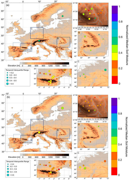
Figure 1.
Normalized temporal median in situ soil wetness index in the top soil layer (0–6 cm) of each station of the growing periods (March–September). (a) 2021; (b) 2022. Coloring of the markers denotes the median soil moisture content, whereas the marker size indicates the temporal interquartile range over the growing period. The background map shows the elevation based on the EU-DEM 25. In situ measuring stations of the following networks are shown in A: REMEDHUS, B: RSMN, C: ICOS, and D: XMS-CAT, SMOSMANIA, and ICOS.
2.2. Data Evaluation
2.2.1. Absolute vs. Normalized Dynamics
All data were processed to represent 3-day running means of the absolute and normalized soil moisture. Absolute soil moisture means the volumetric soil moisture content as provided in all datasets and is expressed in m3m−3. Scaled soil moisture represents the wetness index of the soil. It was calculated using the following the approach of [63] but using the minimum and maximum values from the quality-checked time series before calculating the 3-day running means. This gives us the observed, modeled, or retrieved dynamic ranges for the joint vegetation periods 2021 and 2022 for each grid cell or station [33] as follows:
where is the normalized soil moisture value at time , is the absolute soil moisture at time , and and are the absolute minimum and maximum values of the time series used. We note here that this does not indicate representing the full dynamic range, as there may be sites where neither value represents the corresponding extremes, but it brings the datasets into the same scaled space.
Absolute values are commonly used in soil moisture product comparison studies, such as those conducted within the SMAP community (e.g., [26,34,42]), making it a familiar and widely accepted metric. However, a drawback of the absolute values is that they compare amounts of moisture without accounting for the soil texture or other site-specific factors, which can result in differing value ranges between residual, wilting point, and saturation soil moisture. This means that users, such as farmers or hydrologists, require additional external information to contextualize the absolute values to infer the soil wetness index of a soil and make informed decisions about their specific site. Scaling offers the benefit of comparing value ranges independent of upper and lower limit assumptions, allowing for a direct assessment of the wetness state in the different datasets.
2.2.2. Statistical Measures
The 3-day running means form the basis for all statistical assessments. These include comparisons of the temporal medians computed over the growing periods 2021 and 2022, as well as exploring the periods’ deviations in temporal dynamics using a suite of statistics. An elegant way to visualize these statistics is through Taylor diagrams [64]. They originally combined the Pearson correlation coefficient with the unbiased root mean square difference (ubRMSD) and the standard deviation. The correlation coefficient is essentially a normalized measure of the covariance between the time series. The ubRMSD provides a value for the unbiased mean difference between the measured and the predicted values. The standard deviation quantifies the variability of the values about their mean within the datasets. However, the ubRMSD and the standard deviation assume normal distribution in the data, and different soils, such as sand or clay, may cause skewness in the data due to lags in their wetting and drying phases. To account for this skewness, we replaced the standard deviation with the interquartile range (IQR) in the Taylor diagrams and showed the ubRMSD separately. Consequently, the diagrams cease to be Taylor plots in the original sense, which is why we call them polar plots, but they still provide a visual quantification of the similarity between the time series measured at the stations and those simulated for the cell in the ECMWF operational analysis or retrieved within the SMAP product, respectively. To overlay the reference point of all stations in the diagram, we normalized the IQR by dividing by the IQR of the respective in situ measurement. The normalized IQR (nIQR) has the additional advantage of providing a measure of how much the temporal variability is underestimated (nIQR < 1) or overestimated (nIQR > 1).
In addition to commonly used statistics, such as the difference between gridded and in situ data (calculated by deriving the differences between the time series and averaging over the differences), ubRMSD, and Pearson correlation coefficients, we apply a signal decomposition to disentangle and compare magnitudes of short-term and intermediate-term fluctuations in all soil moisture time series. These are based on the 3-day running mean time series for every year individually. The full time series can be decomposed into a long-term trend spanning over several years, seasonality , and a residual , representing short-term fluctuations [65]. Since we investigate seasonal time series, the long-term trend component is not present in the time series, leaving us with . At first, a 31-day centered running mean is computed from the full time series to derive the seasonality component and decompose the signals. In a second step, the seasonality is subtracted from the full time series to isolate the short-term fluctuations. From these two decomposed time series, we estimate the seasonality strength [66] as follows:
This represents the share of the variability in the time series explained by the seasonality. Hence, a seasonality strength of 0 shows no seasonality, and all variability arises from short-term fluctuations, whereas a seasonality strength of 1 signifies that all variability originates from seasonality. These will be used to compare the standard deviations of the original time series, as well as the seasonality and the short-term fluctuation, to understand over which temporal scale the deviations in the representation of the soil moisture temporal dynamics occur. The IQR is computed for the original and the decomposed time series to receive insight into the magnitude of over- or underestimation and the origin of deviations in the temporal dynamics. The composition of statistical measures gives an overview of the relative skill of the gridded datasets to provide an accurate estimate of the soil moisture dynamics in the cell each station is located in.
2.3. Growing Periods of 2021 and 2022
Since the aim of the study is to investigate the performance of satellite-retrieved and simulated soil moisture for years with different meteorological situations, we selected the two years 2021 and 2022. While 2021 was the first wet year in Europe after the 2018–2020 drought, 2022 was again a drought year characterized by hot and dry conditions in most parts of Europe. The following two paragraphs summarize the meteorological conditions of the two years based on the State of the Climate in Europe reports for 2021 and 2022 by the World Meteorological Organization (WMO) [67,68] and therewith provide the basis for the discussion of the results.
2.3.1. Hydrometeorological Conditions in 2021
In 2021, Europe underwent an extensive warm anomaly in the 2 m temperature of, on average, 1.44 K warmer conditions with little spatial variability across Europe compared to the period 1961–1990 (the official reference period used in the WMO reports changed from 1981–2010 to 1991–2020 between 2021 and 2022; however, we only refer to 1961–1990). Only a small region in northwestern Russia saw below-average temperatures. Particularly large warm anomalies were recorded over the European part of the Arctic and southeastern Europe [68]. In terms of precipitation, 2021 was wetter than the preceding three years but with much larger regional differences than in the temperature observations. That year was dominated by large-scale weather patterns that transported moist Atlantic air from the west or southwest to Europe, leading to wet episodes, which were alternated by north to northeastern circulations transporting cooler air to Central Europe, leading to more pronounced single rainfall events [68]. Dry high-pressure-dominated episodes occur rarely and only for short periods. Consequently, a wet anomaly was observed in northern Scandinavia and large parts of Eastern Central Europe. Especially, large amounts were found in southeastern Europe around the Black Sea. Conversely, dry anomalies were recorded over the Iberian Peninsula. A variety of extreme precipitation events occurred in different parts of Europe in 2021. The heavy precipitation event that affected our study area corresponds to an event that occurred in mid-July over Central Europe, where between 100 and 150 mm of rain fell over an already saturated region, resulting in one of the most severe recorded floods in Germany and Belgium. Other heavy precipitation events occurred in 2021, but they happened either outside the growing period or did not occur close to our measurement sites.
2.3.2. Hydrometeorological Conditions in 2022
Europe overall saw its warmest summer on record in 2022, and record high temperatures were measured in several countries. From the beginning of the growing period in March until the middle of September, long episodes with either high-pressure systems over Europe or anticyclonically oriented large-scale weather patterns dominated. The former led to extended periods of dry and sunny weather, causing prolonged heat and drought conditions in wide areas of Europe [67]. The latter weakened or re-directed moist disturbances, so that they either reached Europe strongly attenuated or even bypassed large parts of Europe. The year was, on average, 1.83 K warmer than the reference period 1961–1990. Nevertheless, compared to 2021, the spatial variability of the temperature anomalies is larger. While Western and southwestern Europe, as well as northwestern Russia, were clearly warmer than the reference, Scandinavia and large parts of Eastern Europe faced a smaller warm anomaly. Cold anomalies were not found over continental Europe. Drought affected much of Europe throughout the year 2022 [67]. In spring, precipitation and soil moisture deficits affected broad regions of Europe (apart from the Iberian Peninsula). The drought conditions reached a peak at the beginning of August. On average, large parts of Europe received below-average precipitation amounts, making 2022 the fourth dry summer in five years after three drought years in 2018, 2019, and 2020. The largest precipitation deficits were found in southern France, and it was the fourth year with a dry anomaly in a row for the Iberian Peninsula. However, several locations in Southern Europe faced heavy precipitation and flooding events, but none of them were close to the in situ network locations chosen for this study, or they occurred outside the principal growing season, such as the heavy rainfall events in over eastern and central Spain in November 2022.
2.4. Domain and Sub-Region Characteristics
Europe is characterized by a large diversity in climates and eco-regimes [69]. They range from an Arctic climate in northern Scandinavia over an oceanic climate, which is influenced by the North Atlantic Current at the Atlantic coast from Portugal to Norway, and continental climates in Eastern Europe to a Mediterranean climate in the south, where the Mediterranean Sea provides moisture for precipitation mainly during the winter season and which is impacted by subtropical winds. Between Scandinavia and Central Europe, the Baltic Sea provides maritime climates in the lowlands. This section introduces the diverse conditions, the networks, and stations chosen for reference measurement.
The focus region, Western Europe, covers the entire Iberian Peninsula and southern France (see Figure 1) and hosts three soil moisture networks, which are frequently used for the validation of remotely sensed soil moisture: the REMEDHUS network in Central Spain, as well as the SMOSMANIA network in southern France and the XMS-CAT network in northern Spain surrounding the Pyrenees. Additionally, it includes the ICOS station Bilos (listed under Western Europe—Rest). Most of the sub-region has a continental semi-arid Mediterranean climate [70], which is characterized by warm temperatures, low summer precipitation, and a weak buffering influence of the Atlantic Ocean [69,71]. REMEDHUS is considered one of the core validation sites for soil moisture globally [26]. The network is in the Duero Basin, which is an agricultural area with mostly rainfed crops [70] and mainly sandy soils [72]. The SMOSMANIA network is in the north of the Pyrenees. Stations were set up under the avoidance of mountainous areas as much as possible [73] and dedicated to cover measurements across the transect between the Atlantic coast and the Mediterranean Sea. The Lusitanian environmental zone close to the Atlantic coast experiences higher oceanicity, warm to hot temperatures, and more precipitation, which usually results in sufficient water availability. Stations close to the Mediterranean Sea experience a Mediterranean climate. All SMOSMANIA stations are located over formerly cultivated fields, which are now covered with regularly cut grassland [73,74]. The soil textures vary between sandy soils at the Atlantic coast and the northeastern cluster of the SMOSMANIA network, as well as rather loamy soils [74]. The XMS-CAT network was established in the south of the Pyrenees. The climate again is Mediterranean, and the measurement sites are located either in shrubland or between vineyards in relatively hilly areas. Soil textures range between loam and clay loam (https://visors.icgc.cat/mesurasols/#9/42.1765/1.1132, last accessed 16 January 2025).
The stations in Central Europe (as well as those in Davos in the Alps and Hyytiälä in Finland, which are not contained in the Central Europe focus region) are part of the ICOS network [62]. The focus region generally has flat terrain. The Atlantic climate in the west of Central Europe is characterized by strong ocean buffering and thus mild winters and moist cool summers. Oceanicity decreases toward the east, causing a higher seasonality in temperature variations. Precipitation largely occurs during the summer months [71]. The Belgian stations are agricultural areas or forested (Vielsalm). Similarly, the German station (Hohes Holz) is located within a forest, which itself is surrounded by crop fields.
Finally, the RSMN network in Eastern Europe is distributed across Romania. The Romanian lowlands, where most of the considered stations are located, are dominated by a relatively flat, steppic character, exhibiting a warm temperate, continental climate. Precipitation mainly occurs early in the summer, which can lead to water shortage later in the year [71]. The highest temperatures and lowest amounts of precipitation occur in the South and East of the country [36], closer to the coast of the Black Sea. The land cover is dominated by rainfed agricultural land use with few forests. The remaining stations are depicted under “Europe-Rest”.
3. Results
3.1. Mean In Situ Soil Moisture and Its Drivers
Figure 1 shows the normalized median and interquartile ranges over time for each site for 2021 and 2022. The lower median soil moisture in 2022 at all stations, except for REMEDHUS El Tomillar, SMOSMANIA Pezenas, and XMS-CAT La Cultia d’Areu and Ribera de Sio, reflects the overall drier conditions in 2022.
The REMEDHUS exhibits the driest conditions across all regions in both years. The stations show absolute median volumetric soil moisture contents ranging between 0.006 m3m−3 and 0.23 m3m−3 in 2021 and between 0.003 m3m−3 and 0.18 m3m−3 in 2022 (see Figure A1). The lowest median volumetric soil moisture contents occur at the stations with the highest sand fractions (El Coto, El Tomillar, Las Brozas; see Figure A2), and the higher median soil moisture contents occur at the stations with larger clay fractions (Canizal, Guarrati, Las Arenas) in both years. The normalized median soil moisture exhibits values below 0.5 at all stations but Canizal, suggesting that the REMEDHUS network faced dry (0.25–0.5) or very dry (<0.25) soil moisture conditions in 2021 (see Figure 1a). In 2022, all stations except for Canizal showed normalized soil moisture of below 0.2, indicating very dry soil moisture conditions. Similar behavior occurs at the SMOSMANIA and XMS-CAT networks located around the Pyrenees. Absolute soil moisture values vary between 0.05 m3m−3 and 0.23 m3m−3 in 2021, which means mildly dry to very dry soil moisture states across the networks, as indicated by the normalized soil moisture. In 2022, the soils dry to a range of 0.004 m3m−3 and 0.2 m3m−3, which implies very dry median wetness conditions around those networks in 2022. In Central Europe and Eastern Europe, all stations show mildly dry to mildly wet soil wetness (the normalized median soil moisture of the stations varies between 0.43 and 0.67) in 2021. Analogously to the other networks, soils are drier in 2022, with normalized median soil moisture ranging between 0.17 and 0.47.
3.2. Comparison of Average Soil Moisture Between In Situ Measurements and Cell Data
Here, we examine differences in the median soil moisture content and soil wetness index between the in situ measurements and the cells of the gridded data, where each station is located. Figure 2 shows the median absolute soil moisture content plotted against the difference between the median of the respective gridded cell and the median of in situ measurements of each station for the soil moisture contents. In contrast, Figure 3 displays normalized soil moisture, indicating the respective soil wetness index. Both ECMWF and SMAP DCA overestimate soil moisture contents at most stations (positive difference), in particular for drier soils. The wet bias in the ECMWF operational analysis is stronger (2021: 0.111 m3m−3; 2022: 0.114 m3m−3) than in SMAP DCA (2021: 0.055 m3m−3; 2022: 0.053 m3m−3) (see Figure 4a). The maximum difference can reach up to 0.29 m3m−3 for ECMWF at an XMS-CAT station and up to 0.23 m3m−3 for SMAP DCA at the Finnish station in 2021. The RMSDs and ubRMSDs of SMAP are smaller than those of the ECMWF (see Figure 4c,d).
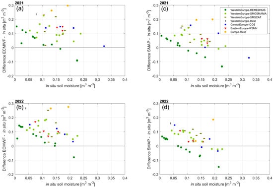
Figure 2.
Median station soil moisture plotted against the difference between the median of the in situ measurement and the median of the ECMWF time series in 2021 (a) and 2022 (b). Subplots (c,d) show the same for the difference in medians between in situ and SMAP DCA. The different markers denote the region and network of each station.
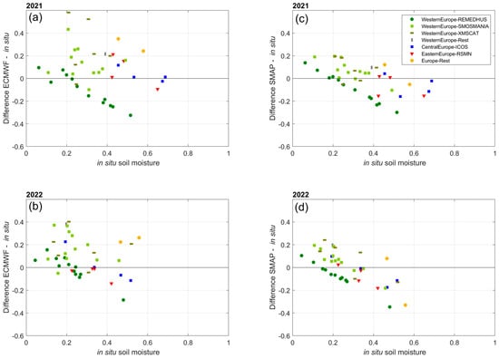
Figure 3.
Normalized median station soil moisture plotted against the difference between the normalized median of the in situ measurement and the normalized median of the ECMWF time series in 2021 (a) and 2022 (b). Subplots (c,d) show the same for the difference in medians between in situ and SMAP DCA. The different markers denote the region and network of each station.
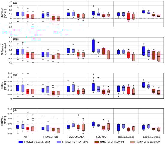
Figure 4.
Detailed statistics of the time series. (a) Differences in absolute soil moisture content [m3m−3]; (b) difference in normalized soil moisture; (c) RMSD of the absolute soil moisture contents; (d) unbiased RMSD of the absolute soil moisture contents. The colors indicate the dataset. Blue: ECMWF vs. in situ 2021, pale blue: ECMWF vs. in situ 2022, red: SMAP DCA vs. in situ 2021, pale red: SMAP DCA vs. in situ 2022. Dashed whiskers represent 2.7 times the standard deviation and plus sign indicates outliers.
A comparison of the soil types classified in the model, the grain size distribution in the soilGrids dataset used in SMAP, and the grain size distribution assessed at each station revealed discrepancies (see Figure A2) between the soil types of the in situ, model, and remote sensing data. This mismatch implies differences in the dynamic ranges of the datasets and systematic shifts that can be attributed to varying lower and upper limitations for the soil moisture values. Additionally, the ecLand model applies the permanent wilting point as a lower limit assumption, whereas in reality, soil moisture values can reach below the wilting point, extending down to the residual moisture content. To account for these differences, we normalized the time series data using their respective minimum and maximum values over both vegetation periods.
Comparing Figure 2 and Figure 3 shows that the discrepancies in soil types and lower and upper limit assumptions explain parts of the wet errors, as points appear to scatter more around the zero line (see Figure 3) and show reduced systematic trends. The decrease is particularly evident at the stations in Central Europe—Rest, and Eastern Europe. In the latter case, the majority of points get closer to zero in both years, indicating the removal of a systematic bias between the soil moisture values at those sites through normalization. At the sandy stations of the REMEDHUS network, the normalized soil moisture reports too dry soil wetness indices in SMAP, whereas the ECMWF data cluster more around the zero line. In the SMAP data, the absolute error of the normalized data appears even larger than the non-normalized soil moisture content due to scaling to the dynamic range. Highlighting the impact of differences between soil types, the stations with the driest signals (both in absolute and normalized terms) show the biggest positive differences, which can also be reinforced due to sandy soil type (see Figure A2, e.g., for REMEDHUS), and the tendency decreases with increasing in situ soil moisture (see Figure 2 and Figure 3). This behavior is consistent for both ECMWF and SMAP for 2021 and 2022, regardless of the region or network. The data points of the different networks and regions nicely cluster around diagonals, with the strongest clustering in REMEDHUS. This rather systematic pattern may indicate that the differences are governed by the value distribution of the observations.
3.3. Comparison of Temporal Variability of Gridded Cells Against In Situ
Figure 5 shows statistical measures comparing ECMWF and SMAP against in situ averaged over the focus regions and networks, respectively. Figure 6 and Figure 7 present comparisons of ECMWF and SMAP time series for the individual stations. The left column of each panel depicts the points for 2021, and the right column depicts the points for 2022. Those plots visualize the comparisons of the decomposed statistics of the soil moisture signals in terms of the correlation coefficients of the seasonality between in situ measurements and the respective gridded dataset in the top row and those of the short-term fluctuations in the bottom row.
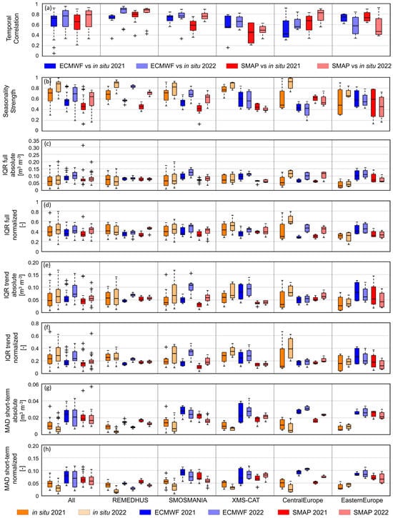
Figure 5.
Statistics of the time series temporal variability. (a) Pearson correlation coefficient; (b) seasonality strength; (c) interquartile range of the full time series of soil moisture content; (d) interquartile range of the full time series of the normalized soil moisture; (e) interquartile range of the seasonality of soil moisture content; (f) interquartile range of the seasonality of the normalized soil moisture; (g) median absolute deviation of short-term fluctuations—soil moisture content; and (h) median absolute deviation of short-term fluctuations—normalized soil moisture. The colors indicate the dataset. Blue: ECMWF 2021, pale blue: ECMWF 2022, red: SMAP DCA 2021, pale red: SMAP DCA 2022, in situ 2021: dark orange, in situ 2022: pale orange. In (a), the colors represent the respective dataset compared against the in situ time series of the same year. Dashed whiskers represent 2.7 times the standard deviation and plus sign indicates outliers.
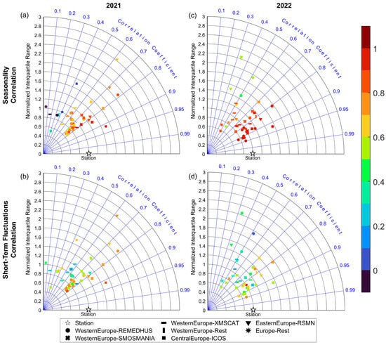
Figure 6.
Polar plot depicting the similarity of the full time series of the in situ observations with the respective cell in the ECMWF operational analysis. (a) Depicts the comparison in terms of the normalized interquartile ranges and the temporal correlation coefficients of the full time series between ECMWF and the in situ observations for the growing period 2021. The different markers indicate the focus region. In Western Europe, the markers additionally distinguish the three networks. The colors represent the Pearson correlation coefficient between the seasonality of the in situ observation and the cell from the ECMWF analysis. (b) Shows the same data points as (a), but they are colored in terms of the correlation between the time series of the short-term variability from in situ and ECMWF analysis. (c,d) Show the same configuration but for the growing period 2022.
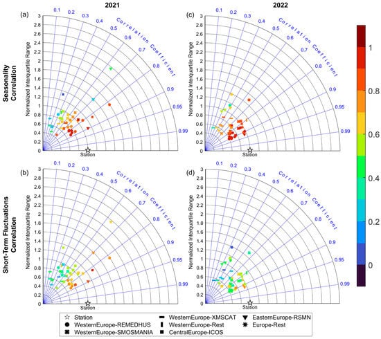
Figure 7.
Polar plot depicting the similarity of the normalized full time series of the in situ observations with the respective cell in SMAP DCA. (a) Depicts the comparison in terms of the normalized interquartile ranges and the temporal correlation coefficients of the full time series between SMAP and the in situ observations for the growing period 2021. The different markers indicate the focus region. In Western Europe, the markers additionally distinguish the three networks. The colors represent the Pearson correlation coefficient between the seasonality of the in situ observation and the cell from SMAP. (b) Shows the same data points as (a), but they are colored in terms of the correlation between the time series of the short-term variability from in situ and SMAP. (c,d) Show the same configuration but for the growing period 2022.
The gridded datasets show several common differences in their deviations from the in situ measurements. Firstly, both gridded datasets show high similarity in the timing of the temporal dynamics with the in situ measurements. Deviations between the temporal correlations of ECMWF or SMAP with in situ (see Figure 5a) are negligible. The magnitudes of temporal variability represented by the IQR of the time series of absolute soil moisture contents are overestimated at 33/42 for ECMWF and 23/42 of the stations for SMAP (see Figure 5c). The largest and statistically significant overestimations of the temporal variability (p < 0.05) occur in Eastern Europe and SMOSMANIA for both growing periods in ECMWF (see Figure 5c). In Eastern Europe, the observed temporal variability is low due to both weak seasonality (see Figure 5e,f) and weak short-term variations (see Figure 5g,h). Both SMAP and the ECMWF operational analysis show stronger seasonality and short-term variability (potential reasons will be further discussed in Section 3.4.2). After normalization, the IQRs become more aligned. None of the sub-regions and vegetation periods show statistically significant differences in the comparison of ECMWF with in situ data. In comparison with SMAP, REMEDHUS in 2021 and Central Europe in 2022 show significantly drier soils than measured in situ. The median nIQRs of all regions drop below 1 everywhere apart from Eastern Europe (see Figure 5c,d), which indicates that the overestimation of the temporal variability in the gridded datasets can be in part attributed to differences in the dynamic ranges for normalization. The stations in Central Europe form an exception regarding the alignment due to normalization in 2022, and the soils show a significantly drier state, though the absolute soil moisture contents were in a similar range in all datasets (see Figure 5c,d).
A second common feature is that the gridded datasets consistently underestimate the seasonality strength, with larger underestimations in SMAP than in ECMWF in both years (see Figure 7b). In the in situ data, the seasonality constitutes the larger part of the temporal variability, indicated by a median seasonality strength of 0.71 across all in situ measurements in 2021 and 0.88 in 2022. This reflects the typical intra-annual climatic changes in the extratropics and high latitudes.
The seasonal trends of all soil moisture time series are mostly in the same range (see Figure 5e,f) and correlate well in both ECMWF and SMAP, which is indicated by the orange and red colors of the markers in the top rows of the Taylor diagram panels denoting correlation coefficients > 0.7 (see Figure 6a,c and Figure 7a,c). In contrast, short-term variability is less correlated (blue and green markers showing low to moderate correlations; see Figure 6b,d and Figure 7b,d). The IQR of the time series in the gridded dataset suggests too large short-term variations across the stations (see Figure 5g,h). This is a consistent feature in all sub-regions, which is also present after normalization (see Figure 5g,h). The overestimation of the short-term variability leads to a shift towards lower seasonality strengths in the gridded datasets in all regions, but particularly in XMS-CAT and Central Europe.
This leads finally to the common differences between the years. The dry and hot growing period of 2022 is characterized by strong seasonality, weak short-term fluctuations, and thus a large seasonality strength across all focus regions and networks in the in situ measurements (see Figure 5c–h). The warm and humid growing period in 2021 showed lower seasonality but stronger short-term fluctuations, which resulted in a weaker seasonality strength. The larger seasonality strength in 2022 could only be captured by the gridded products at the REMEDHUS and SMOSMANIA stations (see Figure 5b). At the XMS-CAT and Central Europe stations, the lower seasonality strength observed in 2022 compared to 2021 in the gridded datasets can be attributed to a combination of too weak an increase in seasonality and a concurrent rise in short-term variability (see Figure 5e–h). In Eastern Europe, the gridded datasets show a weaker seasonality in 2022 than in 2021 and minor changes in the short-term variability. Both datasets show mostly larger temporal correlations and a lower overestimation of the IQR in 2022.
Nevertheless, there are also differences in the deviations of the gridded datasets from in situ measurements. The overestimation of the magnitude of temporal variability of the absolute value time series is stronger in ECMWF than in SMAP (see Figure A3 and Figure A4). In contrast, the evaluation of the ECMWF data overall shows larger temporal correlations with the in situ measurements, implying slightly better timing of the temporal dynamics (see Figure 5a). The exception in both cases is the stations in Central Europe.
3.4. Time Series
3.4.1. Dry Conditions and Dry Down Phase
This section explicitly examines the representation of dry down and drought periods based on the Concejo del Monte station from REMEDHUS (see Figure 8) and demonstrates the impact of the lower and upper limit assumptions in the gridded dataset on the absolute soil moisture time series. The vegetation around the station is rainfed crops, and the dominant vegetation type in the IFS model is cropland. The area covered by the grid cell in the model and the satellite product has a 96% crop cover based on Sentinel-2 data [75]. The homogeneity in land cover allows better comparability between the in situ measurements and the gridded products. The station was exemplarily chosen as it faced persistent dry periods where the top soil moisture content approached minimum soil moisture values and fell below the wilting point in the in situ measurement. For this particular station, the IFS data was closest to the in situ measurement during wet phases, whereas SMAP performed better in the dry down and dry phases. Meteorological measurements were provided by the site hosts for four weather stations in the REMEDHUS area [76].
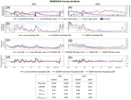
Figure 8.
Decomposed 3-day running mean time series of soil moisture and air temperature, as well as daily accumulated precipitation, at the REMEDHUS station, Concejo del Monte. The top row shows the 3-day running mean in situ soil moisture (black, solid) and temperature (purple, solid), their seasonality (dashed), and daily accumulated precipitation. The second row shows the normalized soil moisture time series of the in situ station (black), the cell in ECMWF (blue), and SMAP DCA (red). The third row shows the in situ soil moisture time series and seasonality plotted against those of the cells in ECMWF (blue) and SMAP DCA (red), containing the in situ station. The bottom row shows the short-term variability of all time series plotted against each other. The left plots show the growing period of 2021 (a–d), and the right plots show the growing period of 2022 (e–h).
In 2022, the station experienced a long dry down phase as a consequence of a lack of precipitation events between the end of April and the beginning of August (see Figure 8e). Both gridded datasets capture a dry down phase. However, SMAP was too dry in the spring months, approaching the in situ measurements during the dry phase. ECMWF was too wet in spring, converged with the measurements in May, and then it diverged again as it was approaching its parameterized permanent wilting point ([51], Table 8.9). This assumption prevents the model from drying beyond the wilting point through plant transpiration. Soil evaporation allows further drying from non-vegetated areas until the residual soil moisture, leading to a minimum soil moisture for the grid cell corresponding to the vegetation fraction-weighted average of the wilting point and residual soil moisture content of the respective soil type [77]. In theory, the model could be initialized below the wilting point through the data assimilation framework of the IFS. The permanent wilting point is given for each soil type, and the soil texture map provides the info of which type prevails in the cell. Cells covering the locations of the REMEDHUS stations have the medium soil texture type in the IFS soil texture map with a permanent wilting point of 0.151 m3m−3. Since the cells containing REMEDHUS stations mostly contain crops having a vegetation fraction of 90%, this is almost the value at which the soil moisture content evens out in the ECMWF time series. Similarly, a hard-coded value range exists in the SMAP product, which provides a relaxation of the boundary conditions for the retrieval algorithm. This is set to 0 m3m−3 as the lower limit and 0.6 m3m−3 as the upper limit independently of the soil texture [44]. Despite this difference, the time series show large agreements in the seasonality and the short-term variability (see Figure 8c,d,g,h).
3.4.2. Variability Overestimation in Eastern Europe
As reported in the previous sections, the largest deviations in representing the soil moisture dynamics in gridded datasets occur in Eastern Europe. Both gridded datasets overestimate the absolute soil moisture content and the temporal variability compared to the in situ measurements. This chapter evaluates factors influencing the overestimation of mean soil moisture and soil moisture dynamics in Eastern Europe based on the station Satu Mare (see Figure 9).
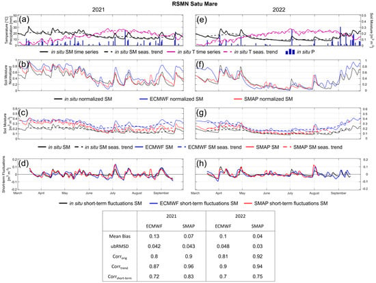
Figure 9.
Decomposed 3-day running mean time series of soil moisture and air temperature, as well as daily accumulated precipitation, at the RSMN station, Satu Mare. The top row shows the 3-day running mean in situ soil moisture (black, solid) and temperature (purple, solid), their seasonality (dashed), and daily accumulated precipitation. The second row shows the normalized soil moisture time series of the in situ station (black), the cell in ECMWF (blue), and SMAP DCA (red). The third row shows the in situ soil moisture time series and seasonality plotted against those of the cells in ECMWF (blue) and SMAP DCA (red), containing the in situ station. The bottom row shows the short-term variability of all time series plotted against each other. The left plots show the growing period of 2021 (a–d), and the right plots show the growing period of 2022 (e–h).
The in situ measured soil moisture content barely reacts to the meteorological conditions in 2021 and 2022, shown by weak seasonality and low peaks following precipitation events (see Figure 9a,d). Measured short-term variability is low, which is a common feature among all the Romanian stations. The gridded datasets both show a stronger seasonality (see Figure 9b,e) and amplified short-term variability (see Figure 9c,f). The peaks and lows of the time series mainly have the right timing, which is supported by intermediate to high temporal correlations (see Figure 5a), but the amplitude of the fluctuations is severely overestimated (see Figure 9d,h). The latter is also shown by statistically significantly larger median absolute deviations both in the absolute soil moisture content and in the normalized soil moisture.
Comparing the response of the soil moisture content to the occurrence of precipitation events between the Concejo del Monte (see Figure 8a,e) and the Satu Mare station (see Figure 9a,e) results show that the soil moisture content at the Romanian station exhibits a lower sensitivity to precipitation events in the measured time series. One possibility is that the local sensor calibration is incorrect, which could be indicated by the measured soil moisture in general being below the expected wilting point for this type of soil. The soils at many of the Romanian stations have comparatively high fractions of clay and silt and should, therefore, have an observed range of higher soil moisture. One factor on the model side is the soil texture classification and the parameterization of the soil type. In ECMWF, soils are classified as medium or medium-fine in the grid cells hosting Romanian stations and, therefore, have medium to high porosity. At two of the four stations, including Satu Mare, the soil texture does not lie in the span of the classified soil type in ECMWF (see Figure A2). Differences in the soil texture also influence, e.g., the hydraulic conductivity and the infiltration rate to the soil at these stations, which are calculated in dependence on the soil texture using pedotransfer functions [78]. In ECMWF, the coarser textures have higher hydraulic conductivities and higher infiltration rates than finer ones [50]. It is possible that a mismatch between the model’s local soil texture and that at the station could lead to too much water infiltrating the soil instead of running off at the surface. With the Hortonian runoff formulation, the land surface scheme of the IFS system uses an excess infiltration formulation to derive runoff by balancing the rates of precipitation and melting with the infiltration rate [79]. Amongst other things, the infiltration rate of soils is a function of the soil water content and decreases with an increasing degree of saturation [80]. Consequently, an initially dry soil with a relatively coarse soil texture will have a high infiltration rate and soil conductivity, leading to rapid soil wetting in the modeled top layer and relatively weak losses of water through runoff. In contrast, finer soils, like loams and clays, have lower soil conductivity and, in reality, can face surface sealing, which would promote surface runoff [51]. For the stations with a mismatch between local and parameterized soil texture, this could, in turn, lead to an increased storage of water in the soil and higher soil moisture dynamics at the affected stations. This would cause an overestimation of the short-term fluctuations and also the median soil moisture content itself. Another potential influence in the IFS is the coupled data assimilation scheme, which may lead to an artificial increase in soil moisture due to atmospheric water demand. In any case, this highlights that a mismatch in the assumptions of the soil texture information can lead to significant differences between the two soil moisture products.
4. Discussion
All assessments in this study were conducted for the wet growing period in 2021 and the drought-affected growing period in 2022 across European measuring stations. Firstly, it must be acknowledged that in situ soil moisture is measured at the point scale, whereas both the model and the satellite remote sensing products represent a spatially integrated value for the respective resolution cell. Unless one has a representative soil moisture monitoring network to properly reflect the mean behavior of the grid area, which would be prohibitively expensive to achieve due to the spatial heterogeneity of the soil, uncertainties in the direct comparison among the datasets need to be considered [37]. Furthermore, differences in the actual vegetation at the station and the dominant vegetation types defined for the grid cell can influence the soil moisture dynamics, in particular dry down behavior, due to differences in the vertical root distribution and the consequent plant water uptake from different soil depths. While vegetation types with shallow roots, such as most grasses, extract almost all their required water from the topsoil, deciduous forests can also extract water from deeper soil layers, for example [51]. Large plant water uptake from the topsoil intensifies the top-layer dry down and thus contributes to discrepancies in the topsoil moisture timeseries under drought conditions. Another source of uncertainty for the comparison is the slightly different soil moisture sensing depths. In situ observations are measured at discrete soil depths between 4 and 6 cm under the soil surface, assuring the probe is sufficiently covered by topsoil. The modeled values are integrals for one layer between 0 and 7 cm, and the satellite remote sensing retrievals at the L-band are mostly sensitive to soil moisture until ~5 cm, although Feldman et al. pointed out that at the L-band frequency, remote sensing-based soil emission can carry information from deeper depths if connected [39]. Though these differences are not that large in absolute cm, the main uncertainty arises from the circumstance that modeling and remote sensing represent integral values, which also include the top 1–2 cm reacting more sensitively to, e.g., light precipitation. For this reason, and to improve comparability with remote sensing products, ECMWF’s next-generation land surface model, ECL, thus introduced a higher vertical discretization of the soil [58]. The in situ probes measured at a discrete depth below these 1–2 cm can cause weaker variability compared to the integrated soil moisture. Hence, the limitation of the findings discussed in this study is the assumption that soil moisture does not change drastically within the shallow soil layer between 0 and 7 cm (i.e., in the order of 0.3 m3m−3 or more). However, following the assumption that anomalies account for these differences (spatial coverage, measuring depth), we normalized the data and compared soil moisture in normalized terms (soil wetness index) in addition to the absolute value time series for comparison against previous studies. In the end, a comparison of topsoil in situ, model, and satellite retrievals remains the de facto standard for the assessments as presented in this paper.
Generally, the two gridded datasets show high similarity in their temporal dynamics and common deviations from the in situ measurements (see Figure 5, Figure 6 and Figure 7). Ref. [34] showed that satellite remote sensing-based products improved during the last years and show similar temporal correlations with in situ data as the model-based data. This was attributed to substantial improvements in the space-borne soil moisture retrievals, which were also reported by [35]. In our study, SMAP exhibits a higher accuracy in the absolute values of the growing periods across Europe, which is shown by consistently smaller differences and lower ubRMSDs everywhere, except for the SMOSMANIA network in 2021 (see Figure 4). Both gridded datasets exhibit a wet bias at most stations when comparing the absolute values, which is, on the one hand, linked to the assumptions (e.g., wilting point as lower limit), whereas the top soil can dry out, reaching the residual soil moisture in the end. Additionally, the soil moisture content responds to coupled data assimilation by compensatively adding or removing soil moisture when and where needed in ECMWF, which can lead to soils being too wet in the vegetation period [81], for models with too little transpiration that cannot meet the atmospheric water demand.
Interestingly, grid cells containing stations with low amounts of soil moisture show positive differences, whereas stations with higher amounts of moisture also show negative differences in both ECMWF and SMAP (see Figure 2), which was also found by [31] for several reanalysis datasets. The inverse proportionality of in situ soil moisture and the difference between gridded data in situ measurement is present in both datasets and within all focus regions and networks during both growing periods. The same signal, but more moderate, is also shown in the normalized soil moisture comparisons (see Figure 3). This implies that stations with generally drier soils are misrepresented in the model as being too humid, whereas stations with moderately humid conditions tend to be too dry in the gridded datasets. One factor in this could be the scale mismatch, where model and satellite retrieval pixels generally have the dominant soil type as being the representative one, which is usually closer to an average condition under the assumption of homogeneity within the pixel.
The performance of timing is comparable (degree of temporal correlation of SMAP and ECMWF with in situ). The correlations between ECMWF and in situ are, on average, slightly higher, but differences between the correlations of ECMWF and SMAP with in situ are statistically non-significant (see Figure 5a). Good agreement in timing was also found in previous studies for both remote sensing and model-based soil moisture products [28,30,31,34,53]. Our comparisons add the magnitudes of the temporal variability (nIQR), which is predominantly overestimated for the absolute soil moisture contents but shows a similar degree or an underestimation for the variability in the soil wetness indices (normalized soil moisture). The stations in Eastern Europe stood out with, in part, large overestimations of the temporal variability in absolute and normalized terms in both gridded datasets compared to the in situ measurements (see Figure 6 and Figure 7). Parts of the deviations may be associated with the missing calibration of the soil moisture sensors at the measurement sites. However, several studies (e.g., [31,36]) also showed that retrievals may be challenging over clay-rich soils as present at the stations in Eastern Europe [82].
The tendency towards higher temporal correlations and lower ubRMSD in 2022 demonstrates better performance in periods with low soil moisture due to a lack of short-term variability in the time series. In 2022, the persistent heat and drought conditions forced continuous drying and resulted in a strong seasonality, whereas the rare occurrence of precipitation events initiated little short-term variability. Conversely, in 2021, short-term variability mainly initiated by the occurrence of precipitation events (see Figure 8 and Figure 9); e.g., [83,84,85] contributed to a larger proportion of the temporal variability, while the seasonality was weaker due to the lack of drought conditions. This suggests that in ECMWF episodes with strong seasonality, weak short-term fluctuations can be captured better in terms of both temporal variability and accuracy than wet periods with frequent precipitation events, such as in 2021. For satellite retrievals, the situation is different compared to the model since remote sensing retrievals are based on the measured radiometer brightness temperatures. These are employed to estimate soil moisture by emission modeling and data-injection model inversion. Precipitation events are indirectly recognized as changes in the emission and reflection of the land surface because of the wetting of the soil and the subsequent changes to the dielectric constant of the soil. However, for the model, the lack of short-term variability due to a low frequency of precipitation events in 2022 compared to 2021 reflects better performance of the retrieval during 2022.
Finally, we must acknowledge that the focus on only two years (2021, 2022) limits the generalizability of our findings. We are aware that two vegetation periods cannot reflect the full range of climate variability and thus, hydrometeorological conditions possible at each location over Europe. The focus in this study was on two diverging years (humid year 2021, drought-affected year 2022) to allow in-depth analyses at many stations across Central Europe and due to the varying data availability of remote sensing-based (SMAP), modeling (ECMWF), and in situ measurements. Another limitation for the generalizability is the choice of only two gridded datasets. Despite common assumptions with other soil moisture products from both approaches, the final setup of the ancillary data, such as soil type, vegetation, topographic maps, and other assumptions (e.g., soil parameters for the model system or the dielectric mixing model in remote sensing), produces dataset-specific estimates of the soil moisture [30]. The next steps include, therefore, the analysis of longer time series (including other drought events and wet years) and more datasets to verify findings of this study and to increase our knowledge on the temporal dynamics of soil moisture from remote sensing, modeling, and field observations.
5. Conclusions
Accurate and spatially comprehensive soil moisture information is required for many applications, such as agricultural management, hydrological modeling, process studies on soil moisture-climate feedback, and to accurately initialize forecasts at different timescales [86]. The overarching goal of this study was to evaluate the level of agreement in temporal soil moisture patterns between ECMWF operational analysis and SMAP DCA L3 in relation to in situ measurements across European measuring stations. In order to enable decision makers across various application fields to choose reliably, they need to trust the temporal dynamics of soil moisture, which is achieved by comparing gridded soil moisture products (e.g., SMAP or ECMWF) to in situ measurements based on several statistical parameters. Their combination is supposed to depict various aspects of the temporal dynamics, such as timing and magnitude of variability, and disentangle short-term variability representation from seasonality representation throughout two different hydrometeorological seasons.
In conclusion, despite considerable advancements, particularly in remote sensing-based soil moisture retrieval approaches during the last decade [35], there remains room for improvement. Model parameterizations and satellite retrieval algorithms must capture the soil moisture characteristics for a wide range of locations. Improving the accuracy of the absolute values in the model is challenging, as errors arise from differences in the soil maps, which cannot be easily changed in an operational system, and from non-physical increments in the data assimilation scheme to improve the near-surface atmospheric conditions [81,87]. For the remote sensing soil moisture, errors are associated with the soil temperature and vegetation data fed into the algorithm, which have biases themselves [88], and for all gridded datasets, one needs to consider spatial representativeness errors (spatial scale gap) in comparisons with in situ data. However, given that most stations showed overestimations in the short-term fluctuations, which are influenced by precipitation–evapotranspiration dynamics and vertical water movement, it appears promising to focus on this aspect. It is assumed that mainly humid areas or stations facing humid periods benefit from an improved representation of short-term dynamics.
Our results provide additional insights into reasons for deviations in the model- and satellite-based representation of soil moisture temporal dynamics in models and remote sensing from observations. By acknowledging differences in the comparability of the soil moisture at different temporal scales and under different hydrometeorological conditions, it is possible to develop more effective strategies for informing model-based and satellite-based approaches with each other, e.g., via data assimilation in sub-seasonal to seasonal forecasts or as ancillary data to the retrieval algorithm. Further research can build on these findings and focus on the evaluation of spatial patterns of soil moisture. Ultimately, the choice of soil moisture data should be made with caution, considering ancillary information to unlock the full potential of soil moisture information for the intended analysis and respective application.
Complementary to these temporal dynamics analyses, this study builds the foundation for comparisons of spatial patterns between ECMWF and SMAP soil moisture information in a companion study on spatial patterns [89].
Author Contributions
Conceptualization, L.J. and T.J.; methodology, L.J., D.C. and F.M.H.; software, L.J.; validation, L.J.; formal analysis, L.J.; investigation, L.J.; data curation, L.J., H.-S.B., D.C., A.F., F.M.H. and G.P.; writing—original draft preparation, L.J.; writing—review and editing, L.J., H.-S.B., D.C., A.F., F.M.H., G.P. and T.J.; visualization, L.J.; supervision, T.J. All authors have read and agreed to the published version of the manuscript.
Funding
Lisa Jach acknowledges funding from the Anton and Petra Ehrmann-Stiftung Research Training Group “Water-People-Agriculture” for the guest research stay at DLR Oberpfaffenhofen. Florian Hellwig is funded by the Deutsche Forschungsgemeinschaft (DFG, German Research Foundation)—514721519 by the project “Remote sensing of vegetation canopy properties: States & spatio-temporal dynamics” as part of the DFG Research Unit 5639: Land Atmosphere Feedback Initiative (LAFI). David Chaparro has been funded by the projects “la Caixa” Junior Leader Fellowship LCF/BQ/PI25/12100008 (lead: D. Chaparro) and LCF/BQ/PI23/11970013 (lead: O. Binks) and by the project H2020 FORGENIUS (Improving access to FORest GENetic resources Information and services for end-USers) #862221.
Data Availability Statement
The in situ measurements from the networks (e.g., ICOS, ISMN) and SMAP data are publicly available via the provided references. ECMWF operational analyses are available upon request from ECMWF.
Acknowledgments
The authors sincerely want to thank Christoph Rüdiger, leading the Land ModellingLand Modelling team within the Research Department (Earth System Modelling section) of ECMWF, for his very valuable comments, which substantially improved the manuscript. No generative AI was used for generating this manuscript.
Conflicts of Interest
The authors declare no conflicts of interest.
Abbreviations
The following abbreviations are used in this manuscript:
| AMSR2 | Advanced Microwave Scanning Radiometer |
| ASCAT | Advanced Scatterometer |
| DCA | Dual Channel Algorithm |
| ECV | Essential Climate Variable |
| ECMWF | European Center for Medium-range Weather Forecasts |
| ESA | European Space Agency |
| EUMETSAT | European Organisation for the Exploitation of Meteorological Satellites |
| 4D-Var | Four-dimensional Variation Assimilation |
| ICOS | Integrated Carbon Observation System |
| IFS | Integrated Forecast System |
| IQR | Interquartile Range |
| ISMN | International Soil Moisture Network |
| LES | Large-Eddy Simulation |
| NASA | National Aeronautics and Space Administration |
| MetOp | Meteorological Operational Satellite |
| NDVI | Normalized Differential Vegetation Index |
| SMAP | Soil Moisture Active Passive |
| SMOS | Soil Moisture Ocean Salinity |
| SYNOP | Surface Synoptic Observations |
| ubRMSD | Unbiased Root Mean Square Difference |
| UTC | Coordinated Universal Time |
| WMO | World Meteorological Organization |
Appendix A

Figure A1.
Absolute temporal median of in situ soil moisture [m3 m−3] in the top soil layer (0–6 cm) of each station of the growing periods (March–September) (a) 2021 and (b) 2022. Coloring of the markers denotes the median soil moisture content, whereas the marker size indicates the temporal interquartile range over the growing period. The background map shows the elevation based on the EU-DEM 25. In situ measuring stations of the following networks are shown in A: REMEDHUS, B: RSMN, C: ICOS, and D: XMS-CAT, SMOSMANIA, and ICOS.


Figure A2.
Soil textures for the different stations. The markers indicate the different regions or networks. The stations are grouped according to the soil texture class implemented in the respective cell in the ECMWF operational analysis. The classes are based on the FAO soil texture classification, and the polygon in each triangle denotes the area the respective FAO soil texture class covers [60]. The shaded gray area is the texture space covered by the ECMWF soil texture.


Figure A3.
Polar plots depicting the similarity of the full time series of the absolute soil moisture contents of the in situ observations with the respective cell in the ECMWF operational analysis. (a) Depicts the comparison in terms of the normalized interquartile ranges and the temporal correlation coefficients of the full time series for the growing period 2021. (b) Shows the same data points as (a) but colored in terms of the correlation between the time series of the short-term variability. (c,d) Show the same configuration but for the growing period 2022. The different markers indicate the focus region. In Western Europe, the markers additionally distinguish the three networks. The colors represent the Pearson correlation coefficient between the seasonality of the in situ observation and the cell from the ECMWF analysis.


Figure A4.
Polar plots depicting the similarity of the full time series of the absolute soil moisture contents of the in situ observations with the respective cell in SMAP DCA. (a) Depicts the comparison in terms of the normalized interquartile ranges and the temporal correlation coefficients of the full time series for the growing period 2021. (b) Shows the same data points as (a) but colored in terms of the correlation between the time series of the short-term variability. (c,d) Show the same configuration but for the growing period 2022. The different markers indicate the focus region. In Western Europe, the markers additionally distinguish the three networks. The colors represent the Pearson correlation coefficient between the seasonality of the in situ observation and the cell from SMAP DCA.

References
- World Meteorological Organization. Status of the Global Observing System for Climate; GCOS: Geneva, Switzerland, 2015; p. 373. [Google Scholar]
- Eswar, R.; Das, N.; Poulsen, C.; Behrangi, A.; Swigart, J.; Svoboda, M.; Entekhabi, D.; Yueh, S.; Doorn, B.; Entin, J. SMAP Soil Moisture Change as an Indicator of Drought Conditions. Remote Sens. 2018, 10, 788. [Google Scholar] [CrossRef]
- Chaparro, D.; Piles, M.; Vall-llossera, M.; Camps, A. Surface Moisture and Temperature Trends Anticipate Drought Conditions Linked to Wildfire Activity in the Iberian Peninsula. Eur. J. Remote Sens. 2016, 49, 955–971. [Google Scholar] [CrossRef]
- Jach, L.; Schwitalla, T.; Branch, O.; Warrach-Sagi, K.; Wulfmeyer, V. Sensitivity of Land–Atmosphere Coupling Strength to Changing Atmospheric Temperature and Moisture over Europe. Earth Syst. Dyn. 2022, 13, 109–132. [Google Scholar] [CrossRef]
- Seneviratne, S.I.; Corti, T.; Davin, E.L.; Hirschi, M.; Jaeger, E.B.; Lehner, I.; Orlowsky, B.; Teuling, A.J. Investigating Soil Moisture–Climate Interactions in a Changing Climate: A Review. Earth-Sci. Rev. 2010, 99, 125–161. [Google Scholar] [CrossRef]
- Shellito, P.J.; Small, E.E.; Livneh, B. Controls on Surface Soil Drying Rates Observed by SMAP and Simulated by the Noah Land Surface Model. Hydrol. Earth Syst. Sci. 2018, 22, 1649–1663. [Google Scholar] [CrossRef]
- Feldman, A.F.; Short Gianotti, D.J.; Konings, A.G.; McColl, K.A.; Akbar, R.; Salvucci, G.D.; Entekhabi, D. Moisture Pulse-Reserve in the Soil-Plant Continuum Observed across Biomes. Nat. Plants 2018, 4, 1026–1033. [Google Scholar] [CrossRef] [PubMed]
- Lorenz, R.; Jaeger, E.B.; Seneviratne, S.I. Persistence of Heat Waves and Its Link to Soil Moisture Memory. Geophys. Res. Lett. 2010, 37, 2010GL042764. [Google Scholar] [CrossRef]
- Rousi, E.; Fink, A.H.; Andersen, L.S.; Becker, F.N.; Beobide-Arsuaga, G.; Breil, M.; Cozzi, G.; Heinke, J.; Jach, L.; Niermann, D.; et al. The Extremely Hot and Dry 2018 Summer in Central and Northern Europe from a Multi-Faceted Weather and Climate Perspective. Nat. Hazards Earth Syst. Sci. 2023, 23, 1699–1718. [Google Scholar] [CrossRef]
- Wehrli, K.; Guillod, B.P.; Hauser, M.; Leclair, M.; Seneviratne, S.I. Identifying Key Driving Processes of Major Recent Heat Waves. J. Geophys. Res. Atmos. 2019, 124, 11746–11765. [Google Scholar] [CrossRef]
- Alemohammad, S.H.; Konings, A.G.; Jagdhuber, T.; Moghaddam, M.; Entekhabi, D. Characterization of Vegetation and Soil Scattering Mechanisms across Different Biomes Using P-Band SAR Polarimetry. Remote Sens. Environ. 2018, 209, 107–117. [Google Scholar] [CrossRef]
- Ward, R.C.; Robinson, M. Principles of Hydrology, 3rd ed.; McGraw-Hill: London, UK; New York, NY, USA, 1990; ISBN 978-0-07-707204-9. [Google Scholar]
- Dirmeyer, P.A.; Halder, S.; Bombardi, R. On the Harvest of Predictability From Land States in a Global Forecast Model. J. Geophys. Res. Atmos. 2018, 123, 13111–13127. [Google Scholar] [CrossRef]
- Santanello, J.A., Jr.; Lawston, P.; Kumar, S.; Dennis, E. Understanding the Impacts of Soil Moisture Initial Conditions on NWP in the Context of Land–Atmosphere Coupling. J. Hydrometeorol. 2019, 20, 793–819. [Google Scholar] [CrossRef]
- Rüdisühli, S.; Sprenger, M.; Leutwyler, D.; Schär, C.; Wernli, H. Attribution of Precipitation to Cyclones and Fronts over Europe in a Kilometer-Scale Regional Climate Simulation. Weather Clim. Dyn. 2020, 1, 675–699. [Google Scholar] [CrossRef]
- Baur, F.; Keil, C.; Craig, G.C. Soil Moisture–Precipitation Coupling over Central Europe: Interactions between Surface Anomalies at Different Scales and the Dynamical Implication. Q. J. R. Meteorol. Soc. 2018, 144, 2863–2875. [Google Scholar] [CrossRef]
- Beck, H.E.; Pan, M.; Miralles, D.G.; Reichle, R.H.; Dorigo, W.A.; Hahn, S.; Sheffield, J.; Karthikeyan, L.; Balsamo, G.; Parinussa, R.M.; et al. Evaluation of 18 Satellite- and Model-Based Soil Moisture Products Using in Situ Measurements from 826 Sensors. Hydrol. Earth Syst. Sci. 2021, 25, 17–40. [Google Scholar] [CrossRef]
- Schwitalla, T.; Jach, L.; Wulfmeyer, V.; Warrach-Sagi, K. Soil Moisture–Atmosphere Coupling Strength over Central Europe in the Recent Warming Climate. Nat. Hazards Earth Syst. Sci. 2025, 25, 1405–1424. [Google Scholar] [CrossRef]
- Leroux, D.J.; Kerr, Y.H.; Al Bitar, A.; Bindlish, R.; Jackson, T.J.; Berthelot, B.; Portet, G. Comparison Between SMOS, VUA, ASCAT, and ECMWF Soil Moisture Products Over Four Watersheds in U.S. IEEE Trans. Geosci. Remote Sens. 2014, 52, 1562–1571. [Google Scholar] [CrossRef]
- Jagdhuber, T.; Konings, A.G.; McColl, K.A.; Alemohammad, S.H.; Das, N.N.; Montzka, C.; Link, M.; Akbar, R.; Entekhabi, D. Physics-Based Modeling of Active and Passive Microwave Covariations Over Vegetated Surfaces. IEEE Trans. Geosci. Remote Sens. 2019, 57, 788–802. [Google Scholar] [CrossRef]
- Kerr, Y.H.; Waldteufel, P.; Wigneron, J.-P.; Delwart, S.; Cabot, F.; Boutin, J.; Escorihuela, M.-J.; Font, J.; Reul, N.; Gruhier, C.; et al. The SMOS Mission: New Tool for Monitoring Key Elements Ofthe Global Water Cycle. Proc. IEEE 2010, 98, 666–687. [Google Scholar] [CrossRef]
- Kerr, Y.H.; Al-Yaari, A.; Rodriguez-Fernandez, N.; Parrens, M.; Molero, B.; Leroux, D.; Bircher, S.; Mahmoodi, A.; Mialon, A.; Richaume, P.; et al. Overview of SMOS Performance in Terms of Global Soil Moisture Monitoring after Six Years in Operation. Remote Sens. Environ. 2016, 180, 40–63. [Google Scholar] [CrossRef]
- Entekhabi, D.; Yueh, S.I.; De Lannoy, G. SMAP Handbook 2014; National Aeronautics and Space Administration: Washington, DC, USA, 2014.
- Montzka, C.; Cosh, M.; Bayat, B.; Al Bitar, A.; Berg, A.; Bindlish, R.; Bogena, H.R.; Bolten, J.D.; Cabot, F.; Caldwell, T.; et al. Soil Moisture Product Validation Good Practices Protocol. In Good Practices for Satellite Derived Land Product Validation; Land Product Validation Subgroup (WGCV/CEOS): Frascati, Italy, 2020. [Google Scholar] [CrossRef]
- Al-Yaari, A.; Wigneron, J.-P.; Dorigo, W.; Colliander, A.; Pellarin, T.; Hahn, S.; Mialon, A.; Richaume, P.; Fernandez-Moran, R.; Fan, L.; et al. Assessment and Inter-Comparison of Recently Developed/Reprocessed Microwave Satellite Soil Moisture Products Using ISMN Ground-Based Measurements. Remote Sens. Environ. 2019, 224, 289–303. [Google Scholar] [CrossRef]
- Colliander, A.; Jackson, T.J.; Bindlish, R.; Chan, S.; Das, N.; Kim, S.B.; Cosh, M.H.; Dunbar, R.S.; Dang, L.; Pashaian, L.; et al. Validation of SMAP Surface Soil Moisture Products with Core Validation Sites. Remote Sens. Environ. 2017, 191, 215–231. [Google Scholar] [CrossRef]
- Kim, S.; Dong, J.; Sharma, A. A Triple Collocation-Based Comparison of Three L-Band Soil Moisture Datasets, SMAP, SMOS-IC, and SMOS, Over Varied Climates and Land Covers. Front. Water 2021, 3, 693172. [Google Scholar] [CrossRef]
- Ma, H.; Zeng, J.; Chen, N.; Zhang, X.; Cosh, M.H.; Wang, W. Satellite Surface Soil Moisture from SMAP, SMOS, AMSR2 and ESA CCI: A Comprehensive Assessment Using Global Ground-Based Observations. Remote Sens. Environ. 2019, 231, 111215. [Google Scholar] [CrossRef]
- Wagner, W.; Brocca, L.; Naeimi, V.; Reichle, R.; Draper, C.; De Jeu, R.; Ryu, D.; Su, C.-H.; Western, A.; Calvet, J.-C.; et al. Clarifications on the “Comparison Between SMOS, VUA, ASCAT, and ECMWF Soil Moisture Products Over Four Watersheds in U.S”. IEEE Trans. Geosci. Remote Sens. 2014, 52, 1901–1906. [Google Scholar] [CrossRef]
- Koster, R.D.; Guo, Z.; Yang, R.; Dirmeyer, P.A.; Mitchell, K.; Puma, M.J. On the Nature of Soil Moisture in Land Surface Models. J. Clim. 2009, 22, 4322–4335. [Google Scholar] [CrossRef]
- Zheng, Y.; Coxon, G.; Woods, R.; Power, D.; Rico-Ramirez, M.A.; McJannet, D.; Rosolem, R.; Li, J.; Feng, P. Evaluation of Reanalysis Soil Moisture Products Using Cosmic Ray Neutron Sensor Observations across the Globe. Hydrol. Earth Syst. Sci. 2024, 28, 1999–2022. [Google Scholar] [CrossRef]
- Bai, L.; Lv, X.; Li, X. Evaluation of Two SMAP Soil Moisture Retrievals Using Modeled- and Ground-Based Measurements. Remote Sens. 2019, 11, 2891. [Google Scholar] [CrossRef]
- Rüdiger, C.; Calvet, J.-C.; Gruhier, C.; Holmes, T.R.H.; De Jeu, R.A.M.; Wagner, W. An Intercomparison of ERS-Scat and AMSR-E Soil Moisture Observations with Model Simulations over France. J. Hydrometeorol. 2009, 10, 431–447. [Google Scholar] [CrossRef]
- Xing, Z.; Li, X.; Fan, L.; Colliander, A.; Frappart, F.; de Rosnay, P.; Fernandez-Moran, R.; Liu, X.; Wang, H.; Zhao, L.; et al. Assessment of 9 Km SMAP Soil Moisture: Evidence of Narrowing the Gap between Satellite Retrievals and Model-Based Reanalysis. Remote Sens. Environ. 2023, 296, 113721. [Google Scholar] [CrossRef]
- Liu, Y.; Yang, Y. Advances in the Quality of Global Soil Moisture Products: A Review. Remote Sens. 2022, 14, 3741. [Google Scholar] [CrossRef]
- Ontel, I.; Irimescu, A.; Boldeanu, G.; Mihailescu, D.; Angearu, C.-V.; Nertan, A.; Craciunescu, V.; Negreanu, S. Assessment of Soil Moisture Anomaly Sensitivity to Detect Drought Spatio-Temporal Variability in Romania. Sensors 2021, 21, 8371. [Google Scholar] [CrossRef]
- Liu, X.; Chen, J.; Cui, X.; Liu, Q.; Cao, X.; Chen, X. Measurement of Soil Water Content Using Ground-Penetrating Radar: A Review of Current Methods. Int. J. Digit. Earth 2019, 12, 95–118. [Google Scholar] [CrossRef]
- Draper, C.; Reichle, R. The Impact of Near-Surface Soil Moisture Assimilation at Subseasonal, Seasonal, and Inter-Annual Timescales. Hydrol. Earth Syst. Sci. 2015, 19, 4831–4844. [Google Scholar] [CrossRef]
- Feldman, A.F.; Short Gianotti, D.J.; Dong, J.; Akbar, R.; Crow, W.T.; McColl, K.A.; Konings, A.G.; Nippert, J.B.; Tumber-Dávila, S.J.; Holbrook, N.M.; et al. Remotely Sensed Soil Moisture Can Capture Dynamics Relevant to Plant Water Uptake. Water Resour. Res. 2023, 59, e2022WR033814. [Google Scholar] [CrossRef]
- Bauer, H.-S.; Muppa, S.K.; Wulfmeyer, V.; Behrendt, A.; Warrach-Sagi, K.; Späth, F. Multi-Nested WRF Simulations for Studying Planetary Boundary Layer Processes on the Turbulence-Permitting Scale in a Realistic Mesoscale Environment. Tellus A Dyn. Meteorol. Oceanogr. 2020, 72, 1761740. [Google Scholar] [CrossRef]
- Bauer, H.; Späth, F.; Lange, D.; Thundathil, R.; Ingwersen, J.; Behrendt, A.; Wulfmeyer, V. Evolution of the Convective Boundary Layer in a WRF Simulation Nested Down to 100 m Resolution During a Cloud-Free Case of LAFE, 2017 and Comparison to Observations. JGR Atmos. 2023, 128, e2022JD037212. [Google Scholar] [CrossRef]
- Portal, G.; Jagdhuber, T.; Vall-llossera, M.; Camps, A.; Pablos, M.; Entekhabi, D.; Piles, M. Assessment of Multi-Scale SMOS and SMAP Soil Moisture Products across the Iberian Peninsula. Remote Sens. 2020, 12, 570. [Google Scholar] [CrossRef]
- Chen, S.-W.; Sato, M.; Wang, X.-S.; Xiao, S.-P. Target Scattering Mechanism in Polarimetric Synthetic Aperture Radar: Interpretation and Application, 1st ed.; Springer: Singapore, 2018; ISBN 978-981-10-7269-7. [Google Scholar]
- O’Neill, P.; Bindlish, R.; Chan, S.; Chaubell, J.; Colliander, A.; Njoku, E.; Jackson, T. Soil Moisture Active Passive (SMAP) Algorithm Theoretical Basis Document Level 2 & 3 Soil Moisture (Passive) Data Products-Revision G; JPL: La Cañada Flintridge, CA, USA, 2021.
- Chaubell, J. SMAP L1B Enhancement Radiometer Brightness Temperature Data Product; California Institute of Technology; Soil Moisture Active Passive (SMAP) Project Algorithm Theoretical Basis Document; CalTech JPL: La Cañada Flintridge, CA, USA, 2016; p. 24. [Google Scholar]
- Chaubell, J.; Yueh, S.; Dunbar, R.S.; Colliander, A.; Entekhabi, D.; Chan, S.K.; Chen, F.; Xu, X.; Bindlish, R.; O’Neill, P.; et al. Regularized Dual-Channel Algorithm for the Retrieval of Soil Moisture and Vegetation Optical Depth From SMAP Measurements. IEEE J. Sel. Top. Appl. Earth Obs. Remote Sens. 2022, 15, 102–114. [Google Scholar] [CrossRef]
- Feldman, A.; Konings, A.; Piles, M.; Entekhabi, D. The Multi-Temporal Dual Channel Algorithm (MT-DCA). zenodo 2021. [Google Scholar] [CrossRef]
- Konings, A.; Piles, M.; Rötzer, M.; McColl, K.; Chang, S.K.; Entekhabi, D. Vegetation Optical Depth and Scattering Albedo Retrieval Using Time Series of Dual-Polarized L-Band Radiometer Observations. Elsevier Remote Sens. Environ. 2016, 172, 178–189. [Google Scholar] [CrossRef]
- Chaparro, D.; Feldman, A.F.; Chaubell, M.J.; Yueh, S.H.; Entekhabi, D. Robustness of Vegetation Optical Depth Retrievals Based on L-Band Global Radiometry. IEEE Trans. Geosci. Remote Sens. 2022, 60, 4413417. [Google Scholar] [CrossRef]
- ECMWF. IFS Documentation CY47R3—Part II: Data Assimilation; ECMWF: Reading, UK, 2021. [Google Scholar] [CrossRef]
- ECMWF. IFS Documentation CY47R3—Part IV: Physical Processes; ECMWF: Reading, UK, 2021. [Google Scholar] [CrossRef]
- Hogan, R.J.; Bozzo, A. A Flexible and Efficient Radiation Scheme for the ECMWF Model. J. Adv. Model. Earth Syst. 2018, 10, 1990–2008. [Google Scholar] [CrossRef]
- Becker, T.; Bechtold, P.; Sandu, I. Characteristics of Convective Precipitation over Tropical Africa in Storm-resolving Global Simulations. Q. J. R. Meteorol. Soc. 2021, 147, 4388–4407. [Google Scholar] [CrossRef]
- Tiedtke, M. A Comprehensive Mass Flux Scheme for Cumulus Parameterization in Large-Scale Models. Mon. Weather Rev. 1989, 117, 1779–1800. [Google Scholar] [CrossRef]
- Tiedtke, M. Representation of Clouds in Large-Scale Models. Mon. Weather Rev. 1993, 121, 3040–3061. [Google Scholar] [CrossRef]
- Forbes, R.; Tompkins, A. An Improved Representation of Cloud and Precipitation. ECMWF Newsl. 2011, 129, 13–18. [Google Scholar] [CrossRef]
- Tompkins, A.M.; Gierens, K.; Rädel, G. Ice Supersaturation in the ECMWF Integrated Forecast System. Q. J. R. Meteorol. Soc. 2007, 133, 53–63. [Google Scholar] [CrossRef]
- Boussetta, S.; Balsamo, G.; Arduini, G.; Dutra, E.; McNorton, J.; Choulga, M.; Agustí-Panareda, A.; Beljaars, A.; Wedi, N.; Munõz-Sabater, J.; et al. ECLand: The ECMWF Land Surface Modelling System. Atmosphere 2021, 12, 723. [Google Scholar] [CrossRef]
- De Rosnay, P.; Browne, P.; De Boisséson, E.; Fairbairn, D.; Hirahara, Y.; Ochi, K.; Schepers, D.; Weston, P.; Zuo, H.; Alonso-Balmaseda, M.; et al. Coupled Data Assimilation at ECMWF: Current Status, Challenges and Future Developments. Q. J. R. Meteorol. Soc. 2022, 148, 2672–2702. [Google Scholar] [CrossRef]
- FAO/UNESCO. Digital Soil Map of the World and Derived Soil Properties (Rev. 1); FAO: Rome, Italy, 2003. [Google Scholar]
- Dorigo, W.; Himmelbauer, I.; Aberer, D.; Schremmer, L.; Petrakovic, I.; Zappa, L.; Preimesberger, W.; Xaver, A.; Annor, F.; Ardö, J.; et al. The International Soil Moisture Network: Serving Earth System Science for over a Decade. Hydrol. Earth Syst. Sci. 2021, 25, 5749–5804. [Google Scholar] [CrossRef]
- Heiskanen, J.; Brümmer, C.; Buchmann, N.; Calfapietra, C.; Chen, H.; Gielen, B.; Gkritzalis, T.; Hammer, S.; Hartman, S.; Herbst, M.; et al. The Integrated Carbon Observation System in Europe. Bull. Am. Meteorol. Soc. 2022, 103, E855–E872. [Google Scholar] [CrossRef]
- Pellarin, T.; Calvet, J.; Wagner, W. Evaluation of ERS Scatterometer Soil Moisture Products over a Half-degree Region in Southwestern France. Geophys. Res. Lett. 2006, 33, 2006GL027231. [Google Scholar] [CrossRef]
- Taylor, K.E. Summarizing Multiple Aspects of Model Performance in a Single Diagram. J. Geophys. Res. Atmos. 2001, 106, 7183–7192. [Google Scholar] [CrossRef]
- Hyndman, R.T.; Athanasopoulos, G. Forecasting: Principles and Practice, 2nd ed.; OTexts: Melbourne, Australia, 2018. [Google Scholar]
- Wang, X.; Smith, K.; Hyndman, R. Characteristic-Based Clustering for Time Series Data. Data Min. Knowl. Discov. 2006, 13, 335–364. [Google Scholar] [CrossRef]
- World Meteorological Organization. State of the Climate in Europe 2022; United Nations: New York, NY, USA, 2023; ISBN 978-92-63-11320-7.
- World Meteorological Organization. State of the Climate in Europe 2021; United Nations: New York, NY, USA, 2022; Volume WMO-No. 1304, ISBN 978-92-63-11304-7.
- Metzger, M.J.; Bunce, R.G.H.; Jongman, R.H.G.; Mücher, C.A.; Watkins, J.W. A Climatic Stratification of the Environment of Europe. Glob. Ecol. Biogeogr. 2005, 14, 549–563. [Google Scholar] [CrossRef]
- González-Zamora, Á.; Sánchez, N.; Pablos, M.; Martínez-Fernández, J. CCI Soil Moisture Assessment with SMOS Soil Moisture and in Situ Data under Different Environmental Conditions and Spatial Scales in Spain. Remote Sens. Environ. 2019, 225, 469–482. [Google Scholar] [CrossRef]
- Metzger, M.J.; Shkaruba, A.D.; Jongman, R.H.G.; Bunce, R.G.H. Descriptions of the European Environmental Zones and Strata; Alterra: Wageningen, The Netherlands, 2012; p. 154. [Google Scholar]
- Sánchez, N.; Martínez-Fernández, J.; Calera, A.; Torres, E.; Pérez-Gutiérrez, C. Combining Remote Sensing and in Situ Soil Moisture Data for the Application and Validation of a Distributed Water Balance Model (HIDROMORE). Agric. Water Manag. 2010, 98, 69–78. [Google Scholar] [CrossRef]
- Calvet, J.-C.; Fritz, N.; Froissard, F.; Suquia, D.; Petitpa, A.; Piguet, B. In Situ Soil Moisture Observations for the CAL/VAL of SMOS: The SMOSMANIA Network. In Proceedings of the 2007 IEEE International Geoscience and Remote Sensing Symposium, Barcelona, Spain, 23–28 July 2007. [Google Scholar]
- Calvet, J.-C.; Fritz, N.; Berne, C.; Piguet, B.; Maurel, W.; Meurey, C. Deriving Pedotransfer Functions for Soil Quartz Fraction in Southern France from Reverse Modeling. Soil 2016, 2, 615–629. [Google Scholar] [CrossRef]
- Karra, K.; Kontgis, C.; Statman-Weil, Z.; Mazzariello, J.C.; Mathis, M.; Brumby, S.P. Global Land Use/Land Cover with Sentinel 2 and Deep Learning. In Proceedings of the 2021 IEEE International Geoscience and Remote Sensing Symposium IGARSS, Brussels, Belgium, 11–16 July 2021; pp. 4704–4707. [Google Scholar]
- González-Zamora, Á.; Sánchez, N.; Martínez-Fernández, J.; Wagner, W. Root-Zone Plant Available Water Estimation Using the SMOS-Derived Soil Water Index. Adv. Water Resour. 2016, 96, 339–353. [Google Scholar] [CrossRef]
- Albergel, C.; Balsamo, G.; De Rosnay, P.; Muñoz-Sabater, J.; Boussetta, S. A Bare Ground Evaporation Revision in the ECMWF Land-Surface Scheme: Evaluation of Its Impact Using Ground Soil Moisture and Satellite Microwave Data. Hydrol. Earth Syst. Sci. 2012, 16, 3607–3620. [Google Scholar] [CrossRef]
- Novák, V.; Hlaváčiková, H. Applied Soil Hydrology, 1st ed.; Springer: Berlin/Heidelberg, Germany, 2018; ISBN 978-3-030-01805-4. [Google Scholar]
- Dümenil, L.; Todini, E. A Rainfall–Runoff Scheme for Use in the Hamburg Climate Model. In Advances in Theoretical Hydrology; Elsevier: Amsterdam, The Netherlands, 1992; pp. 129–157. ISBN 978-0-444-89831-9. [Google Scholar]
- Balsamo, G.; Beljaars, A.; Scipal, K.; Viterbo, P.; van den Hurk, B.; Hirschi, M.; Betts, A.K. A Revised Hydrology for the ECMWF Model: Verification from Field Site to Terrestrial Water Storage and Impact in the Integrated Forecast System. J. Hydrometeorol. 2009, 10, 623–643. [Google Scholar] [CrossRef]
- Greve, P.; Warrach-Sagi, K.; Wulfmeyer, V. Evaluating Soil Water Content in a WRF-Noah Downscaling Experiment. J. Appl. Meteorol. Climatol. 2013, 52, 2312–2327. [Google Scholar] [CrossRef]
- Mazzariello, A.; Albano, R.; Lacava, T.; Manfreda, S.; Sole, A. Intercomparison of Recent Microwave Satellite Soil Moisture Products on European Ecoregions. J. Hydrol. 2023, 626, 130311. [Google Scholar] [CrossRef]
- Ban, N.; Caillaud, C.; Coppola, E.; Pichelli, E.; Sobolowski, S.; Adinolfi, M.; Ahrens, B.; Alias, A.; Anders, I.; Bastin, S.; et al. The First Multi-Model Ensemble of Regional Climate Simulations at Kilometer-Scale Resolution, Part I: Evaluation of Precipitation. Clim. Dyn. 2021, 57, 275–302. [Google Scholar] [CrossRef]
- Mooney, P.A.; Broderick, C.; Bruyère, C.L.; Mulligan, F.J.; Prein, A.F. Clustering of Observed Diurnal Cycles of Precipitation over the United States for Evaluation of a WRF Multiphysics Regional Climate Ensemble. J. Clim. 2017, 30, 9267–9286. [Google Scholar] [CrossRef]
- Warrach-Sagi, K.; Schwitalla, T.; Wulfmeyer, V.; Bauer, H.-S. Evaluation of a Climate Simulation in Europe Based on the WRF–NOAH Model System: Precipitation in Germany. Clim. Dyn. 2013, 41, 755–774. [Google Scholar] [CrossRef]
- Seo, E.; Dirmeyer, P.A.; Barlage, M.; Wei, H.; Ek, M. Evaluation of Land–Atmosphere Coupling Processes and Climatological Bias in the UFS Global Coupled Model. J. Hydrometeorol. 2024, 25, 161–175. [Google Scholar] [CrossRef]
- Mahfouf, J.; Viterbo, P.; Douville, H.; Beljaars, A.; Saarinen, S. A Revised Land-Surface Analysis Scheme in the Integrated Forecasting System; ECMWF: Reading, UK, 2000; pp. 8–13. [Google Scholar]
- Fan, X.; Zhao, X.; Pan, X.; Liu, Y.; Liu, Y. Investigating Multiple Causes of Time-Varying SMAP Soil Moisture Biases Based on Core Validation Sites Data. J. Hydrol. 2022, 612, 128151. [Google Scholar] [CrossRef]
- Jagdhuber, T.; Jach, L.; Fluhrer, A.; Chaparro, D.; Hellwig, F.M.; Portal, G.; Bauer, H.-S.; Kunstmann, H. Assessing the Spatial Similarity of Soil Moisture Patterns and Their Environmental Drivers from Remote Sensing and Earth System Modeling across Europe. Remote Sens. 2026; submitted. [Google Scholar]


Disclaimer/Publisher’s Note: The statements, opinions and data contained in all publications are solely those of the individual author(s) and contributor(s) and not of MDPI and/or the editor(s). MDPI and/or the editor(s) disclaim responsibility for any injury to people or property resulting from any ideas, methods, instructions or products referred to in the content. |
© 2026 by the authors. Licensee MDPI, Basel, Switzerland. This article is an open access article distributed under the terms and conditions of the Creative Commons Attribution (CC BY) license.