


Highlights
What are the main findings?
- The proposed Water Recreation Index (WRI) indicates the spatial distribution of recreational activities in the Venice lagoon, allowing the most attractive areas to be identified. Moreover, it shows how those activities are distributed over time, with peaks during summer weekends.
- Another index—the Water Transportation Index (WTI)—allows canal routes with higher transportation intensity to be mapped, and similarly to the WRI, shows much higher traffic intensities during summer weekends.
What are the implications of the main findings?
- The spatial and temporal patterns of the two indexes can support improved planning instruments to protect the lagoon from the impact of intensive motorboat traffic in terms of wave-induced erosion and pollution, but also to exploit the recreational potential of the most attractive areas for sustainable water-based tourism in the Venice lagoon.
- The methodological approach might provide valuable insights into the application of a deep learning technique to freely available Sentinel-2 satellite images in the detection of small standing and moving boats.
Abstract
The Venice lagoon is the largest in the Mediterranean Sea. The historic city of Venice, located on a cluster of islands in the centre of this lagoon, is an enchanting and iconic destination for national and international tourists. The historical centre of Venice and the other islands of the lagoon, such as Burano, Murano and Torcello, attract crowds of tourists every year. Transportation is provided by boats navigating the lagoon along a network of canals. The lagoon itself attracts visitors who enjoy various outdoor recreational activities in the open air, such as fishing and sunbathing. While statistics are available for the activities targeting the islands, no information is currently available on the spatio-temporal distribution of recreational activities across the lagoon waters. This study explores the feasibility of using Sentinel-2 satellite images to assess and map the spatio-temporal distribution of boats in the Venice Lagoon. Cloud-free Level-2A images have been selected to study seasonal (summer vs. winter) and weekly (weekends vs. weekdays) variabilities in 2023, 2024, and 2025. The RGB threshold filtering and the U-Net Semantic Segmentation were applied to the Sentinel-2 images to ensure reliable results. Two spatial indices were produced: (i) a Water Recreation Index (WRI), identifying standing boats in areas attractive for recreation; and (ii) a Water Transportation Index (WTI), mapping moving boats along the canals. Multi-temporal WRI maps allow areas with recurring recreational activities—that are significantly higher in the summer compared to winter, and on weekends compared to other weekdays—to be identified. The WTI identifies canal paths with higher traffic intensity with seasonal and weekly variations. The latter should be targeted by measures for traffic control to limit wave induced erosion, while the first could be subject to protection or development strategies.
Keywords:
Venice lagoon; boat; recreation; transportation; Sentinel-2; U-Net model; spatial distribution 1. Introduction
The United Nations glossary of environment statistics [1] defines coastal lagoons as “seawater bodies located along the coast, but separated from the sea by landforms such as sandbars or similar features. These coastal lagoons have limited connections to the sea, creating a distinct ecosystem.” Coastal lagoons constitute about 13% of global coastal zones [2], which include mudflats, salt marshes, mangroves, dunes, islands, urban areas, and aquatic habitats [3]. The unique landscape of lagoons makes them highly productive environments [4] that provide ecosystem services connected to all four categories (life support, provisioning, regulating, and cultural services) defined by the Common International Classification of Ecosystem Services (CICES) [5]. Cultural services linked to tourism and recreation are vital in supporting local economies and communities [6,7]. Water bodies, including lagoons, represent one of the most valuable resources for the tourism industry [8]. In the latter half of the 20th century and the early years of the 21st century, there was a significant increase in the popularity of water-based tourism and recreation (e.g., swimming, boating, and fishing), particularly in highly developed countries [9,10,11]. This trend demonstrates the strength of the sector, highlighting its crucial role in attracting visitors and driving economic growth [12,13].
Coastal tourist destinations, along with lagoons, play a vital role in the economic development of the Mediterranean region [14]. The Venice lagoon is the largest lagoon in the Mediterranean [15], with the historic city of Venice located on a cluster of islands in the centre [3]. Venice, often called the “City of Canals” [16] or “Floating City,” is an enchanting and iconic destination for national and international tourists. Poets, writers, and artists have found inspiration in its winding streets and charming canals for centuries. Its annual carnival, the world-famous Biennale art exhibition, and the international film festival are major attractions for cultural enthusiasts [16]. UNESCO declared it a World Heritage Site, recognizing its unique cultural, historic, artistic, and landscape values [17]. Approximately 30 million tourists visit the historical city and its lagoon annually, and this number is gradually increasing [18]. The city’s outstanding global reputation, combined with advancements in travel accessibility, has led to a tourism boom, with over 80% of tourists coming from abroad [16] and all the transports utilizing boats of various sizes. According to Bolgan et al. [19], intensive boating makes it difficult to control transportation in the narrow canals, damages historical buildings, alters the lagoon morphology through sediment erosion, and negatively impacts the lagoon ecosystem. For instance, boat noise may have potential adverse effects on the movement, feeding, reproductive, and territorial activities of the lagoon’s biodiversity [20,21,22,23]. Cecchi & Poletto [24] reported that old recreational boats (i.e., those that have lost their essential nautical qualities, solidity, and water tightness due to age) leach chemical compounds, contaminating the lagoon. On the other hand, overcrowding on the water can have adverse effects on tourists themselves. Tseng et al. [25] revealed that boaters’ sense of safety and enjoyment significantly declined when encountering greater numbers of people and boat densities higher than expected.
The municipality of Venice has introduced several initiatives to tackle over-tourism, but the problem persists [16]. All the initiatives target the built environment, while lagoon canals are managed only through speed limits and open shallow waters are not considered. Quantitative data regarding recreational boats and their spatial distribution are essential for informing policy decisions and supporting the sustainable management of water-based recreational tourism, particularly in protected areas like the Venice lagoon. Adequate quantitative spatial information about recreational activities could also allow for economic valuation of cultural services provided by lagoon waters.
On average, around 82,000 tourists visit Venice and its lagoon daily [18], and this number increases substantially during the peak season, particularly in the summer. This touristic flow not only raises the number of boats on the water but also promotes a more widespread distribution of boating activities along the lagoon. During summer weekends, both running and standing boats are widely distributed, not just around Venice but also throughout various areas of the lagoon, indicating a high level of recreational boating activity. The reasons behind this are that summer weekends coincide with favourable weather, allowing people to enjoy outdoor activities and step away from their daily routine responsibilities. Although the Venice lagoon is widely used for recreation, no statistics are currently available on the spatio-temporal distribution of small recreational boats, which are used to enjoy fresh air, sun, swimming, etc., during summer.
Recently, there has been a growing interest in using satellite imagery for many detection activities in marine and inland waters. Small recreational boat detection is one of the crucial tasks in this category, and is essential for traffic management, environmental monitoring, and promoting sustainable tourism. Traditional methods for satellite image recognition require significant quantitative input and are hindered by the impracticality of manually analyzing large quantities of data, since they are time-consuming and error-prone [26,27,28,29]. Moreover, detecting small recreational boats in medium-resolution satellite imagery presents technical challenges, particularly when applied to complex coastal environments such as the Venice lagoon. This paper addresses those challenges by focusing on the potential use of Sentinel images.
Sentinel satellites of the European Space Agency (ESA) Copernicus Programme provide users with freely available multispectral and synthetic aperture radar (SAR) imagery at a resolution of up to 10 m [30]. The Sentinel-1 images contain polarimetric SAR backscatter data for horizontal (H) and vertical (V) polarizations [31]. These polarizations are successfully used for large ship detection but have poor performance for small recreational boats, consistent with previous observations in coastal monitoring applications [32,33]. Rucinski et al. [34] reported that detection accuracy using Sentinel-1 imagery is significantly affected by object length, wind speed, and the angles of signal polarization incidence. Recreational boats operating in the Venice lagoon are generally less than 10 m in length and are primarily constructed from wood and glass. According to Heiselberg & Heiselberg [30], the Sentinel-1 satellite is unable to detect objects with low dielectric coefficients, such as wooden or fibreglass boats. Our analyses confirmed that evidence.
Sentinel-2 features multi-spectral sensors with different spatial resolutions. The limited spatial resolution of Sentinel-2 optical imagery causes substantial spectral mixing when the objects of interest occupy only a fraction of a pixel. Consequently, the reflectance signature of a small boat often blends with that of the surrounding water, leading to a loss of spectral distinctiveness. Previous research has demonstrated that detecting small boats is considerably more feasible in calm, clear freshwater bodies such as lakes, where the water surface and the target reflectance variability are minimal [34,35]. However, these favourable conditions do not extend to the Venice lagoon, which appears as a challenging environment for boat detection. The lagoon presents a dynamic and heterogeneous environment with variable water turbidity and sediment suspension, shallow submerged flats, and complex urban structures. Moreover, seasonal dynamics substantially influence boat activity. In particular, summer weekends exhibit large numbers of recreational boats operating simultaneously at different speeds, headings, and types, ranging from small motorboats and personal watercrafts to larger sailboats. This intense activity increases object density and introduces artefacts such as wakes and blurring. The wide variability in hull materials, colours, and sizes further increases the problem’s complexity. Therefore, detection efforts using Sentinel-2 face significant challenges due to object blending, reflectance ambiguities, and sub-pixel-size artefacts, making small boat detection in the Venice lagoon difficult than in inland freshwater environments.
Prior methods often rely on high-resolution imagery for larger vessels (e.g., [36]) or focus on low-traffic freshwater lakes (e.g., [34,35]), which are both inadequate for the Venice Lagoon’s high-density, small-boat traffic in turbid, dynamic waters. Only one study has attempted small boat detection using Sentinel-2 in a coastal setting similar to the Venice Lagoon [32], but it did not account for intersecting wakes or seasonal variations. Therefore, the current literature shows a substantial gap for what concerns exploring the potentials of innovative image processing techniques applied to Sentinel-2 data for the purposes of this study and in environments similar to the Venice Lagoon.
Bringing deep learning, particularly Convolutional Neural Networks (CNNs), to satellite images, including Sentinel-2, provides a significant opportunity to cope with the challenges mentioned above [26,36,37], by exploiting the power of artificial intelligence (AI) to automatically learn complex patterns and relationships within satellite imagery [38]. As a result, we can expect enhancements of accuracy, efficiency, automation, and scalability compared to traditional methods [26,39,40]. Convolutional Neural Networks (CNNs), namely U-Net, are designed explicitly for image segmentation tasks and showcase a unique architecture with encoder and decoder components connected by skip connections [37]. This design enables the effective capture of local and global features, while preserving the spatial information essential for accurate segmentation [41], thus presenting a high potential to explore the feasibility of using Sentinel-2 satellite imagery for detecting small boats.
Given the relevance of the recreational ecosystem service of Venice Lagoon waters and the very limited information available to assess its magnitude, also in view of possible economic valuation exercises, and given the unexplored opportunities offered in this field by CNNs applied to satellite images, this study aims to analyze the spatio-temporal distribution of small recreational boats in the Venice lagoon using the U-Net model. In particular, the main objective is to assess and map the spatial distribution of small boats navigating along the canals, or standing in the most attractive places for recreation, and their time dynamics, in terms of seasonal (summer vs. winter) and weekly (weekends vs. weekdays) variabilities. The results of the CNN application to a stack of Sentinel-2 images of the years 2023, 2024, and 2025 are used to derive two concise spatial indices of boat traffic (Water Transportation Index, WTI) and boat recreational attractiveness (Water Recreation Index, WRI). The analysis has been applied to the open lagoon, i.e., excluding canals of the historical centre and of the main islands, such as Murano, Burano, and Torcello. This approach innovates by (1) leveraging freely available medium-resolution Sentinel-2 data for dense, small-boat detection in coastal environments, (2) combining RGB thresholding with U-Net in a sequential pipeline to handle spectral mixing and artefacts, and (3) applying it to the unique Venice lagoon, characterized by high traffic, turbidity, and intersecting wakes, unlike prior applications in calmer waters.
2. Description of the Study Site
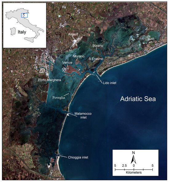
The Venice lagoon is located along the north-western coastline of the Adriatic Sea (45.10–45.35N, 12.10–12.40E) (Figure 1). It is the largest coastal lagoon in the Mediterranean region [42], covering an area of 550 km2 [6]. The main morphological features include intertidal and submerged mudflats, salt marshes, channels, creeks, islands, and extensive aquaculture—locally called “valli da pesca” [43]. The shallow water tidal flats of the lagoon average less than 1 m in depth and connect to the Adriatic Sea through three inlets: Lido, Malamocco, and Chioggia (Figure 1) [44,45]. The maximum depth of the lagoons’ tidal channels is around 15 m [46].
Figure 1.
Study area: The Venice lagoon from Sentinel-2 (19 December 2023).
The Venice lagoon experiences semidiurnal tides, featuring two high and two low tides daily. The height of the neap tide is 30 cm, the mean tide is 55 cm, and the spring tide is 110 cm [47]. The monthly average temperature is 14 °C, and the summer months from June to August are typically hot and humid. The average temperature during summer is 23 °C, while the highest recorded temperature can reach 35 °C. The monthly average rainfall is 70 mm, with the highest in September and October (98–104 mm) and the lowest from January to March (42–49 mm) [42].
The lagoon surrounds the historic city of Venice and other attractive tourist places (e.g., Burano, Murano, Lido, etc.) (Figure 1). The peculiar landscape of Venice city and its lagoon plays a crucial role in serving provisioning (e.g., fish and clam production), regulating (e.g., flood protection and carbon accumulation), and cultural ecosystem services (e.g., recreation and tourism). People living in the coastal area of the Venice region—as well as tourists from all over the world—directly or indirectly enjoy these ecosystem services for their livelihood. Recognizing distinctive and outstanding cultural, environmental, historic, artistic, and landscape values, UNESCO listed Venice and its lagoon as a World Cultural and Natural Heritage Site in 1987 [48].
3. Materials and Methods
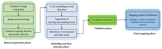
Our study utilized multiple images for weekends and weekdays across the summer and winter seasons from 2023 to 2025. To ensure the best accuracy, we designed a data processing procedure (Figure 2), which includes (i) Sentinel-2 image acquisition, (ii) image pre-processing, (iii) generate training datasets, (iv) U-Net modelling, (v) boat detection (including moving and standing boats), (vi) separation of moving (i.e., those transporting people or materials along the canals) and standing boats (i.e., those of people enjoying recreation in the most attractive areas of the lagoon), (vii) detection of recreational and regular transportation boats, (viii) accuracy assessment, and (ix) mapping spatial distribution.
Figure 2.
Boat detection and spatial distribution workflow.
3.1. Sentinel-2 Data Acquisition
This study employed Sentinel-2 Level-2A imagery at 10 m spatial resolution for visible bands, offering detailed optical data well suited for object detection in shallow coastal environments [49]. The orbital period is ten days, with a revisit period of two or three days in Europe and almost daily in the Arctic [30]. Sentinel-2 captures images of the Venice lagoon areas at around 10:05 a.m., a suitable time for detecting recreational boats and for mapping transportation along the canals.
Given the research question aimed at analyzing spatial patterns of recreational use, distinct from other uses of the lagoon (mainly for transportation), images were classified into separate groups, upon the observation that recreation activities are concentrated in weekends of the warmer months. Two seasons were identified: “summer”, i.e., the good season for recreation activities (June to September), and “winter”, i.e., the rest of the year. Moreover, separate analyses were conducted within the set of “summer” images for weekends (Saturday to Sunday) and weekdays (Monday to Friday). A total of 22 cloud-free images were collected from 2023 to 2025: 11 images for “summer” periods and 11 for “winter”; within the summer images, 6 cover weekdays and 5 weekends (see Table 1).
Table 1.
Sentinel-2 image acquisition.
Sentinel-2 images were retrieved using the OpenEO API [50] of the Copernicus Data Space Ecosystem. The download process was automated using a custom Python script that defined the spatial extent—specifically a bounding box encompassing the lagoon—while also filtering acquisitions based on date and cloud cover.
3.2. Image Pre-Processing
Due to limitations on download size, multiple tiles were retrieved and combined into a seamless raster using Rasterio 1.4.4 [50]. After that, the study area was extracted by considering the physical boundary of the Venice lagoon. A spatial mask with land areas was applied to restrict the analysis to aquatic surfaces. These pre-processing steps ensured that only open water areas were analyzed for boat detection.
3.3. Generation of Training Datasets and Model Selection
The boat detection workflow started by creating training datasets and verifying the distribution of boats across Sentinel-2 images. This preliminary analysis was necessary to support both the rule-based RGB thresholding approach and the subsequent deep learning segmentation stage [51], and to ensure that training data covered a wide range of optical and environmental conditions in the Venice lagoon.
In a first step, boat detection was performed using pixel-level filtering based on spectral reflectance properties. Training samples for the thresholding stage were manually annotated by identifying known boat locations on selected clipped scenes. The reflectance statistics of the annotated pixels were used to define empirical thresholds for each RGB band, corresponding to the 1st and 99th percentile reflectance values, with additional minimum and maximum caps to limit outliers. Each pixel was evaluated based on two criteria: (i) absolute reflectance thresholds and (ii) relative brightness compared to its local 3 × 3 and 5 × 5 pixel neighbourhoods. Pixels exceeding 15–20% of the neighbourhood mean brightness were retained as candidates. Boat candidate pixels were subsequently clustered using connected-component labelling, and for each cluster, the brightest pixel was selected as the representative detection point. This helped minimize over-counting in cases where multiple bright pixels belonged to the same vessel. As shown later, this approach was highly effective in open water areas where boats were spatially separated and spectral contrast between hulls and surrounding water was high.
However, in the Venice lagoon, boats are often tightly packed, or spectrally blended with urban infrastructure or shallow, muddy waters. Under such conditions, the limitations of pure pixel-based methods became evident, leading to missed detections and ambiguities in shallower water and mooring zones. To overcome these limitations, we complemented the RGB thresholding with a convolutional neural network (CNN) for semantic segmentation based on the U-Net architecture [52,53].
For the deep learning stage, training data consisted of cropped patches extracted from Sentinel-2 scenes, each resized to 256 × 256 pixels to match the model input. Patches were selected to cover a variety of situations, including: (i) isolated boats in open water, (ii) shallower waters and moorings, and (iii) spectrally challenging zones affected by turbidity or urban structures. Corresponding binary masks were manually digitized by two trained operators using Esri ArcGIS Pro 3.5, with boat footprints delineated at the pixel level. To ensure annotation reliability, cross-validation was performed: the two operators independently annotated 20% of the patches, achieving a Cohen’s Kappa intercoder reliability score of 0.87, indicating strong agreement [34].
The dataset was then split into three subsets: 70% for training, 15% for validation, and 15% as an independent test set that was not used during model development. The training set was used to fit the network parameters; the validation set was used for hyper-parameter tuning and early stopping; and the held-out test set was used to verify final accuracy.
The full detection pipeline, including RGB thresholding, U-Net segmentation, and subsequent moving or standing classification was implemented in Python 3.13.5 using PyCharm 2024.2 Professional Edition as the integrated development environment (IDE). All geospatial operations were carried out with open-source libraries, while the deep learning models were implemented in TensorFlow and run on GPU-accelerated hardware.
3.4. U-Net Modelling
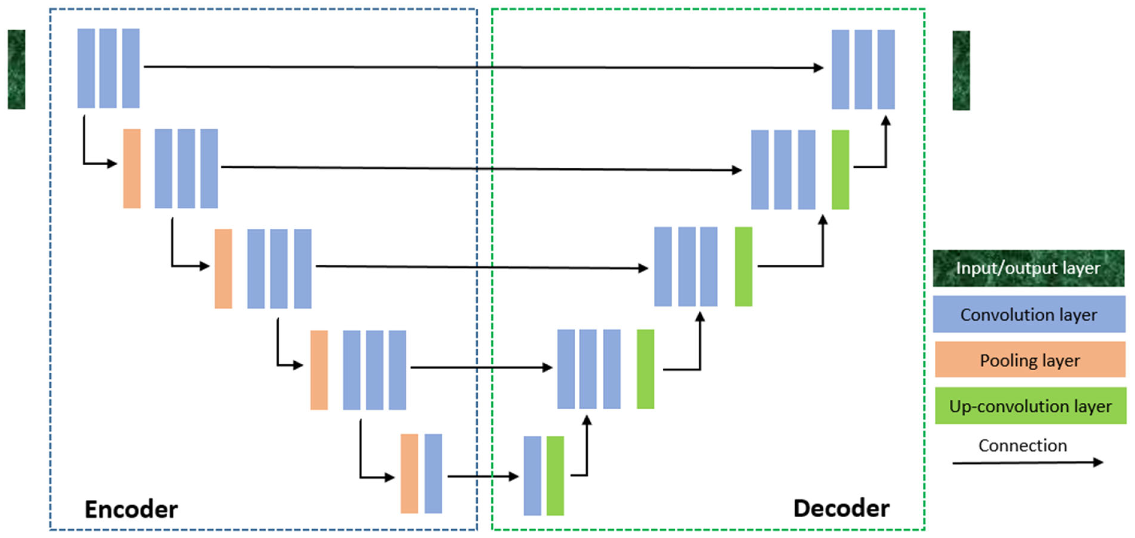
U-Net is characterized by a U-shaped architecture that consists of an encoder–decoder neural network featuring skip connections (Figure 3) that help preserve spatial information and enhance gradient flow during training [54]. The encoder consists of multiple convolutional layers that down-sample the image to extract relevant information. The encoder processes the input image and extracts features using multiple stacks of convolutional layers with pooling operations, such as max pooling. These pooling operations reduce the spatial resolution of the image while preserving higher-level features. Typically, each layer increases the number of filters, allowing for the learning of more complex features [53]. The encoder activation functions utilized are Sigmoid (σ) and then rectified linear units (f) due to their computational efficiency, faster convergence, and ability to mitigate vanishing gradient issues [37]. The σ and f functions correspond to Equations (1) and (2), respectively. The decoder section employs up-convolution layers to restore image resolution, and it merges encoder details with the decoder’s high-level features using concatenation. It culminates with a final convolutional layer that contains multiple filters corresponding to the predefined number of segmentation classes [41]. This layer acts as a classifier, producing a probability map as its output. Each pixel value in this map represents the probability that a specific pixel belongs to a particular class [53,55].
Figure 3.
The U-Net architecture functions as an encoder–decoder network. It features a contracting path on the left side, known as the encoder, which reduces the height and width of the input images while simultaneously increasing the depth through the use of convolutional and pooling layers. On the right side, the expansive path, referred to as the decoder, restores the original dimensions of the input images using up-sampling and convolutional layers.
The pooling layer plays a crucial role in reducing irrelevant parameters of the feature matrix and computation in the network. It commonly employs max pooling to down-sample the feature map. Max pooling is used strategically to retain important information related to the presence of objects (e.g., ships, boats, and other vessels) while gradually reducing the resolution of the feature map. This process is essential to the overall function of U-Net, as it improves the model’s ability to identify meaningful patterns and features in satellite imagery [37,56], ultimately leading to more accurate boat detection results, corresponding to Equation (3).
For the semantic segmentation of small recreational boats, we used a U-Net architecture in which the encoder was a ResNet-34 backbone pre-trained on ImageNet, while the decoder was initialized with random weights and trained from scratch [57]. This configuration preserves the U-shaped encoder–decoder structure while leveraging a more expressive feature extractor trained on a large natural image corpus. Only the encoder weights were pre-trained; the complete U-Net was fine-tuned end-to-end on our manually annotated Sentinel-2 dataset as described in the previous section. Unlike advanced variants such as Graph U-Net (which incorporates graph structures for relational reasoning) or other complex models (e.g., those using doubly stochastic graphs or tensor approximations), our standard U-Net with ResNet-34 offers simplicity, efficiency, and strong performance for pixel-level segmentation in remote sensing, particularly when combined with thresholding to handle Venice’s unique challenges. This sequential pipeline (thresholding for initial candidates + U-Net for refinement) is innovative for medium-resolution data in high-traffic lagoons, outperforming standalone methods in prior works (e.g., [32,34]) by reducing false positives from spectral blending.
Input patches were 256 × 256 pixels in RGB, normalized per band by the 1st–99th percentile stretch to reduce the influence of outliers and radiometric differences between scenes. Data augmentation included random horizontal/vertical flips, rotations (±15°), and mild brightness and contrast jitter, which is important for improving generalization under varying viewing and illumination conditions.
The network was trained using binary cross-entropy loss and the Adam optimizer with an initial learning rate of 1 × 10⁻⁴, batch size = 16, and a maximum of 50 epochs. An early-stopping strategy based on validation loss was applied, with a patience of 10 epochs, and the best model (with the lowest validation loss) was retained for subsequent inference. The train/validation/test split described in Section 3.3 (70/15/15) was strictly enforced: the test set was never used for architecture tuning or training and was only used once for final accuracy assessment.
By combining an ImageNet-pretrained ResNet-34 encoder with a U-Net decoder, our model benefits from both transfer learning and fine-grained segmentation capability, which has been shown to be effective for small-object detection in remote sensing [32]. In the context of the Venice lagoon, this configuration proved particularly useful to overcome the limitations of the RGB thresholding method. While direct comparisons with other models (e.g., Faster R-CNN or YOLO) were not conducted due to the unique dataset (high-density small boats in turbid waters), prior studies using such models on high-resolution data for larger vessels or low-traffic freshwater environments [34,36] report lower suitability for Sentinel-2 in complex lagoons, justifying our tailored approach.
3.5. Moving and Standing Boats
Each boat detection was labelled as either Standing (S) or Moving (M) through an analysis of the reflectance patterns and textural structures surrounding the boat in Sentinel-2 imagery. The method relies on the presence and morphology of surface wakes and is implemented through a probabilistic, radiometrically adaptive algorithm written in Python. The procedure integrates (i) local water radiometry, (ii) multi-directional wake evidence, (iii) fading-behaviour constraints, and (iv) morphological heuristics adapted to the 10 m spatial resolution of Sentinel-2 MSI [49].
3.5.1. Input Boat Points
For each detected boat point, a 19 × 19 pixel window (R = 9, approximately 190 m × 190 m) was extracted from the Sentinel-2 image to analyze the surrounding wake structure. The grayscale intensity image I(x,y) was computed by emphasizing the green and blue bands for distinguishing bright wakes against darker water backgrounds, corresponding to Equation (4), where each band was normalized using the 1st–99th percentile stretch. A Gaussian filter σ = 0.6 was used in scenes with high contrast, while σ = 0.8 was applied in more noisy areas to reduce false wake traces [49,58,59]. These values were selected empirically through visual evaluation of wake across multiple Sentinel-2 scenes.
A local water background was computed from an annular buffer (radius ≈ R − 3 px, thickness ≈ 2 px). This ring represents water near the boat but not influenced by the hull or wake. The upper 15% of pixel values was clipped to remove features, such as sun glints, piers and reflections [60]. The median of the remaining values defined the background level mi, while the median absolute deviation (MAD) provided a local dispersion estimate of the variability of the water brightness. To express this dispersion on a scale comparable to the standard deviation, the MAD was multiplied by 1.4826 (Equation (5)), yielding a robust standard deviation estimate [61]. These quantities guided both wake-detection thresholds and the classification of the moored vessels.
3.5.2. Boat Head Segmentation
The boat core was segmented using a dual-threshold procedure combining: (i) the local 80th-percentile brightness, which captures the top 20% of intensities within the window, and (ii) the Otsu adaptive threshold, computed from the local histogram [62]. The segmentation threshold was defined using Equation (6), ensuring that only the brightest, clearly distinguishable pixels were retained [63,64].
Small features (<1 px) were removed and a morphological opening (radius = 1 px) suppressed noise-like artefacts [65]. The brightest pixel in was selected as the boat head , representing the origin of potential wake development.
Two features were recorded: (i) core area (px), that represents the number of pixels in the boat, and (ii) core–background contrast , which is the difference between the mean intensity of the pixels representing the boats and the median intensity of the pixels of the surrounding water. The first feature is computed to support the identification of small standing boats [66,67,68,69] while the second feature helps to differentiate between the bright moving boats and the static ones with low contrast [70,71].
3.5.3. Wake Scan
The wake scan is a directional analysis designed to identify the wakes around a boat. Starting from the estimated boat head location, the algorithm analyzes the surrounding pixels along multiple radial directions to detect sequences of pixels whose brightness exceeds the local water background [69]. This procedure allows the identification of wake length, direction, contrast, and fading behaviour, which are key indicators of boat motion in medium-resolution optical imagery [70,71].
From , 36 rays (10° increments) were projected. Along each ray , contiguous pixels exceeding were counted, with .
Where Is = the brightness of a pixel at step s along the ray, = the local background median brightness (typical water level), = the robust standard deviation of water brightness around the boat (computed earlier), = a scaling constant (≈0.8, empirically calculated to exclude ripples and glints and include wakes with low contrast) [72,73,74], and = an absolute minimum threshold to hand low-contrast water. Consequently, the wake-detection threshold τ is the largest of an absolute contrast baseline (3% brightness above background), and a data-driven adaptive threshold proportional to the local variability (0.8 × σᵢ).
The algorithm then counts how many consecutive pixels along that ray have brightness greater than . Those consecutive bright pixels define the length of the wake in that direction.
Brightness was required to show a non-increasing trend, with any increase between consecutive steps not exceeding 25%, and each run’s average excess above background had to exceed 0.040, meaning a contrast above 3.5% brighter than the surrounding water [72]. The Spearman rank correlation coefficient () between pixel distance from the boat head and brightness intensity was computed to quantify the reduction in intensity along each potential wake [75].
A valid wake was required to exhibit a non-increasing trend, corresponding to , consistent with the expected fading of brightness with distance. This prevents false positives caused by distant bright spots (like sun-glint areas) that could make the brightness increase by moving away from the boat.
The two longest runs were compared to ensure directional uniqueness, requiring and verifying that there is a clear prevalent direction [76,77,78]. The longest validated run and its azimuth defined the candidate wake.
3.5.4. Classification of Moving and Standing Boats
For classifying the moving and standing boats, each boat was labelled using a three levels rule: Moving (M) if a confirmed wake existed with (and all fading/uniqueness checks passed) or regardless of secondary conditions [72,73].
In the first case the algorithm classifies the boat as standing if all the following conditions are met: smooth fading (≤25% increase rule), decreasing trend (), distinct direction (), sufficient brightness contrast (), the wake is at least 3 pixels long (≈30 m at 10 m/pixel). If the wake is very long (≥5 pixels ≈ 50 m), the boat is classified as moving if the other conditions are not met, to include some potential slow-moving objects that could not be identified according to the first rule [69,73,79].
Standing (S): otherwise, provided that , , , and , Cᵢ is the number of pixels in the segmented boat. The threshold was set by considering the spatial resolution of Sentinel-2 images: Sentinel-2 pixel = 10 m × 10 m = 100 m2. 9 px ≈ 900 m2 footprint that could be considered clearly exceeding the upper limit of a small recreational boat [58,59,68].
If Δᵢ ≤ 0.12, it means the boat is only about 12% brighter than its water background, which is typical of pale, stationary boats [66,67,80].
If (~20 m), there is no significant wake pattern, but only a compact or symmetric shape, typically indicating stationary or very slow-moving boats.
is the mean brightness of the “best” wake direction above the local water background. If it is ≤ 0.045, the pixels around the boat are only 4.5% brighter than the background, which is too faint for a true wake [72,79].
This rule preserved sensitivity to weak but elongated wakes while protecting small pale detections typical of moored or almost standing boats. These values support reproducibility and facilitate post-classification inspection in GIS software such as ArcGIS Pro. All images were processed automatically using a Python batch driver, matching each detection shapefile to its Sentinel-2 raster.
We explored the sensitivity of results to key parameters on selected images. For the crucial parameter of wake length threshold, we conducted an analysis using a subset of 150 boats from winter imagery, with an average wake length of around 4 pixels, consistent with typical wake characteristics at 10 m resolution. We tested classification thresholds ranging from 2 to 5 pixels under a simplified decision rule (a boat is classified as “moving” if wake length ≥ threshold).
The results (Table 2) show how increasing the threshold from the baseline value of 3 pixels decreased the number of boats classified as moving: a 28% reduction (from 120 to 86) at 4 pixels and a 55% reduction (to 54) at 5 pixels. Conversely, lowering the threshold to 2 pixels increased moving detections by 11% (to 133). These results are consistent with the visual inspection of additional image subsets, where higher thresholds reduced false positives for slow-moving boats, thus confirming the value chosen for that parameter.
Table 2.
Sensitivity of wake length threshold on boat classification.
3.6. Accuracy Assessment
Before mapping spatial indexes, the model performance was assessed through visual validation, because exhaustive ground-truth annotations were not available for the full study area. Ten image patches were randomly selected from the test dataset, containing approximately 500 boats in total. Detected boats were visually compared against human interpretations of the Sentinel-2 imagery.
Overall, the model correctly identified more than 90% of visually observable boats. Detection performance was strongly dependent on boat size. Larger boats (>10 m) were detected with high reliability, achieving an estimated detection rate of approximately 95%. In contrast, smaller boats (<10 m) were more frequently missed. These findings are consistent with previous Sentinel-2–based boat detection studies, which report a systematic reduction in detection accuracy for small targets and in optically complex waters such as lagoons and estuaries [32].
3.7. Mapping Spatial Indexes
Layers with points identifying boats (value = 1) were combined into maps for calculating two concise spatial indexes describing the spatial patterns of the two water uses of interest: the Water Recreation Index (WRI)—representing the density of standing boats—and the Water Transportation Index (WTI)—identifying the density of moving boats. We created spatial distribution maps of WRI and WTI ranging from 0 (no boats detected) to 1 (areas where boat were detected) using Ordinary Kriging (OK) in the Geostatistical Analyst toolbar in ArcGIS Pro. The OK method was chosen because it is widely used in the literature [81,82,83] and is frequently used to interpolate data in different aquatic environments [84,85], which provides higher accuracy than other interpolation methods [86,87,88]. During the OK interpolation process, the semivariograms were adapted to the spatial distributions of the various index maps by inputting the correct sill, range, lag, and nugget values [86].
4. Results
4.1. Spatio-Temporal Distribution of Boats in “Summer” and “Winter” Periods (2023–2025)
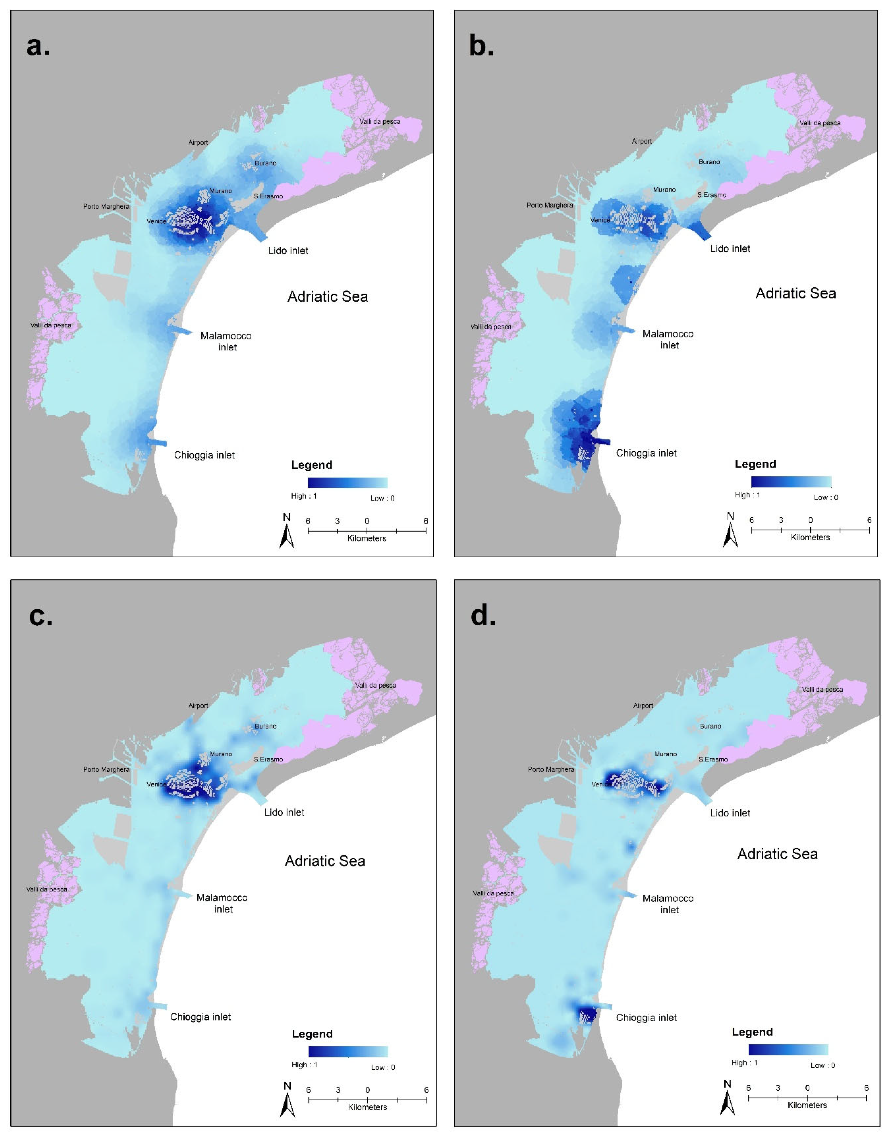
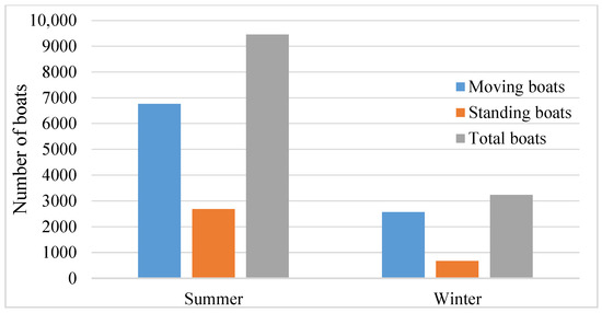
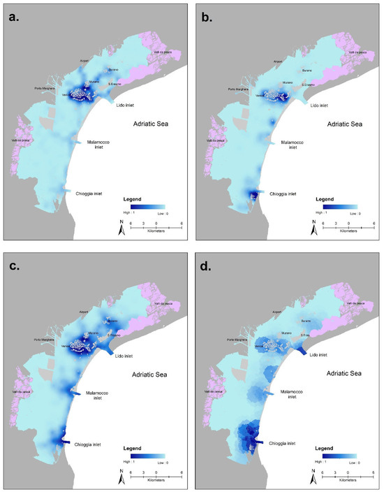
This study identifies statistically significant differences in the distribution of moving and standing boats across spatial (Figure 4) and temporal (Figure 5) scales during summer and winter.
Figure 4.
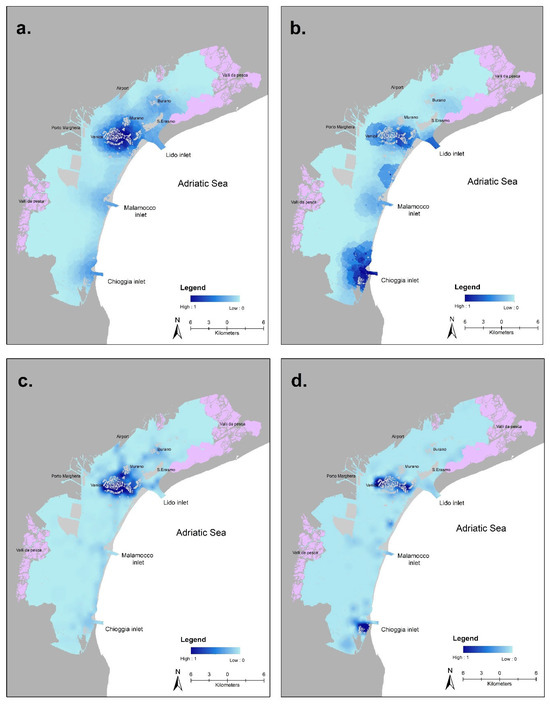
Spatial distribution of (a) WTI and (b) WRI during “summer”, and of (c) WTI and (d) WRI during “winter”.
Figure 5.
Temporal distribution of moving, standing, and total boats during summer and winter.
The spatial distribution maps of both moving and standing boats (WTI and WRI, respectively) was significantly higher in “summer” compared to “winter” (Figure 4). During summer, the boats were not only distributed around the islands of Venice, Murano, Burano, and San Erasmo, but also in other parts of the lagoon, including Lido, Malamocco, and Chioggia (Figure 4a,b). During “winter”, boats were primarily concentrated around the historical centre of Venice and along transportation routes following the main canals towards the airport and the islands Murano, Burano, etc. (Figure 4c,d).
The findings of our study demonstrate that the presence of standing boats is much higher and widespread in “summer” than in “winter” (Figure 4b,d, compared to Figure 4c,d) and it is distributed not only around the main islands but also in other parts of the lagoon (Figure 4b), thus indicating the areas of higher recreational attractiveness. These are, in particular, in the southern part of the lagoon, the three inlets, water surfaces around the city, and a spot in the central lagoon, where the small, abandoned island of Poveglia is located.
The findings of the temporal distribution indicate that the number of boats was significantly higher in the summer. Specifically, the moving and standing boats were two and four times higher, respectively, during summer compared to winter (Figure 5).
4.2. Spatio-Temporal Distribution of Boats in Weekdays and Weekends in Summer (2023–2025)
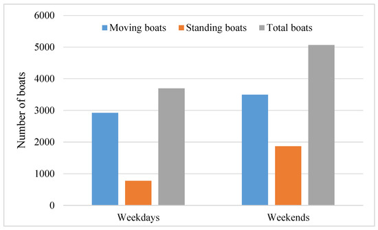
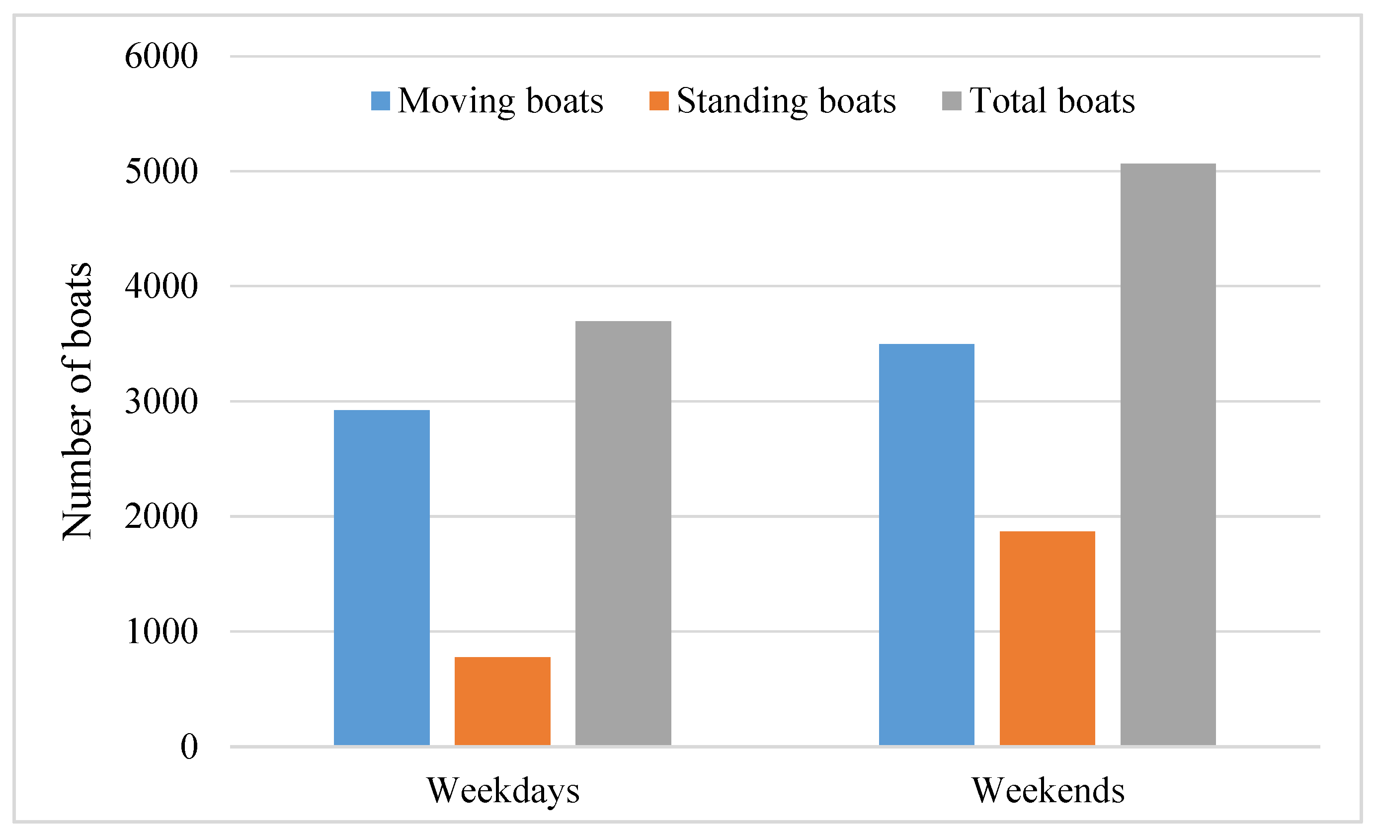
The study demonstrates a significant difference in the spatial (Figure 6) and temporal (Figure 7) distribution of moving and standing boats between summer weekdays and weekends.
Figure 6.
Spatial distribution of (a) WTI and (b) WRI during weekdays, and of (c) WTI and (d) WRI during weekends in “summer”.
Figure 7.
Temporal distribution of moving, standing, and total boats during summer weekdays and weekends.
The WTI is remarkably higher on summer weekends compared to weekdays. During summer weekdays, high values of WTI are concentrated only around Venice, while relatively low index values follow the main canals across the whole lagoon and towards the three inlets (Figure 6a). In contrast, on weekends, running boats clearly mark all the main canals and show very high values of the WTI in the areas around Venice, Murano, Burano and those close to the lagoon inlets (Figure 6c).
The concentration of standing boats was lower in the summer weekdays (Figure 6b) than on weekends (Figure 6d). On summer weekdays, the majority of these boats were found primarily in Venice and Chioggia, with other areas seeing much less activity; based on empirical observations, those areas coincide with those most attractive for amatorial fishing (Figure 6b). On weekends, as expected, the standing boats are more widely distributed, appearing not only around Venice but also at various lagoon locations; first of all the southern area close to Chioggia and the nearby inlet, but also the other two inlets and again the area around the island of Poveglia in the central lagoon (Figure 6d).
The findings of the temporal distribution indicate that the number of standing boats was more than twice as high during summer weekends compared to weekdays (Figure 7).
5. Discussion and Conclusions
Millions of tourists visit the historical city of Venice and its lagoon each year. Boats are the only means of transportation for locals and visitors, essential for navigating the city’s intricate network of canals experiencing its rich cultural heritage and for exploring the beautiful landscapes of the lagoon. The Vence Lagoon hosts various activities, ranging from the movement of people to the transportation of goods and the collection of garbage. Citizens and tourists use different types of boats, including vaporetto—a public transport service, gondola—a traditional rowing boat, traghetto—a ferry, water taxi—a quick transport, and a multitude of small private boats. According to Rova et al. [89], there are nearly 400,000 leisure boat trips used for recreation. The heavy boat traffic, along with the pollutants and noise it generates, negatively affects the movement, feeding, reproductive, and territorial behaviours of the lagoon’s biodiversity.
The detection of boats by means of remote sensing is then of crucial importance for safeguarding the main functions of the social-ecological system and planning for its sustainability.
This study explored the potential of applying rather innovative methods based on deep learning techniques to Sentinel-2 images, which offer very good opportunities in terms of availability and ease of use for free, but at the cost of relatively coarse resolution (10 m) for our purposes. We calculated and mapped two concise spatial indexes (WRI and WTI) to assess the spatial distribution of standing and moving boats across different seasons and days of the week in the Venice lagoon. Results show significant seasonal and weekly variations in the distribution of both running and standing boats within the Venice lagoon. Boat activity increases in the “summer” months, particularly on weekends, with clearly identified target areas of high attractiveness in various parts of the lagoon. In contrast, during the “winter” season, boats are detected mainly along the main canals used for various transportation purposes.
Results meet the expected pattern based on empirical observations, thus showing that the suboptimal resolution can be, at least in part, compensated by the innovative AI techniques and provide a quantitative basis for comparing recreational uses to generic boat transportation. The multi-year (2023–2025) analysis adds temporal depth, with the potential for extension to longer periods for trend analysis.
The findings of this study on the seasonal and weekly distribution of boats may assist in managing traffic to control wave-induced erosion and pollution by identifying areas heavily impacted by boat activity. Moreover, the present study might provide valuable insights into the spatial distribution of recreational boating hotspots and their environmental, but also economic relevance. This information could help in planning sustainable water-based tourism in the Venice lagoon and contribute to achieving the UN Sustainable Development Goals (SDGs), SDG 3, 6, 11, and 12, in particular.
The approach has limitations tied to data characteristics, such as the 10 m resolution limit and sub-pixel boat detection in turbid waters, as well as architecture (empirical parameters may vary by environment) and scenarios, particularly poor performance in complex cases like intersecting wakes or high winds and cloudy images, which reduce usability. Acquiring a comparable set of high-resolution images over three years would necessitate a significant financial investment. Moreover, accurate ground-truthing would be difficult to imagine for moving objects such as boats.
Empirical parameters in the wake classification algorithm were calibrated through visual assessment of sample images and a sensitivity analysis of the most important parameters was carried out. Overall, the results can be intended as a science-based contribution to the debate about the preservation and valorisation of the Venice Lagoon. Technical limitations are evident, as pointed out in the above text, but the novel contributions to the study of how recreational ecosystem services are used and their potential relevance for policy-making are also evident.
We hope that this work can raise the interest of decision- and policy-makers on the potential of remote sensing for the sustainable management of the Venice Lagoon and propitiate new resources for campaigns for the acquisition of high-resolution imagery from commercial satellites and for activities of ground-truthing, field validation, and consolidation of parameters for the specific characteristics of the environment. Future work could include comparisons with models like YOLO on adapted datasets and long-term analysis of the effects of climate and socio-economic trends on the supply and demand of recreational ecosystem services.
Author Contributions
A.H.K.: analysis of the literature, methodology, contribution to data processing, and paper writing; M.V.: methodology, data processing design and implementation, and paper writing; C.G.: conceptualization and coordination of the research and paper revision. All authors have read and agreed to the published version of the manuscript.
Funding
This work was supported by the Fondazione Eni Enrico Mattei (FEEM), Climate Change Adaptation Programme, Venice, Italy.
Data Availability Statement
Sentinel-2 data are available for free download from the Copernicus Data Space Ecosystem platform. Further inquiries can be directed to the corresponding author.
Acknowledgments
We thank the anonymous reviewers and editor for their insightful comments and suggestions. We wish to extend our thanks to the Climate Change Adaptation at FEEM in Venice, Italy.
Conflicts of Interest
The authors declare no conflicts of interest relating to publishing of this paper.
References
- ST/ESA/STAT/SER.M/88; Manual for the National Standardization of Geographical Names. UNSD (The United Nations Statistics Division), United Nations: New York, NY, USA, 2006. Available online: http://unstats.un.org/unsd/geoinfo/ (accessed on 22 April 2025).
- Shalby, A.; Elshemy, M.; Zeidan, B. Modeling of climate change impacts on Lake Burullus, coastal lagoon (Egypt). Int. J. Sediment Res. 2021, 36, 756–769. [Google Scholar] [CrossRef] [Scilit]
- Newton, A.; Icely, J.; Cristina, S.; Perillo, G.M.E.; Turner, R.E.; Ashan, D.; Cragg, S.; Luo, Y.; Tu, C.; Li, Y.; et al. Anthropogenic, Direct Pressures on Coastal Wetlands. Front. Ecol. Evol. 2020, 8, 2441001. [Google Scholar] [CrossRef] [Scilit]
- Inácio, M.; Barboza, F.R.; Villoslada, M. The protection of coastal lagoons as a nature-based solution to mitigate coastal floods. Curr. Opin. Env. Sci. Health 2023, 34, 100491. [Google Scholar] [CrossRef] [Scilit]
- Haines-Young, R.; Potschin, M. Common International Classification of Ecosystem Services (CICES) V5.1; Fabis: Nottingham, UK, 2018; Available online: https://cices.eu/content/uploads/sites/8/2018/01/Guidance-V51-01012018.pdf (accessed on 28 April 2025).
- Newton, A.; Icely, J.; Cristina, S.; Brito, A.; Cardoso, A.C.; Colijn, F.; Riva, S.D.; Gertz, F.; Hansen, J.W.; Holmer, M.; et al. An overview of ecological status, vulnerability and future perspectives of European large shallow, semi-enclosed coastal systems, lagoons and transitional waters. Estua. Coast. Shelf Sci. 2014, 140, 95–122. [Google Scholar] [CrossRef] [Scilit]
- Lassere, P. Coastal Lagoons: Sanctuary Ecosystems, Cradles of Culture, Targets for Economic Growth; UNESCO: Paris, France, 1979; pp. 2–21. Available online: https://unesdoc.unesco.org/ark:/48223/pf0000061589 (accessed on 30 April 2025).
- Gössling, S.; Hall, C.M.; Scott, D. Tourism and Water; Channel View Publications; Blue Ridge Summit: Bristol, UK, 2015. [Google Scholar]
- Orams, M. Marine Tourism: Development, Impacts and Management; Routledge: London, UK, 1999. [Google Scholar]
- Jennings, G. Water-Based Tourism, Sport, Leisure, and Recreation Experiences; Routledge: London, UK, 2007. [Google Scholar]
- Tuohino, A. The potential of lakes and lake landscape in the concept of nordic wellbeing. Pol. J. Nat. Sci. 2013, 28, 267–281. [Google Scholar]
- Furgała-Selezniow, G.; Jankun-Wo’znicka, M.; Kruk, M.; Omelan, A.A. Land Use and Land Cover Pattern as a Measure of Tourism Impact on a Lakeshore Zone. Land 2021, 10, 787. [Google Scholar] [CrossRef] [Scilit]
- Mitra, S.K. Is tourism-led growth hypothesis still valid? Int. J. Tour. Res. 2019, 21, 615–624. [Google Scholar] [CrossRef] [Scilit]
- Drius, M.; Bongiorni, L.; Depellegrin, D.; Menegon, S.; Pugnetti, A.; Stifter, S. Tackling challenges for Mediterranean sustainable coastal tourism: An ecosystem service perspective. Sci. Total Environ. 2019, 652, 1302–1317. [Google Scholar] [CrossRef] [Scilit]
- Stocco, A.; Pranovi, F. The paradoxical need for human intervention in the conservation of natural environments in Venice lagoon. Sci Rep. 2023, 13, 6798. [Google Scholar] [CrossRef] [Scilit]
- Choi, J.; Jeon, H.; Asperin, A. Popularity Paradox in Venice, Italy: A Battle of Priorities. J. Hosp. Tour. Cases 2024, 13, 159–168. [Google Scholar] [CrossRef] [Scilit]
- Giupponi, C.; Bidoia, M.; Breil, M.; Corato, L.D.; Gain, A.H.; Leoni, V.; Fard, B.M.; Pesenti, R.; Umgiesser, G. Boon and burden: Economic performance and future perspectives of the Venice flood protection system. Reg. Environ. Change 2024, 24, 44. [Google Scholar] [CrossRef] [Scilit]
- Anzidei, M.; Tolomei, C.; Trippanera, D.; Alberti, T.; Bosman, A.; Brunori, C.A.; Serpelloni, E.; Vecchio, A.; Falciano, A.; Deli, G. Multi-Temporal Relative Sea Level Rise Scenarios up to 2150 for the Venice Lagoon (Italy). Remote Sens. 2025, 17, 820. [Google Scholar] [CrossRef] [Scilit]
- Bolgan, M.; Picciulin, M.; Codarin, A.; Fiorin, R.; Zucchetta, M.; Malavasi, S. Is the Venice Lagoon Noisy? First Passive Listening Monitoring of the Venice Lagoon: Possible Effects on the Typical Fish Community. In The Effects of Noise on Aquatic Life II. Advances in Experimental Medicine and Biology; Popper, A., Hawkins, A., Eds.; Springer: New York, NY, USA, 2016; Volume 875. [Google Scholar] [CrossRef] [Scilit]
- Picciulin, M.; Zucchetta, M.; Facca, C.; Malavasi, S. Boat-induced pressure does not influence breeding site selection of a vulnerable fish species in a highly anthropized coastal area. Mar. Pollut. Bull. 2022, 180, 113750. [Google Scholar] [CrossRef] [Scilit] [PubMed]
- La Manna, G.; Manghi, M.; Perretti, F.; Sara, G. Behavioural response of brown meagre (Sciaena umbra) to boat noise. Mar. Pollut. Bull. 2016, 110, 324–334. [Google Scholar] [CrossRef] [Scilit]
- Bracciali, C.; Campobello, D.; Giacoma, C.; Sara, G. Effects of nautical traffic and noise on foraging patterns of Mediterranean damselfish (Chromis chromis). PLoS ONE 2012, 7, e40582. [Google Scholar] [CrossRef] [Scilit]
- Slabbekoorn, H.; Bouton, N.; Van Opzeeland, I.; Coers, A.; Ten Cate, C.M.; Popper, A.N. A Noisy Spring: The Impact of Globally Rising Underwater Sound Levels on Fish. Trends Ecol. Evol. 2010, 25, 419–427. [Google Scholar] [CrossRef] [Scilit]
- Cecchi, T.; Poletto, D. ‘Ghost Boats’ in Venice: Environmental concerns, green chemical fingerprint, circular and sustainable end-of-life-solutions. Sci. Total Environ. 2025, 973, 179126. [Google Scholar] [CrossRef] [Scilit]
- Tseng, Y.P.; Kyle, G.T.; Shafer, C.S.; Graefe, A.R.; Bradle, T.A.; Schuett, M.A. Exploring the Crowding–Satisfaction Relationship in Recreational Boating. Environ. Manag. 2009, 43, 496–507. [Google Scholar] [CrossRef] [Scilit]
- Jialeng, G.; Fuente, S.; Smith, T. BoatNet: Automated small boat composition detection using deep learning on satellite imagery. UCL Open Environ. 2023, 5, e058-20. [Google Scholar] [CrossRef] [Scilit]
- Jozdani, S.E.; Johnson, B.A.; Chen, D. Comparing deep neural networks, ensemble classifiers, and support vector machine algorithms for object-based urban land use/land cover classification. Remote Sens. 2019, 11, 1713. [Google Scholar] [CrossRef] [Scilit]
- Pourbabaee, B.; Roshtkhari, M.J.; Khorasani, K. Deep convolutional neural networks and learning ECG features for screening paroxysmal atrial fibrillation patients. IEEE Trans. Syst. Man Cybern. Syst. 2017, 48, 2095–2104. [Google Scholar] [CrossRef] [Scilit]
- Kumar, M.S.; Ganesh, D.; Turukmane, A.V.; Batta, U.; Sayyadliyakat, K.K. Deep convolution neural network based solution for detecting plant diseases. J. Pharm. Negat. Results 2022, 13, 464–471. [Google Scholar] [CrossRef] [Scilit]
- Heiselberg, P.; Heiselberg, H. Ship-Iceberg Discrimination in Sentinel-2 Multispectral Imagery by Supervised Classification. Remote Sens. 2017, 9, 1156. [Google Scholar] [CrossRef] [Scilit]
- Yin, Z.Y.; Tang, Y.Q.; Chen, Y.Z.; Zhang, Y.Y. A Ship Monitoring Framework Based on Multimodal Remote Sensing Data. J. Phys. Conf. Ser. 2023, 2486, 012018. [Google Scholar] [CrossRef] [Scilit]
- Ciocarlan, A.; Stoian, A. Ship Detection in Sentinel 2 Multi-Spectral Images with Self-Supervised Learning. Remote Sens. 2021, 13, 4255. [Google Scholar] [CrossRef] [Scilit]
- Wu, F.; Zhou, Z.; Wang, B.; Ma, J. Inshore Ship Detection Based on Convolutional Neural Network in Optical Satellite Images. IEEE J. Sel. Top. Appl. Earth Obs. Remote Sens. 2018, 11, 4005–4015. [Google Scholar] [CrossRef] [Scilit]
- Rucinski, M.; Wozniak, E.; Kulczyk, S.; Derek, M. Small Recreational Boat Detection Using Sentinel-1 Data for the Monitoring of Recreational Ecosystem Services. Remote Sens. 2023, 15, 1807. [Google Scholar] [CrossRef] [Scilit]
- Ghamisi, P.; Yokoya, N.; Li, J.; Liao, W.; Liu, S.; Plaza, J.; Rasti, B.; Plaza, A. Advances in hyperspectral image and signal processing: A comprehensive overview of the state of the art. IEEE Geosci. Remote Sens. Mag. 2018, 5, 37–78. [Google Scholar] [CrossRef] [Scilit]
- Gajjar, P.; Garg, M.; Shah, V.; Shah, P.; Das, A. Applicability analysis of attention U-Nets over vanilla variants for automated ship detection. Rep. Geod. Geoinform. 2022, 114, 9–14. [Google Scholar] [CrossRef] [Scilit]
- Niranjan, A.; Patial, S.; Aryan, A.; Mittal, A.; Choudhury, T.; Rabiei-Dastjerdi, H.; Kumar, P. A Deep Learning Approach for Ship Detection Using Satellite Imagery. EAI Endorsed Trans. Internet Things 2024, 10, 5435. [Google Scholar] [CrossRef] [Scilit]
- Shen, D.; Wu, G.; Suk, H.I. Deep learning in medical image analysis. Annu. Rev. Biomed. Eng. 2017, 19, 221–248. [Google Scholar] [CrossRef] [Scilit]
- Sherrah, J. Fully convolutional networks for dense semantic labelling of high-resolution aerial imagery. arXiv 2016, arXiv:1606.02585. [Google Scholar] [CrossRef] [Scilit]
- Kampffmeyer, M.; Salberg, A.B.; Jenssen, R. Semantic segmentation of small objects and modeling of uncertainty in urban remote sensing images using deep convolutional neural networks. In Proceedings of the 2016 IEEE Conference on Computer Vision and Pattern Recognition Workshops (CVPRW), Las Vegas, NV, USA, 26 June–1 July 2016. [Google Scholar] [CrossRef] [Scilit]
- Wu, N.; Jia, D.; Li, Z.; He, Z. Weak Edge Target Segmentation Network Based on Dual Attention Mechanism. Appl. Sci. 2024, 14, 8963. [Google Scholar] [CrossRef] [Scilit]
- Taramelli, A.; Valentini, E.; Piedelobo, L.; Righini, M.; Cappucci, S. Assessment of State Transition Dynamics of Coastal Wetlands in Northern Venice Lagoon, Italy. Sustainability 2021, 13, 4102. [Google Scholar] [CrossRef] [Scilit]
- Rova, S.; Pranovi, F.; Müller, F. Provision of ecosystem services in the lagoon of Venice (Italy): An initial spatial assessment. Ecohydrol. Hydrobiol. 2015, 15, 13–25. [Google Scholar] [CrossRef] [Scilit]
- Madricardo, F.; Donnici, S. Mapping past and recent landscape modifications in the Lagoon of Venice through geophysical surveys and historical maps. Anthropocene 2014, 6, 86–96. [Google Scholar] [CrossRef] [Scilit]
- Lasserre, P.; Marzollo, A. (Eds.) The Venice Lagoon Ecosystem: Inputs and Interactions Between Land and Sea; Series: Man and the Biosphere; Parthenon: Nashville, TN, USA, 2000; Volume 25, Available online: https://archive.org/details/venicelagoonecos0025unse (accessed on 30 April 2025).
- Ferrarin, C.; Bonaldo, D.; Bergamasco, A.; Ghezzo, M. Sea level and temperature extremes in a regulated Lagoon of Venice. Front. Clim. 2024, 5, 1330388. [Google Scholar] [CrossRef] [Scilit]
- Cappucci, S.; Amos, C.L.; Hosoe, T.; Umgiesser, G. SLIM: A numerical model to evaluate the factors controlling the evolution of intertidal mudflats in Venice Lagoon, Italy. J. Mar. Syst. 2004, 51, 257–280. [Google Scholar] [CrossRef] [Scilit]
- Lionello, P.; Nicholls, R.J.; Umgiesser, G.; Zanchettin, D. Venice flooding and sea level: Past evolution, present issues, and future projections (introduction to the special issue). Nat. Hazards Earth Syst. Sci. 2021, 21, 2633–2641. [Google Scholar] [CrossRef] [Scilit]
- Drusch, M.; Del Bello, U.; Carlier, S.; Colin, O.; Fernandez, V.; Gascon, F.; Hoersch, B.; Isola, C.; Laberinti, P.; Martimort, P.; et al. Sentinel-2: ESA’s Optical High-Resolution Mission for GMES Operational Services. Remote Sens. Environ. 2012, 120, 25–36. [Google Scholar] [CrossRef] [Scilit]
- Schramm, M.; Pebesma, E.; Milenković, M.; Foresta, L.; Dries, J.; Jacob, A.; Wagner, W.; Mohr, M.; Neteler, M.; Kadunc, M.; et al. The openEO API–Harmonising the Use of Earth Observation Cloud Services Using Virtual Data Cube Functionalities. Remote Sens. 2021, 13, 1125. [Google Scholar] [CrossRef] [Scilit]
- Hendrycks, D.; Lee, K.; Mazeika, M. Using pre-training can improve model robustness and uncertainty. arXiv 2019, arXiv:1901.09960. [Google Scholar] [CrossRef] [Scilit]
- Ronneberger, O.; Fischer, P.; Brox, T. U-Net: Convolutional Networks for Biomedical Image Segmentation. arXiv 2015, arXiv:1505.04597. [Google Scholar] [CrossRef] [Scilit]
- Dimitrovski, I.; Spasev, V.; Loshkovska, S.; Kitanovski, I. U-Net Ensemble for Enhanced Semantic Segmentation in Remote Sensing Imagery. Remote Sens. 2024, 16, 2077. [Google Scholar] [CrossRef] [Scilit]
- George, G.; Anusuya, S. Pretrained U-Net: In-depth analysis of binary image segmentation in underwater marine environment. Mach. Learn. Comput. Sci. Eng. 2025, 1, 4. [Google Scholar] [CrossRef] [Scilit]
- Jumutc, V.; Bliznuks, D.; Lihachev, A. Multi-Path U-Net Architecture for Cell and Colony-Forming Unit Image Segmentation. Sensors 2022, 22, 990. [Google Scholar] [CrossRef] [Scilit]
- Chhor, G.; Aramburu, C.B.; Bougdal-Lambert, I. Satellite Image Segmentation for Building Detection Using U-Net. 2017. Available online: http://cs229.stanford.edu/proj2017/final-reports/5243715.pdf (accessed on 18 June 2025).
- Cui, Z. AnAttention-Based Improved U-Net Neural Network Model for Semantic Segmentation of Moving Objects. IEEE Access 2024, 12, 57071–57081. [Google Scholar] [CrossRef] [Scilit]
- Pahlevan, N.; Sarkar, S.; Franz, B.A.; Balasubramanian, S.V.; He, J. Sentinel-2 MultiSpectral Instrument (MSI) data processing for aquatic science applications: Demonstrations and validations. Remote Sens. Environ. 2017, 201, 47–56. [Google Scholar] [CrossRef] [Scilit]
- Vanhellemont, Q.; Ruddick, K. Atmospheric correction of metre-scale optical satellite data for inland and coastal water applications. Remote Sens. Environ. 2018, 216, 586–597. [Google Scholar] [CrossRef] [Scilit]
- Vanhellemont, Q. Adaptation of the dark spectrum fitting atmospheric correction for aquatic applications of the Landsat and Sentinel-2 archives. Remote Sens. Environ. 2019, 225, 175–192. [Google Scholar] [CrossRef] [Scilit]
- Rousseeuw, P.J.; Croux, C. Alternatives to the median absolute deviation. J. Am. Stat. Assoc. 1993, 88, 1273–1283. [Google Scholar] [CrossRef]
- Otsu, N. Threshold Selection from Gray-Level Histograms. IEEE Trans. Syst. Man Cyber. 1979, 9, 62–66. [Google Scholar] [CrossRef] [Scilit]
- Bradley, D.; Roth, G. Adaptive thresholding using the integral image. J. Graph. Tools 2007, 12, 13–21. [Google Scholar] [CrossRef] [Scilit]
- Che, L.; Li, S.; Liu, X. Improved surface water mapping using satellite remote sensing imagery based on optimization of the Otsu threshold and effective selection of remote-sensing water index. J. Hydrol. 2025, 654, 132771. [Google Scholar] [CrossRef] [Scilit]
- Soille, P. Morphological Image Analysis: Principles and Applications; Springer: Berlin, Germany, 1999; Volume 2, pp. 170–217. Available online: https://link.springer.com/book/10.1007/978-3-662-05088-0 (accessed on 10 June 2025).
- Blaschke, T.; Hay, G.J.; Kelly, M.; Lang, S.; Hofmann, P.; Addink, E.; Feitosa, R.Q.; Meer, F.V.D.; Werff, H.V.D.; Coillie, F.V.; et al. Geographic Object-Based Image Analysis—Towards a new paradigm. ISPRS J. Photogramm. Remote Sens. 2014, 87, 180–191. [Google Scholar] [CrossRef] [Scilit]
- Ma, L.; Liu, Y.; Zhang, X.; Ye, Y.; Yin, G.; Johnson, B.A. Deep learning in remote sensing applications: A meta-analysis and review. ISPRS J. Photogramm. Remote Sens. 2019, 152, 166–177. [Google Scholar] [CrossRef] [Scilit]
- Qin, Y.; Bruzzone, L.; Gao, C.; Li, B. Infrared small target detection based on facet kernel and random walker. IEEE Trans. Geosci. Remote Sens. 2019, 57, 7104–7118. [Google Scholar] [CrossRef] [Scilit]
- Mazzeo, A.; Renga, A.; Graziano, M.D. A Systematic Review of Ship Wake Detection Methods in Satellite Imagery. Remote Sens. 2024, 16, 3775. [Google Scholar] [CrossRef] [Scilit]
- Liu, Y.; Zhao, J.; Qin, Y. A novel technique for ship wake detection from optical images. Remote Sens. Environ. 2021, 258, 112375. [Google Scholar] [CrossRef] [Scilit]
- Choi, S.; Jeon, W.; Jung, I.; Jung, D.; Sim, S.; Woo, J.; Kim, H.; Park, S.; Kim, S.; Lee, S.; et al. Integrated Detection of Ships and Their Wakes Using Sentinel-2A Imagery and Automated Machine Learning Approaches. Mar. Geod. 2025, 48, 665–687. [Google Scholar] [CrossRef] [Scilit]
- Li, H.; Yang, S.; Zhang, R.; Yu, P.; Fu, Z.; Wang, X.; Kadoch, M.; Yang, Y. Detection of Floating Objects on Water Surface Using YOLOv5s in an Edge Computing Environment. Water 2024, 16, 86. [Google Scholar] [CrossRef] [Scilit]
- Liu, Y.; Zhang, R.; Deng, R.; Zhao, J. Ship detection and classification based on cascaded detection of hull and wake from optical satellite remote sensing imagery. GIScience Remote Sens. 2023, 60, 2196159. [Google Scholar] [CrossRef] [Scilit]
- Li, L.; Zhou, Z.; Wang, B.; Miao, L.; An, Z.; Xiao, X. Domain Adaptive Ship Detection in Optical Remote Sensing Images. Remote Sens. 2021, 13, 3168. [Google Scholar] [CrossRef] [Scilit]
- Helsel, D.R.; Hirsch, R.M.; Ryberg, K.R.; Archfield, S.A.; Gilroy, E.J. Techniques and Methods. In Statistical Methods in Water Resources; Book 4, Chapter A3; U.S. Geological Survey: Reston, VA, USA, 2020; 458p. [Google Scholar] [CrossRef] [Scilit]
- Tsai, D.M.; Hsieh, C.Y. Automated surface inspection for directional textures. Image Vis. Comput. 1999, 18, 49–62. [Google Scholar] [CrossRef] [Scilit]
- Wang, G.; Zhang, X.; Zhu, P.; Tang, X.; Chen, P.; Jiao, L.; Zhou, H. High-quality angle prediction for oriented object detection in remote sensing images. IEEE Trans. Geosci. Remote Sens. 2023, 61, 5614714. [Google Scholar] [CrossRef] [Scilit]
- Scherbakov, A.; Hanssen, R.; Vosselman, G.; Feron, R. Ship wake detection using Radon transforms of filtered SAR imagery. In Microwave Sensing and Synthetic Aperture Radar, Proceedings of SPIE Satellite Remote Sensing, Taormina, Italy, 23–27 September 1996; SPIE: Bellingham, DC, USA, 1996. [Google Scholar] [CrossRef] [Scilit]
- Ermakov, S.; Kapustin, I.; Lazareva, T. Ship wake signatures in radar/optical images of the sea surface: Observations and physical mechanisms. In Remote Sensing of the Ocean, Sea Ice, Coastal Waters, and Large Water Regions, Proceedings of SPIE Remote Sensing, Amsterdam, The Netherlands, 22–25 September 2014; SPIE: Bellingham, DC, USA, 2014. [Google Scholar] [CrossRef] [Scilit]
- Li, Z.; Wang, Y.; Zhang, N.; Zhang, Y.; Zhao, Z.; Xu, D.; Ben, G.; Gao, Y. Deep Learning-Based Object Detection Techniques for Remote Sensing Images: A Survey. Remote Sens. 2022, 14, 2385. [Google Scholar] [CrossRef] [Scilit]
- Li, J.; Heap, A.D. A Review of Spatial Interpolation Methods for Environmental Scientists; Geoscience Australia: Canberra, Australia, 2008. [Google Scholar]
- Azpurua, M.; dos Ramos, K. A comparison of spatial interpolation methods for estimation of average electromagnetic field magnitude. Prog. Electromagn. Res. M 2010, 14, 135–145. [Google Scholar] [CrossRef] [Scilit]
- Meng, Q.; Liu, Z.; Borders, B.E. Assessment of regression kriging for Spatial interpolation—Comparisons of seven GIS interpolation methods. Cartogr. Geogr. Inf. Sci. 2013, 40, 28–39. [Google Scholar] [CrossRef] [Scilit]
- Merwade, V.M.; Maidment, D.R.; Goff, J.A. Anisotropic considerations while interpolating river channel bathymetry. J. Hydrol. 2006, 331, 731–741. [Google Scholar] [CrossRef] [Scilit]
- Bello-Pineda, J.; Stefanoni-Hernández, J.L. Comparing the performance of two spatial interpolation methods for creating a digital bathymetric model of the Yucatan submerged platform. Pan-Am. J. Aquat. Sci. 2007, 2, 247–254. [Google Scholar]
- Curtarelli, M.; Leão, J.; Ogashawara, I.; Lorenzzetti, J.; Stech, J. Assessment of Spatial Interpolation Methods to Map the Bathymetry of an Amazonian Hydroelectric Reservoir to Aid in Decision Making for Water Management. ISPRS Int. J. Geo-Inform. 2015, 4, 220–235. [Google Scholar] [CrossRef] [Scilit]
- Wu, C.Y.; Mossa, J.; Mao, L.; Almulla, M. Comparison of different spatial interpolation methods for historical hydrographic data of the lowermost Mississippi River. Ann. GIS 2019, 25, 133–151. [Google Scholar] [CrossRef] [Scilit]
- Boumpoulis, V.; Michalopoulou, M.; Depountis, N. Comparison between different spatial interpolation methods for the development of sediment distribution maps in coastal areas. Earth Sci. Inform. 2023, 16, 2069–2087. [Google Scholar] [CrossRef] [Scilit]
- Rova, S.; Stocco, A.; Pranovi, F. Ecosystem services’ capacity and flow in the Venice Lagoon and the relationship with ecological status. OneEcosystem 2022, 7, e79715. [Google Scholar] [CrossRef] [Scilit]

Disclaimer/Publisher’s Note: The statements, opinions and data contained in all publications are solely those of the individual author(s) and contributor(s) and not of MDPI and/or the editor(s). MDPI and/or the editor(s) disclaim responsibility for any injury to people or property resulting from any ideas, methods, instructions or products referred to in the content. |
© 2026 by the authors. Licensee MDPI, Basel, Switzerland. This article is an open access article distributed under the terms and conditions of the Creative Commons Attribution (CC BY) license.