


Highlights
What are the main findings?
- The proposed BCTBM architecture incorporating BCKE achieves superior seafloor sediment classification, with an average OA improvement of 3.48% and a maximum increment of 9.4%.
- The two-stage BM-mRMR feature selection integrates MIC and Bayesian optimization, outperforming ReliefF and ReliefF-mRMR by 4.84% and 6.08% in average accuracy, respectively.
What are the implications of the main findings?
- Incorporating bottom-current kinetic energy introduces physical prior information for sediment classification, and the classification results agree well with the Hjulström–Sundborg sedimentary-dynamic framework.
- The BCTBM framework provides a physically interpretable solution for refined seafloor sediment mapping and supports benthic habitat investigation in shelf sea regions.
Abstract
Seafloor sediment classification is critical for benthic habitat mapping and marine environmental protection. Existing classification methods mostly adopt seafloor surface observation parameters such as backscatter and bathymetry. These parameters only characterize surface seabed properties and lack physical prior information related to sediment formation mechanisms, which limits classification accuracy and physical interpretability. Considering that bottom-current kinetic energy (BCKE) governs sediment erosion, transport and deposition and further shapes the spatial distribution of sediments, this paper proposes a bottom-current-fused two-stage Bayesian MIC-augmented mRMR (BCTBM) architecture for seafloor sediment classification. BCTBM combines BCKE with acoustic and topographic features to construct a 77-dimensional multi-source feature set. Samples with high class separability are selected using the Jeffries–Matusita (J-M) distance, and a two-stage feature selection algorithm is further developed. ReliefF is first applied for coarse-grained feature screening to generate a candidate feature set; subsequently, the Bayesian MIC-augmented Minimum Redundancy Maximum Relevance (BM-mRMR) model employs Bayesian optimization (BO) to adaptively solve the optimal relevance–redundancy trade-off weights for seven target dimensions, and mRMR finally derives the optimal feature set based on the obtained optimal weights. The proposed method is validated in the shallow-water sediment classification scenario of the eastern English Channel. Eighty-four comparative experiments demonstrate that introducing BCKE improves the overall accuracy by 3.48% on average, with a maximum increment of 9.4%. The proposed two-stage BM-mRMR method achieves average accuracy improvements of 4.84% and 6.08% over ReliefF and ReliefF-mRMR, respectively. The classification results are consistent with the Hjulström–Sundborg sedimentary-dynamic framework, offering an effective pathway for refined benthic habitat mapping.
1. Introduction
Seafloor sediment is a fundamental component of the marine environment, and its type and spatial distribution are directly relevant to marine engineering, seabed resource exploration, ecological conservation, and underwater acoustic applications [1,2]. Accurate acquisition of sediment information is essential for understanding sedimentary dynamic processes, conducting benthic habitat mapping, and assessing marine environmental changes [3,4,5,6]. Acoustic remote sensing technologies, particularly multibeam echo sounders and side-scan sonars, have become the primary means for large-scale seafloor sediment surveys owing to their long detection range, strong environmental adaptability, and high detection efficiency [7,8,9]. By transmitting sound waves and receiving seafloor echoes, acoustic detection can rapidly acquire data such as backscatter intensity and water depth, which are closely related to physical properties including sediment grain composition, surface roughness, and compactness, thus providing reliable evidence for sediment type identification [10,11]. With continuous advances in surveying technology and data processing methods, acoustic-based sediment classification has developed into an important direction in marine geological research and engineering applications [12].
Traditional acoustic classification studies of seafloor sediments have largely relied on backscatter intensity or topographic features for classification [13,14,15]. Although these methods can realize basic classification, their classification results lack physical interpretability. Moreover, different sediment types may produce similar backscatter and topographic signals, leading to seafloor sediment misclassification. Backscatter intensity primarily reflects the microscopic roughness of the seafloor surface, while topographic data emphasize macroscopic geomorphology; both are static information sources and are insufficient to reveal the hydrodynamic genesis of sediment formation. With the rapid development of marine observation technologies, multi-source data including topography, backscatter, and bottom currents have become progressively accessible [16,17], offering new opportunities for fine-scale sediment classification. In fact, hydrodynamic conditions directly control the erosion, transport, and deposition of sediments, serving as the core driving force that determines the spatial distribution of sediment types: high-energy environments tend to scour fine particles, favoring the formation of coarse-grained deposits, whereas low-energy environments allow the preservation of fine particles, typically developing fine-grained sediments. However, existing acoustic classification studies rarely incorporate hydrodynamic factors into the feature system, resulting in a lack of clear physical guidance in the feature fusion process. Relying solely on static acoustic and topographic features makes it difficult to explain why sediment types differ under similar geomorphological conditions, and the classification results often suffer from high class confusion and limited accuracy.
Meanwhile, the feature set extracted from multi-source data has high feature dimensionality and contains substantial information overlap and noise interference [18]. Moreover, high-dimensional features are prone to the Hughes phenomenon [19,20], which increases the model’s computational burden and reduces its generalization ability [21]. Feature reduction methods such as Principal Component Analysis (PCA), ReliefF, Random Forest (RF), and minimum Redundancy Maximum Relevance (mRMR) have been applied to sediment classification [22,23].
Existing feature reduction methods can be roughly divided into two categories: feature transformation methods and feature selection algorithms. Compared with the former, the features output by the latter possess better interpretability and higher computational efficiency [24]. As an improved version of the original Relief algorithm, ReliefF can screen out features related to class labels and assign corresponding weights to them, yet it cannot identify and eliminate redundant features [25,26,27,28]. As a feature-selection approach, mRMR aims to obtain feature subsets that satisfy two criteria simultaneously: maximum relevance to target classes and minimum redundancy among features themselves [29]. Nevertheless, directly applying mRMR to perform feature selection on high-dimensional datasets results in low computational efficiency [30]. Although combining ReliefF with mRMR can effectively improve sediment classification accuracy [31], conventional mRMR adopts fixed weights to balance relevance and redundancy and employs mutual information (MI) to measure the associations between variables. Mutual information tends to capture linear relationships and is insensitive to the nonlinear mappings commonly encountered in seafloor sediment classification [32]. Meanwhile, conventional mRMR adopts fixed equal trade-off weights for relevance and redundancy, which cannot be adaptively adjusted with varying feature dimensions and multi-source datasets.
To overcome the above limitations, this paper proposes a bottom-current-fused two-stage Bayesian MIC-augmented mRMR (BCTBM) classification architecture for fine-scale seafloor sediment classification, which is specifically designed for the classification defects of backscatter and topographic features.
The main contributions of this study are summarized as follows:
- (1)
- To address the ambiguous physical interpretation and limited classification accuracy of seafloor sediment classification results, this paper constructs a two-stage feature screening framework integrated with bottom-current kinetic energy (BCKE) to improve the separability of different sediment types.
- (2)
- This paper proposes a Two-Stage Bayesian MIC-augmented Minimum Redundancy Maximum Relevance (BM-mRMR) architecture. Combining the maximal information coefficient (MIC) and Bayesian optimization (BO), it adopts MIC to measure feature relevance and redundancy. For seven predefined target output feature dimensions, BO solves for optimal feature relevance–redundancy weights adapted to different datasets, and mRMR is then leveraged to screen optimal feature subsets from the candidate feature set.
- (3)
- The proposed BCTBM method is validated in the shallow-water sediment classification scenario of the eastern English Channel. Result demonstrate that the proposed method outperforms conventional feature screening methods, providing an effective technical pathway for seafloor sediment classification.
2. Materials and Methods
2.1. Study Area
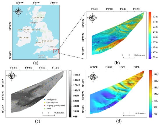
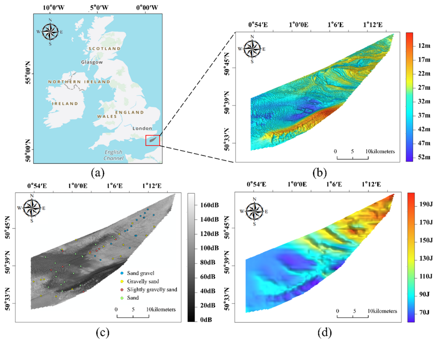
The study area is located in the southern part of the Dover Strait, a shallow-water region in the eastern English Channel, with water depths ranging from 7 m to 53 m, exhibiting a stepped steepening trend from west to east (Figure 1). Seafloor geomorphology in this region exhibits a distinct pattern: shallower bathymetry in the northeast and greater water depths toward the southwest. The water depth starts from approximately 12 m in the northeast and gradually deepens toward the southwest, exceeding 52 m at the deepest point. In the western part of the area, there is a submarine basin with a water depth of approximately 40 m, where the bottom current velocity is relatively low, and the sediments are mainly composed of Sand (S) and Slightly Gravelly Sand ((g)S). The eastern flank of the basin has a relatively steep slope; along this slope toward the east, the water depth gradually decreases, forming a submarine hill in the eastern part of the area. In this region, the bottom current velocity is relatively high, and the sediments mainly consist of Sand Gravel (sG) and Gravelly Sand (gS). The southern flank of the central basin is the steepest, and the shallowest water depth in the southernmost part of the area forms a southwest–northeast trending submarine ridge.
Figure 1.
Study area. (a) Location, (b) bathymetry, (c) backscatter intensity and samples, and (d) BCKE in the study area.
2.2. Experimental Data
The experimental data used in this study include backscatter data, bathymetric data, sediment sample data, and seafloor bottom-current kinetic energy (BCKE) data. The backscatter and bathymetric data were both acquired from survey HI1436, officially titled “Dover Strait TSS Bassurelle and Bullock Banks Bathymetric Survey (HI1436).” The backscatter data have a resolution of 5 m. A total of 60 in situ samples were collected, comprising 17 samples of gS, 18 samples of S, 17 samples of sG, and 8 samples of (g)S. The bathymetric data have a grid resolution of 2 m. They are part of the shallow-water survey outcomes from the UK Maritime and Coastguard Agency’s (MCA) Civil Hydrography Programme (CHP) 2013–2014. The backscatter data and sediment sample data were obtained from the British Geological Survey (BGS) via the GeoIndex Offshore platform [33]. The relevant bathymetric data are accessible through the Admiralty Marine Data Portal.
The BCKE dataset is formally designated as the “90th percentile kinetic energy due to currents at the seabed in the Channel and the Bay of Biscay.” The core data source is the reanalysis dataset produced by the French Research Institute for Exploitation of the Sea [34]. The integration period spans 2010 to 2015, specifically representing the average of the annual 90th percentile kinetic energy values over this period, with the vertical level precisely corresponding to the seafloor. The spatial resolution of the dataset is approximately 500 m. The kinetic energy is calculated using the classical formula:
where m is the seawater density, taken as 1027 kg/m3, and v is the current-induced velocity, with the numerical units uniformly expressed in newtons per square meter N · m−2.
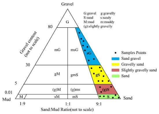
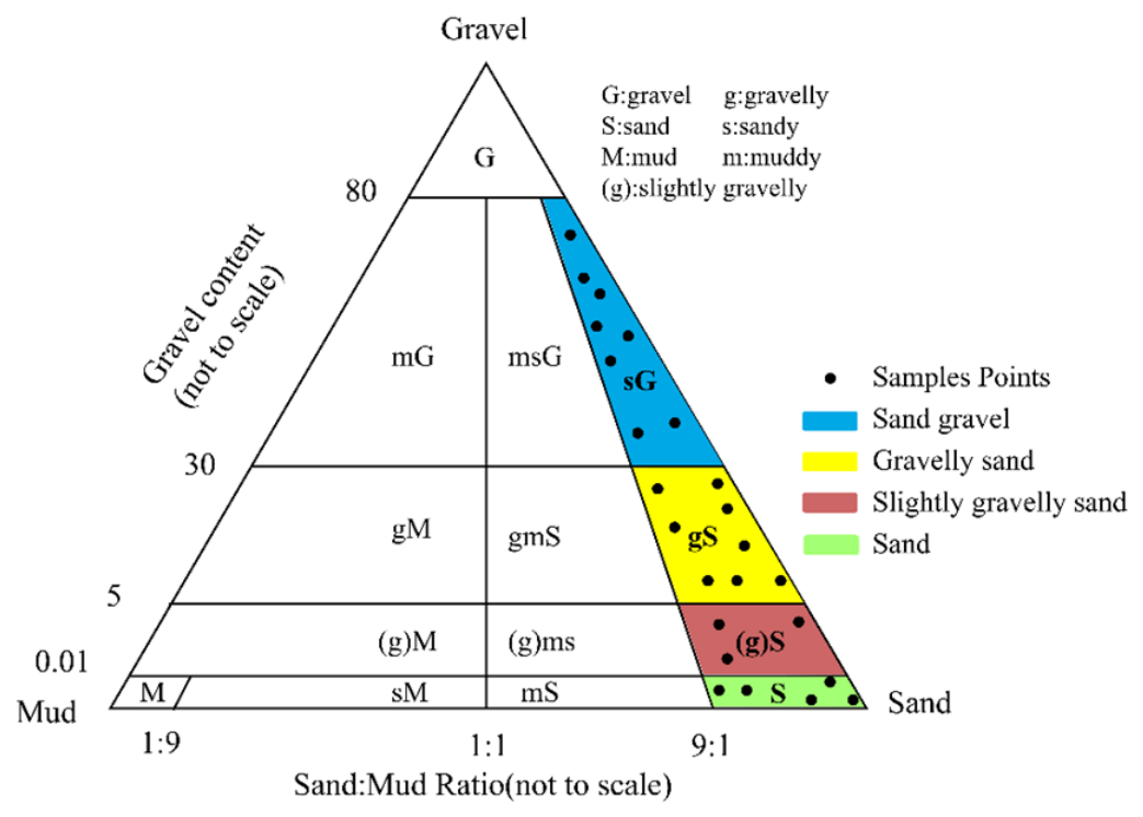
To standardize the data format and facilitate the experiments, the backscatter and bathymetric data were resampled to a resolution of 6 m. Since the BCKE data originally have a resolution of only 500 m, two interpolation methods—bilinear and cubic convolution—were applied to resample them to a 6 m resolution. For the sediment sample data, this study adopted the Folk classification standard (Figure 2). According to this standard, the sediment samples in this study are classified into four types: sG, gS, (g)S, and S.
Figure 2.
Grain-size distribution of seafloor sediment samples according to the Folk classification scheme [33].
In most seafloor classification or benthic habitat mapping studies, training sample prior information is obtained by direct manual matching with in situ ground-truth samples [35,36].
However, since acoustic surveying techniques and in situ sampling techniques generally employ different positioning systems, positional discrepancies may exist. Furthermore, during image preprocessing, the original data undergo operations such as spatial interpolation, resampling, and null-value filling, which further amplify the positional deviation of in situ sampling data relative to the backscatter data. To address this issue, this study first considered all pixels within a 5 × 5 rectangular neighborhood centered at each sampling point as sharing the same sediment type as the central sampling point, resulting in a total of 60 sampling groups. Owing to the imbalanced distribution of sampling points among the four sediment types in the study area, all sampling points of the least represented type, (g)S, were retained. Subsequently, 42 sampling groups with the highest Jeffries–Matusita (J–M) distance were selected from the remaining 52 sampling groups, yielding a final set of 50 sampling groups [37]. The J–M distance is an improved metric derived from the Bhattacharyya distance, specifically designed to quantify the “degree of separability” among multiple samples [31]. The J–M index ranges from 0 to 2.0, with higher values indicating greater separability [38], and consequently, more pronounced differences among different sediment types [39]. The resulting 1246 samples were then randomly divided into training and test sets at a ratio of 7:3 (Table 1).
Table 1.
Number of Training and Test Samples in Study Sites.
2.3. Overview and Innovation of the Framework
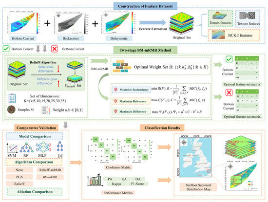
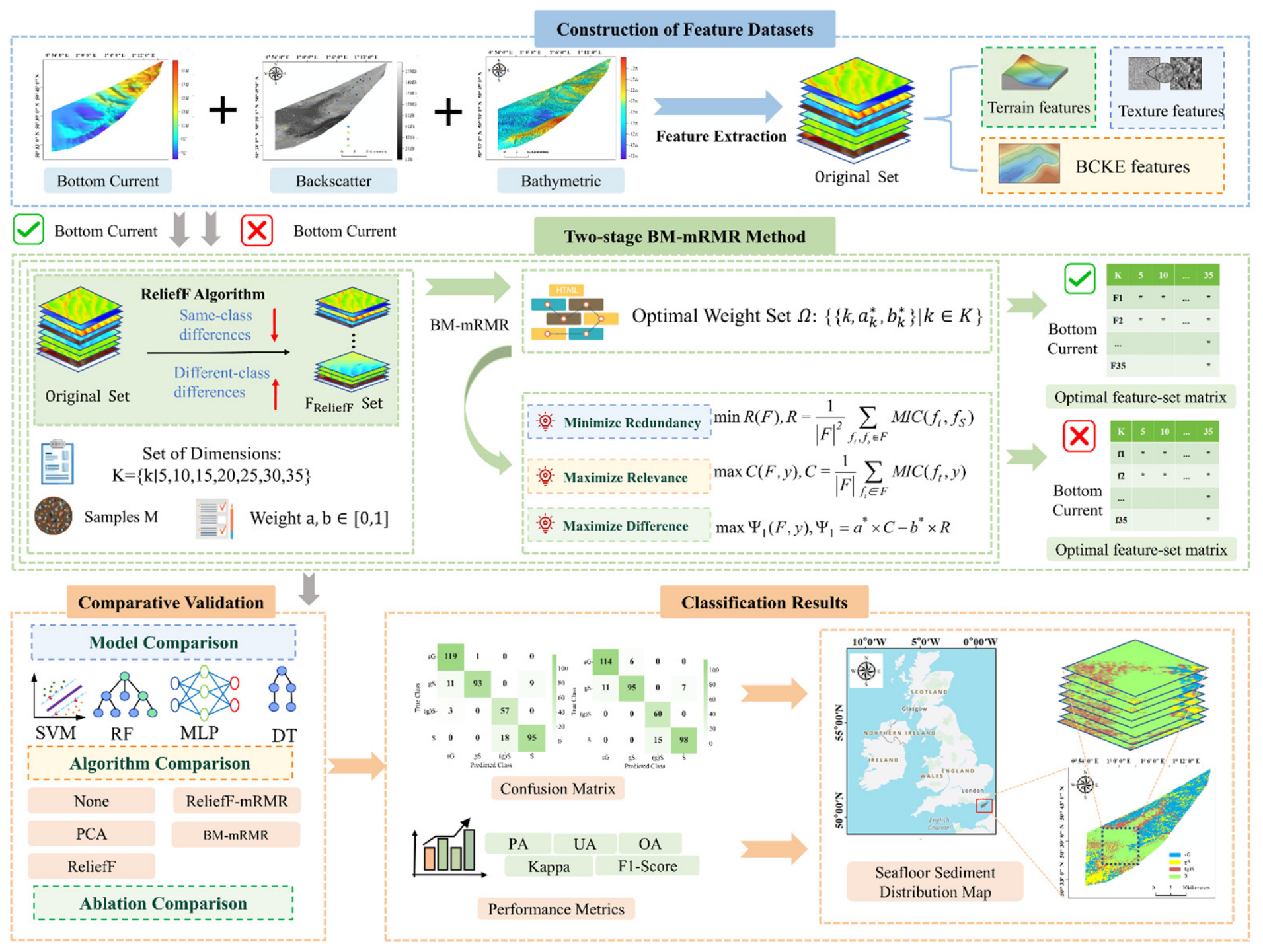
This study proposes a multi-source feature fusion method for seafloor sediment classification. The proposed method mainly includes three steps, and the overall workflow is illustrated in Figure 3. First, we extract multi-scale features from bottom current, backscatter and bathymetric data to construct two multi-source feature datasets: one integrating bathymetric and backscatter data with BCKE incorporated, and the other without BCKE. As the extracted multi-scale feature sets are high-dimensional and highly redundant, we develop a two-stage feature selection algorithm to perform feature dimensionality reduction on the two feature sets separately. Finally, neighborhood-expanded in situ samples are used as prior information, four supervised learning classifiers are adopted, and accuracy evaluation and analysis are implemented.
Figure 3.
Technical framework.
2.4. Feature Extraction
2.4.1. Backscatter and Terrain Feature Extraction
In sediment classification, multi-scale feature extraction from backscatter and bathymetric data is conducted to fully exploit the discriminative information of different sediment types in the spatial domain [40,41]. Small-scale windows (3×3 and 7×7) emphasize local textural details and scattering heterogeneity, while large-scale windows (15×15 and 25×25) characterize macroscopic features such as regional bathymetric trends and terrain continuity. Multi-scale fusion effectively compensates for the information loss caused by a single scale and enhances the discriminability among sediment classes.
2.4.2. Bottom Current Feature Extraction
In addition to the two feature types above, this study introduces BCKE features. To facilitate subsequent processing and analysis, the BCKE data were resampled to a 6 m resolution using bilinear interpolation and cubic convolution interpolation.
The bilinear interpolation formula performs linear weighting based on the four nearest neighboring points around the point to be interpolated, and is suitable for regions with smooth overall trends. The pixel value f(x,y) after interpolation is calculated as follows:
where
where (xi,yj) are the coordinates of the original pixel points, f(xi,yj) are the gray values of the original pixel points.
The cubic convolution interpolation formula utilizes 16 neighboring points and fits them via a cubic convolution kernel function, which better preserves local variation features and is suitable for regions with large gradient changes. The pixel value F(x,y) after interpolation is calculated as follows:
where (xi,yj) are the coordinates of the original pixel points, F(xi,yj) are the gray values of the original pixel points, and W(t) is the cubic convolution kernel function.
The two interpolation methods preserve large-scale trends and small-scale details, respectively. They jointly form two types of BCKE features.
2.5. Two-Stage BM-mRMR Method
In the feature extraction stage, a total of 77 multi-source features are generated by integrating acoustic, topographic and bottom current data. Due to high dimensionality, these features contain redundant and noisy information. To address this issue, this work employs the proposed two-stage BM-mRMR for feature selection. Specifically, ReliefF is first utilized for coarse screening of high-weight features, followed by BM-mRMR to refine and determine the final optimal feature subsets.
2.5.1. MIC
In 2011, the MIC was proposed by Reshef et al. as a method for measuring the correlation between two continuous variables [32,42]. This algorithm is capable of capturing various types of functional relationships and can also effectively identify non-functional associations [43], making it widely used for feature selection in machine learning.
The core concept of MIC is to discretize the relationship between two variables into a two-dimensional space and represent it using a scatter plot. The two-dimensional space is partitioned into a certain number of intervals along the x and y directions, respectively, and the MI is calculated based on the joint and marginal probability distributions. The value of MIC ranges from 0 to 1, where a higher value indicates a stronger correlation, and vice versa. The derivation process of MIC is given by the following formulas.
Given two discrete random variables X and Y, their mutual information I(X,Y) is calculated as:
where p(x,y) is the joint probability distribution of the discrete random variables; p(x) and p(y) are the marginal probability distributions of the two discrete random variables, respectively. MIC(X,Y) is calculated as:
where X and Y are two continuous variables; a and b are the number of bins for X and Y in grid partitioning; I(X,Y|a × b) is the mutual information of X and Y after being partitioned into an a × b grid. B = nk, in which k is typically assigned as 0.6 and 0.6, n refers to the total sample size [32].
2.5.2. ReliefF Algorithm
The core of ReliefF is to select features that maximize within-class similarity and between-class separability [32]. The specific procedure is as follows: in each iteration, one sediment sampling sample S is randomly selected from the training set. Then, t nearest neighbors of the same class as S (denoted as ) and t nearest neighbors from each different sediment class (denoted as ) are selected. Subsequently, the weight of each feature is updated according to the following formula:
where ω(F) is the weight of feature F. S is a randomly selected training sample, and is its j-th same-class nearest neighbor. dist (·) measures the difference between two samples with respect to feature F. t is the number of nearest neighbors, n is the number of iterations, and p(·) denotes the prior probability. is the j-th nearest neighbor from class L to sample S.
where Si[F] denotes the value of sample Si[F] with respect to feature F, and range(F) = max(F) − min(F).
In this study, the hyperparameters of ReliefF were set as t = 35 and n equal to the total number of training samples. After completing the iterative weight update, all features were sorted in descending order according to their final weights ω(F). With 77 original features, the top 40 features with the highest weights were retained in the coarse screening to construct the candidate feature set, which balances information preservation and computational efficiency and provides sufficient highly discriminative feature alternatives for the subsequent BM-mRMR fine selection.
2.5.3. BM-mRMR Algorithm
Minimum redundancy refers to minimizing the correlations among features within the selected feature subset, whereas features with high correlations are considered redundant and should be removed. Maximum relevance refers to maximizing the correlations between the selected features and the class labels. Both types of correlations are measured using MIC. The algorithmic implementation is detailed as follows.
It should be noted that the incremental scoring function of mRMR is inherently coupled with the size of the selected feature subset k. Therefore, there does not exist a single universal weight pair (a*,b*) applicable to all feature dimensions. For each predefined target feature number k, BO is employed to determine the corresponding optimal relevance–redundancy weight parameters (a*,b*) specialized for this k. The detailed BO procedure under a fixed given k is presented in Table 2.
Table 2.
Procedure of the Bo Algorithm for Determining Optimal Weight Parameters.
For a feature subset F of size k, we define the following optimization objectives:
where C denotes the average relevance between each feature in the subset F and the sample label y, and R denotes the average redundancy among features within subset F. The composite objective to be maximized is defined as:
given fixed weight parameters a* and b* (determined by BO for a specific k), a greedy incremental search strategy is employed to generate the feature subset. Assume that the existing subset Fk−1 contains (k − 1) features. The k-th feature is selected from the remaining feature set X\Fk−1 using the incremental evaluation function:
where Ψ2 denotes the incremental information gain, and X denotes the pre-filtered candidate feature set after ReliefF coarse selection.
maxΨ1(F,y),Ψ1 = a* × C − b* × R
For each candidate feature-subset size k∈{5, 10, 15, 20, 25, 30, 35}, the complete BM-mRMR pipeline is executed independently to obtain feature subsets of varying sizes. The overall accuracy corresponding to each subset is compared to determine the optimal feature dimensionality. To objectively evaluate the BM-mRMR algorithm, comparative experiments against ReliefF, ReliefF-mRMR, PCA, and the no-feature-selection baseline are carried out under the determined optimal feature dimensionality.
2.6. Classification Models and Accuracy Assessment
To validate the proposed multi-source feature fusion strategy and the BM-mRMR method, we selected four well-established supervised learning classifiers for comparative experiments. The detailed training parameters of these classifiers are provided in Table A4. These classifiers are widely used in benthic habitat mapping and remote sensing image classification.
Support Vector Machine (SVM) seeks the optimal hyperplane in a high-dimensional space via kernel function mapping [44] and exhibits strong generalization capability for small-sample, high-dimensional, and nonlinear sediment classification problems [45].
Random Forest (RF) enhances stability through bootstrap sampling and random feature selection [46]. It demonstrates outstanding generalization capability in handling high-dimensional and non-linear classification tasks.
Multilayer Perceptron (MLP) is a feedforward neural network capable of nonlinear fitting and high-level feature mining. Through its multilayer architecture, it can automatically learn complementary information among acoustic, topographic, and BCKE features, thereby improving classification accuracy for complex sediment types.
As another representative supervised machine learning model, the decision tree (DT) partitions feature space by recursively splitting feature thresholds, which can explicitly reveal the importance of multi-source seafloor sediment features.
In this study, we adopted the confusion matrix as the core evaluation tool [47]. Following the common standards in marine remote sensing and sediment mapping, we selected five metrics for comprehensive evaluation: producer’s accuracy (PA), user’s accuracy (UA), overall accuracy (OA), Kappa coefficient, and F1-score [48]. The calculation formulas for each metric are provided in Table 3.
Table 3.
Five Types of Accuracy Evaluation Metrics.
3. Results
3.1. Feature Selection Results
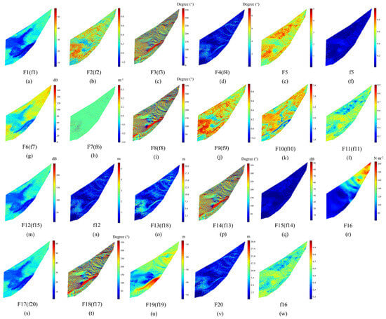
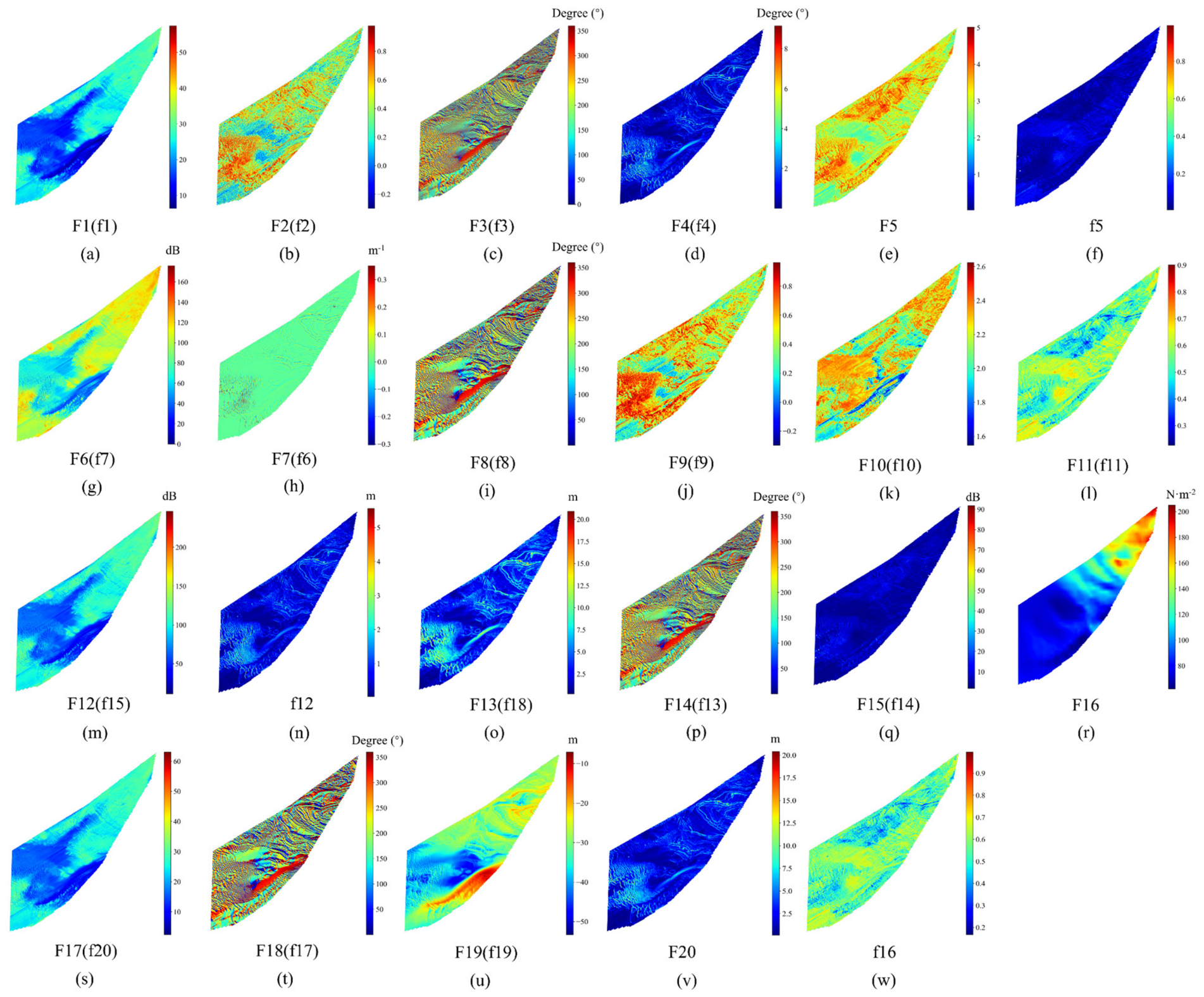
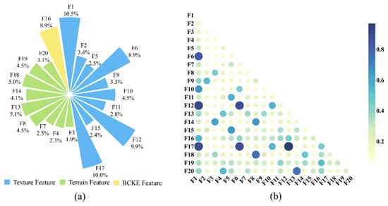
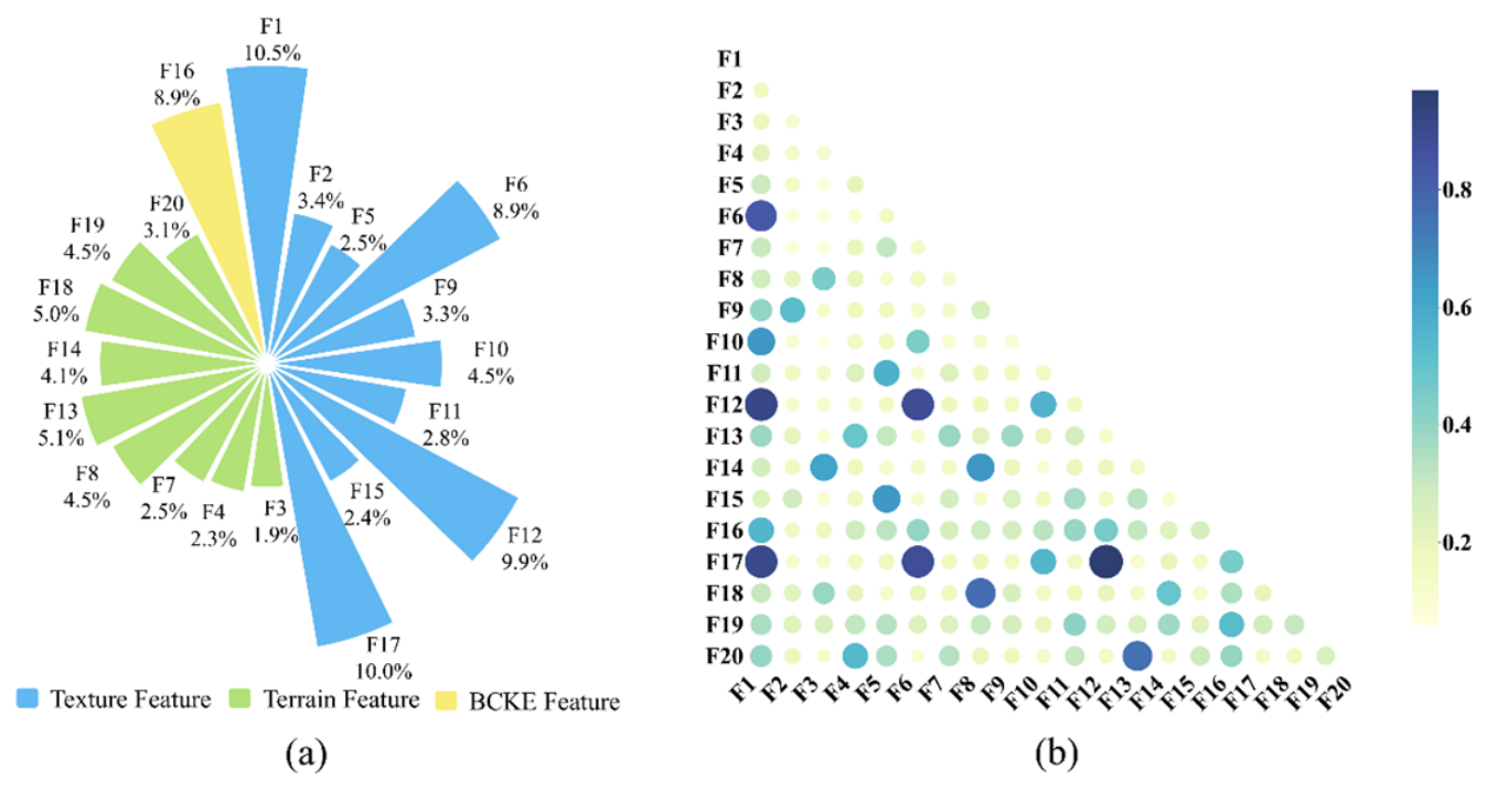
Feature selection followed the Two-Stage BM-mRMR Method proposed in this study. Specifically, ReliefF was first applied to remove features with low relevance and high redundancy from the 77 original features, followed by BM-mRMR for refined selection, ultimately determining 20 optimal features (Figure 4). The weights and correlations of the selected features are presented in Figure 5.
Figure 4.
Optimal features extracted from feature sets with and without BCKE. Here, “F” denotes the initial feature set including BCKE features, whereas “f” represents the initial feature set without BCKE features. Specific feature names are given in Table A3 in the Appendix A.
Figure 5.
Feature selection results with BCKE. (a) Weights and proportions. (b) Correlation heatmap. The colorbar denotes the maximal information coefficient (MIC) between pairwise features, ranging from 0 (statistical independence) to 1 (perfect association). All percentages are rounded to one decimal place, so their sum may not be precisely 100%. Specific feature names are given; see Table A3 in the Appendix A.
In terms of feature type composition, the selected texture features accounted for the largest proportion, reaching 58.1%, and their total proportion exceeded the sum of the other two feature types. Terrain features ranked second, accounting for 33.0%. BCKE features accounted for 8.9%, ranking fourth in contribution among the 20 selected features.
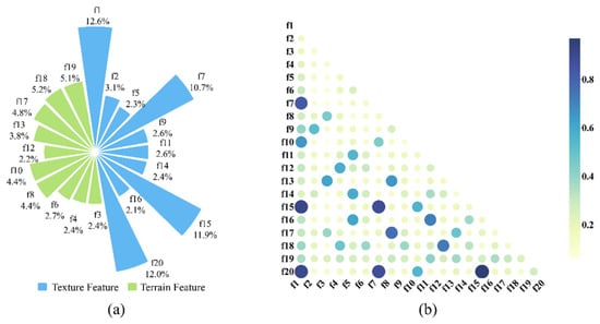
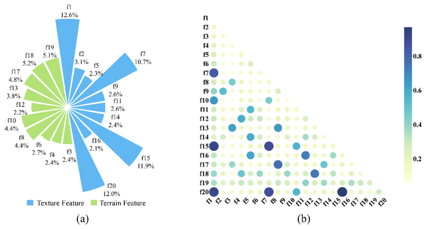
To further verify the advantages of introducing BCKE features, we established an ablation control group. Specifically, the two BCKE features were first removed from the original feature set, leaving 75 features. Under exactly the same parameters and procedures, the BM-mRMR algorithm was applied again for feature reduction and selection, yielding 20 optimal features without BCKE information (Figure 4). Their weights and feature correlations are presented in Figure 6.
Figure 6.
Feature selection results without BCKE. (a) Weights and proportions. (b) Correlation heatmap. The colorbar denotes the maximal information coefficient (MIC) between pairwise features, ranging from 0 (statistical independence) to 1 (perfect association). All percentages are rounded to one decimal place, so their sum may not be precisely 100%. Specific feature names are given; see Table A3 in the Appendix A.
After the removal of BCKE features, 10 texture features were selected, accounting for 62.5% of the total weight, while 10 terrain features were selected, accounting for 37.5%. This indicates that terrain information, as a traditional classification means, can effectively complement texture features and enhance the completeness of sediment classification.
3.2. Results of Ablation Experiments
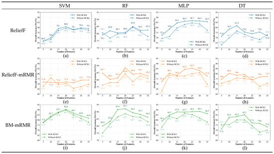
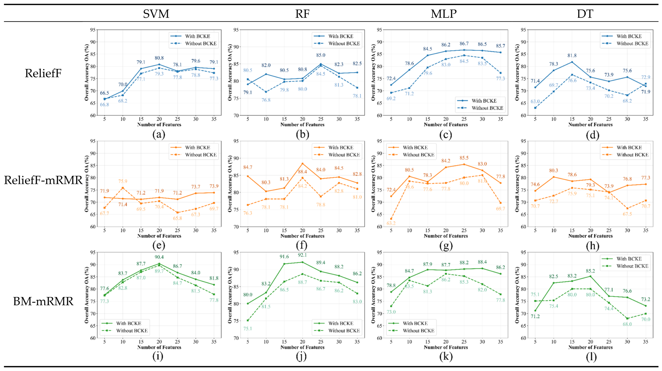
To quantify the contribution of BCKE features to classification accuracy, we compared overall accuracy (OA) with and without BCKE under four classifiers, three feature selection schemes and seven feature dimensions (Figure 7).
Figure 7.
Results of 4 classifiers and 3 algorithms with/without BCKE features. (a) ReliefF+SVM; (b) ReliefF+RF; (c) ReliefF+MLP; (d) ReliefF+DT; (e) ReliefF-mRMR+SVM; (f) ReliefF-mRMR+RF; (g) ReliefF-mRMR+MLP; (h) ReliefF-mRMR+DT; (i) BM-mRMR+SVM; (j) BM-mRMR+RF; (k) BM-mRMR+MLP; (l) BM-mRMR+DT.
The maximum average OA gain of 4.91% brought by BCKE appears for the DT classifier combined with ReliefF. The largest individual OA increments reach 8.6% (DT, 10 features, ReliefF; OA: 78.3% vs. 69.7%), 9.2% (MLP, 5 features; OA: 72.4% vs. 63.2%), 8.4% (RF, 5 features, ReliefF-mRMR; OA: 84.7% vs. 76.3%), and 6.4% (SVM, 30 features, ReliefF-mRMR; OA: 73.7% vs. 67.3%).
OA increases in 92.86% of all 84 test groups (78 cases). Only 6 groups show accuracy degradation, with a maximum drop of merely 4.5% (SVM, 10 features, ReliefF-mRMR). BCKE features yield positive contributions across most experimental setups.
3.3. Experimental Results of Different Algorithms
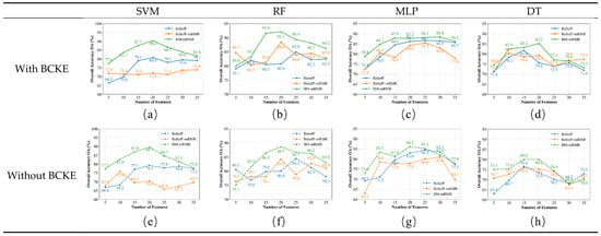
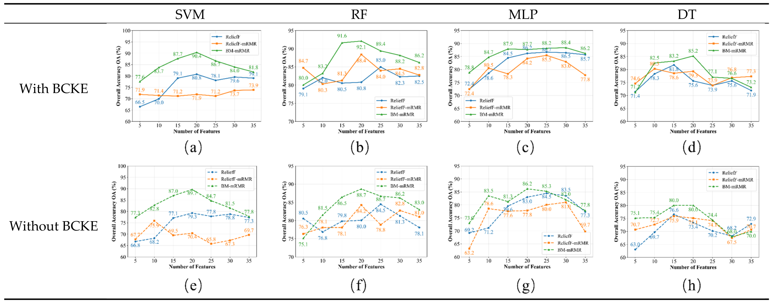
To verify the superiority of BM-mRMR, we compared it with ReliefF and ReliefF-mRMR. We evaluated the classification accuracy of the feature subsets obtained by each algorithm using four classifiers—SVM, RF, MLP and DT (Figure 8).
Figure 8.
Comparison results of 4 classifiers and 3 algorithms with and without BCKE features. (a) SVM with BCKE; (b) RF with BCKE; (c) MLP with BCKE; (d) DT with BCKE; (e) SVM without BCKE; (f) RF without BCKE; (g) MLP without BCKE; (h) DT without BCKE.
In terms of optimal OA (Table 4), BM-mRMR achieves the highest accuracy with and without BCKE. With BCKE, the optimal OA values of SVM, RF, MLP and DT are 90.4%, 92.1%, 88.4% and 85.2%, respectively; without BCKE, the corresponding values are 89.7%, 88.7%, 86.2% and 80.0%. The highest accuracies of ReliefF and ReliefF-mRMR reach 86.7% and 88.4%, both below 89%. Overall, BM-mRMR outperforms other schemes across most configurations.
Table 4.
Optimal accuracy of different combinations.
For the BM-mRMR algorithm, the optimal feature dimensionality was 20 in 7 of the 8 experimental groups, and 30 features in the remaining group. In that group, using 20 features yielded an accuracy of 87.7%, only 0.7% lower than the optimal 88.4% achieved with 30 features. To further verify the advantages of the BM-mRMR algorithm, this study selects 20 as the optimal feature dimensionality. It then compared classification performance across sediment types among five schemes: BM-mRMR, PCA, ReliefF, ReliefF-mRMR, and no feature reduction (Table 5).
Table 5.
Model Evaluation Results With Different Inputs.
As shown in Table 5, under the optimal 20-feature configuration, the BM-mRMR algorithm significantly outperformed the comparison schemes. Taking the RF classifier as an example, the algorithm achieved UA values of 98.86%, 98.21%, 90.84%, and 77.33% for gS, S, sG, and (g)S, respectively, and PA values of 76.99%, 97.35%, 99.17%, and 96.67%, respectively. In contrast, without feature selection, the UA and PA for gS were both only 77.88%, indicating that the original high-dimensional features contained substantial redundancy and noise, which interfered with the model’s accurate identification of the gravelly sand class. Although PCA reduced the feature space, the PA for gS dropped to 53.98%, suggesting that linear transformation struggled to preserve the nonlinear discriminative information required for sediment classification.
3.4. Classification Results
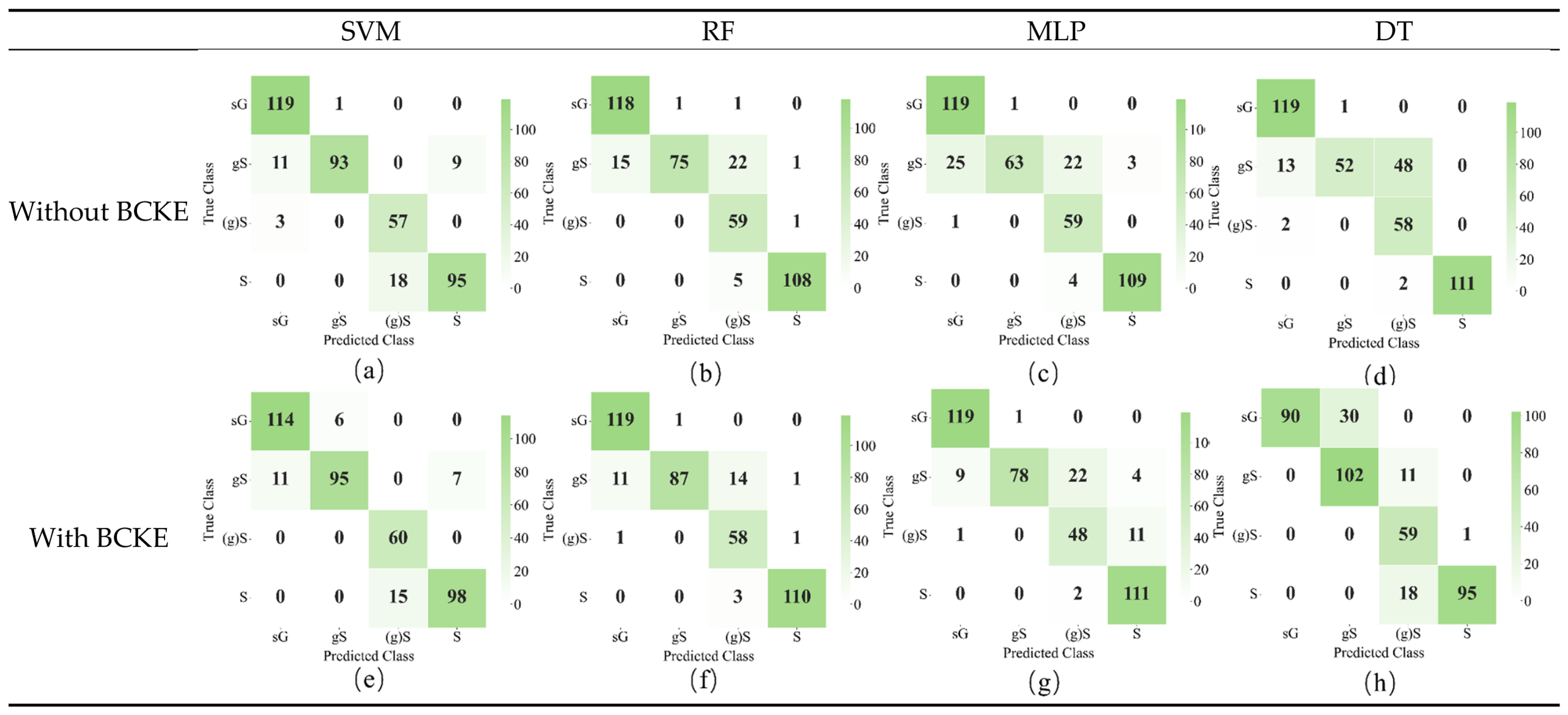
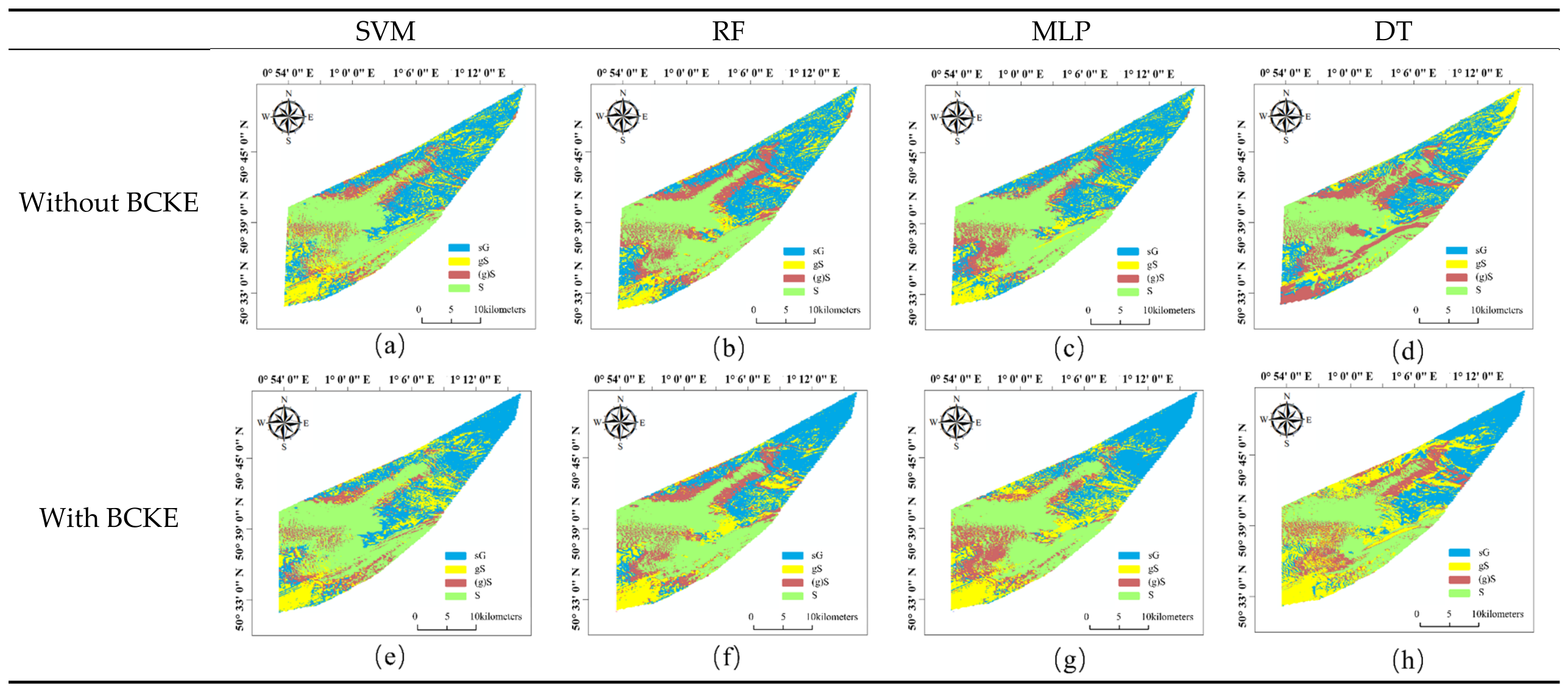
To visually demonstrate the classification performance of the proposed BM-mRMR algorithm under the optimal feature configuration, confusion matrices (Figure 9) and sediment distribution maps (Figure 10) were generated for both scenarios with and without BCKE.
Figure 9.
Confusion matrix results of sediment classification. (a) SVM without BCKE; (b) RF without BCKE; (c) MLP without BCKE; (d) DT without BCKE; (e) SVM with BCKE; (f) RF with BCKE; (g) MLP with BCKE; (h) DT with BCKE.
Figure 10.
Sediment distribution map. (a) SVM without BCKE; (b) RF without BCKE; (c) MLP without BCKE; (d) DT without BCKE; (e) SVM with BCKE; (f) RF with BCKE; (g) MLP with BCKE; (h) DT with BCKE.
After the introduction of BCKE features, the total number of misclassified samples decreased for all four classifiers. The most notable improvement was observed for RF (from 46 to 32), followed by MLP (from 56 to 50), DT (from 66 to 60), and SVM (from 42 to 39). This result further confirms the positive contribution of BCKE features to sediment classification accuracy, consistent with the quantitative analysis presented earlier, although the magnitude of improvement varied slightly among classifiers.
4. Discussion
4.1. Interpretation of Feature Selection
When the data source included BCKE features, the BCKE features accounted for 8.9% of the total weight in the selected feature set, ranking fourth in contribution. In terms of correlation, the coefficients between BCKE features and texture or terrain features were generally below 0.4, indicating that BCKE carries information independent of acoustic and topographic features. When BCKE features were excluded, 10 texture features and 10 terrain features were selected, with weights of 62.5% and 37.5%, respectively. The internal correlations within the terrain feature set varied significantly with scale differentiation, suggesting that multi-scale terrain parameters can be effectively decoupled. The average correlation coefficients between texture and terrain features were generally low, indicating that the two feature types capture different attribute dimensions of the sediment [49].
4.2. Hydrodynamic Contributions to Classification
Across all 84 experimental combinations, the introduction of BCKE features improved the OA by 3.48% on average, with a maximum improvement of 9.4%. Among the four classifiers, MLP benefited most significantly, with an average improvement of 4.71%, followed by DT with 4.50%, RF with 2.90%, and SVM with 1.80%.
The physical basis of this improvement lies in the fundamental principles of sediment transport. According to the Shields criterion and the subsequently developed bed-load transport theories [50,51], the boundary shear stress exerted by bottom currents on the seabed determines the threshold for sediment particle entrainment. The 90th percentile kinetic energy adopted in this study effectively characterizes the high-tail flow conditions that govern intermittent sediment mobilization [52,53]. In the Dover Strait study area, BCKE values on the eastern steep slope generally exceeded 110 N·m−2, corresponding to coarse-grained sediments such as gS and sG, while the central basin exhibited BCKE values below 90 N·m−2, dominated by continuous S distribution. This spatial correspondence—coarse sediments in high-energy areas and fine sediments in low-energy areas—is fully consistent with the classic Hjulström–Sundborg diagram [54].
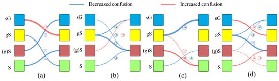
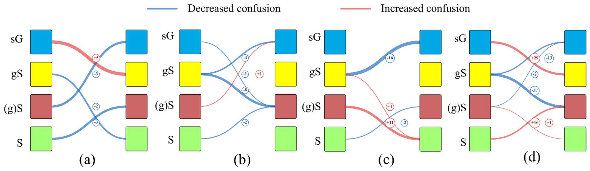
To validate the incremental value of BCKE features, we compared the classification confusion of several pairs of easily confusable sediment types before and after introducing BCKE across four classifiers. Figure 9 presents the confusion matrices under the optimal feature configuration, while Figure 11 uses Sankey diagrams to directly visualize the changes in misclassification flows after BCKE introduction, where blue links indicate a decrease in misclassification count and red links indicate an increase.
Figure 11.
Sankey diagrams showing the changes in misclassification flows after BCKE introduction for (a) SVM, (b) RF, (c) MLP and (d) DT. Left nodes represent true sediment classes, and right nodes represent predicted classes. Link thickness is proportional to the magnitude of change, and numbers indicate the change in misclassified sample count relative to the no-BCKE scenario. Blue links indicate a decrease in misclassification count (improvement), and red links indicate an increase (deterioration).
Specifically, the four classifiers responded differently to BCKE features. RF achieved stable improvements: misclassifications of gS → (g)S and gS → sG dropped by 8 and 4, with reductions across most major confusion pairs. MLP obtained the largest single-class gain, reducing gS → sG errors by 16, while sG → (g)S misclassifications rose by 11. SVM was barely affected, with only five extra sG → gS errors and limited overall performance change.
For DT, BCKE greatly reduced confusion between gS and (g)S, cutting gS → sG and gS → (g)S misclassifications by 13 and 37. However, new confusions appeared: sG → gS and S → (g)S errors increased by 29 and 16. BCKE improved the separability of gS but weakened discrimination for sG and S and aggravated their mutual confusion.
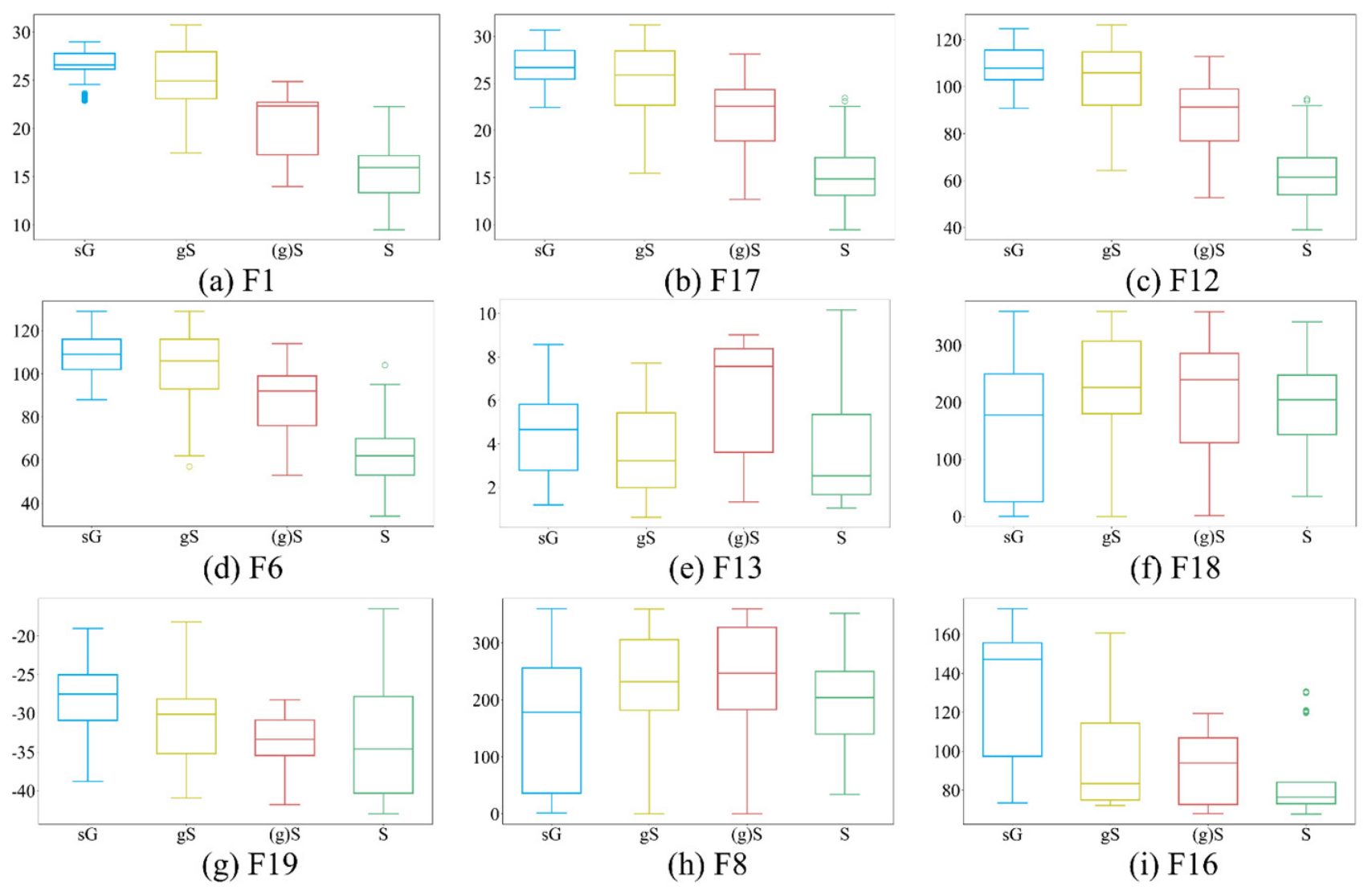
The introduction of BCKE features enables the classification model to perceive the energy conditions of the sedimentary environment. To this end, boxplots were generated to illustrate the numerical distributions of the top nine selected features under the scenario with BCKE (Figure 12). The top four features in terms of importance (F1, F17, F12, F6) all belonged to texture features, indicating their high contribution to sediment discrimination; however, features of other types are still needed to further improve classification accuracy and interpretability. In Figure 12(i), samples of sG (coarser mean grain size) generally exhibited higher BCKE values, while samples of S (finer mean grain size) showed relatively lower BCKE values, with significant overall differences across sediment types.
Figure 12.
Boxplots of the top 9 highest-weight features after feature selection with BCKE features incorporated. F1, F17, F12, and F6 are texture features. F13, F18, F19, and F8 are terrain features. F16 is BCKE feature. Dots denote outliers. Specific feature names are given; see Table A3 in the Appendix A.
In high-BCKE environments, bottom currents scour fine particles, increasing the relative proportion of gravel and shifting the sediment toward gravelly sand; conversely, low-BCKE environments favor the preservation of fine particles, diluting the gravel component and shifting the sediment toward slightly gravelly sand [55].
4.3. Advantages of BM-mRMR Algorithm
As shown in Table 6, BM-mRMR achieved both the optimal OA and the best average OA across all eight comparison groups, and its advantage was not dependent on a specific classifier or the presence of BCKE features.
Table 6.
Average accuracy of different combinations.
Notably, ReliefF and ReliefF-mRMR delivered similar accuracies for RF under BCKE augmentation (81.74% versus 83.71%). For SVM, however, ReliefF-mRMR dropped to 72.17%, underperforming ReliefF (76.17%); this gap further expanded without BCKE (69.47% vs. 75.04%). The 5.57-percentage-point degradation indicates that the second-stage mRMR filtering may discard nonlinearly informative features. Since SVM relies heavily on high-order feature interactions, removing such critical features yields obvious performance loss. For DT, by comparison, ReliefF-mRMR consistently outperformed ReliefF for both settings: 77.27% vs. 75.51% with BCKE and 72.38% vs. 70.58% without BCKE. DT’s inherent internal feature-pruning mechanism enables it to accommodate the truncated feature subsets, so it suffers little negative impact from mRMR feature elimination. These contrasting outcomes show that the applicability of ReliefF-mRMR depends on classifier properties and is not governed purely by input-feature quality.
In contrast, BM-mRMR consistently achieved optimal results across all classifiers. Its advantage was most noticeable on SVM—8.39% and 12.39% above ReliefF and ReliefF-mRMR, respectively, with BCKE, and 7.93% and 13.50% above them without BCKE. These results suggest that the proposed method offers good adaptability across different classifiers.
The proposed BM-mRMR feature selection algorithm tends to outperform ReliefF and ReliefF-mRMR in terms of both average and optimal accuracies. Its potential advantages can be attributed to two aspects. First, it uses MIC to capture nonlinear associations—both between features and labels, and among features themselves—which helps compensate for the limited sensitivity of MI to nonlinear relationships [32]. Second, it employs BO to adaptively balance relevance and redundancy weights, thereby mitigating the potential bias associated with fixed weights in conventional mRMR. These mechanisms may collectively contribute to the effectiveness of BM-mRMR in selecting features from high-dimensional, nonlinear, and multi-source seafloor sediment data.
4.4. Interpretation of Sediment Distribution
The northeastern part of the study area is characterized by shallow water depths, minor topographic relief, relatively strong backscatter intensity, and a northeastward increasing trend in BCKE, indicating a high-energy hydrodynamic environment. The southwestern gentle slope zone has moderate water depth (approximately 30 m), moderate backscatter intensity, and moderate BCKE. The central basin exhibits flat bathymetry, weak backscatter, and low BCKE, representing a typical low-energy fine-grained depositional area (Figure 1).
As shown in Figure 10, the northeastern and southwestern gentle slope zones exhibited the most typical contrast before and after the introduction of BCKE features. In the northeastern gentle slope zone, without BCKE, the sG distribution was scattered and notably smaller, with many sG samples misclassified as gS in disordered patchy patterns. After introducing BCKE, the sG distribution expanded significantly into continuous bands, with misclassifications substantially eliminated. In the southwestern gentle slope zone, without BCKE, the gS distribution was excessively large and chaotically extended, with substantial misclassification of gS as sG. After introducing BCKE, the misclassified sG samples within the gS distribution decreased significantly.
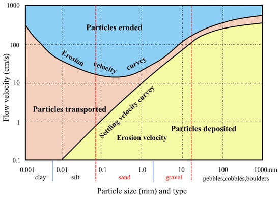
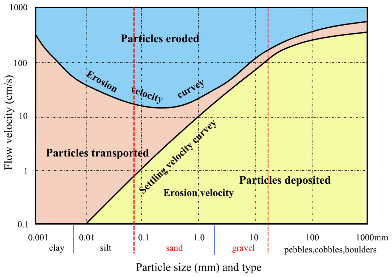
The above spatial patterns can be qualitatively interpreted through the Hjulström–Sundborg diagram [55]. The spatial distribution of seafloor sediment grain size is fundamentally controlled by near-bottom hydrodynamic conditions [54,56]. The Hjulström–Sundborg diagram (Figure 13) qualitatively characterizes the response of particles with different grain sizes to flow velocity variations, delineating erosion, transportation, and deposition regimes [57]. It should be noted that this diagram is derived from empirical observations in fluvial environments [55]; in this study, it is employed for qualitative analysis of seafloor sedimentary processes, with BCKE serving as a proxy for seabed current velocity rather than directly applying the quantitative velocity values in the diagram.
Figure 13.
Hjulström–Sundborg diagram showing the relationships among flow velocity, sediment particle size, and erosion–transport–deposition processes.Vertical blue lines mark the boundaries of different sediment particle size classes. The particle-size range between red dashed lines corresponds to sediment grain sizes within the study area [55].
According to the diagram, the critical velocity required for the initiation (erosion) of coarse sand and gravel-sized particles is substantially higher than that for fine sand and silt fractions; however, once mobilized, the critical velocity for their deposition is conversely lower than that for fine-grained materials [56,57]. This implies that the resuspension and transport of coarse-grained sediments require relatively strong hydrodynamic conditions, whereas fine-grained sediments can be eroded under weaker dynamic conditions and settle only under even weaker flow regimes.
Correlating this physical framework with the spatial distribution of BCKE in the study area provides a clear explanation for the sediment type differentiation across different geomorphic units. In the northeastern gentle slope zone, BCKE values generally exceed 110 N·m−2, indicating a persistently high-energy environment capable of eroding and transporting fine to medium sand particles, maintaining fine-grained fractions in prolonged resuspension and preventing their in situ deposition. This process leads to the relative enrichment of gravel components, forming coarse-grained deposits dominated by sG. Conversely, in the central basin, BCKE values remain below 90 N·m−2, indicating a low-energy regime that only sustains the transport of silt and clay fractions, while sand-sized and coarser particles undergo rapid settling. This environment favors the continuous accumulation and preservation of fine-grained materials, resulting in a sedimentary pattern dominated by S. The southwestern gentle slope zone represents a transitional hydrodynamic environment, with BCKE values falling between those of the two aforementioned zones. Here, bottom currents are capable of intermittently transporting fine gravel and coarse sand fractions but are insufficient to sustain the concentrated accumulation of coarse-grained components over extended periods, thereby giving rise to a transitional coexistence of gS and sG.
It is noteworthy that although both the northeastern and southwestern gentle slope zones belong to gentle slope geomorphic units, their sedimentary responses are fundamentally different—a distinction that topographic and backscatter features alone cannot capture. The introduction of BCKE features precisely fills this physical information gap. The qualitative interpretation through the Hjulström–Sundborg diagram provides sedimentary dynamics-based mechanistic support for the spatial differentiation of sediment types observed in the classification results [54].
It should be further noted that the Hjulström–Sundborg diagram describes the simplified behavior of individual particles under uniform flow conditions [56]. In actual seafloor environments, the critical entrainment velocity of particles is also influenced by sediment cohesion, bedform morphology, bioturbation, and near-bottom turbulence structure [58,59,60,61]. Therefore, the above analysis constitutes a qualitative-level dynamic interpretation, intended to provide physical logical support for the spatial correspondence between BCKE features and sediment types, rather than serving as a basis for quantitative velocity conversion. This demonstrates that BCKE, as a representative indicator of hydrodynamic factors, can not only improve classification accuracy from a statistical perspective but also enhance the sedimentary genetic interpretability of classification results from a physical standpoint.
5. Conclusions
This paper proposes BCTBM, a bottom-current-fused two-stage BM-mRMR method for seafloor sediment classification, to address the limited physical interpretability and unsatisfactory classification accuracy of conventional seafloor sediment classification. This approach incorporates BCKE into multi-source features and establishes a two-stage feature-selection architecture. It first performs coarse screening on the original feature set via ReliefF, then adopts the BM-mRMR module for fine feature selection. The maximal information coefficient (MIC) is utilized to explore nonlinear correlations among features, and Bayesian optimization (BO) adaptively balances feature relevance and redundancy, enabling BCTBM to compute optimal relevance–redundancy weights for diverse datasets.
Experiments based on the eastern English Channel dataset verify the competitive advantages of BCTBM. BCKE provides complementary hydrodynamic information and mitigates classification confusion for sediments with similar acoustic and topographic signatures. The classification results are consistent with the classic Hjulström–Sundborg sedimentary dynamic theory. Nevertheless, one practical limitation should be pointed out: the original BCKE dataset has a coarse native resolution of 500 m. Interpolation is implemented to match the 6 m resolution of acoustic–topographic features, which may produce artefacts and impair classification accuracy in near-shore areas with steep hydrodynamic gradients. And BCKE governs sediment distribution, dominant sediment-controlling factors differ among marine environments, e.g., abyssal plains, coral reef platforms and muddy tidal flats. Further exploration of multi-dimensional physical factors is required to build a sediment-classification framework adaptable to diverse marine environments.
Author Contributions
Conceptualization, B.Z., Z.Q. and B.M.; methodology, B.Z.; software, B.M.; validation, B.Z.; formal analysis, B.Z.; investigation, B.Z.; resources, Z.Q.; data curation, B.M.; writing—original draft preparation, B.Z. and B.L.; writing—review and editing, B.Z. and X.C.; visualization, B.Z.; supervision, Z.Q.; project administration, Z.Q. and J.W.; funding acquisition, B.M. All authors have read and agreed to the published version of the manuscript.
Funding
This research was funded by the Taishan Scholars Program, Shandong Provincial Natural Science Foundation (grant number ZR2024QD082), National Natural Science Foundation of China (grant number 42676083).
Data Availability Statement
Backscatter data and sample point data used in this experiment are available from https://mapapps2.bgs.ac.uk/geoindex_offshore/home.html (accessed on 1 April 2026). Bathymetric data can be obtained from https://data.admiralty.co.uk/portal/apps/sites/#/marine-data-portal (accessed on 1 April 2026). Bottom-current kinetic energy (BCKE) data are accessible at -855d-43de-8370-40ff8e4d9542/.
Acknowledgments
The authors want to thank the British Geological Survey (BGS) for providing the multibeam backscatter data and in situ sediment ground-truth samples via the GeoIndex Offshore platform, the UK Hydrographic Office for providing bathymetric datasets from the Admiralty Marine Data Portal, and the French Research Institute for Exploitation of the Sea (IFREMER) for providing the reanalysis dataset of bottom-current kinetic energy for the English Channel and Bay of Biscay, and thank the Taishan Scholars Program and Shandong Provincial Natural Science Foundation (grant number ZR2024QD082) for the financial support of this research, and thank the editors and reviewers for their valuable comments and suggestions to improve the manuscript.
Conflicts of Interest
The authors declare no conflicts of interest.
Abbreviations
| BM-mRMR | Bayesian MIC-augmented Minimum Redundancy Maximum Relevance |
| BCKE | Bottom-Current Kinetic Energy |
| J-M | Jeffries–Matusita |
| BO | Bayesian Optimization |
| mRMR | Minimum Redundancy Maximum Relevance |
| PCA | Principal Component Analysis |
| RF | Random Forest |
| MI | Mutual Information |
| DT | Decision Tree |
| SVM | Support Vector Machine |
| MLP | Multilayer Perceptron |
| sG | Sand Gravel |
| gS | Gravelly Sand |
| (g)S | Slightly Gravelly Sand |
| S | Sand |
Appendix A
Appendix A.1
Table A1.
Calculation Formulas of Terrain Features.
Appendix A.2
Table A2.
Calculation Formulas of Backscatter Features.
Appendix A.3
Table A3.
Nomenclature of feature names.
Appendix A.4
Table A4.
Model Parameters.
References
- Kostylev, V.E.; Todd, B.J.; Fader, G.B.J.; Courtney, R.C.; Cameron, G.D.M.; Pickrill, R.A. Benthic Habitat Mapping on the Scotian Shelf Based on Multibeam Bathymetry, Surficial Geology and Sea Floor Photographs. Mar. Ecol. Prog. Ser. 2001, 219, 121–137. [Google Scholar] [CrossRef] [Scilit]
- Brown, C.J.; Smith, S.J.; Lawton, P.; Anderson, J.T. Benthic Habitat Mapping: A Review of Progress Towards Improved Understanding of the Spatial Ecology of the Seafloor Using Acoustic Techniques. Estuar. Coast. Shelf Sci. 2011, 92, 502–520. [Google Scholar] [CrossRef] [Scilit]
- Valkovic, V.; Matika, D.; Kollar, R.; Obhodas, J.; Sudac, D. Environmental Security of the Adriatic Coastal Sea Floor. IEEE Trans. Nucl. Sci. 2010, 57, 2724–2731. [Google Scholar] [CrossRef] [Scilit]
- Wang, H.; Zhou, Q.; Wei, S.; Xue, X.; Zhou, X.; Zhang, X. Research on Seabed Sediment Classification Based on the MSC-Transformer and Sub-Bottom Profiler. J. Mar. Sci. Eng. 2023, 11, 1074. [Google Scholar] [CrossRef] [Scilit]
- Mestdagh, S.; Amiri-Simkooei, A.; van der Reijden, K.J.; Koop, L.; O’FLynn, S.; Snellen, M.; Van Sluis, C.; Govers, L.L.; Simons, D.G.; Herman, P.M.; et al. Linking the Morphology and Ecology of Subtidal Soft-Bottom Marine Benthic Habitats: A Novel Multiscale Approach. Estuar. Coast. Shelf Sci. 2020, 238, 106687. [Google Scholar] [CrossRef] [Scilit]
- Lamarche, G.; Lurton, X. Recommendations for Improved and Coherent Acquisition and Processing of Backscatter Data from Seafloor-Mapping Sonars. Mar. Geophys. Res. 2018, 39, 5–22. [Google Scholar] [CrossRef] [Scilit]
- Li, D.; Tang, C.; Xia, C.; Zhang, H. Acoustic Mapping and Classification of Benthic Habitat Using Unsupervised Learning in Artificial Reef Water. Estuar. Coast. Shelf Sci. 2017, 185, 11–21. [Google Scholar] [CrossRef] [Scilit]
- Hutin, E.; Simard, Y.; Archambault, P. Acoustic Detection of a Scallop Bed from a Single-Beam Echosounder in the St. Lawrence. ICES J. Mar. Sci. 2005, 62, 966–983. [Google Scholar] [CrossRef] [Scilit]
- Lee, C.; Park, S.; Yoon, D.; Yi, B.Y.; Lim, M. Enhancing Seabed Sediment Classification with Multibeam Echo-Sounding and Self-Training: A Case Study from the East Sea of South Korea. Front. Earth Sci. 2025, 13, 1550244. [Google Scholar] [CrossRef] [Scilit]
- Khomsin; Mukhtasor; Pratomo, D.G.; Suntoyo. The Development of Seabed Sediment Mapping Methods: The Opportunity Application in the Coastal Waters. IOP Conf. Ser. Earth Environ. Sci. 2021, 731, 012039. [Google Scholar] [CrossRef] [Scilit]
- Kruss, A.; Madricardo, F.; Sigovini, M.; Ferrarin, C.; Montereale-Gavazzi, G. Assessment of Submerged Aquatic Vegetation Abundance Using Multibeam Sonar in Very Shallow and Dynamic Environment: The Lagoon of Venice (Italy) Case Study. In Proceedings of the RIO Acoustics 2015, IEEE/OES Acoustics in Underwater Geosciences Symposium; CPRM: Rio de Janeiro, Brazil, 2015; p. 16. [Google Scholar]
- De, C.; Chakraborty, B. Model-Based Acoustic Remote Sensing of Seafloor Characteristics. IEEE Trans. Geosci. Remote Sens. 2011, 49, 3868–3877. [Google Scholar] [CrossRef]
- Valentine, P.C.; Todd, B.J.; Kostylev, V.E. Classification of Marine Sublittoral Habitats, with Application to the Northeastern North America Region. In Proceedings of the American Fisheries Society Symposium; American Fisheries Society: Bethesda, MD, USA, 2005; Volume 41, pp. 183–200. [Google Scholar]
- Shumchenia, E.J.; King, J.W. Comparison of Methods for Integrating Biological and Physical Data for Marine Habitat Mapping and Classification. Cont. Shelf Res. 2010, 30, 1717–1729. [Google Scholar] [CrossRef] [Scilit]
- Pillay, T.; Cawthra, H.C.; Lombard, A.T. Characterisation of Seafloor Substrate Using Advanced Processing of Multibeam Bathymetry, Backscatter, and Sidescan Sonar in Table Bay, South Africa. Mar. Geol. 2020, 429, 106332. [Google Scholar] [CrossRef] [Scilit]
- Lark, R.M.; Marchant, B.P.; Dove, D.; Green, S.L.; Stewart, H.; Diesing, M. Combining Observations with Acoustic Swath Bathymetry and Backscatter to Map Seabed Sediment Texture Classes: The Empirical Best Linear Unbiased Predictor. Sediment. Geol. 2015, 328, 17–32. [Google Scholar] [CrossRef] [Scilit]
- Ierodiaconou, D.; Schimel, A.C.G.; Kennedy, D.; Monk, J.; Gaylard, G.; Young, M.; Diesing, M.; Rattray, A. Combining Pixel and Object Based Image Analysis of Ultra-High Resolution Multibeam Bathymetry and Backscatter for Habitat Mapping in Shallow Marine Waters. Mar. Geophys. Res. 2018, 39, 271–288. [Google Scholar] [CrossRef] [Scilit]
- Menandro, P.S.; Misiuk, B.; Brown, C.J.; Bastos, A.C. Multispectral Multibeam Backscatter Response of Heterogeneous Rhodolith Beds. Sci. Rep. 2023, 13, 20220. [Google Scholar] [CrossRef] [Scilit]
- Diesing, M.; Mitchell, P.; Stephens, D. Image-Based Seabed Classification: What Can We Learn from Terrestrial Remote Sensing? ICES J. Mar. Sci. 2016, 73, 2425–2441. [Google Scholar] [CrossRef] [Scilit]
- Hughes, G. On the Mean Accuracy of Statistical Pattern Recognizers. IEEE Trans. Inf. Theory 1968, 14, 55–63. [Google Scholar] [CrossRef] [Scilit]
- Anokye, M.; Cui, X.; Yang, F.; Wang, P.; Sun, Y.; Ma, H.; Amoako, E.O. Optimizing Multi-Classifier Fusion for Seabed Sediment Classification Using Machine Learning. Int. J. Digit. Earth 2024, 17, 2295988. [Google Scholar] [CrossRef] [Scilit]
- Eleftherakis, D.; Amiri-Simkooei, A.; Snellen, M.; Simons, D.G. Improving Riverbed Sediment Classification Using Backscatter and Depth Residual Features of Multi-Beam Echo-Sounder Systems. J. Acoust. Soc. Am. 2012, 131, 3710–3725. [Google Scholar] [CrossRef] [Scilit]
- Cui, X.; Yang, F.; Wang, X.; Ai, B.; Luo, Y.; Ma, D. Deep Learning Model for Seabed Sediment Classification Based on Fuzzy Ranking Feature Optimization. Mar. Geol. 2021, 432, 106390. [Google Scholar] [CrossRef] [Scilit]
- Wang, Y.; Qi, Q.; Liu, Y. Unsupervised Segmentation Evaluation Using Area-Weighted Variance and Jeffries-Matusita Distance for Remote Sensing Images. Remote Sens. 2018, 10, 1193. [Google Scholar] [CrossRef] [Scilit]
- Padma, S.; Sanjeevi, S. Jeffries Matusita Based Mixed-Measure for Improved Spectral Matching in Hyperspectral Image Analysis. Int. J. Appl. Earth Obs. Geoinf. 2014, 32, 138–151. [Google Scholar] [CrossRef] [Scilit]
- Guyon, I.; Elisseeff, A. An Introduction to Variable and Feature Selection. J. Mach. Learn. Res. 2003, 3, 1157–1182. [Google Scholar] [CrossRef]
- Kira, K.; Rendell, L.A. The Feature Selection Problem: Traditional Methods and a New Algorithm. In Proceedings of the Tenth National Conference on Artificial Intelligence; AAAI Press: San Jose, CA, USA, 1992; pp. 129–134. [Google Scholar]
- Kononenko, I. Estimating Attributes: Analysis and Extensions of RELIEF. In Proceedings of the European Conference on Machine Learning; Springer-Verlag: Catania, Italy, 1994; pp. 171–182. [Google Scholar]
- Yu, L.; Liu, H. Efficient Feature Selection via Analysis of Relevance and Redundancy. J. Mach. Learn. Res. 2004, 5, 1205–1224. [Google Scholar]
- Ramírez-Gallego, S.; Lastra, I.; Martínez-Rego, D.; Bolón-Canedo, V.; Benítez, J.M.; Herrera, F.; Alonso-Betanzos, A. Fast-mRMR: Fast Minimum Redundancy Maximum Relevance Algorithm for High-Dimensional Big Data. Int. J. Intell. Syst. 2017, 32, 134–152. [Google Scholar] [CrossRef] [Scilit]
- Peng, H.; Long, F.; Ding, C. Feature Selection Based on Mutual Information Criteria of Max-Dependency, Max-Relevance, and Min-Redundancy. IEEE Trans. Pattern Anal. Mach. Intell. 2005, 27, 1226–1238. [Google Scholar] [CrossRef] [Scilit]
- Zhang, Y.; Ding, C.; Li, T. A Two-Stage Gene Selection Algorithm by Combining ReliefF and mRMR. In Proceedings of the 2007 IEEE 7th International Symposium on BioInformatics and BioEngineering; IEEE: Boston, MA, USA, 2007; pp. 164–171. [Google Scholar]
- Long, D. BGS Detailed Explanation of Seabed Sediment Modified Folk Classification; British Geological Survey: Nottingham, UK, 2006. [Google Scholar]
- Caillaud, M.; Vasquez, M. Annual Statistics of 500 m Kinetic Energy at the Sea Surface–Biscay–Channel; Ifremer: Plouzane, France, 2016. [Google Scholar]
- Lacharité, M.; Brown, C.J.; Gazzola, V. Multisource Multibeam Backscatter Data: Developing a Strategy for the Production of Benthic Habitat Maps Using Semi-Automated Seafloor Classification Methods. Mar. Geophys. Res. 2018, 39, 307–322. [Google Scholar] [CrossRef] [Scilit]
- Hogg, O.T.; Huvenne, V.A.I.; Griffiths, H.J.; Linse, K. On the Ecological Relevance of Landscape Mapping and Its Application in the Spatial Planning of Very Large Marine Protected Areas. Sci. Total Environ. 2018, 626, 384–398. [Google Scholar] [CrossRef] [Scilit]
- Bruzzone, L.; Roli, F.; Serpico, S.B. An Extension of the Jeffreys-Matusita Distance to Multiclass Cases for Feature Selection. IEEE Trans. Geosci. Remote Sens. 1995, 33, 1318–1321. [Google Scholar] [CrossRef] [Scilit]
- Wan, J.; Qin, Z.; Cui, X.; Yasir, M.; Ma, B. Seafloor Habitat Mapping by Combining Multiple Features from Optic and Acoustic Data: A Case Study from Ganquan Island, South China Sea. IEEE J. Sel. Top. Appl. Earth Obs. Remote Sens. 2023, 16, 7248–7263. [Google Scholar] [CrossRef] [Scilit]
- Reshef, D.N.; Reshef, Y.A.; Finucane, H.K.; Grossman, S.R.; McVean, G.; Turnbaugh, P.J.; Lander, E.S.; Mitzenmacher, M.; Sabeti, P.C. Detecting Novel Associations in Large Data Sets. Science 2011, 334, 1518–1524. [Google Scholar] [CrossRef] [Scilit]
- Strong, J.A.; Clements, A.; Lillis, H.; Galparsoro, I.; Bildstein, T.; Pesch, R. A Review of the Influence of Marine Habitat Classification Schemes on Mapping Studies: Inherent Assumptions, Influence on End Products, and Suggestions for Future Developments. ICES J. Mar. Sci. 2019, 76, 10–22. [Google Scholar] [CrossRef] [Scilit]
- Misiuk, B.; Lecours, V.; Bell, T. A Multiscale Approach to Mapping Seabed Sediments. PLoS ONE 2018, 13, e0193647. [Google Scholar] [CrossRef] [Scilit]
- Speed, T. A Correlation for the 21st Century. Science 2011, 334, 1502–1503. [Google Scholar] [CrossRef] [Scilit]
- Zhang, Y.; Jia, S.; Huang, H.; Qiu, J.; Zhou, C. A Novel Algorithm for the Precise Calculation of the Maximal Information Coefficient. Sci. Rep. 2014, 4, 6662. [Google Scholar] [CrossRef] [Scilit]
- Vapnik, V.N. An Overview of Statistical Learning Theory. IEEE Trans. Neural Netw. 1999, 10, 988–999. [Google Scholar] [CrossRef] [Scilit]
- Kavzoglu, T.; Colkesen, I. A Kernel Functions Analysis for Support Vector Machines for Land Cover Classification. Int. J. Appl. Earth Obs. Geoinf. 2009, 11, 352–359. [Google Scholar] [CrossRef] [Scilit]
- Breiman, L. Random Forests. Mach. Learn. 2001, 45, 5–32. [Google Scholar] [CrossRef] [Scilit]
- Cui, X.; Liu, H.; Fan, M.; Ai, B.; Ma, D.; Yang, F. Seafloor Habitat Mapping Using Multibeam Bathymetric and Backscatter Intensity Multi-Features SVM Classification Framework. Appl. Acoust. 2021, 174, 107728. [Google Scholar] [CrossRef] [Scilit]
- Ierodiaconou, D.; Monk, J.; Rattray, A.; Laurenson, L.; Versace, V.L. Comparison of Automated Classification Techniques for Predicting Benthic Biological Communities Using Hydroacoustics and Video Observations. Cont. Shelf Res. 2011, 31, S28–S38. [Google Scholar] [CrossRef] [Scilit]
- Lurton, X.; Lamarche, G.; Brown, C.; Lucieer, V.; Rice, G.; Schimel, A.; Weber, T. Backscatter Measurements by Seafloor-Mapping Sonars: Guidelines and Recommendations; GeoHab Backscatter Working Group: Hobart, TAS, Australia, 2015. [Google Scholar]
- Meyer-Peter, E.; Müller, R. Formulas for Bed-Load Transport. In Proceedings of the 2nd Meeting of the International Association for Hydraulic Structures Research; IAHR: Delft, The Netherlands, 1948; pp. 39–64. [Google Scholar]
- Zee, C.-H.; Zee, R. Formulas for the Transportation of Bed Load. J. Hydraul. Eng. 2017, 143, 04016101. [Google Scholar] [CrossRef] [Scilit]
- van Rijn, L.C. Sediment Transport, Part II: Suspended Load Transport. J. Hydraul. Eng. 1984, 110, 1613–1641. [Google Scholar] [CrossRef] [Scilit]
- Bai, Q.; Amiri-Simkooei, A.; Mestdagh, S.; Simons, D.G.; Snellen, M. Unsupervised Seabed Habitat Change Detection with Multibeam Backscatter Data Using a Constrained Gaussian Mixture Model. Appl. Acoust. 2026, 246, 111222. [Google Scholar] [CrossRef] [Scilit]
- Sundborg, Å. The River Klarälven: A Study of Fluvial Processes. Geogr. Ann. 1956, 38, 125–316. [Google Scholar] [CrossRef] [Scilit]
- Earle, B.S. Stream Erosion and Deposition. In Physical Geology; BCcampus: Victoria, BC, Canada, 2015; pp. 361–364. Available online: https://opentextbc.ca/geology (accessed on 1 April 2026).
- Flodkvist, H. Review: Studies of the Morphological Activity of Rivers as Illustrated by the River Fyris. Geogr. Ann. 1936, 18, 121–123. [Google Scholar] [CrossRef] [Scilit]
- Miller, M.C.; McCave, I.N.; Komar, P.D. Threshold of Sediment Motion Under Unidirectional Currents. Sedimentology 1977, 24, 507–527. [Google Scholar] [CrossRef] [Scilit]
- Righetti, M.; Lucarelli, C. May the Shields Theory Be Extended to Cohesive and Adhesive Benthic Sediments? J. Geophys. Res. Oceans 2007, 112, C05007. [Google Scholar] [CrossRef] [Scilit]
- Murray, A.B.; Knaapen, M.A.F.; Tal, M.; Kirwan, M.L. Biomorphodynamics: Physical-Biological Feedbacks That Shape Landscapes. Water Resour. Res. 2008, 44, W11301. [Google Scholar] [CrossRef] [Scilit]
- Wiberg, P.L.; Smith, J.D. A Theoretical Model for Saltating Grains in Water. J. Geophys. Res. Oceans 1985, 90, 7341–7354. [Google Scholar] [CrossRef] [Scilit]
- Salehi, M.; Strom, K. Using Velocimeter Signal to Noise Ratio as a Surrogate Measure of Suspended Mud Concentration. Cont. Shelf Res. 2011, 31, 1020–1032. [Google Scholar] [CrossRef] [Scilit]

Disclaimer/Publisher’s Note: The statements, opinions and data contained in all publications are solely those of the individual author(s) and contributor(s) and not of MDPI and/or the editor(s). MDPI and/or the editor(s) disclaim responsibility for any injury to people or property resulting from any ideas, methods, instructions or products referred to in the content. |
© 2026 by the authors. Licensee MDPI, Basel, Switzerland. This article is an open access article distributed under the terms and conditions of the Creative Commons Attribution (CC BY) license.